Temperature profiles of young disk-like structures:

Abstract

Context. Temperature is a crucial parameter in circumstellar disk evolution and planet formation, because it governs the resistance of the gas to gravitational instability and sets the chemical composition of the planet-forming material.

Aims. We set out to determine the gas temperature of the young disk-like structure around the Class 0 protostar IRAS 16293–2422A.

Methods. We use Atacama Large Millimeter/submillimeter Array (ALMA) observations of multiple H₂CS $J=7-6$ and $J=10-9$ lines from the Protostellar Interferometric Line Survey (PILS) to create a temperature map for the inner $\sim$200 AU of the disk-like structure. This molecule is a particularly useful temperature probe because transitions between energy levels with different $K_{\rm{a}}$ quantum numbers operate only through collisions.

Results. Based on the H₂CS line ratios, the temperature is between $\sim$100–175 K in the inner $\sim$150 AU, and drops to $\sim$75 K at $\sim$200 AU. At the current resolution (0.5${}^{\prime\prime}\sim$70 AU), no jump is seen in the temperature at the disk-envelope interface.

Conclusions. The temperature structure derived from H₂CS is consistent with envelope temperature profiles that constrain the temperature from 1000 AU scales down to $\sim$100 AU, but does not follow the temperature rise seen in these profiles at smaller radii. Higher angular resolution observations of optically thin temperature tracers are needed to establish whether cooling by gas-phase water, the presence of a putative disk or the dust optical depth influences the gas temperature at $\lesssim$100 AU scales. The temperature at 100 AU is higher in IRAS 16293A than in the embedded Class 0/I disk L1527, consistent with the higher luminosity of the former.

1 Introduction

Disks form around young stars due to conservation of angular momentum during the gravitational collapse of a dense core (Cassen & Moosman 1981) and many disks have been reported around T Tauri and Herbig stars (Class II objects, e.g., Andrews & Williams 2005; Ansdell et al. 2016). Disk-like structures are also observed in continuum emission toward embedded protostars (Class 0 and II, e.g., Jørgensen et al. 2009; Tobin et al. 2016), but Keplerian rotation has been established for only a handful of the youngest Class 0 sources (Tobin et al. 2012; Murillo et al. 2013; Lindberg et al. 2014; Codella et al. 2014; Yen et al. 2017). The formation of rotationally supported disks thus remain poorly constrained (see e.g., Li et al. 2014, for a review), as well as their physical and chemical structure. However, it is now becoming clear that planet formation already starts in these young disks. The mass of mature protoplanetary disks seems too low to form the planetary systems that we observe (e.g., Ansdell et al. 2016; Manara et al. 2018), while younger disks are more massive (Tychoniec et al. 2018; Williams et al. 2019). This suggests that by the Class II stage, material has grown to larger bodies that can not be observed at (sub-)mm wavelengths. The first steps of grain growth have indeed been observed in disks that have not yet fully emerged from their envelope (Kwon et al. 2009; Jørgensen et al. 2009; Pagani et al. 2010; Foster et al. 2013; Miotello et al. 2014; Harsono et al. 2018). Young embedded disks thus provide the initial conditions for planet formation.

An important unknown for young disks is the temperature structure because this governs whether they are gravitationally unstable and thus capable of forming planets through gravitational instabilities (e.g., Boss 1997; Boley 2009) or prone to luminosity outbursts (Vorobyov 2009). In addition, knowledge of temperature is required to derive disk masses, and thus the amount of material available for planet formation, from continuum observations. Finally, the temperature sets the chemical composition of the planet-forming material, for example, through the sequential freeze-out of volatiles as the temperature decreases at larger distances from the central star (e.g., Öberg et al. 2011).

The radial onset of CO freeze-out, the CO snowline, has been located in several protoplanetary disks, revealing that these disks have a large reservoir of cold ($\lesssim$25 K) gas with CO freeze-out starting at a few tens to $\sim$100 AU from the star (Qi et al. 2013, 2015, 2019; Öberg et al. 2015; Dutrey et al. 2017). In contrast to these mature disks, the young embedded disk in L1527 shows no signs of CO freeze-out (van ’t Hoff et al. 2018) in agreement with model predictions (Harsono et al. 2015). But whether all young disks are warm and if so, when they start to cool, remain open questions. Moreover, while mature disks can be described with a power law midplane temperature profile, this is not necessarily the case for embedded disks as material may be heated in shocks at the disk-envelope interface (centrifugal barrier; e.g., Sakai et al. 2014). Here, we study the gas temperature of the young disk-like structure around one component of the Class 0 protostellar system IRAS 16293–2422.

IRAS 16293–2422 (hereafter IRAS 16293) is a well-studied deeply embedded protostellar binary in the L1689 region in $\rho$ Ophiuchus ($d\sim$140 pc; Dzib et al. 2018). The separation between the two components, often referred to as IRAS 16293A and IRAS 16293B, is $\sim$5.1^′′ ($\sim$715 AU; Wootten 1989; Mundy et al. 1992; Looney et al. 2000; Chandler et al. 2005; Pech et al. 2010) and both protostars show compact millimeter continuum emission on 100 AU scales (Looney et al. 2000; Schöier et al. 2004). IRAS 16293A has a velocity gradient in the NE-SW direction that could be attributed to a rotating disk viewed edge-on, while rotating motion is hardly detected toward source B, suggesting a near face-on orientation (Pineda et al. 2012; Favre et al. 2014; Oya et al. 2016). The protostellar masses are estimated to be $M_{A}\sim 1M_{\odot}$ and $M_{B}\sim 0.1M_{\odot}$ (Bottinelli et al. 2004; Caux et al. 2011), but two continuum sources ($\sim$0.38^′′ or $\sim$50 AU separation) have been detected toward IRAS 16293A at cm and mm wavelenghts, suggesting that IRAS 16293A itself may be a binary as well (Wootten 1989; Chandler et al. 2005; Pech et al. 2010), or even a triple system if A1 is in fact a very tight binary (Hernández-Gómez et al. 2019).

Existing temperature structures for IRAS 16293 are based on modeling of continuum emission (e.g., Schöier et al. 2002) and spatially unresolved observations of water and oxygen lines with the Infrared Space Observatory (ISO), assuming an infalling envelope around a single protostar (e.g., Ceccarelli et al. 2000; Crimier et al. 2010). The first detailed 3D modeling of the continuum, ¹³CO and C¹⁸O emission, including two radiation sources ($\sim$18 $L_{\odot}$ for source A and $\sim$3 $L_{\odot}$ for source B), was presented by Jacobsen et al. (2018). All these temperature profiles are consistent with water ice desorption ($\sim$100 K) at $\sim$100–150 AU.

IRAS 16293 was the first low-mass protostar for which complex organics were detected (van Dishoeck et al. 1995; Cazaux et al. 2003). The ALMA Protostellar Interferometric Line Survey (PILS; an unbiased spectral survey between 329 and 363 GHz at 0.5^′′ resolution presented by Jørgensen et al. 2016) fully revealed the chemical richness of this source with approximately one line detected per 3 km s^-1. The large frequency range covered makes the PILS data also very well-suited to study the temperature structure through ratios of line emission from different transitions within one molecule. Particularly good tracers of temperature are H₂CO and H₂CS (e.g., Mangum & Wootten 1993; van Dishoeck et al. 1993, 1995) for which multiple lines are covered by the PILS survey (Persson et al. 2018).

H₂CO and H₂CS are slightly asymmetric rotor molecules and have their energy levels designated by the quantum numbers $J$, $K_{\rm{a}}$ and $K_{\rm{c}}$. Since transitions between energy levels with different $K_{\rm{a}}$ values operate only through collisional excitation, line ratios involving different $K_{\rm{a}}$ ladders are good tracers of the kinetic temperature (e.g., Mangum & Wootten 1993; van Dishoeck et al. 1993, 1995). Moreover, transitions from different $K_{\rm{a}}$ levels connecting the same $J$ levels are closely spaced in frequency such that they can be observed simultaneously. Therefore, line ratios from $K_{\rm{a}}$ transitions within the same $\Delta J$ transition can provide a measure of the kinetic temperature unaffected by relative pointing uncertainties, beam-size differences and absolute calibration uncertainties.

In this paper we focus on H₂CS to derive a temperature profile for the disk-like structure around IRAS 16293A, because too few unblended lines were available for H₂CO and H${}_{2}^{13}$CO, and the H₂CO and D₂CO lines are optically thick. The observations are briefly described in Sect. 2. In Sect. 3, we present temperature maps based on H₂CS line ratios and rotation diagrams, showing that the temperature remains between $\sim$100 and $\sim$175 K out to $\sim$150 AU, consistent with envelope temperature profiles, but flattens in the inner $\sim$100 AU. At the current spatial resolution of the data, no jump in temperature is seen at the disk-envelope interface. This temperature profile is further discussed in Sect. 4 and the conclusions are summarized in Sect. 5.

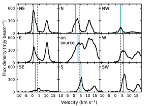
Figure 1: Spectra of the H₂CS 10_0,10 – 9_0,9 line at nine positions toward IRAS 16293A illustrating the variation in line blending across the source. The central panel shows the spectrum in the central pixel (continuum peak), the other spectra are taken at a beam offset (0.5$\arcsec$) in the different directions as denoted in the top left corner of each panel. The vertical dotted line marks the system velocity of 3.8 km s^-1, and the vertical blue solid line indicates the peak velocity from the CH₃OH line used to isolate the target lines (in this case H₂CS 10_0,10 – 9_0,9).

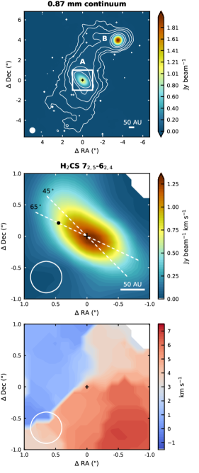
Figure 2: Continuum image of IRAS 16293 at 0.87 mm (top panel) with contour levels at 0.5%, 1%, 2%, 5% and 10% of the peak flux. The white box marks the region around the A source for which the velocity-corrected integrated emission (VINE) map of the H₂CS 7_2,5 – 6_2,4 line at 240.549 GHz ($E_{\rm{u}}$ = 99 K) is shown in the middle panel and the peak velocity at each position in the bottom panel. The continuum peak position of IRAS 16293A is marked with a cross in all panels and the beam is depicted in the lower left corners. The white lines in the middle panel indicate the position angle of the major axis of the disk-like structure found by Oya et al. (2016) (65^∘) and our by-eye best matching position angle of 45^∘. The black circle marks the position where the spectra in Figure 3 are extracted.

2 Observations

The Protostellar Interferometric Line Survey (PILS) is an unbiased spectral survey of the low-mass protobinary IRAS 16293 with the Atacama Large Millimeter/submillimeter Array (ALMA) covering frequencies between 329.147 and 362.896 GHz in Band 7 (project-id: 2013.1.00278.S). Multiple lines from H₂CO, H₂CO isotopologues and H₂CS fall within this spectral range. $\Delta J$ transitions with multiple $K_{\rm{a}}$ transitions available are listed in Table 1. The transition frequencies and other line data were taken from the CDMS database (Müller et al. 2001, 2005). The H₂CO and entries are based on Bocquet et al. (1996), Cornet & Winnewisser (1980), Brünken et al. (2003), and Müller & Lewen (2017), and the H${}_{2}^{13}$CO entries are taken from Müller et al. (2000). Entries of the deuterated isotopologues are based on Dangoisse et al. (1978), Bocquet et al. (1999), and Zakharenko et al. (2015). H₂CS data are provided by Fabricant et al. (1977), Maeda et al. (2008), and Müller et al. (2019).

The data have a spectral resolution of 0.2 km s^-1 (244 kHz), a restoring beam of 0.5$\arcsec$ ($\sim$70 AU), and a sensitivity of 7–10 mJy beam^-1 channel^-1, or $\sim$5 mJy beam^-1 km s^-1 across the entire frequency range. The phase center is located between the two continuum sources at $\alpha$(J2000) = 16^h32^m22$\aas@@fstack{s}$72; $\delta$(J2000) = $-$24$\degr$28$\arcmin$34$\aas@@fstack{\prime\prime}$3. In this work we focus on the A source ($\alpha$(J2000) = 16^h32^m22$\aas@@fstack{s}$873; $\delta$(J2000) =  $-$24$\degr$28$\arcmin$36$\aas@@fstack{\prime\prime}$54). A detailed description of the data reduction and continuum subtraction can be found in Jørgensen et al. (2016).

The PILS program also contains eight selected windows in Band 6 ($\sim$230 GHz) at the same angular resolution as the Band 7 data (0.5$\arcsec$; project-id: 2012.1.00712.S). These data have a spectral resolution of 0.15 km s^-1 (122 kHz) and a sensitivity of $\sim$4 mJy beam^-1 channel^-1, or $\sim$1.5 mJy beam^-1 km s^-1. The data reduction proceeded in the same manner as the Band 7 data (Jørgensen et al. 2016). Several H₂CS $J_{K_{\rm{a}}K_{\rm{c}}}$ = 7_xx – 6_xx transitions are covered by this spectral setup (see Table 1).

IRAS 16293 was also observed at 0.5$\arcsec$ resolution by program 2016.1.01150.S (PI: Taquet). This dataset has a spectral resolution of 0.15 km s^-1 (122 kHz) and a sensitivity of $\sim$1.3 mJy beam^-1 channel^-1, or $\sim$0.5 mJy beam^-1 km s^-1 and covers the H₂CS 7_1,7 – 6_1,6 transition (Table 1). The data reduction is described in Taquet et al. (2018).

3 Results

3.1 Kinematics

The incredible line-richness of IRAS 16293 (on average one line per 3.4 MHz) means that many lines are blended (e.g., Jørgensen et al. 2016). In addition, the large velocity gradient due to the near edge-on rotating structure around the A source ($\sim$6 km s^-1; Pineda et al. 2012; Favre et al. 2014) results in varying line widths and hence varying degrees of blending at different positions (see Fig. 1). Therefore, we make use of the method outlined in Calcutt et al. (2018) to isolate the formaldehyde and thioformaldehyde lines: the peak velocity in each pixel is determined using a bright methanol transition (7_3,5 – 6_4,4 at 337.519 GHz) and this velocity map is then used to identify the target lines listed in Appendix A.

Of the 18 formaldehyde and 15 thioformaldehyde lines, only the H₂CO 5_1,5 – 4_1,4, H${}_{2}^{13}$CO 5_2,4 – 4_2,3, H${}_{2}^{13}$CO 5_4,1 – 4_4,0, D₂CO 6_3,4 – 5_3,3 and H₂CS 7_2,5 – 6_2,4 lines can be fully isolated. Figure 2 shows the Velocity-corrected INtegrated emission (VINE) map for H₂CS 7_2,5 – 6_2,4, that is, the moment zero map but integrated over different velocities in each pixel (Calcutt et al. 2018), as well as a map of the corresponding peak velocities. The emission shows an elongated structure in the northeast-southwest direction along the velocity gradient. The H${}_{2}^{13}$CO 5_1,5 – 4_1,4, H${}_{2}^{13}$CO 5_2,3 – 4_2,2, D₂CO 6_2,5 – 5_2,4 and H₂CS 10_2,9 – 9_2,8 lines are severely blended ($<$ 4 MHz to another line) and excluded from the analysis (see Table 1 for details). All other lines are blended to some degree. In most cases this means that one or both of the line wings in the central pixels ($\sim$0.5$\arcsec$ radius) overlap with the wing of another line.

An overview of the 14 H₂CS lines is shown in Fig. 3 in the form of position-velocity (pv) diagrams along the major axis of the disk-like structure (PA = 65^∘; Oya et al. 2016) and spectra extracted $\sim$0.5$\arcsec$ to the northeast of the source center (see Fig. 2). Similar pv-diagrams for H₂CO, H${}_{2}^{13}$CO and D₂CO are presented in Appendix B. All lines show signs of rotation, that is, low velocities at large angular offsets and high velocities closer to the source center. H₂CO and H₂CS emission extends out to $\gtrsim$2$\arcsec$, while emission from the less abundant isotopologues H${}_{2}^{13}$CO and D₂CO is more compact ($\lesssim$1$\arcsec$), probably due to sensitivity. The emission also becomes more compact for transitions with higher upper level energies, which are expected to trace the warmest inner region. The H₂CO lines show red-shifted absorption for velocities slightly above the systemic velocity of 3.8 km s^-1.

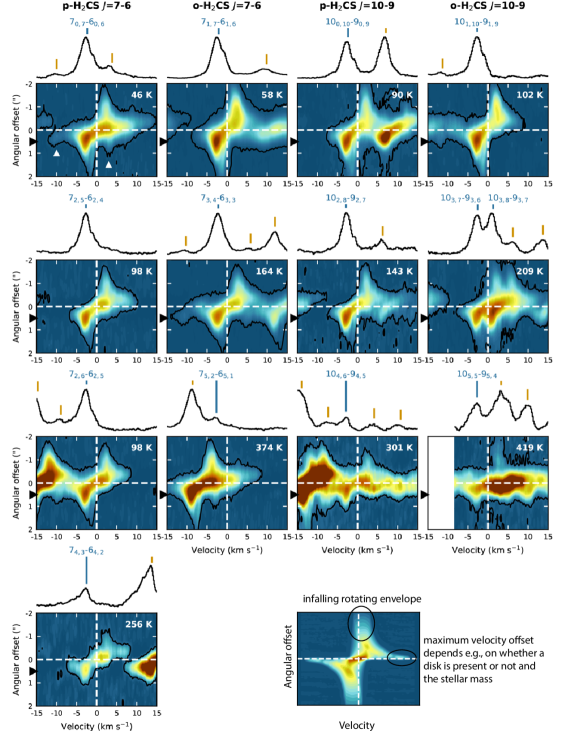
Figure 3: Position-velocity diagrams of the H₂CS lines along the major axis (PA = 65^∘) of the disk-like structure (positive angular offsets denote the northeast direction, i.e. blueshifted emission, negative offsets denote the southwest direction, i.e., redshifted emission). The intensity (color) scale is normalized to the brightest line in each panel. The black contour denotes the 3$\sigma$ contour. The dashed white lines mark the source position and systemic velocity of 3.8 km s^-1 (shifted to 0 km s^-1). The upper level energy is denoted in the top right corner of each panel. The spectra at $\sim$0.5$\arcsec$ northeast of the source (indicated by black triangles left of the vertical axes) are shown on top of the pv-diagram panels. The H₂CS lines are identified by a vertical blue line, other lines by vertical orange lines. The white triangles in the top left panel highlight blending of the 7_0,7 – 6_0,6 line. For reference, the bottom right panel shows the pv-diagram for a thin disk model with keplerian disk and infalling rotating envelope.

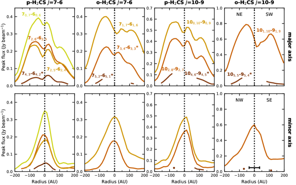
Figure 4: Radial profiles of the H₂CS peak fluxes along the major axis (PA = 45^∘; top panels) and minor axis (PA = 135^∘; bottom panels) of the disk-like structure. In each panel, transitions with higher upper level energy are plotted in darker colors. Fluxes for transitions labeled with an asterisk ($\ast$) have been divided by 2 to account for two transitions with the same upper level energy and Einstein A coefficent at the same frequency (see Table 1). The horizontal bar in the lower right panel marks the beam size. The rms ranges between 2 and 8 mJy beam^-1.

Based on large shifts in velocity from the systemic velocity (up to 14 km s^-1) for the H₂CS 7_0,7 – 6_0,6 line, Oya et al. (2016) suggested that a Keplerian disk may be present inside the centrifugal barrier (at $\sim$50 AU). However, careful analysis of the data shows that a weak line is present on both the blue and red side of this H₂CS line (see Fig. 3, top left panel). The large velocity gradient thus seems the result of line blending and not Keplerian rotation. This conclusion is reinforced by the velocity structure of the other H₂CS lines. The unblended 7_2,5 – 6_2,4 line shows a maximum velocity offset of $\sim$6 km s^-1 on the blue side, and $\sim$10 km s^-1 on the red side. Unblended wings from the other lines show similar offsets. The unblended H₂CS velocity offsets are comparable to the ones for OCS $J=19-18$ (Oya et al. 2016), except for OCS the offset is $\sim$8 km s^-1 on the red side and $\sim$10 km s^-1 on the blue side. Oya et al. (2016) showed that the OCS emission cannot be explained by Keplerian motions, but requires both rotation and infall. A Keplerian component in the inner part of the rotating-infalling disk-like structure can thus not be established with the current observations.

3.2 Peak fluxes

Most lines show some degree of blending, such that generally, in the central pixels ($\sim$0.5$\arcsec$ radius), one or both of the line wings overlap with the wing of another line. As this does not significantly influence the peak flux, we extract the peak flux per pixel in order to make spatial maps of the line ratios and hence temperature structure. Pixels with too much line blending to extract a reliable peak flux are excluded. Since the data cover only one ortho-H₂CO and one para-H₂CO line, the main isotopologue lines cannot be used for a temperature measurement and we exclude H₂CO from further analysis. The D₂CO 6_4,2 – 5_4,1 and 6_4,3 – 5_4,2 lines, as well as the H₂CS 10_3,7 – 9_3,6 and 10_3,8 – 9_3,7 lines, are located within 4 MHz of each other and are too blended to obtain individual peak fluxes (see also Figs. 3 and  12). Maps of the peak fluxes (moment 8 maps) of the remaining H${}_{2}^{13}$CO, D₂CO and H₂CS lines without severe blending are presented in Appendix C and radial profiles for the H₂CS lines are shown in Fig. 4.

All H₂CS lines show an elongated structure with the major axis at $\sim$45^∘ (Figs. 2 and 13). This is slightly different from the 65${}^{\circ}\pm$10^∘ derived by Oya et al. (2016), but radial profiles along a position angle of 45^∘ or 65^∘ are very similar. For all lines, the emission peaks on either side of the continuum peak, as has been seen for most other species toward IRAS 16293A (see e.g., Calcutt et al. 2018; Manigand et al. 2019). This could correspond to the double peaks seen in cm continuum emission (Wootten 1989; Chandler et al. 2005; Pech et al. 2010), although those positions are slightly off (see discussion in Calcutt et al. 2018). Alternatively, they can be due to an edge-on rotating toroidal structure, as, for example, seen in synthetic CO images (Jacobsen et al. 2018). The NE peak is $\sim$60 AU offset from the continuum peak, except for the 7_0,7 – 6_0,6 transition that peaks around $\sim$40 AU (see Fig. 4). The SW peak is around $\sim$25 AU, and is weaker than the NE peak, except for the 7_4,3 – 6_4,2 transition. Most H₂CS lines seem to have a weaker third peak $\sim$120 AU SW off the source center. The H${}_{2}^{13}$CO and D₂CO lines also show an elongated double-peaked structure, albeit more compact and without the third peak seen for H₂CS (Fig. 14). In addition, the northern part is more elongated perpendicular to the major axis than for the H₂CS lines.

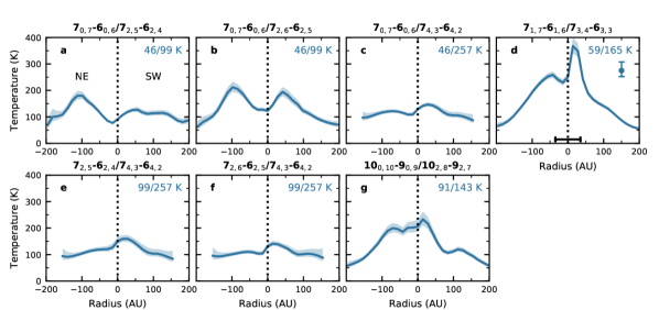
Figure 5: Radial temperature profiles derived from H₂CS line ratios (listed above the panels) along the major axis of the disk-like structure (PA = 45^∘) using the RADEX results. The upper level energies of the transitions are listed in the top right corner of each panel. The shaded area represents the 1$\sigma$ uncertainty based on the noise level of the observations. The vertical bar in the top right panel shows a 3$\sigma$ error bar representative for the inner 100 AU and the horizontal bar marks the beam size.

3.3 Temperature

Only H₂CS lines are used in the temperature analysis, for the reasons outlined below. For H${}_{2}^{13}$CO there are three line ratios that probe temperature (5_0,5 – 4_0,4/5_2,4 – 4_2,3, 5_0,5 – 4_0,4/5_4,1 – 4_4,0 and 5_2,4 – 4_2,3/5_4,1 – 4_4,0), but for the two highest energy lines, the continuum seems to be oversubtracted to varying degrees in different pixels. Reliable peak fluxes can therefore not be obtained for these two lines, leaving only a single suitable H${}_{2}^{13}$CO line and H${}_{2}^{13}$CO is therefore not used to derive the temperature structure. For D₂CO there are six suitable line ratios. However, all these ratios are near unity, suggesting that the emission is optically thick (see Appendix C). Their brightness temperature is $\sim$30 K, much lower than expected for the inner region of an envelope, as also shown for other optically thick lines in the PILS data (e.g., CH₂DOH; Jørgensen et al. 2018), indicating that those lines probe colder foreground material.

The maps of the H₂CS peak fluxes are used to calculate line ratios, and these are converted into temperature maps using a grid of RADEX non-LTE radiative transfer models (van der Tak et al. 2007). The molecular data are obtained from the Leiden Atomic and Molecular Database (LAMDA; Schöier et al. 2005, which contains collisional rate coefficients for H₂CS from Wiesenfeld & Faure 2013). The line ratios as a function of temperature for different H₂ densities and H₂CS column densities are shown in Fig. 15. For densities $\gtrsim$10⁶–10⁷ cm^-3 and column densities $\lesssim$10¹⁵ cm^-2 the line ratios are independent of density and column density, respectively, and thus good tracers of the temperature. For a disk-like structure, densities are expected to be $>10^{7}$ cm^-3, so the exact value adopted for the density does not influence the derived temperatures and we use a value of $10^{10}$ cm^-3. Toward IRAS 16293B, a H₂CS column density of $1.3\times 10^{15}$ cm^-2 was found (Drozdovskaya et al. 2018). As will be discussed later in this section, based on the line ratios, the H₂CS column density toward IRAS 16293A cannot exceed more than a few times $10^{15}$ cm^-2. A column density of $10^{14}$ cm^-2 is adopted in the temperature calculations. All H₂CS lines are optically thin at this column density. At a column of $10^{15}$ cm^-2, the 7_1,7 – 6_1,6 and 10_1,10 – 9_1,9 transitions become optically thick (see Fig. 16), lowering the derived temperature by $\lesssim$10 K (see Fig. 15). In addition to a density and column density, a line width of 2 km s^-1 is adopted to convert the observed line ratios to temperature. Error bars on the line ratios are calculated from the image rms, and converted into error bars on the temperature using the RADEX calculations (see Fig. 15). The error bars therefore depend on the sensitivity of the line ratio to the temperature and the relative uncertainty on the peak flux. Since collisional rate coefficients are not available for all observed transitions, we also performed LTE calculations.

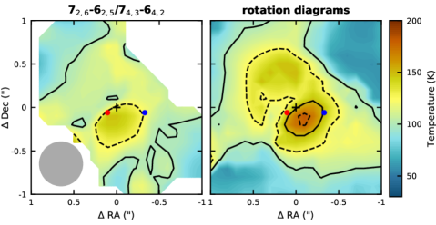
Figure 6: Temperature in a $2^{\prime\prime}\times 2^{\prime\prime}$ (280 $\times$ 280 AU) region around IRAS 16293A derived from the H₂CS 7_2,6 – 6_2,5/7_4,3 – 6_4,2 line ratio (left panel), and from the rotation diagrams in each pixel (right panel). Solid contours indicate temperatures of 100 and 150 K and dashed contours are at 125 and 175 K. The continuum peak position is marked with a black cross. The positions of the unresolved binary components A1 and A2 in 2015 (Hernández-Gómez et al. 2019) are shown with a red and blue circle, resp. The beam is depicted in the lower left corner of the left panel.

Radial temperature profiles along the major axis of the disk-like structure (PA = 45^∘) are presented in Fig. 5 for ratios with collisional rate coefficients and in Fig. 17 for the remaining ratios. Figure 18 shows radial temperature profiles for different position angles. For clarity, we will refer to the panels in Fig. 5 instead of to the quantum numbers of the line ratios in the following discussion. Along the major axis, all line ratios result in temperatures between $\sim$100 and $\sim$175 K out to $\sim$150 AU, with temperatures dropping to $\sim$75 K at $\sim$200 AU. The non-LTE RADEX results give temperatures higher by $\sim$20–50 K than the LTE results (see Fig. 17), suggesting that the lines are not completely thermalized. Panels d and g show temperatures $\gtrsim$150 K in the inner $\sim$100 AU. On the other hand, panels a and b display a decrease in temperature in the inner $\sim$100 AU (down to $\sim$100 K). The other three p-H₂CS ratios (panels c, e and f) show a rather flat temperature profile, with temperatures of $\sim$100–150 K throughout the inner 150 AU. The five line ratios in Fig. 17 cannot be used to constrain the temperature in the inner 100 AU due to severe line blending, but the temperature between $\sim$100–150 AU is $>$100 K. Another constraint can be provided by the ratio between the different $\Delta J$ transitions. The $10-9$ lines are brighter than the $7-6$ lines over the 200 AU radius studied, which means temperatures $\gtrsim$60 K (see Fig. 15).

The central decrease in panels a and b is not likely to be due to the continuum becoming optically thick, because a similar effect would then be expected in panels c, e and f. Instead, it could be due to the fact that the 7_0,7 – 6_0,6 line (which has the lowest upper level energy) peaks closer to the continuum position than the other lines, causing a central increase in the line ratio and hence decrease in the derived temperature. In addition, the temperature derived from these ratios is very sensitive to small changes in the fluxes, because the energy levels involved range from only 46 to 98 K (see Fig. 15). The ratio changes from 1.4 to 1.5 if the temperature drops from 200 K to 150 K, and to 1.8 at 100 K. This means that a variation of $<$10% in one of the peak fluxes can change the derived temperature from 200 K to 150 K, and a 20% variation can change the temperature from 150 K to 100 K. Such variations can occur even though the transitions are present in the same dataset as can be seen from the difference between panels a and b (and Fig. 4, upper left panel). The 7_2,6 – 6_2,5 and 7_2,5 – 6_2,4 transitions have the same upper level energy and Einstein A coefficient, and should thus be equally strong. However, in the SW there is a 100 K difference in the derived temperature using either of the two lines. This variation is slightly larger than the 3$\sigma$ uncertainty based on the rms noise, and may be due to blending with a weak line.

The 7_4,3 – 6_4,2 has a relatively high upper level energy (257 K) and therefore temperatures derived using this transition are less sensitive to flux changes. For example, as the temperature increases from 100 K to 200 K, the 7_0,7 – 6_0,6/7_4,3 – 6_4,2 ratio decreases from 11 to 4.1, and the 7_2,6 – 6_2,5/7_4,3 – 6_4,2 ratio decreases from 6.1 to 2.9. A temperature map for the $2^{\prime\prime}\times 2^{\prime\prime}$ region around IRAS 16293A derived from the 7_2,6 – 6_2,5/7_4,3 – 6_4,2 ratio (panel f) is presented in Fig. 6. The positions of the unresolved binary components of the A source, A1 and A2, are indicated as well. A1 and A2 have been observed to move relative to each other (e.g., Loinard 2002) with a global southwest movement. Since the observations used here are taken between 2014 and 2016, we plot the positions A1 and A2 had in 2015 (Hernández-Gómez et al. 2019). Fig. 6 shows that the radial temperature profiles are not strongly affected by the chosen position angle or the binary components.

The higher temperatures in panels d and g are likely due to optical depth effects. As can be seen from Fig. 16, the 7_1,7 – 6_1,6 and 10_0,10 – 9_0,9 transitions are among the first transitions to become optically thick. If these transitions are optically thick while the higher energy transitions remain optically thin, the flux of the lower energy transition is relatively too low and hence the derived temperature is too high. In turn, an estimate of the H₂CS column density can be made based on these results; for the 7_0,7 – 6_0,6 transition to remain optically thin, the column density of para H₂CS cannot exceed more than a few times 10¹⁵ cm^-2.

To assess whether one of the H₂CS lines is affected by blending with a weak line at a similar frequency and therefore has its peak flux overestimated, rotation diagrams are made for every pixel in a $2^{\prime\prime}\times 2^{\prime\prime}$ region surrounding the continuum position. Representative diagrams at $0.5^{\prime\prime}$ and $1.0^{\prime\prime}$ offsets are presented in Fig. 7. An ortho-to-para ratio of 2 is assumed, but varying this between 1 and 3 changes the derived temperature by $\lesssim$30 K. At offsets $\gtrsim$0.8^′′ all transitions follow a straight line and similar temperatures are found when using all transitions, only ortho transitions or only para transitions in the fit. At smaller angular offsets the scatter becomes larger, but no transition is found to strongly deviate from the general trend. For the lower energy transitions ($E_{\rm{up}}<$ 200 K) this scatter is at least partly because some of the transitions become optically thick.

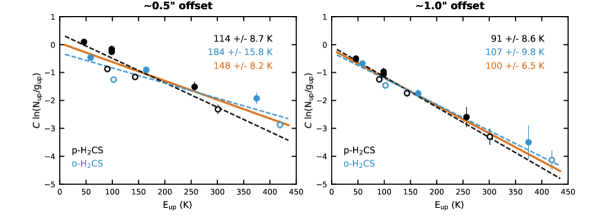
Figure 7: Rotation diagrams for the H₂CS peak fluxes along the major axis (PA = 45^∘) of the disk like structure at 0.5^′′ (left panel) and 1.0^′′ (right panel) from the source center. Para transitions are shown in black and ortho transitions in blue. An ortho-to-para ratio of 2 is assumed. $J=7-6$ transitions are displayed by filled symbols and $J=10-9$ transitions by open symbols. The error bars include a 10% uncertainty. The best fit to all transitions is presented by the solid orange line, whereas the dashed lines show fits to only the ortho (blue) and only the para transitions (black). The corresponding rotation temperatures are listed in the top right corners.

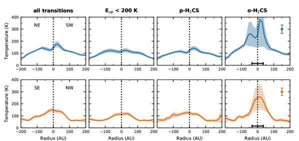
Figure 8: Radial temperature profiles derived from the rotation diagrams including all transitions (first column), only transitions with $E_{\rm{up}}<$ 200 K (second column), only para transitions (third column) or only ortho transitions (fourth column). The top row shows radial profiles along the major axis of the disk-like structure (PA = 45^∘) and the bottom row shows profiles along the minor axis. The shaded area represents the 1$\sigma$ uncertainty. The vertical bar in the right panels shows a typical 3$\sigma$ error for the inner 100 AU and the horizontal bar marks the beam size.

Radial profiles based on the temperatures derived from the rotation diagrams are shown in Fig. 8. These profiles are constructed from fitting either all transitions, only transitions with $E_{\mathrm{up}}<200$ K, only para transitions or only ortho transitions. The first three cases result in temperatures of $\sim$60 K at 200 AU rising up to $\sim$150 at source center. Using only the ortho transitions results in temperatures $>200$ K in the inner 100 AU, likely because the lower energy transitions become optically thick. The central decrease in temperature seen for the 7_0,7 – 6_0,6/7_2,5 – 6_2,4 and 7_0,7 – 6_0,6/7_2,6 – 6_2,5 ratios (panels a and b in Fig. 5) is not seen in these profiles, and may be due to the 7_0,7 – 6_0,6 transition peaking closer in and these ratios being not sensitive to temperature, as discussed above.

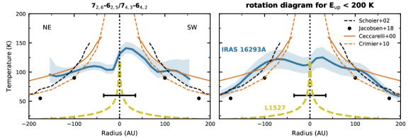
Figure 9: Radial temperature profiles for IRAS 16293A derived in this work from H₂CS transitions (blue lines) compared to dust (black lines and circles) and gas (orange lines) temperature profiles from the literature. The H₂CS temperature profile in the left panel is derived from the 7_2,6 – 6_2,5/7_4,3 – 6_4,2 line ratio and the profile in the right panel is based on fits to the peak flux rotation diagrams including only transitions with $E_{\rm{up}}<$ 200 K. The blue shaded area represents the 1$\sigma$ uncertainty. The dashed black line shows the IRAS 16293 dust temperature assuming an envelope around around a central source of 27 $L_{\odot}$ (Schöier et al. 2002), and the black dots represents dust temperature contours for IRAS 16293A from detailed modeling including both protostars and the bridge structure (Jacobsen et al. 2018). The gas temperatures are based on H₂O observations with the ISO satellite using a model that computes the gas temperature through an envelope by solving a chemical network and equating the heating and cooling rates (Ceccarelli et al. 1996). The solid orange line shows the initial results assuming a single 27 $L_{\odot}$ protostar at 160 pc (Ceccarelli et al. 2000), the dashed orange line presents the revised results for a 22 $L_{\odot}$ protostar at 120 pc (Crimier et al. 2010). The dashed yellow line shows the midplane gas temperature for the Class 0/I disk L1527 based on optically thick ¹³CO and C¹⁸O emission (van ’t Hoff et al. 2018). The horizontal bar marks the beam size of the H₂CS observations.

4 Discussion

Based on line ratios of several $J=7-6$ and $J=10-9$ H₂CS transitions, the temperature in the inner $\sim$ 150 AU of IRAS 16293A is $\sim$100–175 K, and drops to $\sim$75 K at $\sim$200 AU. In Fig. 9, the H₂CS temperature profiles are compared to temperature profiles obtained from continuum radiative transfer modeling and from spatially unresolved H₂O observations with the ISO satellite (Ceccarelli et al. 2000; Schöier et al. 2002; Crimier et al. 2010). These latter profiles were derived assuming a spherically symmetric collapsing envelope structure around a single protostar. Recently, Jacobsen et al. (2018) performed detailed 3D radiative transfer modeling including two protostars. All previously derived temperatures show a very similar structure with a radial power law dependence of approximately $T\propto r^{-0.7}$ in the inner few hundred AU and a temperature of 100 K around $\sim$100 AU. The H₂CS temperature is consistent with the envelope temperature profiles down to radii of $\sim$100 AU, but lacks the temperature rise at smaller radii.

Such a flattening of the temperature could be the result of efficient cooling by water molecules that are released into the gas phase at $\sim$100 K. However, water can also heat the gas through absorption of NIR photons from warm dust. Ceccarelli et al. (1996) studied the gas and dust temperature profile of an infalling envelope with a model that includes dynamics, chemistry, heating and cooling, and concluded that the gas and dust temperatures are generally well-coupled. For different model parameters (e.g., luminosity, mass accretion rate, stellar mass), the difference between the gas and dust temperature ranges from $\sim$10 K to more than a 100 K, but applying this model to IRAS 16293 (assuming a collapsing envelope around a single central source of 27 $L_{\odot}$) results in differences of only a few Kelvin between the gas and dust (Ceccarelli et al. 2000; Crimier et al. 2010). However, this model does not include a disk or disk-like structure. The presence of a disk may result in lower temperatures than in the case of only an envelope, as for example shown by the models from Whitney et al. (2003), observations toward VLA 1623 (Murillo et al. 2015) and analysis of H${}_{2}^{18}$O observations toward four protostars in Perseus (Persson et al. 2016).

A chemical depletion of H₂CS in the inner region is not likely to cause a flat instead of increasing temperature profile, because the line ratios are independent of abundance. The dust opacity could play a role in veiling the hottest inner region, but no absorption, as expected for colder gas in front of warmer dust, is observed. However, the situation is likely complicated with the dust and strongest lines being only marginally optically thick on scales of the beam, but much thicker on smaller unresolved scales. This may lead to quenching of the higher excitation lines while the emission from the lower excitation lines is only slightly reduced, and therefore result in a lower derived excitation temperature. On the other hand, this effect may be mitigated by the fact that multiple lines of sight are integrated in the beam. Detailed radiative transfer modeling is thus required to properly constrain the influence of the dust.

Figure 9 also shows the gas temperature profile for the embedded Class 0/I disk L1527 based on optically thick ¹³CO and C¹⁸O observations (van ’t Hoff et al. 2018), illustrating that the temperature in the disk is $\sim$75 K lower than in the IRAS 16293A disk-like structure. This is consistent with the higher accretion rate and higher luminosity of IRAS 16293A ($\sim 4\times 10^{-6}-5\times 10^{-5}M_{\odot}$ yr^-1 and 18 $L_{\odot}$; Schöier et al. 2002; Jacobsen et al. 2018) compared to L1527 ($3\times 10^{-7}M_{\odot}$ yr^-1 and 1.9-2.6 $L_{\odot}$; Kristensen et al. 2012; Tobin et al. 2012, 2013). As the accretion rate drops in the late stages of the evolution of embedded protostellars, this suggests that the temperature of the disk or disk-like structure drops accordingly.

Oya et al. (2016) also used the 7_0,7 – 6_0,6/7_2,5 – 6_2,4 and 7_0,7 – 6_0,6/7_4,3 – 6_4,2 ratios (Fig. 5, panels a and c) to measure the gas temperature in the envelope, disk and envelope-disk interface (centrifugal barrier). Using the flux within a 0.5^′′ region at 0^′′, 0.5^′′ (70 AU) and 1.0^′′ (140 AU) offsets from the continuum peak position along the disk major axis (PA = 65^∘) integrated over different velocity ranges at each position, they derive temperatures between 70 and 190 K. In addition, they find the highest temperatures at the 0.5^′′ offset position and attribute these temperature increases to weak accretion shocks at the centrifugal barrier ($\sim$50 AU) or to directly heating of a more extended envelope in front of the centrifugal barrier. Although we find a similar temperature range for the inner $\sim$150 AU, we do not see temperature peaks in the 7_0,7 – 6_0,6/7_4,3 – 6_4,2 (Fig. 5, panel c). Peaks are visible for the 7_0,7 – 6_0,6/7_2,5 – 6_2,4 and 7_0,7 – 6_0,6/7_2,6 – 6_2,5 (Fig. 5, panels a and b), but this is likely due to the 7_0,7 – 6_0,6 transition peaking slightly closer to the protostar than the other transitions in combination with the high sensitivity of these ratios to small changes in flux, as discussed in Sect. 3.3. Moreover, no temperature peaks are found from the 7_2,5 – 6_2,4/7_4,3 – 6_4,2 and 7_2,6 – 6_2,5/7_4,3 – 6_4,2 ratios (Fig. 5, panels e and f) or from the rotational diagrams. Additional, higher resolution observations thus seem necessary to substantiate local temperature enhancements at the centrifugal barrier.

5 Conclusions

We used H₂CS line ratios observed in the ALMA-PILS survey to study the gas temperature in the disk-like structure around the Class 0 protostar IRAS 16293A. Because of the line-richness of this source, almost all H₂CS lines are blended in their line wings. Therefore, peak fluxes extracted per pixel are used in the analysis instead of integrated fluxes. Formaldehyde is not used because the optically thick H₂CO and D₂CO lines also trace colder foreground material, and not enough unblended H${}_{2}^{13}$CO transitions were available. Our conclusions can be summarized as follows:

• Strong evidence for a rotationally supported disk is still lacking: the high velocity wings of the H₂CS 7_0,7 – 6_0,6 transition are the result of blending with nearby weak lines instead of a Keplerian disk.

• The temperature is between $\sim$100–175 K in the inner $\sim$150 AU, and drops to $\sim$75 K at $\sim$200 AU. This profile is consistent with envelope temperature profiles constrained on 1000 AU scales down to scales of $\sim$100 AU ($T\propto r^{-0.7}$ in the region where the dust becomes optically thick). However, the envelope profile breaks down in the inner most region that can now be probed by ALMA, because the observed temperature does not show a steep rise at radii $\lesssim$100 AU.

• The temperature in the disk-like structure around IRAS 16293A is $\sim$75 K higher than in the young Class 0/I disk L1527, on similar scales.

The flattening of the temperature profile at radii $\lesssim$100 AU may be the result of efficient cooling by water that has sublimated from the grains in this region. Alternatively, the presence of a disk could affect the temperature structure, by having a larger fraction of the mass at higher density and lower temperatures. High resolution observations of optically thin lines are required to establish the details of the temperature profile in the inner $\sim$100 AU.

Appendix A Formaldehyde and thioformaldehyde lines

Table 1 provides an overview of the H₂CO, H${}_{2}^{13}$CO, D₂CO and H₂CS lines that have $\Delta J$ transitions with multiple $K_{\rm{a}}$ transitions in the spectral coverage of the ALMA-PILS survey.

Table 1: Line list of formaldehyde and thioformaldehyde lines.

Species	Transition	Spin	Frequency	log($A_{ul}$)	$E_{u}$	Used in	Dataset	Notes
		isomer	(GHz)	(s-1)	(K)	analysis
H2CO	50,5 – 40,4	para	362.736	-2.863	52	-	2013.1.00278.S
	51,5 – 41,4	ortho	351.769	-2.920	62	-	2013.1.00278.S
H${}_{2}^{13}$CO	50,5 – 40,4	para	353.812	-2.895	51	-	2013.1.00278.S
	51,5 – 41,4	ortho	343.326	-2.952	61	-	2013.1.00278.S	Blended with H2CS 102,9 – 92,8
	52,3 – 42,2	para	356.176	-2.962	99	-	2013.1.00278.S	CH2DOH at 356.176 GHz
	52,4 – 42,3	para	354.899	-2.966	98	-	2013.1.00278.S
	53,2 – 43,1	ortho	355.203	-3.083	158	-	2013.1.00278.S
	53,3 – 43,2	ortho	355.191	-3.083	158	-	2013.1.00278.S
	54,1 – 44,0	para	355.029	-3.334	240	-	2013.1.00278.S	At same frequency as 54,2 – 44,1
	54,2 – 44,1	para	355.029	-3.334	240	-	2013.1.00278.S	At same frequency as 54,1 – 44,0
D2CO	60,6 – 50,5	para	342.522	-2.933	58	-	2013.1.00278.S	CH2DOH at 342.522 GHz
	61,6 – 51,5	ortho	330.674	-2.989	61	-	2013.1.00278.S
	62,4 – 52,3	para	357.871	-2.925	81	-	2013.1.00278.S
	62,5 – 52,4	para	349.631	-2.955	80	-	2013.1.00278.S	CH2DOH at 349.635 GHz
	63,3 – 53,2	ortho	352.244	-3.019	108	-	2013.1.00278.S
	63,4 – 53,3	ortho	351.894	-3.020	108	-	2013.1.00278.S
	64,2 – 54,1	para	351.492	-3.152	145	-	2013.1.00278.S
	64,3 – 54,2	para	351.487	-3.152	145	-	2013.1.00278.S
	65,1 – 55,0	ortho	351.196	-3.413	194	-	2013.1.00278.S	At same frequency as 65,2 – 55,1
	65,2 – 55,1	ortho	351.196	-3.413	194	-	2013.1.00278.S	At same frequency as 65,1 – 55,0
H2CS	70,7 – 60,6	para	240.267	-3.688	46	yes	2012.1.00712.S
	71,7 – 61,6	ortho	236.727	-3.717	59	yes	2016.1.01150.S
	72,5 – 62,4	para	240.549	-3.724	99	yes	2012.1.00712.S
	72,6 – 62,5	para	240.382	-3.725	99	yes	2012.1.00712.S
	73,4 – 63,3	ortho	240.394	-3.776	165	yes	2012.1.00712.S	At same frequency as 73,5 – 63,4
	73,5 – 63,4	ortho	240.393	-3.776	165	-	2012.1.00712.S	At same frequency as 73,4 – 63,3
	74,3 – 64,2	para	240.332	-3.860	257	yes	2012.1.00712.S	At same frequency as 74,4 – 64,3
	74,4 – 64,3	para	240.332	-3.860	257	-	2012.1.00712.S	At same frequency as 74,3 – 64,2
	75,2 – 65,1	ortho	240.262	-3.998	375	yes	2012.1.00712.S	At same frequency as 75,3 – 65,2
	75,3 – 65,2	ortho	240.262	-3.998	375	-	2012.1.00712.S	At same frequency as 75,2 – 65,1
	100,10 – 90,9	para	342.946	-3.216	91	yes	2013.1.00278.S
	101,9 – 91,8	ortho	348.534	-3.199	105	-	2013.1.00278.S	Several lines at similar frequency
	101,10 – 91,9	ortho	338.083	-3.239	102	yes	2013.1.00278.S
	102,8 – 92,7	para	343.813	-3.231	143	yes	2013.1.00278.S
	102,9 – 92,8	para	343.322	-3.232	143	-	2013.1.00278.S	Blended with H${}_{2}^{13}$CO 51,5 – 41,4
	103,7 – 93,6	ortho	343.414	-3.255	209	-	2013.1.00278.S	Blended with H2CS 103,8 – 93,7
	103,8 – 93,7	ortho	343.410	-3.255	209	-	2013.1.00278.S	Blended with H2CS 103,7 – 93,6
	104,6 – 94,5	para	343.310	-3.290	301	yes	2013.1.00278.S	At same frequency as 104,7 – 94,6
	104,7 – 94,6	para	343.310	-3.290	301	-	2013.1.00278.S	At same frequency as 104,6 – 94,5
	105,5 – 95,4	ortho	343.203	-3.340	419	-	2013.1.00278.S	Not detected
	105,6 – 95,5	ortho	343.203	-3.340	419	-	2013.1.00278.S	Not detected

Appendix B Position-velocity diagrams

Position-velocity diagrams for H₂CO, H${}_{2}^{13}$CO and D₂CO are presented in Figs. 10, 11 and 12, respectively.

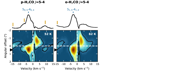
Figure 10: Position-velocity diagrams of the H₂CO lines along the major axis of the disk-like structure (positive angular offsets denote the northeast direction, i.e., blueshifted emission, and negative offsets denote the southwest direction, i.e., redshifted emission). The intensity (color) scale is normalized to the brightest line in each panel. The black contour denotes the 3$\sigma$ contour. The dashed white lines mark the source position and systemic velocity of 3.8 km s^-1 (shifted to 0 km s^-1). The upper level energy is denoted in the top right corner of each panel. The spectra at $\sim$ 0.5$\arcsec$ northeast of the source (indicated by black triangles left of the vertical axes) are shown on top of the pv-diagram panels. The H₂CO lines are identified by a vertical blue line, other lines by vertical orange lines.

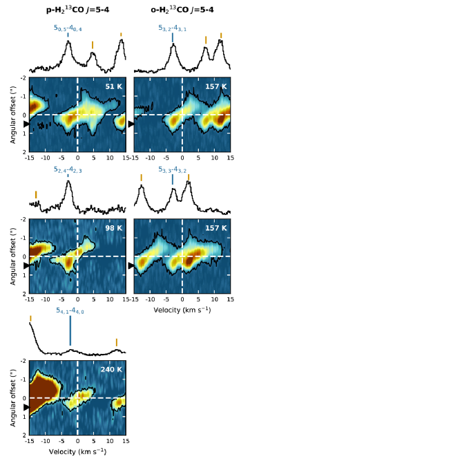
Figure 11: As Fig. 10, but for H${}_{2}^{13}$CO.

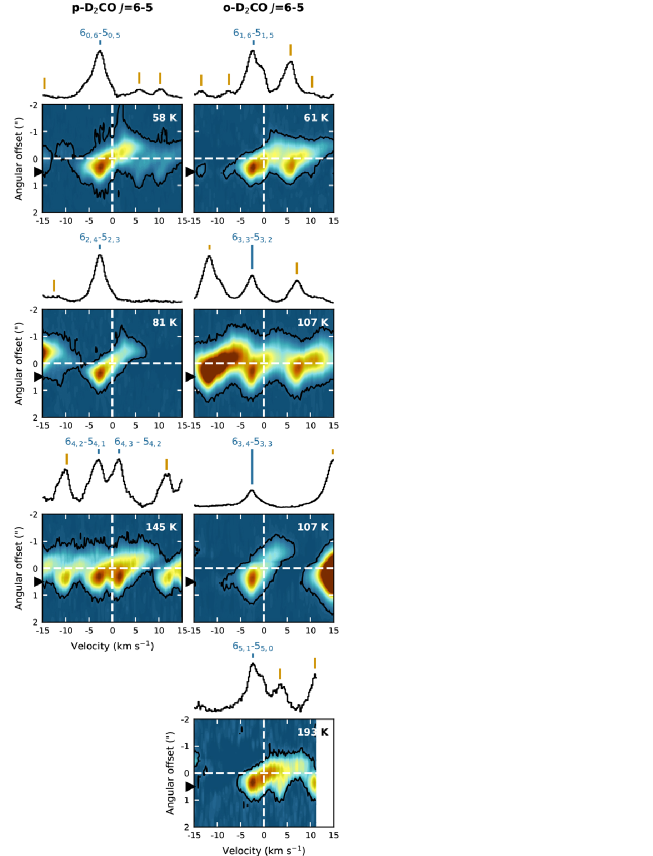
Figure 12: As Fig. 10, but for D₂CO.

Appendix C Peak fluxes

Maps of the peak fluxes (moment 8 maps) are shown in Fig. 13 for H₂CS and in Fig. 14 for H${}_{2}^{13}$CO and D₂CO. Lines that are too blended in the central region to extract reliable peak fluxes are excluded.

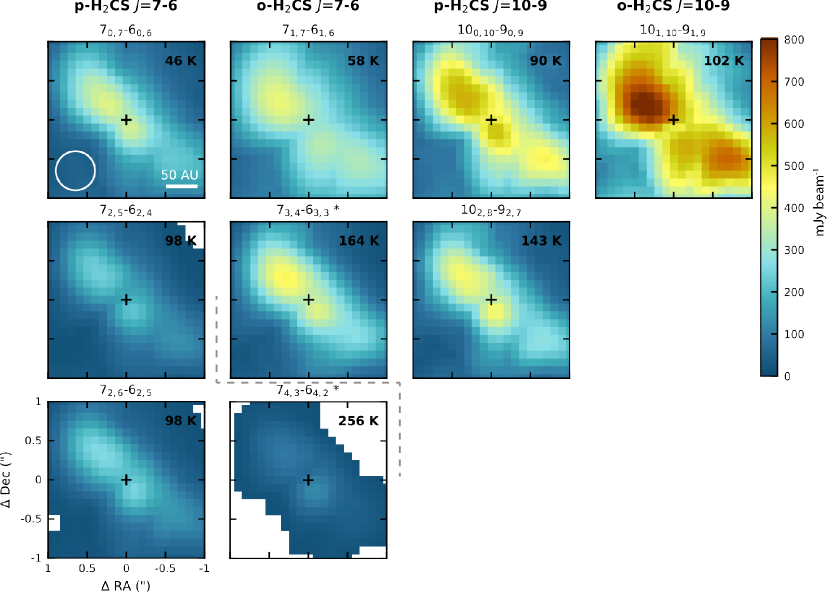
Figure 13: Maps of the peak fluxes (moment 8) of the H₂CS lines. Only lines for which reliable peak fluxes could be extracted in the center, i.e., that are not too blended, are shown. The transitions are denoted above the panels and the corresponding upper level energies are listed in the top right corner of each panel. Asterisks ($\ast$) behind the transition indicate that the flux is coming from two lines with the same $J$ and $K_{\rm{a}}$-level located at the same frequency (see Table 1 for details). All panels are shown at the same intensity (color) scale for comparison. Pixels with no emission $>$3$\sigma$ are masked out. The continuum peak position is marked with a black cross and the beam is depicted in the lower left corner of the top left panel.

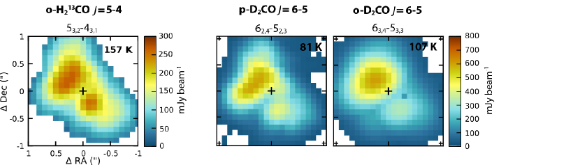
Figure 14: As Fig. 13, but for H${}_{2}^{13}$CO (left panel) and D₂CO (middle and right panel).

Appendix D RADEX results for H₂CS

H₂CS line ratios as function of temperature and density or temperature and column density derived from a grid of non-LTE radiative transfer calculations with RADEX are presented in Fig. 15. Figure 16 shows the column densities at which the different H₂CS lines become optically thick based on the same radiative transfer models.

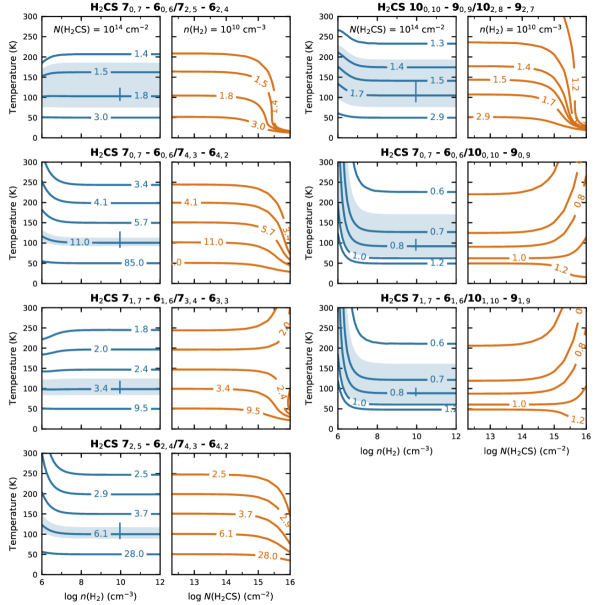
Figure 15: Temperature sensitivity of the H₂CS line ratios as a function of H₂ density (blue lines) and H₂CS column density (orange lines). For the density plots, a H₂CS column density of $10^{14}$ cm^-2 is adopted for both o-H₂CS and p-H₂CS, and a H₂ density of $10^{10}$ cm^-3 is used for the column density plots. The line ratio is listed above the panels and contours are chosen such to mark the ratios at temperatures of 50, 100, 150, 200 and 250 K. The blue shaded area shows the change in derived temperature if the 100 K ratio changes by 20%. The blue vertical line represents the typical 3$\sigma$ error on the temperature based on the observed uncertainty in the line ratio solely due to the rms in the images. The 7_0,7 – 6_0,6/7_2,5 – 6_2,4 ratio is equal to the 7_0,7 – 6_0,6/7_2,6 – 6_2,5 ratio (not shown) and the 7_2,5 – 6_2,4/7_4,3 – 6_4,2 ratio is equal to the 7_2,6 – 6_2,5/7_4,3 – 6_4,2 ratio (not shown).

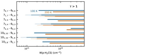
Figure 16: Column densities (expressed in p-H₂CS column density) at which the H₂CS lines are optically thick at 100 K (blue) and 200 K (orange) based on the non-LTE RADEX calculation. For the ortho transitions, solid dark lines assume an ortho-to-para ratio of 1, and the shaded lines assume ortho-to-para ratios of 2 and 3 (lightest shade).

Appendix E Radial temperature profiles

Figure 17 shows radial temperature profiles derived from H₂CS line ratios including transitions for which no collisional rate coefficients are available. These temperatures therefore result from an LTE calculation. Figure 18 presents the radial temperature profiles based on the 7_0,7 – 6_0,6/7_2,5 – 6_2,4 and 7_0,7 – 6_0,6/7_4,3 – 6_4,2 ratios (Fig. 5 panels a and c) for different position angles.

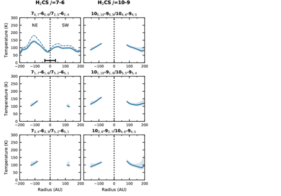
Figure 17: Radial temperature profiles derived from H₂CS line ratios (listed above the panels) for which no collisional rate coefficients are available. The temperature profiles are taken along the major axis of the disk-like structure (PA = 45^∘) and calculated assuming LTE. As a reference, the non-LTE result is shown as well for the 7_0,7 – 6_0,6/7_2,5 – 6_2,4 transition (dashed line in top left panel). The shaded area represents the 1$\sigma$ uncertainty based on statistical errors. The horizontal bar in the top left panel marks the beam size.

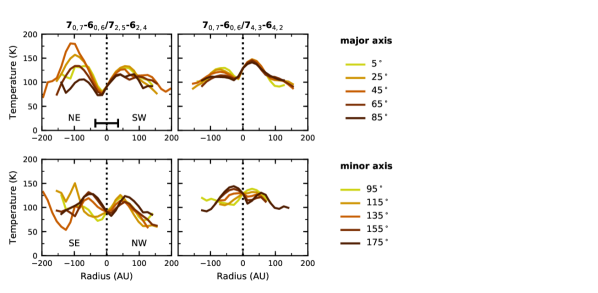
Figure 18: Radial temperature profiles derived from two H₂CS line ratios (listed above the panels) along different position angles (different colors) using the non-LTE RADEX results. A PA of 45^∘ corresponds to the major axis of the disk-like structure as presented in Fig 5. The horizontal bar in the top left panel marks the beam size.