Parallel Data Distribution Management on Shared-Memory Multiprocessors

Abstract.

The problem of identifying intersections between two sets of $d$-dimensional axis-parallel rectangles appears frequently in the context of agent-based simulation studies. For this reason, the High Level Architecture (HLA) specification – a standard framework for interoperability among simulators – includes a Data Distribution Management (DDM) service whose responsibility is to report all intersections between a set of subscription and update regions. The algorithms at the core of the DDM service are CPU-intensive, and could greatly benefit from the large computing power of modern multi-core processors. In this paper we propose two parallel solutions to the DDM problem that can operate effectively on shared-memory multiprocessors. The first solution is based on a data structure (the Interval Tree) that allows concurrent computation of intersections between subscription and update regions. The second solution is based on a novel parallel extension of the Sort Based Matching algorithm, whose sequential version is considered among the most efficient solutions to the DDM problem. Extensive experimental evaluation of the proposed algorithms confirm their effectiveness on taking advantage of multiple execution units in a shared-memory architecture.

1. Introduction

Large agent-based simulations are used in many different areas such human mobility modeling (Klügl and Rindsfüser, 2007), transportation and logistics (Cetin et al., 2002), or complex biological systems (Abraham et al., 2015; Jacob et al., 2004). While there exist recommendations and best practices for designing credible simulation studies (Law, 2009), taming the complexity of large models remains challenging, due to the potentially huge number of virtual entities that need to be orchestrated and the correspondingly large amount of computational resources required to execute the model.

The  High Level Architecture (HLA) has been introduced to partially address the problems above. The HLA is a general architecture for the interoperability of simulators (HLA, 2010b) that allow users to build large models through composition of specialized simulators, called federates according to the HLA terminology. The federates interact using a standard interface provided by a component called  Run-Time Infrastructure (RTI) (HLA, 2010a). The structure and semantics of the data exchanged among the federates are formalized in the  Object Model Template (OMT) specification (HLA, 2010c).

Federates can notify events to other federates, for example to signal a local status update that might impact other simulators. Since notifications might produce a significant overhead in terms of network traffic and processor usage at the receiving end, the RTI provides a  Data Distribution Management (DDM) service whose purpose is to allow federates to specify which notifications they are interested in. This is achieved through a spatial public-subscribe system, where events are associated with an axis-parallel, rectangular region in $d$-dimensional space, and federates can signal the RTI to only receive notifications that overlap one or more subscription regions of interest.

More specifically, HLA allows the simulation model to define a set of dimensions, each dimension being a range of integer values from $0$ to a user-defined upper bound. Dimensions may be used as Cartesian coordinates for mapping the position of agents in 2-D or 3-D space, although the HLA specification does not mandate this. A range is a half-open interval $[\textit{lower bound},\textit{upper bound})$ of values on one dimension. A region specification is a set of ranges, and can be used by federates to denote the “area of influence” of status update notifications. Federates can signal the RTI the regions from which update notifications are to be received (subscription regions). Each update notification is associated with a update region: the DDM service identifies the set of overlapping subscription regions, so that the update message are sent only to federates owning the relevant subscription.

Figure 1. (Top) Road traffic simulation example. (Bottom) A possible mapping of simulated entities (vehicles and traffic lights) to federates.

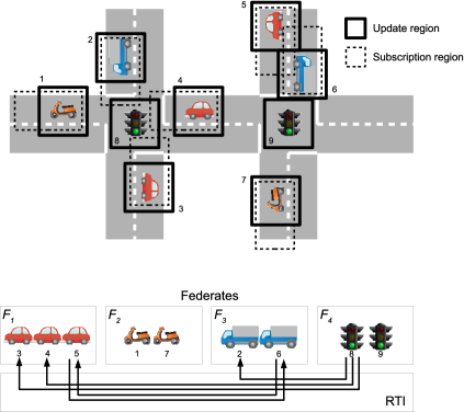
As an example, let us consider the simple road traffic simulation model shown in Figure 1 consisting of vehicles managing intersections. Vehicles need to react both to changes of the color of traffic lights and also to other vehicles in front of them. This can be achieved using suitably defined update and subscription regions. Specifically, each vehicle is enclosed within an update region (thick box) and a subscription region (dashed box), while each traffic light is enclosed within an update region only. A traffic light is a pure generator of update notifications, while vehicles are both producers and consumers of events. Each vehicle generates notifications to signal a change in its position, and consumes events generated by nearby vehicles and traffic lights. We assume that a vehicle can safely ignore what happens behind it; therefore, subscription regions are skewed towards the direction of motion.

If the scenario above is realized through an HLA-compliant simulator, entities need to be assigned to federates. We suppose that there are four federates, $F_{1}$ to $F_{4}$. $F_{1}$, $F_{2}$ and $F_{3}$ handle cars, scooters and trucks respectively, while $F_{4}$ manages the traffic lights. Each simulated entity registers subscription and update regions with the RTI; the DDM service can then match subscription and update regions, so that update notifications can be sent to interested entities. In our scenario, vehicles $2$, $3$ and $4$ receive notifications from the traffic light $8$; vehicles $5$ and $6$ send notifications to each other, since their subscription and update regions overlap. The communication pattern between federates is shown in the bottom part of Figure 1.

As can be seen, at the core of the DDM service there is an algorithm that solves an instance of the general problem of reporting all pairs of intersecting axis-parallel rectangles in a $d$-dimensional space. In the context of DDM, reporting means that each overlapping subscription-update pair must be reported exactly once, without any implied ordering. This problem is well known in computational geometry, and can be solved either using appropriate algorithms and/or ad-hoc spatial data structures as will be discussed in Section 2. However, it turns out that DDM implementations tend to rely on less efficient but simpler solutions. The reason is that spatial data structures can be quite complicated, and therefore their manipulation may require a significant overhead that might be not evident from their asymptotic complexity.

The increasingly large size of agent-based simulations is posing a challenge to the existing implementations of the DDM service. As the number of regions increases, so does the execution time of the intersection-finding algorithms. A possible solution comes from the computer architectures domain. The current trend in microprocessor design is to put more execution units (cores) in the same processor; the result is that multi-core processors are now ubiquitous, so it makes sense to try to exploit the increased computational power to speed up the DDM service (D’Angelo and Marzolla, 2014). Therefore, an obvious parallelization strategy for the intersection-finding problem is to distribute the rectangles across the processor cores, so that each core can work on a smaller problem.

Figure 2. A shared-memory multiprocessor system.

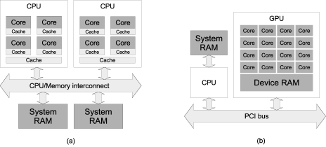
Shared-memory multiprocessors are a family of parallel systems where multiple processors share one or more blocks of Random Access Memory (RAM) through an interconnection network (Figure 2 (a)). A modern multi-core CPU contains multiple independent execution units (cores), that are essentially stand-alone processors. Cache hierarchies within each core, and shared by all cores of the same CPU, are used to mitigate the memory access bottleneck, known as the memory wall (Wulf and McKee, 1995).

General-Purpose GPU computing is another realization of the multi-core paradigm. Graphics Processing Units were originally intended as specialized devices for producing graphical output, but have now evolved into general-purpose parallel co-processors. A high-level overview of a GPU is shown in Figure 2 (b). A GPU includes a large number of cores that share a common memory, called device memory. The device memory is physically separate from the main system RAM, so that programs and data must be transferred from system RAM to device memory before the GPU can start execution. At the end of the computation, results need to be transferred back to system RAM. While a single GPU core is less powerful than a CPU core, a GPU has more cores than a typical CPU, and therefore provides a higher aggregate throughput. However, this comes at a cost: GPU programming is in general more complex than programming a multicore CPU; additionally, CPUs support more memory than GPUs, meaning that CPU-GPU communication might be a bottleneck when processing large datasets. Moreover, GPUs are based on the  Single Instruction Multiple Data (SIMD) paradigm, where a single instruction stream is executed on multiple data items. This paradigm is well suited for applications with regular data access pattern (e.g., linear algebra). Applications with conditional branches or irregular data access patterns may require considerable more effort to be implemented efficiently, but are nevertheless possible: for example, non-trivial but efficient GPU implementations of the Time Warp optimistic synchronization protocol (Liu and Andelfinger, 2017) and of the Bellman-Ford shortest path algorithm (Busato and Bombieri, 2016) have been realized, despite the fact that both fall outside the these application exhibits regular data access patterns. Finally, it must be observed that general-purpose GPUs are currently not as ubiquitous as multicore CPUs, since they are add-on cards that must be purchased separately.

Shared-memory multiprocessors are interesting for several reasons. first, they are ubiquitous since they power virtually everything from smartphones and single-board computers up to high performance computing systems. Moreover, shared-memory architectures are in general simpler to program than distributed-memory architectures, since the latter require explicit message exchanges to share data between processors. Support for shared-memory programming has been added to traditional programming languages such as C, C++ and FORTRAN (Dagum and Menon, 1998), further reducing the effort needed to write parallel applications.

Unfortunately, writing efficient parallel programs is not easy. Many serial algorithms can not be made parallel by means of simple transformations. Instead, new parallel algorithms must be designed from scratch around the features of the underlying execution platform. The lack of abstraction of parallel programming is due to the fact that the user must leverage the strengths (and avoid the weaknesses) of the underlying execution platform in order to get the maximum performance. The result is that, while parallel architectures are ubiquitous – especially shared-memory ones – parallel programs are not, depriving users from a potential performance boost on some classes of applications.

In this paper we present two solutions to the DDM problem that are suitable for shared-memory multiprocessors. The first solution, called  Interval Tree Matching (ITM), is based on the interval tree data structure, that represents subscription or update regions in such a way that intersections can be computed in parallel. The second solution, called Parallel SBM, is a parallel version of  Sort-based Matching (SBM) (Raczy et al., 2005), a state-of-the-art implementation of the DDM service.

This paper is organized as follows. In Section 2, we review the scientific literature related to the DDM service and describe in detail some of the existing DDM algorithms that will be later used in the paper. In Section 3 we describe the interval tree data structure and the ITM parallel matching algorithm. In Section 4, we present the main contribution of this work, i.e., a parallel version of the SBM algorithm. In Section 5 we experimentally evaluate the performance of parallel SBM on two multi-core processors. Finally, the conclusions will be discussed in Section 6.

2. Problem statement and existing solutions

In this paper we address the region matching problem defined as follows:

Region Matching Problem. Given two sets $\mathbf{S}=\{S_{1},\ldots,S_{n}\}$ and $\mathbf{U}=\{U_{1},\ldots,U_{m}\}$ of $d$-dimensional, axis-parallel rectangles (also called $d$-rectangles), enumerate all pairs $(S_{i},U_{j})\subseteq\mathbf{S}\times\mathbf{U}$ such that $S_{i}\cap U_{j}\neq\emptyset$; each pair must be reported exactly once, in no particular order.

Figure 3. An example of the region Matching Problem in $d=2$ dimensions. The list of overlapping (subscription, update) pairs is $\{(S_{1},U_{1}),(S_{2},U_{2}),(S_{3},U_{1}),(S_{3},U_{2})\}$

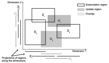
Although the HLA specification only allows integer coordinates, we address the more general case in which the coordinates of the edges of the $d$-rectangles are arbitrary real numbers.

Figure 3 shows an instance of the region matching problem in $d=2$ dimensions with three subscription regions $\mathbf{S}=\{S_{1},S_{2},S_{3}\}$ and two update regions $\mathbf{U}=\{U_{1},U_{2}\}$. In this example there are four overlapping subscription-update pairs $\{(S_{1},U_{1}),\ (S_{2},U_{2}),\ (S_{3},U_{1}),\ (S_{3},U_{2})\}$.

The time complexity of the region matching problem is output-sensitive, since it depends on the size of the output in addition to the size of the input. Therefore, if there are $K$ overlapping regions, any region matching algorithm requires time $\Omega(K)$. Since there can be at most $n\times m$ overlaps, the worst-case complexity of the region matching problem is $\Omega(n\times m)$. In practice, however, the number of intersections is much smaller than $n\times m$.

Algorithm 1 Intersect-1D$(x,y)$

return $x.\emph{low}\leq y.\emph{high}\wedge\ y.\emph{low}\leq x.\emph{high}$

One of the key steps of any matching algorithm is testing whether two $d$-rectangles overlap. The case $d=1$ is very simple, as it reduces to testing whether two half-open intervals $x=[x.\textit{low},x.\textit{high})$, $y=[y.\textit{low},y.\textit{high})$ intersect; this happens if and only if

$$x.\emph{low}<y.\emph{high}\wedge\ y.\emph{low}<x.\emph{high}$$

(see Algorithm 1).

The case $d>1$ can be reduced to the case $d=1$ by observing that two $d$-rectangles overlap if and only if their projections along each dimension overlap. For example, looking again at Figure 3 we see that the projections of $U_{1}$ and $S_{1}$ overlap on both dimensions, so we can conclude that the regions $U_{1}$ and $S_{1}$ intersect. Therefore, any algorithm that solves the region matching problem for two sets of $n$ and $m$ segments in time $O\left(f(n,m)\right)$ can be extended to an $O\left(d\times f(n,m)\right)$ algorithm for the $d$-dimensional case, by executing the 1-D algorithm on each dimension and computing the intersection of the partial results. Since the parameter $d$ is fixed for every problem instance, and much smaller than $n$ or $m$, it can be treated as a constant so we get $O\left(d\times f(n,m)\right)\subset O\left(f(n,m)\right)$. Therefore, solving the general case is, under reasonable circumstances, asymptotically not harder than solving the special case $d=1$.

In the rest of this section we provide some background on the region matching problem. We report some known lower bounds for specific formulations of this problem; we then review some algorithms and data structures that have been developed in the context of computational geometry research. Finally, we describe in details some relevant solutions developed within the HLA research community: Brute Force Matching (BFM), Grid Based Matching (GBM), and Sort-based Matching (SBM). Since we will frequently refer to these algorithms in this paper, we provide all the necessary details below. A comprehensive review of the $d$-dimensional region matching problem is outside the scope of this work, and has already been carried out by Liu and Theodoropoulos (Liu and Theodoropoulos, 2014) to which the interested reader is referred.

Lower Bounds

Over time, several slightly different formulations of the region matching problem have been considered. The most common formulation is to find all overlapping pairs among a set of $N$ rectangles, without any distinction between subscription and update regions. One of the first efficient solutions for this problem is due to Bentley and Wood (Bentley and Wood, 1980) who proposed an algorithm for the two-dimensional case requiring time $\Theta(N\lg N+K)$, where $K$ is the cardinality of the result. They proved that the result is optimal by showing a lower bound $\Omega(N\lg N+K)$ for this type of problem.

Petty and Morse (Petty and Morse, 2004) studied the computational complexity of the following formulation of the region matching problem: given an initially empty set $R$ of $d$-dimensional regions, apply a sequence of $N$ operations of any of the following types: (i) insert a new region in $R$; (ii) delete an existing region from $R$; (iii) enumerate all regions in $R$ overlapping with a given test region. They showed that a lower bound on the computational complexity of this problem is $\Omega(N\lg N)$ by reduction to binary search, and an upper bound is $O(N^{2})$; the upper bound can be achieved with the Brute Force algorithm that we will describe shortly.

Computational Geometry approaches

The problem of counting or enumerating intersections among $d$-dimensional rectangles is of great importance in computational geometry, and as such received considerable attention. Existing approaches rely on a combination of algorithmic techniques such as sorting, searching and partitioning (Six and Wood, 1980, 1982; Bentley and Wood, 1980; Edelsbrunner, 1983), and data structures used to speed up various types of spatial queries (containment, overlap, counting, filtering).

The aforementioned algorithm by Bentley and Wood (Bentley and Wood, 1980) can report all intersections within a set of $N$ rectangles in time $\Theta(N\lg N+K)$. The algorithm is quite complex and operates in two phases: the first phase takes care of rectangles whose sides intersect using the algorithm described in (Bentley and Ottmann, 1979); the second phase takes care of those rectangles which are contained into another one, using a data structure called segment tree. While the algorithm is optimal, it cannot be generalized for the case $d>2$ and its implementation is nontrivial.

A simpler algorithm for the case $d=2$ has been discovered by Six and Wood (Six and Wood, 1980). The algorithm works by sorting the endpoints of the rectangles along one of the dimensions, and then scanning the endpoints updating an auxiliary data structure called interval tree (which, despite the similar name, is not related to the interval tree that will be described in Section 3). The algorithm by Six and Wood runs in time $\Theta(N\lg N+K)$, but is much easier to implement than Bentley and Wood’s. A generalization for the case $d>2$ has been described in (Six and Wood, 1982) and requires time $O\left(2^{d-1}n\lg^{d-1}n+K\right)$ and space $O\left(2^{d-1}n\lg^{d-1}n\right)$.

Edelsbrunner (Edelsbrunner, 1983) proposed an improved algorithm based on a rectangle tree data structure that can report all intersections among a set of $N$ $d$-rectangles in time $O\left(N\lg^{2d-3}N+K\right)$ and space $O\left(N\lg^{d-2}N\right)$, thus improving the previous results.

Spatial data structures for the rectangle intersection problem include the $k$-$d$ tree (Rosenberg, 1985), the quad-tree (Finkel and Bentley, 1974), the R-tree (Guttman, 1984) and the BSP tree (Naylor et al., 1990). These data structures use various types of hierarchical spatial decomposition techniques to store volumetric objects. Spatial data structures are widely used in the context of geographical information systems, since they allow efficient execution of range queries, e.g., reporting all objects inside a user-specified range. However, some of these data structures have been adapted to solve the DDM problem. For example, Eroglu et al. (Eroglu et al., 2008) use a quad-tree to improve the grid-based matching algorithm used in HLA implementations.

In (Junghyun Ahn and Kim, 2012) the authors propose a binary partition-based matching algorithm whose aim is to reduce the number of overlap tests that need to be performed between subscription and update regions. Experimental evaluation shows that the algorithm works well in some settings, but suffers from a worst case cost of $O(N^{2}\lg N)$ where $N$ is the total number of subscription and update regions.

Geometric algorithms and data structures have the drawback of being quite complex to implement and, in many real-world situations, slower than less efficient but simpler solutions. For example, Petty and Mukherjee (Petty and Mukherjee, 1997) showed that a simple grid-based matching algorithm performs faster than the $d$-dimensional quad-tree variant from (Van Hook et al., 1996). Similarly, Devai and Neumann (Devai and Neumann, 2010) propose a rectangle-intersection algorithm that is implemented using only arrays and that can enumerate all $K$ intersections among $N$ rectangles in time $O(N\lg N+K)$ time and $O(N)$ space.

Brute-Force Matching

Algorithm 2 BruteForce-1D$(\mathbf{S},\mathbf{U})$

1:for all subscription intervals $s\in\mathbf{S}$ do

2:     for all update intervals $u\in\mathbf{U}$ do

3:         if Intersect-1D($s,u$) then Report($s,u$)               

The simplest solution to the segment intersection problem is the BFM approach, also called Region-Based matching (Algorithm 2). The BFM algorithm, as the name suggests, checks all $n\times m$ subscription-update pairs $(s,u)$ and reports every intersection by calling a model-specific function Report($s$, $u$) whose details are not shown.

The BFM algorithm requires time $\Theta(nm)$; therefore, it is optimal only in the worst case, but very inefficient in general. However, BFM exhibits an embarrassingly parallel structure since the loop iterations (lines 1–3) are independent. Therefore, on a shared-memory architecture with $P$ processors it is possible to distribute the iterations across the processors; each processor will then operate on a subset of $nm/P$ intervals without the need to interact with other processors. The parallel version of BFM requires time $\Theta(nm/P)$.

Grid-Based Matching

Figure 4. Grid-based matching in $d=2$ dimensions.

Algorithm 3 Grid-1D$(\mathbf{S},\mathbf{U})$

1:$\mathit{ncells}\ \textrm{number of grid cells}$

2:$G\leftarrow\textrm{array}[0..\mathit{ncells}-1]\ \textrm{of empty lists}$

3:$\mathit{lb}\leftarrow\textrm{minimum of the lower bounds of all intervals in $\mathbf{S}\cup\mathbf{U}$}$

4:$\mathit{ub}\leftarrow\textrm{maximum of the upper bounds of all intervals in $\mathbf{S}\cup\mathbf{U}$}$

5:$\mathit{width}\leftarrow(\mathit{ub}-\mathit{lb})/\mathit{ncells}$

6:for all update regions $u\in\mathbf{U}$ do$\triangleright$ Build the grid

7:     $i\leftarrow\lfloor(u.\mathit{lower}-\mathit{lb})/\mathit{width}\rfloor$

8:     while $(i<\mathit{ncells})\ \wedge\ (i\times\mathit{width}<u.\mathit{upper})$ do

9:         Add $u$ to the list $G[i]$

10:         $i\leftarrow i+1$      

11:$\mathit{res}\leftarrow\emptyset$

12:for all subscription regions $s\in\mathbf{S}$ do$\triangleright$ Find intersections

13:     $i\leftarrow\lfloor(s.\mathit{lower}-\mathit{lb})/\mathit{width}\rfloor$

14:     while $(i<\mathit{ncells})\ \wedge\ (i\times\mathit{width}<s.\mathit{upper})$ do

15:         for all update regions $u\in G[i]$ do

16:              if $\textsc{Intersect-1D}(s,u)\ \wedge\ (s,u)\notin\mathit{res}$ then

17:                  $\mathit{res}\leftarrow\mathit{res}\cup(s,u)$

18:                  Report($s,u$)                        

19:         $i\leftarrow i+1$      

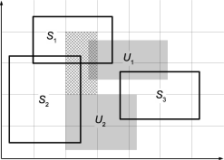
The GBM algorithm (Van Hook et al., 1996; Boukerche et al., 2005) improves over BFM by trying to reduce the number of pairs that are checked for overlap. GBM works by partitioning the domain into a regular mesh of $d$-dimensional cells. Each subscription or update region is mapped to the grid cells it overlaps with. Events generated by an update region $U_{j}$ are sent to all subscription regions that share at least one cell with $U_{j}$. However, this could generate spurious notifications: for example, the subscription region $S_{2}$ in Figure 4 shares the hatched grid cells with $U_{1}$, but does not overlap with $U_{1}$. Spurious notifications can be eliminated by testing for overlap all subscription and update regions sharing the same grid cell. Essentially, this is equivalent to applying the brute-force (or any other region matching) algorithm to the regions sharing the same grid cell (Tan et al., 2000b).

Algorithm 3 shows an implementation of GBM for the case $d=1$. The algorithm consists of two phases. During the first phase (lines 6–10) the algorithm builds an array $G$ of lists, where $G[i]$ contains the update regions that overlap with the $i$-th grid cell. The grid cells are determined by first computing the bounding interval $[\mathit{lb},\mathit{ub})$ of all regions in $\mathbf{S}$ and $\mathbf{U}$. Then, the bounding interval is evenly split into $\mathit{ncells}$ segments of width $(\mathit{ub}-\mathit{lb})/\mathit{ncells}$ so that the $i$-th grid cell corresponds to the interval $[\mathit{lb}+i\times\mathit{width},\mathit{lb}+(i+1)\times\mathit{width})$. The parameter $\mathit{ncells}$ must be provided by the user.

During the second phase (lines 12–19), the algorithm scans the list of subscription regions. Each subscription region is compared with the update regions on the lists of the cells it overlaps with (line 16). Since subscription and update regions may span more than one grid cell, the algorithm keeps a set $\mathit{res}$ of all intersections found so far in order to avoid reporting the same intersection more than once.

If the regions are evenly distributed, each grid cell will contain $n/\mathit{ncells}$ subscription and $m/\mathit{ncells}$ update intervals on average. Therefore, function Intersect-1D will be called $O(\mathit{ncells}\times n\times m/\mathit{ncells}^{2})=O(n\times m/\mathit{ncells})$ times on average. Initialization of the array $G$ requires time $O(\mathit{ncells})$. The upper and lower bounds $\mathit{lb}$ and $\mathit{ub}$ can be computed in time $O(n+m)$. If the set $\mathit{res}$ is implemented using bit vectors, insertions and membership tests can be done in constant time. We can therefore conclude that the average running time of Algorithm 3 is $O(\mathit{ncells}+n\times m/\mathit{ncells})$.

The average-case analysis above only holds if subscription and update regions are uniformly distributed over the grid, which might or might not be the case depending on the simulation model. For example, in the presence of a localized cluster of interacting agents, it might happen that the grid cells around the cluster have a significantly larger number of intervals than other cells. Additionally, the number of cells $\mathit{ncells}$ is a critical parameter. Tan et al. (Tan et al., 2000a) showed that the optimal cell size depends on the simulation model and on the execution environment, and is therefore difficult to predict a priori.

Observe that the iterations of the loop on lines 12–19 are independent and can therefore be executed in parallel. If we do the same for the loop on lines 6–10, however, a data race arises since multiple processors might concurrently update the list $G[i]$. This problem can be addressed by ensuring that line 9 is executed atomically, e.g., by enclosing it inside a critical section or employing a suitable data structure for the lists $G[i]$ that supports concurrent appends. We will discuss this in more details in Section 5. Finally, it is worth noticing that some variants of GBM have been proposed to combine the grid-based method with a region-based strategy (Boukerche and Roy, 2002).

Algorithm 4 Sort-Based-Matching-1D$(\mathbf{S},\mathbf{U})$

1:$T\leftarrow\emptyset$

2:for all regions $x\in\mathbf{S}\cup\mathbf{U}$ do

3:     Insert $x.\textit{lower}$ and $x.\textit{upper}$ in $T$

4:Sort $T$ in non-decreasing order

5:$\texttt{SubSet}\leftarrow\emptyset$, $\texttt{UpdSet}\leftarrow\emptyset$

6:for all endpoints $t\in T$ in non-decreasing order do

7:     if $t$ belongs to subscription region $s$ then

8:         if $t$ is the lower bound of $s$ then

9:              $\texttt{SubSet}\leftarrow\texttt{SubSet}\cup\{s\}$

10:         else

11:              $\texttt{SubSet}\leftarrow\texttt{SubSet}\setminus\{s\}$

12:              for all $u\in\texttt{UpdSet}$ do Report($s,u$)                        

13:     else$\triangleright$ $t$ belongs to update region $u$

14:         if $t$ is the lower bound of $u$ then

15:              $\texttt{UpdSet}\leftarrow\texttt{UpdSet}\cup\{u\}$

16:         else

17:              $\texttt{UpdSet}\leftarrow\texttt{UpdSet}\setminus\{u\}$

18:              for all $s\in\texttt{SubSet}$ do Report($s,u$)                             

Figure 5. Value assigned by the SBM algorithm to the SubSet variable as the endpoints are swept from left to right.

Sort-Based Matching

Sort-based Matching (Jun et al., 2002; Raczy et al., 2005) is an efficient solution to the region matching problem in $d=1$ dimensions. SBM scans the sorted list of endpoints of the subscription and update intervals, keeping track of which regions are active at any point; a region is active if the left endpoint has been scanned, but the right endpoint has not. When the right endpoint of a subscription (resp., update) region $x$ is encountered, all currently active update (resp., subscription) regions are known to overlap with $x$.

The SBM algorithm is illustrated in Algorithm 4. Given $n$ subscription intervals $\mathbf{S}$ and $m$ update intervals $\mathbf{U}$, SBM considers each of the $2\times(n+m)$ endpoints in non-decreasing order; two sets SubSet and UpdSet are used to keep track of the active subscription and update regions, respectively, at every point $t$. When the upper bound of an interval $x$ is encountered, it is removed from the corresponding set of active regions, and the intersections between $x$ and every active region of the opposite kind are reported. Observe that Algorithm 4 never calls the function Intersect-1D to check whether two regions overlap. Figure 5 illustrates how the SubSet variable is updated while SBM sweeps through a set of subscription intervals (update intervals are handled in the same way).

Let $N=n+m$ be the total number of intervals; then, the number of endpoints is $2N$. The SBM algorithm uses simple data structures and requires $O\left(N\lg N\right)$ time to sort the vector of endpoints, plus $O(N)$ time to scan the sorted vector. During the scan phase, $O(K)$ time is spent to report all $K$ intersections. The overall computational cost of SBM is therefore $O\left(N\lg N+K\right)$.

Li et al. (Li et al., 2018) improved the SBM algorithm by reducing the size of the vectors to be sorted and employing the binary search algorithm on the (smaller) sorted vectors of endpoints. The execution time is still dominated by the $O\left(N\lg N\right)$ time required to sort the smaller vectors of endpoints, but the improved algorithm is faster in practice than SBM due to lower constants hidden in the asymptotic notation.

Pan et al. (Pan et al., 2011) extended SBM to deal with a dynamic setting where regions are allowed to change their position or size without the need to execute the SBM algorithm from scratch after each update.

So far, no parallel version of SBM exists. SBM cannot be easily parallelized due to the presence of a sequential scan phase that is intrinsically serial. This problem will be addressed in Section 4, where a parallel version of SBM will be described.

Parallel algorithms for the region matching problem

So far, only a few parallel algorithms for the region matching problem have been proposed. Liu and Theodoropoulos (Liu and Theodoropoulos, 2009, 2013) propose a parallel region matching algorithm that partitions the routing space into blocks, and assigns partitions to processors using a master-worker paradigm. Each processor then computes the intersections among the regions that overlap the received partitions. In essence, this solution resembles a parallel version of the GBM algorithm.

In (Rao et al., 2013) the performance of parallel versions of BFM and grid-based matching (fixed, dynamic and hierarchical) are compared. In this case, the preliminary results presented show that the parallel BFM has a limited scalability and that, in this specific case, the hierarchical grid-based matching has the best performance.

In (Liu et al., 2015), a parallel ordered-relation-based matching algorithm is proposed. The algorithm is composed of five phases: projection, sorting, task decomposition, internal matching and external matching. In the experimental evaluation, a MATLAB implementation is compared with the sequential SBM. The results show that, with a high number of regions the proposed algorithm is faster than SBM.

3. Parallel Interval Tree Matching

In this section we describe the parallel ITM algorithm for solving the region matching problem in one dimension. ITM (Marzolla et al., 2013) is based on the interval tree data structure. An interval tree is a balanced search tree that stores a dynamic set of intervals; it supports insertions, deletions, and queries to get the list of segments that intersect a given interval $q$.

Figure 6. Interval Tree representation of a set of intervals

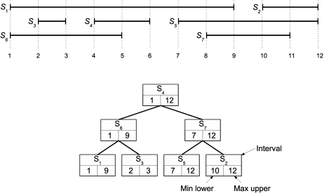
Figure 6 shows a set of intervals and their tree representation. The tree is realized using an augmented AVL tree (Adelson-Velskii and Landis, 1962) as described in (Cormen et al., 2009, Chapter 14.3). Each node $x$ contains three fields: (i) an interval $x.\textit{in}$, represented by its lower and upper bounds; (ii) the minimum lower bound $x.\textit{minlower}$ among all intervals stored at the subtree rooted at $x$; (iii) the maximum upper bound $x.\textit{maxupper}$ among all intervals stored at the subtree rooted at $x$.

Insertions and deletions are handled according to the normal rules for AVL trees, with the additional requirement that any update of the values of maxupper and minlower must be propagated up to the root. During tree operations, nodes are kept sorted according to the lower bounds. Since the height of an AVL tree is $\Theta(\lg n)$, insertions and deletions in the augmented data structure require $O(\lg n)$ time in the worst case. Creating a new tree with $n$ nodes requires total time $O(n\lg n)$ and space $O(n)$.

Algorithm 5 Interval-Tree-Matching-1D$(\mathbf{S},\mathbf{U})$

1:function Interval-Query($\textit{node},q$)

2:     if $\textit{node}=\textit{null}$ $\vee$ $\textit{node}.\textit{maxupper}<q.\textit{lower}$ $\vee$ $\textit{node}.\textit{minlower}>q.\textit{upper}$ then

3:         return      

4:     Interval-Query($\textit{node}.\textit{left},q$)

5:     if Intersect-1D($\textit{node}.\textit{in},q$) then

6:         Report($\textit{node}.\textit{in},q$)      

7:     if $q.\textit{upper}\geq\textit{node}.\textit{in}.\textit{lower}$ then

8:         Interval-Query($\textit{node}.\textit{right},q$)      

9:

10:$T\leftarrow\textrm{create interval tree for $\mathbf{S}$}$

11:for all update regions $u\in\mathbf{U}$ in parallel do

12:     Interval-Query($T.\textit{root},u$)

Algorithm 5 illustrates how parallel ITM works. The first step is to build an interval tree $T$ containing the subscription intervals $\mathbf{S}$ (the details are omitted for the sake of conciseness; Section 5 provides directions to the source code). Function Interval-Query($T.\textit{root},u$) is then used to report all intersections among an update region $u$ and all subscription intervals stored in $T$. The procedure is similar to a conventional binary search tree lookup, using the $x.\textit{minlower}$ and $x.\textit{maxupper}$ fields of every node $x$ to steer the visit away from irrelevant subtrees. Since each node represents one interval, function Interval-Query reports each intersection only once.

Asymptotic execution time

An interval tree can be created in time $O(n\lg n)$ like an ordinary AVL tree. To determine the cost of one invocation of function Interval-Query we first observe that each node can be visited at most once per call, so $O(n)$ is an upper bound on the asymptotic running time of Interval-Query. If region $u$ overlaps with $K_{u}$ subscription intervals, then the execution time of Interval-Query($T.\mathit{root},u$) is also bound by $O(K_{u}\lg n)$; combining the two bounds we get that one call costs $O\left(\min\{n,K_{u}\lg n\}\right)$. Since function Interval-Query is called $m$ times (one for each update region $u$), the total query time is $O\left(\min\{m\times n,K\lg n\}\right)$, $K$ being the number of intersections.

Once the tree is built, its structure is never modified. Therefore, the iterations of the loop on lines 11–12 can be evenly split across $P$ processors on a shared-memory architecture. The parallel query time is then reduced by a factor $P$ and becomes $O\left(\min\{m\times n,K\lg n\}/P\right)$.

Observe that Algorithm 5 allows the roles of $\mathbf{S}$ and $\mathbf{U}$ to be swapped. This can be helpful if the number of update regions $m$ is much lower than the number of subscription regions $m$. If $m\ll n$ it is more convenient to build a tree on $\mathbf{U}$ instead than on $\mathbf{S}$, since the height will be lower. With this optimization we can replace $n$ with $m$ in the asymptotic query time above.

Different implementations of the interval tree are possible. Priority search trees (McCreight, 1985) support insertion and deletion in time $O(\lg n)$, and can report all $K$ intersections with a given query interval in time $O(K+\lg n)$. While the implementation above based on AVL trees is asymptotically less efficient, it has the advantage of being easier to implement since it relies on a familiar data structure. We have chosen AVL trees over other balanced search trees, such as red-black trees (Guibas and Sedgewick, 1978), because AVL trees are more rigidly balanced and therefore allow faster queries. It should be observed that ITM is not tied to any specific interval tree implementation; therefore, any data structure can be used as a drop-in replacement.

Dynamic interval management

An interesting feature of ITM is that it can easily cope with dynamic intervals. The HLA specification allows federates to modify (i.e., move or grow/shrink) subscription and update regions; the ability to do so is indeed essential in almost every agent-based simulation model. A subscription region $s\in\mathbf{S}$ (resp. $u\in\mathbf{U}$) changing its position or size will trigger at most $O(m)$ (resp. $O(n)$) new overlaps, so it makes sense to exploit the data structures already built instead of running the matching phase from scratch each time.

The interval tree data structure can be used to implement a dynamic data distribution management scenario as follows. We can use two interval trees $T_{U}$ and $T_{S}$ holding the set of update and subscription regions, respectively. If an update region $u\in\mathbf{U}$ is modified, we can identify the $K_{u}$ subscriptions overlapping with $u$ in time $O\left(\min\{n,K_{u}\lg n\}\right)$ ($O\left(\min\{n,K_{u}\lg n\}/P\right)$ if $P$ processors are used) by repeatedly calling the function Interval-Query on $T_{U}$. Similarly, if a subscription region $s\in\mathbf{S}$ changes, the $K_{s}$ overlaps with $s$ can be computed in time $O\left(\min\{m,K_{s}\lg m\}\right)$ using $T_{U}$. When a subscription or update region is modified, the appropriate tree must be updated by deleting and re-inserting the node representing the region that changed. These operations require time $O(\lg n)$ for the subscription regions, and $O(\lg n)$ for the update regions.

4. Parallel Sort-based Matching

The parallel ITM algorithm from the previous section relies on a data structure (the interval tree) to efficiently enumerate all intersections among a set of intervals with a given query interval $q$. Once built, the interval tree allows a high degree of parallelism since all update regions can be compared concurrently with the subscription regions stored in the tree. ITM can be easily extended to support dynamic management of subscription and update regions.

We now propose a parallel solution to the region matching problem based on a novel parallel algorithm derived from SBM. The parallel version of SBM will be derived incrementally, starting from the serial version that has been described in Section 2 (Algorithm 4). As we may recall, SBM operates in two phases: first, a list $T$ of endpoints of all regions is built and sorted; then, the sorted list is traversed to compute the values of the SubSet and UpdSet variables, from which the list of overlaps is derived. Let us see if and how each step can be parallelized.

On a shared-memory architecture with $P$ processors, building the list of endpoints can be trivially parallelized, especially if this data structure is realized with an array of $2\times(n+m)$ elements rather than a linked list. Sorting the endpoints can be realized using a parallel sorting algorithm such as parallel mergesort (Cole, 1988) or parallel quicksort (Wheat and Evans, 1992; Tsigas and Zhang, 2003), both of which are optimal. The traversal of the sorted list of endpoints (Algorithm 4 lines 6–18) is, however, more problematic. Ideally, we would like to evenly split the list $T$ into $P$ segments $T_{0},\ldots,T_{P-1}$, and assign each segment to a processor so that all segments can be processed concurrently. Unfortunately, this is not possible due to the presence of loop-carried dependencies. A loop carried dependency is a data dependence that causes the result of a loop iteration to depend on previous iterations. In the SBM algorithm the loop-carried dependencies are caused by the variables SubSet and UpdSet, whose values depend on those computed on the previous iteration.

Algorithm 6 Parallel-SBM-1D$(\mathbf{S},\mathbf{U})$

1:$T\leftarrow\emptyset$

2:for all regions $x\in\mathbf{S}\cup\mathbf{U}$ in parallel do

3:     Insert $x.\textit{lower}$ and $x.\textit{upper}$ in $T$

4:Sort $T$ in parallel, in non-decreasing order

5:Split $T$ into $P$ segments $T_{0},\ldots,T_{P-1}$

6:$\langle$Initialize $\texttt{SubSet}[0..P-1]$ and $\texttt{UpdSet}[0..P-1]\rangle$

7:for $p\leftarrow 0~{}\textrm{to}~{}P-1$ in parallel do

8:     for all endpoints $t\in T_{p}$ in non-decreasing order do

9:         if $t$ belongs to subscription region $s$ then

10:              if $t$ is the lower bound of $s$ then

11:                  $\texttt{SubSet}[p]\leftarrow\texttt{SubSet}[p]\cup\{s\}$

12:              else

13:                  $\texttt{SubSet}[p]\leftarrow\texttt{SubSet}[p]\setminus\{s\}$

14:                  for all $u\in\texttt{UpdSet}[p]$ do Report($s,u$)                                 

15:         else$\triangleright$ $t$ belongs to update region $u$

16:              if $t$ is the lower bound of $u$ then

17:                  $\texttt{UpdSet}[p]\leftarrow\texttt{UpdSet}[p]\cup\{u\}$

18:              else

19:                  $\texttt{UpdSet}[p]\leftarrow\texttt{UpdSet}[p]\setminus\{u\}$

20:                  for all $s\in\texttt{SubSet}[p]$ do Report($s,u$)                                               

Let us pretend that the scan phase could be parallelized somehow. Then, a parallel version of SBM would look like Algorithm 6 (line 6 will be explained shortly). The major difference between Algorithm 6 and its sequential counterpart is that the former uses two arrays $\texttt{SubSet}[p]$ and $\texttt{UpdSet}[p]$ instead of the scalar variables SubSet and UpdSet. This allows each processor to operate on its private copy of the subscription and update sets, achieving the maximum level of parallelism.

It is not difficult to see that Algorithm 6 is equivalent to sequential SBM (i.e., they produce the same result) if and only if $\texttt{SubSet}[0..P-1]$ and $\texttt{UpdSet}[0..P-1]$ are properly initialized. Specifically, $\texttt{SubSet}[p]$ and $\texttt{UpdSet}[p]$ must be initialized with the values that the sequential SBM algorithm assigns to SubSet and UpdSet right after the last endpoint of $T_{p-1}$ is processed, for every $p=1,\ldots,P-1$; $\texttt{SubSet}[0]$ and $\texttt{UpdSet}[0]$ must be initialized to the empty set.

It turns out that $\texttt{SubSet}[0..P-1]$ and $\texttt{UpdSet}[0..P-1]$ can be computed efficiently using a parallel prefix computation (also called parallel scan or parallel prefix-sum). To make this paper self-contained, we introduce the concept of prefix computation before illustrating the missing part of the parallel SBM algorithm.

Prefix computations

A prefix computation consists of a sequence of $N>0$ data items $x_{0},\ldots,x_{N-1}$ and a binary associative operator $\oplus$. There are two types of prefix computations: an inclusive scan produces a new sequence of $N$ data items $y_{0},\ldots,y_{N-1}$ defined as:

$$y_{0} =x_{0}$$

$$y_{1} =y_{0}\oplus x_{1} =x_{0}\oplus x_{1}$$

$$y_{2} =y_{1}\oplus x_{2} =x_{0}\oplus x_{1}\oplus x_{2}$$

$$\vdots$$

$$y_{N-1} =y_{N-2}\oplus x_{N-1} =x_{0}\oplus x_{1}\oplus\ldots\oplus x_{N-1}$$

while an exclusive scan produces the sequence $z_{0},z_{1},\ldots z_{N-1}$ defined as:

$$z_{0} =0$$

$$z_{1} =z_{0}\oplus x_{0} =x_{0}$$

$$z_{2} =z_{1}\oplus x_{1} =x_{0}\oplus x_{1}$$

$$\vdots$$

$$z_{N-1} =z_{N-2}\oplus x_{N-2} =x_{0}\oplus x_{1}\oplus\ldots\oplus x_{N-2}$$

where $0$ is the neutral element of operator $\oplus$, i.e., $0\oplus x=x$.

Hillis and Steele (Hillis and Steele, 1986) proposed a parallel algorithm for computing the prefix sum of $N$ items with $N$ processors in $O(\lg N)$ parallel steps and total work $O(N\lg N)$. This result was improved by Blelloch (Blelloch, 1989) who described a parallel implementation of the scan primitive of $N$ items on $P$ processors requiring time $O(N/P+\lg P)$. Blelloch’s algorithm is optimal when $N>P\lg P$, meaning that the total amount of work it performs over all processors is the same as the (optimal) serial algorithm for computing prefix sums, i.e., $O(N)$.

Figure 7. Parallel prefix sum computation.

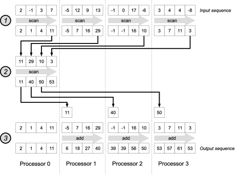
A somewhat simpler algorithm for computing prefix sums of $N$ items with $P$ processors in time $O(N/P+P)$ is illustrated in Figure 7; in the figure we consider the addition operator, although the idea applies to any associative operator $\oplus$. The computation involves two parallel steps (steps \raisebox{-.9pt} {\sf1}⃝ and \raisebox{-.9pt} {\sf3}⃝ in the figure), and one serial step (step \raisebox{-.9pt} {\sf2}⃝). In step \raisebox{-.9pt} {\sf1}⃝ the input sequence is split across the processors, and each processor computes the prefix sum of the elements in its portion. In step \raisebox{-.9pt} {\sf2}⃝ the master computes the prefix sum of the $P$ last local sums. Finally, in step \raisebox{-.9pt} {\sf3}⃝ the master scatters the first $(P-1)$ computed values (prefix sums of the last local sums) to the last $(P-1)$ processors. Each processor, except the first one, adds (more precisely, applies the $\oplus$ operator) the received value to the prefix sums from step \raisebox{-.9pt} {\sf1}⃝, producing a portion of the output sequence.

Steps \raisebox{-.9pt} {\sf1}⃝ and \raisebox{-.9pt} {\sf3}⃝ require time $O(N/P)$ each, while step \raisebox{-.9pt} {\sf2}⃝ is executed by the master in time $O(P)$, yielding a total time $O(N/P+P)$. Therefore, the algorithm is optimal when $N>P^{2}$. Since the current generation of CPUs have a small number of cores (e.g., $P\leq 72$ for the Intel Xeon Phi) and the number of regions $N$ is usually very large, the algorithm above can be considered optimal for any practical purpose. We remark that the parallel SBM algorithm can be readily implemented with the tree-structured reduction operation, and therefore will still be competitive on future generations of processors with a higher number of cores.

Algorithm 7 $\langle$Initialize $\texttt{SubSet}[0..P\!-\!1]$ and $\texttt{UpdSet}[0..P\!-\!1]\rangle$

1:for $p\leftarrow 0~{}\textrm{to}~{}P-1$ in parallel do$\triangleright$ Executed by all processors in parallel

2:     $\texttt{Sadd}[p]\leftarrow\emptyset$, $\texttt{Sdel}[p]\leftarrow\emptyset$, $\texttt{Uadd}[p]\leftarrow\emptyset$, $\texttt{Udel}[p]\leftarrow\emptyset$

3:     for all points $t\in T_{p}$ in non-decreasing order do

4:         if $t$ belongs to subscription region $s$ then

5:              if $t$ is the lower bound of $S_{i}$ then

6:                  $\texttt{Sadd}[p]\leftarrow\texttt{Sadd}[p]\cup\{s\}$

7:              else if $s\in\texttt{Sadd}[p]$ then

8:                  $\texttt{Sadd}[p]\leftarrow\texttt{Sadd}[p]\setminus\{s\}$

9:              else

10:                  $\texttt{Sdel}[p]\leftarrow\texttt{Sdel}[p]\cup\{s\}$               

11:         else$\triangleright$ $t$ belongs to update region $u$

12:              if $t$ is the lower bound of $u$ then

13:                  $\texttt{Uadd}[p]\leftarrow\texttt{Uadd}[p]\cup\{u\}$

14:              else if $u\in\texttt{Uadd}[p]$ then

15:                  $\texttt{Uadd}[p]\leftarrow\texttt{Uadd}[p]\setminus\{u\}$

16:              else

17:                  $\texttt{Udel}[p]\leftarrow\texttt{Udel}[p]\cup\{u\}$                             

18:$\triangleright$ Executed by the master only

19:$\texttt{SubSet}[0]\leftarrow\emptyset$, $\texttt{UpdSet}[0]\leftarrow\emptyset$

20:for $p\leftarrow 1~{}\textrm{to}~{}P-1$ do

21:     $\texttt{SubSet}[p]\leftarrow\texttt{SubSet}[p-1]\cup\texttt{Sadd}[p-1]\setminus\texttt{Sdel}[p-1]$

22:     $\texttt{UpdSet}[p]\leftarrow\texttt{UpdSet}[p-1]\cup\texttt{Uadd}[p-1]\setminus\texttt{Udel}[p-1]$

Figure 8. Parallel prefix computation for the SBM algorithm.

Initialization with prefix computation

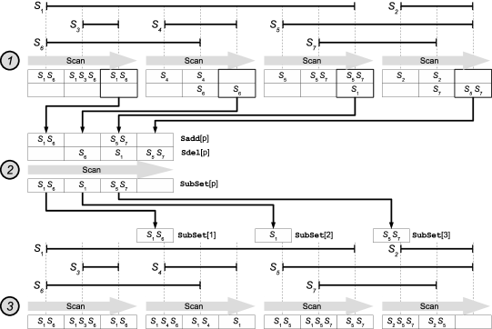
We can now complete the description of the parallel SBM algorithm by showing how the arrays $\texttt{SubSet}[p]$ and $\texttt{UpdSet}[p]$ can be initialized in parallel. To better illustrate the steps involved, we refer to the example in Figure 8; in the figure we consider subscription regions only, since the procedure for update regions is the same.

The sorted array of endpoints $T$ is evenly split into $P$ segments $T_{0},\ldots,T_{P-1}$ of $2\times(n+m)/P$ elements each. Processor $p$ scans the endpoints $t\in T_{p}$ in non-decreasing order, updating four auxiliary variables $\texttt{Sadd}[p]$, $\texttt{Sdel}[p]$, $\texttt{Uadd}[p]$, and $\texttt{Udel}[p]$. Informally, $\texttt{Sadd}[p]$ and $\texttt{Sdel}[p]$ (resp. $\texttt{Uadd}[p]$ and $\texttt{Udel}[p]$) contain the endpoints that the sequential SBM algorithm would add/remove from SubSet (resp. UpdSet) while scanning the endpoints belonging to segment $T_{p}$. More formally, at the end of each local scan the following invariants hold:

1. $\texttt{Sadd}[p]$ (resp. $\texttt{Uadd}[p]$) contains the subscription (resp. update) intervals whose lower endpoint belongs to $T_{p}$, and whose upper endpoint does not belong to $T_{p}$;

2. $\texttt{Sdel}[p]$ (resp. $\texttt{Udel}[p]$) contains the subscription (resp. update) intervals whose upper endpoint belongs to $T_{p}$, and whose lower endpoint does not belong to $T_{p}$.

This step is realized by lines 1–17 of Algorithm 7, and its effects are shown in Figure 8 \raisebox{-.9pt} {\sf1}⃝. The figure reports the values of $\texttt{Sadd}[p]$ and $\texttt{Sdel}[p]$ after each endpoint has been processed; the algorithm does not store every intermediate value, since only the last ones (within thick boxes) will be needed by the next step.

Once all $\texttt{Sadd}[p]$ and $\texttt{Sdel}[p]$ are available, the next step is executed by the master and consists of computing the values of $\texttt{SubSet}[p]$ and $\texttt{UpdSet}[p]$, $p=0,\ldots,P-1$. Recall from the discussion above that $\texttt{SubSet}[p]$ (resp. $\texttt{UpdSet}[p]$) is the set of active subscription (resp. update) intervals that would be identified by the sequential SBM algorithm right after the end of segment $T_{0}\cup\ldots\cup T_{p-1}$. The values of $\texttt{SubSet}[p]$ and $\texttt{UpdSet}[p]$ are related to $\texttt{Sadd}[p]$, $\texttt{Sdel}[p]$, $\texttt{Uadd}[p]$ and $\texttt{Udel}[p]$ as follows:

$$\texttt{SubSet}[p] =\begin{cases}\emptyset&\mbox{if $p=0$}\\ \texttt{SubSet}[p-1]\cup\texttt{Sadd}[p-1]\setminus\texttt{Sdel}[p-1]&\mbox{if $p>0$}\end{cases}$$

$$\texttt{UpdSet}[p] =\begin{cases}\emptyset&\mbox{if $p=0$}\\ \texttt{UpdSet}[p-1]\cup\texttt{Uadd}[p-1]\setminus\texttt{Udel}[p-1]&\mbox{if $p>0$}\end{cases}$$

Intuitively, the set of active intervals at the end of $T_{p}$ can be computed from those active at the end of $T_{p-1}$, plus the intervals that became active in $T_{p}$, minus those that ceased to be active in $T_{p}$.

Lines 19–22 of Algorithm 7 take care of this computation; see also Figure 8 \raisebox{-.9pt} {\sf2}⃝ for an example. Once the initial values of $\texttt{SubSet}[p]$ and $\texttt{UpdSet}[p]$ have been computed, Algorithm 6 can be resumed to identify the list of overlaps.

Asymptotic execution time

We now analyze the asymptotic execution time of parallel SBM. Let $N$ denote the total number of subscription and update regions, and $P$ the number of processors. Algorithm 6 consists of three phases:

1. Sorting $T$ in non-decreasing order requires total time $O\left((N\lg N)/P\right)$ using a parallel sorting algorithm such as parallel mergesort (Cole, 1988).

2. Computing the initial values of $\texttt{SubSet}[p]$ and $\texttt{UpdSet}[p]$ for each $p=0,\ldots,P-1$ requires $O\left(N/P+P\right)$ steps using the two-level scan shown on Algorithm 7; the time could be reduced to $O\left(N/P+\lg P\right)$ steps using the tree-structured scan by Blelloch (Blelloch, 1989).

3. Each of the final local scans require $O(N/P)$ steps.

Note, however, that phases 2 and 3 require the manipulation of data structures to store sets of endpoints, supporting insertions and removals of single elements and whole sets. Therefore, a single step of the algorithm has a non-constant time complexity that depends on the actual implementation of sets and the number of elements they contain; this issue will be discussed in more detail in Section 5. During phase 3 total time $O(K)$ is spent cumulatively by all processors to report all $K$ intersections.

Some remarks on distributed-memory and GPU implementations

Although the focus of this paper is on shared-memory architectures, we provide here some remarks on possible distributed-memory and GPU implementations of Algorithm 6.

In a distributed-memory system, computing nodes exchange information through some type of high-performance network connection. It turns out that a distributed-memory implementation of Algorithm 6 can be realized with minimal modifications. First, a suitable distributed-memory sorting algorithm (e.g., (Solomonik and Kalé, 2010)) can be used to sort the list of endpoints. Then, the parallel prefix computation shown in Figure 8 can be realized efficiently since it is based on the Scatter/Gather communication pattern (Mattson et al., 2004). A Scatter operation allows a single process to send portions of a local array to multiple destinations, and is executed between steps \raisebox{-.9pt} {\sf2}⃝ and \raisebox{-.9pt} {\sf3}⃝ in Figure 8. The symmetric Gather allows multiple processes to send portions of an array to a single destination where they are concatenated; this is required between steps \raisebox{-.9pt} {\sf1}⃝ and \raisebox{-.9pt} {\sf2}⃝. Since Scatter/Gather primitives are very useful in many contexts, they are efficiently supported by software middlewares (e.g., the MPI_Scatter() MPI_Gather() functions of the Message Passing Interface specification), or directly at the hardware level (Almási et al., 2005).

An efficient GPU implementation of Algorithm 6, however, poses several challenges. Although GPU-based efficient algorithms for sorting and doing prefix computations are available (Bell and Hoberock, 2012), the data structure used to represent sets of endpoints must be designed carefully. As described earlier in this Section, Algorithm 6 performs $\Theta(N)$ set operations (unions and differences) during the prefix computation, and therefore the data structure used for representing sets must be chosen wisely (we will return to this issue in Section 5). Data structures based on hash tables or trees are problematic on the GPU, although not impossible (Awad et al., 2019; Ashkiani et al., 2018). A simpler implementation of sets using bit vectors appears to be better suited: a bit vector is a sequence of $N$ bits, where item $i$ is in the set if and only if the $i$-th bit is one. Bit vectors allow union, intersection and set difference to be realized efficiently using nothing more than Boolean operators; however, bit vectors require considerable amounts of memory if the number $N$ of items that could be in the set is large. This issue requires further investigation, and is subject of ongoing research.

5. Experimental Evaluation

In this section we evaluate the performance and scalability of the parallel ITM and parallel SBM algorithms, and compare them to parallel implementations of BFM and GBM. BFM and ITM have been implemented in C, while SBM and GBM have been implemented in C++. To foster the reproducibility of our experiments, all the source code used in this performance evaluation is freely available on the research group website (pad, 2018) with a Free Software license.

We used the GNU C Compiler (GCC) version 4.8.4 with the -O3 -fopenmp -D_GLIBCXX_PARALLEL flags to turn on optimization and to enable parallel constructs at the compiler and library levels. Specifically, the -fopenmp flag instructs the compiler to handle OpenMP directives in the source code (Dagum and Menon, 1998), while the flag -D_GLIBCXX_PARALLEL enables parallel implementations of some algorithms from the C++ Standard Template Library (STL) to be used instead of their sequential counterparts (more details below).

OpenMP is an open interface supporting shared memory parallelism in the C, C++ and FORTRAN programming languages. OpenMP allows the programmer to label specific sections of the source code as parallel regions; the compiler takes care of dispatching these regions to different threads that can be executed by the available processors or cores. In the C/C++ languages, OpenMP directives are specified using #pragma directives. The OpenMP standard also defines some library functions that can be called by the developer to query and control the execution environment programmatically.

The BFM and ITM algorithms are embarrassingly parallel, meaning that the iterations on their main loop (line 1 on Algorithm 2 and line 11 on Algorithm 5) are free of data races. Therefore, a single #pragma omp parallel for directive is sufficient to distribute the iterations of the loops across the processors.

GBM requires more care, as we have already observed in Section 2, since the first loop (lines 6–10, Algorithm 3) has a data race due to possible concurrent updates to the list $G[i]$ in line 9. A simple solution consists on protecting the statement with a #pragma omp critical directive that ensures that only one thread at a time can modify a list. However, this might limit the degree of parallelism since two OpenMP threads would be prevented from updating two different lists concurrently. To investigate this issue we developed an ad-hoc, lock-free linked list data structure that supports concurrent append operations without the need to declare a critical section. Measurements showed that in our experiments the ad-hoc linked list did not perform significantly better, so we decided to use the standard std::list container provided by the C++  Standard Template Library (STL) library (Stroustrup, 2013), and protect concurrent updates with the OpenMP critical directive.

Our implementation of parallel SBM relies on some of the data structures and algorithms provided by the C++ STL. Specifically, to sort the endpoints we use the parallel std::sort function provided by the STL extensions for parallelism (C++, 2015). Indeed, the GNU STL provides several parallel sort algorithms (multiway mergesort and quicksort with various splitting heuristics) that are automatically selected at compile time when the -D_GLIBCXX_PARALLEL compiler flag is used. The rest of the SBM algorithm has been parallelized using explicit OpenMP parallel directives.

The  Sort-based Matching (SBM) algorithm relies on a suitable data structure to store the sets of endpoints SubSet and UpdSet (see Algorithms 6 and 7). Parallel SBM puts a higher strain on this data structure than its sequential counterpart, since it also requires efficient support for unions and differences between sets, in addition to insertions and deletions of single elements. We have experimented with several implementations for sets: (i) bit vectors based on the std::vector<bool> STL container; (ii) an ad-hoc implementation of bit vectors based on raw memory manipulation; (iii) the std::set container, that in the case of the GNU STL is based on Red-Black trees (Bayer, 1972); (iv) the std::unordered_set container from the 2011 ISO C++ standard, that is usually implemented using hash tables; (v) the boost::dynamic_bitset container provided by the Boost C++ library (boo, 2019). The most efficient turned out to be the std::set container, and it has been used in the experiments described below.

CPU	Intel Xeon E5-2640
Clock frequency	2.00 GHz
Processors	2
Cores/proc	8
Total cores	16
Threads/core	2
HyperThreading	Yes
RAM	128 GB
L3 cache size	20480 KB
Operating System	Ubuntu 16.04.3 LTS

Table 1. Hardware used for the experimental evaluation.

Experimental setup

The experiments below have been carried out on a dual-socket, octa-core server whose hardware specifications are shown in Table 1. The processors employ the  Hyper-Threading (HT) technology (Marr et al., 2002): in HT-enabled CPUs some functional components are duplicated, but there is a single main execution unit for physical core. From the point of view of the  Operating System (OS), HT provides two logical processors for each physical core. Studies from Intel and others have shown that in typical applications HT contributes a performance boost in the range $16$–$28\%$ (Marr et al., 2002). When two processes are executed on the same core, they compete for the shared hardware resources resulting is lower efficiency than the same two processes executed on two different physical cores.

The number $P$ of OpenMP threads to use can be chosen either programmatically through the appropriate OpenMP functions, or setting the OMP_NUM_THREADS environment variable. In our experiments, $P$ never exceeds the total number of (logical) cores, so that over-provisioning never happens. By default, the Linux scheduler spreads processes to different physical cores as long as possible; only when there are more runnable processes than physical cores does HT come into effect. All tests have been executed with this default behavior.

For better comparability of our results with those in the literature, we consider $d=1$ dimensions and use the methodology and parameters described in (Raczy et al., 2005) (a performance evaluation based on real dataset will be described at the end of this section). The first parameter is the total number of regions $N$, that includes $n=N/2$ subscription and $m=N/2$ update regions. All regions have the same length $l$ and are randomly placed on a segment of total length $L=10^{6}$. $l$ is defined in such a way that a given overlapping degree $\alpha$ is obtained, where

$$\alpha=\frac{\sum\text{area of regions}}{\text{area of the routing space}}=\frac{N\times l}{L}$$

Therefore, given $\alpha$ and $N$, the value of $l$ is set to $l=\alpha L/N$. The overlapping degree is an indirect measure of the total number of intersections among subscription and update regions. While the performance of BFM and SBM is not affected by the number of intersections, this is not the case for ITM, as will be shown below. We considered the same values for $\alpha$ as in (Raczy et al., 2005), namely $\alpha\in\{0.01,1,100\}$. Finally, each measure is the average of $50$ independent runs to get statistically valid results. Our implementations do not explicitly store the list of intersections, but only count them. We did so to ensure that the execution times are not affected by the choice of the data structure used to store the list of intersections.

(a) Wall-clock time

(b) Speedup

Figure 9. Wall clock time and speedup of parallel {BFM, GBM, ITM, SBM} with $N=10^{6}$ regions and overlapping degree $\alpha=100$; the GBM algorithm uses $3000$ regions. Dashed lines indicate the region where the number of OpenMP threads exceeds the number of (physical) CPU cores.

Wall clock time and Speedup

The first metric we analyze is the  Wall Clock Time (WCT) of the parallel programs. The WCT includes the time needed to initialize all ancillary data structures used by each algorithm (e.g., the time needed to build the interval tree, or to fill the grid cells), but does not include the time required to randomly initialize the input regions.

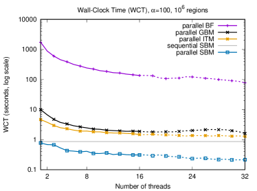
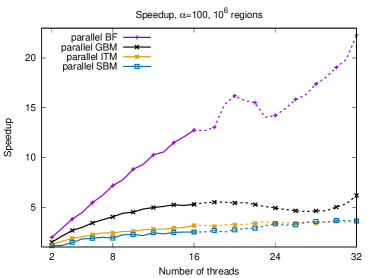
Figure 9(a) shows the WCT for the parallel versions of BFM, GBM, ITM and SBM as a function of the number $P$ of OpenMP threads, given $N=10^{6}$ regions and overlapping degree $\alpha=100$. The GBM algorithm requires the user to define the number of grid blocks ($\mathit{nblocks}$) to use. This parameter should be carefully chosen since it affects the algorithm’s performance (Tan et al., 2000a). We have empirically determined that the best running time with $P=32$ OpenMP threads with the parameters above is $3000$ regions. Dashed lines indicate when $P$ exceeds the number of physical cores.

We observe that the parallel BFM algorithm is about three orders of magnitude slower than parallel SBM. This is unsurprising, since the computational cost of BFM grows quadratically with the number of regions (see Section 2), while that of SBM and ITM grows only polylogarithmically. SBM performs better than BFM by almost two orders of magnitude. ITM is faster than BFM (remember that Figure 9(a) uses a logarithmic scale), and provides the additional advantage of requiring no tuning of parameters.

A drawback of GBM is that it requires the number of grid cells to be defined. The optimal value depends both on the simulation model and also on the number of OpenMP threads $P$; our chosen value ($3000$ regions) is optimal for $P=32$, but not necessarily for the other values of $P$; indeed, we observe that the execution time of parallel GBM increases around $P=24$; this shows up as a prominent feature in the speedup graph as explained below.

The relative speedup measures the increase in speed that a parallel program achieves when more processors are employed to solve a problem of the same size. This metric can be computed from the WCT as follows. Let $T(N,P)$ be the WCT required to process an input of size $N$ using $P$ processes (OpenMP threads). Then, for a given $N$, the relative speedup $S_{N}(P)$ is defined as $S_{N}(P)=T(N,1)/T(N,P)$. Ideally, the maximum value of $S_{N}(P)$ is $P$, which means that solving a problem with $P$ processors requires $1/P$ the time needed by a single processor. In practice, however, several factors limit the speedup, such as the presence of serial regions in the parallel program, uneven load distribution, scheduling overhead, and heterogeneity in the execution hardware.

Figure 9(b) shows the speedups of the parallel versions of BFM, GBM, ITM and SBM as a function of the number of OpenMP threads $P$; the speedup has been computed using the wall clock times of Figure 9(a). Again, dashed lines indicate data points where $P$ exceeds the number of physical processor cores. The BFM algorithm, despite being the less efficient, is the most scalable due to its embarrassingly parallel structure and lack of any serial part. SBM, on the other hand, is the most efficient but less scalable. SBM achieves a $2.6\times$ speedup with $16$ OpenMP threads. When all “virtual” cores are used, the speedup grows to $3.6\times$. The limited scalability of SBM is somewhat to be expected, since its running time is very small and therefore the overhead introduced by OpenMP becomes non-negligible.

The effect of HT (dashed lines) is clearly visible in Figure 9(b). The speedup degrades when $P$ exceeds the number of cores, as can be seen from the different slopes for BFM on titan. When HT kicks in, load unbalance arises due to contention of the shared control units of the processor cores, and this limits the scalability. The curious “bulge” that appears on the curve is due to some OpenMP scheduling issues on the machine used for the test, that is based on a  Non Uniform Memory Access (NUMA) architecture (Broquedis et al., 2008). Indeed, the bulge appears even if we replace the body of the inner loop of the BFM algorithm (line 3 of algorithm 2) with a dummy statement; moreover, the bulge does not appear if we run the BFM algorithm on a non-NUMA machine.

(a) Wall-clock time

(b) Speedup

Figure 10. Wall clock time and speedup of parallel {ITM, SBM} with $N=10^{8}$ regions and overlapping degree $\alpha=100$. Dashed lines indicate the region where the number of OpenMP threads exceeds the number of CPU cores, and therefore HT comes into play.

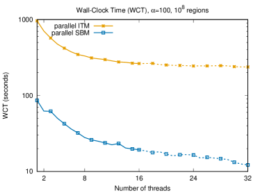
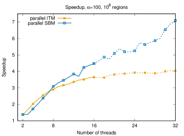
The speedup of SBM improves if we increase the work performed by the algorithm. Figure 10(b) shows the speedup of parallel ITM and SBM with $N=10^{8}$ regions and overlapping degree $\alpha=100$; in this scenario both BFM and GBM take so long that they have been omitted. The SBM algorithm behaves better, achieving a $7\times$ speedup with $P=32$ threads. The reason of this improvement is that increasing the amount of work executed by each processor reduces the synchronization overhead, which is particularly beneficial on multi-socket NUMA machines.

Figure 11. Wall clock time of parallel GBM with $N=10^{6}$ regions and overlapping degree $\alpha=100$. For each value of the number of OpenMP threads $P$, a red dot indicates the number of grid cells minimizing the WCT. Each WCT is the average of $50$ measurements.

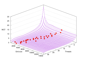
We have said above that the optimum number of grid cells in the parallel GBM algorithm depends on the number of OpenMP threads $P$. Figure 11 shows this dependency for a scenario with $N=10^{6}$ regions and overlapping degree $\alpha=100$. In the figure we report the WCT as a function of $P$ and of the number of grid cells; for each value of $P$ we put a red dot on the combination of parameters that provides the minimum WCT. As we can see, the optimum number of grid cells changes somewhat erratically as $P$ increases, although it shows a clear trend suggesting that a larger number of cells is better for low values of $P$, while a small number of cells is better for high values of $P$. A more precise characterization of the WCT of the parallel GBM algorithm would be an interesting research topic, that however falls outside the scope of the present paper.

(a)

(b)

Figure 12. Wall clock time of parallel ITM and SBM as a function of the number of regions $N$ (a) and overlapping degree $\alpha$ (b) (logarithmic horizontal scale).

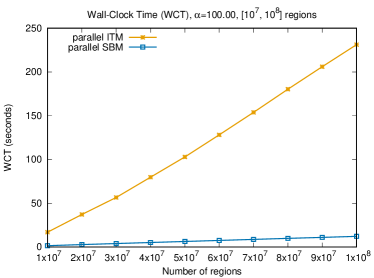
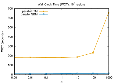
We now turn our attention on how the WCT changes as a function of the number of regions $N$, and as a function of the overlapping degree $\alpha$. We set the number of OpenMP threads to $P=32$, the number of logical cores provided by the test machine. Figure 12(a) shows the WCT of parallel ITM and SBM for $\alpha=100$, by varying the number of regions $N$ in the range $[10^{7},10^{8}]$. In this range both BFM and GBM require a huge amount of time, that is orders of magnitude higher than those of ITM and SBM, and will therefore be omitted from the comparison. From the figure we observe that the execution times of both ITM and SBM grow polylogarithmically with $N$, supporting the asymptotic analysis in Section 4; however, parallel SBM is faster than ITM, suggesting that its asymptotic cost has smaller constant factors.

In Figure 12(b) we report the WCT as a function of $\alpha$, for a fixed $N=10^{8}$. We observe that, unlike ITM, the execution time of SBM is essentially independent from the overlapping degree.

(a)

(b)

Figure 13. Memory usage (peak resident set size, VmHWM) of parallel BFM, GBM, ITM and SBM with an increasing number of regions (a) or threads (b), overlapping degree $\alpha=100$.

Memory Usage

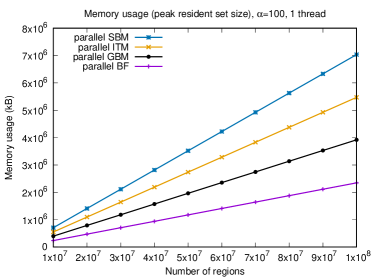
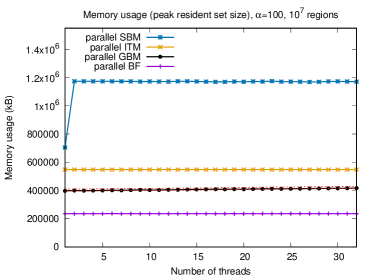
We conclude our experimental evaluation with an assessment of the memory usage of the parallel BFM, GBM, ITM and SBM algorithms. Figure 13 shows the peak  Resident Set Size (RSS) of the four algorithms as a function of the number of regions $N$ and OpenMP threads $P$, respectively. The RSS is the portion of a process memory that is kept in RAM. Care has been taken to ensure that all experiments reported in this section fit comfortably in the main memory of the available machines, so that the RSS represents an actual upper bound of the amount of memory required by the algorithms. Note that the data reported in Figure 13 includes the code for the test driver and the input arrays of intervals.

Figure 13(a) shows that the resident set size grows linearly with the number of regions $N$ for all algorithms. BFM has the smaller memory footprint, which is expected since it requires a small bounded amount of additional memory for a few local variables. On the other hand, SBM requires the highest amount of memory of the four algorithms, since it allocates larger data structures, namely the list of endpoints to be sorted, and a few arrays of sets that are used during the scan phase. In our tests, SBM requires approximately $7$ GB of memory to process $N=10^{8}$ intervals, about three times the amount of memory required by BFM.

In Figure 13(b) we see that the RSS does not change as the number of OpenMP threads $P$ increases, with overlapping degree $\alpha=100$ and $N=10^{6}$ regions. The anomaly shown by SBM going from $P=1$ to $P=2$ is due to the OpenMP runtime system.

(a) Wall-clock time

(b) Speedup

Figure 14. Wall clock time and speedup of parallel { GBM, ITM, SBM} with the Koln dataset; the GBM algorithm uses $3000$ grid cells. Dashed lines indicate the region where the number of OpenMP threads exceeds the number of (physical) CPU cores.

Performance Evaluation with the Koln Dataset

So far we have evaluated the DDM implementations using a synthetic workload. We now complement the analysis by considering a more realistic workload taken from the vehicular mobility research domain. Specifically, we use the Cologne dataset (Uppoor and Fiore, 2011), a realistic (although synthetic) trace of car traffic in the city of Cologne, Germany. The complete dataset contains the timestamped positions of more than $700.000$ vehicles moving on the greater urban area of Cologne ($400$ square kilometers) over a period of $24$ hours.

We consider a portion of the dataset that includes $541,222$ positions. The $x$ coordinate of each position is used as the center of one subscription and one update region; therefore, there are about $N=10^{6}$ regions overall. The width of each region is set to $100$ meters, resulting in approximately $3.9\times 10^{9}$ intersections.

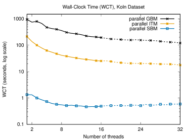
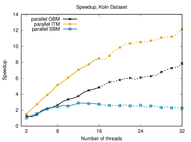
Figure 14 shows the WCT and speedup of the parallel versions of the GBM, ITM and SBM algorithms; for GBM we used $3000$ grid cells. As usual, each data point is the average of $50$ independent runs. We observe that the parallel GBM algorithm is the slowest of the three, while parallel SBM is the fastest by a wide margin (three orders of magnitude faster than SBM, two orders of magnitude faster than ITM). Since SBM is very fast on this benchmark, its poor scalability is caused by the parallelization overhead of OpenMP that has a higher impact on low wall-clock times.

6. Conclusions

In this paper we described and analyzed two parallel algorithms for the region matching problem on shared-memory architectures. The region matching problem consists of enumerating all intersections among two sets of subscription and update regions; a region is a $d$-dimensional, iso-oriented rectangle. The region matching problem is at the core of the Data Distribution Management service which is part of the High Level Architecture.

The region matching problem in $d$ dimensions can be reduced to the simpler problem of computing intersections among one-dimensional segments. The first parallel solution to the 1D matching problem, called ITM, is based on an interval tree data structure. An interval tree is a binary balanced search tree that can store a set of segments, and can be used to efficiently enumerate all intersections with a given query segment. Once built, an interval tree can be efficiently queried in parallel. The second solution is based on a parallel extension of SBM, a state-of-the-art solution to the DDM problem.

We have implemented the parallel versions of ITM and SBM using the C/C++ programming languages with OpenMP extensions. These algorithms have been compared with parallel implementations of the Brute-Force and Grid-Based matching algorithms. The results show that the parallel versions of ITM and SBM are orders of magnitude faster than (the parallel versions of) Brute-Force and Grid-Based matching. Among the four algorithms considered, parallel SBM is the fastest in all scenarios we have examined. The ITM algorithm, while slower than SBM, can be easily extendable to cope with dynamic regions since the interval tree allows efficient insertion and deletion of regions. In fact, a version of SBM that can efficiently handle region updates has already been proposed (Pan et al., 2011), but it can not be readily adapted to the parallel version of SBM discussed in this paper. Developing a parallel and dynamic version of SBM is the subject of ongoing research.

In this paper we focused on shared-memory architectures, i.e., multicore processors, since they are virtually ubiquitous and well supported by open, standard programming frameworks (OpenMP). Modern GPUs can be faster than contemporary CPUs, and are increasingly being exploited for compute-intensive applications. Unfortunately, the parallel ITM and SBM algorithms presented in this paper are ill-suited for implementations on GPUs, since they rely on data structures with irregular memory access patterns and/or frequent branching within the code. Reworking the implementation details of ITM and SBM to better fit the Symmetric Multithreading model of modern GPUs is still and open problem that requires further investigation.

Appendix A Notation

$\mathbf{S}$	Subscription set $\mathbf{S}=\{S_{1},\ldots,S_{n}\}$
$\mathbf{U}$	Update set $\mathbf{U}=\{U_{1},\ldots,U_{m}\}$
$n$	Number of subscription regions
$m$	Number of update regions
$N$	Number of subscription and update regions ($N=n+m$)
$K_{s}$	N. of intersections of subscription region $s$ with all update regions ($0\leq K_{s}\leq m$)
$K_{u}$	N. of intersections of update region $u$ with all subscription regions ($0\leq K_{u}\leq n$)
$K$	Total number of intersections ($0\leq K\leq n\times m$)
$\alpha$	Overlapping degree ($\alpha>0$)
$P$	Number of processors

Appendix B Acronyms

References

- (1)
- HLA (2010a) 2010a. IEEE Standard for Modeling and Simulation (M&S) High Level Architecture (HLA)–Federate Interface Specification. IEEE Std 1516.1-2010 (Rev. of IEEE Std 1516.1-2000). (2010). https://doi.org/10.1109/IEEESTD.2010.5954120
- HLA (2010b) 2010b. IEEE Standard for Modeling and Simulation (M&S) High Level Architecture (HLA)–Framework and Rules. IEEE Std 1516-2010 (Rev. of IEEE Std 1516-2000). (2010). https://doi.org/10.1109/IEEESTD.2010.5553440
- HLA (2010c) 2010c. IEEE Standard for Modeling and Simulation (M&S) High Level Architecture (HLA)–Object Model Template (OMT) Specification. IEEE Std 1516.2-2010 (Rev. of IEEE Std 1516.2-2000). (2010). https://doi.org/10.1109/IEEESTD.2010.5557731
- pad (2018) 2018. Parallel And Distributed Simulation (PADS) research group. http://pads.cs.unibo.it. (2018).
- boo (2019) 2019. Boost C++ libraries. https://www.boost.org/. (2019).
- Abraham et al. (2015) Mark James Abraham, Teemu Murtola, Roland Schulz, Szilárd Páll, Jeremy C. Smith, Berk Hess, and Erik Lindahl. 2015. GROMACS: High performance molecular simulations through multi-level parallelism from laptops to supercomputers. SoftwareX 1-2 (2015), 19–25. https://doi.org/10.1016/j.softx.2015.06.001
- Adelson-Velskii and Landis (1962) G. Adelson-Velskii and E. M. Landis. 1962. An Algorithm for the Organization of Information. Doklady Akademii Nauk USSR 146, 2 (1962), 263–266.
- Almási et al. (2005) George Almási, Charles Archer, José G. Castaños, John A. Gunnels, C. Christopher Erway, Philip Heidelberger, Xavier Martorell, José E. Moreira, Kurt W. Pinnow, Joe Ratterman, Burkhard D. Steinmacher-Burow, William Gropp, and Brian R. Toonen. 2005. Design and implementation of message-passing services for the Blue Gene/L supercomputer. IBM Journal of Research and Development 49, 2-3 (2005), 393–406. https://doi.org/10.1147/rd.492.0393
- Ashkiani et al. (2018) S. Ashkiani, M. Farach-Colton, and J. D. Owens. 2018. A Dynamic Hash Table for the GPU. In 2018 IEEE International Parallel and Distributed Processing Symposium (IPDPS). 419–429. https://doi.org/10.1109/IPDPS.2018.00052
- Awad et al. (2019) Muhammad A. Awad, Saman Ashkiani, Rob Johnson, Martín Farach-Colton, and John D. Owens. 2019. Engineering a High-performance GPU B-Tree. In Proceedings of the 24th Symposium on Principles and Practice of Parallel Programming (PPoPP ’19). ACM, New York, NY, USA, 145–157. https://doi.org/10.1145/3293883.3295706
- Bayer (1972) Rudolf Bayer. 1972. Symmetric binary B-Trees: Data structure and maintenance algorithms. Acta Informatica 1, 4 (1972), 290–306. https://doi.org/10.1007/BF00289509
- Bell and Hoberock (2012) Nathan Bell and Jared Hoberock. 2012. Chapter 26 - Thrust: A Productivity-Oriented Library for CUDA. In GPU Computing Gems Jade Edition, Wen mei W. Hwu (Ed.). Morgan Kaufmann, Boston, 359–371. https://doi.org/10.1016/B978-0-12-385963-1.00026-5
- Bentley and Ottmann (1979) J. L. Bentley and T. A. Ottmann. 1979. Algorithms for Reporting and Counting Geometric Intersections. IEEE Trans. Comput. 28, 9 (Sept. 1979), 643–647. https://doi.org/10.1109/TC.1979.1675432
- Bentley and Wood (1980) Jon Louis Bentley and Derick Wood. 1980. An Optimal Worst Case Algorithm for Reporting Intersections of Rectangles. IEEE Trans. Comput. C-29, 7 (July 1980), 571–577. https://doi.org/10.1109/TC.1980.1675628
- Blelloch (1989) Guy E. Blelloch. 1989. Scans as primitive parallel operations. IEEE Trans. Comput. 38, 11 (Nov 1989), 1526–1538. https://doi.org/10.1109/12.42122
- Boukerche et al. (2005) A. Boukerche, N. J. McGraw, C. Dzermajko, and Kaiyuan Lu. 2005. Grid-filtered region-based data distribution management in large-scale distributed simulation systems. In 38th Annual Simulation Symposium. 259–266. https://doi.org/10.1109/ANSS.2005.23
- Boukerche and Roy (2002) Azzedine Boukerche and Amber Roy. 2002. Dynamic Grid-Based Approach to Data Distribution Management. J. Parallel and Distrib. Comput. 62, 3 (2002), 366 – 392. https://doi.org/10.1006/jpdc.2001.1799
- Broquedis et al. (2008) François Broquedis, François Diakhaté, Samuel Thibault, Olivier Aumage, Raymond Namyst, and Pierre-André Wacrenier. 2008. Scheduling Dynamic OpenMP Applications over Multicore Architectures. In OpenMP in a New Era of Parallelism: 4th International Workshop, IWOMP 2008 West Lafayette, IN, USA, May 12-14, 2008 Proceedings, Rudolf Eigenmann and Bronis R. de Supinski (Eds.). Springer Berlin Heidelberg, Berlin, Heidelberg, 170–180. https://doi.org/10.1007/978-3-540-79561-2_15
- Busato and Bombieri (2016) Federico Busato and Nicola Bombieri. 2016. An Efficient Implementation of the Bellman-Ford Algorithm for Kepler GPU Architectures. IEEE Transactions on Parallel and Distributed Systems 27, 8 (Aug. 2016), 2222–2233. https://doi.org/10.1109/TPDS.2015.2485994
- C++ (2015) C++ 2015. Programming Languages – Technical Specification for C++ Extensions for Parallelism. ISO/IEC TS 19570:2015. (2015).
- Cetin et al. (2002) Nurhan Cetin, Kai Nagel, Bryan Raney, and Andreas Voellmy. 2002. Large-scale multi-agent transportation simulations. Computer Physics Communications 147, 1 (2002), 559–564. https://doi.org/10.1016/S0010-4655(02)00353-3 Proceedings of the Europhysics Conference on Computational Physics Computational Modeling and Simulation of Complex Systems.
- Cole (1988) R. Cole. 1988. Parallel Merge Sort. SIAM J. Comput. 17, 4 (1988), 770–785. https://doi.org/10.1137/0217049
- Cormen et al. (2009) Thomas H. Cormen, Charles E. Leiserson, Ronald L. Rivest, and Clifford Stein. 2009. Introduction to Algorithms (3rd ed.). MIT Press. I–XIX, 1–1292 pages.
- Dagum and Menon (1998) Leonardo Dagum and Ramesh Menon. 1998. OpenMP: An Industry-Standard API for Shared-Memory Programming. IEEE Comput. Sci. Eng. 5 (January 1998), 46–55. Issue 1. https://doi.org/10.1109/99.660313
- D’Angelo and Marzolla (2014) Gabriele D’Angelo and Moreno Marzolla. 2014. New trends in parallel and distributed simulation: From many-cores to Cloud Computing. Simulation Modelling Practice and Theory 49 (2014), 320–335. https://doi.org/10.1016/j.simpat.2014.06.007
- Devai and Neumann (2010) Frank Devai and Laszlo Neumann. 2010. A Rectangle-Intersection Algorithm with Limited Resource Requirements. In Proc. 10th IEEE Int. Conf. on Computer and Information Technology (CIT ’10). IEEE Computer Society, Washington, DC, USA, 2335–2340. https://doi.org/10.1109/CIT.2010.402
- Edelsbrunner (1983) Herbert Edelsbrunner. 1983. A new approach to rectangle intersections – Part II. International Journal of Computer Mathematics 13, 3-4 (1983), 221–229. https://doi.org/10.1080/00207168308803365
- Eroglu et al. (2008) Omer Eroglu, H. Ali Mantar, and Fatih Erdogan Sevilgen. 2008. Quadtree-based Approach to Data Distribution Management for Distributed Simulations. In Proceedings of the 2008 Spring Simulation Multiconference (SpringSim ’08). Society for Computer Simulation International, San Diego, CA, USA, 667–674. http://dl.acm.org/citation.cfm?id=1400549.1400656
- Finkel and Bentley (1974) R. A. Finkel and J. L. Bentley. 1974. Quad trees a data structure for retrieval on composite keys. Acta Informatica 4, 1 (01 Mar 1974), 1–9. https://doi.org/10.1007/BF00288933
- Guibas and Sedgewick (1978) Leo J. Guibas and Robert Sedgewick. 1978. A dichromatic framework for balanced trees. In Foundations of Computer Science, 1978., 19th Annual Symposium on. 8–21. https://doi.org/10.1109/SFCS.1978.3
- Guttman (1984) Antonin Guttman. 1984. R-trees: a dynamic index structure for spatial searching. SIGMOD Rec. 14, 2 (June 1984), 47–57. https://doi.org/10.1145/971697.602266
- Hillis and Steele (1986) W. Daniel Hillis and Guy L. Steele, Jr. 1986. Data Parallel Algorithms. Commun. ACM 29, 12 (Dec. 1986), 1170–1183. https://doi.org/10.1145/7902.7903
- Jacob et al. (2004) Christian Jacob, Julius Litorco, and Leo Lee. 2004. Immunity Through Swarms: Agent-Based Simulations of the Human Immune System. In Artificial Immune Systems, Giuseppe Nicosia, Vincenzo Cutello, Peter J. Bentley, and Jon Timmis (Eds.). Springer Berlin Heidelberg, Berlin, Heidelberg, 400–412. https://doi.org/10.1007/978-3-540-30220-9_32
- Jun et al. (2002) Yu Jun, C. Raczy, and G. Tan. 2002. Evaluation of a sort-based matching algorithm for DDM. In Proceedings 16th Workshop on Parallel and Distributed Simulation. 62–69. https://doi.org/10.1109/PADS.2002.1004202
- Junghyun Ahn and Kim (2012) Changho Sung Junghyun Ahn and Tag Gon Kim. 2012. A binary partition-based matching algorithm for Data Distribution Management in a High-level Architecture-based distributed simulation. Simulation: Transactions of the Society for Modeling and Simulation International 88, 11 (Nov. 2012), 1350–1367. https://doi.org/10.1177/0037549712450628
- Klügl and Rindsfüser (2007) Franziska Klügl and Guido Rindsfüser. 2007. Large-Scale Agent-Based Pedestrian Simulation. In Proc. 5th German Conference on Multiagent System Technologies (MATES 2007), Paolo Petta, Jörg P. Müller, Matthias Klusch, and Michael Georgeff (Eds.). Springer Berlin Heidelberg, Berlin, Heidelberg, 145–156. https://doi.org/10.1007/978-3-540-74949-3_13
- Law (2009) Averill M. Law. 2009. How to Build Valid and Credible Simulation Models. In Proceedings of the 2009 Winter Simulation Conference (WSC’09), M. D. Rossetti, R. R. Hill, B. Johansson, A. Dunkin, and R. G. Ingalls (Eds.). Winter Simulation Conference, 24–33. https://doi.org/10.1109/WSC.2009.5429312
- Li et al. (2018) Tianlin Li, Wenjie Tang, Yiping Yao, and Feng Zhu. 2018. A Binary Search Enhanced Sort-based Interest Matching Algorithm. In Proceedings of the 2018 ACM SIGSIM Conference on Principles of Advanced Discrete Simulation (SIGSIM-PADS ’18). ACM, New York, NY, USA, 125–128. https://doi.org/10.1145/3200921.3200941
- Liu and Theodoropoulos (2009) Elvis S. Liu and Georgios K. Theodoropoulos. 2009. An Approach for Parallel Interest Matching in Distributed Virtual Environments. In Proceedings of the 2009 13th IEEE/ACM International Symposium on Distributed Simulation and Real Time Applications (DS-RT ’09). IEEE Computer Society, Washington, DC, USA, 57–65. https://doi.org/10.1109/DS-RT.2009.34
- Liu and Theodoropoulos (2013) Elvis S. Liu and Georgios K. Theodoropoulos. 2013. An analysis of parallel interest matching algorithms in distributed virtual environments. In 2013 Winter Simulations Conference (WSC). 2889–2901. https://doi.org/10.1109/WSC.2013.6721658
- Liu and Theodoropoulos (2014) Elvis S. Liu and Georgios K. Theodoropoulos. 2014. Interest Management for Distributed Virtual Environments: A Survey. ACM Comput. Surveys 46, 4, Article 51 (April 2014), 42 pages. https://doi.org/10.1145/2535417
- Liu and Andelfinger (2017) Xinhu Liu and Philipp Andelfinger. 2017. Time Warp on the GPU: Design and Assessment. In Proceedings of the 2017 ACM SIGSIM Conference on Principles of Advanced Discrete Simulation (SIGSIM-PADS ’17). ACM, New York, NY, USA, 109–120. https://doi.org/10.1145/3064911.3064912
- Liu et al. (2015) Yanbing Liu, Hongbo Sun, Wenhui Fan, and Tianyuan Xiao. 2015. A parallel matching algorithm based on order relation for HLA data distribution management. International Journal of Modeling, Simulation, and Scientific Computing 06, 02 (2015), 1540002. https://doi.org/10.1142/S1793962315400024
- Marr et al. (2002) Deborah T. Marr, Frank Binns, David L. Hill, Glenn Hinton, David A. Koufaty, Alan J. Miller, and Michael Upton. 2002. Hyper-Threading Technology Architecture and Microarchitecture. Intel Technology Journal 6, 1 (Feb. 2002).
- Marzolla et al. (2013) Moreno Marzolla, Gabriele D’Angelo, and Marco Mandrioli. 2013. A parallel data distribution management algorithm. In 2013 IEEE/ACM 17th International Symposium on Distributed Simulation and Real Time Applications (DS-RT). 145–152. https://doi.org/10.1109/DS-RT.2013.23
- Mattson et al. (2004) Timothy Mattson, Beverly Sanders, and Berna Massingill. 2004. Patterns for Parallel Programming (first ed.). Addison-Wesley Professional.
- McCreight (1985) Edward M. McCreight. 1985. Priority Search Trees. SIAM J. Comput. 14, 2 (1985), 257–276. https://doi.org/10.1137/0214021
- Naylor et al. (1990) Bruce Naylor, John Amanatides, and William Thibault. 1990. Merging BSP Trees Yields Polyhedral Set Operations. SIGGRAPH Comput. Graph. 24, 4 (Sept. 1990), 115–124. https://doi.org/10.1145/97880.97892
- Pan et al. (2011) Ke Pan, Stephen John Turner, Wentong Cai, and Zengxiang Li. 2011. A dynamic sort-based DDM matching algorithm for HLA applications. ACM Trans. Model. Comput. Simul. 21, 3, Article 17 (Feb. 2011), 17 pages. https://doi.org/10.1145/1921598.1921601
- Petty and Morse (2004) Mikel D. Petty and Katherine L. Morse. 2004. The computational complexity of the high level architecture data distribution management matching and connecting processes. Simulation Modelling Practice and Theory 12, 3 (2004), 217–237. https://doi.org/10.1016/j.simpat.2003.10.004 Modeling and Simulation of Distributed Systems and Networks.
- Petty and Mukherjee (1997) Mikel D. Petty and Amar Mukherjee. 1997. Experimental Comparison of -Rectangle Intersection Algorithms Applied to HLA Data Distribution. In Proceedings of the 1997 Distributed Simulation Symposium. 13–26.
- Raczy et al. (2005) C. Raczy, G. Tan, and J. Yu. 2005. A sort-based DDM matching algorithm for HLA. ACM Trans. Model. Comput. Simul. 15, 1 (Jan. 2005), 14–38. https://doi.org/10.1145/1044322.1044324
- Rao et al. (2013) D. Rao, X. Hu, and L. Wu. 2013. Performance analysis of parallel data distribution management in large-scale battlefield simulation. In Proceedings of 2013 3rd International Conference on Computer Science and Network Technology. 134–138. https://doi.org/10.1109/ICCSNT.2013.6967080
- Rosenberg (1985) J.B. Rosenberg. 1985. Geographical Data Structures Compared: A Study of Data Structures Supporting Region Queries. Computer-Aided Design of Integrated Circuits and Systems, IEEE Transactions on 4, 1 (1985), 53–67. https://doi.org/10.1109/TCAD.1985.1270098
- Six and Wood (1980) H. W. Six and D. Wood. 1980. The rectangle intersection problem revisited. BIT Numerical Mathematics 20, 4 (01 Dec 1980), 426–433. https://doi.org/10.1007/BF01933636
- Six and Wood (1982) H. W. Six and D. Wood. 1982. Counting and Reporting Intersections of -Ranges. IEEE Trans. Comput. 31, 3 (March 1982), 181–187. https://doi.org/10.1109/TC.1982.1675973
- Solomonik and Kalé (2010) E. Solomonik and L. V. Kalé. 2010. Highly scalable parallel sorting. In 2010 IEEE International Symposium on Parallel Distributed Processing (IPDPS). 1–12. https://doi.org/10.1109/IPDPS.2010.5470406
- Stroustrup (2013) Bjarne Stroustrup. 2013. The C++ Programming Language, 4th Edition. Addison-Wesley.
- Tan et al. (2000a) Gary Tan, Rassul Ayani, YuSong Zhang, and Farshad Moradi. 2000a. Grid-based data management in distributed simulation. In Proceedings 33rd Annual Simulation Symposium. 7–13. https://doi.org/10.1109/SIMSYM.2000.844895
- Tan et al. (2000b) Gary Tan, YuSong Zhang, and Rassul Ayani. 2000b. A Hybrid Approach to Data Distribution Management. In Proceedings of the Fourth IEEE International Workshop on Distributed Simulation and Real-Time Applications (DS-RT ’00). IEEE Computer Society, Washington, DC, USA, 55–. https://doi.org/10.1109/DISRTA.2000.874064
- Tsigas and Zhang (2003) Philippas Tsigas and Yi Zhang. 2003. A Simple, Fast Parallel Implementation of Quicksort and its Performance Evaluation on SUN Enterprise 10000. In 11th Euromicro Workshop on Parallel, Distributed and Network-Based Processing (PDP 2003), 5-7 February 2003, Genova, Italy. IEEE Computer Society, 372. https://doi.org/10.1109/EMPDP.2003.1183613
- Uppoor and Fiore (2011) S. Uppoor and M. Fiore. 2011. Large-scale urban vehicular mobility for networking research. In 2011 IEEE Vehicular Networking Conference (VNC). 62–69. https://doi.org/10.1109/VNC.2011.6117125
- Van Hook et al. (1996) Daniel J. Van Hook, Steven J. Rak, and James O. Calvin. 1996. Approaches to RTI implementation of HLA data distribution management services. In Proceedings of the 15th Workshop on Standards for the Interoperability of Distributed Simulations. Orlando, FL, 535–544.
- Wheat and Evans (1992) M. Wheat and D. J. Evans. 1992. An efficient parallel sorting algorithm for shared memory multiprocessors. Parallel Comput. 18, 1 (1992), 91–102. https://doi.org/10.1016/0167-8191(92)90114-M
- Wulf and McKee (1995) Wm. A. Wulf and Sally A. McKee. 1995. Hitting the Memory Wall: Implications of the Obvious. SIGARCH Comput. Archit. News 23, 1 (March 1995), 20–24. https://doi.org/10.1145/216585.216588