Bimodal probability density characterizes the elastic behavior of a semiflexible polymer in 2D under compression

Abstract

We explore the elastic behavior of a wormlike chain under compression in terms of exact solutions for the associated probability densities. Strikingly, the probability density for the end-to-end distance projected along the applied force exhibits a bimodal shape in the vicinity of the critical Euler buckling force of an elastic rod, reminiscent of the smeared discontinuous phase transition of a finite system. These two modes reflect the almost stretched and the S-shaped configuration of a clamped polymer induced by the compression. Moreover, we find a bimodal shape of the probability density for the transverse fluctuations of the free end of a cantilevered polymer as fingerprint of its semiflexibility. In contrast to clamped polymers, free polymers display a circularly symmetric probability density and their distributions are identical for compression and stretching forces.

I Introduction

Semiflexible polymers are abundant in nature and play a pivotal role for the mechanical properties of single cells Sackmann (1994). Examples of these biopolymers include filamentous actin Lieleg et al. (2010), microtubules Brangwynne et al. (2006), and intermediate filaments Nolting et al. (2014), which all constitute integral parts of cells and form the ingenious scaffold inside the cell, the cytoskeleton Bausch and Kroy (2006). Together, these filaments account for the cell shape and its ability to adapt dynamically to its environment, its mechanical and structural stability, cell motility, intracellular transport processes, and also cell division Brangwynne et al. (2006); Fletcher and Mullins (2010); Lieleg et al. (2010). As the interior of a cell is densely packed and crowded with macromolecules, the environment of these filaments becomes constrained and alters their elastic behavior drastically Nolting et al. (2014). Cytoskeletal polymers often form bundles or networks, which are cross-linked by a large variety of regulatory proteins, or accumulate in entangled solutions Amuasi et al. (2015); Carrillo et al. (2013); Huisman et al. (2008); Kroy and Frey (1996); MacKintosh et al. (1995); Plagge et al. (2016); Razbin et al. (2015); Storm et al. (2005). Already in the force-free case, single polymers experience stretching and compression forces induced by their surrounding network, and consequently the distance between two ends of a polymer, that are, for instance, fixed by cross-links, differs significantly form their contour length. In the presence of mechanical stresses these networks exhibit fascinating nonlinear behavior on larger, macroscopic scales Amuasi et al. (2015); Carrillo et al. (2013); Chaudhuri et al. (2007); Claessens et al. (2006); Huisman et al. (2008); Kroy and Frey (1996); MacKintosh et al. (1995); Plagge et al. (2016); Razbin et al. (2015); Storm et al. (2005), such as the stiffening of materials with increasing strain Carrillo et al. (2013), or the reversible stress-softening behavior of filamentous actin networks Chaudhuri et al. (2007).

There has been significant progresss in the recent past to elaborate the principles for the peculiar nonlinear elastic behvior Broedersz and MacKintosh (2014), yet the mechanisms still require further elucidation at different levels of coarse-graining. In particular, the macroscopic behavior strongly depends on its single components and the mechanical properties of single filaments serve as an essential input to fully understand the elasticity of networks Hugel and Seitz (2001). Already single semiflexible polymers respond sensitively to external forces and, thereby, exhibit peculiar stretching and bending behavior Baczynski et al. (2007); Broedersz and MacKintosh (2014); Ott et al. (1993); Razbin et al. (2016). Experimental methods, including optical Ashkin (1997); Mehta et al. (1999) and magnetic tweezers Gosse and Croquette (2002), transmission electron microscopy Kuzumaki and Mitsuda (2006), and acoustic Sitters et al. (2015) and atomic force spectroscopy Hugel and Seitz (2001); Janshoff et al. (2000), have been applied to measure in vitro the nonlinear force-extension relation of purified biopolymers, such as DNA  Bouchiat et al. (1999); Bustamante et al. (2000); Marko and Siggia (1995); Sitters et al. (2015) and actin filaments Liu and Pollack (2002), single molecules, e.g. titin Kellermayer et al. (1997) and collagen Sun et al. (2002), and also synthetic carbon nanotubes Kuzumaki and Mitsuda (2006). Yet, in striking contrast to flexible polymers, the probability distribution for the end-to-end distance of semiflexible polymers is expected to deviate significantly from a simple Gaussian behavior Wilhelm and Frey (1996), and, thus, the mean end-to-end distance is not necessarily a good indicator for the shape of the associated probability distribution. Consequently, the full probability distribution is required to obtain a more general characterization of the elasticity of semiflexible polymers. Experimentally, fluorescence videomicroscopy has already been applied to access the probability distribution for the end-to-end distance of force-free actin filaments Le Goff et al. (2002) and semiflexible polymers confined to microchannels Köster et al. (2005); Köster and Pfohl (2009), but permits in principle also to extract reliable information on the polymer configurations induced by external loads.

A widely used model to describe the elastic properties of semiflexible polymers is the celebrated wormlike chain model, also referred to as Kratky-Porod model Kratky and Porod (1949). The force-free behavior of a wormlike chain with free ends has been elaborated analytically for the end-to-end probability density in the weakly-bending approximation Wilhelm and Frey (1996) and, furthermore, evaluated numerically for polymers of arbitrary stiffness using an inverse (Fourier) Laplace transform Samuel and Sinha (2002); Mehraeen et al. (2008). In addition, the probability density for the transverse fluctuations of the free end of a cantilevered polymer has been extracted from computer simulations Lattanzi et al. (2004) and qualitatively confirmed by an approximate theory Benetatos et al. (2005) in 2D and computed formally exactly in 3D by inverting an infinite matrix Semeriyanov and Stepanow (2007). To explore the response of semiflexible polymers to external forces, we have recently provided exact expressions for the two lowest-order moments, namely, the force-extension relation and the susceptibility (i.e. the variance) Kurzthaler and Franosch (2017), thereby, complementing theoretical and simulation studies on the stretching behavior Prasad et al. (2005) and the response of single semiflexible polymers upon compression in the weakly-bending approximation Kroy and Frey (1996); Baczynski et al. (2007). The smearing of the classical Euler buckling instability by thermal fluctuations leads to a rapid decrease of the force-extension relation and a strongly peaked susceptibility, reminiscent of a smeared discontinuous phase transition in a finite system. To corroborate this scenario and to fully understand the behavior of a semiflexible polymer under compression, access to the full probability distribution for the end-to-end distance is required.

Here, we first provide analytic expressions for the characteristic function, i.e. the Fourier transform of the probability density, of force-free wormlike chains with clamped ends, one free and one clamped end (i.e. cantilevered), and free ends reflecting different experimental setups. The exact solutions then permit to evaluate numerically via an inverse Fourier transform the associated probability densities for the end-to-end distance projected along or transverse to the clamped ends of the polymer. Furthermore, we explore the behavior of semiflexible polymers with different bending rigidities under compression and tension and provide insights into the polymer configurations via the probability density for the end-to-end distance projected onto the direction of the applied force. We validate our analytic results with the mean force-extension relation and the associated variance, elaborated previously Kurzthaler and Franosch (2017). Moreover, we have performed simulations for selected parameter sets and exemplarily compared them to our exact theory.

II Wormlike chain model

To explore the elastic properties of a single semiflexible polymer we employ the well-established wormlike chain model (WLC model). Here, the bending energy of a wormlike chain Kratky and Porod (1949) is expressed by its squared curvature,

$$\mathcal{H}_{0} =\frac{\kappa}{2}\int_{0}^{L}\!\mathrm{d}s\ \left(\frac{\mathrm{d}\mathbf{u}(s)}{\mathrm{d}s}\right)^{2},$$ (1)

where $s$ denotes the arc length of the polymer, $L$ its contour length, and $\kappa$ the bending rigidity. Furthermore, $\mathbf{u}(s)=\mathrm{d}\mathbf{r}(s)/\mathrm{d}s$ is the tangent vector of the polymer along its contour $\mathbf{r}(s)$ with unit length, $|\mathbf{u}(s)|=1$, see Fig. 1. In the framework of statistical physics the corresponding partition sum $Z_{0}(\mathbf{u}_{L},L|\mathbf{u}_{0},0)$ for a clamped polymer with initial orientation $\mathbf{u}_{0}$ and final orientation $\mathbf{u}_{L}$ is formally obtained as a path integral of Boltzmann weights over all possible chain configurations, which obey the local inextensibility constraint $|\mathbf{u}(s)|=1$,

$$Z_{0}(\mathbf{u}_{L},L|\mathbf{u}_{0},0) =\int_{\mathbf{u}(0)=\mathbf{u}_{0}}^{\mathbf{u}(L)=\mathbf{u}_{L}}\mathcal{D}[\mathbf{u}(s)]\exp\left(-\frac{\mathcal{H}_{0}}{k_{\text{B}}T}\right).$$ (2)

Here, $k_{\text{B}}$ denotes the Boltzmann constant and $T$ is the temperature of the system. Although the Hamiltonian is quadratic the path integral cannot be solved by Gaussian integrals due to the local inextensibility constraint. Yet, an exact solution of the partition sum can be elabaroted by deriving the corresponding Fokker-Planck equation and solving it in terms of associated eigenfunctions. In particular, in 2D the partition sum can formally be expanded into Fourier modes Spakowitz et al. (2004), which naturally introduces the persistence length $\ell_{\text{p}}=2\kappa/k_{\text{B}}T$ as the decay length of the tangent-tangent correlations of the polymer. In 3D, where the solution of the partition sum can be formally achieved in spherical harmonics, the persistence length is given by $\ell_{\text{p}}=\kappa/k_{\text{B}}T$. The persistence length represents a geometric measure for the stiffness of the polymer and allows discriminating between flexible, $\ell_{\text{p}}/L\ll 1$, stiff, $\ell_{\text{p}}/L\gg 1$, and semiflexible polymers, $\ell_{\text{p}}/L\simeq 1$ Broedersz and MacKintosh (2014); Doi and Edwards (1999).

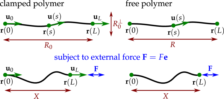
Figure 1: Wormlike chain with clamped (left) and free ends (right). Here, $\mathbf{r}(s)$ is the contour at arc length $s$, $\mathbf{u}(s)=\mathrm{d}\mathbf{r}(s)/\mathrm{d}s$ is the tangent vector of the polymer along the contour of length $L$, $\mathbf{u}_{0}=\mathbf{u}_{L}$ are the clamped ends, and $\mathbf{F}=F\mathbf{e}$ is the applied compression, $F<0$, or pulling, $F>0$, force along the fixed direction $\mathbf{e}$. Moreover, $R_{0}=\int_{0}^{L}\mathrm{d}s\ \mathbf{u}_{0}\cdot\mathbf{u}(s)$ denotes the end-to-end distance of a force-free polymer projected onto the clamped ends, $R_{0}^{\perp}=\int_{0}^{L}\mathrm{d}s\ \mathbf{u}_{0}^{\perp}\cdot\mathbf{u}(s)$ the transverse end-to-end distance, $R=|\int_{0}^{L}\mathrm{d}s\ \mathbf{u}(s)|$ the end-to-end distance of a free polymer, and $X=\int_{0}^{L}\mathrm{d}s\ \mathbf{e}\cdot\mathbf{u}(s)$ the end-to-end distance projected onto the direction of the applied force.

To elucidate the response of a semiflexible polymer to an external force $\mathbf{F}$, we account for the stretching energy,

$$\mathcal{H}_{\text{force}} =-\int_{0}^{L}\!\mathrm{d}s\ \mathbf{F}\cdot\mathbf{u}(s),$$ (3)

where the force $\mathbf{F}=F\mathbf{e}$ acts along a fixed direction $\mathbf{e}$, $|\mathbf{e}|=1$, and can be either tension, $F>0$, or compression, $F<0$. Comparing the force to the classical Euler buckling force $F_{c}$ permits to distinguish regimes of small and strong compression forces. The total energy of the system then reads

$$\frac{\mathcal{H}}{k_{\text{B}}T} =\int_{0}^{L}\!\mathrm{d}s\left[\frac{\kappa}{2k_{\text{B}}T}\left(\frac{\mathrm{d}\mathbf{u}(s)}{\mathrm{d}s}\right)^{2}-f\mathbf{e}\cdot\mathbf{u}(s)\right],$$ (4)

where we have introduced the reduced force $f=F/k_{\text{B}}T$. Since $f$ has units of an inverse length, a different choice of a dimensionless force parameter would be $fL$ or $f\ell_{\text{p}}$. The corresponding partition sum,

$$Z(\mathbf{u}_{L},L|\mathbf{u}_{0},0) =\int_{\mathbf{u}(0)=\mathbf{u}_{0}}^{\mathbf{u}(L)=\mathbf{u}_{L}}\mathcal{D}[\mathbf{u}(s)]\exp\left(-\frac{\mathcal{H}}{k_{\text{B}}T}\right),$$ (5)

can be computed by solving the associated Fokker-Planck equation Prasad et al. (2005); Kurzthaler and Franosch (2017),

$$\partial_{s}Z(\mathbf{u},s|\mathbf{u}_{0},0)=\left[f\mathbf{e}\cdot\mathbf{u}+\frac{k_{\text{B}}T}{2\kappa}\Delta_{\mathbf{u}}\right]Z(\mathbf{u},s|\mathbf{u}_{0},0),$$ (6)

with $\Delta_{\mathbf{u}}$ the angular part of the Laplacian. It is subject to the initial condition $Z(\mathbf{u},s=0|\mathbf{u}_{0},0)=\delta(\mathbf{u},\mathbf{u}_{0})$, where the $\delta$-function enforces both directions to coincide. In particular, the Fokker-Planck equation describes the evolution of the partition sum of a polymer as its arc length $s$ increases, given that the initial orientation of the polymer at $s=0$ is set by $\mathbf{u}(0)=\mathbf{u}_{0}$.

In 2D the orientation of the polymer, $\mathbf{u}=(\cos(\varphi),\sin(\varphi))^{T}$, can be parametrized in terms of the polar angle $\varphi=\angle(\mathbf{e},\mathbf{u})$, which is measured here with respect to the applied force. Thus, the Fokker-Planck equation for the partition sum $Z(\varphi,s|\varphi_{0},0)$ reads

$$\partial_{s}Z(\varphi,s|\varphi_{0},0) =\left[f\cos(\varphi)+\frac{1}{\ell_{\text{p}}}\partial_{\varphi}^{2}\right]Z(\varphi,s|\varphi_{0},0).$$ (7)

This equation is reminiscent of the Schrödinger equation of a quantum pendulum Aldrovandi and Ferreira (1980) and evaluates to an expansion in even and odd Mathieu functions, as has been elaborated for stretching forces, $f>0$, in Ref. Prasad et al. (2005) and for compression forces, $f<0$, in Ref. Kurzthaler and Franosch (2017), respectively.

In the following sections we provide a theoretical framework to obtain the probability density for the end-to-end distance projected along or transverse to the clamped ends of force-free semiflexible polymers. Furthermore, we obtain the probability density for the projected end-to-end distance of a semiflexible polymer subject to external forces. We discuss three different experimental setups encoded in the boundary conditions.

II.1 Probability density for the (projected) end-to-end distance of a force-free semiflexible polymer

We first discuss in detail the computation of the characteristic functions of clamped, cantilevered, and free semiflexible polymers, which fully characterize the probability densities of the projected end-to-end distance. We derive the corresponding probability densities by an inverse Fourier transform of the characteristic functions.

II.1.1 Clamped polymer

Here, we derive the probability density $\mathbb{P}(R_{0}|\mathbf{u}_{L},\mathbf{u}_{0})$ for the end-to-end distance projected along a fixed direction $\mathbf{e}$ of a clamped polymer, $R_{0}=\int_{0}^{L}\mathrm{d}s\ \mathbf{e}\cdot\mathbf{u}(s)$, where the initial and final orientations, $\mathbf{u}_{0}$ and $\mathbf{u}_{L}$, are considered as fixed boundary conditions. It is defined by

$$\begin{split}\mathbb{P}(R_{0}|&\mathbf{u}_{L},\mathbf{u}_{0})=\left\langle\delta\!\left(R_{0}-\int_{0}^{L}\!\mathrm{d}s\ \mathbf{e}\cdot\mathbf{u}(s)\right)\right\rangle_{0,\text{ BC}}\\ &=\frac{1}{Z_{0}}\int_{\mathbf{u}(0)=\mathbf{u}_{0}}^{\mathbf{u}(L)=\mathbf{u}_{L}}\mathcal{D}[\mathbf{u}(s)]\exp\left(-\frac{\mathcal{H}_{0}}{k_{\text{B}}T}\right)\\ &\ \ \ \ \qquad\qquad\times\delta\!\left(R_{0}-\int_{0}^{L}\!\mathrm{d}s\ \mathbf{e}\cdot\mathbf{u}(s)\right),\end{split}$$ (8)

where $\langle\cdot\rangle_{0,\text{ BC}}$ denotes the average with respect to the Boltzmann distribution with Hamiltonian $\mathcal{H}_{0}$ [Eq. (1)] and normalization $Z_{0}\equiv Z_{0}(\mathbf{u}_{L},L|\mathbf{u}_{0},0)$ [Eq. (2)] such that the ends fulfill the boundary conditions (BC) $\mathbf{u}(0)=\mathbf{u}_{0}$ and $\mathbf{u}(L)=\mathbf{u}_{L}$. To emphasize that the orientations $\mathbf{u}_{0}$ and $\mathbf{u}_{L}$ now serve as boundary conditions, rather than initial and final values as in Eqs.(6) and (7), we write the probability as conditioned with respect to the boundary conditions. The associated characteristic function for the wavevector $\mathbf{k}=k\mathbf{e}$ along the fixed direction $\mathbf{e}$ is defined as the Fourier transform,

$$\widetilde{\mathbb{P}}(k|\mathbf{u}_{L},\mathbf{u}_{0}) =\int_{-\infty}^{\infty}\!\mathrm{d}R_{0}\ \exp(-\mathsf{i}kR_{0})\mathbb{P}(R_{0}|\mathbf{u}_{L},\mathbf{u}_{0}).$$ (9)

It can be rewritten

$$\begin{split}\widetilde{\mathbb{P}}(k|\mathbf{u}_{L},\mathbf{u}_{0})&=\frac{Z_{0}(k,\mathbf{u}_{L},L|\mathbf{u}_{0},0)}{Z_{0}(\mathbf{u}_{L},L|\mathbf{u}_{0},0)}\\ &=\left\langle\exp\left[-\mathsf{i}k\int_{0}^{L}\!\mathrm{d}s\ \mathbf{e}\cdot\mathbf{u}(s)\right]\right\rangle_{0,\text{ BC}},\end{split}$$ (10)

where we have abbreviated the path integral by the partition sum for the wavenumber $k$

$$\begin{split}&Z_{0}(k,\mathbf{u}_{L},L|\mathbf{u}_{0},0)=\\ &=\int^{\mathbf{u}(L)}_{\mathbf{u}(0)}\!\mathcal{D}\left[\mathbf{u}(s)\right]\exp\left[-\left(\frac{\mathcal{H}_{0}}{k_{\text{B}}T}+\mathsf{i}k\int_{0}^{L}\!\mathrm{d}s\ \mathbf{e}\cdot\mathbf{u}(s)\right)\right].\end{split}$$ (11)

The path integral differs from the partition sum of a polymer subject to an external force, $Z(\mathbf{u}_{L},L|\mathbf{u}_{0},0)$ [Eq. (5)], only by allowing the force to become formally complex. Therefore, the Fokker-Planck equation associated with the path integral assumes the same form, via the mapping $f\mapsto-\mathsf{i}k$,

$$\partial_{s} Z_{0}(k,\varphi,s|\varphi_{0},0)=$$

$$=\left(-\mathsf{i}k\cos(\varphi)+\frac{1}{\ell_{\text{p}}}\partial^{2}_{\varphi}\right)Z_{0}(k,\varphi,s|\varphi_{0},0).$$ (12)

Here, we have employed again the polar angle $\varphi=\angle(\mathbf{e},\mathbf{u})$ between the direction $\mathbf{e}$ and the tangent vector $\mathbf{u}$. Thus, the equation can again be solved using an expansion in appropriate angular eigenfunctions $z(\varphi)$. Inserting the separation ansatz $\exp(-\lambda s)z(\varphi)$ into Eq. (12) we obtain the eigenvalue problem

$$\left[\lambda-\mathsf{i}k\cos(\varphi)+\frac{1}{\ell_{\text{p}}}\frac{\mathrm{d}^{2}}{\mathrm{d}\varphi^{2}}\right]z(\varphi) =0.$$ (13)

A change of variables, $x=\varphi/2$, and rearranging terms leads to the well-known Mathieu equation DLMF ; Olver et al. (2010)

$$\left[\frac{\mathrm{d}^{2}}{\mathrm{d}x^{2}}+(a-2q\cos(2x))\right]z(x) =0,$$ (14)

with (yet imaginary) deformation parameter $q=2\mathsf{i}k\ell_{\text{p}}$ and eigenvalue $a=4\ell_{\text{p}}\lambda$.

The general solution of Eq. (12) is then expressed as a linear combination of $\pi$-periodic even and odd Mathieu functions, $\text{ce}_{2n}(q,x)$ and $\text{se}_{2n+2}(q,x)$, with associated eigenvalues $a_{2n}(q)=4\ell_{\text{p}}\lambda_{n}$ and $b_{2n+2}(q)=4\ell_{\text{p}}\lambda_{n}$ DLMF ; Olver et al. (2010), respectively. The Mathieu functions constitute a complete, orthogonal, and normalized set of eigenfunctions, $\int_{0}^{2\pi}\!\mathrm{d}x\ \text{ce}_{2n}(q,x)\text{ce}_{2m}(q,x)=\delta_{nm}\pi$, and similarly for $\text{se}_{2n+2}(q,x)$ Ziener et al. (2012). As the Mathieu functions are periodic, they can be expressed as deformed cosines and sines:

$$\text{ce}_{2n}(q,x) =\sum_{m=0}^{\infty}A_{2m}^{2n}(q)\cos(2mx),$$ (15)

$$\text{se}_{2n+2}(q,x) =\sum_{m=0}^{\infty}B_{2m+2}^{2n+2}(q)\sin[(2m+2)x],$$ (16)

where the Fourier coefficients, $A_{2m}^{2n}(q)$ and $B_{2m+2}^{2n+2}(q)$, are fully determined by the recurrence relations [Eqs. (26)- (27) in the appendix A].

Hence, the full solution for the partition sum in terms of the eigenfunctions reads

$$\begin{split}&Z_{0}(k,\varphi_{L},L|\varphi_{0},0)=\\ &=\frac{1}{2\pi}\sum_{n=0}^{\infty}\bigl{[}\text{ce}_{2n}(q,\varphi_{0}/2)\text{ce}_{2n}(q,\varphi_{L}/2)e^{-a_{2n}(q)L/4\ell_{\text{p}}}\\ &\ \ \ \ +\text{se}_{2n+2}(q,\varphi_{0}/2)\text{se}_{2n+2}(q,\varphi_{L}/2)e^{-b_{2n+2}(q)L/4\ell_{\text{p}}}\bigr{]}.\end{split}$$ (17)

In particular, if $\varphi_{0}=0$ ($\varphi_{0}=\pi/2$ ) the wavevector is parallel (perpendicular) to the initial orientation of the polymer. Thus, our solution permits to recover the probability density for the end-to-end distance of the polymer projected along the clamped ends or in any other direction. The cases for clamped polymers follow by setting $\varphi_{L}=\varphi_{0}$.

Interestingly, the conformations of the semiflexible polymer can be regarded as the trajectory of a self-propelled particle, which suggests that the methodology of both systems is intimately related to one another. In particular, exact solutions for the partition sum of a semiflexible polymer [Eq. (17)] can be directly mapped to the characteristic function of the displacements of an active Brownian particle Kurzthaler et al. (2016); Kurzthaler and Franosch (2017); Kurzthaler et al. (2017). Thus, as for the mathematical analog of the self-propelled agent, the eigenvalue problem [Eq. (14)] is non-hermitian and, therefore, the Mathieu functions and the corresponding eigenvalues assume complex values Ziener et al. (2012). The characteristic function of a clamped polymer becomes complex, and although it is formally the same as the partition sum of a polymer subject to an external force [Eq. (5)] Kurzthaler and Franosch (2017), it exhibits a qualitatively different behavior. For details on the numerical evaluation of the eigenfunctions and eigenvalues we refer to appendix A.

The probability density for the projected end-to-end distance of a clamped polymer is obtained by an inverse Fourier transform of the characteristic function,

$$\mathbb{P}(R_{0}|\mathbf{u}_{L},\mathbf{u}_{0}) =\int_{-\infty}^{\infty}\!\frac{\mathrm{d}k}{2\pi}\ \exp(\mathsf{i}kR_{0})\widetilde{\mathbb{P}}(k|\mathbf{u}_{L},\mathbf{u}_{0}),$$ (18)

which we evaluate numerically using the Filon trapezoidal scheme Tuck (1967).

II.1.2 Cantilevered polymer

The probability density of a cantilevered polymer, $\mathbb{P}(R_{0}|\mathbf{u}_{0})$, can be obtained by marginalizing the probability density of a clamped polymer, $\mathbb{P}(R_{0}|\mathbf{u}_{L},\mathbf{u}_{0})$, i.e. integrating over the final orientations, $\mathbb{P}(R_{0}|\mathbf{u}_{0})=\int\!\mathrm{d}\mathbf{u}_{L}\ \mathbb{P}(R_{0}|\mathbf{u}_{L},\mathbf{u}_{0})\mathbb{P}(\mathbf{u}_{L}|\mathbf{u}_{0})$. The probability density that a polymer has a final orientation $\mathbf{u}_{L}$ given the initial orientation $\mathbf{u}_{0}$, reads $\mathbb{P}(\mathbf{u}_{L}|\mathbf{u}_{0})=Z_{0}(\mathbf{u}_{L},L|\mathbf{u}_{0},0)/Z_{0}(L|\mathbf{u}_{0},0)$, where the normalization evaluates to one, $Z_{0}(L|\mathbf{u}_{0},0)=\int\!\mathrm{d}\mathbf{u}_{L}\ Z_{0}(\mathbf{u}_{L},L|\mathbf{u}_{0},0)=1$. Then the corresponding characteristic function can be calculated by

$$\begin{split}\widetilde{\mathbb{P}}(k|\mathbf{u}_{0})&=Z_{0}(L|\varphi_{0},0)^{-1}\int_{0}^{2\pi}\!\mathrm{d}\varphi_{L}\ Z_{0}(k,\varphi_{L},L|\varphi_{0},0)\\ &=\sum_{n=0}^{\infty}A_{0}^{2n}(q)\text{ce}_{2n}(q,\varphi_{0}/2)\exp\left[-a_{2n}(q)L/4\ell_{\text{p}}\right],\end{split}$$ (19)

where we have integrated Eq. (17) over the final orientations $\varphi_{L}$. Here, $A_{0}^{2n}(q)$ are the Fourier coefficients of the even Mathieu functions [Eq. (15)], while the odd Mathieu functions do not contribute anymore. As for a clamped polymer, the probability density $\mathbb{P}(R_{0}|\mathbf{u}_{0})$ can be obtained numerically by an inverse Fourier transform Tuck (1967) of $\widetilde{\mathbb{P}}(k|\mathbf{u}_{0})$.

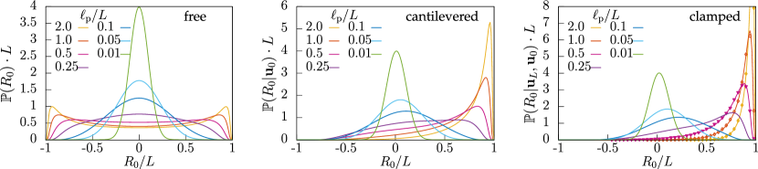
Figure 2: Probability density for the end-to-end distance $R_{0}$ of a semiflexible polymer with free, $\mathbb{P}(R_{0})$ (left panel), cantilevered, $\mathbb{P}(R_{0}|\mathbf{u}_{0})$ (middle panel), and clamped ends, $\mathbb{P}(R_{0}|\mathbf{u}_{L},\mathbf{u}_{0})$ (right panel), projected onto the direction $\mathbf{e}$. For cantilevered and clamped polymers $\mathbf{e}$ is parallel to the initial (and final) orientation $\mathbf{u}_{0}$($=\mathbf{u}_{L}$), respectively. Here, $L$ denotes the contour length and $\ell_{\text{p}}$ the persistence length of the polymer. Selected pseudo-dynamic simulations are indicated by symbols.

II.1.3 Free polymer

The probability density, $\mathbb{P}(R_{0})$, for the projected end-to-end distance $R_{0}$ of a free polymer is obtained by integrating the probability density of a clamped polymer over the final and initial orientations, $\mathbb{P}(R_{0})=\int\!\mathrm{d}\mathbf{u}_{0}\int\!\mathrm{d}\mathbf{u}_{L}\ \mathbb{P}(R_{0}|\mathbf{u}_{L},\mathbf{u}_{0})\mathbb{P}(\mathbf{u}_{L}|\mathbf{u}_{0})\mathbb{P}(\mathbf{u}_{0})$, where the probability for the initial orientation is $\mathbb{P}(\mathbf{u}_{0})=Z_{0}(L|\mathbf{u}_{0},0)/Z_{0}(L)$ with normalization $Z_{0}(L)=\int\!\mathrm{d}\mathbf{u}_{0}\ Z_{0}(L|\mathbf{u}_{0},0)=2\pi$. Then the Fourier transform evaluates to

$$\begin{split}\widetilde{\mathbb{P}}(k)&=\frac{1}{Z_{0}(L)}\int_{0}^{2\pi}\!\mathrm{d}\varphi_{0}\int_{0}^{2\pi}\!\mathrm{d}\varphi_{L}\ Z_{0}(k,\varphi_{L},L|\varphi_{0},0)\\ &=\sum_{n=0}^{\infty}\left[A_{0}^{2n}(q)\right]^{2}\exp\left[-a_{2n}(q)L/4\ell_{\text{p}}\right].\end{split}$$ (20)

As for clamped and cantilevered polymers, the probability density $\mathbb{P}(R_{0})$ for the projected end-to-end distance $R_{0}$ can be calculated numerically by an inverse Fourier transform Tuck (1967) of $\widetilde{\mathbb{P}}(k)$.

In addition to the probability density for the projected end-to-end distance, our method permits to obtain an exact solution for the probability density, $\mathbb{P}(R)$, of the end-to-end distance, $R=|\mathbf{R}|=|\int_{0}^{L}\!\mathrm{d}s\ \mathbf{u}(s)|$, of a free polymer. The probability density for the end-to-end distance $R$ of a free polymer is circularly symmetric and therefore the associated characteristic function depends only on the magnitude of the wavevector $k=|\mathbf{k}|$. Thus, after averaging over the directions of $\mathbf{k}$, we obtain the probability density by an inverse Hankel transform of the characteristic function $\widetilde{\mathbb{P}}(k)$ [Eq. (20)] via

$$\mathbb{P}(R) =\int_{0}^{\infty}\!\frac{\mathrm{d}k}{2\pi}\ kJ_{0}(kR)\widetilde{\mathbb{P}}(k),$$ (21)

where $J_{0}(\cdot)$ denotes the Bessel function of order zero. For the numerical evaluation we employ a Filon trapezoidal scheme Barakat and Sandler (2000).

II.2 Probability density for the end-to-end distance projected onto the applied force

To include an external force into the theory developed in the previous section, in principle, we only have to replace the Hamiltonian $\mathcal{H}_{0}$ [Eq. (1)] by $\mathcal{H}=\mathcal{H}_{0}+\mathcal{H}_{\text{force}}$ [Eq. (4)], and adjust all quantities, such as the normalization $Z_{0}(\mathbf{u}_{L},L|\mathbf{u}_{0})$ and the path integral $Z_{0}(k,\mathbf{u}_{L},L|\mathbf{u}_{0})$, accordingly. Here, we restrict our discussion to forces $\mathbf{F}=F\mathbf{e}$ that are (anti-) parallel to the wave vector ($\mathbf{k}=k\mathbf{e}$), depending on whether a compressive, $F<0$, or pulling force, $F>0$, is applied.

The solution strategy for the probability density,

$$\mathbb{P}(X|\text{BC}) =\left\langle\delta\!\left(X-\int_{0}^{L}\!\mathrm{d}s\ \mathbf{e}\cdot\mathbf{u}(s)\right)\right\rangle_{\text{BC}},$$ (22)

remains the same as for the force-free distribution. Note, that $X$ is always measured as end-to-end distance projected onto the fixed direction $\mathbf{e}$. In fact, for clamped and cantilevered polymers it corresponds to the end-to-end distance projected onto the direction of the applied force, whereas for free polymers the end-to-end distance $X$ is measured in one specific direction $\mathbf{e}$ of the circularly symmetric probability density.

In principle, one can also derive the probability density by reweighting the force-free probability density for the (projected) end-to-end distance $R$ ($R_{0}$) with the Boltzman factor for the force bias, e.g. for clamped ends: $\mathbb{P}(X|\mathbf{u}_{L},\mathbf{u}_{0})\propto\exp(FX/k_{\text{B}}T)\mathbb{P}(R_{0}=X|\mathbf{u}_{L},\mathbf{u}_{0})$. Yet, the numerical evaluation becomes unstable for compression forces in the vicinity of the critical Euler buckling force, where the Boltzman factor exponentially inflates small round-off and truncation errors in the numerical evaluation of the infinite sums [Eqs. (17), (19), (20)]. Therefore, we rely on exact solutions for the corresponding characteristic functions.

The partition sums for clamped, $Z(\varphi_{L},L|\varphi_{0},0)$, cantilevered, $Z(L|\varphi_{0},0)$, and free polymers, $Z(L)$, subject to external forces have been computed in Refs. Prasad et al. (2005); Kurzthaler and Franosch (2017). These are now used to normalize the characteristic functions (instead of $Z_{0}$). To compute the path integral for the wave vector, $\mathbf{k}=k\mathbf{e}$, of a polymer subject to an external force,

$$\begin{split}&Z(k,\varphi_{L},L|\varphi_{0},0)=\\ &=\int^{\mathbf{u}(L)}_{\mathbf{u}(0)}\!\mathcal{D}\left[\mathbf{u}(s)\right]\exp\left[-\left(\frac{\mathcal{H}_{0}}{k_{\text{B}}T}+\left(\mathsf{i}k-f\right)\int_{0}^{L}\!\mathrm{d}s\ \mathbf{e}\cdot\mathbf{u}(s)\right)\right],\end{split}$$ (23)

we solve the associated Fokker-Planck equation,

$$\partial_{s} Z(k,\varphi,L|\varphi_{0},0)=$$

$$=\left[\left(f-\mathsf{i}k\right)\cos(\varphi)+\frac{1}{\ell_{\text{p}}}\partial^{2}_{\varphi}\right]Z(k,\varphi,L|\varphi_{0},0),$$ (24)

where $\varphi=\angle(\mathbf{e},\mathbf{u})$ is the angle between the direction $\mathbf{e}$ of the force/wavevector and the orientation $\mathbf{u}$, and $f=F/k_{\text{B}}T$ denotes the reduced force with units of an inverse length. For compression forces, $f=-|f|$, the Fokker-Planck equation assumes the form of Eq. (12) with corresponding solution [Eq. (17)], yet, with a different complex deformation parameter

$$q=2\ell_{\text{p}}\left(|f|+\mathsf{i}k\right).$$ (25)

Similarly, the characteristic functions for cantilevered and free polymers can be transferred from Eq. (19) and from Eq. (20), respectively. Interestingly, for pulling forces, $f=|f|$, a change of variables, $\varphi_{0}\mapsto\pi-\varphi_{0}$ and $\varphi_{L}\mapsto\pi-\varphi_{L}$, in Eqs. (19) and (17), and $q=2\ell_{\text{p}}\left(|f|-\mathsf{i}k\right)$ yields the corresponding characteristic functions for cantilevered and clamped polymers, respectively. For free polymers, the solution remains identical to that of a compressive force [Eq. (20)].

The probability densities for the end-to-end distance $X$ [Eq. (22)] of a clamped, $\mathbb{P}(X|\varphi_{L},\varphi_{0})$, cantilevered, $\mathbb{P}(X|\varphi_{0})$, and free polymer, $\mathbb{P}(X)$, are obtained by a numerical inverse Fourier transform of the corresponding characteristic functions Tuck (1967).

III Results – force-free behavior

To explore the response of a single semiflexible polymer to external forces, a full characterization of the force-free polymer behavior serves as a reference. We elucidate the force-free behavior of a wormlike chain with clamped and cantilevered in terms of the probability densities for the projected end-to-end distance, as the clamping introduces a characteristic direction to the system. Here, we focus on the projection along and perpendicular to the clamped ends. We compare these results with the probability density for the projected end-to-end distance of a free polymer and we also discuss the probability density for the end-to-end distance of a free polymer, as has been elaborated earlier Samuel and Sinha (2002); Mehraeen et al. (2008). Exemplarily, we have corroborated selected exact predictions for the probability densities with pseudo-dynamic simulations elaborated in Ref. Kurzthaler and Franosch (2017) (see appendix B for simulation details).

III.1 Projected end-to-end distance (along clamped ends)

Clamped ends naturally introduce a characteristic direction to the configurations of the polymers and, in contrast to the circularly symmetric probability density of a free polymer (see Fig. 2 (left panel)), their probability densities projected along the clamped ends are asymmetric (see Fig. 2 (middle panel) for cantilevered and Fig. 2 (right panel) for clamped polymers). In particular, the asymmetry indicates that the configurations aligned along the opposite direction than the initial (and final) orientations of the polymer remain less likely than the alignment along the clamped ends. This effect becomes most pronounced for stiff polymers, where the most favorable end-to-end distance is almost their contour length, $R_{0}/L=1$.

However, the probability densities for the projected end-to-end distance reveal very similar behavior for clamped and cantilevered polymers. They exhibit a left-skewed form, i.e. the left tail of the distribution is longer. The peak decreases and the probability density broadens for decreasing stiffness due to thermal fluctuations. For more flexible polymers an alignment into the opposite direction of the clamped ends becomes more probable as the boundary conditions are less restrictive, and, in particular, for flexible polymers, $\ell_{\text{p}}/L\ll 1$, we find a Gaussian distribution located at zero end-to-end distance, which narrows for increasing flexibility.

III.2 End-to-end distance of a free polymer

The circularly symmetric end-to-end probability density of a free polymer displays peculiar behavior with respect to the persistence length, see Fig. 3.

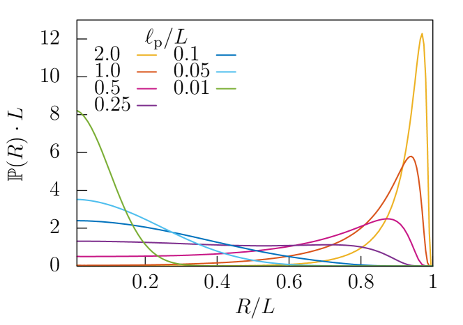
Figure 3: Probability density $\mathbb{P}(R)$ for the end-to-end distance $R$ of a semiflexible polymer with free ends. Here, $L$ denotes the contour length and $\ell_{\text{p}}$ the persistence length of the polymer.

For stiff polymers, the distribution exhibits a peak located in the vicinity of a fully stretched configuration, $R/L=1$. Increasing the flexibility, shifts the peak away, and a second peak, positioned close to zero, evolves at the transition between rather stiff and flexible polymers. In particular, in the regime of $\ell_{\text{p}}/L\in[0.24,0.35]$ the distribution displays a bimodal shape, which is hardly visible in the figure due to scaling. For flexible polymers, $\ell_{\text{p}}/L\ll 1$, the peak approaches zero end-to-end distance, as anticipated by the Gaussian chain. Here, the distribution becomes more narrow for more flexible polymers. As expected, these findings are in agreement with earlier results obtained in Refs. Samuel and Sinha (2002); Mehraeen et al. (2008).

III.3 End-to-end distance transverse to the clamped ends

Transverse fluctuations of the free end of a cantilevered polymer are quantified in terms of the probability density for the end-to-end distance projected perpendicular to the clamped end $R_{0}^{\perp}$, see Fig. 4 (top panel). The probability densities for polymers with different bending rigidities display an interesting reentrant behavior, such that for flexible, $\ell_{\text{p}}/L\ll 1$, and for stiff polymers, $\ell_{\text{p}}/L\gg 1$, the probability density exhibits a single peak centered at zero projected end-to-end distance, $R_{0}^{\perp}/L=0$. Thus, the free end of a stiff cantilevered polymer prefers to align along the same direction as the clamped end.

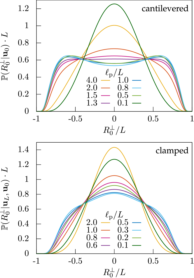
Figure 4: Probability density for the end-to-end distance $R_{0}^{\perp}$ of a semiflexible polymer with cantilevered, $\mathbb{P}(R_{0}^{\perp}|\mathbf{u}_{0})$ (top panel), and clamped ends, $\mathbb{P}(R_{0}^{\perp}|\mathbf{u}_{L},\mathbf{u}_{0})$ (bottom panel), projected onto the transverse direction of the initial (and final) orientation $\mathbf{u}_{0}$($=\mathbf{u}_{L}$).

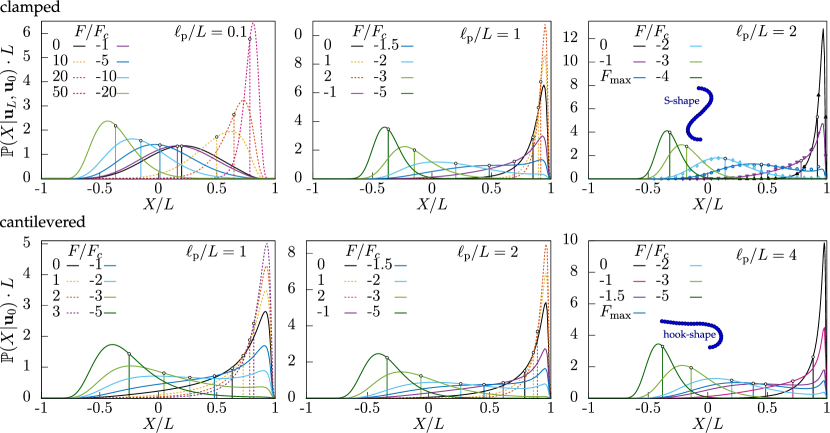
Figure 5: Probability density of semiflexible polymers with clamped ends $\mathbf{u}_{0}=\mathbf{u}_{L}$, $\mathbb{P}(X|\mathbf{u}_{L},\mathbf{u}_{0})$ (top row), and cantilevered ends, $\mathbb{P}(X|\mathbf{u}_{0})$ (bottom row), for the end-to-end distance $X$ projected along the applied force, $\mathbf{F}=F\mathbf{u}_{0}$. Figures show semiflexible polymers of different persistence lengths $\ell_{\text{p}}$ subject to external pulling (dashed lines) and compression (solid lines) forces $F$. Here, $L$ denotes the contour length of the polymer, $F_{c}=\pi^{2}\kappa/(\gamma L)^{2}$ is the critical Euler buckling force with $\gamma=1$ for clamped and $\gamma=2$ for cantilevered polymers, and $F_{\text{max}}$ is the force at maximal susceptibility $\chi$. Vertical lines with circles indicate the projected mean end-to-end distance $\langle X\rangle/L$ extracted from the force-extension relations Kurzthaler and Franosch (2017). Selected pseudo-dynamic simulations are indicated by symbols.

In the case of a flexible polymer, the boundary conditions can be neglected and the probability densities for the end-to-end distance of a free polymer follow a Gaussian [Sec. III.2]. As an intriguing fingerprint of the semiflexibility of the polymer, $\ell_{\text{p}}/L\simeq 1$, the probability density is characterized by a bimodal shape indicating the transverse fluctuations of the free end with respect to the clamped end. This peculiar behavior arising in semiflexible polymers has already been observed earlier for polymers in 2D in terms of computer simulations Lattanzi et al. (2004) and an approximate theory Benetatos et al. (2005). Similar behavior has been observed in the distribution function of a cantilevered polymer in 3D, which has been elaborated formally exactly in Fourier-Laplace space by an expansion in Legendre polynomials Semeriyanov and Stepanow (2007).

Qualitatively different behavior is observed for the transverse fluctuations of a polymer with two clamped ends [Fig. 4 (bottom panel)]. Here, the probability densities display a prominent peak at zero transverse end-to-end distance, $R_{0}^{\perp}/L=0$, for all bending rigidities $\ell_{\text{p}}/L$. Yet, in the regime of semiflexible polymers, $\ell_{\text{p}}/L\simeq 1$, the probability densities additionally exhibit two heavy tails, reflecting the transverse fluctuations between the clamped ends.

IV Results – semiflexible polymer subject to external loads

In striking contrast to the buckling behavior of a classical rigid rod, which does not yield at all but starts to buckle at the critical Euler buckling force, thermal fluctuations smear out the Euler buckling instability for semiflexible polymers Kurzthaler and Franosch (2017). Yet, a peak in the susceptibility of a semiflexible polymer is still observed close to the critical Euler buckling force and, thus, we refer to this behavior as the buckling transition of a semiflexible polymer. In particular, the smearing of the Euler buckling instability results in a rapidly decaying force-exension relation with a broad variance at the buckling transition, which is reminiscent of a smeared discontinuous phase transition in a finite system. Moreover, these lowest-order moments indicate a non-Gaussian probability density of the polymer at the bucking transition and, therefore, a profound analysis of the full probability density is required to adequately interpret these findings.

Here, we analyze the response of semiflexible polymers to external forces in terms of the probability densities for their projected end-to-end distance, which permit to shed light on the polymer configurations in the presence of a compression or elongation force. In particular, we discuss polymers with different bending rigidities and boundary conditions, see Fig. 5 for clamped and cantilevered polymers and Fig. 6 for free polymers.

IV.1 Clamped and cantilevered polymers

As predicted from the force-free behavior of clamped and cantilevered polymers, the probability density for the end-to-end distance of stiff polymers displays a left-skewed peak close to a fully stretched configuration, $X/L=1$, whereas more flexible polymers have a broad probability density which approaches a Gaussian for large flexibility. Under extensional forces these polymers approach almost their full contour length with increasing forces, yet, stronger forces are required to elongate more flexible polymers, than stiffer polymers, see Fig. 5 dashed lines. For increasing forces the probability densities shift towards full extension $X/L=1$, where they narrow significantly. The mean end-to-end distance projected onto the direction of the applied force $\langle X\rangle/L$ can be obtained by directly averaging the probability distribution or from the previously calculated exact force-extentsion relation Kurzthaler and Franosch (2017). We have checked that both approaches yield the same result corroborating our methods. Fig. 5 reveals that the most probable configuration is even longer than the mean end-to-end distance, however, the heavy tail of the distribution also allows for more coil-like structured configurations due to thermal fluctuations. Similar behaviors are observed for clamped and cantilevered polymers, respectively.

Although the stretching behavior of these clamped and cantilevered polymers remains similar with respect to their stiffness, flexible polymers do not display a buckling transition anymore. For flexible polymers, the probability density assumes a unimodal shape for all applied forces; however, the peak of the probability density shifts towards negative end-to-end distances in the presence of compression forces, where the probability density assumes a right-skewed form that sharpens with increasing forces [Fig. 5 (left panel, top)].

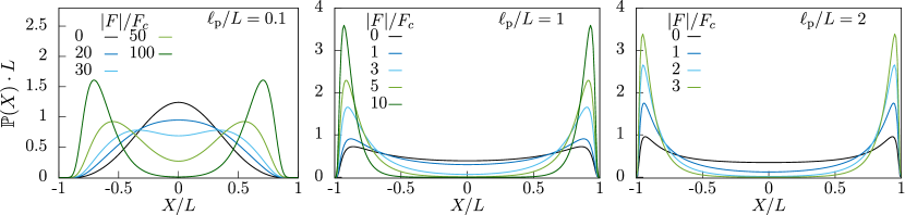
Figure 6: Intersection of the circularly symmetric probability density $\mathbb{P}(X)$ for the end-to-end distance $X$ of semiflexible polymers with free ends and different persistence lengths $\ell_{\text{p}}$ subject to external forces $|F|$. Here, $L$ denotes the contour length of the polymer and the critical Euler buckling force $F_{c}=\pi^{2}\kappa/(\gamma L)^{2}$ with $\gamma=2$ is used to normalize the forces.

In striking contrast, stiffer polymers display a bimodal distribution at forces in the vicinity of the critical force $F_{\text{max}}$, where the susceptibility, $\chi=\left(\partial\langle X\rangle/\partial F\right)_{T}$, defined as the derivative of the mean end-to-end distance $\langle X\rangle$ with respect to the applied force $F$, exhibits a maximum; compare, for example, Fig. 2 (d) in Ref. Kurzthaler and Franosch (2017) and Fig. 5 (right panel, top). The bimodal distribution reflects two favored configurations for clamped and cantilevered polymers under compression. One configuration constitutes an almost elongated configuration, which resists the applied compression force, and the second configuration reflects the bending of the polymer as response to the compression. In the buckled state, clamped polymers exhibit an S-shaped configuration with both ends aligned against the applied force (see inset in Fig. 5 (right panel, top)). Similarly, cantilevered polymers assume a hook-shaped configuration with the free end aligned along the applied force (see inset in Fig. 5 (right panel, bottom)). The corresponding mean end-to-end distance $\langle X\rangle/L$ Kurzthaler and Franosch (2017) is located between the two peaks and, thus, does not reflect the favored configuration of the polymer. Moreover, these two modes become more prominent for polymers of increasing stiffness, which allows for a restricted number of chain configurations only, whereas they are smeared out for more flexible polymers due to thermal fluctuations. For larger forces, the S-shaped (for clamped) and the hook-shaped (for cantilevered) configurations take over and the probability density exhibits a single peak located at a negative end-to-end distance. Interestingly, a bimodal shape is also observed in the probability density for the order parameter of a finite system at a smeared discontinuous phase transition Binder and Heermann (1992). In particular, the probability density dispays two peaks at the transition temperature, whereas one mode disappears upon in/decreasing the temperature.

We have validated our analytical results by comparing the mean projected end-to-end distance $\langle X\rangle$ and the standard deviation $\langle(X-\langle X\rangle)^{2}\rangle$ obtained numerically from the probability distribution to the force extension relation and the susceptibility $\chi=\langle(X-\langle X\rangle)^{2}\rangle/k_{\text{B}}T$ elaborated exactly in Ref. Kurzthaler and Franosch (2017). In addition, we have corroborated the exact probability densities for selected parameter sets with pseudo-dynamic simulations indicated by symbols in Fig.5 (see appendix B for simulation details).

IV.2 Free polymer

The behavior of free polymers under stretching and compression is identical, as the ends are free to align into the direction of the applied force. In particular, by integrating over the initial orientations the corresponding probability densities of the end-to-end distance become circularly symmetric, and therefore, it suffices to consider a projection along a specific direction only. For rather stiff force-free polymers we find a probability density with two peaks located in the vicinity of $X/L=\pm 1$, which become larger for increasing stiffness, see Fig. 6 for $\ell_{\text{p}}/L=1,2$. Note, that the negative end-to-end distance corresponds to polymers aligned along the opposite direction than the projection vector. Applying an external force ((anti-) parallel to the projection vector), the distributions become more narrow and the modes approach the fully elongated configuration. In the case of more flexible polymers the two peaks in the force-free distribution vanish and the probability density displays only a single peak at $X=0$ [Fig. 6, $\ell_{\text{p}}/L=0.1$]. In the presence of an external force two peaks emerge and approach the vicinity of $X/L=\pm 1$ for increasing forces. Here, the forces required to fully stretch the polymer are much larger than for stiffer polymers. Thus, as for clamped and cantilevered polymers, thermal fluctuations allow flexible polymers to resist more strongly, than stiffer polymers, which is reflected in broader distributions.

V Summary and conclusion

We have derived exact solutions for the probability densities for the (projected) end-to-end distance of a wormlike chain in the presence of external forces and compared them to the force-free case. Our analytic results have permitted to elucidate the stretching behavior and the buckling transition of semiflexible polymers with arbitrary bending rigidities for different experimental setups. As most prominent feature we have found a bimodal probability density for the projected end-to-end distance in the vicinity of the buckling transtion, which reflects the stretched and S- (or hook-) shaped configurations of clamped (or cantilevered) polymers induced by the compression. In particular, we have observed a passage from a unimodal distribution at small forces reflecting the stretched configuration of the polymer, to a bimodal distribution at the buckling transition, and again to a unimodal distribution for the S- (or hook-) shaped configuration at large forces. Interestingly, this behavior is reminiscent of a discontinuous phase transition in a finite system, where the probability density for the order parameter exhibits two modes close to the transition temperature, which reduce to one upon in/decrasing temperatures Binder and Heermann (1992). In this sense, increasing the stiffness and thereby suppressing the thermal fluctuations of the semiflexible polymer, plays the same role as the infinite volume limit close to a discontinuous phase transition. Moreover, the large variance of the force-extension relation at the buckling transition Kurzthaler and Franosch (2017) serves to a large extend as a measure for the distance between the two favored configurations, in contrast to the width of a unimodal distribution. Hence, the full probability density has provided essential information for the correct interpretation of these low-order moments, as is fundamental to understand non-Gaussian behavior.

However, these features are only present in the case of semiflexible polymers $\ell_{\text{p}}/L\simeq 1$, whereas flexible polymers $\ell_{\text{p}}/L\ll 1$ respond qualitatively differently to external forces. In particular, the probability densities for flexible polymers display only one mode independent of the applied force, which becomes broader for increasing flexibility. Thus, flexible polymers can resist external forces more effectively due to the presence of strong thermal fluctuations.

Force spectroscopy techniques have already been applied successfully to elucidate the nonlinear elastic response of a variety of biopolymers in terms of force-extension relations. In these experiments, one end of the polymer is usually tethered to a surface and a colloidal bead is attached to the other end, which reflects the setup of a cantilevered polymer. Using, for example, magneticGosse and Croquette (2002) or optical tweezers Mehta et al. (1999) the colloid can be trapped, moved and steered, thereby, exerting a force on the attached polymer. Although experimental observations are mostly restricted to pulling forces, also compression forces could be applied in a similar manner. Moreover, tracking the bead should in principle permit to extract reliable information on the probability density for the end-to-end distance of the polymer. Thus, we anticipate, that a direct comparison of experiments to our theoretical predictions allows deepening the understanding of the elastic behavior of semiflexible polymers in the presence of external forces.

Further theoretical investigations are needed to unravel the elastic properties of different types of polymers, including, for instance polymers in 3D or curved polymers. Our solution strategy can be transferred to semiflexible polymers in 3D, where the Mathieu functions are replaced by the generalized spheroidal wave functions, as elaborated for the mathematical analog of an active Brownian particle in bulk Kurzthaler et al. (2016). Similarly, analytical progress can be achieved by accounting for a spotaneous curvature of the polymer configuration such that the classical reference system displays a circular arc Potemkin et al. (2004). In this case the mathematical analog is the Brownian circle swimmer and the eigenfunctions become generalizations of Mathieu functions Kurzthaler and Franosch (2017).

In contrast to an external force acting on the end of the polymer, external fields, including, for examlpe, hydrodynamic flows Perkins et al. (1995); Larson et al. (1997); Smith and Chu (1998) or electric fields Ferree and Blanch (2003); Li et al. (2012), can be used for the manipulation of single polymers. Theoretical progress Lamura et al. (2001); Benetatos and Frey (2004); Manca et al. (2012) has been made by considering a tethered polymer in an external field, where a force acts on each bead of the discretized polymer chain. Similar to the behavior of a polymer under extension, the tethered polymer aligns along the direction of the external field and its mean configuration is characterized by the orientation of the final segment and its presistence length Lamura et al. (2001). In the presence of an additional external force applied opposite to the direction of the external field, the polymer displays a hook-shaped configuration Manca et al. (2012), analogous to a cantilevered polymer under compression. Interestingly, charged polymers display even more complex behavior in an electric field, as the charge distribution determines the direction of the polymer deformations Benetatos and Frey (2004). In particular, an electric field can also compress the polymer and the elastic behavior should be qualitatively similar to the buckling transition of a wormlike chain.

In addition to the elastic properties of single polymers, the behavior of single polymers inside cells and the buckling behavior of entire networks composed of semiflexible polymers remains to be fully understood. We anticipate, that the single-polymer behavior in free space, as elaborated here, constitutes the reference for the more realistic case of polymers immersed in a densely crowded environment Keshavarz et al. (2016); Leitmann et al. (2016); Schöbl et al. (2014) and moreover, serves as input for the analysis of polymer networks Amuasi et al. (2015); Broedersz and MacKintosh (2014); Carrillo et al. (2013); Chaudhuri et al. (2007); Claessens et al. (2006); Huisman et al. (2008); Kroy and Frey (1996); MacKintosh et al. (1995); Plagge et al. (2016); Razbin et al. (2015); Storm et al. (2005). In a simplified description, these polymeric networks can be regarded as entangled solutions of semiflexible polymers, which can cross or loop each other, exhibit branching points, or are tightly connected by cross-links. Consequently, a polymer naturally experiences compression or stretching forces due to the constraints set by the surrounding environment. Thus, our predictions for the conformational properties of single polymers induced by external forces may constitute a convenient starting point for studying the equilibrium properties of polymer networks.

Beyond the force-free behavior of networks, the elastic response of these polymeric structures to external loads is of fundamental interest and is substantially governed by the buckling behavior and the corresponding shapes of the single components. In particular, our theoretical predictions for the probability densities of semiflexible polymers of arbitrary stiffness may be useful to explore the mechanical stability of such networks in the regime of strong compression, where the polymers display strongly pronounced S- or hook-shaped configurations and the weakly-bending approximation breaks down.

Appendix

Appendix A Numerical evaluation of the Mathieu functions

The even and odd Mathieu functions, $\text{ce}_{2n}(q)$ [Eq. (15)] and $\text{se}_{2n+2}(q)$ [Eq. (16)], and the associated eigenvalues, $a_{2n}(q)$ and $b_{2n+2}(q)$, are evaluated numerically by solving the recurrence relations for the Fourier coefficients DLMF ; Olver et al. (2010); Ziener et al. (2012). In particular, we obtain the recurrence relations for the Fourier coefficients of the even Mathieu functions $A_{2m}^{2n}(q)$ by inserting Eq. (15) into the Mathieu equation [Eq. (14)],

$$\begin{split}a_{2n}A_{0}^{2n}-qA_{2}^{2n}&=0,\\ (a_{2n}-4)A_{2}^{2n}-q(2A_{0}^{2n}+A_{4}^{2n})&=0,\\ (a_{2n}-4m^{2})A_{2m}^{2n}-q(A_{2m-2}^{2n}+A_{2m+2}^{2n})&=0,\quad m\geq 2,\end{split}$$ (26)

and, similarly, for the Fourier coefficients of the odd Mathieu functions $B_{2m+2}^{2n+2}(q)$

$$\begin{split}(b_{2n+2}-4)B_{2}^{2n+2}-qB_{4}^{2n+2}&=0,\\ (b_{2n+2}-4m^{2})B_{2m}^{2n+2}-q(B_{2m-2}^{2n+2}+B_{2m+2}^{2n+2})&=0,\quad m\geq 2.\end{split}$$ (27)

The Fourier coefficients are computed numerically by transforming the recurrence relations into a matrix eigenvalue problem, $\textsf{M}^{A}\mathbf{A}^{2n}=a_{2n}\mathbf{A}^{2n}$ and $\textsf{M}^{B}\mathbf{B}^{2n+2}=b_{2n+2}\mathbf{B}^{2n+2}$, where the eigenvectors contain the Fourier coefficients, $\mathbf{A}^{2n}=[\sqrt{2}A_{0}^{2n},A_{2}^{2n},A_{4}^{2n},\dots]$ and $\mathbf{B}^{2n}=[B_{2}^{2n},B_{4}^{2n},B_{6}^{2n},\dots]$. The matrix $\textsf{M}^{A}$ is a band matrix with diagonal elements $M^{A}_{mm}=4m^{2}$ and off-diagonal elements $M^{A}_{0,1}=M^{A}_{1,0}=\sqrt{2}q$, $M^{A}_{1,2}=q$, and for $m\geq 2$: $M^{A}_{m,m+1}=M^{A}_{m,m-1}=q$. Similarly, $\textsf{M}^{B}$ containes diagonal elements $M^{B}_{0,0}=4$ and for $m\geq 1$: $M^{B}_{mm}=4m^{2}$, and off-diagonal elements $M^{B}_{0,1}=q$, and for $m\geq 1$: $M^{B}_{m,m+1}=M^{B}_{m,m-1}=q$. The orthonormalization of the Mathieu functions translates for the Fourier coefficients to $2A_{0}^{2n}A_{0}^{2m}+\sum_{j\geq 1}A_{2j}^{2n}A_{2j}^{2m}=\delta_{nm}$ and $\sum_{j}B_{2j+2}^{2n+2}B_{2j+2}^{2m+2}=\delta_{nm}$ DLMF ; Olver et al. (2010); Ziener et al. (2012).

In practice, the square matrix is truncated at an appropriate dimension (i.e. $\text{dim}\ \textsf{M}^{A,B}\approx 100$) to achieve the desired accuracy for the Mathieu functions. These eigenfunctions are labeled with respect to the real part of the associated eigenvalue, $\text{Re}[a_{0}]\leq\text{Re}[a_{2}]\leq\text{Re}[a_{4}]\leq\dots$ and $\text{Re}[b_{2}]\leq\text{Re}[b_{4}]\leq\text{Re}[b_{6}]\leq\dots$. Thus, the higher modes of the partition sums [Eqs.(17), (19), (20)] become exponentially suppressed due to the increasing eigenvalues, which induces a natural cut-off of the infinite series.

Appendix B Pseudo-dynamic simulations

We validate our analytical results by pseudo-dynamic simulations following the scheme elaborated in Ref. Kurzthaler and Franosch (2017). Here, the contour $L$ of the polymer is discretized in terms of equidistantly separated beads $\{\mathbf{R}_{i}\}_{i=0}^{N}$ and corresponding tangent vectors $\{\mathbf{u}_{i}\}_{i=0}^{N-1}$, where $\mathbf{u}_{i}=(\mathbf{R}_{i+1}-\mathbf{R}_{i})N/L$ is of unit length, $|\mathbf{u}_{i}|=1$. The time evolution of the orientation of the $i$-th bead is encoded in the Langevin equation in the It$\bar{\text{o}}$ sense

$$\begin{split}\mathrm{d}&\mathbf{u}_{i}(t)=-\hat{D}_{\text{rot}}\mathbf{u}_{i}(t)\mathrm{d}t+\hat{D}_{\text{rot}}\mathbf{u}_{i}^{\perp}(t)\Bigl{(}\frac{N}{L}\frac{\ell_{\text{p}}}{2}\mathbf{u}_{i}^{\perp}(t)\cdot[\mathbf{u}_{i-1}(t)\\ &+\mathbf{u}_{i+1}(t)]-\frac{L}{N}|f|\mathbf{u}^{\perp}_{i}(t)\cdot\mathbf{e}\Bigr{)}\mathrm{d}t+\sqrt{2\hat{D}_{\text{rot}}}\mathbf{u}_{i}^{\perp}(t)\mathrm{d}\omega_{i}(t),\end{split}$$ (28)

for $i=1,\dotsc,N-2$. The unit orientation rotated clockwise by an angle of $\pi/2$ is denoted by $\mathbf{u}_{i}^{\perp}(t)$ with the properties $\mathbf{u}_{i}^{\perp}(t)\cdot\mathbf{u}_{i}(t)=0$ and $\det[\left(\mathbf{u}_{i}(t),\mathbf{u}_{i}^{\perp}(t)\right)]=1$. Moreover, $\omega_{i}(t)$ is a Gaussian white noise process with zero mean and delta-correltated variance $\langle\omega_{i}(t)\omega_{j}(t^{\prime})\rangle=\delta_{ij}\delta(t-t^{\prime})$ for $i,j=0,\dotsc,N-1$. The time scale for the relaxation of the orientations of the segments is set by the scaled rotational diffusion coefficient $\hat{D}_{\text{rot}}$.

At the ends, $i=0,N-1$, the Langevin equations are modified according to the boundary conditions. In particular, for a clamped polymer under compression the ends are aligned into the opposite direction of the applied force, $\mathbf{u}_{0}(t)=\mathbf{u}_{L}(t)=\mathbf{e}$, and similarly the clamped end of a cantilevered polymer is fixed, $\mathbf{u}_{0}(t)=\mathbf{e}$, whereas its final orientation $\mathbf{u}_{L}(t)$ can freely rotate.

To corroborate our theoretical predictions for the probability densities, configurations of the polymer are extracted from the simulations after the polymer has reached equilibrium. For the selected simulations we have obtained reliable statistics by simulating $10$ realizations of polymers with $N=300$ segments using time steps of $10^{-5}/\hat{D}_{\text{rot}}$ over a time horizon of $10^{4}/\hat{D}_{\text{rot}}$.

References

- Sackmann (1994) E. Sackmann, Macromolecular Chemistry and Physics, 1994, 195, 7–28.
- Lieleg et al. (2010) O. Lieleg, M. M. A. E. Claessens and A. R. Bausch, Soft Matter, 2010, 6, 218–225.
- Brangwynne et al. (2006) C. P. Brangwynne, F. C. MacKintosh, S. Kumar, N. A. Geisse, J. Talbot, L. Mahadevan, K. K. Parker, D. E. Ingber and D. A. Weitz, The Journal of cell biology, 2006, 173, 733–741.
- Nolting et al. (2014) J.-F. Nolting, W. Möbius and S. Köster, Biophysical Journal, 2014, 107, 2693 – 2699.
- Bausch and Kroy (2006) A. Bausch and K. Kroy, Nature Physics, 2006, 2, 231–238.
- Fletcher and Mullins (2010) D. A. Fletcher and R. D. Mullins, Nature, 2010, 463, 485– 492.
- Amuasi et al. (2015) H. Amuasi, C. Heussinger, R. Vink and A. Zippelius, New Journal of Physics, 2015, 17, 083035.
- Carrillo et al. (2013) J.-M. Y. Carrillo, F. C. MacKintosh and A. V. Dobrynin, Macromolecules, 2013, 46, 3679–3692.
- Huisman et al. (2008) E. M. Huisman, C. Storm and G. T. Barkema, Phys. Rev. E, 2008, 78, 051801.
- Kroy and Frey (1996) K. Kroy and E. Frey, Phys. Rev. Lett., 1996, 77, 306–309.
- MacKintosh et al. (1995) F. C. MacKintosh, J. Käs and P. A. Janmey, Phys. Rev. Lett., 1995, 75, 4425–4428.
- Plagge et al. (2016) J. Plagge, A. Fischer and C. Heussinger, Phys. Rev. E, 2016, 93, 062502.
- Razbin et al. (2015) M. Razbin, M. Falcke, P. Benetatos and A. Zippelius, Physical Biology, 2015, 12, 046007.
- Storm et al. (2005) C. Storm, J. J. Pastore, F. C. MacKintosh, T. C. Lubensky and P. A. Janmey, Nature, 2005, 435, 191–194.
- Chaudhuri et al. (2007) O. Chaudhuri, S. H. Parekh and D. A. Fletcher, Nature, 2007, 445, 295–298.
- Claessens et al. (2006) M. Claessens, R. Tharmann, K. Kroy and A. Bausch, Nature Physics, 2006, 2, 186–189.
- Broedersz and MacKintosh (2014) C. P. Broedersz and F. C. MacKintosh, Rev. Mod. Phys., 2014, 86, 995–1036.
- Hugel and Seitz (2001) T. Hugel and M. Seitz, Macromolecular Rapid Communications, 2001, 22, 989–1016.
- Baczynski et al. (2007) K. Baczynski, R. Lipowsky and J. Kierfeld, Phys. Rev. E, 2007, 76, 061914.
- Ott et al. (1993) A. Ott, M. Magnasco, A. Simon and A. Libchaber, Phys. Rev. E, 1993, 48, R1642–R1645.
- Razbin et al. (2016) M. Razbin, P. Benetatos and A. Zippelius, Phys. Rev. E, 2016, 93, 052408.
- Ashkin (1997) A. Ashkin, Proceedings of the National Academy of Sciences, 1997, 94, 4853–4860.
- Mehta et al. (1999) A. D. Mehta, M. Rief, J. A. Spudich, D. A. Smith and R. M. Simmons, Science, 1999, 283, 1689–1695.
- Gosse and Croquette (2002) C. Gosse and V. Croquette, Biophysical Journal, 2002, 82, 3314 – 3329.
- Kuzumaki and Mitsuda (2006) T. Kuzumaki and Y. Mitsuda, Japanese Journal of Applied Physics, 2006, 45, 364.
- Sitters et al. (2015) G. Sitters, D. Kamsma, G. Thalhammer, M. Ritsch-Marte, E. J. Peterman and G. J. Wuite, Nature methods, 2015, 12, 47–50.
- Janshoff et al. (2000) A. Janshoff, M. Neitzert, Y. Oberdörfer and H. Fuchs, Angewandte Chemie International Ed., 2000, 39, 3212–3237.
- Bouchiat et al. (1999) C. Bouchiat, M. Wang, J.-F. Allemand, T. Strick, S. Block and V. Croquette, Biophysical Journal, 1999, 76, 409 – 413.
- Bustamante et al. (2000) C. Bustamante, S. B. Smith, J. Liphardt and D. Smith, Current Opinion in Structural Biology, 2000, 10, 279 – 285.
- Marko and Siggia (1995) J. F. Marko and E. D. Siggia, Macromolecules, 1995, 28, 8759–8770.
- Liu and Pollack (2002) X. Liu and G. H. Pollack, Biophysics Journal, 2002, 83, 2705–2715.
- Kellermayer et al. (1997) M. S. Z. Kellermayer, S. B. Smith, H. L. Granzier and C. Bustamante, Science, 1997, 276, 1112–1116.
- Sun et al. (2002) Y.-L. Sun, Z.-P. Luo, A. Fertala and K.-N. An, Biochemical and Biophysical Research Comm., 2002, 295, 382 – 386.
- Wilhelm and Frey (1996) J. Wilhelm and E. Frey, Phys. Rev. Lett., 1996, 77, 2581–2584.
- Le Goff et al. (2002) L. Le Goff, O. Hallatschek, E. Frey and F. Amblard, Phys. Rev. Lett., 2002, 89, 258101.
- Köster et al. (2005) S. Köster, D. Steinhauser and T. Pfohl, Journal of Physics: Condensed Matter, 2005, 17, S4091.
- Köster and Pfohl (2009) S. Köster and T. Pfohl, Cell Motility and the Cytoskeleton, 2009, 66, 771–776.
- Kratky and Porod (1949) O. Kratky and G. Porod, Recueil des Travaux Chimiques des Pays-Bas, 1949, 68, 1106–1122.
- Samuel and Sinha (2002) J. Samuel and S. Sinha, Phys. Rev. E, 2002, 66, 050801.
- Mehraeen et al. (2008) S. Mehraeen, B. Sudhanshu, E. F. Koslover and A. J. Spakowitz, Phys. Rev. E, 2008, 77, 061803.
- Lattanzi et al. (2004) G. Lattanzi, T. Munk and E. Frey, Phys. Rev. E, 2004, 69, 021801.
- Benetatos et al. (2005) P. Benetatos, T. Munk and E. Frey, Phys. Rev. E, 2005, 72, 030801.
- Semeriyanov and Stepanow (2007) F. F. Semeriyanov and S. Stepanow, Phys. Rev. E, 2007, 75, 061801.
- Kurzthaler and Franosch (2017) C. Kurzthaler and T. Franosch, Phys. Rev. E, 2017, 95, 052501.
- Prasad et al. (2005) A. Prasad, Y. Hori and J. Kondev, Phys. Rev. E, 2005, 72, 041918.
- Spakowitz et al. (2004) A. J. Spakowitz, and Z.-G. Wang, Macromolecules, 2004, 37, 5814–5823.
- Doi and Edwards (1999) M. Doi and S. F. Edwards, The Theory of Polymer Dynamics, Oxford University Press, Oxford, 1999.
- Aldrovandi and Ferreira (1980) R. Aldrovandi and P. L. Ferreira, American Journal of Physics, 1980, 48, 660–664.
- (49) NIST Digital Library of Mathematical Functions, http://dlmf.nist.gov/, Release 1.0.10 of 2015-08-07, http://dlmf.nist.gov/, Online companion to Olver et al. (2010).
- Olver et al. (2010) NIST Handbook of Mathematical Functions, ed. F. W. J. Olver, D. W. Lozier, R. F. Boisvert and C. W. Clark, Cambridge University Press, New York, 2010.
- Ziener et al. (2012) C. H. Ziener, M. Rückl, T. Kampf, W. R. Bauer and H. P. Schlemmer, J. Comput. Appl. Math., 2012, 236, 4513.
- Kurzthaler et al. (2016) C. Kurzthaler, S. Leitmann and T. Franosch, Sci. Rep., 2016, 6, 36702.
- Kurzthaler and Franosch (2017) C. Kurzthaler and T. Franosch, Soft Matter, 2017, 13, 6396–6406.
- Kurzthaler et al. (2017) C. Kurzthaler, C. Devailly, J. Arlt, T. Franosch, W. C. K. Poon, V. A. Martinez and A. T. Brown, arXiv:1712.03097, 2017.
- Tuck (1967) E. Tuck, Mathematics of Computation, 1967, 21, 239–241.
- Barakat and Sandler (2000) R. Barakat and B. Sandler, Computers & Mathematics with Applications, 2000, 40, 1037–1041.
- Binder and Heermann (1992) K. Binder and D. Heermann, Monte Carlo simulation in statistical physics: an introduction, Springer-Verlag, 1992.
- Potemkin et al. (2004) I. I. Potemkin, A. R. Khokhlov, S. Prokhorova, S. S. Sheiko, M. Möller, K. L. Beers and K. Matyjaszewski, Macromolecules, 2004, 37, 3918–3923.
- Perkins et al. (1995) T. T. Perkins, D. E. Smith, R. G. Larson and S. Chu, Science, 1995, 268, 83–87.
- Larson et al. (1997) R. G. Larson, T. T. Perkins, D. E. Smith and S. Chu, Phys. Rev. E, 1997, 55, 1794–1797.
- Smith and Chu (1998) D. E. Smith and S. Chu, Science, 1998, 281, 1335–1340.
- Ferree and Blanch (2003) S. Ferree and H. W. Blanch, Biophysical Journal, 2003, 85, 2539–2546.
- Li et al. (2012) Y.-C. Li, T.-C. Wen and H.-H. Wei, Soft Matter, 2012, 8, 1977–1990.
- Lamura et al. (2001) A. Lamura, T. W. Burkhardt and G. Gompper, Phys. Rev. E, 2001, 64, 061801.
- Benetatos and Frey (2004) P. Benetatos and E. Frey, Phys. Rev. E, 2004, 70, 051806.
- Manca et al. (2012) F. Manca, S. Giordano, P. L. Palla, F. Cleri and L. Colombo, The Journal of Chemical Physics, 2012, 137, 244907.
- Keshavarz et al. (2016) M. Keshavarz, H. Engelkamp, J. Xu, E. Braeken, M. B. J. Otten, H. Uji-i, E. Schwartz, M. Koepf, A. Vananroye, J. Vermant, R. J. M. Nolte, F. De Schryver, J. C. Maan, J. Hofkens, P. C. M. Christianen and A. E. Rowan, ACS Nano, 2016, 10, 1434–1441.
- Leitmann et al. (2016) S. Leitmann, F. Höfling and T. Franosch, Phys. Rev. Lett., 2016, 117, 097801.
- Schöbl et al. (2014) S. Schöbl, S. Sturm, W. Janke and K. Kroy, Phys. Rev. Lett., 2014, 113, 238302.