Variational Mixture-of-Experts Autoencoders
for Multi-Modal Deep Generative Models

Abstract

Learning generative models that span multiple data modalities, such as vision and language, is often motivated by the desire to learn more useful, generalisable representations that faithfully capture common underlying factors between the modalities. In this work, we characterise successful learning of such models as the fulfilment of four criteria: i) implicit latent decomposition into shared and private subspaces, ii) coherent joint generation over all modalities, iii) coherent cross-generation across individual modalities, and iv) improved model learning for individual modalities through multi-modal integration. Here, we propose a mixture-of-experts multimodal variational autoencoder (MMVAE) to learn generative models on different sets of modalities, including a challenging image $\leftrightarrow$ language dataset, and demonstrate its ability to satisfy all four criteria, both qualitatively and quantitatively. Code, data, and models are provided at this url.

1 Introduction

Figure 1: A schematic for multi-modal perception.

Human learning in the real world involves a multitude of perspectives of the same underlying phenomena, such as perception of the same environment through visual observation, linguistic description, or physical interaction. Given the lack explicit labels available for observations in the real world, observing across modalities can provided important information in the form of correlations between the observations. Studies have provided evidence that the brain jointly embeds information across different modalities (Stein et al., 2009; Quiroga et al., 2009), and that such integration benefits reasoning and understanding through expression along these modalities (Bauer and Johnson-Laird, 1993; Fan et al., 2018), further facilitating information transfer between (Yildirim, 2014) them. We take inspiration from this to design algorithms that handle such multi-modal observations, while being capable of a similar breadth of behaviour. Figure 1 shows an example of such a situation, where an abstract notion of a bird is perceived through both visual observation as well as linguistic description. A thorough understanding of what a bird is involves understanding not just the characteristics of its visual and linguistic features individually, but also how they relate to each other (Barsalou, 2008; Siskind, 1994). Moreover, demonstrating such understanding involves being able to visualise, or discriminate birds against other things, or describe birds’ attributes. Crucially, this process involves flow of information in both ways—from observations to representations and vice versa.

With this in mind, when designing algorithms that imitate the human learning process, we seek a generative model that is able to jointly embed and generate multi-modal observations, which learn concepts by association of multiple modalities and feedback from their reconstructions. While the variational autoencoder (VAE) (Kingma and Welling, 2014) fits such a description well, truly capturing the range of behaviour and abilities exhibited by humans from multi-modal observation requires enforcing particular characteristics on the framework itself. Although there have been a range of approaches that broadly tackle the issue of multi-modal generative modelling (c.f. § 2), they fall short of expressing a more complete range of expected behaviour in this setting. We hence posit four criteria that a multi-modal generative model should satisfy (c.f. Figure 2[left]):

Latent Factorisation:

the latent space implicitly factors into subspaces that capture the shared and private aspects of the given modalities. This aspect is important from the perspective of downstream tasks, where better decomposed representations (Lipton, 2018; Mathieu et al., 2019) are more amenable for use on a wider variety of tasks.

Coherent Joint Generation:

generations in different modalities stemming from the same latent value exhibit coherence in terms of the shared aspects of the latent. For example, in the schematic in Figure 1, this could manifest through the generated image and description always matching semantically—that is, the description is true of the image.

Coherent Cross Generation:

the model can generate data in one modality conditioned on data observed in a different modality, such that the underlying commonality between them is preserved. Again taking Figure 1 as an example, for a given description, one should be able to generate images that are semantically consistent with the description, and vice versa.

Synergy:

the quality of the generative model for any single modality is improved through representations learnt across multi-modal observations, as opposed to just the single modality itself. That is, observing both the image and description should lead to more specificity in generation of the images (and descriptions) than when taken alone.

Model (a) Latent Factorisation (b) Joint Generation (c) Cross Generation (d) Synergy Domain Adaptation RBM-CCA (Ngiam et al., 2011) x x ✓ ✓ SBA (Silberer and Lapata, 2014) ✓ – – – GRL (Ganin and Lempitsky, 2015) – – – – DAN (Long et al., 2015) – – – – DSN (Bousmalis et al., 2016) x x ✓ – DMAE (Mukherjee et al., 2017) x x ✓ x VAE Based TELBO (Vedantam et al., 2018) x x ✓ x JMVAE (Suzuki et al., 2017) x x ✓ ✓ MVAE (Wu and Goodman, 2018) x x ✓ ✓ UNIT (Liu et al., 2017) x x ✓ x MFM (Tsai et al., 2019) ✓ x x ✓ Ours ✓ ✓ ✓ ✓

Figure 2: [Left] The four criteria for multi-modal generative models: (a) latent factorisation (b) coherent joint generation (c) coherent cross generation and (d) synergy. [Right] A characterisation of recent work that explores multiple modalities, including our own, in terms of the specified criteria. See § 2 for further details.

To this end, we propose the MMVAE, a multi-modal VAE that uses a mixture of experts (MoE) variational posterior over the individual modalities to learn a multi-modal generative model that satisfies the above four criteria. While it shares some characteristics with the most recent work on multi-modal generative models (cf. § 2), it nonetheless differs from them in two important ways. First, we are interested in situations where 1) observations across multiple modalities are always presented during training; 2) trained model can handle missing modalities at test time. Second, our experiments use many-to-many multi-modal mapping scenario, which provides a greater challenge than the typically used one-to-one image $\leftrightarrow$ image (colourisation or edge/outline detection) and image $\leftrightarrow$ attribute transformations (image classification). To the best of our knowledge, we are also the first to explore image $\leftrightarrow$ language transformation under the multi-modal VAE setting. Figure 2[right] summarises relevant work (cf.  § 2) and identifies if they satisfy our proposed criteria.

2 Related Work

Cross-modal generation

Prior approaches to generative modelling with multi-modal data have predominantly only targetted cross-modal generation. Given data from two domains $\bm{x}_{1}$ and $\bm{x}_{2}$, they learn the conditional generative model $p(\bm{x}_{1}\mid\bm{x}_{2})$, where the conditioning modality $\bm{x}_{2}$ and generation modality $\bm{x}_{1}$ are typically not interchangeable. This is commonly seen in conditional VAE methods for attribute$\rightarrow$image or image$\rightarrow$caption generation (Pandey and Dukkipati, 2017; Yan et al., 2016; Sohn et al., 2015; Pu et al., 2016), as well as generative adversarial network (GAN)-based models for cross domain image-to-image translation (Ledig et al., 2017; Li and Wand, 2016; Wang and Gupta, 2016; Taigman et al., 2017; Liu et al., 2019). In recent years, there have been a few approaches involving both VAEs and GANs that enable cross-modal generation both ways (Wang et al., 2016; Zhu et al., 2017a, b), but ignore learning a common embedding between them, instead treating the different cross-generations as independent but composable transforms. Curiously some GAN cross-generation models appear to avoid learning abstractions of data, choosing instead to hide the actual input directly in the high-frequency components of the output (Chu et al., 2017).

Domain adaptation

The related sub-field of domain adaptation explores learning joint embeddings of multi-modal observations that generalise across the different modalities for both classification (Long et al., 2015; Tzeng et al., 2014; Long et al., 2016) and generation (Bousmalis et al., 2016) tasks. And regarding approaches that go beyond just cross-modal generation to models that learn common embedding or projection spaces, Ngiam et al. (2011) were the first to employ an autoencoder-based architecture to learn joint representation between modalities, using their RBM-CCA model. Silberer and Lapata (2014) followed this with a stacked autoencoder architecture to jointly embed the visual and textual representations of nouns. Tian and Engel (2019) considers an intermediary embedding space to transform between independent VAEs, applying constraints on the closeness of embeddings and their individual classification performance on labels.

Joint models

Yet another class of approaches attempt to explicitly model the joint distribution over latents and data. Suzuki et al. (2017) introduced the joint multimodal VAE (JMVAE) that learns shared representation with joint encoder $q_{{\Phi}}\left(\bm{z}\mid\bm{x}_{1},\bm{x}_{2}\right)$. To handle missing data at test time, two unimodal encoders $q_{{\Phi}}\left(\bm{z}\mid\bm{x}_{1}\right)$ and $q_{{\Phi}}\left(\bm{z}\mid\bm{x}_{2}\right)$ are trained to match $q_{{\Phi}}\left(\bm{z}\mid\bm{x}_{1},\bm{x}_{2}\right)$ with a KL constraint between them. Vedantam et al. (2018)’s multimodal VAE TELBO (triple ELBO) also deals with missing data at test time by explicitly defining multimodal and unimodal inference networks. However, differing from the JMVAE, they facilitate the convergence between the unimodal encoding distributions and the joint distribution using a two-step training regime that first fits the joint encoding, and subsequently fits the unimodal encodings holding the joint fixed. Tsai et al. (2019) propose MFM (multimodal factorisation model), which also explicitly defines a joint network $q_{{\Phi}}\left(\bm{z}\mid\bm{x}_{1:M}\right)$ on top of the unimodal encoders, seeking to infer missing modalities using the observed modalities.

We argue that these approaches are less than ideal, as they typically only target one of the proposed criteria (e.g. (one-way) cross-generation), often require additional modelling components and inference steps (JMVAE, TELBO, MFM), ignore the latent representation structures induced and largely only target observations within a particular domain, typically vision $\leftrightarrow$ vision (Liu et al., 2017). More recently, Wu and Goodman (2018) introduced the MVAE, a marked improvement over previous approaches, proposing to model the joint posterior as a product of experts (PoE) over the marginal posteriors, enabling cross-modal generation at test time without requiring additional inference networks and multi-stage training regimes. While already a significant step forward, we observe that the PoE factorisation does not appear to be practically suited for multi-modal learning, likely due to the precision miscalibration of experts. See § 3 for more detailed explanation. We also observe that latent-variable mixture models have previously been applied to generative models targetting multi-modal topic-modelling (Barnard et al., 2003; Blei and Jordan, 2003). Although differing from our formulation in many ways, these approaches nonetheless indicate the suitability of mixture models for learning from multi-modal data.

3 Methods

Background

We employ a VAE (Kingma and Welling, 2014) to learn a multi-modal generative model over modalities $m=1,\ldots,M$ of the form $p_{{\Theta}}\left(\bm{z},\bm{x}_{1:M}\right)=p\left(\bm{z}\right)\prod_{m=1}^{M}p_{{\theta_{m}}}\left(\bm{x}_{m}\mid\bm{z}\right)$, with the likelihoods $p_{{\theta_{m}}}\left(x_{m}\mid\bm{z}\right)$ parametrised by deep neural networks (decoders) with parameters $\Theta=\{\theta_{1},\ldots,\theta_{M}\}$. The objective of training VAEs is to maximise the marginal likelihood of the data $p_{{\Theta}}\left(\bm{x}_{1:M}\right)$. However, computing the evidence is intractable as it requires knowledge of the true joint posterior $p_{{\Theta}}\left(\bm{z}\mid\bm{x}_{1:M}\right)$. To tackle this, we approximate the true unknown posterior by a variational posterior $q_{{\Phi}}\left(\bm{z}\mid\bm{x}_{1:M}\right)$, which now allows optimising an evidence lower bound (ELBO) through stochastic gradient descent (SGD), with ELBO defined as

The importance weighted autoencoder (IWAE) (Burda et al., 2015) computes a tighter lower bound through appropriate weighting of a multi-sample estimator, as

$$\mathcal{L}_{\lx@glossaries@gls@link{acronym}{IWAE}{\leavevmode\textsc{IWAE}}}(\bm{x}_{1:M})=\operatorname{{}\mathbb{E}}_{\bm{z}^{1:K}\,\hstretch{0.9}{\vstretch{0.9}{\sim}}\,q_{{\Phi}}\left(\bm{z}\mid\bm{x}_{1:M}\right)}\left[\log\sum_{k=1}^{K}\frac{1}{K}\frac{p_{{\Theta}}\left(\bm{z}^{k},\bm{x}_{1:M}\right)}{q_{{\Phi}}\left(\bm{z}^{k}\mid\bm{x}_{1:M}\right)}\right]$$ (1)

Beyond the targetting of a tighter bound, we further prefer the IWAE estimator since the variational posteriors it estimates tend to have higher entropy (see Appendix D). This is actually beneficial in the multi-modal learning scenario, as each posterior $q_{\phi_{m}}(\bm{z}\mid x_{m})$ is encouraged to assign high probability to regions beyond just those which characterise its own modality $m$.

The mixture of experts (MoE)joint variational posteriors

Given the objective, a crucial question however remains: how should we learn the variational joint posterior $q_{{\Phi}}\left(\bm{z}\mid\bm{x}_{1:M}\right)$?

One immediately obvious approach is to train one single encoder network that takes all modalities $\bm{x}_{1:M}$ as input to explicitly parametrise the joint posterior. However, as described in § 2, this approach requires all modalities to be presented at all times, thus making cross-modal generation difficult. We propose to factorise the joint variational posterior as a combination of unimodal posteriors, using a mixture of experts (MoE), i.e. $q_{{\Phi}}\left(\bm{z}\mid\bm{x}_{1:M}\right)=\sum_{m}\alpha_{m}\cdot q_{{\phi_{m}}}\left(\bm{z}\mid\bm{x}_{m}\right),$ where $\alpha_{m}=1/M$, assuming the different modalities are of comparable complexity (as per motivation in § 1).

MoE vs. PoE

An alternative choice of factorising the joint variational posterior is as a product of experts (PoE), i.e. $q_{{\Phi}}\left(\bm{z}\mid\bm{x}_{1:M}\right)=\prod_{m}q_{{\phi_{m}}}\left(\bm{z}\mid\bm{x}_{m}\right)$, as seen in MVAE (Wu and Goodman, 2018). When employing PoE, each expert holds the power of veto—in the sense that the joint distribution will have low density for a given set of observations if just one of the marginal posteriors has low density. In the case of Gaussian experts, as is typically assumed, experts with greater precision will have more influence over the combined prediction than experts with lower precision. When the precisions are miscalibrated, as likely in learning with SGD due to difference in complexity of input modalities or initialisation conditions, overconfident predictions by one expert—implying a potentially biased mean prediction overall—can be detrimental to the whole model. This can be undesirable for learning factored latent representations across modalities. By contrast, MoE does not suffer from potentially overconfident experts, since it effectively takes a vote amongst the experts, and spreads its density over all the individual experts. This characteristic makes them better-suited to latent factorisation, being sensitive to information across all the individual modalities. Moreover Wu and Goodman (2018) noted that PoE does not work well when observations across all modalities are always presented during training, requiring artificial subsampling of the observations to ensure that the individual modalities are learnt faithfully. As evidence, we show empirically in § 4 that the PoE factorisation does not satisfy all the criteria we outline in § 1.

The MoE-multimodal VAE (MMVAE) objective

With the MoE joint posterior, we can extend the $\mathcal{L}_{\lx@glossaries@gls@link{acronym}{IWAE}{\leavevmode\textsc{IWAE}}}$ in Equation 1 to multiple modalities by employing stratified sampling (Robert and Casella, 2013) to average over $M$ modalities:

$${\mathcal{L}}_{\lx@glossaries@gls@link{acronym}{IWAE}{\leavevmode\textsc{IWAE}}}^{\lx@glossaries@gls@link{acronym}{MoE}{\leavevmode\textsc{MoE}}}(\bm{x}_{1:M})=\frac{1}{M}\sum_{m=1}^{M}\operatorname{{}\mathbb{E}}_{\bm{z}_{m}^{1:K}\,\hstretch{0.9}{\vstretch{0.9}{\sim}}\,q_{\phi_{m}}(\bm{z}\mid\bm{x}_{m})}\left[\log\frac{1}{K}\sum_{k=1}^{K}\frac{p_{{\Theta}}\left(\bm{z}_{m}^{k},\bm{x}_{1:M}\right)}{q_{{\Phi}}\left(\bm{z}_{m}^{k}\mid\bm{x}_{1:M}\right)}\right],$$ (2)

which has the effect of weighing the gradients of samples from different modalities equally while still estimating tight bounds for each individual term. Note that although an even tighter bound can be computed by weighting the contribution of each modality differently, in proportion to its contribution to the marginal likelihood, doing so can lead to undesirable modality dominance similar to that in the PoE case. See Appendix A for further details and results.

It is easy to show that $\mathcal{L}_{\lx@glossaries@gls@link{acronym}{IWAE}{\leavevmode\textsc{IWAE}}}^{\lx@glossaries@gls@link{acronym}{MoE}{\leavevmode\textsc{MoE}}}(\bm{x}_{1:M})$ is still a tighter lower bound than the standard $M$-modality ELBO using linearity of expectations, as

$$\mathcal{L}_{\operatorname{\lx@glossaries@gls@link{acronym}{ELBO}{\leavevmode\textsc{ELBO}}}}(\bm{x}_{1:M}) =\operatorname{{}\mathbb{E}}_{q_{{\Phi}}\left(\bm{z}\mid\bm{x}_{1:M}\right)}\left[\log\frac{p_{{\Theta}}\left(\bm{z},\bm{x}_{1:M}\right)}{q_{{\Phi}}\left(\bm{z}\mid\bm{x}_{1:M}\right)}\right]\!=\!\frac{1}{M}\!\sum_{m=1}^{M}\operatorname{{}\mathbb{E}}_{\bm{z}_{m}\,\hstretch{0.9}{\vstretch{0.9}{\sim}}\,q_{\phi_{m}}(\bm{z}\mid\bm{x}_{m})}\left[\log\frac{p_{{\Theta}}\left(\bm{z}_{m},\bm{x}_{1:M}\right)}{q_{{\Phi}}\left(\bm{z}_{m}\mid\bm{x}_{1:M}\right)}\right]$$

$$\leq\frac{1}{M}\sum_{m=1}^{M}\operatorname{{}\mathbb{E}}_{\bm{z}_{m}^{1:K}\,\hstretch{0.9}{\vstretch{0.9}{\sim}}\,q_{\phi_{m}}(\bm{z}\mid\bm{x}_{m})}\left[\log\frac{1}{K}\sum_{k=1}^{K}\frac{p_{{\Theta}}\left(\bm{z}_{m}^{k},\bm{x}_{1:M}\right)}{q_{{\Phi}}\left(\bm{z}_{m}^{k}\mid\bm{x}_{1:M}\right)}\right]=\mathcal{L}_{\lx@glossaries@gls@link{acronym}{IWAE}{\leavevmode\textsc{IWAE}}}^{\lx@glossaries@gls@link{acronym}{MoE}{\leavevmode\textsc{MoE}}}(\bm{x}_{1:M}).$$

In actually computing the gradients for the objectives in Equations 2 and 7 we employ the DReG IWAE estimator of Tucker et al. (2019), avoiding issues with the quality of the estimator for large $K$ as discovered by Rainforth et al. (2018) (cf. Appendix C).

From a computational perspective, the MoE objectives incur some overhead over the PoE objective, due to the fact that each modality provides samples from its own encoding distribution $q_{{\phi_{m}}}\left(\bm{z}\mid\bm{x}_{m}\right)$ to be evaluated with the joint generative model $p_{{\Theta}}\left(\bm{z},\bm{x}_{1:M}\right)$, needing $M^{2}$ passes over the respective decoders in total. The real cost of such added complexity however can be minimal since a) the number of modalities one can simultaneously process is typically quite small, and b) the additional computation can be efficiently vectorised. However, if this cost should be deemed prohibitively large, one can in fact trade off the tightness of the estimator for linear time complexity in the number of modalities $M$, employing a multi-modal importance sampling scheme on the standard ELBO. We discuss this in further detail in appendix B.

4 Experiments

To evaluate our model, we constructed two multi-modal scenarios to conduct experiments on. The first experiment involves many-to-many image $\leftrightarrow$ image transforms on matching digits between the MNIST and street-view house numbers (SVHN) datasets. This experiment was designed to separate perceptual complexity (i.e. color, style, size) from conceptual complexity (i.e. digits) using relatively simple image domains. The second experiment involves a highly challenging image $\leftrightarrow$ language task on the Caltech-UCSD Birds (CUB) dataset—more complicated than the typical image $\leftrightarrow$ attribute transformations employed in prior work. We choose this dataset as it matches our original motivation in tackling multi-modal perception in a similar manner to how humans perceive and learn about the world. For each of these experiments, we provide both qualitative and quantitative analyses of the extent to which our model satisfies the four proposed criteria—which, to reiterate, are i) implicit latent decomposition, ii) coherent joint generation over all modalities, iii) coherent cross-generation across individual modalities, and iv) improved model learning for individual modalities through multi-modal integration. Source code for all models and experiments is available at https://github.com/iffsid/mmvae.

4.1 Common Details

Across experiments, we employ Laplace priors and posteriors, constraining their scaling across the $D$ dimensions to sum to $D$. These design choices better encourage the learning of axis-aligned representaions by breaking the rotationally-invariant nature of the standard isotropic Gaussian prior (Mathieu et al., 2019). For learning, we use the Adam optimiser (Kingma and Ba, 2014) with AMSGrad (Reddi et al., 2018), with a learning rate of 0.001. Details of the architectures used are provided in Appendix F. All numerical results were averaged over 5 independently trained models. Data and pre-trained models from our experiments are also available at https://github.com/iffsid/mmvae.

4.2 MNIST-SVHN

Figure 3: Example data

Dataset:

As mentioned before, we design this experiment in order to probe conceptual complexity separate from perceptual complexity. We construct a dataset of pairs of MNIST and SVHN such that each pair depicts the same digit class. Each instance of a digit class (in either dataset) is randomly paired with 20 instances of the same digit class from the other dataset. As shown in Figure 3, although the data domains are fairly well known, effectively capturing the digit class can be a challenging task due to the variety of styles and colours presented across both datasets. Here, we use CNNs for SVHN and MLPs for MNIST, with a 20$d$ latent space.

Generations MNIST [1mm] $\rightarrow$$\ast$ SVHN [1mm] $\rightarrow$$\ast$	MMVAE (ours)	MVAE (Wu and Goodman, 2018)

Figure 4: Qualitative evaluation of both our MMVAE model and MVAE from Wu and Goodman (2018). Generations (top row) for each modality. Note both the quality of generations and the extent to which corresponding generations in MNIST and SVHN match on digits for MMVAE vs. MVAE, satisfying the coherent generation criteria. Reconstructions and cross-generations for MNIST (middle row) and SVHN (bottom row). Again note the extent to which cross generations capture the underlying digit effectively for MMVAE.

Qualitative Results:

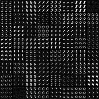
Figure 4 shows a qualitative comparison between MMVAE trained with the MoE objective in eq. 2 against the MVAE model of Wu and Goodman (2018). The MVAE was trained using the authors’ publicly available code, following their recommended training regime. We generate from the model $p_{{\Theta}}\left(\bm{z},\bm{x}_{1:M}\right)$ by taking $R=64$ samples from the prior $\bm{z}\sim p\left(\bm{z}\right)$, each of which is used to take $N=9$ samples from the likelihood of each modality $m$ as $x_{m}\,\hstretch{0.9}{\vstretch{0.9}{\sim}}\,p_{{\Theta}}\left(\bm{x}_{m}\mid\bm{z}\right)$. Note the quality of the MMVAE model, both at coherent joint generation (top row)—where corresponding samples for the same $\bm{z}$ match in their digits—and at coherent cross-generation (middle and bottom rows). To show that it is truly the MoE factorisation that impacts the learning—rather than our particular choice of model architecture or the IWAE objective—we explore performance on only adopting MoE, directly in the codebase of Wu and Goodman (2018), keeping all other aspects fixed, in Appendix E. Results indicate MVAE with the MoE posterior does appear to do better, especially at cross-modal generation, than the PoE.

Figure 5: Per-dimension latent traversals for a pair of datapoints indicating dimensions that affect only SVHN, only MNIST, and both MNIST & SVHN.

We subsequently analyse the structure of the latent space by traversing each dimension independently as shown in Figure 5. Here, for each modality $m$, we encode datapoint $\bm{x}_{m}$ through its respective encoder $q_{{\phi_{m}}}\left(\bm{z}\mid\bm{x}_{m}\right)$ to obtain the mean embedding $\mu_{m}$. Then, we perturb the embedding value along each dimension $\mu_{m}^{d}$ linearly in the range $(\mu_{m}^{d}-5\sigma_{0}^{d},\mu_{m}^{d}+5\sigma_{0}^{d})$, where $\sigma_{0}^{d}$ is the learnt standard deviation for dimension $d$ in the prior $p\left(\bm{z}\right)$. Note the extent to which particular dimensions affect only a single modality, whereas other dimensions affect both, indicating a degree of latent factorisation. Also shown is a plot of the per-dimension Kullback-Leibler divergence (KL) between each posterior and the prior, as well as the symmetric KL between the two posteriors, to indicate which dimensions encode information from which posterior, if any.

Quantitative Results:

To quantify the extent to which the latent spaces factorises from multi-modal observations, we employ a simple linear classifier on the latent representations as we have no a-priori reason to believe that the representations factorise in an axis-aligned manner. If a linear digit classifier can extract the digit information from the shared latent space, it strongly indicates the presence of a linear subspace that has factored as desired. We train digit classifiers for a) MMVAE, b) MVAE, with posterior either from single-modality inputs or multi-modality inputs, and c) single-VAE that takes input from one modality only, plotting results in Table 1. Comparing the results of the first column to the last in Table 1, we find MMVAE’s latent space provides significantly better accuracy over the single-VAE. For the MVAE, due to its PoE formulation, it appears that the MNIST modality dominates, obtaining high accuracy for MNIST digit classification (95.7%) but low for SVHN (9.10%). When given both inputs, accuracy for SVHN improves significantly while that for MNIST decreases slightly. Note that the accuracy for MVAE is higher when only the MNIST data is presented compared to when both modalities are available, indicating that the presence of the extra modality does not further inform the model on the classification of digits.

Table 1: Digit classification accuracy (%) of latent variables in different models.

	MMVAE	MVAE (single)	MVAE (both)	single-VAE
MNIST	$91.3$	$95.7$	$94.9$	$85.3$
SVHN	$68.0$	$9.1$	$90.1$	$20.7$

We also quantify the coherence of joint generations and cross-modal generations. To do so, we employ off-the-shelf digit classifiers of the original MNIST and SVHN datasets on the generation results, and compute a) for joint generation, how often the digits of generations in two modalities match, and b) for cross-modal generation, how often the digit generated in one modality matches its input from another modality. Results in Table 2 indicate that for joint generation, the classifiers predict the same digit class 42.1% of time, and for cross-generation, 86.4% (MNIST $\rightarrow$SVHN) and 69.1% (SVHN $\rightarrow$ MNIST). Computing these metrics for MVAE yields accuracy close to chance, suggesting that the coherence between modalities is not quite preserved when considering generation.

Table 2: Probability of digit matching (%) for joint and cross generation.

	Joint	Cross (M$\rightarrow$S)	Cross (S$\rightarrow$M)
MMVAE	$42.1$	$86.4$	$69.1$
MVAE	$12.7$	$9.5$	$9.3$

We finally compute the marginal likelihoods of the joint generative model $p_{{\Theta}}\left(\bm{x}_{1:M}\right)$, and each of the individual generative models $p_{{\theta_{m}}}\left(x_{m}\right)$ using both the joint variational posterior $q_{{\Phi}}\left(\bm{z}\mid\bm{x}_{1:M}\right)$ and the single variational posterior $q_{{\phi_{m}}}\left(\bm{z}\mid x_{m}\right)$ as shown in Table 3.

Table 3: Evaluating the different log likelihoods for different arrangements of MNIST and SVHN.

		$\log p(\bm{x}_{m},\bm{x}_{n})$	$\log p(\bm{x}_{m}\mid\bm{x}_{m},\bm{x}_{n})$	$\log p(\bm{x}_{m}\mid\bm{x}_{m})$	$\log p(\bm{x}_{m}\mid\bm{x}_{n})$
$m={}$MNIST, $n={}$SVHN	MMVAE	$6261.40$	$868.76$	$868.37$	$628.31$
	MVAE	$2961.80$	$-176.68$	$-107.46$	$-778.20$
$m={}$SVHN, $n={}$MNIST	MMVAE	$6261.40$	$3441.01$	$3441.01$	$2337.56$
	MVAE	$2961.80$	$3395.12$	$3536.86$	$-12747.50$

We observe that MMVAE model yields higher likelihoods, consistent with employing the IWAE estimator. Interestingly, we observe that $p(\bm{x}_{m}\mid\bm{x}_{m},\bm{x}_{n})\geq p(\bm{x}_{m}\mid\bm{x}_{m})$ for MMVAE, whereas for MVAE we consistently find $p(\bm{x}_{m}\mid\bm{x}_{m},\bm{x}_{n})<p(\bm{x}_{m}\mid\bm{x}_{m})$. This serves to highlights that the MMVAE model is able to effectively utilise information jointly across multiple modalities, which the MVAE model potentially suffers from overdominant encoders and an ill-suited sub-sampled training scheme to accommodate data always present across modalities at train time.

4.3 CUB Image-Captions

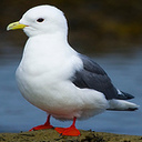	the bird has a white body, black wings, and webbed orange feet
	a blue bird with gray primaries and secondaries and white breast and throat

Figure 6: Example data

Dataset:

Encouraged by the results from our previous experiment, we consider a multi-modal experiment more in line with our original motivation. We employ the images and captions from Caltech-UCSD Birds (CUB) dataset (Wah et al., 2011), containing 11,788 photos of birds in natural scenes, each annotated with 10 fine-grained captions describing the bird’s appearance characteristics collected through Amazon Mechanical Turk (AMT). As shown in Figure 6, the images are quite detailed and descriptions fairly complex, involving the composition of various attributes. For the image data, rather than generating directly in image space, we instead generate in the feature space of a pre-trained ResNet-101 (He et al., 2016), in order to avoid issues with blurry generations for complex image data (Zhao et al., 2017). For generations and reconstructions, we simply perform a nearest-neighbour lookup in feature space using Euclidean distance on the generated or reconstructed feature. For the language data, we employ a CNN encoder and decoder following Kalchbrenner et al. (2014); Pham et al. (2016); Massiceti et al. (2018b), learning an embedding for words in the process. We use 128-dimensional latents with a Laplace likelihood on image features and a Categorical likelihood for captions.

Figure 7: Qualitative evaluation of the MMVAE model on the CUB data, showing reconstruction in the individual modalities (top rows), cross generation (middle and bottom rows on right), and joint generation (bottom row on left). More qualitative examples can be found in Appendix G.

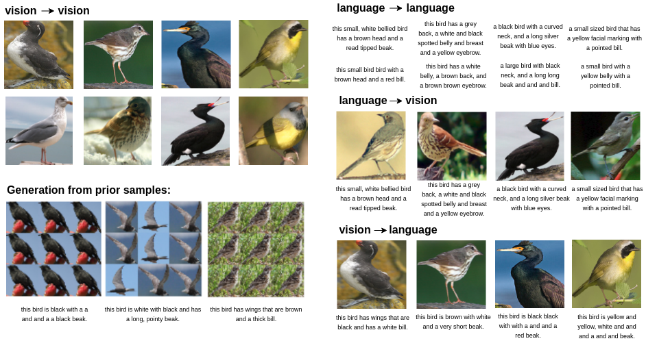
Qualitative Results:

Figure 7 shows qualitative results for the MMVAE model trained with the MoE objective in eq. 2 on the CUB data. We generate from the model as before, with $R=4$, and $N_{1}=9,N_{2}=1$. Interestingly, even for such a complicated dataset, we see joint generation align quite well with descriptions largely in line with the image for a range of different attributes, and cross generation where the descriptions again match the image quite well and vice versa. An interesting avenue to explore for future directions in this experiment would be the incorporation of more complex generative models for images potentially incorporating the use of GANs to improve the quality of generated output, and observing its effect on the joint modelling. We also generate results for MVAE on this dataset, where we observe that the image modality dominates and resulting in poor language reconstruction and cross-modal generation. See Appendix H for examples and further details.

Quantitative Results:

We evaluate the coherence of our generation by calculating the correlation between the jointly and cross-generated image-caption pair. We do so by employing Canonical Correlation Analysis (CCA) following the observation of its effectiveness as a baseline for language and vision tasks by Massiceti et al. (2018a). Here, given paired observations $\{x_{1}\in\mathbb{R}^{n_{1}},x_{2}\in\mathbb{R}^{n_{2}}\}$, CCA learns projections $W_{1}\in\mathbb{R}^{n_{1}\times k}$ and $W_{2}\in\mathbb{R}^{n_{2}\times k}$ that maximise the correlation between projected variables $W_{1}^{T}x_{1}$ and $W_{2}^{T}x_{2}$. With this formulation, the correlation between any new pair of observations $\{\tilde{x}_{1},\tilde{x}_{2}\}$ can be computed as the cosine distance between the mean-centered projected variables, i.e.

$$\text{corr}(\tilde{x}_{1},\tilde{x}_{2})=\frac{\phi(\tilde{x}_{1})^{T}\phi(\tilde{x}_{2})}{||\phi(\tilde{x}_{1})||_{2}||\phi(\tilde{x}_{2})||_{2}}$$ (3)

where $\phi(\tilde{x}_{n})=W_{n}^{T}\tilde{x}_{n}-\text{avg}(W_{n}^{T}x_{n})$.

We prepare the dataset for CCA by pre-processing both modalities using feature extractors. For images, similar to training, we use the off-the-shelf ResNet-101 to generate feature vector of dimension 2048-$d$; for captions, we fit a FastText model on all sentences in the training set, projecting each word onto a 300-$d$ vector (Bojanowski et al., 2017). The representation for each caption is then acquired by aggregating the embedding of all words in the sentence (here we simply take the average). To compute the correlation between the generated images and captions, we first compute the projection matrix $W$ for each modality using the training set of CUB Image-Captions, then perform CCA using eq. 3, on i) jointly generated image-sentence pairs, taking average over $1000$ examples, and ii) image-sentence or sentence-image pair of cross generation, taking an average over the entire test set. Results are as shown in Table 4.

Table 4: Correlation of Image (I)-Sentence (S) pair for joint and cross generation.

	Joint	Cross (I $\rightarrow$S)	Cross (S $\rightarrow$I)	Ground Truth
MMVAE	$0.263$	$0.104$	$0.135$	0.273
MVAE	$-0.095$	$0.011$	$-0.013$

Table 4 shows that the average correlation of joint generation of our model is $0.263$; This value is only slightly lower than the average correlation of the data itself ($0.273$ in Table 4), which demonstrates the high coherence between the jointly generated image-caption pairs. For cross-generation, the correlation between input images and generated captions is slightly lower than that of input caption and generated image, evaluated at $0.104$ and $0.135$ respectively.

In comparison, the MVAE model appears to provide (marginally) negative correlation for the jointly generated pairs and sentence $\rightarrow$ image cross generation pairs. Notably, the correlation for image $\rightarrow$ sentence generation is much higher than sentence $\rightarrow$ image ($0.011$ and -$0.013$ respectively). Observing the qualitative results for MVAE in Appendix H also shows that any outputs generated from images as input is more expressive than those from the language inputs. These findings indicate that the model places more weight on the image modality than language for the factorisation of joint posterior, once again indicating an overdominant encoder, providing empirical evidence for our analysis of the PoE’s potential bias towards stronger experts in § 3.

5 Conclusion

In this paper, we explore multi-modal generative models, characterising successful learning of such models as the fulfillment of four specific criteria: i) implicit latent decomposition into shared and private subspaces, ii) coherent simultaneous joint generation over all modalities, iii) coherent cross-generation between individual modalities, and iv) improved model learning for the individual modalities as a consequence of having observed data from different modalities. Satisfying these goals enables more useful and generalisable representations for downstream tasks such as classification, by capturing the abstract relationship between the modalities. To this end, we propose a variational mixture of experts (MoE)autoencoder framework that allows us to achieve these criteria, in contrast to prior work which primarily target just the cross-modal generation and improved model learning aspects. We compare and contrast our MMVAE model against the state-of-the-art product of experts (PoE)model of Wu and Goodman (2018) and demonstrate that we outperform it at satisfying these four criteria. We evaluate our model on two challenging datasets that capture both image $\leftrightarrow$ image and image $\leftrightarrow$ language transformations, showing appealing results across these tasks.

Acknowledgements

YS, NS, and PHST were supported by the ERC grant ERC-2012-AdG 321162-HELIOS, EPSRC grant Seebibyte EP/M013774/1 and EPSRC/MURI grant EP/N019474/1, with further support from the Royal Academy of Engineering and FiveAI. YS was additionally supported by Remarkdip through their PhD Scholarship Programme. BP is supported by the Alan Turing Institute under the EPSRC grant EP/N510129/1.

Appendix: Variational Mixture-of-Experts Autoencoders                      for Multi-Modal Deep Generative Models

Appendix A Tighter lower bound

With the MoE joint posterior, an alternative way of extending the $\mathcal{L}_{\lx@glossaries@gls@link{acronym}{IWAE}{\leavevmode\textsc{IWAE}}}$ in Equation 1 to $M$-modalities is by employing stratified sampling (Robert and Casella, 2013)—to take $K$ samples from the joint posterior, we first sample a modality $m$, then take $L=K/M$ samples from the corresponding marginal variational posterior $q_{{\phi_{m}}}\left(\bm{z}\mid\bm{x}_{m}\right)$, and repeat the process $M$ times. Formally,

$$\underline{\mathcal{L}}_{\lx@glossaries@gls@link{acronym}{IWAE}{\leavevmode\textsc{IWAE}}}^{\lx@glossaries@gls@link{acronym}{MoE}{\leavevmode\textsc{MoE}}}(\bm{x}_{1:M})=\operatorname{{}\mathbb{E}}_{\begin{subarray}{c}\bm{z}_{1}^{1:L}\,\hstretch{0.9}{\vstretch{0.9}{\sim}}\,q_{{\phi_{1}}}\left(\bm{z}\mid\bm{x}_{1}\right)\\[-1.50694pt] \vdots\\ \bm{z}_{M}^{1:L}\,\hstretch{0.9}{\vstretch{0.9}{\sim}}\,q_{{\phi_{M}}}\left(\bm{z}\mid\bm{x}_{M}\right)\end{subarray}}\left[\log\frac{1}{M}\sum_{m=1}^{M}\frac{1}{L}\sum_{l=1}^{L}\frac{p_{{\Theta}}\left(\bm{z}_{m}^{l},\bm{x}_{1:M}\right)}{q_{{\Phi}}\left(\bm{z}_{m}^{l}\mid\bm{x}_{1:M}\right)}\right].$$ (7)

Applying Jensen’s inequality, we see that Equation 7 is a tighter lower bound than Equation 2; that is, $\mathcal{L}_{\lx@glossaries@gls@link{acronym}{IWAE}{\leavevmode\textsc{IWAE}}}^{\lx@glossaries@gls@link{acronym}{MoE}{\leavevmode\textsc{MoE}}}(\bm{x}_{1:M})\leq\underline{\mathcal{L}}_{\lx@glossaries@gls@link{acronym}{IWAE}{\leavevmode\textsc{IWAE}}}^{\lx@glossaries@gls@link{acronym}{MoE}{\leavevmode\textsc{MoE}}}(\bm{x}_{1:M})\leq\log p_{{\Theta}}\left(\bm{x}_{1:M}\right)$; however, it can adversely affect the ability to perform cross-modal generation. To see this, consider the form of the gradient estimator of this objective with respect to the variational posterior parameters $\Phi$ (Burda et al., 2015; Cremer et al., 2017),

$$\nabla_{\Phi}\underline{\mathcal{L}}_{\lx@glossaries@gls@link{acronym}{IWAE}{\leavevmode\textsc{IWAE}}}^{\lx@glossaries@gls@link{acronym}{MoE}{\leavevmode\textsc{MoE}}}(\bm{x}_{1:M})=\operatorname{{}\mathbb{E}}_{\epsilon^{1:K}\,\hstretch{0.9}{\vstretch{0.9}{\sim}}\,p(\epsilon)}\left[\sum_{k}\bar{w}^{k}\nabla_{\Phi}\log w^{k}\right],$$ (8)

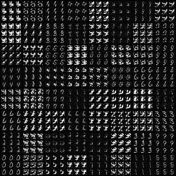
where $K=ML$, $\bm{z}^{k}=g(\epsilon^{k},\Phi)$ (reparameterised), $w^{k}=\frac{p_{{\Theta}}\left(\bm{z}^{k},\bm{x}_{1:M}\right)}{q_{{\Phi}}\left(\bm{z}^{k}\mid\bm{x}_{1:M}\right)}$, and $\bar{w}^{k}=\frac{w^{k}}{\sum_{j=1}^{K}w^{j}}$, indicating that the gradient weights samples by their relative importance $\bar{w}^{k}$. Two different samples $\bm{z}^{k_{1}}$, and $\bm{z}^{k_{2}}$ coming from different modalities (encoders) can have their gradients weighed differently from one another, leading to situations where the joint variational posterior collapses to one of the experts in the mixture. Figure 8 shows empirical evidence of this happening, comparing performance under Equations 7 and 2 for the same data.

Generations MNIST [1mm] $\rightarrow$$\ast$ SVHN [1mm] $\rightarrow$$\ast$	$\mathcal{L}_{\lx@glossaries@gls@link{acronym}{IWAE}{\leavevmode\textsc{IWAE}}}^{\lx@glossaries@gls@link{acronym}{MoE}{\leavevmode\textsc{MoE}}}(\bm{x}_{1:M})$	$\underline{\mathcal{L}}_{\lx@glossaries@gls@link{acronym}{IWAE}{\leavevmode\textsc{IWAE}}}^{\lx@glossaries@gls@link{acronym}{MoE}{\leavevmode\textsc{MoE}}}(\bm{x}_{1:M})$

Figure 8: Comparing performance for MNIST-SVHN between the $\mathcal{L}_{\lx@glossaries@gls@link{acronym}{IWAE}{\leavevmode\textsc{IWAE}}}^{\lx@glossaries@gls@link{acronym}{MoE}{\leavevmode\textsc{MoE}}}(\bm{x}_{1:M})$ and $\underline{\mathcal{L}}_{\lx@glossaries@gls@link{acronym}{IWAE}{\leavevmode\textsc{IWAE}}}^{\lx@glossaries@gls@link{acronym}{MoE}{\leavevmode\textsc{MoE}}}(\bm{x}_{1:M})$ objectives.

Compared to the original objective (LHS), the cross generation of $\widehat{\mathcal{L}}_{\lx@glossaries@gls@link{acronym}{IWAE}{\leavevmode\textsc{IWAE}}}^{\lx@glossaries@gls@link{acronym}{MoE}{\leavevmode\textsc{MoE}}}(\bm{x}_{1:M})$ struggles to match digits between the modalities, especially in the SVHN $\rightarrow$ MNIST case. Coherence for joint generation is also worse, with no recognisable matching-up of digits between the two modalities. Similar to Table 2, we evaluate the coherence of cross and joint generation by computing the accuracy of digit predictions between the two modalities in Table 5. Note the drop in performance for the $\underline{\mathcal{L}}_{\lx@glossaries@gls@link{acronym}{IWAE}{\leavevmode\textsc{IWAE}}}^{\lx@glossaries@gls@link{acronym}{MoE}{\leavevmode\textsc{MoE}}}(\bm{x}_{1:M})$ objective reflecting the qualitative results.

Objective	Joint	Cross (M $\rightarrow$S)	Cross (S $\rightarrow$M)
$\mathcal{L}_{\lx@glossaries@gls@link{acronym}{IWAE}{\leavevmode\textsc{IWAE}}}^{\lx@glossaries@gls@link{acronym}{MoE}{\leavevmode\textsc{MoE}}}(\bm{x}_{1:M})$	$42.1$	$86.4$	$69.1$
$\underline{\mathcal{L}}_{\lx@glossaries@gls@link{acronym}{IWAE}{\leavevmode\textsc{IWAE}}}^{\lx@glossaries@gls@link{acronym}{MoE}{\leavevmode\textsc{MoE}}}(\bm{x}_{1:M})$	$24.2$	$74.6$	$15.6$

Table 5: Probability of digit matching (%) for joint and cross generation.

Appendix B Multi-Modal Importance-Sampled ELBO

Consider the ELBO, with the basic MoE variational posterior,

$$\mathcal{L}_{\operatorname{\lx@glossaries@gls@link{acronym}{ELBO}{\leavevmode\textsc{ELBO}}}}(\bm{x}_{1:M}) =\frac{1}{M}\sum_{m=1}^{M}\operatorname{{}\mathbb{E}}_{z\sim q_{\phi_{m}}(\bm{z}\mid\bm{x}_{m})}\left[\log\frac{p_{\Theta}(\bm{z},\bm{x}_{1:M})}{q_{{\Phi}}\left(\bm{z}\mid\bm{x}_{1:M}\right)}\right].$$

The term corresponding to a particular modality $i$ is given as

$$\operatorname{{}\mathbb{E}}_{\bm{z}_{i}\sim q_{\phi_{i}}(\bm{z}\mid\bm{x}_{i})}\left[\log\frac{p_{{\Theta}}\left(\bm{z}_{i},\bm{x}_{1},\ldots,\bm{x}_{i},\ldots,\bm{x}_{M}\right)}{q_{{\Phi}}\left(\bm{z}_{i}\mid\bm{x}_{1:M}\right)}\right]$$

$$=\operatorname{{}\mathbb{E}}_{\bm{z}_{i}\sim q_{\phi_{i}}(\bm{z}\mid\bm{x}_{i})}\left[\log\frac{p_{{\Theta}}\left(\bm{z}_{i},\bm{x}_{i}\right)}{q_{{\Phi}}\left(\bm{z}_{i}\mid\bm{x}_{1:M}\right)}\right]+\sum_{\begin{subarray}{c}j=1\\ j\neq i\end{subarray}}^{M}\operatorname{{}\mathbb{E}}_{\bm{z}_{i}\sim q_{\phi_{i}}(\bm{z}\mid\bm{x}_{i})}\left[\log p_{\theta_{j}}(\bm{x}_{j}\mid\bm{z}_{i})\right]$$

$$=\operatorname{{}\mathbb{E}}_{\bm{z}_{i}\sim q_{\phi_{i}}(\bm{z}\mid\bm{x}_{i})}\left[\log\frac{p_{{\Theta}}\left(\bm{z}_{i},\bm{x}_{i}\right)}{q_{{\Phi}}\left(\bm{z}_{i}\mid\bm{x}_{1:M}\right)}\right]+\sum_{\begin{subarray}{c}j=1\\ j\neq i\end{subarray}}^{M}\underbrace{\operatorname{{}\mathbb{E}}_{\bm{z}_{j}\sim\bar{q}_{\phi_{j}}(\bm{z}\mid\bm{x}_{j})}\left[\frac{q_{\phi_{i}}(\bm{z}_{j}\mid\bm{x}_{i})}{\bar{q}_{\phi_{j}}(\bm{z}_{j}\mid\bm{x}_{j})}\log p_{\theta_{j}}(\bm{x}_{j}\mid\bm{z}_{j})\right]}_{A_{j}}$$

where $\bar{q}$ does not propagate gradients (effectively issuing a stop_gradient), since all the likelihoods in the second term only have gradients with respect to $\phi_{i},\theta_{j},j\neq i$ . Each term $A_{j}$ can be seen as an importance-sampled estimate of $\displaystyle\operatorname{{}\mathbb{E}}_{\bm{z}_{i}\sim q_{\phi_{i}}(\bm{z}|\bm{x}_{i})}\left[\log p_{{\theta_{j}}}\left(\bm{x}_{j}\mid\bm{z}_{i}\right)\right]$ using that modality $j$’s own encoding distribution $q_{{\phi_{j}}}\left(\bm{z}_{j}\mid\bm{x}_{j}\right)$. This has two major benefits:

1. it allows the total objective to be computed with just a single pass over each encoder and decoder to make computation linear in $M$. To see this is true, note that one can effectively precompute the likelihoods of modality $j$ using samples from its own encoder, and simply weigh them by the appropriate ratio of variational posteriors where necessary.

2. estimating the likelihood of modality $j$ using samples from modality $i$, where $i\neq j$, is a difficult ask—since observation $\bm{x}_{i}$ only carries partial information applicable for the reconstruction of $\bm{x}_{j}$. This multi-modal importance sampling sidesteps the issue by using samples from same modality $j$, with appropriate weighting. We would expect this to generally thus produce a lower-variance estimator, as it avoids potentially evaluating $\log p_{\theta_{j}}(\bm{x}_{j}\mid\bm{z}_{i})$ for values $\bm{z}_{i}$ which yield very low likelihoods on $\bm{x}_{j}$. Moreover, since the denominators of the importance ratios cannot propagate gradients, the only way to improve the estimate is by maximising the density of samples from modality $j$ in the variational posterior for $i$ as $q_{{\phi_{i}}}\left(\bm{z}_{j}\mid\bm{x}_{i}\right)$, bringing the different components closer to each other.

Appendix C The DReG Estimator

The standard gradient estimator of IWAE can have undesirably high variance (Roeder et al., 2017; Rainforth et al., 2018). To see this, we can expand Equation 8 as:

$$\nabla_{\Phi}\operatorname{{}\mathbb{E}}_{z^{1:K}}\left[\log\left(\frac{1}{K}\sum_{k=1}^{K}w^{k}\right)\right]=\operatorname{{}\mathbb{E}}_{\epsilon^{1:K}}\left[\sum_{k=1}^{K}\frac{w^{k}}{\sum_{j=1}^{K}w^{j}}\left(-\frac{\partial}{\partial\Phi}\log q_{{\Phi}}\left(\bm{z}^{k}\mid\bm{x}\right)+\frac{\partial\log w^{k}}{\partial\bm{z}^{k}}\frac{d\bm{z}^{k}}{d\Phi}\right)\right]$$ (25)

Roeder et al. (2017) find that when $K>1$, the first term within paranthesis in Equation 25 need not be zero even when the approximate posterior matches true posterior everywhere, which can contribute to significant variance in the gradient estimator. To alleviate this, Tucker et al. (2019) re-apply the reparametrisation trick on it, yielding a doubly reparametrised gradient estimator (DReG):

$$\nabla_{\Phi}E_{z^{1:K}}\left[\log\left(\frac{1}{K}\sum_{k=1}^{K}w^{k}\right)\right]=E_{\epsilon^{1:K}}\left[\sum_{k=1}^{K}\left(\frac{w^{k}}{\sum_{j=1}^{K}w^{j}}\right)^{2}\frac{\partial\log w^{k}}{\partial\bm{z}^{k}}\frac{d\bm{z}^{k})}{d\Phi}\right]$$ (26)

We implement the estimator specified in Equation 26 when performing gradient updates for any experiment involving the IWAE objective.

Appendix D Higher entropy of IWAE variational posteriors

To see why the variational posteriors estimated by IWAE tend to have higher entropy than those by ELBO, it is beneficial to consider the objectives from a different perspective.

First, let’s take a look at ELBO: maximising the standard ELBO indirectly minimises the KL between the variational and true posteriors, since

$$\log p_{{\Theta}}\left(\bm{x}_{1:M}\right)=\mathcal{L}_{\operatorname{\lx@glossaries@gls@link{acronym}{ELBO}{\leavevmode\textsc{ELBO}}}}(\bm{x}_{1:M})+\operatorname{\scalebox{0.95}{\text{KL}}}\left(q_{{\Phi}}\left(\bm{z}\mid\bm{x}_{1:M}\right)\,\|\;p_{{\Theta}}\left(\bm{z}\mid\bm{x}_{1:M}\right)\right).$$

Maximising the IWAE objective however, indirectly minimises the KL between implicit posteriors (Le et al., 2018) as

$$\log p_{{\Theta}}\left(\bm{x}_{1:M}\right)=\mathcal{L}_{\lx@glossaries@gls@link{acronym}{IWAE}{\leavevmode\textsc{IWAE}}}(\bm{x}_{1:M})+\operatorname{\scalebox{0.95}{\text{KL}}}\left(q_{{\Phi^{IS}}}\left(\bm{z}\mid\bm{x}_{1:M}\right)\,\|\;p_{{\Theta^{IS}}}\left(\bm{z}\mid\bm{x}_{1:M}\right)\right),$$

where

$$p_{{\Theta^{IS}}}\left(\bm{z}\mid\bm{x}_{1:M}\right) =\frac{1}{K}\sum_{k}\frac{q_{{\Phi^{IS}}}\left(\bm{z}\mid\bm{x}_{1:M}\right)}{q_{{\Phi}}\left(\bm{z}^{k}\mid\bm{x}_{1:M}\right)}p_{{\Theta}}\left(\bm{z}^{k}\mid\bm{x}_{1:M}\right),$$

$$q_{{\Phi^{IS}}}\left(\bm{z}\mid\bm{x}_{1:M}\right) =\frac{1}{K}\prod_{k}q_{{\Phi}}\left(\bm{z}^{k}\mid\bm{x}_{1:M}\right),$$

leading to higher-entropy estimates of the variational posterior.

This suits the learning of multi-modal data as each modality’s posterior attempts to explain more than just its own modality.

Appendix E Qualitative results of MVAE implementation with MoE posterior

Generations MNIST [1mm] $\rightarrow$$\ast$ SVHN [1mm] $\rightarrow$$\ast$

MVAE (original, PoE) MVAE (MoE)

Figure 9: A comparison of PoE vs. MoE in the MVAE codebae.

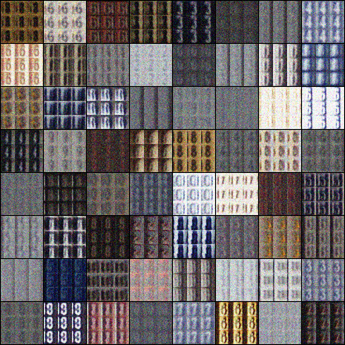
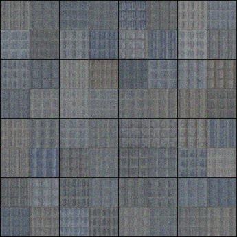
Here we show a qualitative evaluation in the MVAE codebase, minimally altered to use a MoE joint approximate posterior, with the results of the original PoE-MVAE model as a comparison. We can see that MoE is able to generate recognisable MNIST digits from SVHN inputs (bottom row, column 3), while the original model fails completely at cross-modal generation. Although, do note that neither model performs well at coherence joint generation (top row).

Appendix F Encoder and decoder architectures

Encoder	Decoder
Input $\in\mathbb{R}^{1x28x28}$	Input $\in\mathbb{R}^{L}$
FC. 400 ReLU	FC. 400 ReLU
FC. $L$, FC. $L$	FC. 1 x 28 x 28 Sigmoid

(a) MNIST dataset.

Encoder	Decoder
Input $\in\mathbb{R}^{2048}$	Input $\in\mathbb{R}^{L}$
FC. 1024 ELU	FC. 256 ELU
FC. 512 ELU	FC. 512 ELU
FC. 256 ELU	FC. 1024 ELU
FC. $L$, FC. $L$	FC. 2048

(c) CUB image dataset.

Encoder
Input $\in\mathbb{R}^{1590}$
Word Emb. 256
4x4 conv. 32 stride 2 pad 1 & BatchNorm2d & ReLU
4x4 conv. 64 stride 2 pad 1 & BatchNorm2d & ReLU
4x4 conv. 128 stride 2 pad 1 & BatchNorm2d & ReLU
1x4 conv. 256 stride 1x2 pad 0x1 & BatchNorm2d & ReLU
1x4 conv. 512 stride 1x2 pad 0x1 & BatchNorm2d & ReLU
4x4 conv. L stride 1 pad 0, 4x4 conv. L stride 1 pad 0
Decoder
Input $\in\mathbb{R}^{L}$
4x4 upconv. 512 stride 1 pad 0 & ReLU
1x4 upconv. 256 stride 1x2 pad 0x1 & BatchNorm2d & ReLU
1x4 upconv. 128 stride 1x2 pad 0x1 & BatchNorm2d & ReLU
4x4 upconv. 64 stride 2 pad 1 & BatchNorm2d & ReLU
4x4 upconv. 32 stride 2 pad 1 & BatchNorm2d & ReLU
4x4 upconv. 1 stride 2 pad 1 & ReLU
Word Emb.T 1590

(d) CUB-Language dataset.

Table 6: Encoder and decoder architectures.

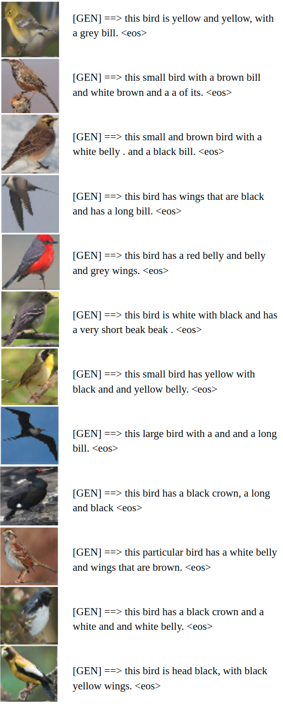
Appendix G Qualitative results of MMVAE on CUB

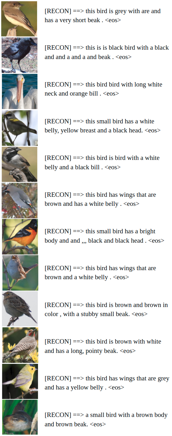
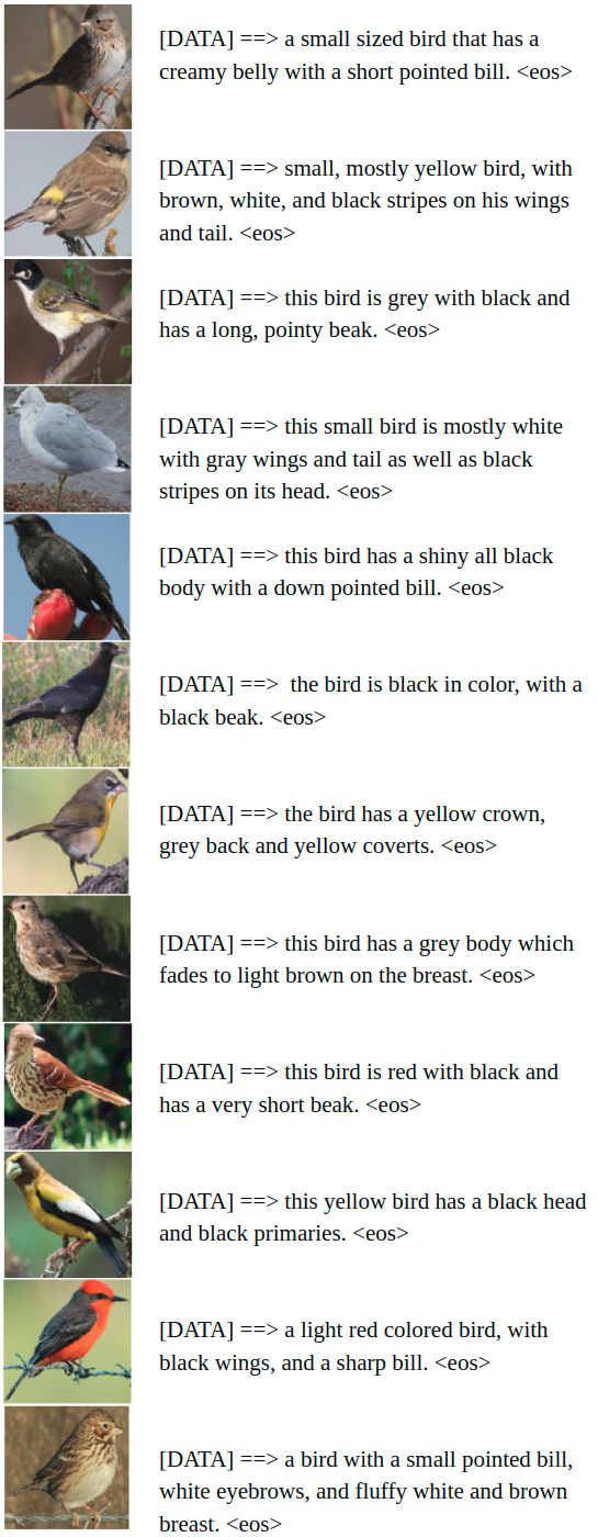
In this section, we show some more qualitative results of our MMVAE model on CUB Image-Caption dataset.

Figure 10: Image reconstruction of MMVAE on CUB Image-Caption dataset. Top row: ground truth, bottom row: reconstruction.

Figure 11: Caption reconstruction of MMVAE on CUB Image-Caption dataset.

(a) Image $\rightarrow$ Caption

(b) Caption $\rightarrow$ Image

(c) Joint Generation

Figure 12: Cross generation (a, b) and joint generation from prior samples (c) of MMVAE on CUB Image-Caption dataset.

Appendix H Qualitative results of Wu and Goodman (2018)’s MVAE on CUB

The qualitative results of MVAE on CUB Image-Caption dataset are as shown in Figure 13 and Figure 14. Note that similar to the MMVAE experiments, for the generation in the vision modality, we reconstruct the image features extracted from ResNet101 and perform nearest neighbour search to find the corresponding images.

Figure 13: Qualitative results of MVAE on CUB Image-Caption dataset, including reconstruction (vision $\rightarrow$ vision, language $\rightarrow$ language), cross generation (vision $\rightarrow$ language, language $\rightarrow$ vision) and joint generation from prior samples.

Figure 14: Qualitative results of MVAE on CUB Image-Caption dataset. Here both modalities are given to reconstruct the inputs.

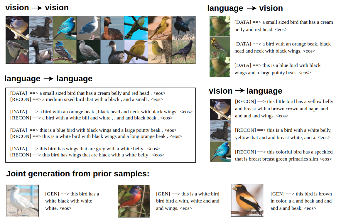
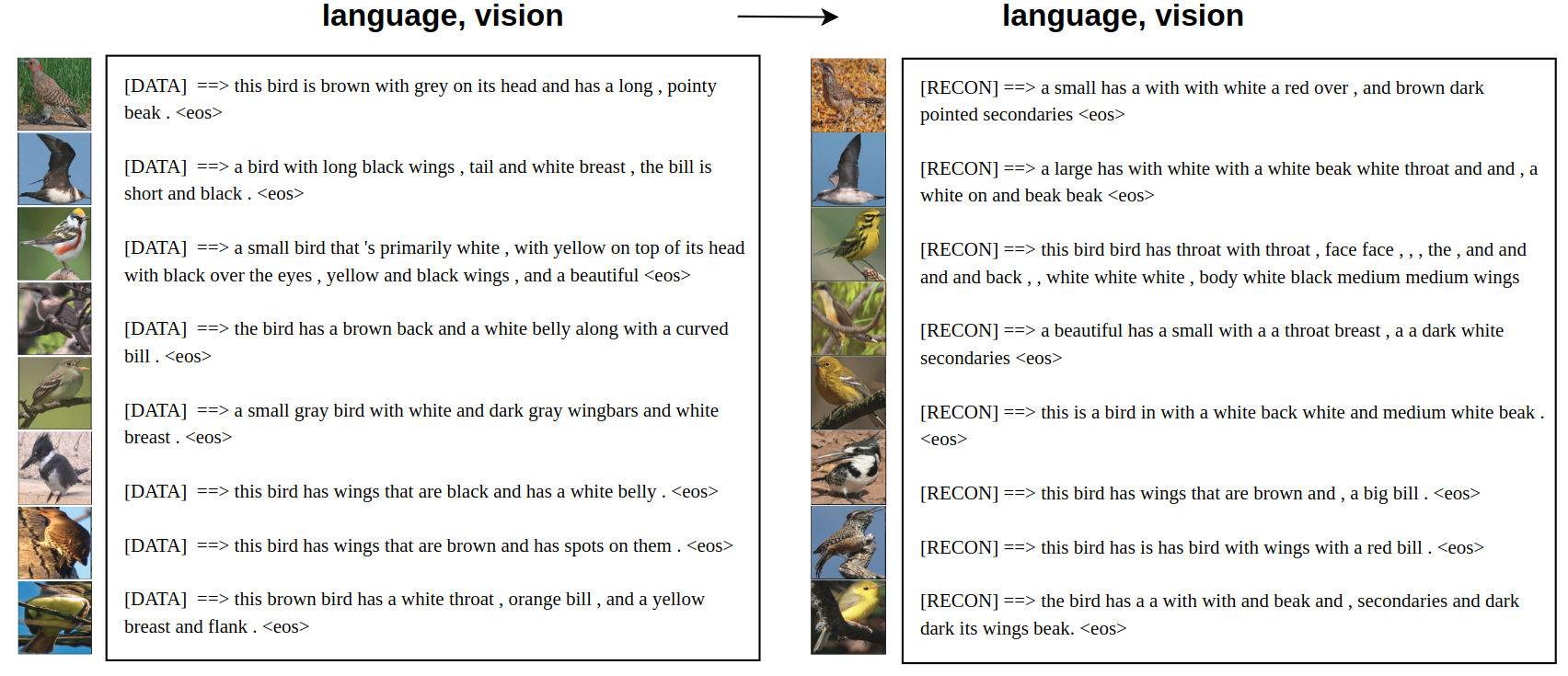
We can see from the results in Figure 13 that the vision modality dominates, with almost perfect image feature reconstruction; however, the performance in all other tasks are quite poor, especially when language is given as input: the language reconstruction fails to recover some of the key characteristics of the original description, replacing “small sized” with “medium sized”, “blue bird” with “white bird” etc.; the language-vision cross generation suffers from mode collapse, generating exclusively the 2 images under the language $\rightarrow$ vision column in Figure 13 for any given caption.

The language generation both in reconstruction (language $\rightarrow$ language) and cross-modal generation (vision $\rightarrow$ language) fails to capture the key characteristics the original caption; neither are joint generation of image-caption pairs coherent,. No significant improvement in reconstruction quality can be observed when both modalities are given as input, as seen in Figure 14, with the language generation omitting/“making up” important characteristics of the bird images. Performing CCA analysis on these image-caption pairs gives a negative correlation of -$0.00523$ (averaged over the test set), suggesting low coherence of the generated multi-modal data.

References

- Barnard et al. (2003) K. Barnard, P. Duygulu, D. Forsyth, N. d. Freitas, D. M. Blei, and M. I. Jordan. Matching words and pictures. Journal of machine learning research, 3(Feb):1107–1135, 2003.
- Barsalou (2008) L. W. Barsalou. Grounded cognition. Annual Review of Psychology, 59:617–645, 2008.
- Bauer and Johnson-Laird (1993) M. I. Bauer and P. N. Johnson-Laird. How diagrams can improve reasoning. Psychological science, 4(6):372–378, 1993.
- Blei and Jordan (2003) D. M. Blei and M. I. Jordan. Modeling annotated data. In Proceedings of the 26th annual international ACM SIGIR conference on Research and development in informaion retrieval, pages 127–134. ACM, 2003.
- Bojanowski et al. (2017) P. Bojanowski, E. Grave, A. Joulin, and T. Mikolov. Enriching word vectors with subword information. Transactions of the Association for Computational Linguistics, 5:135–146, 2017.
- Bousmalis et al. (2016) K. Bousmalis, G. Trigeorgis, N. Silberman, D. Krishnan, and D. Erhan. Domain separation networks. In Advances in Neural Information Processing Systems, pages 343–351, 2016.
- Burda et al. (2015) Y. Burda, R. Grosse, and R. Salakhutdinov. Importance weighted autoencoders. In International Conference on Learning Representations, 2015.
- Chu et al. (2017) C. Chu, A. Zhmoginov, and M. Sandler. Cyclegan, a master of steganography. arXiv preprint arXiv:1712.02950, 2017.
- Cremer et al. (2017) C. Cremer, Q. Morris, and D. Duvenaud. Reinterpreting importance-weighted autoencoders. In International Conference on Learning Representations (Workshop), 2017.
- Fan et al. (2018) J. E. Fan, D. Yamins, and N. B. Turk-Browne. Common object representations for visual recognition and production. Cognitive Science, 42:2670–2698, 2018.
- Ganin and Lempitsky (2015) Y. Ganin and V. Lempitsky. Unsupervised domain adaptation by backpropagation. In Proceedings of The 32nd International Conference on Machine Learning, pages 1180–1189, 2015.
- He et al. (2016) K. He, X. Zhang, S. Ren, and J. Sun. Deep residual learning for image recognition. In Proceedings of the IEEE conference on computer vision and pattern recognition, pages 770–778, 2016.
- Hinton (2002) G. E. Hinton. Training products of experts by minimizing contrastive divergence. Neural computation, 14(8):1771–1800, 2002.
- Kalchbrenner et al. (2014) N. Kalchbrenner, E. Grefenstette, and P. Blunsom. A convolutional neural network for modelling sentences. In Proceedings of the 52nd Annual Meeting of the Association for Computational Linguistics, pages 212–217. Association for Computational Linguistics, 2014.
- Kingma and Ba (2014) D. P. Kingma and J. Ba. Adam: a method for stochastic optimization. In International Conference on Learning Representations, 2014.
- Kingma and Welling (2014) D. P. Kingma and M. Welling. Auto-encoding variational bayes. In International Conference on Learning Representations, 2014.
- Le et al. (2018) T. A. Le, M. Igl, T. Rainforth, T. Jin, and F. Wood. Auto-encoding sequential monte carlo. In International Conference on Learning Representations, 2018.
- Ledig et al. (2017) C. Ledig, L. Theis, F. Huszár, J. Caballero, A. Cunningham, A. Acosta, A. Aitken, A. Tejani, J. Totz, Z. Wang, and W. Shi. Photo-realistic single image super-resolution using a generative adversarial network. In Proceedings of the IEEE Conference on Computer Vision and Pattern Recognition, pages 4681–4690, 2017.
- Li and Wand (2016) C. Li and M. Wand. Precomputed real-time texture synthesis with markovian generative adversarial networks. In European Conference on Computer Vision, pages 702–716. Springer, 2016.
- Lipton (2018) Z. C. Lipton. The mythos of model interpretability. ACM Queue, 61(10):36–43, 2018.
- Liu et al. (2017) M.-Y. Liu, T. Breuel, and J. Kautz. Unsupervised image-to-image translation networks. In Advances in neural information processing systems, pages 700–708, 2017.
- Liu et al. (2019) M.-Y. Liu, X. Huang, A. Mallya, T. Karras, T. Aila, J. Lehtinen, and J. Kautz. Few-shot unsupervised image-to-image translation, 2019.
- Long et al. (2015) M. Long, Y. Cao, J. Wang, and M. I. Jordan. Learning transferable features with deep adaptation networks. In Proceedings of the 32nd International Conference on Machine Learning, pages 97–105, 2015.
- Long et al. (2016) M. Long, H. Zhu, J. Wang, and M. I. Jordan. Unsupervised domain adaptation with residual transfer networks. In Advances in Neural Information Processing Systems, pages 136–144, 2016.
- Massiceti et al. (2018a) D. Massiceti, P. K. Dokania, N. Siddharth, and P. H. Torr. Visual dialogue without vision or dialogue. In NeurIPS Workshop on Critiquing and Correcting Trends in Machine Learning, 2018a.
- Massiceti et al. (2018b) D. Massiceti, N. Siddharth, P. K. Dokania, and P. H. Torr. FlipDial: a generative model for two-way visual dialogue. In IEEE Conference on Computer Vision and Pattern Recognition, 2018b.
- Mathieu et al. (2019) E. Mathieu, T. Rainforth, N. Siddharth, and Y. W. Teh. Disentangling disentanglement in variational autoencoders. In K. Chaudhuri and R. Salakhutdinov, editors, International Conference on Machine Learning (ICML), volume 97 of Proceedings of Machine Learning Research, pages 4402–4412, Long Beach, California, USA, June 2019. PMLR.
- Mukherjee et al. (2017) T. Mukherjee, M. Yamada, and T. M. Hospedales. Deep matching autoencoders. CoRR, abs/1711.06047, 2017.
- Ngiam et al. (2011) J. Ngiam, A. Khosla, M. Kim, J. Nam, H. Lee, and A. Y. Ng. Multimodal deep learning. In Proceedings of the 28th International Conference on Machine Learning, pages 689–696, 2011.
- Pandey and Dukkipati (2017) G. Pandey and A. Dukkipati. Variational methods for conditional multimodal deep learning. In International Joint Conference on Neural Networks, pages 308–315. IEEE, 2017.
- Pham et al. (2016) N.-Q. Pham, G. Kruszewski, and G. Boleda. Convolutional neural network language models. In Proceedings of the Conference on Empirical Methods in Natural Language Processing, pages 1153–1162, 2016.
- Pu et al. (2016) Y. Pu, Z. Gan, R. Henao, X. Yuan, C. Li, A. Stevens, and L. Carin. Variational autoencoder for deep learning of images, labels and captions. In D. D. Lee, M. Sugiyama, U. V. Luxburg, I. Guyon, and R. Garnett, editors, Advances in Neural Information Processing Systems, pages 2352–2360. Curran Associates, Inc., 2016.
- Quiroga et al. (2009) R. Q. Quiroga, A. Kraskov, C. Koch, and I. Fried. Explicit encoding of multimodal percepts by single neurons in the human brain. Current Biology, 19(15):1308–1313, 2009.
- Rainforth et al. (2018) T. Rainforth, A. R. Kosiorek, T. A. Le, C. J. Maddison, M. Igl, F. Wood, and Y. W. Teh. Tighter variational bounds are not necessarily better. International Conference on Machine Learning (ICML), 2018.
- Reddi et al. (2018) S. J. Reddi, S. Kale, and S. Kumar. On the convergence of adam and beyond. In International Conference on Learning Representations, 2018.
- Robert and Casella (2013) C. Robert and G. Casella. Monte Carlo statistical methods. Springer Science & Business Media, 2013.
- Roeder et al. (2017) G. Roeder, Y. Wu, and D. K. Duvenaud. Sticking the landing: Simple, lower-variance gradient estimators for variational inference. In I. Guyon, U. V. Luxburg, S. Bengio, H. Wallach, R. Fergus, S. Vishwanathan, and R. Garnett, editors, Advances in Neural Information Processing Systems 30, pages 6925–6934. Curran Associates, Inc., 2017.
- Silberer and Lapata (2014) C. Silberer and M. Lapata. Learning grounded meaning representations with autoencoders. In Proceedings of the 52nd Annual Meeting of the Association for Computational Linguistics, volume 1, pages 721–732, 2014.
- Siskind (1994) J. M. Siskind. Grounding language in perception. Artificial Intelligence Review, 8(5):371–391, Sep 1994.
- Sohn et al. (2015) K. Sohn, H. Lee, and X. Yan. Learning structured output representation using deep conditional generative models. In Advances in Neural Information Processing Systems, pages 3483–3491, 2015.
- Stein et al. (2009) B. E. Stein, T. R. Stanford, and B. A. Rowland. The neural basis of multisensory integration in the midbrain: its organization and maturation. Hearing research, 258(1-2):4–15, 2009.
- Suzuki et al. (2017) M. Suzuki, K. Nakayama, and Y. Matsuo. Joint multimodal learning with deep generative models. In International Conference on Learning Representations Workshop, 2017.
- Taigman et al. (2017) Y. Taigman, A. Polyak, and L. Wolf. Unsupervised cross-domain image generation. In International Conference on Learning Representations, 2017.
- Tian and Engel (2019) Y. Tian and J. Engel. Latent translation: Crossing modalities by bridging generative models. arXiv preprint arXiv:1902.08261, 2019.
- Tsai et al. (2019) Y. H. Tsai, P. P. Liang, A. A. Bagherzade, L.-P. Morency, and R. Salakhutdinov. Learning factorized multimodal representations. In International Conference on Learning Representations, 2019.
- Tucker et al. (2019) G. Tucker, D. Lawson, S. Gu, and C. J. Maddison. Doubly reparameterized gradient estimators for monte carlo objectives. In International Conference on Learning Representations, 2019.
- Tzeng et al. (2014) E. Tzeng, J. Hoffman, N. Zhang, K. Saenko, and T. Darrell. Deep domain confusion: Maximizing for domain invariance. arXiv preprint arXiv:1412.3474, 2014.
- Vedantam et al. (2018) R. Vedantam, I. Fischer, J. Huang, and K. Murphy. Generative models of visually grounded imagination. In International Conference on Learning Representations, 2018.
- Wah et al. (2011) C. Wah, S. Branson, P. Welinder, P. Perona, and S. Belongie. The Caltech-UCSD Birds-200-2011 Dataset. Technical Report CNS-TR-2011-001, California Institute of Technology, 2011.
- Wang et al. (2016) W. Wang, X. Yan, H. Lee, and K. Livescu. Deep variational canonical correlation analysis. arXiv preprint arXiv:1610.03454, 2016.
- Wang and Gupta (2016) X. Wang and A. Gupta. Generative image modeling using style and structure adversarial networks. In European Conference on Computer Vision, pages 318–335. Springer, 2016.
- Wu and Goodman (2018) M. Wu and N. Goodman. Multimodal generative models for scalable weakly-supervised learning. In Advances in Neural Information Processing Systems, pages 5580–5590, 2018.
- Yan et al. (2016) X. Yan, J. Yang, K. Sohn, and H. Lee. Attribute2image: Conditional image generation from visual attributes. In European Conference on Computer Vision, pages 776–791. Springer, 2016.
- Yildirim (2014) I. Yildirim. From perception to conception: learning multisensory representations. 2014.
- Zhao et al. (2017) S. Zhao, J. Song, and S. Ermon. Towards deeper understanding of variational autoencoding models. arXiv preprint arXiv:1702.08658, 2017.
- Zhu et al. (2017a) J.-Y. Zhu, T. Park, P. Isola, and A. A. Efros. Unpaired image-to-image translation using cycle-consistent adversarial networks. In Proceedings of the IEEE International Conference on Computer Vision, pages 2223–2232, 2017a.
- Zhu et al. (2017b) J.-Y. Zhu, R. Zhang, D. Pathak, T. Darrell, A. A. Efros, O. Wang, and E. Shechtman. Toward multimodal image-to-image translation. In Advances in Neural Information Processing Systems, pages 465–476, 2017b.