Large-$N$ expansion and $\theta$-dependence of $2d$ $CP^{N-1}$ models beyond the leading order

Abstract

We investigate the $\theta$-dependence of 2-dimensional $CP^{N-1}$ models in the large-$N$ limit by lattice simulations. Thanks to a recent algorithm proposed by M. Hasenbusch to improve the critical slowing down of topological modes, combined with simulations at imaginary values of $\theta$, we manage to determine the vacuum energy density up the sixth order in $\theta$ and up to $N=51$. Our results support analytic predictions, which are known up to the next-to-leading term in $1/N$ for the quadratic term in $\theta$ (topological susceptibility), and up to the leading term for the quartic coefficient $b_{2}$. Moreover, we give a numerical estimate of further terms in the $1/N$ expansion for both quantities, pointing out that the $1/N$ convergence for the $\theta$-dependence of this class of models is particularly slow.

1 Introduction

The existence of field configurations with non-trivial topology characterize the non-perturbative properties of QCD and QCD-like models, leading in particular to a non-trivial dependence on a possible coupling to the topological charge operator $q(x)$, the so-called $\theta$ parameter. A non-zero $\theta$ implies an additional factor $\exp(i\theta Q)$ in the path-integral of the theory, where $Q=\int d^{4}x\,q(x)$ is the global topological charge (winding number); since $Q$ is integer-valued for field configurations decaying fast enough at infinity, the theory is invariant under $\theta\to\theta+2\pi$, so that $\theta$ behaves as an angular variable. For small values of $\theta$, the free energy (vacuum energy) density $f(\theta)$ can be Taylor expanded around $\theta=0$, a common parameterization being Vicari and Panagopoulos (2009)

$$f(\theta)-f(0)=\frac{1}{2}\chi\theta^{2}\left(1+\sum_{n=0}^{\infty}b_{2n}\theta^{2n}\right)\,.$$ (1)

The expansion contains only even terms because $\theta$ breaks CP-symmetry explicitly and the theory is CP-invariant at $\theta=0$. The quadratic coefficient $\chi$ is the topological susceptibility and is related to the second cumulant of the topological charge distribution at $\theta=0$, while the coefficients $b_{2n}$ are related to higher-order cumulants of this distribution.

Since $\theta$-dependence is connected to intrinsically non-perturbative properties of Quantum Field Theories, a numerical approach based on lattice Monte Carlo simulations is the natural first-principle approach to its investigation. However, various analytical strategies permit to obtain useful information, at least in certain limits.

Semiclassical approaches to $\theta$-dependence consider classical configurations with non-trivial topology, like instantons and anti-instantons, and compute the path-integral by integrating fluctuations around such class of configurations. One usually considers configurations with just one instanton or anti-instanton, so that the whole information is contained in the single-instanton effective action. In this way, one obtains results valid for an ensemble of independent (non-interacting) instantons and anti-instantons (dilute instanton gas approximation or DIGA), leading to a universal dependence of the free energy $\theta$:

$$f(\theta)-f(0)=\chi(1-\cos\theta)\,.$$ (2)

This approximation is expected to work well at least in some regimes, like for $SU(N)$ Yang-Mills theories in the deconfined, high-temperature phase, where the typical instanton effective action gets large (because of asymptotic freedom) and topological charge fluctuations become rare and dilute.

On the other hand, DIGA is known to break down when instanton interactions cannot be neglected, like in the confined phase of QCD and similar models. In this regime, an alternative approach is represented by an expansion in the inverse of the number of field components, i.e. in $1/N$ for $SU(N)$ Yang-Mills theories or for $CP^{N-1}$ models. Under very general assumptions, like requiring the existence of a non-trivial dependence on $\theta$, large-$N$ expansion leads at least to semi-quantitative insights, like the prediction that the coefficients $b_{2n}$ in Eq. (1) be suppressed as $1/N^{2n}$ Witten (1980, 1998), which for $SU(N)$ Yang-Mills theories has been checked by lattice simulations during the last few years Del Debbio et al. (2002); D’Elia (2003); Giusti et al. (2007); Panagopoulos and Vicari (2011); Cè et al. (2015); Bonati et al. (2016a, 2013, b, 2018a).

The case of $CP^{N-1}$ models in two dimensions, which is the subject of the present investigation, is special, because the large-$N$ expansion permits to obtain for them, as for other vector-like models, also quantitative predictions. Leading order computations are available for $\chi$ D’Adda et al. (1978) and for all $b_{2n}$ coefficients Bonati et al. (2016b); Del Debbio et al. (2006a), and even next-to-leading corrections are known for the topological susceptibility Campostrini and Rossi (1991). Despite the fact that numerical simulations for these models are less demanding than those for $SU(N)$ Yang-Mills theories, lattice results have failed up to now to provide a clear confirmation of these quantitative analytical predictions, apart from the case of the leading $1/N$ term for $\chi$ Campostrini et al. (1992a); Vicari (1993); Del Debbio et al. (2004); Hasenbusch (2017). Numerical results appeared in some cases to be even inconsistent with next-to-leading predictions for $\chi$ Del Debbio et al. (2004); Hasenbusch (2017). A recent investigation Bonanno et al. (2019) pointed out that at least the consistency can be recovered once one takes into account further terms in the $1/N$ expansion. The purpose of the present investigation is to go beyond the simple consistency, trying to achieve a quantitative agreement between lattice computations and analytical predictions, at least for the next-to-leading correction to $\chi$ and for the leading term in the $b_{2}$ coefficient: in Ref. Bonanno et al. (2019) it was suggested that, in order to do so, one should explore $N=50$ or larger. At the same time, we would like to achieve a numerical estimate of the further terms in the $1/N$ expansion for both quantities.

In order to achieve our goal, we have pushed our investigation up to $N=51$, where however standard algorithms face severe critical slowing down problems in the decorrelation of the topological charge Del Debbio et al. (2004), which can only partially be ameliorated by numerical strategies like simulated (or parallel) tempering in the coupling of the theory Vicari (1993); Bonanno et al. (2019). For this reason, we have decided to adopt an algorithm recently introduced by M. Hasenbusch in Ref. Hasenbusch (2017), in which simulations with open and periodic boundary conditions are smartly combined in a parallel tempering framework. In addition to that, following the same strategy adopted in Ref. Bonanno et al. (2019), we will assume analyticity around $\theta=0$ and exploit simulations performed at imaginary values of $\theta$ in order to improve the signal-to-noise ratio, something which turns out to be essential in order to achieve a precise determination of the higher-order cumulants of $Q$.

The paper is organized as follows. In Section 2 we provide a concise review of $CP^{N-1}$ models and of large-$N$ predictions for their $\theta$-dependence. In Section 3 we give details about the lattice discretization and the numerical algorithm employed in our study. Numerical results and their analysis within the framework of the $1/N$ expansion are presented in Section 4. Finally, in Section 5, we give our conclusions.

2 $CP^{N-1}$ models and their $\theta$-dependence in the large-$N$ limit

$CP^{N-1}$ models in two space-time dimensions share many properties with Yang-Mills theories: apart from $\theta$-dependence, they are also characterized by confinement of fundamental matter fields; for this reason they have represented a theoretical test-bed for the study of non-perturbative physics in gauge theories since long Witten (1979); D’Adda et al. (1978); David (1984); Shifman (2012).

The elementary fields belong to the projective space of $N$-component complex vectors. The projective conditions is enforced by normalizing the modulus of the vectors fields to one and by writing an action which is independent of the residual arbitrary local phase factor of the fields. In some formulations, such as the one considered in our study, this is rephrased by introducing an auxiliary and non-propagating abelian gauge field $A_{\mu}$, so that the arbitrary local phase is gauged away with the advantage of having an action quadratic in the fields. In particular the Euclidean action, already including the $\theta$-term, reads

$$S(\theta)=\int\left[\frac{N}{g}\bar{D}_{\mu}\bar{z}(x)D_{\mu}z(x)-i\theta q(x)\right]d^{2}x\,,$$ (3)

where $z$ is a complex $N$-component scalar field satisfying $\bar{z}(x)z(x)=1$, $D_{\mu}$ is the usual $U(1)$ covariant derivative, $g$ is the ’t Hooft coupling, which is kept fixed as $N\to\infty$, and

$$Q=\int q(x)d^{2}x=\frac{1}{4\pi}\epsilon_{\mu\nu}\int F_{\mu\nu}(x)d^{2}x$$ (4)

is the global topological charge. The free energy (or vacuum energy) density is defined, using the path-integral formulation of the theory, as

$$f(\theta)\equiv-\frac{\log Z(\theta)}{V}=-\frac{1}{V}\log\int[dA][d\bar{z}][dz]e^{-S(\theta)}\,,$$ (5)

where $V$ is the 2$d$ space-time volume. From this expression it is clear that the parameters entering the Taylor expansion of $f(\theta)$ around $\theta=0$, see Eq. (1), can be related to the cumulants $k_{n}$ of the path-integral distribution of the topological charge, $P(Q)$, computed at $\theta=0$:

$$\chi = \frac{1}{V}k_{2}\bigg{|}_{\theta=0}=\frac{1}{V}\braket{Q^{2}}\bigg{|}_{\theta=0},$$

$$b_{2} = -\frac{k_{4}}{12\text{ }k_{2}}\bigg{|}_{\theta=0}=\frac{-\braket{Q^{4}}+3\braket{Q^{2}}^{2}}{12\braket{Q^{2}}}\bigg{|}_{\theta=0}\,,$$ (6)

$$b_{4} = \frac{k_{6}}{360\text{ }k_{2}}\bigg{|}_{\theta=0}=\frac{\braket{Q^{6}}-15\braket{Q^{4}}\braket{Q^{2}}+30\braket{Q^{2}}^{3}}{360\braket{Q^{2}}}\bigg{|}_{\theta=0}\,.$$

Large-$N$ arguments predict $\chi=\bar{\chi}N^{-1}+O(N^{-2})$ and $b_{2n}=\bar{b}_{2n}N^{-2n}+O(N^{-2n-1})$. On a more quantitative level, one can show that Campostrini and Rossi (1991); Del Debbio et al. (2006b); Bonati et al. (2016b); Rossi (2016)

$$\xi^{2}\chi = \frac{1}{2\pi N}+\frac{e_{2}}{N^{2}}+O\left(\frac{1}{N^{3}}\right)\,,$$ (7)

$$b_{2} = -\frac{27}{5}\frac{1}{N^{2}}+O\left(\frac{1}{N^{3}}\right)\,,$$ (8)

$$b_{4} = -\frac{25338}{175}\frac{1}{N^{4}}+O\left(\frac{1}{N^{5}}\right)\,,$$ (9)

where the length scale $\xi$ appearing in Eq. (7) is the second moment correlation length, defined as:

$$\xi^{2}\equiv\frac{1}{\int G(x)d^{2}x}\int G(x)\frac{|x|^{2}}{4}d^{2}x\,,$$ (10)

with

$$G(x)\equiv\braket{P_{ij}(x)P_{ij}(0)}-\frac{1}{N},\ P_{ij}(x)\equiv z_{i}(x)\bar{z}_{j}(x)\,.$$ (11)

The next-to-leading correction to $\xi^{2}\chi$ is the result of a non-trivial analytic computation performed in Ref. Campostrini and Rossi (1991), leading to the prediction $e_{2}\simeq-0.0605$. Numerical simulations have fully confirmed the leading order behavior of $\xi^{2}\chi$ Campostrini et al. (1992b); Hasenbusch (2017); Campostrini et al. (1992a); Campostrini et al. (1988), however so far they have been elusive in confirming the prediction for $e_{2}$: many numerical works on the $CP^{N-1}$ theories show a deviation from the leading term which appears to be of opposite (positive) sign, and only recently the hypothesis has been made that this could be due to a poor convergence of the series due to quite large next-to-next-to-leading-order (NNLO) contributions Bonanno et al. (2019). Also for the $O(\theta^{4})$ coefficient $b_{2}$, consistency with the prediction in Eq. (8) is found only assuming large NNLO corrections Bonanno et al. (2019).

3 Numerical Setup

In the following we describe various aspects of the numerical methods used in this investigation, starting from the discretization adopted for the path-integral and for the topological observables, then describing the strategy based on the introduction of an imaginary $\theta$ term and on analytic continuation, and finally discussing the application of the Hasenbusch algorithm Hasenbusch (2017) to our numerical setup.

3.1 Lattice discretization

The theory has been put on a square lattice of size $L$ and, even if the updating algorithm considers different kinds of boundary conditions at the same time in a parallel tempering framework, average values of observables have been computed only in the case of periodic boundary conditions (p.b.c.). We have adopted the tree-level Symanzik-improved lattice discretization for the non-topological part of the action Campostrini et al. (1992b)

$$S_{L}=-2N\beta_{L}\sum_{x,\mu}\left\{c_{1}\Re\left[\bar{U}_{\mu}(x)\bar{z}(x+\hat{\mu})z(x)\right]\right.\\ \left.+c_{2}\Re\left[\bar{U}_{\mu}(x+\hat{\mu})\bar{U}_{\mu}(x)\bar{z}(x+2\hat{\mu})z(x)\right]\right\}\,,$$ (12)

where $c_{1}=4/3$, $c_{2}=-1/12$, $\beta_{L}\equiv 1/g_{L}$ is the inverse bare coupling and $U_{\mu}(x)$ are the $U(1)$ elementary parallel transporters. The coefficients $c_{1}$ and $c_{2}$ are chosen so as to cancel logarithmic corrections to the leading $O(a^{2})$ approach to the continuum limit, where $a$ is the lattice spacing.

The continuum limit is achieved, by asymptotic freedom, as $\beta_{L}\to\infty$. In this limit the lattice correlation length $\xi_{L}$ diverges as $1/a$; $\xi_{L}$ is defined as usual in terms of two-point correlation functions Caracciolo and Pelissetto (1998):

$$\xi_{L}^{2}=\frac{1}{4\sin^{2}\left(k/2\right)}\left[\frac{\tilde{G}_{L}(0)}{\tilde{G}_{L}(k)}-1\right]\,,$$ (13)

where $\tilde{G}_{L}(p)$ is the Fourier transform of $G_{L}$, which is the discretized version of the two-point correlator of $P$ defined in Eq. (11), and $k=2\pi/L$. Corrections to continuum scaling can be expressed as inverse powers of $1/\xi_{L}$ so that, for the adopted discretization, the expectation value of a generic observable will scale towards the continuum as:

$$\braket{\mathcal{O}}_{L}\left(\xi_{L}\right)=\braket{\mathcal{O}}_{\text{{cont}}}+c\,\xi_{L}^{-2}+O\left(\xi_{L}^{-4}\right)\,.$$ (14)

Regarding the topological charge $Q$, several lattice discretizations exist, all agreeing in the continuum limit, where a well defined classification of relevant configurations in homotopy sectors is recovered. In general, any lattice discretization $Q_{L}$ of the topological charge operator will be related to the continuum one by a finite multiplicative renormalization Campostrini et al. (1988):

$$Q_{L}=Z\left(\beta_{L}\right)Q\,.$$ (15)

The above relation holds when one considers correlation functions of $Q_{L}$, i.e. it is not valid configuration by configuration, where one should instead write $Q_{L}=ZQ+\eta$, where $\eta$ is noise contribution related to field fluctuations at the ultraviolet (UV) scale, which is stochastically independent of the global topological background $Q$ but can lead to further additive renormalizations as correlations with higher powers of $Q_{L}$ are considered.

Various smoothing algorithms have been commonly adopted in the literature to dampen UV fluctuations responsible for such renormalizations, like cooling Berg (1981), the gradient flow Luscher (2010), or smearing; these procedures have been shown to be practically equivalent, once they are appropriately matched to each other Alles et al. (2000); Bonati and D’Elia (2014); Alexandrou et al. (2015). In this study we adopt cooling, because of its relative simplicity, which consists in the sequential application of local modifications of the lattice fields in which the action is minimized locally at each step. For the purpose of smoothing, the minimized action can be different from the one used to define the path-integral, our choice has been to set $c_{1}=1$ and $c_{2}=0$ in Eq. (12) for cooling.

The most straightforward discretization of $Q$ makes use of the plaquette operator $\Pi_{\mu\nu}(x)$:

$$Q_{L}=\frac{1}{4\pi}\sum_{x,\mu,\nu}\epsilon_{\mu\nu}\Im\left[\Pi_{\mu\nu}(x)\right]=\frac{1}{2\pi}\sum_{x}\Im\left[\Pi_{12}(x)\right]\,,$$ (16)

where, as usual,

$$\Pi_{\mu\nu}(x)\equiv U_{\mu}(x)U_{\nu}(x+\hat{\mu})\bar{U}_{\mu}(x+\hat{\nu})\bar{U}_{\nu}(x)\,.$$ (17)

This choice leads to an analytic function of the gauge fields which is non-integer valued and has $Z<1$. There are alternative definitions, known as geometric, which are always integer valued for p.b.c. (hence they have $Z=1$); one possibility Campostrini et al. (1992b) is based on the link variables $U_{\mu}(x)$

$$Q_{U}=\frac{1}{2\pi}\sum_{x}\Im\left\{\log\left[\Pi_{12}(x)\right]\right\}\,,$$ (18)

the other Berg and Luscher (1981) on the projector $P$ defined in Eq. (11). The geometric charge $Q_{U}$ can be easily interpreted as the sum of the magnetic fluxes (modulo $2\pi$) going out of each plaquette, then normalized by $2\pi$, which is integer valued for any $2d$ compact manifold.

We have adopted the unsmoothed non-geometric definition $Q_{L}$ to introduce a $\theta$-term in the action, even if this implies the presence of renormalization effects which will be discussed below: $Q_{L}$ is linear in the fields, hence it allows to make use of standard efficient algorithms like over-heatbath. As for measurements, it has been checked Bonanno et al. (2019) that all definitions yield practically indistinguishable results after the application of a modest amount of cooling, in particular $O(10)$ sweeps of local minimization of each site/link variable over the whole lattice; in any case we adopted the geometric one (measured after 25 cooling step) which always yields exactly integer values.

3.2 Imaginary-$\theta$ method

The coefficients $b_{2n}$ appearing in the Taylor expansion of $f(\theta)$ around $\theta=0$ are observables plagued by a large noise-to-signal ratio, especially when one tries to determine them in terms of the topological charge distribution at $\theta=0$, as in Eq. (6), since one has to measure tiny non-gaussianities in an almost-Gaussian distribution. A better strategy is to add a source term to the action, i.e. to consider the theory at $\theta\neq 0$, and study the dependence of lower cumulants on $\theta$, which contains the relevant information on the higher order cumulants. This is not possible in practice, because the theory at non-zero $\theta$ has a complex path-integral measure and is therefore not suitable to numerical Monte Carlo simulations. However, one can consider a purely imaginary source: this strategy has been developed to study QCD at finite baryon density Alford et al. (1999); Hart et al. (2001); de Forcrand and Philipsen (2002); D’Elia and Lombardo (2003), and has been successfully applied also to the study of $\theta$-dependence Bhanot and David (1985); Azcoiti et al. (2002); Alles and Papa (2008); Imachi et al. (2006); Aoki et al. (2008); Panagopoulos and Vicari (2011); Alles et al. (2014); D’Elia and Negro (2012, 2013); D’Elia et al. (2013); Bonati et al. (2016a).

In practice, one sets $\theta=-i\theta_{I}$ and assumes analyticity around $\theta=0$. The action is modified as follows

$$S(\theta)\to S(\theta_{I})=S_{\theta=0}-\theta_{I}Q\,,$$ (19)

from which it follows that the cumulants of $Q$ are related to the corresponding derivatives of the free energy. Using the expression for $f(\theta)$ in Eq. (1) we have

$$\begin{split}\frac{k_{1}(\theta_{I})}{V}&=\chi\left[\theta_{I}-2b_{2}\theta_{I}^{3}+3b_{4}\theta_{I}^{5}+O(\theta_{I}^{6})\right]\,,\\ \frac{k_{2}(\theta_{I})}{V}&=\chi\left[1-6b_{2}\theta_{I}^{2}+15b_{4}\theta_{I}^{4}+O(\theta_{I}^{5})\right]\,,\\ \frac{k_{3}(\theta_{I})}{V}&=\chi\left[-12b_{2}\theta_{I}+60b_{4}\theta_{I}^{3}+O(\theta_{I}^{4})\right]\,,\\ \frac{k_{4}(\theta_{I})}{V}&=\chi\left[-12b_{2}+180b_{4}\theta_{I}^{2}+O(\theta_{I}^{3})\right]\,.\end{split}$$ (20)

Such equations provide an improved way of measuring $\chi$ and the $b_{2n}$ coefficients, since one can perform a global best-fit exploiting the information contained in the $\theta_{I}$-dependence of lowest order cumulants, which is statistically more accurate Bonati et al. (2016a); D’Elia et al. (2017).

In the practical numerical implementation of this procedure, as in Ref. Bonanno et al. (2019), we have used the geometric definition $Q_{U}$ taken after a few cooling steps, which is free of renormalizations, to define the cumulants $k_{n}$. On the other hand, as explained above, it is convenient, for algorithmic reasons, to discretize the imaginary $\theta$-term in the action by means of the non-geometric definition given in Eq. (16):

$$S_{L}(\theta_{L})=S_{L}-\theta_{L}Q_{L}\,,$$ (21)

so that one would like to know how to re-express Eqs. (20) in terms of $\theta_{L}$.

As explained above, the relation between $Q_{L}$ and $Q$ is, configuration by configuration, $Q_{L}=ZQ+\eta$, where $\eta$ is an UV noise. That means that, for any $n$,

$$\frac{d}{d\theta_{L}}\langle Q^{n}\rangle = Z\left(\langle Q^{n+1}\rangle-\langle Q^{n}\rangle\langle Q\rangle\right)+(\langle Q^{n}\eta\rangle-\langle Q^{n}\rangle\langle\eta\rangle)$$ (22)

$$= Z\left(\langle Q^{n+1}\rangle-\langle Q^{n}\rangle\langle Q\rangle\right)$$

where the second term drops out because $\eta$ is stochastically independent of $Q$. Based on that, for any $k_{n}$ one has

$$\frac{dk_{n}}{d\theta_{L}}=Z\frac{dk_{n}}{d\theta_{I}}\,,$$ (23)

so that the Taylor expansion of the cumulants in Eq. (20) can be rewritten in terms of $\theta_{L}$ by simply replacing $\theta_{I}=Z\,\theta_{L}$, i.e the renormalization constant $Z$ represents just an additional fit parameter.

3.3 The Hasenbusch algorithm

The lattice action in Eq. (21), being analytic in all fields, can be easily sampled by standard local algorithms. However, these algorithms become non-ergodic approaching the continuum limit, failing to correctly sample the path-integral. The non-ergodicity is due to the fact that, in the continuum theory, different topological sectors are disconnected and a smooth deformation of the gauge fields cannot change the homotopy class of the configuration. This means that, approaching the continuum limit, the number of Monte Carlo steps required to change $Q$ increases exponentially with $1/a\sim\xi_{L}$: this is usually known as critical slowing down (CSD), and represents a well known problem in a wide range of theories sharing the presence of topological excitations Alles et al. (1996); de Forcrand et al. (1998); Lucini and Teper (2001); Del Debbio et al. (2002); Leinweber et al. (2004); Del Debbio et al. (2004); Luscher and Schaefer (2011); Laio et al. (2016); Flynn et al. (2015); Bonati et al. (2016c); Bonati and D’Elia (2018). Moreover, the problem worsens exponentially increasing $N$ Del Debbio et al. (2004), so that the study of the large-$N$ limit becomes rapidly not feasible, even at not-so-large values of $\xi_{L}$.

Being the CSD related to the existence of non-trivial homotopy classes, a possible solution is to switch from periodic boundary conditions to open boundary conditions (o.b.c.) Luscher and Schaefer (2011): topological sectors disappear and $Q$ can smoothly change between different values. That does not come for free: finite size effects are more severe, constraining to measure observables only in the bulk of the lattice; $Q$ is no more integer valued and the information on the $n^{\text{th}}$ order cumulant is typically obtained in terms of integrated $n$-point correlation functions of the topological charge density, with a consequent worsening of the signal-to-noise ratio.

Figure 1: The dashed line represents the line defect on the time boundary. Arrows depict links or product of links appearing in the Symanzik action that cross the defect.

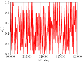
Figure 2: Time evolution of the global parameter $c(r)$ for a given configuration during parallel tempering: data refer to $N=51$, $\beta_{L}=0.6$ and $N_{r}=15$. One MC step corresponds to 4 sweeps of over-relaxation + 1 sweep of over-heatbath; the showed time window corresponds to $0.0025\%$ of the total statistics collected for that run. In this case swap acceptances range from $60\%$ to $20\%$ and are larger for $c(r)$ closer to 1.

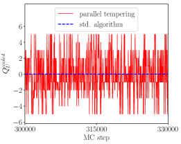
Figure 3: Evolution of $Q_{U}$ after cooling for $N=51$ at $\beta_{L}=0.5$ (above) and $\beta_{L}=0.6$ (below). Results obtained by the Hasenbusch algorithm are compared to the standard algorithm. The horizontal scale corresponds to the same CPU time for the two algorithms and is reported for convenience in MC step units (see caption of Fig. 2). The reported time windows respectively correspond to around $0.013\%$ and $0.0037\%$ of the total statistics collected for the two parallel tempering runs.

The idea put forward in Ref. Hasenbusch (2017), in order to bypass these complications and still take advantage of the improvement of o.b.c., is to consider a collection of similar systems, differing among them for the value of a global parameter which gradually interpolates between o.b.c. and p.b.c.: while each system has an independent Monte Carlo evolution, swap of configurations between different systems are proposed from time to time in a parallel tempering framework. In this way, the fast decorrelation of $Q$ achieved for the open system is progressively transferred to the periodic one, which is also the system where observables are actually measured, thus completely avoiding the complications of open boundaries. The analysis of Ref. Hasenbusch (2017) shows that it suffices to open boundary conditions just along a line defect of length comparable to $\xi_{L}$. Moreover, hierarchical updates around the defect, combined with discrete translations of the periodic system from time to time, helps optimizing the algorithm. For more details, we refer to Ref. Hasenbusch (2017).

The only differences characterizing our implementation are that the algorithm is adapted to the Symanzik-improved action, and that it is used also for simulations at non-zero imaginary $\theta$. Actually, a few preliminary tests showed that the choice of boundary conditions in the $\theta$-term does not affect the efficiency of the algorithm: this is expected, since it is just the usual action term which develops barriers between different topological sectors. Therefore, in order to avoid further complications, we decided to keep periodic boundary conditions in the $\theta$ term for all replicas.

The line defect $D$ was put and held fixed on the time boundary: $D=\{x\,|\,x_{0}=L-1\ \wedge\text{ }0<x_{1}<L_{d}\}$, where $L_{d}$ is the defect length: a geometrical representation is depicted in Fig. 1. Each link crossing the defect line gets multiplied by a factor $c(r)$, where $r$ is the replica index, $r=0,\dots N_{r}-1$. The interpolation between p.b.c.  ($c(r)=1$) and o.b.c. ($c(r)=0$) can be chosen so as to optimize the algorithm, however in practice a simple linear interpolation works already well: $c(r)=1-\frac{r}{N_{r}-1}$. The explicit expression of the lattice action is the following:

$$S_{L}^{(r)}=-2N\beta_{L}\sum_{x,\mu}\left\{k_{\mu}^{(r)}(x)c_{1}\Re\left[\bar{U}_{\mu}(x)\bar{z}(x+\hat{\mu})z(x)\right]\right.\\ \left.+k_{\mu}^{(r)}(x+\hat{\mu})k_{\mu}^{(r)}(x)c_{2}\Re\left[\bar{U}_{\mu}(x+\hat{\mu})\bar{U}_{\mu}(x)\bar{z}(x+2\hat{\mu})z(x)\right]\right\}\,,$$

where

$$k_{\mu}^{(r)}(x)=\begin{cases}c(r)\,,&\quad x\in D\wedge\mu=0\,;\\ 1\,,&\quad\text{otherwise.}\\ \end{cases}$$ (24)

The replica swap was proposed, after every update sweep, for each couple of consecutive replicas, and then accepted according to a Metropolis step with probability:

$$p=\min\left\{1,e^{-\Delta S_{L}}\right\}\,,$$ (25)

where $\Delta S_{L}$ is the global change in the action of the two involved replicas. The length of the defect $L_{d}$ was chosen so that $L_{d}\sim\xi_{L}$ at the highest $\beta_{L}$. Concerning $N_{r}$, for each $N$ we chose it so that, at the highest value of $\beta_{L}$, the lowest acceptance was not lower than $20\%$.

In Fig. 2 we show how a given configuration evolves through different values of $c(r)$ in a typical run. To get the algorithm properly working one should check that swaps happen uniformly, as in the shown example, otherwise the fast decorrelation achieved for o.b.c. is not transferred efficiently across the systems. Finally, in Fig. 3 we compare the MC evolution of $Q$, with and without using parallel tempering, for $N=51$ and for two different values of $\beta_{L}$. Without parallel tempering the charge is almost frozen, while many fluctuations are observed during the same clocktime in the other case, allowing us to perform measures which would have been practically impossible with just the local algorithm.

4 Numerical Results

$N$	$\beta_{L}$	$L$	$\xi_{L}$	$\dfrac{L}{\xi_{L}}$	$\dfrac{L^{2}}{\xi_{L}^{2}N}$	$\theta_{L,\text{{max}}}$	$N_{r}$	$L_{d}$	Stat. $\theta=0$	Stat. $\theta\neq 0$
$21$	0.68	102	4.772(4)	20	20	0	10	6	76M	-
	0.7	114	5.409(4)	21	21	0	11	6	109M	-
$31$	0.54	56	2.218(4)	25	20	6	10	4	12M	10.5M
	0.56	64	2.516(4)	25	20	6	10	4	12M	10.5M
	0.58	72	2.856(5)	25	20	6	10	4	12M	10.5M
	0.6	82	3.239(5)	25	20	6	10	4	16M	21.7M
	0.62	92	3.672(6)	25	20	6	10	4	15M	27.3M
$41$	0.51	58	1.952(3)	29	21	6	13	4	19M	11.2M
	0.53	64	2.213(4)	29	20	6	13	4	17M	11.9M
	0.55	74	2.517(4)	29	21	6	13	4	16M	15.4M
	0.57	82	2.840(5)	29	20	6	13	4	20M	21M
	0.59	92	3.226(5)	28	20	6	13	4	22M	20.3M
	0.61	104	3.655(7)	28	20	6.5	13	4	17M	31.9M
	0.65	132	4.698(6)	28	20	0	15	5	39M	-
$51$	0.5	62	1.902(3)	33	21	6	15	4	17M	11.2M
	0.52	70	2.104(4)	33	22	6	15	4	19M	11.2M
	0.54	78	2.445(4)	32	20	6	15	4	19M	11.9M
	0.56	88	2.779(5)	32	20	6	15	4	18M	11.9M
	0.58	100	3.153(6)	32	20	6.5	15	4	17M	29.7M
	0.6	114	3.560(7)	32	20	6.5	15	4	18M	28.6M

Table 1: Summary of the simulation parameters adopted for all values of $N$. We also report the total accumulated statistics, where each measure was taken after every parallel tempering step. The imaginary-$\theta$ fit was always performed in the range $[0,6]$ with 7 points in steps of $\delta\theta_{L}=1$, except for the $\beta_{L}$ with $\theta_{L,\text{{max}}}=6.5$ where 11 points were taken ($\delta\theta_{L}=1$ up to $\theta_{L}=3$ and then $\delta\theta_{L}=0.5$); $\theta_{L,\text{{max}}}=0$ indicates that no simulation at imaginary $\theta$ has been performed: in this case a single high-statistics run at $\theta=0$ has been used to determine $\chi$ and $\xi$ at the same time. $N_{r}$ indicates the number of replicas used for parallel tempering, the number of hierarchical levels was always 3 (see Hasenbusch (2017) for more details on the hierarchical update).

In Tab. 1 we summarize the parameters and statistics of the simulations performed in the present study, which regarded $N=21,\,31,\,41$ and $51$. In addition, we will also consider results obtained at lower $N$ in previous studies, in order to investigate the large-$N$ behavior of the theory. Results for $N=21$ and $N=31$ have been already reported in Ref. Bonanno et al. (2019), but using lower statistics and/or smaller correlation lengths than in the present work.

Statistics at $\theta_{L}=0$ are generally larger because in this case, apart from the cumulants of the cooled charge $Q_{U}$, we determined the value of the correlation length $\xi_{L}$, which is needed with the best possible precision since it affects the final precision on the continuum extrapolation of $\xi^{2}\chi$. Statistical errors on the cumulants have been estimated by means of a bootstrap analysis.

In the following we will first discuss the impact of finite size effects, in order to justify the choices for the lattice sizes used in our simulations. Then we will illustrate the procedure and discuss the systematics both for the analytic continuation from imaginary $\theta$ and for the extrapolation to the continuum limit of our results; in this respect, we notice that some of our results for $\xi^{2}\chi$ have been produced without relying on analytic continuation (see Tab. 1), in order to provide a robust test that the systematics of analytic continuation and continuum extrapolation are actually under control.

Finally, we will study the large-$N$ expansion of $\xi^{2}\chi$, $b_{2}$, $b_{4}$ based on our and on previous numerical results, illustrating the systematics, the comparison with existing analytic predictions and the estimate of further terms in the expansion.

4.1 Finite size effects

In all of our simulations, and for each fixed value of $N$, we decided to approach the continuum limit keeping the ratio $L/\xi_{L}$ fixed, so as to ensure that the physical volume is kept fixed. In general, taking a ratio $L/\xi_{L}\gg 1$ should ensure that finite size effects be negligible. However, as discussed in Ref. Aguado and Asorey (2011), this is not the case for the $\theta$-dependence of $2d$ $CP^{N-1}$ models in the large-$N$ limit: the large-$N$ limit and the thermodynamic limit do not commute for this class of models, and wrong results might be obtained if the former limit is taken first, leading in practice to the more restrictive condition $(L/\xi_{L})^{2}\gg N$. Since this is strictly related to the particular large-$N$ behavior of the $\theta$-dependence of the theory, we will try to give an intuitive explanation of this condition (see also Ref. Bolognesi et al. (2019) for a related discussion).

Basically, the reason can be traced back to the fact that both $\xi^{2}\chi$ and the $b_{2n}$ coefficients vanish in the large-$N$ limit; indeed, $\xi^{2}\chi$ vanishes as $1/N$, thus, indicating by $l=La$ the size in physical units, one expects for large $N$

$$\langle Q^{2}\rangle=\chi\,l^{2}\simeq\frac{l^{2}}{2\pi\xi^{2}N}\,.$$ (26)

If $l/\xi=L/\xi_{L}$ is kept fixed while $N\to\infty$, one ends up with a system where $\langle Q^{2}\rangle\ll 1$: in these conditions, the distribution of $Q$ is strongly peaked at $Q=0$, with only rare occurences of $Q=\pm 1$ and even rarer occurences of higher values of $|Q|$. It is easy to check that such a distribution leads to $b_{2n}$ coefficients which are very close to those predicted by DIGA, i.e., for instance, $b_{2}=-\langle Q^{4}\rangle_{c}/(12\langle Q^{2}\rangle)\simeq-1/12$. Let us stress that this happens in practice in many other situations, like for instance for 4$d$ Yang-Mills theories in the high-$T$ phase, where $\chi$ vanishes rapidly above $T_{c}$ and one cannot afford to take very large lattice volumes, ending up again with $\langle Q^{2}\rangle\ll 1$; however, in that case the system is really close to DIGA even in the thermodynamical limit, so that, luckily enough, this does not imply significant systematic errors (see Ref. Bonati et al. (2018b) for a thorough discussion about this point).

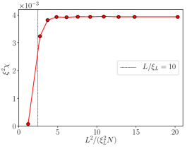
Figure 4: Study of the dependence of $\xi^{2}\chi$ and $b_{2}$ on the lattice size for $N=41$ and $\beta_{L}=0.57$. Lattice sizes range from $L=20$ to $L=82$. Results were obtained by parallel tempering and using the same setup (apart from the lattice size) reported in Tab. 1. The value employed for $\xi_{L}$ is, for all sizes, the one obtained for the largest $L$.

For 2$d$ $CP^{N-1}$ models, instead, the large-$N$ limit is qualitatively different from DIGA, indeed one expects $b_{2}\propto 1/N^{2}$, which is quite different from DIGA predictions. Stated in another way, the particularity of 2$d$ $CP^{N-1}$ models is that while global topological excitations become rarer and rarer as $N\to\infty$, they never become really dilute, as one would naively expect. The additional condition $(L/\xi_{L})^{2}\gg N$ ensures that $\langle Q^{2}\rangle$ is at least of $O(1)$ or larger, so that the non-trivial interactions between topological excitations, which characterize the large-$N$ limit, can be properly taken into account.

$N$	$\beta_{L}$	$\xi_{L}$	$Z$	$a^{2}\chi\cdot 10^{3}$	$\xi^{2}\chi\cdot 10^{3}$	$b_{2}\cdot 10^{3}$	$b_{4}\cdot 10^{6}$	$\tilde{\chi}^{2}$	dof
$21$	0.68	4.772(4)	-	0.3404(6)	7.750(18)	-	-	-	-
	0.7	5.409(4)	-	0.2647(4)	7.746(16)	-	-	-	-
$31$	0.54	2.218(4)	0.876(2)	1.0907(19)	5.365(21)	-2.90(9)	-4.6(1.5)	1.0	17
	0.56	2.517(4)	0.892(2)	0.8353(17)	5.290(22)	-2.67(10)	-1.7(1.6)	0.8	17
	0.58	2.856(5)	0.895(2)	0.6471(17)	5.279(24)	-2.75(12)	-2.8(1.9)	0.7	17
	0.6	3.240(5)	0.903(2)	0.4993(13)	5.240(21)	-2.82(11)	-4.3(1.7)	0.9	17
	0.62	3.672(6)	0.913(3)	0.3876(12)	5.227(23)	-2.59(11)	-2.1(1.7)	1.0	17
$41$	0.51	1.953(3)	0.896(2)	1.0642(16)	4.057(14)	-1.99(8)	-3.5(1.3)	0.9	17
	0.53	2.213(4)	0.903(2)	0.8222(15)	4.027(15)	-1.85(8)	-2.1(1.3)	1.3	17
	0.55	2.517(4)	0.915(2)	0.6295(14)	3.987(17)	-1.84(9)	-2.2(1.4)	0.6	17
	0.57	2.840(5)	0.924(2)	0.4873(11)	3.930(16)	-1.69(9)	-1.1(1.4)	1.2	17
	0.59	3.226(5)	0.928(3)	0.3775(11)	3.930(17)	-1.72(12)	-1.0(1.8)	1.3	17
	0.61	3.655(7)	0.928(3)	0.2936(10)	3.922(20)	-1.76(10)	-2.1(1.3)	1.3	29
	0.65	4.698(6)	-	0.1772(7)	3.912(18)	-	-	-	-
$51$	0.50	1.902(3)	0.917(2)	0.8970(16)	3.244(13)	-1.38(8)	-2.2(1.3)	1.2	17
	0.52	2.104(4)	0.919(2)	0.7297(16)	3.231(14)	-1.55(10)	-4.4(1.5)	1.2	17
	0.54	2.445(4)	0.929(2)	0.5317(13)	3.178(13)	-1.39(11)	-3.4(1.7)	0.9	17
	0.56	2.779(5)	0.932(3)	0.4125(13)	3.186(16)	-1.23(12)	-0.4(2.0)	0.8	17
	0.58	3.153(6)	0.943(3)	0.3172(10)	3.154(16)	-1.27(9)	-1.7(1.1)	1.2	29
	0.60	3.560(7)	0.938(4)	0.2478(10)	3.140(17)	-1.52(18)	-4.2(1.5)	1.7	29

Table 2: Summary of results obtained for $\xi^{2}\chi$, $b_{2}$, $b_{4}$, $Z$ and $\xi_{L}$ for all explored values of $\beta_{L}$ and $N$. All results have been obtained through the imaginary-$\theta$ fit of the first 3 cumulants, except for the two measures at $N=21$ and for the measure at the highest $\beta_{L}$ at $N=41$, where no fit was performed. For all fits we also report the number of dof and the reduced $\tilde{\chi}^{2}$.

In order to illustrate the above considerations in practice, in Fig. 4 we report the behavior of $\xi^{2}\chi$ and $b_{2}$ as a function of the lattice size for $N=41$. It clearly appears that in the small volume limit the system is described by DIGA ($b_{2}\simeq-1/12$), and that finite size corrections are still significant for $L/\xi_{L}=10$. We stress, however, that the range of $L/\xi_{L}$ for which finite size effects are visible at this particular value of $N$ is still compatible with the range observed for other generic (non topological) observables in the same class of models, i.e. $L/\xi_{L}\lesssim 20$ Rossi and Vicari (1993): in order to really observe discrepancies with respect to the indications of Ref. Rossi and Vicari (1993) one should study a case for which $L/\xi_{L}\gtrsim 20$ and $L^{2}/(N\xi_{L}^{2})\lesssim 1$, however that requires $N$ to be of the order of a few hundreds.

In any case, in our simulations we kept $L^{2}/(\xi_{L}^{2}N)\sim 20$ for all explored values of $N$, meaning that $L/\xi_{L}$ depends on $N$ (see Tab. 1). We stress that the condition $L^{2}/(\xi_{L}^{2}N)\gg 1$ was also ensured in the numerical simulations reported in Ref. Bonanno et al. (2019).

4.2 Analytic continuation from imaginary $\theta$ and continuum extrapolation

In Fig. 5 we show an example of the global imaginary-$\theta$ fit discussed in Section 3.2. The best-fit procedure was performed according to Eq. (20) and for just the first 3 cumulants in all cases, exploiting the whole available imaginary $\theta$ range. In order to assess the impact of systematic effects related to analytic continuation, we have tried in each case to change the range fit and the order (i.e. the truncation) of the fit polynomial, verifying that the variation of the fit parameters was within statistical errors, or adding it to the total error otherwise.

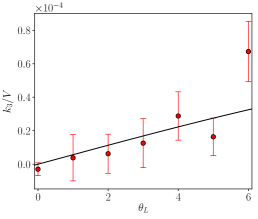
Figure 5: Example of the global imaginary-$\theta$ fit for $N=51$ and $\beta_{L}=0.56$, exploiting the 3 lowest order cumulants and fitting up to $O(\theta_{L}^{6})$ terms. The best fit yields a reduced $\tilde{\chi}^{2}=0.83$ with 17 degrees of freedom (dof).

A complete summary of the results obtained for $Z$, $\xi_{L}$, $\xi^{2}\chi$, $b_{2}$ and $b_{4}$ at all explored values of $N$ and $\beta$ is reported in Tab. 2.

Results collected at different values of $\beta_{L}$ have then been used to obtain continuum extrapolated quantities. In order to discuss the procedure that we have adopted in all cases, we illustrate in details our analysis for the continuum extrapolation of $\xi^{2}\chi$ at $N=21$. Results at finite $\xi_{L}$ are reported in Fig. 6 as a function of $1/\xi_{L}^{2}$, and include both results from Ref. Bonanno et al. (2019) (obtained via analytic continuation) and from this work (obtained just from simulations at $\theta=0$). In general, for the lattice discretization adopted in this work, one expects corrections to the continuum limit for a generic observable $O$, including only the two lowest non-trivial terms, to be as follows:

$$\braket{O}_{L}(\xi_{L})=\braket{O}_{\text{{cont}}}+\frac{A}{\xi_{L}^{2}}+\frac{B}{\xi_{L}^{4}}\,.$$ (27)

In general, for all the quantities considered in this study, a linear extrapolation in $1/\xi_{L}^{2}$, i.e. setting $B=0$, has worked perfectly well, i.e. with reduced $\tilde{\chi}^{2}$ of order 1 for the best fit, in the whole explored range of $\xi_{L}$. However, in order to correctly assess the impact of systematic errors related to the extrapolation, we have also analyzed the effect of including the non-linear term ($B\neq 0$), or of considering the linear fit in a restricted range of $\xi_{L}$, i.e. discarding points which are farther from the continuum limit. The systematics of this procedure are reported in Tab. 3, some of the best fits are reported in Fig. 6 as well. After considering the observed systematics, our final determination for $\xi^{2}\chi$ at $N=21$ has been $\xi^{2}\chi=0.00765(4)$, to be compared with $\xi^{2}\chi=0.00759(5)$ from Ref. Bonanno et al. (2019), $\xi^{2}\chi=0.00767(5)$ from Ref. Hasenbusch (2017) (adopting a different discretization) and $\xi^{2}\chi=0.00800(20)$ from Ref. Del Debbio et al. (2004).

Figure 6: Continuum extrapolation of $\xi^{2}\chi$ for $N=21$. The solid line represents a linear fit in $1/\xi_{L}^{2}$ in the whole range, the dashed line a linear fit on a restricted range and the dotted one a quadratic fit in $1/\xi_{L}^{2}$ in the whole range. Round points represent lattice measures from this study, triangle points are taken from Ref. Bonanno et al. (2019), while the square point is the continuum extrapolated value. Best fit results and the corresponding reduced $\tilde{\chi}^{2}$ values are reported in Tab. 3.

.

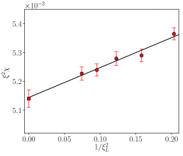
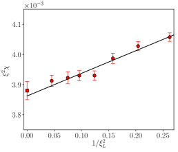
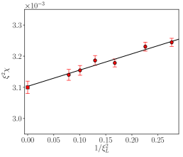
Figure 7: From top to bottom: continuum extrapolations of $\xi^{2}\chi$ for $N=31,\,41$ and $51$. The solid line represents a linear fit in $1/\xi_{L}^{2}$ in the whole range, all best fits yield a reduced $\chi^{2}$ of order 1. Systematics of the continuum extrapolation have been estimated as for $N=21$, the final extrapolated result which is plotted for $1/\xi_{L}^{2}=0$ includes such systematics.

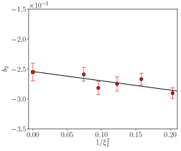
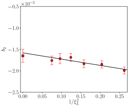
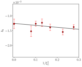
Figure 8: From top to bottom: continuum extrapolations of $b_{2}$ for $N=31,\,41$ and $51$. The solid line represents a linear fit in $1/\xi_{L}^{2}$ in the whole range, all best fits yield a reduced $\chi^{2}$ of order 1. Systematics of the continuum extrapolation have been estimated as for $N=21$, the final extrapolated result which is plotted for $1/\xi_{L}^{2}=0$ includes such systematics.

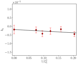
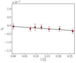
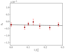
Figure 9: From top to bottom: continuum extrapolations of $b_{4}$ for $N=31,\,41$ and $51$. The solid line represents a linear fit in $1/\xi_{L}^{2}$ in the whole range, all best fits yield a reduced $\chi^{2}$ of order 1. Systematics of the continuum extrapolation have been estimated as for $N=21$, the final extrapolated result which is plotted for $1/\xi_{L}^{2}=0$ includes such systematics.

$\xi_{L,\text{{min}}}$ included	$\xi^{2}\chi\cdot 10^{3}$	$\tilde{\chi}^{2}$	dof
3.07 (quadratic fit)	7.64(6)	1.09	10
3.07 (linear fit)	7.654(21)	0.99	11
3.28	7.636(24)	0.91	9
3.49	7.652(27)	0.88	7
3.72	7.66(3)	1.14	5
3.95	7.66(4)	1.21	3
4.21	7.71(5)	0.10	1

Table 3: Summary of systematics for the continuum extrapolation of $\xi^{2}\chi$ for $N=21$. Our final determination in this case is $\xi^{2}\chi=0.00765(4)$.

The procedure above has been repeated for all explored quantities and for all $N$. In Figs. 7, 8 and 9 we show the continuum extrapolations for $\xi^{2}\chi$, $b_{2}$ and $b_{4}$ for $N=31,41$ and 51, for simplicity of figure reading we report just the linear best fits over the whole range, even if the final continuum determinations take into account the whole systematics, as in the example above.

Final results are shown in Tab. 4, where we report the continuum limit of $\xi^{2}\chi$, $b_{2}$ and $b_{4}$ for $N=21,\,31,\,41$ and $51$, along with continuum results of these observables for other values of $N$ taken from Refs. Bonanno et al. (2019); Hasenbusch (2017).

$N$	$\xi^{2}\chi\cdot 10^{3}$	$b_{2}\cdot 10^{3}$	$b_{4}\cdot 10^{5}$
9	20.00(15)	-13.90(13)	2.04(18)
10	17.37(8)	-	-
11	15.24(12)	-10.7(4)	2.3(5)
13	12.62(9)	-9.1(3)	-0.6(5)
15	10.87(11)	-6.7(3)	0.5(6)
21	7.65(4)	-5.0(5)	-1.7(1.2)
26	6.14(5)	-3.0(4)	-0.3(5)
31	5.14(3)	-2.55(15)	-0.2(3)
41	3.88(3)	-1.65(15)	-0.06(15)
51	3.10(2)	-1.27(16)	-0.24(14)

Table 4: Summary of continuum determinations of $\xi^{2}\chi$, $b_{2}$ and $b_{4}$ for several values of $N$. Results for $N=9,\,11,\,13,\,15$ and $26$, as well as $b_{2}$ and $b_{4}$ for $N=21$, are taken from Ref. Bonanno et al. (2019) while the one for $N=10$ from Ref. Hasenbusch (2017). The result obtained for $\xi^{2}\chi$ at $N=41$ is in good agreement (less than 1$\sigma$) with that obtained using a different discretization in Ref. Hasenbusch (2017) ($\xi^{2}\chi=0.00391(2)$), where however no determination was given for $b_{2}$ and $b_{4}$; for $N=31$ instead one should compare with the results of Ref. Bonanno et al. (2019) ($\xi^{2}\chi=0.00503(6)$, $b_{2}=-0.00231(22)$), also in this case the agreement is reasonable (1.6$\sigma$ and 0.9$\sigma$ respectively).

4.3 Results for $\xi^{2}\chi$ and its large-$N$ scaling

The main purpose of this section is to make use of the results reported in Tab. 4 to investigate the large-$N$ behavior of the topological susceptibility and compare it with analytical predictions. In Fig. 10 we plot the quantity $N\xi^{2}\chi$, which should approach a constant for $N\to\infty$, as a function of $1/N$, together with the LO and NLO analytic computations, and one of our best fits to be discussed in the following.

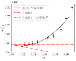
Figure 10: Behavior of $N\xi^{2}\chi$ as a function of $1/N$ compared to LO (dashed line) and NLO (dot-dashed line) analytic computations of the $1/N$ series. The solid line is the result of a best fit to data with $N\geq 10$ where the LO is fixed to the analytic result and the NLO and NNLO are fitted (see Tab. 5 for the complete systematics).

Similarly to what has been done in Ref. Bonanno et al. (2019), we fit our data with a function of the type

$$N\xi^{2}\chi=e_{1}+\frac{e_{2}}{N}+\frac{e_{3}}{N^{2}}+\frac{e_{4}}{N^{3}}$$ (28)

which includes up to N³LO corrections in the $1/N$ expansion: all best-fit systematics are summarized in Tab. 5; in all cases, the LO term has been fixed to the well established analytic prediction $e_{1}=1/(2\pi)$. The systematics for the $e_{2}$ coefficient are also plotted in Fig. 11 in order to make the discussion clearer.

If one sets $e_{3}=e_{4}=0$, thus allowing only for the NLO correction, acceptable or marginally acceptable best fits are obtained when data for $N<13$ are discarded. Nevertheless, results obtained for $e_{2}$ are not stable and show a systematic drift as the fit range is changed, suggesting that NNLO corrections could be important. They are positive and in clear disagreement with the analytic predictions $e_{2}=-0.0605$ Campostrini and Rossi (1991) (as also reported in previous literature) if the fitted range is large enough, but decrease systematically and out-of-the-errors as the fit range is restricted to larger and larger values of $N$, finally becoming negative compatible with the analytic predictions, even if within very large error bars (see Fig. 11).

On the other hand, when the NNLO correction is included in the fit, $e_{3}\neq 0$, results obtained for $e_{2}$ are reasonably stable and compatible with the analytic predictions. Moreover, the NNLO term $e_{3}$ appears quite stable as well, also when the NLO coefficient $e_{2}$ is fixed to the theoretically predicted value, and even when a further term ($e_{4}\neq 0$) is included in the fit, so that we can provide a quite conservative estimate $e_{3}=1.5(5)$, which considers all variations observed for this coefficient in the various fits. The values obtained for $e_{4}$ are not sufficiently precise or stable to allow for any estimate, however we can state it is of $O(10)$.

Finally, we point out that the values obtained for the reduced $\tilde{\chi}^{2}$ for the fits including N²LO and N³LO corrections are generally low: one possible interpretation is that we have been too conservative in estimating the errors on continuum extrapolated quantities, that might also explain why the fit including just $e_{2}$ yields acceptable values of $\tilde{\chi}^{2}$ but is not stable.

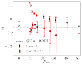
Figure 11: Summary of the fit systematics for the NLO coefficient $e_{2}$ of the $1/N$ expansion of $\xi^{2}\chi$. Empty round points depict determinations of $e_{2}$ from fits with a reduced $\chi^{2}$ with $p$-value smaller than $5\%$ or non existent. The empty diamond point represents our overall estimation: $e_{2}=-0.05(3)$.

Present results clarify why previous lattice studies observed a positive deviations with respect to the LO prediction, in contradiction with the fact that $e_{2}$ is negative: the NNLO term has an opposite sign and, given its estimated magnitude, it is expected to dominate until $N>|e_{3}/e_{2}|\sim 20-30$. Our analysis fully supports the analytic prediction of $e_{2}$. On the other hand, if we had to provide an independent determination of $e_{2}$, a conservative estimate based on our systematics would be $e_{2}=-0.05(3)$, which is still quite inaccurate despite the large numerical effort; the difficulty is clearly related to the fact that $e_{2}$ turns out to be quite small in magnitude, both with respect to $e_{1}$ and $e_{3}$, so that it is hardly detectable.

$N_{\text{{min}}}$	$e_{1}$	$e_{2}$	$e_{3}$	$e_{4}$	$\tilde{\chi}^{2}$	dof
51	$1/(2\pi)$	-0.054(52)			-	0
41	”	-0.028(37)			0.49	1
31	”	-0.007(23)			0.51	2
26	”	-0.001(18)			0.42	3
21	”	0.016(13)			0.71	4
15	”	0.025(12)			1.03	5
13	”	0.039(9)			1.6	6
11	”	0.054(8)			2.8	7
10	”	0.098(6)			11	8
9	”	0.115(5)			15	9
31	$1/(2\pi)$	-0.12(13)	3.9(4.3)		0.21	1
26	”	-0.09(9)	2.8(2.7)		0.16	2
21	”	-0.07(6)	2.2(1.4)		0.13	3
15	”	-0.06(4)	1.8(8)		0.13	4
13	”	-0.042(28)	1.4(5)		0.16	5
11	”	-0.046(24)	1.5(4)		0.15	6
10	”	-0.080(22)	2.2(3)		1.02	7
9	”	-0.093(23)	2.4(3)		1.35	8
41	$1/(2\pi)$	-0.0605	1.8(1.8)		0.36	1
31	”	”	1.9(8)		0.21	2
26	”	”	1.9(6)		0.14	3
21	”	”	1.9(3)		0.11	4
15	”	”	1.9(3)		0.10	5
13	”	”	1.71(15)		0.20	6
11	”	”	1.70(11)		0.17	7
10	”	”	1.9(7)		1.02	8
9	”	”	2.0(6)		1.23	9
11	”	”	2.0(6)	-4(7)	0.14	6
10	”	”	1.3(4)	7(5)	0.9	7
9	”	”	1.0(4)	10(4)	0.92	8

Table 5: Summary of the fit systematics for the determination of the large-$N$ behavior of $\xi^{2}\chi$ using the fit function $N\xi^{2}\chi=e_{1}+e_{2}/N+e_{3}/N^{2}+e_{4}/N^{3}$. Blank spaces mean that the corresponding coefficient was set to 0 in the fit procedure, while numerical values with no error mean that the corresponding coefficient was fixed to that value.

4.4 Large-$N$ scaling for $b_{2}$ and $b_{4}$

We turn now to the analysis of the large-$N$ limit for $b_{2}$. In this case, following again the lines of Ref. Bonanno et al. (2019), we employ a fit function including N³LO corrections

$$N^{2}b_{2}=\bar{b}_{2}+\frac{k_{1}}{N}+\frac{k_{2}}{N^{2}}+\frac{k_{3}}{N^{3}}\,;$$ (29)

that was the minimal polynomial in $1/N$ capable to fit the data available in Ref. Bonanno et al. (2019) after fixing the leading order term to the predicted theoretical value, $\bar{b}_{2}=-27/5$. In Tab. 6 we report systematics for the best-fit procedure, while in Fig. 12 we plot the best fit obtained fitting data to Eq. (29) in the whole available range; the systematics for $\bar{b}_{2}$ are also reported, to improve clarity, in Fig. 13. As it can be appreciated, the new data collected at large $N$ permit us to perform a best fit without fixing the value of the LO term. Results obtained for $\bar{b}_{2}$ are not stable as the fit range is changed if only NLO corrections are included in the fit ($k_{2}=k_{3}=0$), and tend to be more and more compatible with the analytic prediction $\bar{b}_{2}=-5.4$ as the range is restricted to larger and larger values of $N$. When $k_{2}$ and/or $k_{3}$ are included, results for $\bar{b}_{2}$ are more stable and always compatible with the analytic prediction: an independent conservative estimate in this case would be $\bar{b}_{2}=-5(1)$.

Present precision allows also to obtain a rough estimation of the order of magnitude of the corrections to the large-$N$ scaling of $b_{2}$: a conservative estimate for the NLO term, which is sufficiently stable in all performed fits, is $k_{1}=120(60)$. Our results point out that they seem to increase by around one order of magnitude at each step in the expansion, resulting in a very slow convergence towards the large-$N$ limit, as it has already been observed for the topological susceptibility.

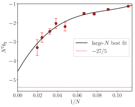
Figure 12: Behavior of $N^{2}b_{2}$ as a function of $1/N$ compared to the LO (dashed line) analytic computation of the $1/N$ series. The solid line is the result of a best fit to data with $N\geq 9$ where all coefficients up to the N³LO are fitted (see Tab. 6 for the complete systematics).

Figure 13: Summary of the fit systematics for the LO coefficient $\bar{b}_{2}$ of the $1/N$ expansion of $b_{2}$. The empty diamond point represents our overall estimation: $\bar{b}_{2}=-5(1)$.

$N_{\text{{min}}}$	$\bar{b}_{2}$	$k_{1}$	$k_{2}$	$k_{3}$	$\tilde{\chi}^{2}$	dof
41	-5.5(2.4)	111(101)			-	0
31	-4.2(8)	55(27)			0.32	1
26	-4.3(7)	58(21)			0.17	2
21	-3.5(4)	32(12)			0.90	3
15	-3.44(21)	29(3)			0.70	4
13	-3.09(18)	21(3)			2.88	5
26	-4.4(2.9)	67(200)	-156(3000)		0.35	1
21	-5.8(1.6)	167(100)	-1901(1300)		0.33	2
15	-4.1(9)	60(40)	-320(400)		0.75	3
13	-4.6(5)	87(19)	-606(180)		0.69	4
11	-3.8(3)	50(10)	-245(80)		1.56	5
9	-3.56(25)	40(6)	-161(40)		1.56	6
15	-7.4(3.0)	329(230)	-7020(6000)	51526(40000)	0.43	2
13	-4.1(1.5)	50(100)	123(1000)	-4434(11000)	0.89	3
11	-5.7(1.1)	159(60)	-2133(1000)	10022(6000)	1.21	4
9	-4.6(6)	92(30)	-939(400)	3521(1900)	1.25	5
41	$-27/5$	108(9)			0.001	1
31	”	94(4)			1.22	2
26	”	93(3)			1.07	3
21	”	84(3)			5.26	4
31	”	147(40)	-1727(1100)		0.15	1
26	”	134(25)	-1256(800)		0.23	2
21	”	144(14)	-1598(400)		0.24	3
15	”	121(6)	-942(100)		1.11	4
13	”	117(5)	-871(60)		1.06	5
11	”	98(3)	-591(40)		5.22	6
26	”	180(110)	-4000(7000)	-50000(100000)	0.27	1
21	”	126(60)	-573(4000)	-13634(40000)	0.32	2
15	”	173(30)	-3254(1300)	23117(13000)	0.44	3
13	”	134(12)	-1467(400)	4959(3500)	0.85	4
11	”	145(9)	-1892(260)	8768(1700)	0.98	5
9	”	132(7)	-1513(150)	6040(800)	1.36	6

Table 6: Summary of the fit systematics for the determination of the large-$N$ behavior of $b_{2}$ using the fit function $N^{2}b_{2}=\bar{b}_{2}+k_{1}/N+k_{2}/N^{2}+k_{3}/N^{3}$. The convention is the same of Tab. 5.

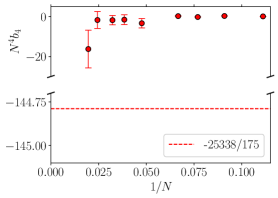
Figure 14: Behavior of $N^{4}b_{4}$ as a function of $1/N$ compared to the LO (dashed line) analytic computation of the $1/N$ series.

Concerning $b_{4}$, so far continuum extrapolated results, which are reported in Fig. 14 in terms of the quantity $N^{4}b_{4}$, are compatible with zero within statistical and systematic uncertainties, so that we can only set upper bounds. Nevertheless, such upper bounds are already interesting enough when compared to LO large-$N$ prediction. Indeed, with present data one would naively set an upper bound on the modulus of the LO order coefficient $|\bar{b}_{4}|\lesssim 20$, which is almost one order of magnitude smaller than the theoretical prediction, $|\bar{b}_{4}|=|-25338/175|\simeq 145$. Therefore, we conclude that large corrections to LO large-$N$ scaling are expected also in the case of $b_{4}$.

5 Conclusions

The main purpose of our study was to clarify the matching between lattice computations and analytic large-$N$ predictions regarding the dependence on the $\theta$-parameter of 2$d$ $CP^{N-1}$ models. The picture emerging from previous lattice studies pointed out to an apparent disagreement for the sign of the deviation of the topological susceptibility from its LO $1/N$ prediction, and to values for the LO $1/N^{2}$ behavior of the $b_{2}$ coefficient missing the predicted analytic value by around a factor 2. A possible way out was proposed in Ref. Bonanno et al. (2019), which showed that assuming large higher order contributions in the $1/N$ expansion, the disagreement could disappear, leading at least to a partial consistency between lattice data and analytic computations. In Ref. Bonanno et al. (2019) it was also pointed out that, assuming the presence of such higher-order corrections, it was necessary to reach at least $N=50$ to make the situation clearer.

In this work we accomplished this goal, exploiting a recent algorithm proposed by M. Hasenbusch to defeat critical slowing down Hasenbusch (2017), which has been adapted to our Symanzik improved discretization in the presence of a $\theta$-term. That allowed us to push our investigation up to $N=51$.

In this way we have been able to provide independent determinations of the NLO and LO coefficients, respectively for $\chi$ and $b_{2}$, which are in agreement with analytic predictions. In particular, we have estimated $e_{2}=-0.05(3)$ (analytic prediction $e_{2}\simeq-0.0605$ Campostrini and Rossi (1991)) and $\bar{b}_{2}=-5(1)$ (analytic prediction $\bar{b}_{2}=-5.4$). At the same time, we have provided a first estimate for the NNLO contribution to $\chi$ ($e_{3}=1.5(5)$) and for the NLO contribution to $b_{2}$ ($k_{1}\sim 120(60)$) which are presently unknown analytically.

Instead, no definite results have been obtained for $b_{4}$, because of the larger statistical uncertainties involved in the determination of this observable, apart from upper bounds which however seem to be in disagreement with the LO large-$N$ prediction by around one order of magnitude, pointing to the presence of large NLO corrections also in this case.

Our results, apart from successfully confirming present analytic estimates for $\chi$ and $b_{2}$, point out that the convergence of the large-$N$ expansion is particularly slow for this class of models. As suggested in Ref. Bonanno et al. (2019), this could be due to the non-analytic behavior which is expected for $N=2$.