Two approaches to the construction of perturbation bounds for continuous-time Markov chains

Abstract. The paper is largely of a review nature. It considers two main methods used to study stability and obtain appropriate quantitative estimates of perturbations of (inhomogeneous) Markov chains with continuous time and a finite or countable state space. An approach is described to the construction of perturbation estimates for the main five classes of such chains associated with queuing models. Several specific models are considered for which the limit characteristics and perturbation bounds for admissible "perturbed"processes are calculated.

Keywords: continuous-time Markov chains, non-stationary Markovian queueing model, stability, perturbation bounds, forward Kolmogorov system.

1 Introduction

In the paper, some topics are considered that are related with the stability of both homogeneous and non-homogeneous continuous-time Markov chains with respect to the perturbation of their intensities (infinitesimal characteristics). It is assumed that the evolution of the system under consideration is described by a Markov chain with the known state space and it is the infinitesimal matrix that is given inexactly. Different classes of admissible perturbations can be considered. The ‘‘perturbed’’ infinitesimal matrix can be arbitrary, and the small deviation of its norm from that of the original matrix is assumed or it can be assumed that the structure of the infinitesimal matrix is known and only its elements are ‘‘perturbed’’ within the same structure. Below we will give a detailed description of these cases. In some papers it is assumed that the perturbations have a special form, for example, are expanded in a power series of a small parameter. This assumption seems to be too restrictive and unrealistic.

The study of stability of characteristics of stochastic models has been actively developing since the 1970-s [19, 43, 71]. At that time V. M. Zolotarev proposed an approach within which limit theorems of probability theory were treated as stability theorems. This approach was cultivated in the works of V. M. Zolotarev, V. V. Kalashnikov, V. M. Kruglov, V. Yu. Korolev and their colleagues in the framework of international seminars on stability problems for stochastic models founded by V. M. Zolotarev (see the series of the proceedings of the seminar published as Springer Lecture Notes starting from [20] or as issues of the Journal of Mathematical Sciences). This approach proved to be very productive for the study of random sums in queueing theory, renewal theory and theory of branching processes [15].

Since 1980-s the problems related to the estimation of stability of Markov chains with respect to perturbations of their characteristics have been thoroughly studied by N. V. Kartashov for homogeneous discrete-time chains with general state space and, in parallel, by A. I. Zeifman for inhomogeneous continuous-time chains within the seminar mentioned above, see [21, 22, 47]. In particular, a general approach for inhomogeneous continuous-time chains was developed in [47]. In that paper both uniform and strong cases were considered. Later birth-death processes were considered in [48] and general properties and estimates for inhomogeneous finite chains were considered in [49]. The paper [51] was specially devoted to estimates for general birth-death processes with the queueing system $M_{t}|M_{t}|N$ considered as an example. It should be mentioned that these papers were not noticed in western papers. For example, in [3] it was stated that there were NO papers on stability of the (simplest stationary!!) system $M|M|1$. For the first time we used the term ‘perturbation bounds’ instead of ‘stability’ in the paper [57] on the referee’s prompt. The same situation takes place with the Kartashov’s papers cited above. The methods proposed in those papers seem to be used by most authors of subsequent studies in estimation of perturbations of discrete-time chains. Possibly, poor acquaintance with the early papers of Kartashov and Zeifman can be explained by the differences in terminology mentioned above: in the original (and foundational) papers the term ’stability’ was used (in the proceedings of the seminar with the consonant appellation ’Stability Problems for Stochastic Models’).

The present paper deals only with continuous-time chains, therefore the subsequent remarks mainly regard such a case.

Note that to obtain explicit and exact estimates of perturbation bounds of a chain, it is required to have estimates of the rate of convergence of the chain to its limit characteristics in the form of explicit inequalities. Moreover, the sharper convergence rate estimates, the more accurate perturbation bounds. These bounds can be more easily obtained for finite homogeneous Markov chains. Therefore, most publications concern just this situation, see, e. g., [2, 7, 30, 31, 32, 33]. As this is so, two main approaches can be highlighted.

The first of them can be used for the case of weak ergodicity of a chain in the uniform operator topology. The first bounds in this direction were obtained in [47]. The principal progress related to the replacement of the constant $S$ with $\log S$ in the bound was implemented in [30] and continued in Mitrophanov’s papers [31, 32, 33] for the case of homogeneous chains and then in [55, 57] and in the subsequent papers of these authors for the inhomogeneous chains. The contemporary state of affairs in this field and new applied problems related to the link between convergence rate and perturbation bounds in the ‘uniform’ case were described in [34]. In some recent papers uniform perturbation bounds of homogeneous Markov chains were studied by the techniques of stochastic differential equations, see for instance [42] and the references therein.

The second approach is used in the case where the uniform ergodicity is not assured, that is typical for the processes most interesting from the practical viewpoint. For example, birth-death processes used for modeling queueing systems, and real processes in biology, chemistry, physics, as a rule, are not uniformly ergodic.

Following the ideas of N. V. Kartashov (see a detailed description in [23]), most authors use the probability methods to study ergodicity and perturbation bounds of stationary chains (with a finite, countable or general state space) in various norms [3, 12, 35]. For a wide class of (mainly) stationary discrete-time chains a close approach was considered in [29] and more recent papers [1, 18, 25, 26, 28, 36, 38, 44, 45, 46, 70].

In the works of the authors of the present paper perturbation bounds for non-stationary finite or infinite continuous-time chains were studied by other methods.

The first papers dealing with non-statonary queueing models appeared in the 1970-s (see [14, 16], and the more recent paper [27]). Moreover, as far back as in [13] it was noted that it is principally possible to use the logarithmic matrix norm for the study of convergence rate of continuous-time Markov chains. The corresponding general approach employing the theory of differential equations in Banach spaces was developed in a series of papers by the authors of the present paper, see a detailed description in [59, 60]. In [47] (also see [48, 49]) a method for the study of perturbation bounds for the vector of state probabilities of a continuous-time Markov chain with respect to the perturbations of infinitesimal characteristics of the chain in the total variation norm ($l_{1}$-norm) was proposed. The paper [51] contained a detailed study of the stability of essentially non-stationary birth-death processes with respect to conditionally small perturbations. Convergence rate estimates in terms of weight norms and hence, the corresponding bounds for new classes of Markov chains were considered in [61, 66, 41, 68].

In the present paper both approaches are considered as well as the classes of inhomogeneous Markov chains for which at least one of these approaches yields reasonable perturbation bounds for basic probability characteristics.

The paper is organized as follows. In Section 2 basic notions and preliminary results are introduced. In Section 3 general theorems on perturbation bounds are considered. Section 4 contains convergence rate estimates and perturbation bounds for basic classes of the chains under consideration. Finally, in Section 5 some special queueing models are studied.

2 Basic notions and preliminaries

Let $X=X(t)$, $t\geq 0$, be, in general, inhomogeneous continuous-time Markov chain with a finite or countable state space $E_{S}=0,1,\dots,S$, $S\leq\infty$. The transition probabilities for $X=X(t)$ will be denoted $p_{ij}(s,t)=\Pr\left\{X(t)=j\left|X(s)=i\right.\right\}$, $i,j\geq 0,\;0\leq s\leq t$. Let $p_{i}(t)=\Pr\left\{X(t)=i\right\}$ be the state probabilities of the chain and ${\bf p}(t)=\left(p_{0}(t),p_{1}(t),\dots\right)^{T}$ be the corresponding vector of state probabilities. In what follows it is assumed that

$$\Pr\left\{X\left(t+h\right)=j|X\left(t\right)=i\right\}=$$

$$=\begin{cases}q_{ij}\left(t\right)h+\alpha_{ij}\left(t,h\right),&\mbox{ if }j\neq i\vspace{1mm}\cr 1-{\displaystyle\sum\limits_{k\neq i}q_{ik}\left(t\right)h+\alpha_{i}\left(t,h\right)},&\mbox{ if }j=i,\end{cases}$$ (1)

where all $\alpha_{i}(t,h)$ are $o(h)$ uniformly in $i$, that is, $\sup_{i}|\alpha_{i}(t,h)|=o(h)$.

As usual, we assume that if a chain is inhomogeneous, then all the infinitesimal characteristics (intensity functions) $q_{ij}\left(t\right)$ are integrable in $t$ on any interval $[a,b]$, $0\leq a\leq b$.

Let $a_{ij}(t)=q_{ji}(t)$ for $j\neq i$ and $a_{ii}(t)=-\sum_{j\neq i}a_{ji}(t)=-\sum_{j\neq i}q_{ij}(t)$.

Further, to provide the possibility to obtain more evident estimates we will assume that

$$|a_{ii}(t)|\leq L<\infty$$ (2)

for almost all $t\geq 0$.

Then the state probabilities satisfy the forward Kolmogorov system

$$\frac{d{\mathbf{p}}}{dt}=A(t){\mathbf{p}}(t),$$ (3)

where $A(t)=Q^{T}(t)$, and $Q(t)$ is the infinitesimal matrix of the process.

Let $\|\cdot\|$ be the usual $l_{1}$-norm, i.e. $\|{{\mathbf{x}}}\|=\sum|x_{i}|$, and $\|B\|=\sup_{j}\sum_{i}|b_{ij}|$ for $B=(b_{ij})_{i,j=0}^{\infty}$. Denote $\Omega=\left\{{{\mathbf{x}}}\,:\,{{\mathbf{x}}}\in l_{1}^{+}\ \&\ \|{{\mathbf{x}}}\|=1\right\}$. Then

$$\|A(t)\|=2\sup_{k}\left|a_{kk}(t)\right|\leq 2L$$

for almost all $t\geq 0$, and we can apply all results of [5] to equation (3) in the space $l_{1}$.

Let $p_{0}(t)=1-\sum_{i\geq 1}p_{i}(t)$. Then from (3) we obtain the following equation (for a detailed discussion, see, e. g., [17, 52]):

$$\frac{d{\mathbf{z}}}{dt}=B(t){\mathbf{z}}(t)+{\mathbf{f}}(t),$$ (4)

where ${\mathbf{f}}(t)=\left(a_{10},a_{20},\cdots\right)^{T}$,

$${B=\left(\begin{array}[]{ccccccccc}a_{11}-a_{10}&a_{12}-a_{10}&\cdots&a_{1r}-a_{10}&\cdots\\ a_{21}-a_{20}&a_{22}-a_{20}&\cdots&a_{2r}-a_{20}&\cdots\\ a_{31}-a_{30}&a_{32}-a_{30}&\cdots&a_{3r}-a_{30}&\cdots\\ \cdots\\ a_{r1}-a_{r0}&a_{r2}-a_{r0}&\cdots&a_{rr}-a_{r0}&\cdots\\ \cdots\cdots\cdots\end{array}\right).}$$ (5)

By $\bar{X}=\bar{X}(t)$ we will denote the ‘perturbed’ Markov chain with the same state space, state probabilities $\bar{p}_{i}(t)$, transposed infinitesimal matrix $\bar{A}(t)=\left(\bar{a}_{ij}(t)\right)_{i,j=0}^{\infty}$ and so on, and the ‘perturbations’ themselves, that is, the differences between the corresponding ‘perturbed’ and original characteristics will be denoted by $\hat{a}_{ij}(t)$, $\hat{A}(t)$.

Let $E(t,k)=E\left\{X(t)\left|X(0)=k\right.\right\}$. Recall that a Markov chain $X(t)$ is weakly ergodic, if $\|{\bf p^{*}}(t)-{\bf p^{**}}(t)\|\to 0$ as $t\to\infty$ for any initial condition, and it has the limiting mean $\phi(t)$, if $|E(t,k)-\phi(t)|\to 0$ as $t\to\infty$ for any $k$.

Now briefly describe the main classes of the chains under consideration. The details concerning the first four classes can be found in [65, 66].

Class I. Let $a_{ij}(t)=0$ for all $t\geq 0$ $|i-j|>1$, $a_{i,i+1}(t)=\mu_{i+1}(t)$, $a_{i+1,i}(t)=\lambda_{i}(t)$. This is an inhomogeneous birth-death process (BDP) with the intensities $\lambda_{i}(t)$ (of birth) and $\mu_{i+1}(t)$ (of death) correspondingly.

Class II. Now let $a_{ij}(t)=0$ for $i<j-1$, $a_{i+k,i}(t)=a_{k}(t)$ for $k\geq 1$, and $a_{i,i+1}(t)=\mu_{i+1}(t)$. This chain describes, for instance, the number of customers in a queueing system in which the customers arrive in groups, but are served one by one (in this case $a_{k}(t)$ is the arrival intensity of a group of $k$ customers, and $\mu_{i}(t)$ is the service intensity of the $i$th customer). The simplest models of this type were considered in [37], also see [65, 66].

Class III. Let $a_{ij}(t)=0$ for $i>j+1$, $a_{i,i+k}(t)=b_{k}(t)$, $k\geq 1$, and $a_{i+1,i}(t)=\lambda_{i}(t)$. This situation occurs in modelling queueing systems with arrivals of single customers and group service.

Class IV. Let $a_{i+k,i}(t)=a_{k}(t)$, $a_{i,i+k}(t)=b_{k}(t)$ for ${k\geq 1}$. This process appears in the description of a system with group arrival and group service, for earlier studies see [39, 40, 61].

Class V. Consider a Markov chain with ‘catastrophes’ used for modelling of some queueing systems, see, e. g., [10, 11, 6, 24, 69, 57]. Here the intensities have a general form whereas a single (although substantial) restriction consists in that the zero state is attainable from any other state and the corresponding intensities $q_{k,0}(t)=a_{0,k}(t)$ for $k\geq 1$ are called the intensities of catastrophes.

Now consider the following example illustrating some specific features of the problem under consideration.

Example [57]. Consider a homogeneous BDP (class I) with the intensities $\lambda_{k}(t)=1$, $\mu_{k}(t)=4$ for all $t$, $k$ and denote by $A$ the corresponding transposed intensity matrix. Then, as is known (see, e. g., [50]), the BDP is strongly ergodic and stable in the corresponding norm. On the other hand, take a perturbed process with the transposed infinitesimal matrix $\bar{A}=A+\hat{A}$, where $\hat{a}_{00}=-\varepsilon$, $\hat{a}_{k0}=\frac{\varepsilon}{k(k+1)}$ for $k\geq 1$ and $\hat{a}_{ij}=0$ for the other $i,j$. Then the perturbed Markov chain $\bar{X}(t)$ (describing the ’M|M|c queue with mass arrivals when empty’, see [4, 24, 69]) is not ergodic, since from the condition $\bar{A}{\bf\bar{p}}=0$ it follows that the coordinates of the stationary distribution (if it exists) must satisfy the condition $4\bar{p}_{k+1}=\bar{p}_{k}+\bar{p}_{0}\frac{\varepsilon}{k+1}\geq\bar{p}_{0}\frac{\varepsilon}{k+1}$, which is impossible.

As it has already been noted, the (upper) bounds of perturbations are closely connected with the (correspondingly, upper) estimates for the convergence rate (also see the two next sections). On the other side, it is also possible to construct important lower estimates of the rate of convergence providing that the influence of the initial conditions cannot fade too rapidly, see [67]. It turns out that it is principally impossible to construct lower bounds for perturbations. Indeed, if we consider the same BDP and as a perturbed BDP choose a BDP with the intensities $\bar{\lambda}_{k}(t)=1+\varepsilon$, $\bar{\mu}_{k}(t)=4(1+\varepsilon)$, then the stationary distribution for the perturbed process will be the same as for the original BDP for any positive $\varepsilon$.

3 General theorems concerning perturbation bounds

First consider uniform bounds.

Theorem 1.

Let the Markov chain $X(t)$ be exponentially weakly ergodic, that is, for any initial conditions ${\bf p^{*}}(s)\in\Omega$, ${\bf p^{**}}(s)\in\Omega$ and any $s\geq 0$, $t\geq s$ there holds the inequality

$$\|{\bf p^{*}}(t)-{\bf p^{**}}(t)\|\leq 2ce^{-b(t-s)}.$$ (6)

Then, for the perturbations small enough ($\hat{A}(t)\leq\varepsilon$ for almost all $t\geq 0$), the perturbed chain $\bar{X}(t)$ is also exponentially weakly ergodic and the following perturbation bound takes place:

$$\limsup_{t\to\infty}\|{\bf p}(t)-{\bar{\bf p}}(t)\|\leq\frac{\left(1+\log(c/2)\right)\varepsilon}{b}.$$ (7)

For the proof we will use the approach proposed in [30] and modified in [55] for the inhomogeneous case, also see [57]. Let

$$\beta(t,s)=\sup_{\|{\bf v}\|=1,\sum{v_{i}}=0}{\|U(t){\bf v}\|}={\textstyle\frac{1}{2}}\sup_{i,j}\sum_{k}{|p_{ik}(t,s)-p_{jk}(t,s)|}.$$ (8)

Then

$$\|{\bf p}(t)-{\bf\bar{p}}(t)\|\leq\beta(t,s)\|{\bf p}(s)-{\bf\bar{p}}(s)\|+\int_{s}^{t}\|\hat{A}(u)\|\beta(u,s)du,$$ (9)

moreover,

$$\beta(t,s)\leq 1,\quad\beta(t,s)\leq{\textstyle\frac{c}{2}}e^{-b(t-s)},\ 0\leq s\leq t.$$ (10)

$$\|{\bf p}(t)-\bar{\bf p}(t)\|\leq$$

$$=\begin{cases}\|{\bf p}(s)-{\bf\bar{p}}(s)\|+(t-s)\varepsilon,&0<t\!-\!s<{\textstyle\frac{1}{b}}\ln{\frac{c}{2}},\vspace{1mm}\cr{\frac{c}{2}e^{-b(t-s)}\|{\bf p}(s)-{\bf\bar{p}}(s)\|\!+\!\textstyle\frac{1}{b}}(\ln{\frac{c}{2}}\!+1\!-\!ce^{-b(t-s)})\varepsilon,&t\!-\!s\geq{\textstyle\frac{1}{b}}\ln{\frac{c}{2}},\end{cases}$$ (11)

whence, as $t\to\infty$, we obtain (7).

Corollary 1.

If under the conditions of theorem 1 the Markov chain $X(t)$ has a finite state space, then both Markov chains $X(t)$ and $\bar{X}(t)$ have limit expectations and

$$|\phi(t)-\bar{\phi}(t)|\leq{\textstyle\frac{1}{b}}S\left(1+\log(c/2)\right)\varepsilon.$$ (12)

Now turn to the weighted bounds. Here we use the approach proposed in [47], also see the detailed description in [59, 60].

Let $1\leq d_{1}\leq d_{2}\leq\dots$,

$$D=\left(\begin{array}[]{ccccccc}d_{1}&d_{1}&d_{1}&\cdots\\ 0&d_{2}&d_{2}&\cdots\\ 0&0&d_{3}&\cdots\\ &\ddots&\ddots&\ddots\\ \end{array}\right).$$ (13)

Let $l_{1D}=\left\{{\bf z}=(p_{1},p_{2},\cdots)^{T}\,:\,\|{\bf z}\|_{1D}\equiv\|D{\bf z}\|<\infty\right\}$. Then $\|B\|_{1D}=\|DBD^{-1}\|$. In addition, let $\|{\bf p}\|_{1D}=\|{\bf z}\|_{1D}$.

Below we will assume that the following conditions hold:

$$\|B(t)\|_{1D}\leq\mathfrak{B}<\infty,\quad\|{\bf f}(t)\|_{1D}\leq\mathfrak{f}<\infty$$ (14)

for almost all $t\geq 0$.

Recall that $X(t)$ is $1D$-exponentially weakly ergodic Markov chain, if

$$\|{\bf p^{*}}(t)-{\bf p^{**}}(t)\|_{1D}\leq Me^{-a\left(t-s\right)}\|{\bf p^{*}}(s)-{\bf p^{**}}(s)\|_{1D}.$$ (15)

for some $M>0$, $a>0$ and any $s,t$: $t\geq s\geq 0$, any initial conditions ${\bf p^{*}}(s)\in l_{1D}$, ${\bf p^{**}}(s)\in l_{1D}$.

If one can choose ${\bf p^{**}}(t)={\bf\pi}$, then the chain is $1D$-exponentially strongly ergodic.

Let

$$\|B(t)-\bar{B}(t)\|_{1D}\leq\left|\mathfrak{B-\bar{B}}\right|,\quad\|{\bf f}(t)-\bar{{\bf f}}(t)\|_{1D}\leq\left|\mathfrak{f-\bar{f}}\right|.$$ (16)

for almost all $t\geq 0$.

Theorem 2.

If a Markov chain $X(t)$ is $1D$-exponentially weakly ergodic, then $\bar{X}(t)$ is also $1D$-exponentially weakly ergodic and the following perturbation estimate in the $1D$-norm holds:

$$\limsup_{t\to\infty}\|{\bf p}(t)-{\bar{\bf p}}(t)\|_{1D}\leq\frac{M\left(M\left|\mathfrak{B-\bar{B}}\right|\mathfrak{f}+a\left|\mathfrak{f-\bar{f}}\right|\right)}{a\left(a-M\left|\mathfrak{B-\bar{B}}\right|\right)}.$$ (17)

If $W=\inf_{i\geq 1}\frac{d_{i}}{i}>0$, then both chains $X(t)$ and $\bar{X}(t)$ have limiting means and

$$\limsup_{t\to\infty}|\phi(t)-\bar{\phi}(t)|\leq\frac{M\left(M\left|\mathfrak{B-\bar{B}}\right|\mathfrak{f}+a\left|\mathfrak{f-\bar{f}}\right|\right)}{Wa\left(a-M\left|\mathfrak{B-\bar{B}}\right|\right)}.$$ (18)

Proof..

The detailed consideration can be found in [60]. Here we only outline the scheme of reasoning. Let $V(t,s)$ and $\bar{V}(t,s)$ be the Cauchy operators for equation (4) and for the corresponding ’perturbed’ equation, respectively. Then

$$\|V(t,s)\|_{1D}\leq Me^{-a(t-s)},\quad\|\bar{V}(t,s)\|_{1D}\leq Me^{-\left(a-M\left|\mathfrak{B-\bar{B}}\right|\right)(t-s)}$$ (19)

for all $t\geq s\geq 0$. Then, rewriting equation (4) as

$$\frac{d{\mathbf{z}}}{dt}=\bar{B}(t){\mathbf{z}}(t)+{\bf f}(t)+\left(B(t)-\bar{B}(t)\right){\mathbf{z}}(t),$$ (20)

after some algebra we obtain the following inequality in the $1D$-norm:

$$\left\|{\mathbf{z}}(t)-\bar{{\mathbf{z}}}(t)\right\|\leq\int_{0}^{t}\|\bar{V}(t,\tau)\|\left(\|B(\tau)-\bar{B}(\tau)\|\|{\mathbf{z}}(\tau)\|+\|{\mathbf{f}}(\tau)-\bar{{\mathbf{f}}}(\tau)\|\right)\ d\tau\leq$$

$$\leq\int_{0}^{t}Me^{-\left(a-M\left|\mathfrak{B-\bar{B}}\right|\right)(t-\tau)}\left(\left|\mathfrak{B-\bar{B}}\right|\|{\mathbf{z}}(\tau)\|+\left|\mathfrak{f-\bar{f}}\right|\right)\ d\tau.$$ (21)

On the other hand, $\|{\mathbf{z}}(t)\|_{1D}\leq Me^{-at}\|{\mathbf{z}}(0)\|_{1D}+\frac{M}{a}\mathfrak{f}$, for any $0\leq s\leq t$. Hence, under any initial condition ${\mathbf{z}}(0)\in l_{1D}$ we obtain the following inequalities for the $1D$-norm:

$$\left\|{\mathbf{z}}(t)-\bar{{\mathbf{z}}}(t)\right\|\leq M\left(\left|\mathfrak{B-\bar{B}}\right|\frac{M}{a}\mathfrak{f}+\left|\mathfrak{f-\bar{f}}\right|\right)\int_{0}^{t}e^{-\left(a-M\left|\mathfrak{B-\bar{B}}\right|\right)(t-\tau)}\,d\tau+$$

$$+M\int_{0}^{t}e^{-\left(a-M\left|\mathfrak{B-\bar{B}}\right|\right)(t-\tau)}\left|\mathfrak{B-\bar{B}}\right|Me^{-a\tau}\|{\mathbf{z}}(0)\|\,d\tau\leq$$

$$\leq\frac{M\left(M\left|\mathfrak{B-\bar{B}}\right|\mathfrak{f}+a\left|\mathfrak{f-\bar{f}}\right|\right)}{a\left(a-M\left|\mathfrak{B-\bar{B}}\right|\right)}+o\left(1\right).$$ (22)

So, the first assertion of the theorem is proved.

Then second assertion follows from the inequality $\|{\mathbf{z}}\|_{1E}\leq W^{-1}\|{\mathbf{z}}\|_{1D}$ (see, e. g., [52]) and estimate (22), where $l_{1E}=\left\{z=(p_{1},p_{2},\ldots)^{T}\,:\,\|z\|_{1E}\equiv\sum n|p_{n}|<\infty\right\}$. ∎

Remark 1.

A number of consequences of this statement can be formulated, for example,

$$\limsup_{t\to\infty}\|{\bf p}(t)-{\bar{\bf p}}(t)\|\leq\frac{4M\left(M\left|\mathfrak{B-\bar{B}}\right|\mathfrak{f}+a\left|\mathfrak{f-\bar{f}}\right|\right)}{ad\left(a-M\left|\mathfrak{B-\bar{B}}\right|\right)},$$ (23)

this follows from

$$\|{\mathbf{p}}^{*}-{\mathbf{p}}^{**}\|\leq 2\|{\mathbf{z}}^{*}-{\mathbf{z}}^{**}\|\leq\frac{4}{d}\|{\mathbf{z}}^{*}-{\mathbf{z}}^{**}\|_{1D}.$$ (24)

The respective perturbation bounds can be formulated for strongly ergodic (for instance, homogeneous) Markov chains, see [60].

Remark 2.

As it was shown in [60], the bounds presented in theorem 2 and its corollaries are sufficiently sharp.

4 Convergence rate estimates and perturbation bounds for main classes

For Markov chains of classes I – IV an important role is played by the matrix $B^{**}(t)=DB(t)D^{-1}$. To begin with, write out this matrix for each of these classes.

For class I this matrix has the form

$B^{**}(t)=$

$${=\!\footnotesize\left(\!\begin{array}[]{ccccccc}-\left(\lambda_{0}\!+\!\mu_{1}\right)&\frac{d_{1}}{d_{2}}\mu_{1}&0&\cdots&0&\cdots&\cdots\vspace{1mm}\\ \frac{d_{2}}{d_{1}}\lambda_{1}&-\!\left(\lambda_{1}\!+\!\mu_{2}\right)&\frac{d_{2}}{d_{3}}\mu_{2}&\cdots&0&\cdots&\cdots\vspace{1mm}\\ \ddots&\ddots&\ddots&\ddots&\ddots&\cdots\vspace{1mm}\\ 0&\cdots&\cdots&\frac{d_{r}}{d_{r-1}}\lambda_{r-1}&-\!\left(\lambda_{r-1}\!+\!\mu_{r}\right)&\frac{d_{r}}{d_{r+1}}\mu_{r}&\cdots\vspace{1mm}\\ \cdots&\cdots&\cdots&\cdots&\cdots&\cdots&\cdots\\ \end{array}\!\right)}$$ (25)

in the case of a countable state space ($S=\infty$);

$B^{**}(t)=$

$$=\!{\left(\!\begin{array}[]{ccccc}-\left(\lambda_{0}\!+\!\mu_{1}\right)&\frac{d_{1}}{d_{2}}\mu_{1}&0&\cdots&0\vspace{1mm}\\ \frac{d_{2}}{d_{1}}\lambda_{1}&-\!\left(\lambda_{1}\!+\!\mu_{2}\right)&\frac{d_{2}}{d_{3}}\mu_{2}&\cdots&0\vspace{1mm}\\ \ddots&\ddots&\ddots&\ddots&\ddots\vspace{1mm}\\ 0&\cdots&\cdots&\frac{d_{S}}{d_{S-1}}\lambda_{S-1}&-\!\left(\lambda_{S-1}\!+\!\mu_{S}\right)\end{array}\!\right)}$$ (26)

in the case of a finite state space ($S<\infty$).

For class II this matrix has the form

$${B^{**}(t)=\left(\begin{array}[]{cccccc}a_{11}&\frac{d_{1}}{d_{2}}\mu_{1}&0&\cdots&0\vspace{1mm}\\ \frac{d_{2}}{d_{1}}a_{1}&a_{22}&\frac{d_{2}}{d_{3}}\mu_{2}&\cdots&0\vspace{1mm}\\ \frac{d_{3}}{d_{1}}a_{2}&\frac{d_{3}}{d_{2}}a_{1}&a_{33}&\frac{d_{3}}{d_{4}}\mu_{3}&\cdots&\vspace{1mm}\hfil\\ \ddots&\ddots&\ddots&\ddots&\ddots\vspace{1mm}\\ \ddots&\ddots&\ddots&\ddots&\ddots\vspace{1mm}\\ \end{array}\right)}$$ (27)

in the case of a countable state space ($S=\infty$);

$B^{**}(t)=$

$$={\left(\begin{array}[]{ccccc}a_{11}-a_{S}&\frac{d_{1}}{d_{2}}\mu_{1}&0&\cdots&0\vspace{1mm}\\ \frac{d_{2}}{d_{1}}\left(a_{1}-a_{S}\right)&a_{22}-a_{S-1}&\frac{d_{2}}{d_{3}}\mu_{2}&\cdots&0\vspace{1mm}\\ \ddots&\ddots&\ddots&\ddots&\ddots\vspace{1mm}\\ \frac{d_{S}}{d_{1}}\left(a_{S-1}-a_{S}\right)&\cdots&\cdots&\frac{d_{S}}{d_{S}-1}\left(a_{1}-a_{2}\right)&a_{SS}-a_{1}\end{array}\right)}$$ (28)

in the case of a finite state space ($S<\infty$).

For class III this matrix has the form

$B^{**}(t)=$

$$=\!{\footnotesize\left(\!\begin{array}[]{cccccc}-\left(\lambda_{0}\!+\!b_{1}\right)&\frac{d_{1}}{d_{2}}\left(b_{1}\!-\!b_{2}\right)&\frac{d_{1}}{d_{3}}\left(b_{2}\!-\!b_{3}\right)&\cdots&\cdots\vspace{1mm}\\ \frac{d_{2}}{d_{1}}\lambda_{1}&-\big{(}\lambda_{1}\!+\!\sum\limits_{i\leq 2}b_{i}\big{)}&\frac{d_{2}}{d_{3}}\left(b_{1}\!-\!b_{3}\right)&\cdots&\cdots\vspace{1mm}\\ \ddots&\ddots&\ddots&\ddots&\ddots\vspace{1mm}\\ 0&\cdots&\cdots&\frac{d_{r}}{d_{r-1}}\lambda_{r-1}&-\big{(}\lambda_{r-1}\!+\!\sum\limits_{i\leq r}b_{i}\big{)}\cdots\vspace{1mm}\\ \ddots&\ddots&\ddots&\ddots&\ddots\vspace{1mm}\\ \end{array}\!\right)}$$ (29)

in the case of a countable state space ($S=\infty$);

$B^{**}(t)=$

$$=\!{\footnotesize\left(\!\begin{array}[]{ccccc}-\!\left(\lambda_{0}\!+\!b_{1}\right)&\frac{d_{1}}{d_{2}}\left(b_{1}\!-\!b_{2}\right)&\frac{d_{1}}{d_{3}}\left(b_{2}\!-\!b_{3}\right)&\cdots&\frac{d_{1}}{d_{S}}\left(b_{S-1}\!-\!b_{S}\right)\vspace{1mm}\\ \frac{d_{2}}{d_{1}}\lambda_{1}&-\!\big{(}\lambda_{1}\!+\!\sum\limits_{i\leq 2}b_{i}\big{)}&\frac{d_{2}}{d_{3}}\left(b_{1}\!-\!b_{3}\right)&\cdots&\frac{d_{2}}{d_{S}}\left(b_{S-2}\!-\!b_{S}\right)\vspace{1mm}\\ \ddots&\ddots&\ddots&\ddots&\ddots\vspace{1mm}\\ 0&\cdots&\cdots&\frac{d_{S}}{d_{S-1}}\lambda_{S-1}&-\!\big{(}\lambda_{S-1}\!+\!\sum\limits_{i\leq S}b_{i}\big{)}\end{array}\right)}$$ (30)

in the case of a finite state space ($S<\infty$).

Finally, for class IV this matrix has the form

$$B^{**}={\left(\begin{array}[]{cccccc}a_{11}&\frac{d_{1}}{d_{2}}\left(b_{1}-b_{2}\right)&\frac{d_{1}}{d_{3}}\left(b_{2}-b_{3}\right)&\cdots&\cdots\vspace{1mm}\\ \frac{d_{2}}{d_{1}}a_{1}&a_{22}&\frac{d_{2}}{d_{3}}\left(b_{1}-b_{3}\right)&\cdots&\cdots\vspace{1mm}\\ \ddots&\ddots&\ddots&\ddots&\ddots\vspace{1mm}\\ \frac{d_{r}}{d_{1}}a_{r-1}&\cdots&\cdots&\frac{d_{r}}{d_{r-1}}a_{1}&a_{rr}&\cdots\vspace{1mm}\\ \cdots&\cdots&\cdots&\cdots&\cdots&\cdots\\ \end{array}\right)}$$ (31)

in the case of a countable state space ($S=\infty$);

$B^{**}(t)=$

$$=\!{\footnotesize\left(\!\begin{array}[]{ccccc}a_{11}\!-\!a_{S}&\frac{d_{1}}{d_{2}}\left(b_{1}\!-\!b_{2}\right)&\frac{d_{1}}{d_{3}}\left(b_{2}\!-\!b_{3}\right)&\cdots&\frac{d_{1}}{d_{S}}\left(b_{S-1}\!-\!b_{S}\right)\vspace{1mm}\\ \frac{d_{2}}{d_{1}}\left(a_{1}\!-\!a_{S}\right)&a_{22}\!-\!a_{S-1}&\frac{d_{2}}{d_{3}}\left(b_{1}\!-\!b_{3}\right)&\cdots&\frac{d_{2}}{d_{S}}\left(b_{S-2}\!-\!b_{S}\right)\vspace{1mm}\\ \ddots&\ddots&\ddots&\ddots&\ddots\vspace{1mm}\\ \frac{d_{S}}{d_{1}}\left(a_{S-1}\!-\!a_{S}\right)&\cdots&\cdots&\frac{d_{S}}{d_{S-1}}\left(a_{1}\!-\!a_{2}\right)&a_{SS}\!-\!a_{1}\end{array}\!\right)}$$ (32)

in the case of a finite state space ($S<\infty$).

In the proofs of the following theorems we use the notion of the logarithmic norm of a linear operator function and related estimates of the norm of the Cauchy operator of a linear differential equation. The corresponding results were described in detail in our preceding works, see [17, 52, 66]. Here we restrict ourselves only to the necessary minimum.

Recall that the logarithmic norm of an operator function ${B^{**}}(t)$ is defined as the number

$$\gamma({B^{**}}(t))=\lim_{h\to+0}h^{-1}\left(\|I+hB^{**}(t)\|-1\right).$$

Let $V(t,s)=V(t)V^{-1}(s)$ be the Cauchy operator of the differential equation

$$\frac{d{\bf w}}{dt}={B^{**}}(t){\bf w}.$$

Then the estimate

$$\|V(t,s)\|\leq e^{\,\int_{s}^{t}\gamma(B^{**}(u))\,du}$$

holds. Moreover, if for each $t\geq 0$ $B^{**}(t)$ maps $l_{1}$ into itself, then the logarithmic norm can be calculated by the formula

$$\gamma({B^{**}}(t))=\sup_{1\leq j\leq S}\left(b_{jj}^{**}(t)+\sum_{i\neq j}|b_{ij}^{**}(t)|\right).$$ (33)

Now let

$$\alpha_{i}\left(t\right)=-\left(b_{jj}^{**}(t)+\sum_{i\neq j}|b_{ij}^{**}(t)|\right),\ \alpha\left(t\right)=\inf_{i\geq 1}\alpha_{i}\left(t\right).$$ (34)

Also note that if in classes II–IV the intensities $a_{k}(t)$ and $b_{k}(t)$ do not increase in $k$ for each $t$, then in all the cases the matrix ${B^{**}}(t)$ is essentially nonnegative (that is, its non-diagonal elements are nonnegative), then in (33) and (34) the signs of the absolute value can be omitted.

The following statement ([66, theorem 1]) is given here for convenience.

Theorem 3.

Let for some sequence $\{d_{i},\ i\geq 1\}$ of positive numbers the conditions $d_{1}=1$, $d=\inf_{i\geq 1}d_{i}>0$ and

$$\int_{0}^{\infty}\alpha(t)\,dt=+\infty$$ (35)

hold. Then the Markov chain $X(t)$ is weakly ergodic and for any initial condition $s\geq 0$, ${\bf w}(s)$ and for all $t\geq s$ there holds the estimate

$$\|{\bf w}\left(t\right)\|\leq e^{-\int_{s}^{t}{\alpha\left(u\right)du}}\|{\bf w}(s)\|.$$ (36)

Now let instead of (35), for all $0\leq s\leq t$ a stronger condition

$$e^{-\int_{s}^{t}\alpha(\tau)\,d\tau}\leq M^{*}e^{-a^{*}(t-s)}$$ (37)

holds.

Theorem 4.

Let under the conditions of theorem 3 inequality (37) holds. Then the Markov chain $X(t)$ is $1D$-exponentially weakly ergodic and for all $t\geq s\geq 0$ and ${\bf p^{*}}(s)\in l_{1D}$, ${\bf p^{**}}(s)\in l_{1D}$ there holds the inequality (15) with $M=M^{*}$ and $a=a^{*}$.

Remark 3.

In the case of a homogeneous Markov chain or if all intensities are periodic with one and the same period, conditions (35) and (37) are equivalent.

Theorem 5.

Let the conditions of theorem 4 hold. Then the Markov chain $X(t)$ is $1D$-exponentially weakly ergodic, under perturbations small enough (16) the perturbed chain $\bar{X}(t)$ is also $1D$-exponentially weakly ergodic and perturbation bound (38) in the $1D$-norm holds. If, moreover, $W=\inf_{i\geq 1}\frac{d_{i}}{i}>0$, then both chains $X(t)$ and $\bar{X}(t)$ have limit expectations and estimate (18) holds for the perturbation of the mathematical expectation.

To obtain perturbation bounds in the natural norm it suffices to use inequality (24) mentioned above.

Corollary 2.

Under the conditions of theorem 5 the following perturbation bound in the natural $l_{1}$- (total variation) norm holds:

$$\limsup_{t\to\infty}\|{\bf p}(t)-{\bar{\bf p}}(t)\|\leq\frac{4M\left(M\left|\mathfrak{B-\bar{B}}\right|\mathfrak{f}+a\left|\mathfrak{f-\bar{f}}\right|\right)}{ad\left(a-M\left|\mathfrak{B-\bar{B}}\right|\right)}.$$ (38)

Note that it is convenient to use the results formulated above for the construction of perturbation bounds for Markov chains of the first four classes, see, e. g., [51, 60, 61, 66].

For chains of the fifth class, as a rule, it is convenient to use the approach based on uniform bounds as will be shown below. These models were considered, e. g., in [57, 62, 63].

Let

$$\beta_{*}\left(t\right)=\inf_{k}a_{0k}(t).$$ (39)

Theorem 6.

Let the intensities of catastrophes be essential, that is

$$\int_{0}^{\infty}\beta_{*}\left(t\right)\,dt=+\infty.$$ (40)

Then the chain $X\left(t\right)$ is weakly ergodic in the uniform operator topology and for any initial conditions ${{\bf p}}^{*}\left(0\right),{{\bf p}}^{**}\left(0\right)$ and any $0\leq s\leq t$ there holds the following convergence rate estimate:

$$\left\|{{\bf p}}^{*}\left(t\right)-{{\bf p}}^{**}\left(t\right)\right\|\leq 2e^{-\int\limits_{s}^{t}\beta_{*}\left(\tau\right)\,d\tau}.$$ (41)

To prove this theorem we will use the same technique as in [57]. Rewrite the direct Kolmogorov system (3) in the form

$$\frac{d{\bf p}}{dt}=A^{*}\left(t\right){{\bf p}}+{\bf g}\left(t\right),\quad t\geq 0.$$ (42)

Here ${\bf g}\left(t\right)=\left(\beta_{*}\left(t\right),0,0,\dots\right)^{T}$, $A^{*}\left(t\right)=\left(a_{ij}^{*}\left(t\right)\right)_{i,j=0}^{\infty}$, and

$$a_{ij}^{*}\left(t\right)=\begin{cases}a_{0j}\left(t\right)-\beta_{*}\left(t\right),&\mbox{ if }i=0,\vspace{1mm}\cr a_{ij}\left(t\right),&\mbox{ otherwise }.\end{cases}$$ (43)

The solution to this equation can be written as

$${\bf p}\left(t\right)=U^{*}\left(t,0\right){\bf p}\left(0\right)+\int_{0}^{t}{}U^{*}\left(t,\tau\right){\bf g}\left(\tau\right)\,d\tau,$$ (44)

where $U^{*}\left(t,s\right)$ is the Cauchy operator of the differential equation

$$\frac{d{\bf z}}{dt}=A^{*}\left(t\right){{\bf z}}.$$ (45)

Note that the matrix $A^{*}\left(t\right)$ is essentially nonnegative for all $t\geq 0$. Its logarithmic norm is equal to

$$\gamma(A^{*}(t))=\sup_{i}\left(a_{ii}^{*}\left(t\right)+\sum_{j\neq i}a_{ji}^{*}\left(t\right)\right)=-\beta_{*}\left(t\right),$$ (46)

and hence,

$$\left\|{{\bf p}}^{*}\left(t\right)-{{\bf p}}^{**}\left(t\right)\right\|\leq e^{-\int\limits_{s}^{t}\beta_{*}\left(\tau\right)\,d\tau}\left\|{{\bf p}}^{*}\left(s\right)-{{\bf p}}^{**}\left(s\right)\right\|\leq 2e^{-\int\limits_{s}^{t}\beta_{*}\left(\tau\right)\,d\tau}.$$ (47)

Theorem 7.

Let, instead of (40), the stronger condition

$$e^{-\int_{s}^{t}\beta_{*}(\tau)\,d\tau}\leq c^{*}e^{-b^{*}(t-s)}$$ (48)

hold. Then the chain $X\left(t\right)$ is weakly exponentially ergodic in the uniform operator topology, and if the perturbations are small enough, that is, $\|\hat{A}(t)\|\leq\varepsilon$ for almost all $t\geq 0$, then the perturbed chain $\bar{X}(t)$ is also exponentially weakly ergodic and the perturbation bound (7) holds with $c=c^{*}$, $b=b^{*}$.

5 Examples

First of all note that many examples of perturbation bounds for queueing systems were considered in [49, 51, 54, 56, 57, 61, 60].

Here, to compare both approaches, we will mostly deal with the queueing system $M_{t}|M_{t}|N|N$ with losses and $1$-periodic intensities. In the preceding papers on this model, other problems were considered. For example, in [8] the asymptotics of the rate of convergence to the stationary mode as $N\to\infty$, was studied, whereas the paper [9] dealt with the asymptotics of the convergence parameter under various limit relations between the intensities and the dimensionality of the model. In [54, 56] perturbation bounds were considered under additional assumptions.

Let $N\geq 1$ be the number of servers in the system. Assume that the customers arrival intensity $\lambda(t)$ and the service intensity of a server $\mu(t)$ are $1$-periodic nonnegative functions integrable on the interval $[0,1]$. Then the number of customers in the system (queue length) $X(t)$ is a finite Markov chain of class I, that is, a BDP with the intensities $\lambda_{k-1}(t)=\lambda(t)$, $\mu_{k}(t)=k\mu(t)$ for $k=1,\dots,N$.

It should be especially noted that the process $X(t)$ is weakly ergodic (obviously, exponentially and uniformly ergodic, since the intensities are periodic and the state space is finite), if and only if

$$\int_{0}^{1}\left(\lambda(t)+\mu(t)\right)\,dt>0,$$ (49)

see, e. g., [53].

For definiteness, assume that $\int_{0}^{1}\mu(t)\,dt>0.$

Apply the approach described in theorems 3 and 4.

Let all $d_{k}=1$. Then

$$B^{**}(t)={\left(\begin{array}[]{ccccc}-\left(\lambda+\mu\right)&\mu&0&\cdots&0\\ \lambda&-\left(\lambda+2\mu\right)&2\mu&\cdots&0\\ \ddots&\ddots&\ddots&\ddots&\ddots\\ 0&\cdots&\cdots&\lambda&-\left(\lambda+N\mu\right)\end{array}\right),}$$ (50)

and in (34) we have $\alpha_{i}\left(t\right)=\mu(t)$ for all $i$, hence, $\alpha\left(t\right)=\mu(t)$.

Therefore, theorem 3 yields the estimate

$$\|{\bf p^{*}}(t)-{\bf p^{**}}(t)\|_{1D}\leq e^{-\int_{s}^{t}\mu(\tau)\,d\tau}\|{\bf p^{*}}(s)-{\bf p^{**}}(s)\|_{1D}.$$ (51)

To find the constants in the estimates, let $\mu^{*}=\int_{0}^{1}\mu(\tau)\,d\tau$ and consider

$$\int_{0}^{t}\mu(\tau)\,d\tau=\mu^{*}t+\int_{0}^{\{t\}}\left(\mu(\tau)-\mu^{*}\right)\,d\tau.$$ (52)

Find the bound for the second summand in (52). Assuming $u=\{t\}$, we obtain

$$\left|\int_{0}^{u}\left(\mu(\tau)-\mu^{*}\right)\,d\tau\right|\leq K^{*}=\sup_{u\in[0,1]}\int_{0}^{u}\left(\mu(\tau)-\mu^{*}\right)\,d\tau.$$ (53)

Then

$$e^{-\int_{s}^{t}\mu(\tau)\,d\tau}\leq e^{K^{*}}e^{-\mu^{*}\left(t-s\right)}.$$ (54)

Therefore, for the queueing system $M_{t}|M_{t}|N|N$ the conditions of theorem 5 and corollary 5 hold with

$$d=1,\quad M=M^{*}=e^{K^{*}},\quad a=a^{*}=\mu^{*},\quad W=\frac{1}{N}.$$ (55)

These statements imply the following perturbation bounds:

$$\limsup_{t\to\infty}\|{\bf p}(t)-{\bar{\bf p}}(t)\|\leq\frac{4e^{K^{*}}\left(e^{K^{*}}\left|\mathfrak{B-\bar{B}}\right|\mathfrak{f}+\mu^{*}\left|\mathfrak{f-\bar{f}}\right|\right)}{\mu^{*}\left(\mu^{*}-e^{K^{*}}\left|\mathfrak{B-\bar{B}}\right|\right)},$$ (56)

for the vector od=f state probabilities and

$$\limsup_{t\to\infty}|\phi(t)-\bar{\phi}(t)|\leq\frac{Ne^{K^{*}}\left(e^{K^{*}}\left|\mathfrak{B-\bar{B}}\right|\mathfrak{f}+\mu^{*}\left|\mathfrak{f-\bar{f}}\right|\right)}{\mu^{*}\left(\mu^{*}-e^{K^{*}}\left|\mathfrak{B-\bar{B}}\right|\right)},$$ (57)

for limit expectations.

Moreover, for these bounds to be consistent, the additional in=formation is required concerning the form of the perturbed intensity matrix. The simplest bounds can be obtained, if it is assumed that the perturbed Markov chain is also a BDP with the same state space and birth and death intensities $\lambda_{k-1}(t)$ and $\mu_{k}(t)$ respectively. Then if the birth and death intensities themselves do not exceed $\varepsilon$ for almost all $t\geq 0$, then $|\mathfrak{f-\bar{f}}|\leq\varepsilon$ and $|\mathfrak{B-\bar{B}}|\leq 5\varepsilon$, so that the bounds (56) and (57) have the form

$$\limsup_{t\to\infty}\|{\bf p}(t)-{\bar{\bf p}}(t)\|\leq\frac{4e^{K^{*}}\left(5Le^{K^{*}}+\mu^{*}\right)\varepsilon}{\mu^{*}\left(\mu^{*}-5\varepsilon e^{K^{*}}\right)},$$ (58)

for the vectors of state probabilities and

$$\limsup_{t\to\infty}|\phi(t)-\bar{\phi}(t)|\leq\frac{4Ne^{K^{*}}\left(5Le^{K^{*}}+\mu^{*}\right)\varepsilon}{\mu^{*}\left(\mu^{*}-5\varepsilon e^{K^{*}}\right)},$$ (59)

for the limit expectations.

On the other hand, theorem 7 can be applied as well. To construct the bounds for the corresponding parameters, use (24) and the fact that $\|D\|_{1}=N$. Then theorem 7 is valid for the queueing system $M_{t}|M_{t}|N|N$ with the following values of the parameters:

$$c=c^{*}=4Ne^{K^{*}},\quad b=b^{*}=\mu^{*}.$$ (60)

According to this theorem we obtain the estimate

$$\limsup_{t\to\infty}\|{\bf p}(t)-{\bar{\bf p}}(t)\|\leq\frac{\left(1+K^{*}+\log(2N)\right)\varepsilon}{\mu^{*}}.$$ (61)

Moreover, the Markov chains $X(t)$ and $\bar{X}(t)$ have limit expectations and

$$|\phi(t)-\bar{\phi}(t)|\leq\frac{N\left(1+K^{*}+\log(2N)\right)\varepsilon}{\mu^{*}}.$$ (62)

It is worth noting that for estimates (61) and (62) to hold, only the condition of the smallness of perturbations is required and no additional information concerning the structure of the intensity matrix is required.

Thus, in the example with the finite state space uns=der consideration, uniform bounds turn out to be more exact.

Now consider a more special example. Let $N=299$, $\lambda(t)=200(1+\sin 2\pi\omega t)$, $\mu(t)=1$.

On Fig. 1–5 there are the plots of the expected number of customers in the system for some of most probable states with $\omega=1$; on Fig. 6–7 there are the plots of of the expected number of customers with $\omega=0.5$.

On the other hand, as it has already been noted, for the Markov chains of classes I–IV with countable state space no uniform bounds could be constructed.

Consider the construction of bounds on the example of a rather simple model, which, however, does not belong to the most well-studied class I (that is, which is not a BDP).

Let a queueing system be given in which the customers can appear separately or in pairs with the corresponding intensities $a_{1}(t)=\lambda(t)$ and $a_{2}(t)=0.5\lambda(t)$, but are served one by one on one of two servers with constant intensities $\mu_{k}(t)=\min(k,2)\mu$, where $\lambda(t)$ is a $1$-periodic function integrable on the interval $[0,1]$. Then the number of customers in this system belongs to class II and the corresponding matrix $B^{**}(t)$ has the form

$${B^{**}(t)=\left(\begin{array}[]{cccccc}a_{11}&\frac{d_{1}}{d_{2}}\mu&0&\cdots&0\vspace{1mm}\\ \frac{d_{2}}{d_{1}}\lambda&a_{22}&\frac{d_{2}}{d_{3}}2\mu&\cdots&0\vspace{1mm}\\ \frac{d_{3}}{d_{1}}0.5\lambda&\frac{d_{3}}{d_{2}}\lambda&a_{33}&\frac{d_{3}}{d_{4}}2\mu&\cdots&\\ 0&\ddots&\ddots&\ddots&\ddots\\ \ddots&\ddots&\ddots&\ddots&\ddots\\ \end{array}\right)},$$ (63)

where $a_{11}(t)=-\left(1.5\lambda(t)+\mu\right)$, $a_{kk}(t)=-\left(1.5\lambda(t)+2\mu\right)$, if $k\geq 2$. This matrix is essentially nonnegative, so that in the expression for the logarithmic norm the signs of the absolute value can be omitted. Let $d_{1}=1$, $d_{k+1}=\delta d_{k}$ and choose $\delta>1$. For this purpose consider the expressions from (34). We have

$$\alpha_{1}(t)=\mu-\lambda(t)\left(0.5\delta^{2}+\delta-1.5\right),$$

$$\alpha_{2}(t)=\mu\left(2-\delta^{-1}\right)-\lambda(t)\left(0.5\delta^{2}+\delta-1.5\right),$$

$$\alpha_{k}(t)=2\mu\left(1-\delta^{-1}\right)-\lambda(t)\left(0.5\delta^{2}+\delta-1.5\right),\ k\geq 3.$$

Then for $\delta\leq 2$ we obtain

$$\alpha\left(t\right)=\inf_{i\geq 1}\alpha_{i}\left(t\right)=2\mu\left(1-\delta^{-1}\right)-\lambda(t)\left(0.5\delta^{2}+\delta-1.5\right)=$$

$$=\left(\delta-1\right)\left(\frac{2\mu}{\delta}-0.5\lambda(t)\left(\delta+3\right)\right),$$ (64)

and the condition

$$\alpha^{*}=\int_{0}^{1}\left(\delta-1\right)\left(\frac{2\mu}{\delta}-0.5\lambda(t)\left(\delta+3\right)\right)\,dt=\frac{\delta-1}{2}\left(\frac{4\mu}{\delta}-\lambda^{*}\left(\delta+3\right)\right)>0,$$ (65)

will a fortiori hold, if $\mu>\lambda^{*}$ with a corresponding choice of $\delta\in(1,2]$.

The further reasoning is almost the same as in the preceding example: instead of (54) we obtain

$$e^{-\int_{s}^{t}\alpha(\tau)\,d\tau}\leq e^{K^{*}}e^{-\alpha^{*}\left(t-s\right)},$$ (66)

where now

$$K^{*}=\sup_{u\in[0,1]}\int_{0}^{u}\left(\alpha(\tau)-\alpha^{*}\right)\,d\tau.$$ (67)

Hence, the conditions of theorem 5 and corollary 5 for the number of customers in the system under consideration hold for

$$d=1,\quad M=M^{*}=e^{K^{*}},\quad a=a^{*}=\alpha^{*},\quad W=\inf_{k\geq 1}\frac{\delta^{k-1}}{k}.$$ (68)

To construct meaningful perturbation bounds, it is necessarily required to have additional information concerning the form of the perturbed intensity matrix. So, example 1 in Section 2 shows that if a possibility of the arrival of an arbitrary number of customers (‘mass arrival’ in the terminology of [69]) to an empty queue is assumed, then an arbitrarily small (in the uniform norm) perturbation of the intensity matrix can ‘spoil’ all the characteristics of the process. For example, satisfactory bounds can be constructed, if we know that the intensity matrix of the perturbed system has the same form, that is, the customers can appear either separately or in pairs and are served one by one. Then, if the perturbations of the intensities themselves do not exceed $\varepsilon$ for almost all $t\geq 0$, then $|\mathfrak{f-\bar{f}}|\leq 5\varepsilon$ and $|\mathfrak{B-\bar{B}}|\leq 5\varepsilon$, so that instead of (56) and (57) we obtain

$$\limsup_{t\to\infty}\|{\bf p}(t)-{\bar{\bf p}}(t)\|\leq\frac{20e^{K^{*}}\varepsilon\left(Le^{K^{*}}+\alpha^{*}\right)}{\alpha^{*}\left(\alpha^{*}-20\varepsilon e^{K^{*}}\right)},$$ (69)

for the vectors of state probabilities and

$$\limsup_{t\to\infty}|\phi(t)-\bar{\phi}(t)|\leq\frac{20e^{K^{*}}\varepsilon\left(Le^{K^{*}}+\alpha^{*}\right)}{\alpha^{*}W\left(\alpha^{*}-20\varepsilon e^{K^{*}}\right)},$$ (70)

for the limit expectations.

The particular example: let $\lambda(t)=1+\sin 2\pi t$, $\mu(t)=3$. Choose $\delta=2$. Then we have

$$\alpha(t)=\mu-2.5\lambda(t),\quad\alpha^{*}=0.5,\quad W=1.$$ (71)

Further we follow the method that was described in [58, 64] in detail. Namely, we choose the dimensionality of the truncated process (300 in our case), the interval on which the desired accuracy is achieved ($[0,100]$) in the example under consideration) and the limit interval itself (here it is $[100,101]$).

Fig. 8–13 expose the plots of the expected number of customers in the system and some most probable states.

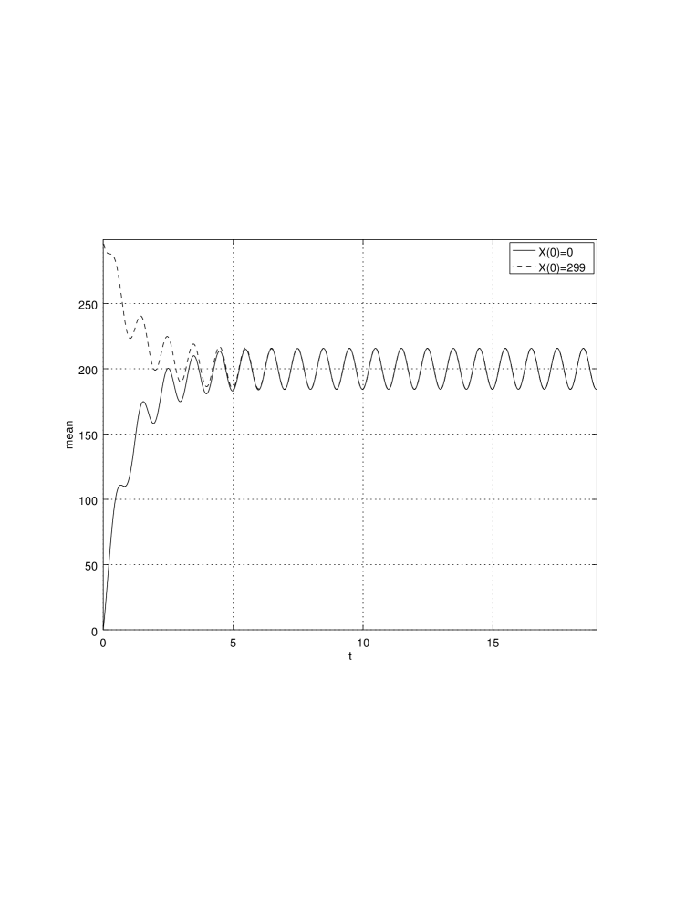
Fig. 1: Example 1. The mean $E(t,0)$ and $E(t,N)$ for the original process $t\in[0,19]$, $\omega=1$.

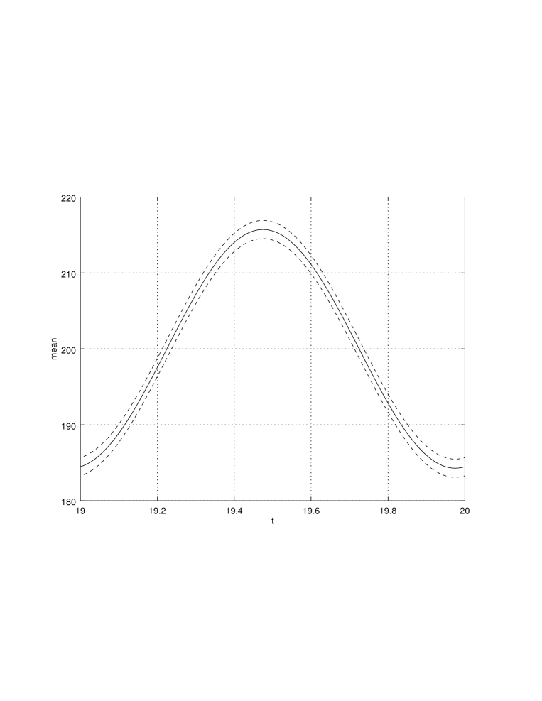
Fig. 2: Example 1. The perturbation bounds for the limit expectation $E(t,0)$, $t\in[19,20]$, $\omega=1$.

Fig. 3: Example 1. The perturbation bounds for the ’limit’ probability $\Pr(X(t)=190)$, $t\in[19,20]$, $\omega=1$.

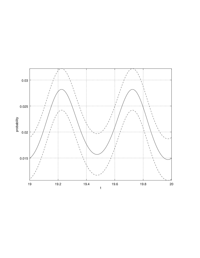
Fig. 4: Example 1. The perturbation bounds for the ’limit’ probability $\Pr(X(t)=200)$, $t\in[19,20]$, $\omega=1$.

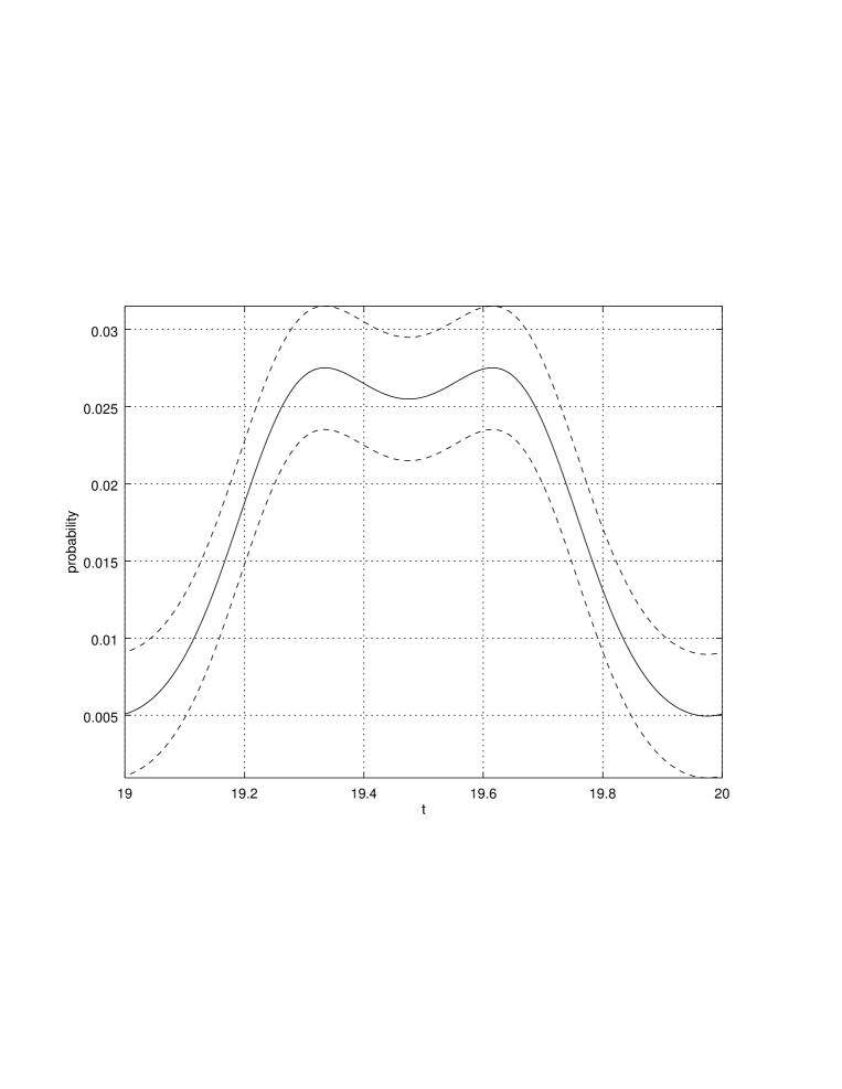
Fig. 5: Example 1. The perturbation bounds for the ’limit’ probability $\Pr(X(t)=210)$, $t\in[19,20]$, $\omega=1$.

Fig. 6: Example 1. The expectations $E(t,0)$ and $E(t,N)$ for the original process $t\in[0,18]$, $\omega=0.5$.

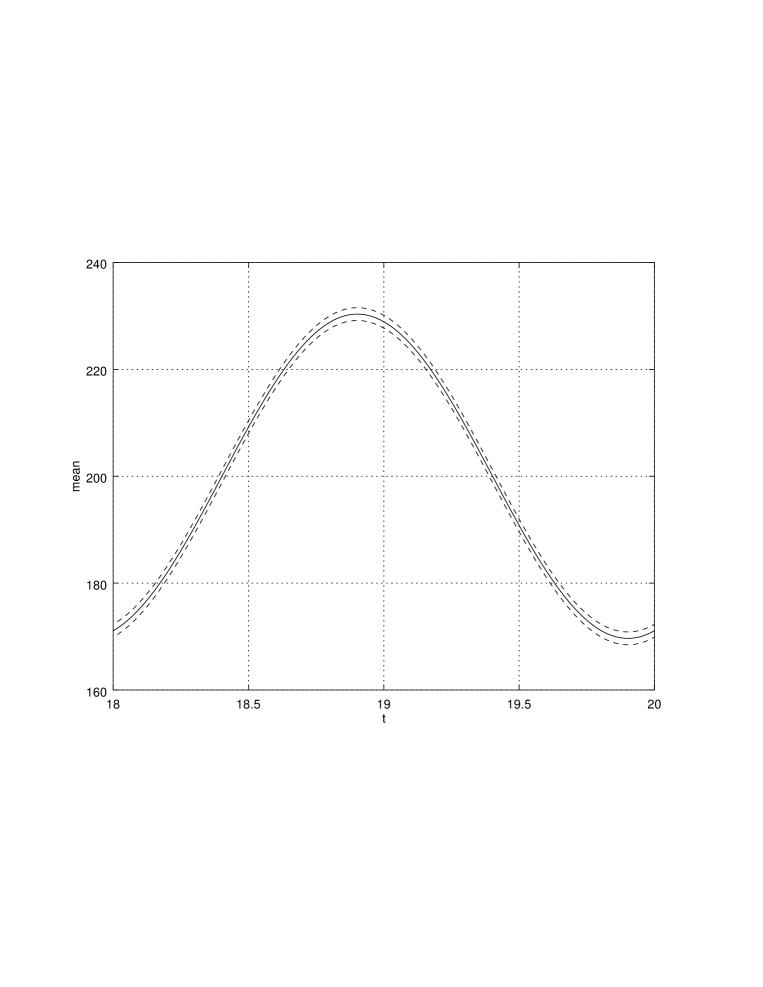
Fig. 7: Example 1. The perturbation bounds for the limit expectation $E(t,0)$, $t\in[18,20]$, $\omega=0.5$.

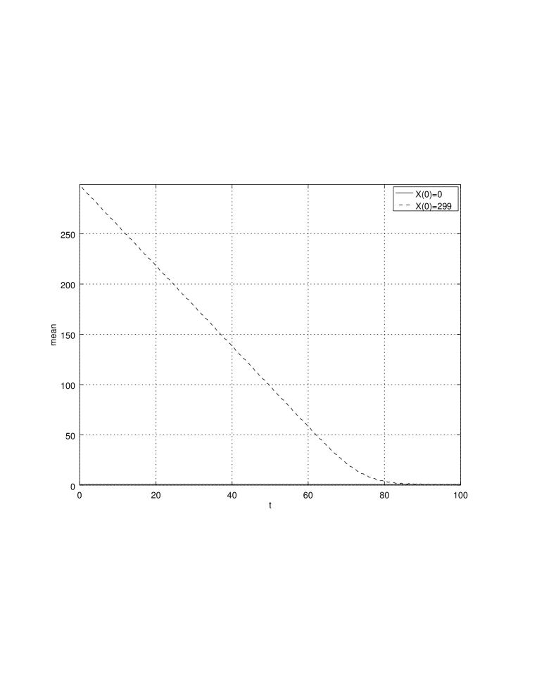
Fig. 8: Example 2. The expectations $E(t,0)$ and $E(t,299)$ for the original process $t\in[0,100]$.

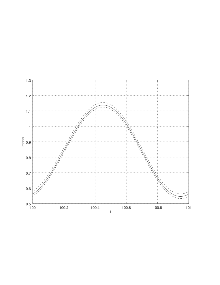
Fig. 9: Example 2. The perturbation bounds for the limit expectation $E(t,0)$, $t\in[100,101]$.

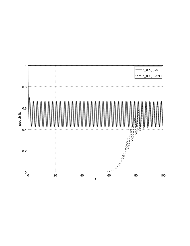
Fig. 10: Example 2. The probabilities of the empty queue for $X(0)=0$ and $X(0)=299$ for the original process $t\in[0,100]$.

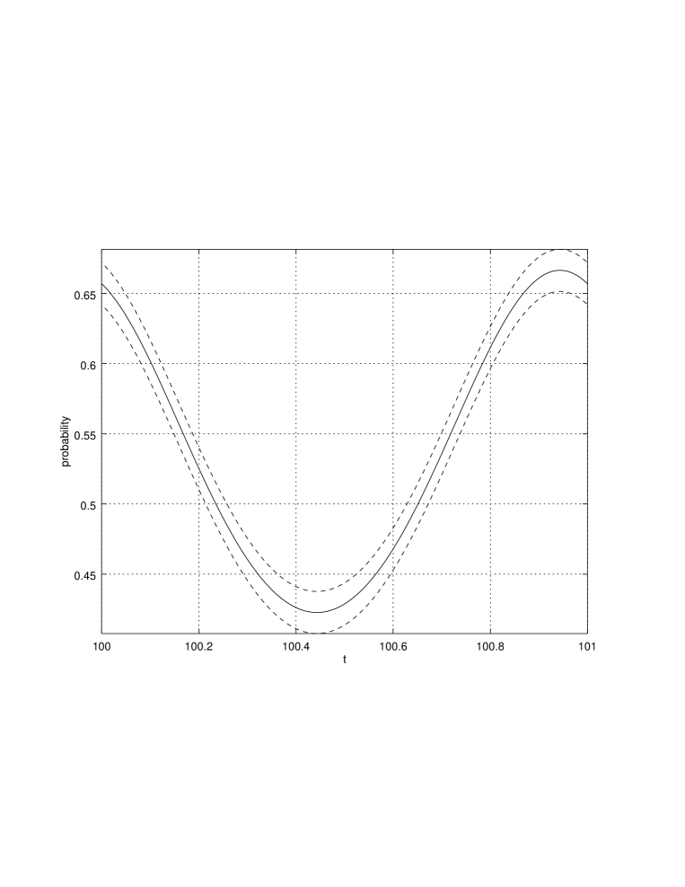
Fig. 11: Example 2. The perturbation bounds for the ’limit’ probability $\Pr(X(t)=0)$, $t\in[100,101]$.

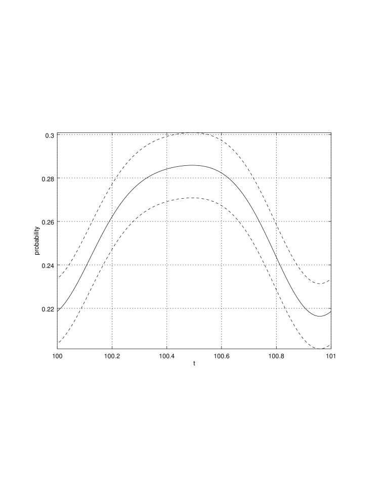
Fig. 12: Example 2. The perturbation bounds for the ’limit’ probability $\Pr(X(t)=1)$, $t\in[100,101]$.

Fig. 13: Example 2. The perturbation bounds for the ’limit’ probability $\Pr(X(t)=2)$, $t\in[100,101]$.

References

- [1] Abbas, K., Berkhout, J., Heidergott, B. (2016). A critical account of perturbation analysis of Markov chains. arXiv preprint arXiv:1609.04138.
- [2] Aldous D J., Fill J. Reversible Markov Chains and Random Walks on Graphs. Chapter 8. http://www.stat.berkeley.edu/users/aldous/RWG/book.html.
- [3] Altman E., Avrachenkov K., Núnez-Queija R. Perturbation analysis for denumerable Markov chains with application to queueing models // Adv. Appl. Probab., 2004. Vol. 36. P. 839–853.
- [4] Chen, A., Renshaw, E. The queue with mass exodus and mass arrivals when empty. Journal of Applied Probability, 34(1), 192–207 (1997)
- [5] Daleckii, J. L., Krein, M. G. Stability of solutions of differential equations in Banach space (No. 43). American Mathematical Soc. (2002)
- [6] Di Crescenzo, A., Giorno, V., Nobile, A. G., Ricciardi, L. M. A note on birth death processes with catastrophes. Statistics & Probability Letters, 78(14), 2248–2257 (2008)
- [7] Diaconis P., Stroock D. Geometric Bounds for Eigenvalues of Markov Chains // Ann. Appl. Probab., 1991. Vol. 1. P. 36–61.
- [8] Van Doorn, E. A., Zeifman, A. I., Panfilova, T. L. (2010). Bounds and asymptotics for the rate of convergence of birth-death processes. Theory of Probability & Its Applications, 54(1), 97–113.
- [9] Van Doorn, E. A. (2011). Rate of convergence to stationarity of the system M/M/N/N+R. Top, 19(2), 336–350.
- [10] Dudin, A.; Nishimura, S. A BMAP/SM/1 queueing system with Markovian arrival input of disasters. J. Appl. Probab. 1999, 36, 868–881.
- [11] Dudin, A.; Karolik,A. BMAP/SM/1 queue with Markovian input of disasters and non-instantaneous recovery. Perform. Eval. 2001, 45, 19–32.
- [12] Ferre D., Herve L., Ledoux J. Regular perturbation of V-geometrically ergodic Markov chains // J. Appl. Probab., 2013. Vol. 50. P. 184–194.
- [13] B. V. Gnedenko and I. P. Makarov, Properties of a problem with losses in the case of periodic intensities, Diff. equations. 7 (1971), pp. 1696–1698 (in Russian).
- [14] Gnedenko B., Soloviev A. On the conditions of the existence of final probabilities for a Markov process // Math. Oper. Stat., 1973. Vol. 4. P. 379–390.
- [15] Gnedenko B. V., Korolev V. Yu. Random Summation: Limit Theorems and Applications. – Boca Raton: CRC Press, 1996.
- [16] Gnedenko D. B. On a generalization of Erlang formulae // Zastosow. Mat., 1972. Vol. 12. P. 239–242.
- [17] Granovsky B. L., Zeifman A. I. Nonstationary Queues: Estimation of the Rate of Convergence // Queueing Syst., 2004. Vol. 46. P. 363–388.
- [18] Jiang, S., Liu, Y., Tang, Y. (2017). A unified perturbation analysis framework for countable Markov chains. Linear Algebra and its Applications, 529, 413-440.
- [19] V. V. Kalashnikov, Qualitative analysis of the behavior of complex systems by the method of test functions, M., Nauka, 1978 (in Russian).
- [20] Kalashnikov V. V., Zolotarev V. M. (eds.). Stability problems for stochastic models // Lecture Notes in Mathematics, 1983. Vol. 982.
- [21] N. V. Kartashov, Strongly stable Markov chains, Journal of Soviet Mathematics, 34, (1986) pp. 1493–1498 (published in Russian in 1981).
- [22] N. V. Kartashov, Criteria for uniform ergodicity and strong stability of Markov chains with a common phase space, Theory Probab. Appl., 30 (1985), pp. 71–89.
- [23] Kartashov N. V. Strong stable Markov chains. – Utrecht: VSP; Kiev: TBiMC, 1996.
- [24] Li, J., Zhang, L. Queue with catastrophes and state-dependent control at idle time. Frontiers of Mathematics in China, 12(6), 1427–1439 (2017)
- [25] Liu, Y. Perturbation bounds for the stationary distributions of Markov chains // SIAM J. Matrix Anal. & Appl., 2012. Vol. 33. P. 1057–1074.
- [26] Liu, Y., Li, W. (2018). Error bounds for augmented truncation approximations of Markov chains via the perturbation method. Advances in Applied Probability, 50(2), 645-669.
- [27] Massey W. A., Whitt W. Uniform acceleration expansions for Markov chains with time-varying rates // Ann. Appl. Probab., 1998. Vol. 8. P. 1130–1155.
- [28] Medina-Aguayo, F., Rudolf, D., Schweizer, N. (2019). Perturbation bounds for Monte Carlo within Metropolis via restricted approximations. Stochastic Processes and their Applications.
- [29] Meyn S. P., Tweedie R. L. Computable bounds for geometric convergence rates of Markov chains // Ann. Appl. Probab., 1994. Vol. 4. P. 981–1012.
- [30] Mitrophanov A. Yu. Stability and exponential convergence of continuous-time Markov chains // J. Appl. Probab., 2003. Vol. 40. P. 970–979.
- [31] Mitrophanov A. Yu. The spectral gap and perturbation bounds for reversible continuous-time Markov chains // J. Appl. Probab., 2004. Vol. 41. P. 1219–1222.
- [32] Mitrophanov A. Yu. Ergodicity coefficient and perturbation bounds for continuous-time Markov chains // Math. Inequal. Appl., 2005. Vol. 8. P. 159–168.
- [33] A. Yu. Mitrophanov, Estimates of sensitivity to perturbations for finite homogeneous continuous-time Markov chains, Theory Probab. Appl. 50 (2006), pp. 319–326.
- [34] Mitrophanov, A.Y. Connection between the Rate of Convergence to Stationarity and Stability to Perturbations for Stochastic and Deterministic Systems. In Proceedings of the 38th International Conference Dynamics Days Europe (DDE 2018), Loughborough, UK, 3–7 September 2018.
- [35] Mouhoubi Z., Aïssani D. New perturbation bounds for denumerable Markov chains // Linear Algebra and its Applications, 2010. Vol. 432. P. 1627–1649.
- [36] Negrea, J., Rosenthal, J. S. (2017). Error bounds for approximations of geometrically ergodic Markov chains. arXiv preprint arXiv:1702.07441.
- [37] Nelson, R., Towsley, D., Tantawi, A. N. (1988). Performance analysis of parallel processing systems. IEEE Transactions on software engineering, 14(4), 532-540.
- [38] Rudolf, D., Schweizer, N. (2018). Perturbation theory for Markov chains via Wasserstein distance. Bernoulli, 24(4A), 2610-2639.
- [39] Ya. A. Satin, A. I. Zeifman, A. V. Korotysheva, S. Ya. Shorgin, On a class of Markovian queues, Informatics and its applications, 5. No. 4 (2011), pp. 6–12 (in Russian).
- [40] Ya. A. Satin, A. I. Zeifman and A. V. Korotysheva, On the rate of convergence and truncations for a class of Markovian queueing systems, Th. Prob. Appl. (2013)
- [41] Satin, Y., Zeifman, A., Kryukova, A. (2019). On the Rate of Convergence and Limiting Characteristics for a Nonstationary Queueing Model. Mathematics, 7(8), 678.
- [42] Shao, J., Yuan, C. (2019). Stability of regime-switching processes under perturbation of transition rate matrices. Nonlinear Analysis: Hybrid Systems, 33, 211–226.
- [43] D. Stoyan, Qualitative Eigenschaften und Abschätzungen stochastischer Modelle, Berlin: Akademie-Verlag, 1977 (in German).
- [44] Thiede, E., Van Koten, B., Weare, J. (2015). Sharp entrywise perturbation bounds for Markov chains. SIAM Journal on Matrix Analysis and Applications, 36(3), 917-941.
- [45] Truquet, L. (2017). A perturbation analysis of some Markov chains models with time-varying parameters. arXiv preprint arXiv:1706.03214.
- [46] Vial, D., Subramanian, V. (2019). Restart perturbations for lazy, reversible Markov chains: trichotomy and pre-cutoff equivalence. arXiv preprint arXiv:1907.02926.
- [47] Zeifman A. I. Stability for contionuous-time nonhomogeneous Markov chains // Lecture Notes in Mathematics, 1985. Vol. 1233. P. 401–414.
- [48] A. I. Zeifman, Qualitative properties of inhomogeneous birth and death processes, Journal of Soviet Mathematics, 57 (1991), pp. 3217–3224 (published in Russian in 1988).
- [49] Zeifman A. I., Isaacson D. On strong ergodicity for nonhomogeneous continuous-time Markov chains // Stoch. Proc. Appl., 1994. Vol. 50. P. 263–273.
- [50] Zeifman A. I. Upper and lower bounds on the rate of convergence for nonhomogeneous birth and death processes // Stoch. Proc. Appl., 1995. Vol. 59. P. 157–173.
- [51] Zeifman A. I. Stability of birth and death processes // J. Math. Sci., 1998. Vol. 91. P. 3023–3031.
- [52] Zeifman A. I., Leorato S., Orsingher E., Satin Ya., Shilova G. Some universal limits for nonhomogeneous birth and death processes // Queueing Syst., 2006. Vol. 52. P. 139–151.
- [53] Zeifman, A. I. (2009). On the nonstationary Erlang loss model. Automation and Remote Control, 70(12), 2003–2012.
- [54] A. Zeifman, A. Korotysheva and Y. Satin, "On stability for Mt/Mt/N/N queue,"International Congress on Ultra Modern Telecommunications and Control Systems, Moscow, 2010, pp. 1102–1105. doi: 10.1109/ICUMT.2010.5676515
- [55] Zeifman, A. I., Korotysheva, A. V., Panfilova, T. Y. L., Shorgin, S. Y. (2011). Stability bounds for some queueing systems with catastrophes. Informatika i Ee Primeneniya [Informatics and its Applications], 5(3), 27-33.
- [56] A. Zeifman, S. Shorgin, A. Korotysheva, V. Bening. 2011. Stability bounds for Mt/Mt/N/N + R queue. In Proceedings of the 5th International ICST Conference on Performance Evaluation Methodologies and Tools (VALUETOOLS ’11). ICST (Institute for Computer Sciences, Social-Informatics and Telecommunications Engineering), ICST, Brussels, Belgium, Belgium, 434–438.
- [57] Zeifman A. I., Korotysheva A. Perturbation bounds for queue with catastrophes // Stochastic models, 2012. Vol. 28. P. 49–62.
- [58] Zeifman, A., Satin, Ya., Korolev, V., Shorgin, S. On truncations for weakly ergodic inhomogeneous birth and death processes. International Journal of Applied Mathematics and Computer Science, 24, 503–518 (2014)
- [59] Zeifman, A. I., Korolev, V. Y. E., Korotysheva, A. V., Shorgin, S. Y. (2014). General bounds for nonstationary continuous-time Markov chains. Informatika i Ee Primeneniya [Informatics and its Applications], 8(1), 106–117.
- [60] Zeifman, A. I., Korolev, V. Y. On perturbation bounds for continuous-time Markov chains. Stat. Probab. Lett. 88, 66–72. (2014)
- [61] Zeifman, A., Korotysheva, A. , Korolev, V., Satin, Y., Bening, V. Perturbation bounds and truncations for a class of Markovian queues. Queueing Syst. 76, 205–221. (2014)
- [62] Zeifman, A., Korotysheva, A., Satin, Y., Razumchik, R., Korolev, V., Shorgin, S. (2017). Ergodicity and truncation bounds for inhomogeneous birth and death processes with additional transitions from and to origin. Stochastic Models, 33(4), 598-616.
- [63] Zeifman, A. I., Korotysheva, A., Satin, Y., Kiseleva, K., Korolev, V., Shorgin, S. (2017, May). Bounds For Markovian Queues With Possible Catastrophes. In ECMS (pp. 628-634), http://www.scs-europe.net/dlib/2017/2017-0628.htm
- [64] Zeifman, A. I., Korotysheva, A. V., Korolev, V. Yu., Satin, Ya. A. Truncation bounds for approximations of inhomogeneous continuous-time Markov chains. Theory of Probability and Applications, 61, 513–520 (2017)
- [65] Zeifman, A., Sipin, A., Korolev, V., Shilova, G., Kiseleva, K., Korotysheva, A., Satin, Y. On Sharp Bounds on the Rate of Convergence for Finite Continuous-Time Markovian Queueing Models. In: Moreno-Diaz R., Pichler F., Quesada-Arencibia A. (eds) Computer Aided Systems Theory EUROCAST 2017. Lecture Notes in Computer Science, vol 10672. Springer, Cham, 20–28. (2018)
- [66] Zeifman, A., Razumchik, R., Satin, Y., Kiseleva, K., Korotysheva, A., Korolev, V. Bounds on the Rate of Convergence for One Class of Inhomogeneous Markovian Queueing Models with Possible Batch Arrivals and Services. Int. J. Appl. Math. Comp. Sci., 28. (2018)
- [67] Zeifman, A. I., Korolev, V. Y., Satin, Y. A., Kiseleva, K. M. (2018). Lower bounds for the rate of convergence for continuous-time inhomogeneous Markov chains with a finite state space. Statistics & Probability Letters, 137, 84–90.
- [68] Zeifman, A., Satin, Y., Kiseleva, K., Korolev, V., Panfilova, T. On limiting characteristics for a non-stationary two-processor heterogeneous system. Applied Mathematics and Computation, 351, 48–65. (2019)
- [69] Zhang, L., Li, J. The M/M/c queue with mass exodus and mass arrivals when empty. Journal of Applied Probability, 52, 990–1002 (2015)
- [70] Zheng, Z., Honnappa, H., Glynn, P. W. (2018). Approximating Performance Measures for Slowly Changing Non-stationary Markov Chains. arXiv preprint arXiv:1805.01662.
- [71] Zolotarev V. M. Quantitative estimates for the continuity property of queueing systems of type // Theory Probab. Appl., 1977. Vol. 22. P. 679–691.