Ground states of dipolar spin-orbit-coupled Bose-Einstein condensates in a toroidal trap

Abstract

We investigate the ground-state structures of dipolar spin-orbit-coupled Bose-Einstein condensates in a toroidal trap. Combined effects of dipole-dipole interaction (DDI) and spin-orbit coupling (SOC) on the ground states of the system are discussed. A ground-state phase diagram is obtained as a function of the SOC and DDI strengths. As two new degrees of freedom, the DDI and SOC can be used to obtain the desired ground-state phases and to control the phase transition between various ground states. In particular, the system displays exotic topological structures and spin textures, such as half-quantum vortex, vortex string, vortex necklace, complex vortex lattice including giant vortex and hidden antivortex chains, different skyrmions, meron (half-skyrmion)-antimeron (half-antiskyrmion) necklace, and composite meron-antimeron lattice.

1 Introduction

The past few decades have witnessed unprecedented advances in experimental and theoretical investigations on ultracold atomic gases [1, 2]. In general, the contact interatomic interactions that can be controlled by Feshbach resonance play a key role in the physical properties of Bose-Einstein condensates (BECs). For most of alkali atomic BECs, the two-body contact interaction between atoms is crucially determined by the $s$-wave scattering length and the other interactions can be neglected. However, for the BECs made of atoms with large magnetic dipole moments there are not only contact interaction but also strong dipole-dipole interaction (DDI) [3]. The magnetic DDI can be attractive or repulsive depending on the orientation of atomic dipole moments, the relative position of particles and the geometric structure of the system. Recent experimental and theoretical studies of dipolar quantum gases with chromium [4], dysprosium [5], and erbium atoms [6] show that DDI can have pronounced effects on the mean-field ground states, Bogoliubov spectra, many-body stationary states, and dynamics of the BECs or degenerate Fermi gases [7, 8, 9, 10, 11, 12, 13, 14, 15]. These remarkable effects include ferrosuperfluid [4], droplet crystals [9], dipolar superfluid [14], flat Landau levels [16], and roton mode in a dipolar quantum gas [17].

On the other hand, spin-orbit coupled quantum gases have also become one of the focuses in cold atom physics in recent years [18]. Compared with the natural solid state system with unavoidable impurities and disorder, the ultracold atomic gases with spin-orbit coupling (SOC) provide a new testing ground for studying novel SOC physics and potential applications due to their ultrahigh purity, experimental precise controllability and excellent theoretical description [19, 20, 21, 22, 23, 24], particularly for BECs [25, 26, 27, 28, 29, 30, 31, 32, 33, 34]. In a realistic physical system, ultracold atomic gases are confined in an external potential. As a matter of fact, the presence of various external potentials leads to rich physics because different trapping potentials can dramatically affect the physical properties of the BECs. For instance, the breathing mode and scissors mode in a harmonic trap [35], the quantum phase transition from a superfluid to a Mott insulator in an optical lattice [36], and the hidden vortices [37, 38, 39, 40] and macroscopic quantum self-trapping [41] in a double-well potential have been revealed in the literature. Recently, a new type of nonsimply connected trapping potential, i.e., a toroidal potential, has become experimentally available due to the development of different techniques. The toroidal potential allows nontrivial topological structures, unusual quantum dynamics and tunable features [42, 43, 44, 45, 46, 47].

In this work, we study the ground-state properties of dipolar BECs with SOC in a toroidal trap. To obtain the ground state of the system, we numerically calculate the coupled Gross-Pitaevskii (GP) equations by using standard imaginary-time propagation method [26, 48]. The results show that one can obtain the desired ground-state phases by controlling the DDI strength and SOC strength and regulating the phase transition between different ground states. In addition, we find that the system supports rich topological structures and exotic spin textures which are expected to be observed in the future cold-atom experiments. In the rest of this paper, it is organized as follows. The theoretical model is presented in Sec. 2. The results and discussion are shown in Sec. 3. Finally we give a brief summary in Sec. 4.

2 Model

We consider quasi-two-dimensional (quasi-2D) two-component dipolar BECs with Rashba SOC in a toroidal trap and with strong confinement in the $z$-direction. In the frame of mean-field theory, the dynamics of the system is described by the coupled 2D GP equations,

$$i\hbar\frac{\partial\psi_{j}}{\partial t} = [-\frac{\hbar^{2}}{2m}\nabla^{2}+V(r)+g_{j}\left|\psi_{j}\right|^{2}+g_{j(3-j)}\left|\psi_{(3-j)}\right|^{2}$$ (1)

$$+v_{so}+\phi_{j}+\phi_{j(3-j)}]\psi_{j},$$

where $\psi_{j}(r)$ $(j=1,2)$ denote the two-component wave functions, and the normalization condition is given by $\int[\left|\psi_{1}\right|^{2}+\left|\psi_{2}\right|^{2}]dr=N$ with $N$ being the number of atoms. $g_{j}$ $=\sqrt{8\pi}\hbar^{2}a_{j}/ma_{z}$ $(j=1,2)$ and $g_{12}$ $=g_{21}=\sqrt{8\pi}\hbar^{2}a_{12}/ma_{z}$ represent the quasi-2D intra- and intercomponent coupling strengths [49], where we have assumed that the two component atoms have the same mass $m$, $a_{z}=\sqrt{\hbar/m\omega_{z}}$with $\omega_{z}$ being the harmonic trap frequency in the $z$ direction, and $a_{j}$ $(j=1,2)$ and $a_{12}$ denote the $s$-wave scattering lengths between intra- and intercomponent atoms, respectively. The Rashba SOC is expressed by $v_{so}=-i\hbar k(\hat{\sigma}_{x}\partial_{y}-\hat{\sigma}_{y}\partial_{x})$ with $\hat{\sigma}_{x,y}$ being Pauli matrices and $k$ being the isotropic SOC strength. The toroidal trap is given by [46, 50]

$$V(r)=\frac{1}{2}\hbar\omega_{\bot}\left[V_{0}\left(\frac{r^{2}}{a_{0}^{2}}-r_{0}\right)^{2}\right],$$ (2)

where $\omega_{\bot}$ is the radial oscillation frequency, $r=\sqrt{x^{2}+y^{2}}$, and $a_{0}=\sqrt{\hbar/m\omega_{\bot}}$. $V_{0}$ and $r_{0}$ represent the central height and the width of the toroidal trap, respectively. $\phi_{j}(x,y)$ $(j=1,2)$ and $\phi_{12}(x,y)=\phi_{21}(x,y)$ denote the DDIs of intraspecies and interspecies, respectively, and they can be expressed as [3, 51]

$$\phi_{j} = c_{j}\int d\mathbf{r}^{\prime}U_{dd}(\mathbf{r}-\mathbf{r}^{\prime})\left|\psi_{j}(\mathbf{r}^{\prime})\right|^{2},$$ (3)

$$\phi_{j(3-j)} = c_{12}\int d\mathbf{r}^{\prime}U_{dd}(\mathbf{r}-\mathbf{r}^{\prime})\left|\psi_{(3-j)}(\mathbf{r}^{\prime})\right|^{2}.$$ (4)

Here $c_{j}=\mu_{0}\mu_{j}^{2}/4\pi$ $(j=1,2)$ and $c_{12}=\mu_{0}\mu_{1}\mu_{2}/4\pi$ are magnetic dipole constants of intraspecies and interspecies, $\mu_{0}$ is the vacuum magnetic permeability, and $\mu_{j}$ $(j=1,2)$ represent magnetic dipole moments of the two components, respectively. Let us consider the simplest case in which the dipoles are polarized. Then $U_{dd}(\mathbf{R})$ is given by [52]

$$U_{dd}(\mathbf{R})=(1-3\cos^{2}\theta)/R^{3},$$ (5)

where $\theta$ is the angle between the direction of polarization and the relative position of atoms.

For the sake of discussion, we assume DDI exists only in component 1 and the magnetic dipole moment is in the $z$ direction, i.e., $\phi_{2}=\phi_{12}=\phi_{21}=0$. In view of the numerical computations, it is convenient to introduce the following notations $\tilde{r}=r/a_{0},\tilde{t}=\omega_{\bot}t,$ $\tilde{V}(r)=V(r)/\hbar\omega_{\bot},$ $\tilde{\phi}_{1}=\phi_{1}/\hbar\omega_{\bot}$, $\tilde{\psi}_{j}=\psi_{j}a_{0}/\sqrt{N}(j=1,2)$, $\beta_{jj}=g_{j}Nm/\hbar^{2}$ $(j=1,2)$ and $\beta_{12}=g_{12}Nm/\hbar^{2}$, and then we obtain the dimensionless coupled GP equations,

$$i\partial_{t}\psi_{1} = \left(-\frac{1}{2}\nabla^{2}+V+\beta_{11}\left|\psi_{1}\right|^{2}+\beta_{12}\left|\psi_{2}\right|^{2}+\phi_{1}\right)\psi_{1}$$ (6)

$$+k\left(\partial_{x}-i\partial_{y}\right)\psi_{2},$$

$$i\partial_{t}\psi_{2} = \left(-\frac{1}{2}\nabla^{2}+V+\beta_{22}\left|\psi_{2}\right|^{2}+\beta_{12}\left|\psi_{1}\right|^{2}\right)\psi_{2}$$ (7)

$$-k(\partial_{x}+i\partial_{y})\psi_{1}.$$

For simplicity the tilde is omitted throughout this paper. Here $\beta_{jj}$ $(j=1,2)$ and $\beta_{12}$ are dimensionless intra- and interspecies coupling strengths for the contact interactions, and $k$ is the dimensionless SOC strength as mentioned before. For the present dipolar BECs, the system interactions include s-wave interactions, DDI and SOC. It is convenient to introduce a dimensionless quantity to describe the magnitude of the DDI relative to the contact interaction [52, 53, 54],

$$\varepsilon_{dd}=a_{dd}/a_{1}=\frac{\mu_{0}\mu_{1}^{2}m}{12\pi\hbar^{2}a_{1}},$$ (8)

where $a_{dd}\$denotes the scattering length characterizing the DDI. Here we assume that the dipoles are polarized along the $z$ direction, i.e., these dipoles are arranged side by side along the $z$ axis. In this context, the DDI becomes an isotropic repulsion (or attraction) and can be equivalent to a contact interaction. Therefore, the DDI can be rewritten as the form of effective contact interaction [53, 54]

$$\phi_{1}=\beta_{11}\varepsilon_{dd}\left|\psi_{1}\right|^{2},$$ (9)

where the DDI is repulsive for $\varepsilon_{dd}>0$ and attractive for $\varepsilon_{dd}<0$ when $a_{1}>0$. Obviously the total interaction coefficient between atoms for component $1$ can be expressed by $(1+\varepsilon_{dd})\beta_{11}$. Thus one can obtain and control different ground-state phases by varying the DDI strength $\varepsilon_{dd}$, the SOC strength $k$, and the interaction strengths $\beta_{11}$, $\beta_{22}$ and $\beta_{12}$.

In order to further understand the topological properties of the system, we adopt a nonlinear Sigma model [55, 46] in which a normalized complex-valued spinor $\mathbf{\chi}=[\chi_{1},\chi_{2}]^{T}$ with $|\chi_{1}|^{2}+|\chi_{2}|^{2}=1$ is introduced. The total density of the system is expressed by $\rho=|\psi_{1}|^{2}+|\psi_{2}|^{2}$, where the corresponding two-component wave functions are $\psi_{1}=\sqrt{\rho}\chi_{1}$ and $\psi_{2}=\sqrt{\rho}\chi_{2}$, respectively. The spin density is given by $\mathbf{S}=\overline{\mathbf{\chi}}\mathbf{\sigma\chi}$ with $\mathbf{\sigma}=(\sigma_{x},\sigma_{y},\sigma_{z})$ being the Pauli matrices. The components of $\mathbf{S}$ are defined as

$$S_{x} = \chi_{1}^{\ast}\chi_{2}+\chi_{2}^{\ast}\chi_{1},$$ (10)

$$S_{y} = i(\chi_{2}^{\ast}\chi_{1}-\chi_{1}^{\ast}\chi_{2}),$$ (11)

$$S_{z} = |\chi_{1}|^{2}-|\chi_{2}|^{2},$$ (12)

with $|\mathbf{S}|=\sqrt{S_{x}^{2}+S_{y}^{2}+S_{z}^{2}}=1$. The spacial distribution of the topological structure of the system can be characterized by the topological charge density

$$q(r)=\frac{1}{4\pi}\mathbf{S\bullet}\left(\frac{\partial\mathbf{S}}{\partial x}\times\frac{\partial\mathbf{S}}{\partial y}\right),$$ (13)

and the topological charge is given by $Q=\int q(r)dxdy.$

3 Results and discussion

In the absence of DDI and SOC, the two-component BECs in a toroidal trap support two typical ground-state phases: phase mixing (component mixing) and phase separation (component demixing) [45, 46]. The two different types of ground states can be achieved by controlling the intra- and interspecies contact interactions. Here we focus on the case of strong confinement of the toroidal trap, where $V_{0}=5$ and $r_{0}=3$. Using the standard imaginary time evolution [26, 48] based on the Peaceman–Rachford algorithm [56, 57], we can obtain the ground-state structures of two-component BECs with DDI and SOC in a toroidal trap by numerical computation. The main idea of the Peaceman–Rachford algorithm is to convert a 2D problem into two 1D problems, and the algorithm can be easily extended to 3D cases. The imaginary-time propagation method with the Peaceman–Rachford algorithm has good convergence, high accuracy and strong stability. A test for the method is given by the fast convergent values of the total energy and component wave functions of the system. A second test of convergence and accuracy is provided by the virial theorem, which fixes rigorous relationships among the different contributions to the kinetic and potential energies of the system. In addition, it can also be tested by the same convergent results for different trial wave functions. All the tests have been confirmed in our numerical simulation. In order to highlight the new effects resulted from the DDI and SOC, without loss of generality we fix the interaction parameters $\beta_{11}=100$, $\beta_{22}=150$ and $\beta_{12}=200$ throughout this paper, and vary the DDI strength $\varepsilon_{dd}$ or the SOC strength $k$. In fact, our simulation shows that there exist similar phase structures for the other combination cases of contact interaction parameters.

3.1 Ground-state structures

Inspired by Ref. [10], we give the ground-state phase diagram spanned by the SOC strength $k$ and the DDI strength $\varepsilon_{dd}$ in Fig. 1. There are eight different phases marked by A-H, which differ in terms of their density profiles and phase distributions. In the following discussion, we will give a detailed description of each phase. The density and the phase profiles of the eight different phases A-H in Fig. 1 are shown in Figs. 2(a)-2(e) and Figs. 3(b), 3(c) and 3(f), respectively.

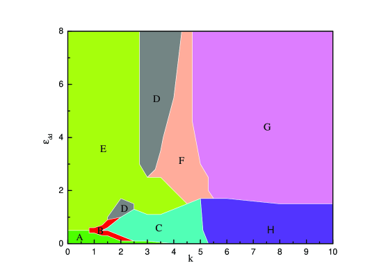
Figure 1: (Color online) Ground-state phase diagram of the spin-orbit coupled dipolar BEC with respect to $k$ and $\varepsilon_{dd}$ for $\beta_{11}=100$, $\beta_{22}=150$ and $\beta_{12}=200$. There are eight different phases marked by A-H.

We start from the case where the SOC and the DDI are weak, which is denoted by the region A in Fig. 1. In this phase, the density distributions of the two components display layer-segregated symmetry preserving annular structures [see the top two rows in Fig. 2(a)], which is mainly due to the strong repulsive interspecies contact interaction $\beta_{12}^{2}>\beta_{11}\beta_{22}$ and the tight binding of the toroidal trap. From the corresponding phase distributions in rows 3 and 4 of Fig. 2, we observe that the value of the phase changes continuously from $-\pi$ (blue) to $\pi$ (red), and the end point of the boundary between a $\pi$ phase line and a $-\pi$ phase line corresponds to a phase defect (i.e., a vortex with anticlockwise rotation or an antivortex with clockwise rotation). The topological structure of the system in Fig. 2(a) is a half-quantum vortex where there is no phase defect in the dipolar component (component 1) while there is an obvious vortex in the non-dipolar component (component 2). Here the half-quantum vortex is different from the conventional Anderson–Toulouse coreless vortex [58, 59] due to the presence of the toroidal trap. For the latter case, the vortex core of one component is usually filled with the other nonrotating component. With the slightly strong inclusion of SOC and DDI, the A phase transforms to the B phase, as shown in Fig. 1. The component densities evolve into separated stripe-like patterns or block-like patterns, and some phase defects are generated in the system [see Fig. 2(b)]. With an increase in the strength of the SOC, the C phase emerges as the ground state, as shown in Fig. 1. Typical density distributions are shown in Fig. 2 (c), in which the interlaced and separated petal structures in the component density distributions become quite pronounced, in the mean time, there is a triply quantized giant vortex in the central region of the phase distribution of the dipolar component, followed successively by a hidden antivortex necklace [37, 40] in the external region and ghost vortex necklace as well as ghost antivortex necklace [49] in the further boundary regions. By comparison, the central region of the phase profile of component 2 is occupied by a triply quantized giant antivortex with a hidden vortex necklace distributing in the outer region and ghost antivortex as well as ghost vortex necklaces in the further boundary regions. These phase defects constitute nucleated vortices and antivortices on the whole. This feature is evidently different from the case of two-component spin-orbit coupled BECs in a harmonic trap [29]. For the latter case, only conventional stripe phase and segregated symmetry preserving phase with giant skyrmion can be created when $\beta_{12}^{2}>\beta_{11}\beta_{22}$. Physically, here the special petal phase is a result of the combined effect of DDI, SOC, toroidal trap and strong interspecies repulsion.

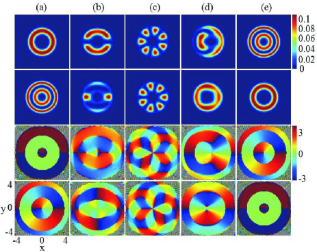
Figure 2: (Color online) Ground states of two-component BECs with DDI and SOC in a toroidal trap, where $\beta_{11}=100$, $\beta_{22}=150$, $\beta_{12}=200$, and $k=2$. (a) $\varepsilon_{dd}=0$, (b) $\varepsilon_{dd}=0.2$, (c) $\varepsilon_{dd}=0.5$. (d) $\varepsilon_{dd}=1.5$ and (e) $\varepsilon_{dd}=2$. The rows from top to bottom denote $\left|\psi_{1}\right|^{2}$, $\left|\psi_{2}\right|^{2}$, arg$\psi_{1}$, and arg$\psi_{2}$, respectively. The unit length is $a_{0}$. The value of the phase in the phase distributions (bottom two rows) changes continuously from $-\pi$ (blue) to $\pi$ (red), and the end point of the boundary between a $\pi$ phase line and a $-\pi$ phase line corresponds to a phase defect (i.e., a vortex with anticlockwise rotation or an antivortex with clockwise rotation).

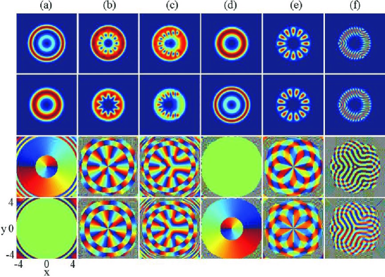
Figure 3: (Color online) Ground states of two-component BECs with various DDI and SOC strengths in a toroidal trap, where the contact interaction parameters are the same as those in Fig. 1. (a) $\varepsilon_{dd}=6$, $k=0.5$, (b) $\varepsilon_{dd}=6$, $k=4.5$, (c) $\varepsilon_{dd}=6$, $k=5$, (d) $\varepsilon_{dd}=0.3$, $k=0.5$, (e) $\varepsilon_{dd}=0.3$, $k=4$, and (f) $\varepsilon_{dd}=0.3$, $k=10$. The rows from top to bottom denote $\left|\psi_{1}\right|^{2}$, $\left|\psi_{2}\right|^{2}$, arg$\psi_{1}$, and arg$\psi_{2}$, respectively. The unit length is $a_{0}$. The value of the phase in the phase distributions (bottom two rows) changes continuously from $-\pi$ (blue) to $\pi$ (red), and the end point of the boundary between a $\pi$ phase line and a $-\pi$ phase line corresponds to a phase defect (i.e., a vortex with anticlockwise rotation or an antivortex with clockwise rotation).

In the limit of weak SOC and relatively strong DDI, the C phase transforms to the D phase, as shown in Fig. 1. The density and phase distributions are shown in Fig. 2 (d) where the petals in the two component densities become integrated and most of the phase defects disappear. In particular, two vortex dipoles (vortex-antivortex pairs) instead of a giant vortex (or antivortex) are formed in the density hole of component 2, which is indicated in the phase distribution of component 2. Although the density distributions in the B phase and the C phase do not have rotational symmetry, they still maintain good axial symmetry concerning the $y=0$ axis (or both the $y=0$ axis and the $x=0$ axis). In the presence of large repulsive DDI the ground states of component 1 and component 2 in this system are exchanged approximately with those in phase A, which is indicated by the E phase in Fig.1. Typical density and phase distributions of such a phase are shown in Fig. 2 (e). In addition, we find that different combinations of parameters $\beta_{11}$ and $\varepsilon_{dd}$ with the fixed other parameters may lead to the same ground-state structures in view of the analytical effective interaction $(1+\varepsilon_{dd})\beta_{11}$ in the dipolar component. For instance, the ground state of the system in the case of $\beta_{11}=120$ and $\varepsilon_{dd}=0.25$ is the same with that in the case of $\beta_{11}=100$ and $\varepsilon_{dd}=0.5$, where the ground-state structure for the former case is not shown here for the sake of conciseness and avoiding repetition. Furthermore, our simulation shows that the ground-state structure of the system in the presence of attractive DDI above the critical value for collapse is similar to that in Fig. 2(a).

To get a deeper physical insight into this system, we study the ground-state phase diagram with strong repulsive DDI ($\varepsilon_{dd}\geq 2.5$). With the increase of the SOC, the phase transforms from the E phase to the D phase, as shown in Fig. 1. For the relatively strong SOC ($k\geq 2.7$), the F phase emerges as the ground state of the system, as shown by the pink region in Fig. 1. Typical density and phase distributions of such a phase are shown in Fig. 3(b), where there is a giant vortex (a multiquantized vortex) [60] in the trap center surrounded by an antivortex necklace in the outer region in each component. As the SOC is further increased, the F phase transforms to the G phase (see the light purple region of Fig. 1). In the G phase, interlaced and crescent-shaped visible antivortex strings are formed in both the component densities, where there is a large density hole in the central region of each component [see Fig. 3(c)]. The large density hole is not a usual giant vortex or antivortex but a hidden vortex pair consisting of two singly quantized hidden vortices [37, 38, 39, 40] as shown in the phase distributions of Fig. 3(c). This phase exists for strong SOC and strong DDI, and occupies the largest region of the ground-state phase diagram in Fig. 1. Essentially, the irregular structures of the vortices and antivortices in Fig. 3(c) are caused by the complicated interplay among the DDI, SOC, contact interactions and the toroidal confinement.

Finally, we move to another limit of weak DDI. When the SOC increases, the phase transforms from A phase to B phase and then to C phase, and finally to H phase as shown in Fig. 1. In the case of $\varepsilon_{dd}=0.3$ and $k=4$, each component density develops into a necklace-like structure which is composed of 12 petals along the azimuthal direction [see Fig. 3(e)]. The similar necklace structure has also been found in the recent literature [45], where only odd petals are observed. By comparison, not only the necklace structure with odd number of petals but also that with even number of petals can be observed easily in the present system due to the presence of DDI [see Fig. 2(c) and Fig. 3(e)]. In addition, from the phase distribution of component 2, one can see that there is no any phase defect in the density hole. However, there exists a hidden vortex-antivortex necklace in the ring area where the petals are located, followed by several complicated ghost vortex necklaces or ghost vortex-antivortex necklaces in the outer region of the atom cloud. In particular, a giant vortex (a five quantized vortex) is distributed in the central region of component 1, and a hidden vortex necklace as well as a hidden vortex-antivortex necklace consisting of vortex-antivortex pairs are formed in the annular petal region. At the same time, the external region of the cloud is occupied by several composite ghost vortex-antivortex necklaces. [45]. Under the limit of strong SOC, the H phase emerges as the ground state, as shown in the Fig. 1. The density and phase distributions of H phase are shown in Fig. 3(f), where some petals are connected into curved stripes and the density distributions are evolved into several domains. Almost all the phase defects via the form of vortex-antivortex pairs are distributed randomly in the outer boundary region of the cloud except for a singly quantized vortex in the trap center for component 2.

The z component of the orbital angular momentum, $\left\langle L_{z}\right\rangle=\int\mathbf{\Psi}^{\dagger}(\mathbf{r})(xp_{y}-yp_{x})\mathbf{\Psi}(\mathbf{r})d\mathbf{r}$ with $\mathbf{\Psi}(\mathbf{r})=(\psi_{1}$,$\psi_{2})^{\text{T}}$, is important in considering this system. Figure 4 displays $\left\langle L_{z}\right\rangle$ as a function of $k$ for $\varepsilon_{dd}=1$ being fixed. The E phase has less angular momentum due to there being only one vortex in component 2. The first rapid increase in $\left\langle L_{z}\right\rangle$ occurs in the D phase $(1.5\leq k\leq 2)$. The angular momentum of the C phase has increasing trend, because the two components have increasing multiplequantum vortices which carry angular momentum. In the H phase, $\left\langle L_{z}\right\rangle$ decrease at $k$ $\simeq 5.5$ as the central region of component 2 has no any phase defect. The maximum of $\left\langle L_{z}\right\rangle$ is attained at $k$ $\simeq 6.5$, because the two component have many vortices which carry a lot of angular momentum. When $k$ $\simeq 7.5$, $\left\langle L_{z}\right\rangle$ decreases and the reason is similar to the case of $k$ $\simeq 5.5$.

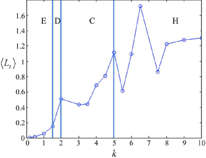
Figure 4: (Color online) Orbital angular momentum $\left\langle L_{z}\right\rangle$ as a function of k for $\varepsilon_{dd}=1$. The vertical lines separate the phases and the solid curve indicates the trend.

From the above analysis and discussion, the ground-state structure of the system can be transformed by adjusting the DDI strength $\varepsilon_{dd}$ or the SOC strength $k$ when the other parameters are fixed, which indicates that the DDI and SOC can be used as two new degrees of freedom to achieve the desired ground-state phases and to control the phase transition between different ground states. In addition, the exotic topological structures [especially shown in Figs. 2(b)-2(d) and Figs. 3(b), 3(c), 3(e) and 3(f)] are quite different from the ground-state structures observed in conventional SOC BECs [18, 19, 25, 26, 27, 28, 45], dipolar BECs [8, 14], and rotating two-component BECs with or without SOC (DDI) [29, 35, 37, 49, 60].

3.2 Spin textures

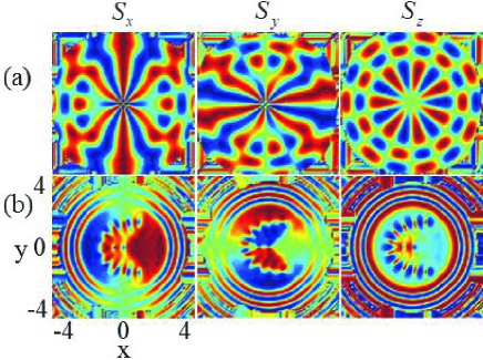
Figure 5: (Color online) Spin densities of dipolar spin-orbit coupled BECs in a toroidal trap. (a) $\varepsilon_{dd}=0.5$, $k=2$, and (b) $\varepsilon_{dd}=6$, $k=5$. The columns (from left to right) denote $S_{x},S_{y}$ and $S_{z}$ components of the spin density vector, respectively. The corresponding ground states in (a) and (b) are shown in Fig. 2(c) and Fig. 3(c), respectively. The unit length is $a_{0}$.

The typical spin density distributions are shown in Fig. 5, where $\beta_{11}=100$, $\beta_{22}=150$ and $\beta_{12}=200$. The DDI and SOC strengths in Figs. 5(a) and 5(b) are $\varepsilon_{dd}=0.5$, $k=2$, and $\varepsilon_{dd}=6$, $k=5$, respectively. The corresponding density and phase distributions are given in Fig. 2(c) and Fig. 3(c), respectively. In the spin representation, the blue region in the spin component $S_{z}$ represents spin-down ($S_{z}=-1$) and the red region denotes spin-up ($S_{z}=1$). For the case of weak DDI [see Fig. 5(a)], spin component $S_{x}$ shows an even parity distribution along both the $x$ direction and the $y$ direction while the situation is the reverse for $S_{y}$, i.e., $S_{y}$ displays an odd parity distribution along both the two directions. However, $S_{z}$ obeys an even parity distribution along the $x$ direction and an odd parity distribution along the $y$ direction. By comparison, for the case of strong DDI [see Fig. 5(b)], $S_{x}$ and $S_{z}$ display the even parity distribution along the $x$ direction while $S_{y}$ shows the odd parity distribution along the $x$ direction, where the even or odd parity distributions along the $y$ direction are lost because of the long-range and anisotropic feature of the DDI. Furthermore, one can notice that there is an obvious petal-like pattern along the radial direction in the central region and two distinct necklace-like patterns with increasing radius in the outer region in the spin component $S_{z}$ of Fig. 5(a). The alternating appearance of the blue and red petals along the radial direction as well as that of the blocks along both the azimuthal direction and the radial direction means that some regular spin domains are formed in the spin representation. The boundary region between a blue petal (or block) and a red petal (or block) actually constitutes a spin domain wall with $\left|S_{z}\right|\neq 1$. It is well known that for a system of nonrotating two-component BECs the domain wall is a typically classical Néel Wall in which the spin flips only along the vertical direction of the wall. However, our numerical simulation shows that the spin in the region of domain wall flips not only along the vertical direction (azimuthal direction) of the domain wall but also along the domain-wall direction (radial direction), which indicates that here the observed domain wall is a new type of domain wall and allows to be realized under current experimental technical conditions.

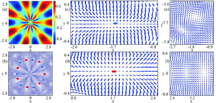
Figure 6: (Color online) Topological charge density and spin texture, where $\varepsilon_{dd}=0.5$ and $k=2$. (a) topological charge density, (b) the corresponding spin texture, and (c)-(f) the local amplifications of the spin texture. Here the blue spots denote the half-antiskyrmions (antimerons), and red spots represent the half-skyrmions (merons). The unit length is $a_{0}$.

Displayed in Figs. 6(a) and 6(b) are the topological charge density and the spin texture of the system, where $\varepsilon_{dd}=0.5$, $k=2$, and the contact interaction parameters are the same as those in Figs. 1-5. Figs. 6(c)-6(f) are the typical local enlargements of the spin texture in Fig. 6(b). The corresponding ground state and three spin components are given in Fig. 2(c) and Fig. 5(a), respectively. In Figs. 6(b)-6(d), the blue spots denote radial-in half-antiskyrmions (antimerons) [55, 61] with local topological charge $Q=-0.5$, and the red spots represent radial-out half-skyrmions (merons) [62, 63] with local topological charge $Q=0.5$. These meron-antimeron pairs (half-skyrmion and half-antiskyrmion pairs) constitute an alternating complex and fascinating meron (half-skyrmion)-antimeron (half-antiskyrmion) necklace, which, to the best of our knowledge, has not yet been reported elsewhere. In addition, there are some skyrmions (or antiskyrmions) [61, 62] with local topological charge $\left|Q\right|=1$ distributed outside of the meron (half-skyrmion)-antimeron (half-antiskyrmion) necklace, and typical local amplifications are given in Figs. 6(e) and 6(f). As a matter of fact, Fig. 6(e) describes a hyperbolic-radial(in) antiskyrmion with topological charge $Q=-1$ while Fig. 6(f) denotes a hyperbolic-radial(out) skyrmion with $Q=1$, where the former case can be regarded as a combination of two antimerons (half-antiskyrmions) and the latter case can be considered as a combination of two merons (half-skyrmions). Physically, the skyrmions or merons (half-skyrmions) in the spin textures of the present system are associated with the vortex structures in the component density profiles, and the particle density should obey the continuity condition due to the quantum fluid nature of the BECs.

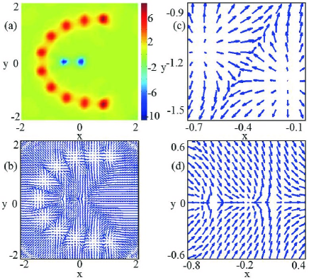
Figure 7: (Color online) Topological charge density and spin texture, where $\beta_{11}=100$, $\beta_{22}=150$, $\beta_{12}=200$, $\varepsilon_{dd}=6$, and $k=5$. (a) topological charge density, (b) the corresponding spin texture, and (c)-(d) the local amplifications of the spin texture. The unit length is $a_{0}$.

Figure 7(a) shows the topological charge density in the case of $\beta_{11}=100$, $\beta_{22}=150$, $\beta_{12}=200$, $\varepsilon_{dd}=6$, and $k=5$, where the ground state and three spin components are displayed in Fig. 3(c) and Fig. 5(b), respectively. The corresponding spin texture is shown in Fig. 7(b), and the typical local amplifications are given in Figs. 7(c) and 7(d). Our numerical calculation demonstrates that the two local enlargements in Fig. 7(c) are two merons (half-skyrmions) with each local topological charge being $Q=0.5$, which indicates that the arc configuration of the spin texture in Fig. 7(b) is a curved meron (half-skyrmion) chain. In the mean time, the computation result shows that the two local topological charges in Fig. 7(d) are both $Q=-0.5$, which means that the two spin defects in Fig. 7(b) [see also Fig. 7(a)] along the $y=0$ axis in the area surrounded by the arc configuration constitute an obvious antimeron pair (a half-antiskyrmion pair) made of two antimerons (half-antiskyrmions). Thus the curved meron chain and the antimeron pair jointly form a particular composite meron-antimeron lattice, which has not been observed in previous literature. The interesting and exotic spin textures as mentioned in Figs. 6 and 7 allow to be tested and observed in the future cold atom experiments.

4 Conclusion

We have studied the ground-state structures and spin textures of dipolar BECs with DDI and Rashba SOC in a toroidal trap. We focus on the combined effects of DDI and SOC on the ground-state properties of the system. A ground-state phase diagram was obtained with respect to the SOC and DDI strengths. It is shown that the DDI and the SOC, as two important parameters, play a key role in determining the ground-state structure of the system. Therefore they can be used to achieve the desired ground-state phases and to control the phase transition between different ground states. In addition, the system exhibits rich topological structures including Anderson-Toulouse nucleated vortex state, curved vortex string composed of vortices and antivortices, and necklace-like state with a giant vortex (or antivortex) plus hidden antivortex (or vortex) necklace as well as further ghost vortex (or antivortex) necklaces. Furthermore, the system sustains exotic spin textures, such as different skyrmions, meron (half-skyrmion)-antimeron (half-antiskyrmion) necklace, and complex meron (half–skyrmion)-antimeron (half-antiskyrmion) lattice composed of a curved meron (half-skyrmion) chain and an antimeron (half-antiskyrmion) pair. As the ground states are stable against perturbation and have longer lifetime in contrast to the other stationary states of the system, we expect that the topological structures and spin textures of the system can be observed and tested in the future experiments. These findings have greatly enriched our new understanding of topological defects and spin defects in ultracold atomic gases.

L.W. thanks W.Vincent Liu, Hui Zhai,Yongping Zhang and Malcolm Jardine for useful discussions. This work was supported by the National Natural Science Foundation of China (Grant Nos. 11475144 and 11047033), the Natural Science Foundation of Hebei Province of China (Grant Nos. A2019203049 and A2015203037), and Research Foundation of Yanshan University (Grant No. B846).

References

- [1] C. Chin, R. Grimm, P. Julienne, and E. Tiesinga, Rev. Mod. Phys. 82, 1225 (2010).
- [2] D. M. Stamper-Kurn and M. Ueda, Rev. Mod. Phys. 85, 1191 (2013).
- [3] T. Lahaye, C. Menotti, L. Santos, M. Lewenstein, and T. Pfau, Rep. Prog. Phys. 72, 126401 (2009).
- [4] T. Lahaye, T. Koch, B. Fröhlich, M. Fattori, J. Metz, A. Griesmaier, S. Giovanazzi, and T. Pfau, Nature 448, 672 (2007).
- [5] M. Lu, N. Q. Burdick, S. H. Youn, and B. L. Lev, Phys. Rev. Lett. 107, 190401 (2011).
- [6] K. Aikawa, A. Frisch, M. Mark, S. Baier, R. Grimm, and F. Ferlaino, Phys. Rev. Lett. 112, 010404 (2014).
- [7] L. Santos, G. V. Shlyapnikov, and M. Lewenstein, Phys. Rev. Lett. 90, 250403 (2003).
- [8] S. Yi and H. Pu, Phys. Rev. A 73, 061602 (2006).
- [9] H. Kadau, M. Schmitt, M. Wenzel, C. Wink, T. Maier, I. Ferrier-Barbut, and T. Pfau, Nature 530, 194 (2016).
- [10] M. Kato, X.-F. Zhang, D. Sasaki, and H. Saito, Phys. Rev. A 94, 043633 (2016).
- [11] S.-Y. Chä, and U. R. Fischer, Phys. Rev. Lett. 118, 130404 (2017).
- [12] M. O. Borgh, J. Lovegrove, and J. Ruostekoski, Phys. Rev. A 95, 053601 (2017).
- [13] H. Zou, E. Zhao, and W. V. Liu, Phys. Rev. Lett. 119, 050401 (2017).
- [14] M. Wenzel, F. Böttcher, J.-N. Schmidt, M. Eisenmann, T. Langen, T. Pfau, and I. Ferrier-Barbut, Phys. Rev. Lett. 121, 030401 (2017).
- [15] L. Jia, A.-B. Wang, and S. Yi, Phys. Rev. A 97, 043614 (2018).
- [16] X.-F. Zhou, C.Wu, G.-C. Guo, R. Wang, H. Pu, and Z.-W. Zhou, Phys. Rev. Lett. 120, 130402 (2018).
- [17] L. Chomaz, R. M. W. van Bijnen, D. Petter, G. Faraoni, S. Baier, J. H. Becher, M. J. Mark, F. Wächtler, L. Santos, and F. Ferlaino, Nat. Phys. 14, 42 (2018).
- [18] H. Zhai, Rep. Prog. Phys. 78, 026001 (2015).
- [19] Y.-J. Lin, K. Jiménez-García, and I. B. Spielman, Nature 471, 83 (2011).
- [20] C. Qu, C. Hamner, M. Gong, C. Zhang, and P. Engels, Phys. Rev. A 88, 021604(R) (2013).
- [21] Z. Wu, L. Zhang, W. Sun, X. T. Xu, B. Z. Wang, S. C. Ji, Y. Deng, S. Chen, X. J. Liu, and J. W. Pan, Science 354, 83 (2016).
- [22] L. Huang, Z. Meng, P. Wang, P. Peng, S. L. Zhang, L. Chen. D. Li, Q. Zhou, and J. Zhang, Nat. Phys. 12, 540 (2016).
- [23] S. Kolkowitz, S. L. Bromley, T. Bothwell, M. L. Wall, G. E. Marti, A. P. Koller , X. Zhang, A. M. Rey, and J. Ye, Nature 542, 66 (2017).
- [24] J. R. Li, J. Lee, W. Huang, S. Burchesky, B. Shteynas, F. C. Top, A. O.Jamison, and W. Ketterle, Nature 543, 91 (2017).
- [25] H. Hu, B. Ramachandhran, H. Pu, and X. J. Liu, Phys. Rev. Lett. 108, 010402 (2012).
- [26] Y. Zhang, L. Mao, and C. Zhang, Phys. Rev. Lett. 108, 035302 (2012).
- [27] Q. Zhu, C. Zhang, and B. Wu, Europhys. Lett. 100, 50003 (2012).
- [28] E. Ruokokoski, J. A. M. Huhtamäki, and M. Möttönen, Phys. Rev. A 86, 051607(R) (2012).
- [29] A. Aftalion and P. Mason, Phys. Rev. A 88, 023610 (2013).
- [30] Y. Xu, L. Mao, B. Wu, and C. Zhang, Phys. Rev. Lett. 113, 130404 (2014).
- [31] X. Jiang, Z. Fan, Z. Chen, W. Pang, Y. Li, and B. A. Malomed, Phys. Rev. A 93, 023633 (2016).
- [32] T. F. J. Poon and X.-J. Liu, Phys. Rev. A 93, 063420 (2016).
- [33] H. Sakaguchi and K. Umeda, J. Phys. Soc. Jpn. 85, 064402 (2016).
- [34] S. Gautam and S. K. Adhikari, Phys. Rev. A 97, 013629 (2018).
- [35] C. J. Pethick and H. Smith, Bose–Einstein Condensation in Dilute Gases (2nd ed.) (Cambridge Univ. Press, Cambridge, 2008).
- [36] M. Greiner, O. Mandel, T. Esslinger, T. W. Hänsch, and I. Bloch, Nature 415, 39 (2002).
- [37] L. Wen, H. Xiong, and B. Wu, Phys. Rev. A 82, 053627 (2010).
- [38] T. Mithun, K. Porsezian, and B. Dey, Phys. Rev. A 89, 053625 (2014).
- [39] R. M. Price, D. Trypogeorgos, D. L. Campbell, A. Putra, A. Valdés-Curiel, and I. B. Spielman, New J. Phys. 18, 113009 (2016).
- [40] L. H. Wen and X. B. Luo, Laser Phys. Lett. 9, 618 (2012).
- [41] A. Smerzi, S. Fantoni, S. Giovanazzi, and S. R. Shenoy, Phys. Rev. Lett. 79, 4950 (1997).
- [42] S. Eckel, J. G. Lee, F. Jendrzejewski, N. Murray, C. W. Clark, C. J. Lobb, W. D. Phillips, M. Edwards, and G. K. Campbell, Nature 506, 200 (2014).
- [43] A. A. Wood, B. H. J. McKellar, and A. M. Martin, Phys. Rev. Lett. 116, 250403 (2016).
- [44] X.-F. Zhang, M. Kato, W. Han, S.-G. Zhang, and H. Saito, Phys. Rev. A 95, 033620 (2017).
- [45] A. C. White, Y. P. Zhang, and T. Busch, Phys. Rev. A 95, 041604(R) (2017).
- [46] H. Wang, L. Wen, H. Yang, C. Shi, and J. Li, J. Phys. B 50, 155301 (2017).
- [47] J. L. Helm, T. P. Billam, A. Rakonjac, S. L. Cornish, and S. A. Gardiner, Phys. Rev. Lett. 120, 063201 (2018).
- [48] L. Wen and J. Li, Phys. Rev. A 90, 053621 (2014).
- [49] K. Kasamatsu, M. Tsubota, and M. Ueda, Phys. Rev. A 67, 033610 (2003).
- [50] M. Cozzini, B. Jackson, and S. Stringari, Phys. Rev. A 73, 013603 (2006).
- [51] S. Yi and L. You, Phys. Rev. A 61, 041604(R) (2000).
- [52] M. Ueda, Fundamentals and New Frontiers of Bose-Einstein Condensation (World Scientific, Singapore, 2010), Chap. 10.
- [53] Y. Kawaguchia and M. Ueda, Phys. Rep. 520, 253(2012), P309.
- [54] X.-F. Zhang, P. Zhang, G.-P. Chen, B. Dong, R.-B. Tan, and S.-G. Zhang, Acta. Phys. Sin. 6, 060302 (2015).
- [55] K. Kasamatsu, M. Tsubota, and M. Ueda, Phys. Rev. Lett. 93, 250406 (2004).
- [56] L. Wen, Y. Qiao, Y. Xu, and L. Mao, Phys. Rev. A 87, 033604(2013).
- [57] D. W. Peaceman and H. H. Rachford, J. Soc. Ind. Appl. Math. 3, 28 (1955).
- [58] P. W. Anderson and G. Toulouse, Phys. Rev. Lett. 38, 508 (1977).
- [59] M. R. Matthews, B. P. Anderson, P. C. Haljan, D. S. Hall, C. E. Wiema, and E. A. Cornell, Phys. Rev. Lett. 83, 2498 (1999).
- [60] A. L. Fetter, Rev. Mod. Phys. 81, 647 (2009).
- [61] C. Shi, L. Wen, Q. Wang, H. Yang, and H. Wang, J. Phys. Soc. Jpn. 87, 094003 (2018).
- [62] T. H. R. Skyrme, Nucl. Phys. 31, 556 (1962).
- [63] N. D. Mermin and T. L. Ho, Phys. Rev. Lett. 36, 594 (1976).