2 Department of Physics and Astronomy, University of North Carolina, 290 Phillips Hall CB 3255, Chapel Hill, NC 27599, USA
3 Institut für theoretische Astrophysik, Zentrum für Astronomie der Universität Heidelberg, Albert-Ueberle Str.2, 69120 Heidelberg, Germany
4 Astronomisches Rechen-Institut, Zentrum für Astronomie der Universität Heidelberg, Mönchhofstraße 12-14, 69120 Heidelberg, Germany
5 Korea Astronomy and Space Science Institute, 776 Daedeokdae-ro, 34055 Daejeon, Republic of Korea
6 Max-Planck-Institut für Radioastronomie, Auf dem Hügel 69, 53121 Bonn, Germany
7 Laboratoire d’Astrophysique de Bordeaux, Univ. Bordeaux, CNRS, B18N, allée Geoffroy Saint-Hilaire, F-33615 Pessac, France
8 LERMA, Observatoire de Paris, PSL Research Univ., CNRS, Sorbonne Univ., 75014 Paris, France
9 Department of Astronomy, University of Maryland, College Park, ND, 20742-2421, USA
10 Department of Astronomy, University of Virginia, Charlottesville, VA 22904, USA
11 National Radio Astronomy Observatory, 520 Edgemont Road, Charlottesville, VA 22903, USA
12 IRAP, Université de Toulouse, CNRS, UPS, CNES, 31400, Toulouse, France
13 University of Cincinnati, Clermont College, 4200 Clermont College Drive, Batavia, OH 45103, USA
Physical conditions in the gas phases of the giant H ii region LMC-N 11: II. Origin of [C ii] and fraction of CO-dark gas
Abstract
Context. The ambiguous origin of the [C ii] m line in the interstellar medium complicates its use for diagnostics concerning the star-formation rate and physical conditions in photodissociation regions.
Aims. We investigate the origin of [C ii] in order to measure the total molecular gas content, the fraction of CO-dark H2 gas, and how these parameters are impacted by environmental effects such as stellar feedback.
Methods. We observed the giant H ii region N 11 in the Large Magellanic Cloud with SOFIA/GREAT. The [C ii] line is resolved in velocity and compared to H i and CO, using a Bayesian approach to decompose the line profiles. A simple model accounting for collisions in the neutral atomic and molecular gas was used in order to derive the H2 column density traced by C+.
Results. The profile of [C ii] most closely resembles that of CO, but the integrated [C ii] line width lies between that of CO and that of H i. Using various methods, we find that [C ii] mostly originates from the neutral gas. We show that [C ii] mostly traces the CO-dark H2 gas but there is evidence of a weak contribution from neutral atomic gas preferentially in the faintest components (as opposed to components with low [C ii]/CO or low CO column density). Most of the molecular gas is CO-dark. The CO-dark H2 gas, whose density is typically a few s cm-3 and thermal pressure in the range K cm-3, is not always in pressure equilibrium with the neutral atomic gas. The fraction of CO-dark H2 gas decreases with increasing CO column density, with a slope that seems to depend on the impinging radiation field from nearby massive stars. Finally we extend previous measurements of the photoelectric-effect heating efficiency, which we find is constant across regions probed with Herschel, with [C ii] and [O i] being the main coolants in faint and diffuse, and bright and compact regions, respectively, and with polycyclic aromatic hydrocarbon emission tracing the CO-dark H2 gas heating where [C ii] and [O i] emit.
Conclusions. We present an innovative spectral decomposition method that allows statistical trends to be derived for the molecular gas content using CO, [C ii], and H i profiles. Our study highlights the importance of velocity-resolved photodissociation region (PDR) diagnostics and higher spatial resolution for H i observations as future steps.
Key Words.:
ISM: general, (ISM:) photon-dominated region (PDR), (galaxies:) Magellanic Clouds, submillimiter: ISM, infrared: ISM, galaxies: star formation1 Introduction
The [C ii] m line emits under a variety of conditions in the interstellar medium (ISM) corresponding to the cold and warm neutral medium and warm ionized gas, owing to the relatively low ionization potential to produce C+ ions ( eV) and to the relatively low energy of the fine-structure level ( K). In the neutral gas, C+ may exist in the H0 phase but also in the H2 phase, in regions where CO is photodissociated while H2 is self-shielded and shielded by dust, the so-called CO-dark molecular gas (e.g., Madden et al. 1997; Grenier et al. 2005; Wolfire et al. 2010). The [C ii] line has been used to trace the star-formation rate (SFR; e.g., De Looze et al. 2014; Pineda et al. 2014), to infer physical conditions in photodissociation regions (PDRs), and to calculate the CO-to-H2 conversion factor (; e.g., Jameson et al. 2018; Herrera-Camus et al. 2017; Pineda et al. 2017). The growing number of observations in both Galactic and extragalactic environments (with routine detections at ; e.g., Aravena et al. 2016) has renewed the interest in understanding [C ii] as a diagnostic tool.
It is crucial to provide astrophysical experiments that can isolate the phase contributions to the [C ii] emission toward well-chosen regions and to examine how the origin of [C ii] depends on environmental parameters such as the metallicity or the radiative and mechanical feedback from young stellar clusters. On the one hand, metallicity plays a role through the lower abundance of dust, resulting in less efficient shielding from UV photons and to a larger layer of CO-dark H2 gas in PDRs (Madden & Cormier 2018, Madden et al. in preparation). On the other hand, young massive stars shape the surrounding ISM, thereby modifying the relative filling factors of warm ionized gas and molecular clouds, resulting in a lower “effective” extinction on average when measured over the scale of a star-forming region. The age of the molecular cloud in which stars will form is another important parameter, notably because of the H2 formation timescale (e.g., Franeck et al. 2018).
It is often assumed that most of the [C ii] emission arises from a given dominant ISM phase or alternatively that the relative contributions from the various ISM phases can be recovered from photoionization and photodissociation models (e.g., Cormier et al. 2015). Another method to disentangle the origin of [C ii] is to compare its velocity profile to those of CO and H i cm, which are assumed to trace the “CO-bright” H2 gas and the H0 gas, respectively, with the remaining [C ii] emission attributed to CO-dark H2 gas (the contribution from the ionized gas being usually determined indirectly for lack of reliable velocity-resolved ionized gas tracers). Using velocity profiles, Pineda et al. (2014) studied [C ii] in the Milky Way with the Herschel GOT C+ survey and found approximately equal contributions (%) from dense PDRs, CO-dark H2 gas, cold atomic gas, and ionized gas. The warm neutral medium does not seem to contribute significantly to the observed [C ii] intensity (see also Fahrion et al. 2017). Pineda et al. (2014) also find that the extragalactic SFR relationship with gas surface density can be recovered only by combining [C ii] from all the ISM phases, suggesting that SFR determinations using PDR-specific tracers may be difficult to calibrate if the fraction of UV photons absorbed in PDRs varies significantly across objects or within star-forming regions. Langer et al. (2014) calculated that the fraction of CO-dark H2 gas, , in the Herschel GOT C+ survey is % in the diffuse clouds and down to % in dense clouds. Toward the Galactic star-forming region M 17-SW, Pérez-Beaupuits et al. (2015) found that about half of the [C ii] traces the CO-dark H2 gas while % originates from the ionized gas.
Metallicity effects and massive stellar feedback effects are conveniently probed through observations of nearby star-forming dwarf galaxies. Fahrion et al. (2017) examined the ISM at pc scales in the nearby star-forming galaxy NGC 4214 and found that about half of the [C ii] traces the atomic gas and that most (%) of the H2 gas is CO-dark. The authors also found that is higher in the low-metallicity diffuse region where a super stellar cluster is located, although the relative influence of metallicity and feedback remains uncertain. Magellanic Clouds allow smaller spatial scales to be attained by resolving star-forming regions. Okada et al. (2015) observed N 159 in the Large Magellanic Cloud (LMC; Z⊙) and found that the fraction of [C ii] that cannot be associated with CO increases from % around the CO clumps to % in the interclump medium, and that the overall fraction of [C ii] associated with the ionized gas is % (see also Okada et al. 2019 for other regions). In LMC-30 Dor, of [C ii] originate in PDRs and of H2 is not traced by CO (Chevance et al. 2016; Chevance 2016). Requena-Torres et al. (2016) observed several star-forming regions in the Small Magellanic Cloud (SMC; Z⊙) and found that most of the H2 gas is traced by [C ii] and not CO. Using lines of sight in the LMC and SMC, Pineda et al. (2017) find that most of the molecular gas is CO-dark. Overall, the finding that CO-dark H2 gas is predominant in low-metallicity environments is consistent with the picture of CO-emitting regions occupying a smaller filling factor due to the relatively lower dust-to-gas mass ratio, and it is in fact possible to obtain conversion factors close to the Milky Way value in the Magellanic Clouds if filling factor effects are accounted for, as shown by Pineda et al. (2017). However, the dependence of gas with metallicity may be indirect, and model results from the Herschel Dwarf Galaxy Survey (DGS; Madden et al. 2013) indicate that is mostly a function of the effective cloud extinction, with the latter showing some dependence with metallicity (Madden et al. in prep.).
Summarizing these results, [C ii] traces a significant fraction of the H2 gas and the fraction of CO-dark H2 gas increases from dense CO peaks to the diffuse medium (see also Mookerjea et al. 2016 in M 33), and also increases with lower metallicity, and stronger stellar feedback (radiation and/or dynamical and mechanical). The fraction of [C ii] in the ionized gas is usually % as also found in the global analysis of the DGS (Cormier et al. 2015) and in resolved regions such as LMC-30 Dor (Chevance et al. 2016) and IC 10 (Polles et al. 2019). From a kinematics point of view, the [C ii] line is always found to be broader than CO and [C i] but narrower than H i, with a profile agreeing better with CO (see also Braine et al. 2012; de Blok et al. 2016).
In a first publication (Lebouteiller et al. 2012), we investigated N 11B, part of the second largest ( pc in diameter) giant H ii region N 11 in the LMC after 30 Dor. We found a remarkable correlation between the total cooling rate traced by [C ii]+[O i] and the polycyclic aromatic hydrocarbon (PAH) mid-infrared emission, suggesting that [C ii] emission is predominantly originating from PDRs with a uniform photoelectric-effect heating efficiency. In the present study, we examine the velocity structure of [C ii] in N 11B and other regions within N 11 obtained with the GREAT instrument (Heyminck et al. 2012) onboard the SOFIA telescope (Young et al. 2012). LMC-N 11 has been studied in detail especially at infrared and submillimeter wavelengths (e.g., Israel & Maloney 2011; Herrera et al. 2013; Galametz et al. 2016) and has been fully mapped in CO(1-0) (Israel et al. 2003; Wong et al. 2011) and H i cm (Kim et al. 2003) (Fig. 1). The N 11 region was chosen in order to access various environments (e.g., PDRs, quiescent CO clouds, H ii regions, ultracompact H ii regions; see e.g., Lebouteiller et al. 2012; Galametz et al. 2016) which were expected to result in distinctive [C ii] velocity profiles.
The objectives are (i) to measure the quantity of CO-dark H2 gas traced by [C ii] and the fraction of molecular gas that is CO-dark, (ii) to identify potential [C ii] components associated with atomic gas, and (iii) to probe the influence of the environment (in particular stellar feedback). A specific focus is given in the present study on the velocity profile decomposition method. The comparison between the [C ii], CO, and H i spectral profiles is complex and methods usually determine average properties of the spectral profile along various lines of sight or else use profile fitting starting with the tracers with relatively simple velocity structure and adding velocity components as needed for the more complex ones. Here we use a statistical approach with as few assumptions as possible on the number of components and their properties. The observations are described in Section 2. We derive velocity-integrated properties in Section 3. The profile decomposition and the associated results concerning the physical properties of the components are presented in Section 4.
2 Observations
The observations used in this study are summarized in Table 1. Below we describe the details of each set of observations.
| Instrument | Tracer | LSFa FWHM | PSFb FWHM |
|---|---|---|---|
| [ km s-1] | [″] | ||
| SOFIA/GREAT | [C ii], [N ii] | , | |
| Herschel/PACS | [C ii], [N ii] | ||
| MAGMA | CO(1-0) | ||
| ALMA | CO(1-0) | ||
| ATCA+Parkes | H i 21 cm | ||
| VLT/GIRAFFE | H, [Ne iii] | , |
2.1 SOFIA/GREAT
Twelve pointings were observed within LMC-N 11 (Table 2; Fig. 1) with SOFIA/GREAT in [C ii] m and [N ii] m as part of program (PI Lebouteiller). Observations were conducted on 2013, July 19 and 28 deploying from Christchurch, New Zealand.
| Pointing | RA | DEC | On-source exposure time | rms | Description |
|---|---|---|---|---|---|
| (J2000) | (J2000) | (min) | (mK) | ||
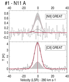
| #1 | 4:57:16.2 | -66:23:20.2 | 2.5 | 139 | N 11 A compact H ii region [CII]+CO peak |
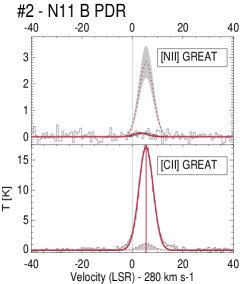
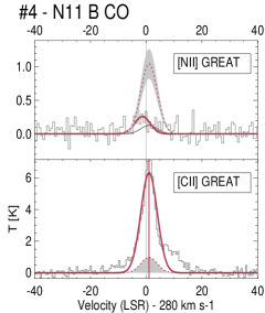
| #2 | 4:56:47.3 | -66:24:30.8 | 2.5 | 143 | N 11 B PDR [C ii] bright |
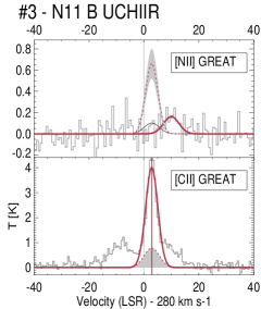
| #3 | 4:56:57.1 | -66:25:12.0 | 5.0 | 101 | N 11 B ultracompact H ii region [C ii] bright |
| #4 | 4:56:55.9 | -66:24:27.7 | 3.1 | 105 | N 11 B center CO peak |
| #5 | 4:56:47.2 | -66:25:09.0 | 14.0 | 60 | N 11 B ionized gas |
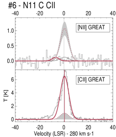
| #6 | 4:57:40.3 | -66:27:06.5 | 3.8 | 92 | N 11 C [C ii] peak |
| #7 | 4:57:42.1 | -66:26:32.2 | 5.0 | 96 | N 11 C CO peak |
| #8 | 4:57:48.4 | -66:28:30.9 | 2.5 | 152 | N 11 C southern [C ii] peak |
| #9 | 4:57:50.6 | -66:29:09.0 | 7.5 | 80 | N 11 D CO peak |
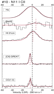
| #10 | 4:55:50.1 | -66:34:35.0 | 5.0 | 90 | N 11 I [C ii] peak |
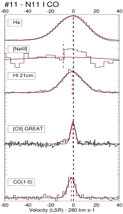
| #11 | 4:55:38.0 | -66:34:18.4 | 2.5 | 126 | N 11 I CO peak |
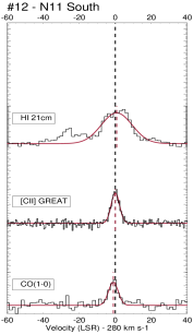
| #12 | 4:56:22.4 | -66:36:56.2 | 2.5 | 136 | N 11 south CO peak |
Most pointings were previously identified as CO-bright peaks in the Magellanic MOPRA Assessment (MAGMA) survey (Wong et al. 2011) or as [C ii] peaks in the Herschel/PACS maps (Fig. 1). A few additional pointings were included, notably toward the young stellar cluster LH 10 in N 11B where the gas is mostly ionized, resulting in bright [O iii] m and m emission (Lebouteiller et al. 2012). Overall, the pointings span various environments including PDRs (e.g., #2), a quiescent CO cloud (#12), an ultracompact H ii region (#3), stellar clusters (#5), among others (Table 2).
The [C ii] line was observed in the GREAT L#2 channel while [N ii] was observed in the L#1 channel. We used X(A)FFT spectrometer back-ends. The [C ii] line was detected toward all pointings. The [N ii] line was observed only toward pointings #1 to #6 but was not detected. Some scans were affected by emission in the offset field111Contamination in the offset was checked during the observations (Sect. 2.1) but only strong contaminations could be identified. for the observation of N 11 I (#11). The chopper amplitude was changed during the observations and the contaminated scans were not used for the final release.
The half power beam width (HPBW) is around for the [C ii] observation and for [N ii]. The exact value of the GREAT HPBW during the observation is unfortunately unknown. We use as a tentative HPBW, following the SOFIA/GREAT Observation Planning (Version 9, April 29, 2016222http://www3.mpifr-bonn.mpg.de/div/submmtech/heterodyne/great/GREAT_calibration.html).
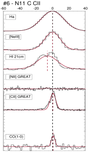
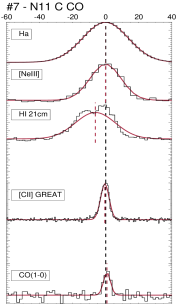
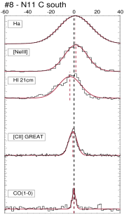
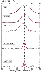
The data were calibrated following Heyminck et al. (2012) and Guan et al. (2012). The reduced spectra shown in this study are in local standard of rest (LSR) velocity (Fig. 2). Spectra were generated from the level 3 GREAT product using the GILDAS/CLASS package. A baseline of first order was subtracted. Calibration from observed counts to main beam temperature was calculated with a beam efficiency for L1 and for L2. The spectral resolution is km s-1 for passband L#2 and km s-1 for L#1, but spectra were rebinned to obtain a channel width of km s-1 to increase the signal-to-noise ratio. For the conversion to Janskys we use the following equation: (GREAT science team; private communication). The flux calibration uncertainty is about (Guan et al. 2012). The final spectra are shown in Figure 2.
2.2 Herschel/PACS
Herschel/PACS observations were taken as part of the SHINING key program (KPGT_esturm_1, PI E. Sturm). Small maps were performed with the unchopped scan mode, for regions LMC-N 11 A, B, C, D, and I in [C ii], [O i] m, and [O iii] m (Cormier et al. 2015). The region N 11 B was also observed in [O i] m, [N ii] m, [N ii] m, and [N iii] m (Lebouteiller et al. 2012). The region N 11 “South” is the only GREAT pointing (#12) with no PACS spectroscopy. All PACS lines appear unresolved given the spectral resolution ( km s-1; Lebouteiller et al. 2012).
The comparison between the [C ii] fluxes measured from GREAT individual pointings and from the PACS map is contingent upon the knowledge of the GREAT beam profile and the flux calibration for both instruments. We use for the GREAT HPBW (see Sect. 2.1). For a Gaussian beam profile, the beam solid angle is then , corresponding to a diameter. Therefore, we convolve the PACS map to a resolution of and integrate the flux in an aperture of diameter. The same steps are performed for the [N ii] observations.
| Pointing | [C ii] | [N ii] m | ||
|---|---|---|---|---|
| W m-2 | W m-2 | |||
| PACS | GREATa | PACS | GREATa | |
| #1 | 1.4 | 2.1 | … | |
| #2 | 3.3 | 5.8 | ||
| #3 | 1.1 | 1.7 | ||
| #4 | 2.2 | 2.7 | ||
| #5 | 0.4 | |||
| #6 | 2.1 | 2.9 | … | |
| #7 | 1.9 | 1.6 | … | … |
| #8 | 2.5 | 4.0 | … | … |
| #9 | 1.0 | … | … | |
| #10 | 0.9 | 1.4 | … | … |
| #11 | 0.5 | 0.9 | … | … |
| #12 | … | 0.6 | … | … |
The fluxes measured with PACS and GREAT are shown in Table 3 for [C ii] and [N ii] m. The agreement is good overall for [C ii], although the PACS fluxes seem to be lower by a factor of on average (see also Fahrion et al. 2017 and Schneider et al. 2018). A better agreement could be reached if the effective GREAT HPBW were somewhat larger ( solid angle). Furthermore, the PACS spectrometer data are calibrated for extended emission, so if the emission is indeed extended, the derived flux will scale with the aperture size; if the emission is point-like however, the total flux of the point source is enclosed in an area somewhat larger than the FWHM of the instrument, and the enclosed energy could be typically underestimated by 444The PACS Spectrometer Calibration Document v3.0 (7-July-2016) http://herschel.esac.esa.int/twiki/bin/view/Public/PacsCalibrationWeb (see also Fahrion et al. 2017).
2.3 H i cm
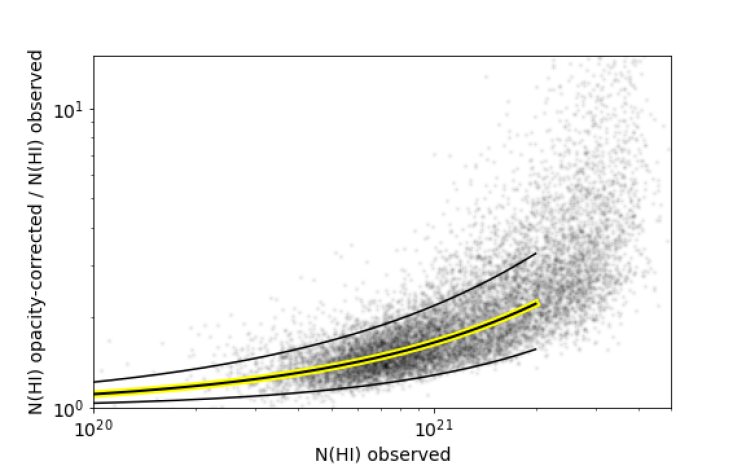
The H i cm data cube is taken from the ATCA+Parkes observations by Kim et al. (2003), which is, at the time of publication, the highest spatial resolution () H i survey of the LMC. The pixel size is and the velocity channels are km s-1. The column density is calculated using a conversion factor for optically thin gas K km s-1 cm-2 (Dickey & Lockman 1990).
Optically thick H i may be significant and an important contributor to the dark neutral medium (DNM) gas as proposed by some authors (e.g., Fukui et al. 2015). We account for optically thick H i by using the results of Braun (2012) for the LMC. The opacity correction is based on a method described in Braun et al. (2009) which computes the temperature as well as the turbulent broadening on scales of pc assuming a spatially resolved isothermal feature (i.e., single temperature along the line of sight). The total column density is then calculated using the profile fit parameters and a correction for the residual emission assumed to be optically thin. To estimate the factor by which we should correct the H0 column density from Kim et al. (2003), we use the smooth variation of the ratio between the velocity-integrated opacity-corrected and -uncorrected (optically thin assumption) H0 column densities. Figure 3 shows this ratio for the N 11 data points. The dispersion in the ratio is partly due to the opacity correction method (e.g., not considering self-absorption) and to the fact that multiple components exist along the line of sight with different opacities. For the H0 column densities measured in individual components (Sect. 4), the correction due to optically thick H i is less than a factor of two (Fig. 3). We consider this correction as an upper limit since other methods to infer the fraction of optically thick H i can result in much lower correction factors (e.g., Lee et al. 2015; Nguyen et al. 2018; Murray et al. 2018).
2.4 CO (1-0)
The CO(1-0) observations are taken from the MAGMA survey described in Wong et al. (2011). Updated reduction is explained in Wong et al. (2017). The original spatial resolution is and we use a pixel size grid. Velocity channels are km s-1. The column density is calculated using a conversion factor555We use the notation to distinguish it from the factor including the CO-dark H2 gas contribution. cm-2 (K km s-1)-1, which is the fiducial value for resolved CO clumps without the contribution of the CO-dark H2 gas between CO clumps as discussed in Roman-Duval et al. (2014). In Table 4 we provide the CO intensity, the H2 column density using , , and the molecular gas fraction defined as (i.e., ignoring the CO-dark H2 gas).
| # | (CO) | |||
|---|---|---|---|---|
| [ cm-2] | [K km s-1] | [ cm-2] | ||
| #1 | ||||
| #2 | ||||
| #3 | ||||
| #4 | ||||
| #5 | ||||
| #6 | ||||
| #7 | ||||
| #8 | ||||
| #9 | ||||
| #10 | ||||
| #11 | ||||
| #12 |
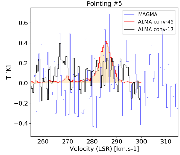
We also obtained ALMA band-3 observations of N 11B (programs 2012.1.00532.S and 2013.1.00556.S; PI Lebouteiller). The mosaic covers the area observed with Herschel/PACS map (Section 2.2). The spatial resolution is ″, with a maximum recoverable scale of ″ and ″ for the - and -m arrays respectively. The velocity resolution is km s-1. The line width ranges between and km s-1. The -m, -m, and Total Power observations were combined for the final data cube. The velocity profiles for the broadest lines are asymmetric, suggesting the presence of multiple components (Fig. 2).
Figure 4 shows the original ALMA map and the projections on the Herschel/PACS [C ii] and MAGMA CO(1-0) grids for comparison. While pointings #2 and #3 coincide well with compact CO peaks observed with ALMA, pointing #4 is somewhat offset by a few arcseconds with respect to the ALMA clump. Given the GREAT beam size (; Sect. 2.1), part of the spatially offset CO cloud emission is expected to contribute to the GREAT pointing #4.
Figure 4 also shows the comparison between MAGMA and ALMA spectra. Overall, there is good agreement between the two datasets over a resolution, with the ALMA spectra showing a drastic S/N improvement. We also show the ALMA spectra calculated for a resolution (i.e., similar to GREAT). On the one hand, ALMA spectra at and resolution are similar for pointing #2, confirming that most of the emission originates from a cloud smaller than with no significant contamination from nearby clouds. On the other hand, the ALMA spectra toward pointings #3 and #4 show some differences with spatial resolution, indicating that nearby clouds with different properties (intensity, central velocity, line width) contribute to the spectrum calculated over a beam for these pointings. Pointing #5 shows no CO emission with ALMA over resolution but emission is seen for the resolution which is likely arising from the main PDR complex corresponding to pointing #2. In the following, the ALMA spectra are used when available in order to compare to the [C ii] spectral profiles. The detailed analysis of the ALMA map is deferred to a future work.
2.5 VLT/GIRAFFE
Optical spectroscopy is used to examine tracers of the ionized gas. We use archival ESO/VLT/U2 GIRAFFE observations with the MEDUSA fiber system feeding component. GIRAFFE is a medium-high () resolution spectrograph in the Å wavelength range. The MEDUSA fibers allow up to separate objects (including sky fibres) to be observed in one go. Each fiber has an aperture of ″on the sky.
The sky-subtracted spectra from program 171.D-0237 were downloaded from the GEPI GIRAFFE archive. We examined in particular H observed with the HR14a grating with ( km s-1), and [Ne iii] Å observed with the HR2 grating with ( km s-1). Some details on the dataset can be found in Torres-Flores et al. (2015).
Most GREAT positions could be associated with a nearby GIRAFFE fiber position, except #12. When several field datasets were available for a given GREAT pointing, we selected only those with the best seeing and S/N. The [Ne iii] and H spectra are shown in Figure 2. The H line is well detected toward all pointings, while [Ne iii] is detected everywhere except in N 11 D and I (GREAT pointings #9 and #10-11 resp.).
3 Integrated properties along the lines of sight
In this section we examine the kinematic properties (radial velocity and line width) integrated along the lines of sight. Results using individual velocity components are discussed in Sect. 4.
3.1 Comparison of the spectral profiles
The CO(1-0) MAGMA spectra can all be fitted reasonably well with a single resolved (i.e., wider than the spectral resolution; Fig. 2) component, with FWHM km s-1 for the lines with the best S/N (see Table 5). The CO(1-0) line was also observed with ALMA in the N 11B region (pointings #2 through #5), which once convolved to resolution shows good agreement with the MAGMA data (Sect. 2.4) but also highlights some asymmetry in the line profile (Fig. 4).
Most [C ii] GREAT spectra can also be fitted with a single resolved component, although a few pointings show evidence of multiple components (most notably #3, #4, #5, #6, and #8) or an asymmetric profile (e.g., #7, #9). The FWHM of [C ii] measured with a single wide component ( km s-1) is always either similar to or larger than the CO FWHM. The H i profile is always much broader than the CO and [C ii] profiles, with FWHM in the range km s-1. Similar results were found in various star-forming regions within nearby galaxies (Braine et al. 2012; de Blok et al. 2016; Requena-Torres et al. 2016; Okada et al. 2015; Fahrion et al. 2017) .
We verified that the difference in the profile line width between H i and CO is not due to the spatial resolution by matching both datasets. However, the wider H i profile as compared to [C ii] is likely driven by the difference in spatial resolution. The H i spectra, taken with resolution (Sect. 2.3), include the emission of clouds outside the GREAT beam. The profile decomposition will allow us to mitigate the biases due to different beam sizes (Sect. 4). Whether from the spectral profiles (Fig. 2) or from the images (Fig. 4), there is no evidence of CO emission not associated with [C ii].
Since [N ii] was not detected with GREAT (Section 2.1), we attempted to use optical tracers (Sect. 2.5) to describe the kinematics of the ionized gas. The observed FWHM of [Ne iii] is km s-1, while it is km s-1 for H. The difference between the two line widths is mostly due to the thermal broadening. The thermal broadening (FWHM) in the ionized gas is
| (1) |
with the temperature and the ionic mass. For a temperature of K (Toribio San Cipriano et al. 2017), we find km s-1 for H+ and km s-1 for Ne2+. Convolutions with the instrumental resolution (Sect. 2.5) and with macro-turbulent motions (typically a few km s-1) yield km s-1 for H and km s-1 for [Ne iii]. Both [Ne iii] and H thus appear somewhat resolved, with a kinematical, nonthermal width of km s-1, which likely reflects the dispersion of several individual components along the line of sight. The only GIRAFFE pointings showing a noticeable velocity structure in [Ne iii] are the ones associated with pointings #2, #4, and #5 in N 11 B. Overall, the spectral resolution in the optical tracers is unfortunately not sufficient to decompose the velocity profiles but the fact that several velocity components may contribute to the observed ionized gas tracer profiles provides a useful constraint for the origin of [C ii] based on its line width (Sect. 3.2.1).
| Pointing | CO | [C ii] | H i | [Ne iii] | H | |||||||||
|---|---|---|---|---|---|---|---|---|---|---|---|---|---|---|
| MAGMA | ALMA; | ALMA; | ||||||||||||
| #1 | … | … | … | … | () | () | ||||||||
| #2 | () | () | () | () | ||||||||||
| #3 | () | () | () | () | ||||||||||
| #4 | () | () | ||||||||||||
| #5 | … | … | … | … | ||||||||||
| … | … | … | … | |||||||||||
| #6 | … | … | … | … | () | () | ||||||||
| #7 | … | … | … | … | () | () | ||||||||
| #8 | … | … | … | … | () | () | ||||||||
| #9 | … | … | … | … | ||||||||||
| #10 | … | … | … | … | ||||||||||
| #11 | … | … | … | … | ||||||||||
| #12 | … | … | … | … | () | () | ||||||||
3.2 Contribution from the ionized gas to [C ii]
The [C ii] line may originate in the neutral (atomic or CO-dark H2) or ionized gas. Unfortunately, no direct comparison of the velocity structure in [C ii] and ionized gas tracers can be performed because the [N ii] m line was not detected with GREAT (Section 2.1) and because the spectral resolution for optical tracers is not high enough (Sect. 3.1).
3.2.1 [C ii] line width
The expected thermal broadening888For a temperature of K (warm neutral medium), the thermal broadening is km s-1, i.e., on the same order as typical macro-turbulence velocity. For the cold neutral medium, macro-turbulence dominates over the thermal broadening. for C+ in the ionized gas is km s-1 (FWHM for a temperature of K). Macro-turbulent motions (typically a few km s-1) may increase this value to km s-1, but we also keep in mind that the temperature in the WIM, where a significant fraction of C+ could exist, may be colder than K. Therefore, we expect [C ii] line widths in the ionized gas for a single velocity component to be in the range km s-1.
The observed FWHM for the main [C ii] velocity component is smaller than km s-1 toward pointings #3, #10, #11, #12, and for one of the two components toward pointing #5 (Table 5). We conclude that [C ii] is necessarily associated with the neutral gas for these components. This conclusion is strengthened if assuming the main [C ii] velocity component in reality corresponds to multiple, narrower components. For some of the other pointings, the [C ii] profile indeed shows multiple blended components (#4, #6) or asymmetric profiles (#7, #8, #9), suggesting that the presence of multiple components drives the large total width (Sect. 3.1). The presence of multiple components in the ionized gas is also suggested by the wide [Ne iii] profiles in the optical (Sect. 3.1).
Pointing #5 is particularly interesting as it shows two well separated [C ii] components, with FWHM of km s-1 and km s-1 for the low- and high-velocity components respectively. While the FWHM of the low-velocity component is compatible with an origin of [C ii] in the neutral gas, the high-velocity component may come from the ionized gas provided it corresponds to a single cloud.
In summary, the observed FWHMs for [C ii], together with the fact that [C ii] in the ionized gas may originate from more than one component, suggests that the observed [C ii] components are unlikely to arise from the ionized gas, except maybe for one component toward pointing #5, and perhaps pointing #1. The line width of all the other [C ii] components is compatible with an origin in the neutral gas, where macro-turbulence competes with the thermal broadening. Other complementary methods are examined in the following.
3.2.2 Ionized gas traced by [N ii] m and m (pointings #1 through #6)
Owing to the energy range required to produce N+ and C+ ions ( eV and eV respectively) and owing to similar critical densities for [C ii] and [N ii] for collisions with , [N ii] lines are often used to trace [C ii] emission in the ionized gas (e.g., Oberst et al. 2006). We can then compare the observed [N ii]/[C ii] ratio to the theoretical value in the ionized gas, with any deviation indicating a contribution from [C ii] in the neutral gas. In order to compute the theoretical ratio, we first calculate the ionic abundance ratio N+/C+ using the solar abundance ratio (Asplund et al. 2009; also valid for LMC-30 Dor Pellegrini et al. 2011) together with the ratio (N+/N) / (C+/C) computed from MAPPINGS III photoionization grids (Sutherland et al. 2013). We then need to account for the gas density. While the m line has a critical density ( cm-3 for collisions with e-) close to that of [C ii] m ( cm-3; Goldsmith et al. 2012), the m line has a larger critical density ( cm-3), meaning that the [N ii] m/[C ii] ratio depends somewhat more on density. Figure 5 shows the theoretical [N ii]/[C ii] ratio as a function of density including the ionic abundance correction factor.
Using the upper limits on the [N ii] m and m lines observed towards N 11B with Herschel/PACS (corresponding to pointings #2, #3, #4, and #5; Sect. 2.2), we find [N ii] m/[C ii] and [N ii] m/[C ii] except toward #5 where [N ii] m/[C ii] (Lebouteiller et al. 2012). The comparison with the theoretical ratio in the ionized gas for typical densities between cm-3 (Fig. 5) indicates that the fraction of velocity-integrated [C ii] originating in the neutral gas is using [N ii] m and using [N ii] m (except for pointing #5 with ). Therefore, for pointings #2, #3, and #4, the fraction of [C ii] in the ionized gas is not significant. For pointing #5 (made of two distinct velocity components), the most stringent constraint is obtained with [N ii] m/[C ii], with for the sum of both components. Since the two [C ii] components toward #5 have similar fluxes, this suggests that the fraction of [C ii] originating in the ionized gas must be relatively small for both. The [N ii] m upper limits calculated from the GREAT spectra (available for #1 through #6) do not allow us to improve further the determination of .
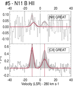
We can also model the velocity profile of [N ii] m with GREAT assuming [C ii] originates fully from the ionized gas and assuming the same velocity structure (i.e., ignoring potential differences in individual component line widths). Our results are illustrated in Figure 6 in which we also show the brightest ionized gas [C ii] emission possible using the [N ii] m upper limits. The density is chosen as cm-3 for this test. It is clear that [C ii] originates overall from the neutral gas. For pointing #5, the simulated [N ii] profile is compatible with the observed profile within uncertainties but we recall that the results using velocity-integrated measurements with Herschel/PACS suggest that the [C ii] contribution from ionized gas is not dominant. We can also conclude that relatively faint [C ii] components observed toward #3, #4, or #6 cannot be explained by [C ii] emission in the ionized gas.
3.2.3 Photoelectric heating efficiency proxy
Finally, the origin of [C ii] can be examined indirectly by comparing the neutral atomic gas cooling traced by the [C ii] and [O i] lines to the gas heating. The latter can be traced by far-infrared emission but contamination by warm dust in the ionized phase can become an issue (Lebouteiller et al. 2012). The PAH emission is another tracer of the neutral gas heating, and it is plausible that PAHs actually dominate the gas heating as compared to very small grains. In LMC-N 11B, Lebouteiller et al. (2012) found that the ratio ([C ii]+[O i])/PAH is uniform, indicating that the photoelectric heating efficiency is fairly constant (see also Helou et al. 2001; Croxall et al. 2012; Okada et al. 2013). The ratio remains constant even toward the stellar cluster LH 10 (corresponding to pointing #5) where ionized gas dominates the infrared line emission, suggesting that [C ii] and [O i] still trace the neutral atomic gas in the foreground and background.
We now revisit this finding by extending the measurement of ([C ii]+[O i])/PAH to all PACS maps in LMC-N 11. Since there is no mid-IR spectra available for all pointings in N 11, we use the IRAC photometry bands to evaluate the PAH emission. We refer to Lebouteiller et al. (2012) for the method. In short, we use the Spitzer/IRAC photometry data points to identify and flag out stellar emission, to estimate and correct for the dust continuum, in order to provide the emission of PAHs either in the IRAC m band (corresponding to the PAH m feature) or in the IRAC m band (corresponding to the PAH m features).
Results are shown in Figure 7, where it can be seen that the cooling rates provided by [C ii] and [O i] compensate, with [C ii] dominating in the faintest, likely more diffuse, regions, and with [O i] dominating in the brightest, more compact, regions. The sum [C ii]+[O i] is however proportional to the PAH emission with no obvious trend with PAH brightness. The remarkably small scatter in ([C ii]+[O i])/PAH in many regions including PDRs (#2) suggests that there is no significant extra [C ii] emission arising from the ionized phase. Potential PAH emission in the ionized gas is ignored as it is plausible that they are photodestroyed (see e.g., Madden et al. 2006; Lebouteiller et al. 2007; Chastenet et al. 2019).
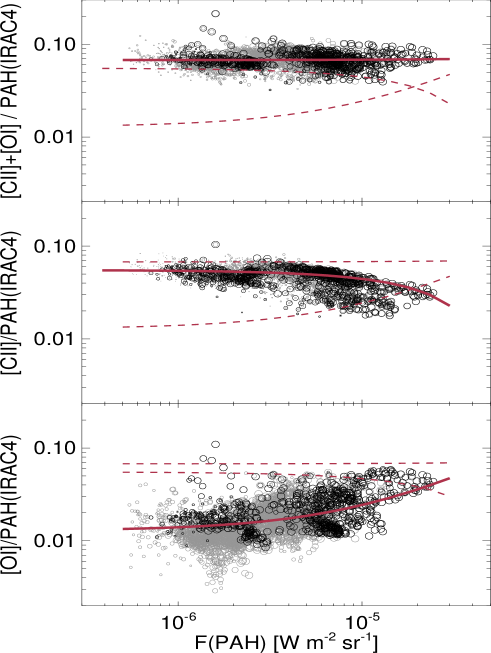
As for the other diagnostics using velocity-integrated values, this result does not preclude the presence of relatively faint [C ii] components that could be associated with the ionized gas. Overall, the results obtained with ([C ii]+[O i])/PAH, together with those obtained in Sections 3.2.1 and 3.2.2, suggest that most of the [C ii] arises in the neutral gas. We find no velocity component that can be unambiguously associated with ionized gas.
4 Individual component analysis
In this section we attempt to decompose the CO, [C ii], and H i profiles toward the GREAT pointings in order to derive the physical conditions associated with each individual component, with the help of simple two-phase models (neutral atomic and molecular). We assume that the ionized contribution to [C ii] is negligible (Sect. 3.2).
4.1 Profile decomposition
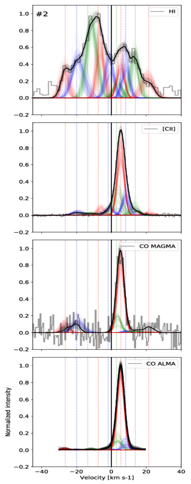
We assume that the velocity structure reflects the presence of several individual components, which we refer to as “clouds”, defined by their radial velocity. We ignore clouds with potentially significant velocity gradient along the line of sight. In other words, all tracers (CO, [C ii], H i) are assumed to peak at the same velocity for any given cloud. Some caveats pertain to the different spatial resolutions of the observations. The H i emission in particular may arise from clouds that are not contributing to the GREAT beam (Sect. 3.1). However, this confusion is mitigated when individual velocity components are considered, since these are more likely to originate from a relatively more spatially confined cloud.
The velocity profiles of CO, [C ii], and H i can be decomposed in various ways, for instance by fitting Gaussian components for the tracer with the narrowest profile, typically CO, and using these centroids for the adjustment of other tracers with other velocity components added as needed (e.g., Okada et al. 2019). We decided to use a statistical approach instead, by adjusting the various profiles simultaneously with velocity components not being fixed or inferred from any other specific profile. Any given component is defined by its velocity and line width, while the component intensity is determined independently for each CO, [C ii], and H i. The sum of the components reproduces the global CO, [C ii], and H i profiles. We also performed decompositions allowing potentially different line widths for each tracer for any given velocity component, but the main results shown in the following remain unchanged.
We use a Bayesian approach with the Markov Chain Monte Carlo (MCMC) PyMC3 code (Salvatier et al. 2016) along with the Metropolis-Hastings sampling algorithm. Parameters are described in Table 6. We identify three parameters that control the number of possible solutions, namely the number of components, the minimum line width, and the minimum separation between components. Although we could narrow down the number of solutions by introducing these parameters within the Bayesian inference (eventually finding a unique converged solution), other degenerate solutions may also be acceptable. Since we consider that we do not have enough observational constraints and priors for these parameters, we chose to test different fixed values:
-
•
The number of components is set to (minimum to reproduce the H i profile) and (to allow potential significant blends).
-
•
The minimum line width is set to and km s-1. The velocity profiles in Figure 2 show that, when the [C ii] profile is visibly made of more than one component (e.g., #3, #4, #6), the [C ii] component associated with CO emission shows the same line width as the CO component, with FWHM values km s-1; Table 5). This suggests that macro-turbulence dominates the [C ii] and CO line width. Therefore, we impose the same line width for a given velocity component in each tracer and ignore line width differences due to mean molecular weight. The lowest value of km s-1 is motivated by the typical turbulence measured for interstellar clouds (e.g., Welty et al. 1994, 1996).
-
•
The minimum component separation is set to km s-1(components with same velocity but potentially different line width), km s-1, and km s-1 (larger values resulting in unsatisfactory fits).
We note that the converged solution for the decomposition, like any other approach, is not claimed to represent the actual velocity structure, but we hope to infer statistically representative trends by making use of the dispersion in the Markov chain (related to flux uncertainties in the spectra), by considering different models (i.e., with different input parameters), and by considering the various pointings. The MCMC method draws a sequence of random variables corresponding to each parameter in the decomposition. Therefore, there are some excursions, especially in the burn-in phase (first iterations, or ”states”, in the chain). Once the burn-in phase is finished, the chain enters a high-probability region where the result has converged. The chain still contains a random distribution though, with excursions according to the uncertainties in the parameter. The standard deviation of the Markov chain therefore provides a probability density function. Figure 8 shows an illustration of the simultaneous fit of all the components. The profile decomposition for the other pointings can be found in Appendix A.
| Parameter | Type | Prior/value |
|---|---|---|
| Number of components () | fixed | |
| Minimum line width () | fixed | km s-1 |
| Minimum separation () | fixed | km s-1 |
| Intensity (Gaussian area) | free, uniform | |
| Line width | free, half-normal | |
| Separation between components | free, half-uniform |
4.2 Model-independent quantities
For each velocity component we compile the [C ii] line intensity, the H0 column density, the H2 column density derived from CO, , and the resulting CO-traced molecular gas fraction . The CO-dark H2 gas will be accounted for later with the model (Sect. 4.3).
We wish to stress that beam dilution may affect H i and CO observations differently if the respective beam filling factors are different. The beam filling factor for CO is likely much smaller than for H i, and as a result the value of should correspond to the beam filling factor of fully molecular clouds embedded in a mostly atomic medium rather than to the actual molecular gas fraction of a single cloud filling the beam.
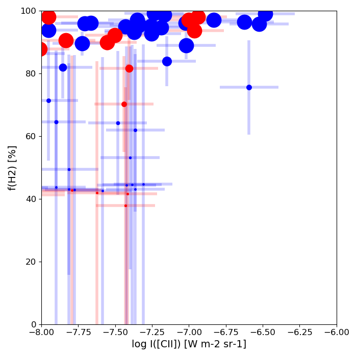
The decomposition results are illustrated in Figure 9, where we show the bivariate kernel density estimate (non-parametric probability density function) of the [C ii] emission and . The kernel density estimation makes use of the data cloud corresponding to every velocity component of every pointing for all the elements in the Markov chain, and for all model input parameters (number of components, minimum component line width, and minimum component separation). Hence the kernel density estimate conveniently indicates whether different solutions to the profile decomposition cluster around similar locii in the parameter space. Most of the components in Figure 9 seem to lie either at or , suggesting a sharp transition between CO-bright H2 gas and either CO-dark H2 or atomic gas. Components with a low are our best candidates for evidence of significant CO-dark H2 gas amount.
4.3 CO-dark gas properties
4.3.1 Selection of components
Our models account for the neutral gas only (atomic and molecular). The ionized gas contribution to the integrated line emission is negligible but its contribution to specific velocity components, in particular faint ones, is more difficult to assess (Sect. 3.2). An upper limit can be calculated for [C ii] in the ionized gas for the pointings with velocity-resolved [N ii] m observations (Sect. 3.2.2; Fig. 6). In the following, we ignore all the [C ii] components below W m-2 sr-1 (corresponding to ) to ensure we select [C ii] components arising in the neutral gas. Although such [C ii] components are faint, and although they do not contribute much to the kernel density estimate plots, we prefer to ignore them for clarity and robustness of the final results. This threshold also prevents over-interpretation of potential [C ii] upper limits corresponding to H i-identified components that do not contribute to the GREAT beam.
4.3.2 Modeling strategy
While the fraction of [C ii] associated with the atomic or molecular phase could be derived from the general profile shapes (e.g., Okada et al. 2019), we choose here a different approach making use of the CO and H0 column densities derived for each velocity component. Since we lack additional constraints (e.g., [O i], [C i], or the infrared luminosity) for the individual velocity components, we cannot derive the physical parameters from PDR models such as the impinging radiation field intensity or the cloud extinction for each individual component. Indirect measurements of such parameters making use of 2D projected quantities are themselves subject to caution (see Seifried et al. 2019 for the extinction). Here we rely on a simple agnostic approach to calculate the level population of C+ accounting for collisions with H0, H2, and as a function of gas temperature and density (see details in Lebouteiller et al. 2013). The clouds that are identified thanks to the velocity decomposition methods are expected to contain both atomic gas, molecular gas traced by CO, and molecular gas traced by C+. For a given velocity component, the CO-dark H2 gas may be related to a CO clump in which case the cloud emits both in [C ii] and CO. The CO-bright H2 gas is not considered in the model because we only calculate the properties of [C ii]-emitting gas, and as such, the H2 column density associated with CO is simply calculated using a fiducial factor (Sect. 2.4).
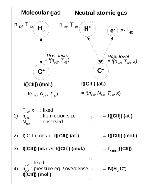
The strategy goes as follows (illustrated in Figure 10):
-
•
Step 1: For each component we calculate a range for the atomic gas number density and the [C ii] emission is estimated in the atomic phase using the atomic gas number density and column density.
-
•
Step 2: The [C ii] intensity from the molecular gas is inferred from the difference of the estimated [C ii] emission in the atomic phase with the observed [C ii].
-
•
Step 3: We compare the [C ii] emission in each phase to compute , which is the fraction of [C ii] associated with gas where collisions with H2 dominate, that is, the CO-dark H2 gas.
-
•
Step 4: From the [C ii] intensity from the molecular gas, we calculate the H2 column density traced by C+, .
For step (1), the number density in the atomic gas is calculated using the H0 column density and assuming that the individual cloud size along the line of sight lies in the range pc999The number density is calculated as , where is the column density and is the cloud size. . Constraints on the cloud size are mostly given by the H i morphology and typical cloud sizes observed with ALMA in 30 Dor (Indebetouw et al. 2013) or N 11 (this study). The inferred density therefore ranges from a few cm-3 to cm-3. The temperature in the atomic phase is fixed assuming that all H i components that can be associated in velocity with [C ii] trace the cold rather than the warm neutral medium (CNM, WNM resp.; see also Pineda et al. 2013, 2017). Accordingly, we estimate a temperature of K from [O i] m/[C ii] (App. C). The resulting pressure is then about K cm-3, which is similar to what is found in predominantly atomic gas within Herschel KINGFISH galaxies (Herrera-Camus et al. 2017) and to other regions in the LMC (Okada et al. 2019) using far-infrared lines. The ionization fraction is fixed to a value of , that is, a typical value for a UV-illuminated diffuse gas in which free electrons are provided by ionization of species with an ionization potential below eV (i.e., no significant ionization from cosmic rays or X-rays).
For step (3), the main free parameter is the H2 column density traced by C+, . We use two constraints for the molecular component: (i) there is no lower limit on the molecular cloud size, but we use the same upper limit as for the atomic gas emission ( pc), and (ii) the number density in the molecular phase scales by default with that in the atomic phase. For the second hypothesis, the scaling assumes by default thermal pressure equilibrium. The expected temperature of the CNM and of the CO-dark H2 gas is about K in Milky Way conditions (Glover & Clark 2016; Tang et al. 2016; Seifried et al. 2019). A somewhat warmer temperature is expected in metal-poor environments due to the larger photoelectric-effect heating efficiency (itself due to the low dust content), to the lack of metal coolants, and to the harder interstellar radiation field (ISRF). We assume in the following a temperature of K in the molecular phase but our results are not changed significantly if we take K. At thermal pressure equilibrium, the density in the H2 gas is therefore twice larger than in the H0 gas, reaching up to cm-3, on the low end of values found in Pineda et al. (2017) for a sample of other LMC star-forming regions. We allow the molecular gas to be denser if no solution can be found with a thermal pressure equilibrium hypothesis. This is motivated by the fact that pressure equilibrium might not always be satisfied (e.g., Vázquez-Semadeni et al. 2000; Scoville 2013) and that thermal pressure may depend on the radiation field intensity and star-formation activity (e.g., Ostriker et al. 2010). Furthermore, the estimated densities correspond to averages along the line of sight while the density structure of the neutral atomic phase and CO-dark H2 gas may differ significantly.
From these results, we can then calculate the following quantities for each velocity component:
-
•
The total H2 column density,
(2) -
•
The fraction of CO-dark H2 gas,
(3) -
•
The mass fraction of molecular gas,
(4)
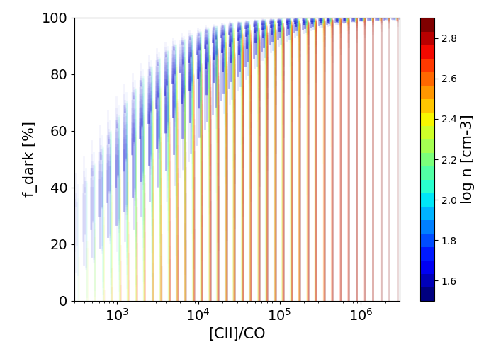
We note that the mass of CO-dark H2 gas we measure is a lower limit because we consider only the gas traced by C+. In principle however, other tracers with possibly different properties may also correspond to CO-dark H2 (Glover & Clark 2016; Clark et al. 2019). In Figure 11 we show the possible model values for as a function of [C ii]/CO for the observed ranges of , , and . The correlation between and [C ii]/CO is tighter for low densities, corresponding to low H0 column densities (due to the assumed cloud size), and therefore to a low fraction of [C ii] in the neutral atomic gas. For such conditions, the [C ii]/CO ratio is proportional to first order101010The tight relationship between and [C ii]/CO is also due to the assumption that the [C ii] and CO emission originate from a single cloud. The global [C ii]/CO ratio measured for a collection of clouds is not a linear function of the ratios in individual clouds. to the column density ratio (e.g., Crawford et al. 1985). As the atomic hydrogen column density increases, so does the possible contribution of the neutral atomic gas to [C ii] (shifting the observed [C ii]/CO to larger values) and so does the number density in the atomic and consequently the molecular gas (leading to lower values). The dependency of with temperature in the atomic gas is relatively small unless the temperature is much larger than K. Even then, if we were to choose a temperature of several thousand K (WNM conditions), values would be lower by less than about % in value.
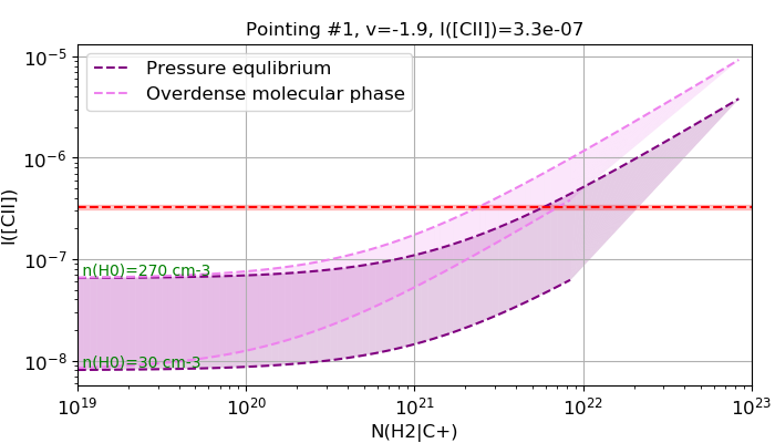
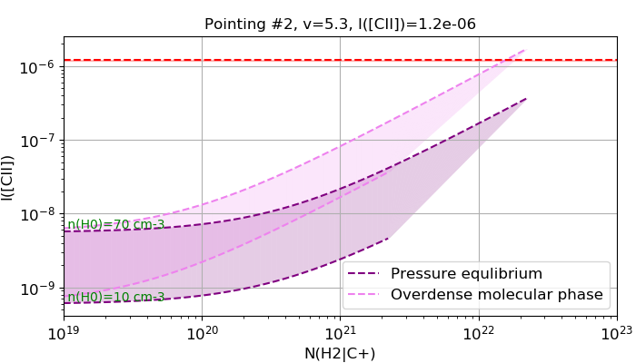
An illustration of the model calculation is shown in Figure 12. In practice, densities in the CO-dark H2 gas lie around cm-3, corresponding to a pressure of K cm-3 (Fig. 13). The total H2 column density measured this way varies across pointings from cm-2 (in #5) to cm-2 (in #10).
4.4 Results
4.4.1 [C ii] in the neutral atomic gas
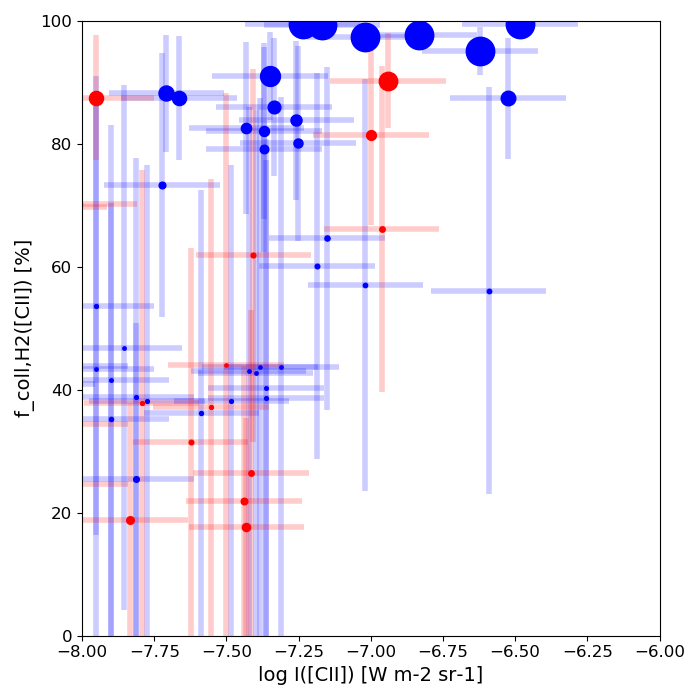
The [C ii] components with low values (Figure 9) could a priori be either from CO-dark H2 gas or atomic gas. When including the contribution from the CO-dark H2 gas calculated by the models, most velocity components reach a large total (including CO-dark H2) molecular gas fraction (Fig. 14), except for the faintest [C ii] components for which only an upper limit on is often available. This indicates that [C ii]-bright regions are dominated by CO-dark H2 gas while [C ii]-faint regions may include a significant contribution from neutral atomic gas.
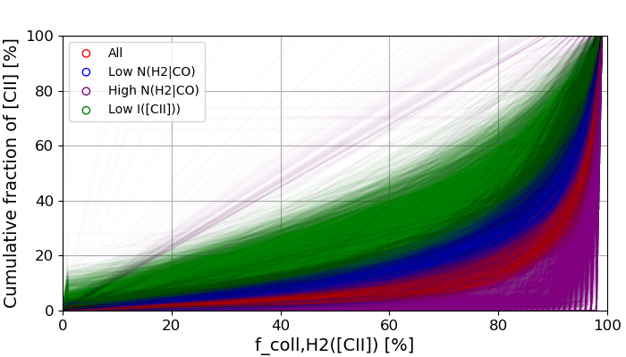
The weak correlation between and in Figure 14 indeed suggests that the contribution of the neutral atomic gas to the [C ii] emission is more significant toward faint [C ii] components, which is confirmed by Figure 25 which shows the distribution of the fraction of [C ii] tracing CO-dark H2 gas, , versus , in particular for #9 and #11.
Figure 15 shows that the [C ii] contribution from the neutral atomic gas does not occur preferentially toward components with low [C ii]/CO. In this figure one can also clearly identify the two components in #5, which are both dominated by CO-dark H2 gas. Most pointings seem to show either a wide distribution of [C ii]/CO values or two main peaks, with the main peak at low [C ii]/CO being due to the velocity component bright in CO and [C ii], while the other peaks with large [C ii]/CO values correspond to [C ii] components with little associated CO emission.
Globally, we find that % of the [C ii] emission across all pointings can be attributed to CO-dark H2 gas (i.e., when ), as shown in Figure 16. This result does not depend on the CO column density and holds in particular for the brightest [C ii] components associated with CO. The [C ii] components that have the largest contribution from the neutral atomic gas (low ), correspond preferentially to the components with the faintest [C ii] surface brightness and not to components with low CO column density (Fig. 16). Even then, less than % of the [C ii] emission in these low-[C ii]-surface-brightness components may be arising from gas that is mostly atomic (i.e., ). Okada et al. (2019) find similar results toward several star-forming regions in the LMC, with of [C ii] being attributed to neutral atomic gas. We wish to emphasize that the larger fraction of [C ii] in the neutral atomic gas in faint [C ii] components is driven by the variation of the [C ii] flux associated with the molecular phase.
In summary, [C ii] mostly traces the CO-dark H2 gas but there is evidence of a weak contribution from the neutral atomic gas in the faintest [C ii] components. The thermal pressure in the CO-dark H2 gas lies around K cm-3 (Fig. 13), which is similar to the range derived by Pineda et al. (2017) for several diffuse (with no CO detection) LMC regions. Considering the large filling factor of [C ii] emission observed in N 11B with Herschel/PACS (Fig. 4), it is therefore plausible that the CO-dark H2 gas probed by our [C ii] observations corresponds to the diffuse ISM (median density cm-3 for all pointings) filling the space between CO clumps rather than thin CO-dark H2 layers around CO clumps.
4.4.2 Fraction of CO-dark H2 gas
We show in Figure 17 the distribution of the fraction of CO-dark H2 gas, , versus [C ii]/CO for each pointing. The fraction of CO-dark H2 gas is also a proxy for the fraction of DNM (i.e., CO-dark H2 gas and optically-thick H i) since the CO-dark H2 gas traced by [C ii] is the main contribution () to the DNM according to our models. The weak contribution of optically thick H i to the DNM is also found in the local and diffuse ISM (Murray et al. 2018; Liszt et al. 2018).
Most pointings show a well-defined peak in Figure 17 corresponding to the brightest [C ii] component. Fainter [C ii] components often result in a wide range of values because they are more likely to arise from the neutral atomic phase (with relatively large uncertainty; Sect. 4.4.1). From Figure 17 we see that most of the molecular gas is CO-dark overall, with . Since most of the molecular gas is CO-dark, we conclude that the velocity-integrated ([C ii]+[O i])/PAH ratio, which suggests a constant photoelectric-effect heating efficiency across N 11 (Sect. 3.2.3), corresponds in fact to the physical conditions of the CO-dark H2 gas rather than the neutral atomic medium.
The values we find are in good agreement with the estimates of Galametz et al. (2016) in N 11 using the dust-to-gas mass ratio. Our results are also in general agreement with other studies in nearby low-metallicity environments. Fahrion et al. (2017) used SOFIA/GREAT observations the dwarf galaxy NGC 4214 at pc spatial scale and found that only % of [C ii] could be attributed to the CNM and that % of the H2 mass is not traced by CO. Other studies in the Magellanic Clouds also show significant CO-dark H2 gas fractions. Requena-Torres et al. (2016) examined several star-forming regions in the SMC, and found that most of the [C ii] emission originates from CO-dark H2 gas. Chevance (2016) observed LMC-30 Dor and determined from PDR models that % of the molecular gas is CO-dark H2 gas.
In N 11, there is a clear correlation between and [C ii]/CO (Fig. 17), which is not surprising because the CO-dark H2 gas in the model is by construction traced by C+ and because the contribution of [C ii] in the neutral atomic gas is relatively small (Sect. 4.3.2). For this reason, the [C ii]/CO ratio we use in Figure 17 is the observed value, i.e., with no correction for the [C ii] in the atomic gas. For a given [C ii]/CO ratio, the range of values is driven by the H0 column density which sets the density in the atomic gas and consequently in the molecular gas (Sect. 4.3.2).
Most points seem to follow the same relationship between and [C ii]/CO (dashed curve in Fig. 17). For [C ii]/CO, this is because depends little on the gas density (Sect. 4.3.2). For lower [C ii]/CO values, depends more on density and components with similar [C ii]/CO ratios may have significantly different values (e.g., from for #9 to for #5).
We also find that is anti-correlated with the CO column density (Fig. 18). Most of the molecular gas is therefore CO-dark, but there is more CO-dark gas in CO-faint regions (% for cm-2) as compared to CO peaks (% for cm-2). This result is reminiscent of the findings of Okada et al. (2015) that the amount of [C ii] that cannot be attributed to the gas traced by CO is larger between CO peaks in another LMC star-forming region, N 159.
4.4.3 Physical parameters controlling
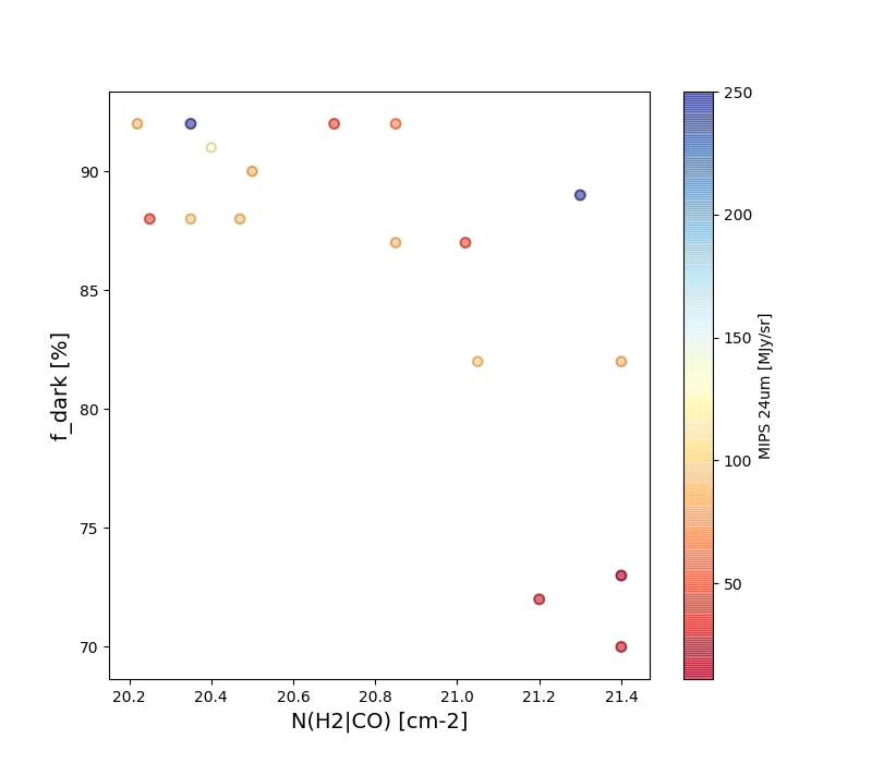
We find that is somewhat larger for components with a large [C ii]/CO ratio (Fig. 17), which should correspond to molecular clouds illuminated by the UV radiation from massive stars, providing some evidence that stellar feedback may play a role. In Figure 18, the pointings are ordered based on the shape of the with distribution, from pointings with a high and almost flat distribution until column densities of cm-2 to pointings showing a steep decrease of for column densities above cm-2. The difference between the various pointings is most pronounced for large column densities cm-2. We note that the larger values are not a direct consequence of the fact that a relatively dense molecular phase might be required, since in such cases a somewhat lower column density of CO-dark H2 gas will be determined (Fig. 10). Interestingly, the sequence of pointings in Figure 18 also correlates with the presence of bright H and m emission near molecular clouds (Fig. 1). For instance pointings #9, #11, and #12 show particularly low values and high CO column densities and they are also the pointings with the faintest H (or m) emission. This result is also shown in Figure 19 where we report the m emission for each peak in the distribution of each pointing.
Stellar feedback could have an impact on the fraction of CO-dark H2 gas, either through intense radiation field (ionization, radiation pressure) or through dynamical/mechanical effects from winds and supernovae shocks resulting in disruption/dispersal of molecular clouds (e.g., Dale et al. 2012) and therefore to a lower beam-averaged extinction . The average extinction toward a given pointing is driven by the selective disruption and photodissociation of the most diffuse clouds (thereby selecting out the clouds with the highest extinction) and the overall eroding of all clouds. From a theoretical perspective, Wolfire et al. (2010) find that for fixed the fraction of CO-dark H2 gas in a molecular cloud is insensitive to the incident radiation field, although with the latter not exceeding times the local Galactic radiation field. In contrast, these latter authors find that increases with decreasing . On the other hand, kiloparsec-scale simulations of spiral galaxies show that is a function of the radiation field and of the surface density (Smith et al. 2014). Fahrion et al. (2017) modeled the star-forming dwarf galaxy NGC 4214 and found that the fraction of CO-dark H2 gas mass depends on the evolutionary stage of the star-forming regions, with a larger fraction towards the naked cluster as compared to compact embedded regions. Madden et al. (in preparation) modeled PDRs in galaxies from the Herschel Dwarf Galaxy Survey (DGS) and find that the effective extinction derived in the model is the main parameter controlling .
Unfortunately, our models do not allow us to directly examine parameters such as or the radiation field strength , for lack of other transitions or dust measurements corresponding to individual velocity components, but we may hope to disentangle both parameters from or [C ii]/CO. Since is proportional to the CO intensity which correlates with extinction on parsec scales (Lee et al. 2018), the trends in Figure 18 can be understood to first order as the variations of with for a single cloud hypothesis. With this in mind, the decrease of for cm-2 would be due to the increase of CO column density with the cloud size while the mass in the CO-dark H2 gas layer saturates, and should then be the main parameter controlling . However, the fact that we observe different values for a given value implies either that a parameter other than controls (a parameter correlating with [C ii]/CO since correlates best with [C ii]/CO; Fig. 17) or that does not accurately trace (for instance because our observations combine multiple clouds).
4.5 Influence of metallicity
In this section we apply our models to the data from Pineda et al. (2017) for LMC and SMC pointings (lines of sight toward H i-bright, CO-bright, and/or m-bright regions). The SMC data points are useful probes of a lower-metallicity environment ( Z⊙) as compared to the LMC ( Z⊙). The spectral profiles of H i and CO were used in Pineda et al. (2017) but individual velocity components were not adjusted to mitigate the different angular resolution in each tracer. We use the H i CNM value (integrated over the [C ii] line FWHM) in Pineda et al. (2017). For our models, the CO-to-H2 conversion factor for the SMC is taken as cm-2 (K km s-1)-1 (Roman-Duval et al. 2014). We selected data points with detections in H i, [C ii], and CO, and with W m-2 sr-1 in order to be coherent with the present study (Sect. 4.3.1).
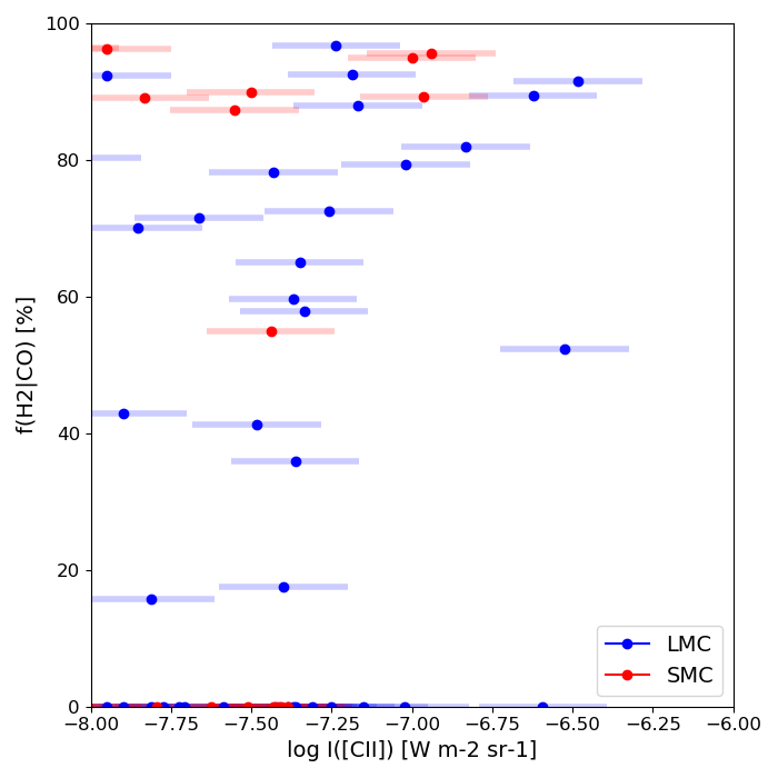
Results are shown in Figure 20. Overall, the results agree with our study for LMC data points, that is, bright [C ii] components have a molecular gas fraction near unity, the contribution of neutral atomic gas to the [C ii] emission is larger for faint [C ii] components ( W m-2 sr-1), and the fraction of CO-dark H2 gas decreases with the CO column density. The comparison with our results illustrates some advantages related to the profile decomposition. First, while our study was performed with fewer pointings, by accounting for multiple velocity components corresponding to various physical conditions, statistically significant results could be obtained. Furthermore, we were able to some extent to probe components with large [C ii]/CO values which may correspond to relatively quiescent clouds (Fig. 17).
Toward SMC regions, the fraction of [C ii] emission corresponding to CO-dark H2 gas, , is somewhat lower, while is somewhat larger for a given CO column density as compared to the LMC. In other words, more [C ii] can be explained by atomic gas in the SMC, but the fraction of CO-dark H2 gas is larger. It is possible that the larger values obtained for the SMC are related to a larger incident radiation field but it is also possible that the gas temperature we assume for the SMC (the same as for the LMC) is not applicable. As noted by Glover & Clark (2016), the detectability of the CO-dark H2 gas with [C ii] or [O i] in fact improves greatly with the ISRF strength (which increases the photoelectric-effect heating rate and hence the gas temperature). While we have chosen the same temperatures for the LMC and SMC regions, in the SMC would be compatible with the LMC values if the temperature was scaled up by a factor of only two to four. Results for the DGS using integrated measurements show that there is no simple relationship between metallicity and and that the latter mostly depends on extinction (Madden et al. in prep.).
5 Conclusions
We present a study of the CO-dark H2 gas in the giant H ii region N 11 in the LMC, with a half-solar metallicity. Twelve pointings were observed with SOFIA/GREAT in [C ii]. The [C ii] velocity profile is compared to that of CO(1-0) observed with MOPRA and ALMA, and to that of H i observed with ATCA+Parkes. The objectives are to measure the total molecular gas content, the fraction of CO-dark H2 gas, and to probe the influence of the environment (in particular stellar feedback). First we investigated velocity-integrated properties. The main results obtained are as follows.
-
•
The [C ii] emission originates mostly from the neutral gas, except for one velocity component toward one of the pointings (#5) for which the result is unclear. This result is found through various methods using the [C ii] line width, the [N ii]/[C ii] ratio in the ionized gas, the [N ii] m velocity profile observed with GREAT, and the photoelectric-effect heating efficiency proxy ([C ii]+[O i])/PAH.
-
•
The photoelectric-effect heating efficiency proxy ([C ii]+[O i])/PAH is found to be constant throughout the regions in N 11 observed with Herschel/PACS, generalizing somewhat the results previously obtained in N 11B by Lebouteiller et al. (2012) that the sum [C ii]+[O i] traces the total cooling, that PAH emission traces the gas heating, and that [C ii] mostly originates from the neutral gas. Our results suggest that this gas is CO-dark H2 and not atomic.
-
•
The total profile width of [C ii] is found to be between that of CO(1-0) and H i, but the [C ii] profile resembles more that of CO(1-0).
We then decomposed the profiles using a Bayesian method and a statistical approach that makes use of the many pointings together with a range of input parameters concerning the number of velocity components, the minimum individual component line width, and the minimum separation between components. A simple model was used to compute the [C ii] line intensity accounting for collisions with H0, H2, and in a two-phase medium (neutral atomic and molecular) as a function of gas temperature and density. The main results obtained are as follows:
-
•
The variations of are driven by the [C ii] emission in the molecular phase. As a result, the [C ii] components with the largest contribution from H0 gas are preferentially those with a low [C ii] surface brightness rather than those with low [C ii]/CO or low CO column density. However, the contribution from H0 gas to [C ii] is never dominant.
-
•
There is a sharp transition between CO-bright and CO-dark H2 gas, with the latter quickly becoming the dominant H2 reservoir.
-
•
Overall (combining all pointings and all velocity components), more than % of the [C ii] emission arises in the (CO-dark) H2 gas.
-
•
Most of the molecular gas is CO-dark (fraction between and %), in particular toward the brightest [C ii] components.
-
•
The CO-dark H2 gas traced by [C ii] is rather diffuse with cm-3 on average for all pointings. We identify in particular a specific [C ii] velocity component toward #5 with a density around cm-3.
-
•
The contribution of optically thick H i to the dark neutral medium is not significant.
-
•
Most components follow the same trend of the fraction of CO-dark H2 versus [C ii]/CO, with some deviations driven by the gas density.
-
•
The effective factor including the CO-dark H2 gas lies in the range (K km s-1)-1 for most of the bright velocity components.
-
•
The fraction of CO-dark H2 gas decreases with increasing CO column density, but while it is rather constant for CO column density cm-2, it shows a large dispersion above this value. We argue that, for a given CO column density, the larger fractions of CO-dark H2 gas are found toward CO clouds at the interface with H-bright regions. It is plausible that stellar feedback (either through radiation or dynamical/mechanical effects from stellar winds and supernovae shocks) results in the disruption and dispersal of molecular clouds and in turn a lower extinction on average.
-
•
Our simple models were applied to the LMC and SMC pointings in Pineda et al. (2017). We find circumstancial evidence that the fraction of CO-dark H2 gas is larger for a given CO column density in the SMC as compared to the LMC, but this conclusion is weakened by the uncertain gas temperature.
The main caveat concerns the derived column density and number density in the atomic medium, with limited spatial resolution, even though the velocity decomposition somewhat mitigates the correspondence between components in the different tracers. Further observations at larger spatial resolution in H i would greatly improve our knowledge of the origin of [C ii] and its performance as a CO-dark H2 gas tracer. Moreover, observations of [O i] would shed light on the physical conditions of the few components where [C ii] arises in the neutral atomic medium. In particular, more constraints are needed to examine the incident radiation field and extinction in individual clouds, which would then help the understanding of the nature of stellar feedback responsible for the variations of the fraction of CO-dark H2 gas. Finally, we are aware that the assumption that the velocity components from different tracers arise from a given cloud is increasingly problematic at increasingly large scales, but we cannot unfortunately thoroughly test this hypothesis with the present dataset.
Acknowledgements.
Based on observations made with the NASA/DLR Stratospheric Observatory for Infrared Astronomy (SOFIA). SOFIA is jointly operated by the Universities Space Research Association, Inc. (USRA), under NASA contract NAS2-97001, and the Deutsches SOFIA Institut (DSI) under DLR contract 50 OK 0901 to the University of Stuttgart. This paper makes use of the following ALMA data: ADS/JAO.ALMA#2012.1.00532.S and ADS/JAO.ALMA#2013.1.00556.S. ALMA is a partnership of ESO (representing its member states), NSF (USA) and NINS (Japan), together with NRC (Canada) and NSC and ASIAA (Taiwan) and KASI (Republic of Korea), in cooperation with the Republic of Chile. The Joint ALMA Observatory is operated by ESO, AUI/NRAO and NAOJ. V. Lebouteiller wishes to thank S. Kannappan and C. Iliadis for making it possible to do part of this work at UNC Chapel Hill. MC gratefully acknowledges funding from the Deutsche Forschungsgemeinschaft (DFG) through an Emmy Noether Research Group, grant number KR4801/1-1. M.-Y.L. was partially funded through the sub-project A6 of the Collaborative Research Council 956, funded by the Deutsche Forschungsgemeinschaft (DFG). DC is supported by the European Union’s Horizon 2020 research and innovation programme under the Marie Skłodowska-Curie grant agreement No 702622. FLP is supported by the ANR grant LYRICS (ANR-16-CE31-0011). This work was supported by the Programme National “Physique et Chimie du Milieu Interstellaire” (PCMI) of CNRS/INSU with INC/INP co-funded by CEA and CNES.References
- Aravena et al. (2016) Aravena, M., Decarli, R., Walter, F., et al. 2016, ApJ, 833, 71
- Asplund et al. (2009) Asplund, M., Grevesse, N., Sauval, A. J., & Scott, P. 2009, ARA&A, 47, 481
- Braine et al. (2012) Braine, J., Gratier, P., Kramer, C., et al. 2012, A&A, 544, A55
- Braun (2012) Braun, R. 2012, ApJ, 749, 87
- Braun et al. (2009) Braun, R., Thilker, D. A., Walterbos, R. A. M., & Corbelli, E. 2009, ApJ, 695, 937
- Chastenet et al. (2019) Chastenet, J., Sandstrom, K., Chiang, I. D., et al. 2019, ApJ, 876, 62
- Chevance (2016) Chevance, M. 2016, PhD thesis, Université Sorbonne Paris Cité - Université Paris.Diderot
- Chevance et al. (2016) Chevance, M., Madden, S. C., Lebouteiller, V., et al. 2016, A&A, 590, A36
- Clark et al. (2019) Clark, P. C., Glover, S. C. O., Ragan, S. E., & Duarte-Cabral, A. 2019, MNRAS, 486, 4622
- Cormier et al. (2015) Cormier, D., Madden, S. C., Lebouteiller, V., et al. 2015, A&A, 578, A53
- Crawford et al. (1985) Crawford, M. K., Genzel, R., Townes, C. H., & Watson, D. M. 1985, ApJ, 291, 755
- Croxall et al. (2012) Croxall, K. V., Smith, J. D., Wolfire, M. G., et al. 2012, ApJ, 747, 81
- Dale et al. (2012) Dale, J. E., Ercolano, B., & Bonnell, I. A. 2012, MNRAS, 424, 377
- de Blok et al. (2016) de Blok, W. J. G., Walter, F., Smith, J.-D. T., et al. 2016, AJ, 152, 51
- De Looze et al. (2014) De Looze, I., Cormier, D., Lebouteiller, V., et al. 2014, A&A, 568, A62
- Dickey & Lockman (1990) Dickey, J. M. & Lockman, F. J. 1990, ARA&A, 28, 215
- Fahrion et al. (2017) Fahrion, K., Cormier, D., Bigiel, F., et al. 2017, A&A, 599, A9
- Franeck et al. (2018) Franeck, A., Walch, S., Seifried, D., et al. 2018, MNRAS[arXiv:1809.10696]
- Fukui et al. (2015) Fukui, Y., Torii, K., Onishi, T., et al. 2015, ApJ, 798, 6
- Galametz et al. (2016) Galametz, M., Hony, S., Albrecht, M., et al. 2016, MNRAS, 456, 1767
- Galliano et al. (2011) Galliano, F., Hony, S., Bernard, J.-P., et al. 2011, A&A, 536, A88
- Glover & Clark (2016) Glover, S. C. O. & Clark, P. C. 2016, MNRAS, 456, 3596
- Goldsmith et al. (2012) Goldsmith, P. F., Langer, W. D., Pineda, J. L., & Velusamy, T. 2012, ApJS, 203, 13
- Grenier et al. (2005) Grenier, I. A., Casandjian, J.-M., & Terrier, R. 2005, Science, 307, 1292
- Guan et al. (2012) Guan, X., Stutzki, J., Graf, U. U., et al. 2012, A&A, 542, L4
- Helou et al. (2001) Helou, G., Malhotra, S., Hollenbach, D. J., Dale, D. A., & Contursi, A. 2001, ApJ, 548, L73
- Herrera et al. (2013) Herrera, C. N., Rubio, M., Bolatto, A. D., et al. 2013, A&A, 554, A91
- Herrera-Camus et al. (2017) Herrera-Camus, R., Bolatto, A., Wolfire, M., et al. 2017, ApJ, 835, 201
- Heyminck et al. (2012) Heyminck, S., Graf, U. U., Güsten, R., et al. 2012, A&A, 542, L1
- Indebetouw et al. (2013) Indebetouw, R., Brogan, C., Chen, C.-H. R., et al. 2013, ApJ, 774, 73
- Israel (1997) Israel, F. P. 1997, A&A, 328, 471
- Israel et al. (2003) Israel, F. P., de Graauw, T., Johansson, L. E. B., et al. 2003, A&A, 401, 99
- Israel & Maloney (2011) Israel, F. P. & Maloney, P. R. 2011, A&A, 531, A19
- Jameson et al. (2018) Jameson, K. E., Bolatto, A. D., Wolfire, M., et al. 2018, ApJ, 853, 111
- Kim et al. (2003) Kim, S., Staveley-Smith, L., Dopita, M. A., et al. 2003, ApJS, 148, 473
- Langer et al. (2014) Langer, W. D., Velusamy, T., Pineda, J. L., Willacy, K., & Goldsmith, P. F. 2014, A&A, 561, A122
- Lebouteiller et al. (2007) Lebouteiller, V., Brandl, B., Bernard-Salas, J., Devost, D., & Houck, J. R. 2007, ApJ, 665, 390
- Lebouteiller et al. (2012) Lebouteiller, V., Cormier, D., Madden, S. C., et al. 2012, A&A, 548, A91
- Lebouteiller et al. (2013) Lebouteiller, V., Heap, S., Hubeny, I., & Kunth, D. 2013, A&A, 553, A16
- Lee et al. (2018) Lee, C., Leroy, A. K., Bolatto, A. D., et al. 2018, MNRAS, 474, 4672
- Lee et al. (2015) Lee, M.-Y., Stanimirović, S., Murray, C. E., Heiles, C., & Miller, J. 2015, ApJ, 809, 56
- Liszt et al. (2018) Liszt, H., Gerin, M., & Grenier, I. 2018, A&A, 617, A54
- Madden & Cormier (2018) Madden, S. C. & Cormier, D. 2018, arXiv e-prints, arXiv:1810.09953
- Madden et al. (2006) Madden, S. C., Galliano, F., Jones, A. P., & Sauvage, M. 2006, A&A, 446, 877
- Madden et al. (1997) Madden, S. C., Poglitsch, A., Geis, N., Stacey, G. J., & Townes, C. H. 1997, ApJ, 483, 200
- Madden et al. (2013) Madden, S. C., Rémy-Ruyer, A., Galametz, M., et al. 2013, PASP, 125, 600
- Mookerjea et al. (2016) Mookerjea, B., Israel, F., Kramer, C., et al. 2016, A&A, 586, A37
- Murray et al. (2018) Murray, C. E., Peek, J. E. G., Lee, M.-Y., & Stanimirović, S. 2018, ApJ, 862, 131
- Nguyen et al. (2018) Nguyen, H., Dawson, J. R., Miville-Deschênes, M.-A., et al. 2018, ApJ, 862, 49
- Oberst et al. (2006) Oberst, T. E., Parshley, S. C., Stacey, G. J., et al. 2006, ApJ, 652, L125
- Okada et al. (2019) Okada, Y., Güsten, R., Requena-Torres, M. A., et al. 2019, A&A, 621, A62
- Okada et al. (2013) Okada, Y., Pilleri, P., Berné, O., et al. 2013, A&A, 553, A2
- Okada et al. (2015) Okada, Y., Requena-Torres, M. A., Güsten, R., et al. 2015, A&A, 580, A54
- Ostriker et al. (2010) Ostriker, E. C., McKee, C. F., & Leroy, A. K. 2010, ApJ, 721, 975
- Pellegrini et al. (2011) Pellegrini, E. W., Baldwin, J. A., & Ferland, G. J. 2011, ApJ, 738, 34
- Pérez-Beaupuits et al. (2015) Pérez-Beaupuits, J. P., Stutzki, J., Ossenkopf, V., et al. 2015, A&A, 575, A9
- Pineda et al. (2014) Pineda, J. L., Langer, W. D., & Goldsmith, P. F. 2014, A&A, 570, A121
- Pineda et al. (2017) Pineda, J. L., Langer, W. D., Goldsmith, P. F., et al. 2017, ApJ, 839, 107
- Pineda et al. (2013) Pineda, J. L., Langer, W. D., Velusamy, T., & Goldsmith, P. F. 2013, A&A, 554, A103
- Polles et al. (2019) Polles, F. L., Madden, S. C., Lebouteiller, V., et al. 2019, A&A, 622, A119
- Requena-Torres et al. (2016) Requena-Torres, M. A., Israel, F. P., Okada, Y., et al. 2016, A&A, 589, A28
- Roman-Duval et al. (2014) Roman-Duval, J., Gordon, K. D., Meixner, M., et al. 2014, ApJ, 797, 86
- Salvatier et al. (2016) Salvatier, J., Wiecki, T. V., & Fonnesbeck, C. 2016, PeerJ Computer Science, 2, e55
- Schneider et al. (2018) Schneider, F. R. N., Sana, H., Evans, C. J., et al. 2018, Science, 359, 69
- Scoville (2013) Scoville, N. Z. 2013, Evolution of star formation and gas (Falcón-Barroso, J. and Knapen, J. H.), 491
- Seifried et al. (2019) Seifried, D., Haid, S., Walch, S., Borchert, E. M., & Bisbas, T. G. 2019, arXiv e-prints, arXiv:1906.01015
- Smith et al. (2014) Smith, R. J., Glover, S. C. O., Clark, P. C., Klessen, R. S., & Springel, V. 2014, MNRAS, 441, 1628
- Sutherland et al. (2013) Sutherland, R., Dopita, M., Binette, L., & Groves, B. 2013, MAPPINGS III: Modelling And Prediction in PhotoIonized Nebulae and Gasdynamical Shocks, Astrophysics Source Code Library
- Tang et al. (2016) Tang, N., Li, D., Heiles, C., et al. 2016, A&A, 593, A42
- Toribio San Cipriano et al. (2017) Toribio San Cipriano, L., Domínguez-Guzmán, G., Esteban, C., et al. 2017, MNRAS, 467, 3759
- Torres-Flores et al. (2015) Torres-Flores, S., Barbá, R., Maíz Apellániz, J., Rubio, M., & Bosch, G. 2015, in IAU Symposium, Vol. 309, Galaxies in 3D across the Universe, ed. B. L. Ziegler, F. Combes, H. Dannerbauer, & M. Verdugo, 153–154
- Vázquez-Semadeni et al. (2000) Vázquez-Semadeni, E., Gazol, A., & Scalo, J. 2000, ApJ, 540, 271
- Welty et al. (1994) Welty, D. E., Hobbs, L. M., & Kulkarni, V. P. 1994, ApJ, 436, 152
- Welty et al. (1996) Welty, D. E., Morton, D. C., & Hobbs, L. M. 1996, ApJS, 106, 533
- Wolfire et al. (2010) Wolfire, M. G., Hollenbach, D., & McKee, C. F. 2010, ApJ, 716, 1191
- Wong et al. (2011) Wong, T., Hughes, A., Ott, J., et al. 2011, ApJS, 197, 16
- Wong et al. (2017) Wong, T., Hughes, A., Tokuda, K., et al. 2017, ApJ, 850, 139
- Young et al. (2012) Young, E. T., Becklin, E. E., Marcum, P. M., et al. 2012, ApJ, 749, L17
Appendix A Profile decomposition for each pointing
The spectral decomposition of the H i CO, and [C ii] spectra obtained for the GREAT pointings is shown in Figures 21, 22, 23, 24. The decomposition is only shown for the model with ten components, a minimum line width of km s-1, and a minimum component separation of km s-1.
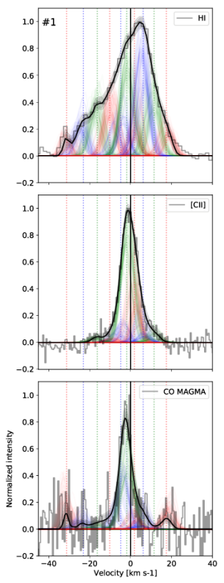

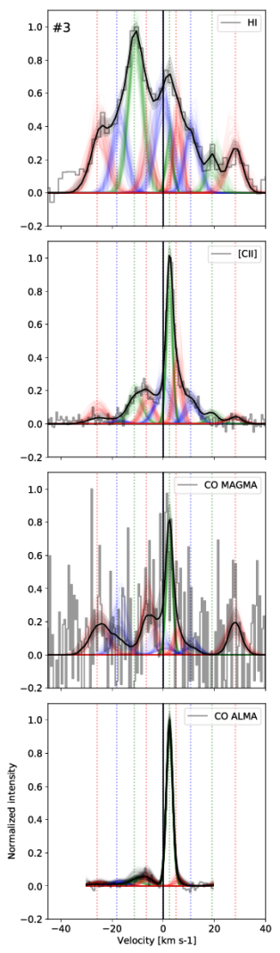
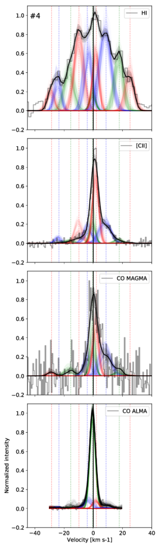
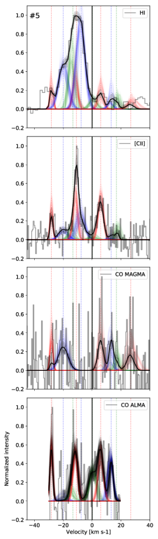
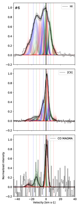
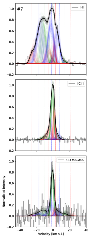
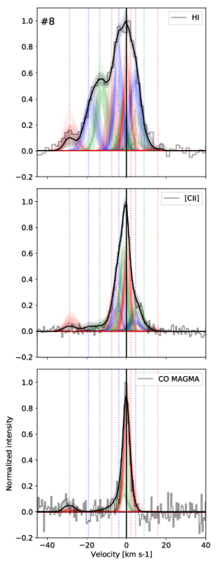
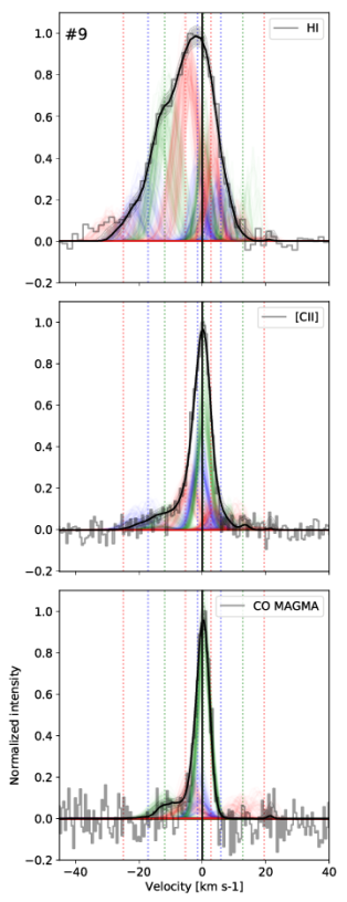
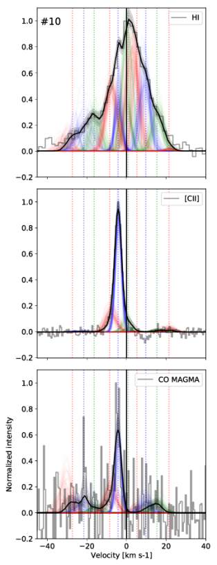
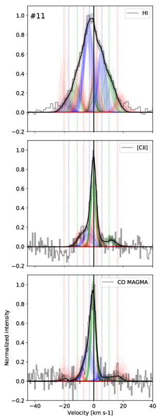
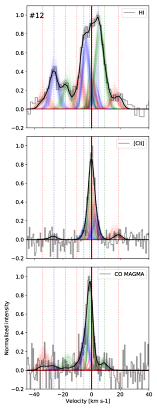
Appendix B Kernel density estimates
The kernel density estimate of the fraction of [C ii] tracing CO-dark H2 gas, , and is shown in Figure 25. The distribution is globally similar to that of versus (Fig. 14) because most H2 is CO-dark and because the CO-dark H2 gas is traced by [C ii].
Figure 26 shows the kernel density estimate of the effective conversion factor and the [C ii]/CO ratio. Since the conversion factor includes the contribution of the CO-dark H2 gas, it is larger than the fiducial value cm-2 (K km s-1)-1 (Sect. 2.4). We find an effective in the range (K km s-1)-1 for most of the bright velocity components, in good agreement with values obtained in Israel (1997); Galliano et al. (2011); Chevance (2016).
Appendix C Gas temperature determination
The temperature in the neutral atomic gas can in principle be estimated from the [O i] m/[C ii] ratio observed with Herschel/PACS (Lebouteiller et al. 2012). Apart from optical depth effects for the [O i] m line (see Lebouteiller et al. 2012), another problem resides in the fact that [C ii], and presumably [O i], mostly trace the molecular phase rather than the neutral atomic phase, as our present results suggest. For this reason we use the extended emission seen in the PACS maps and assume it to be dominated by atomic gas. For extended emission, the [O i] m/[C ii] ratio is in the range (Fig. 27 left), corresponding to a temperature of a few hundred Kelvin for densities cm-3 (Fig. 27 right), while somewhat lower temperature values would be found if the medium were partly molecular.