References
- [1]
- [2]
- [3]
- [4] \makeframing
Probing the robustness of nested multi-layer networks
Abstract
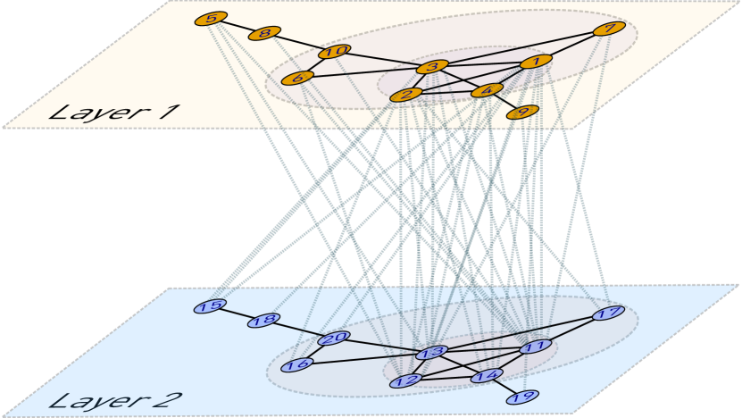
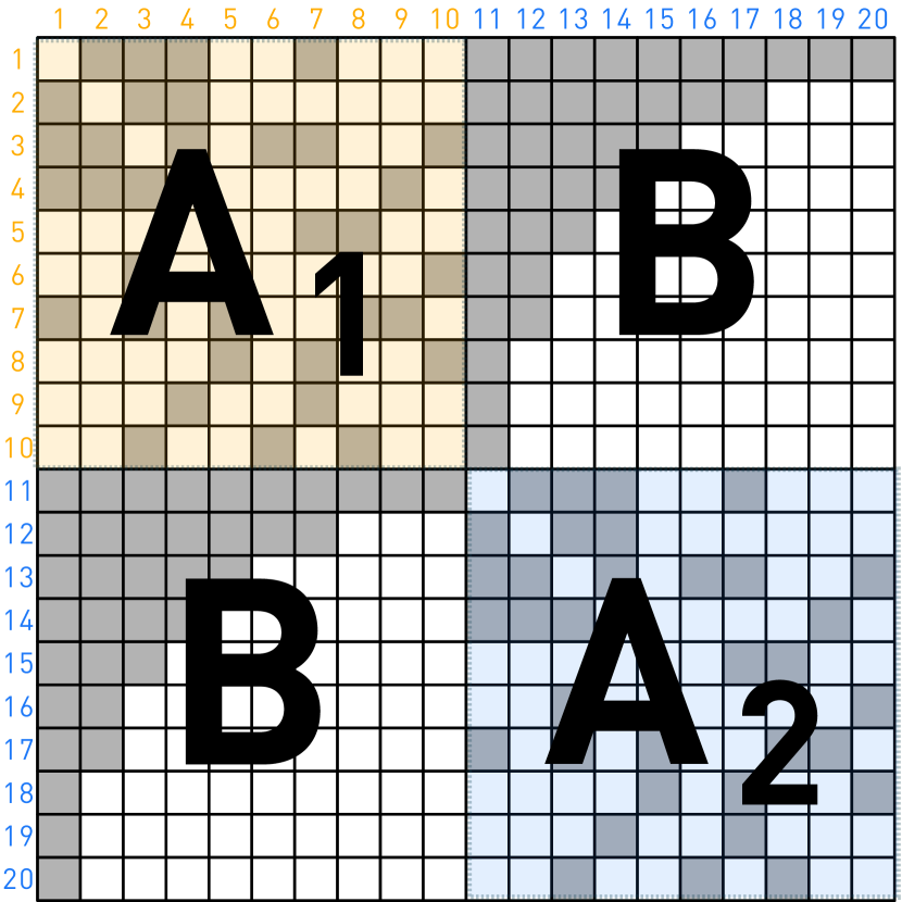
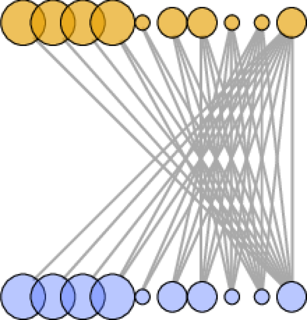
We consider a multi-layer network with two layers, , .
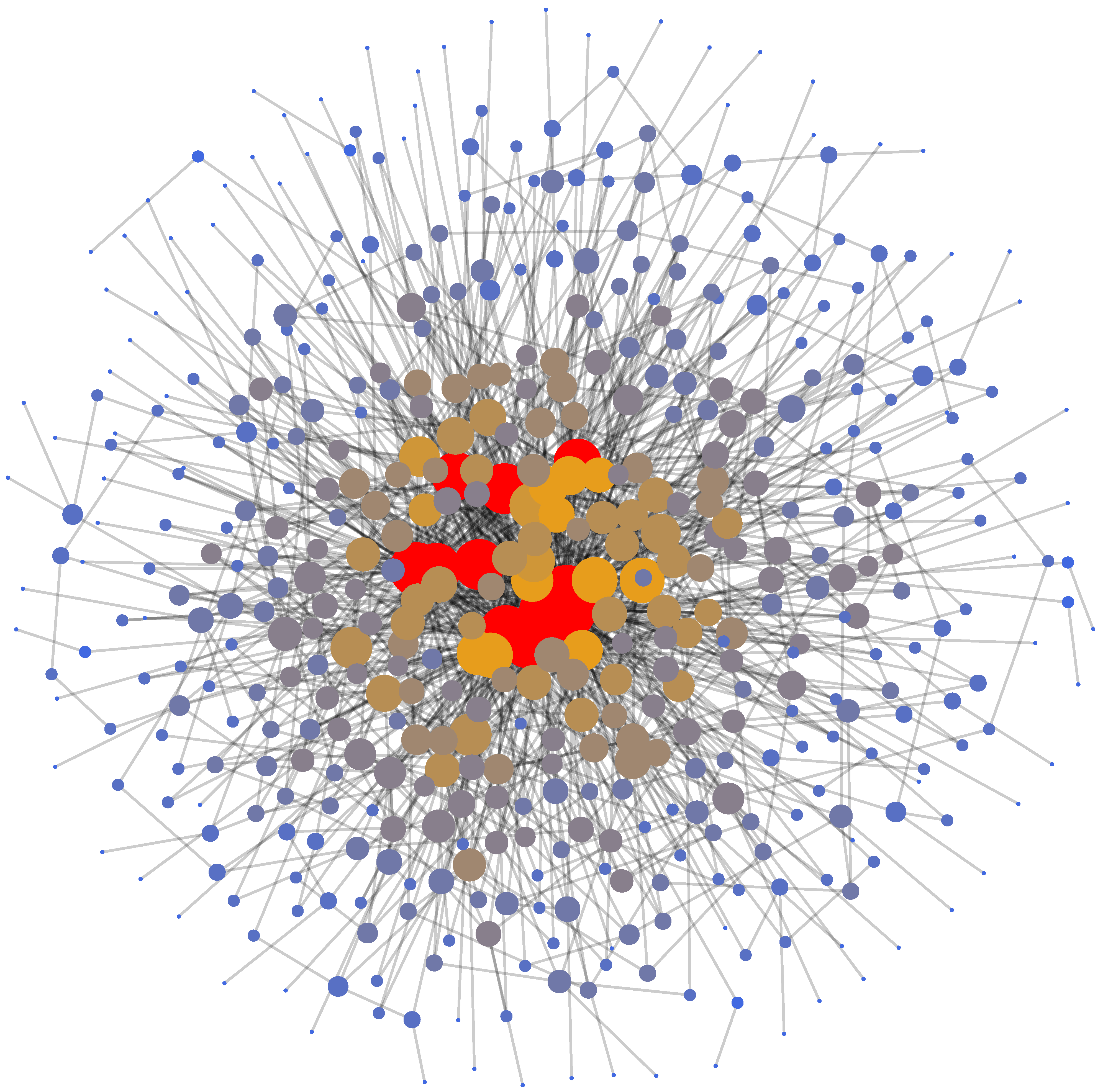
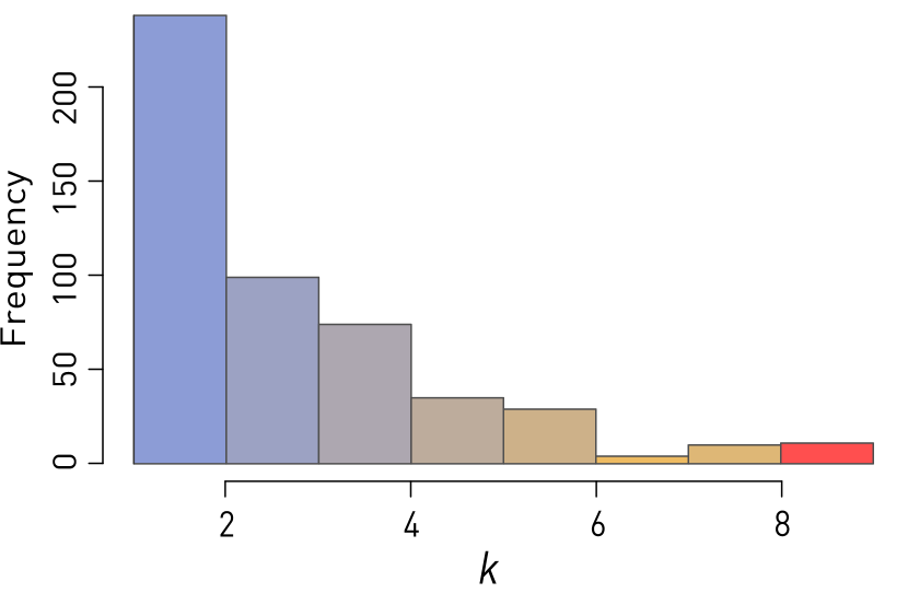
Their intra-layer topology shows a scale-free degree distribution and a core-periphery structure.
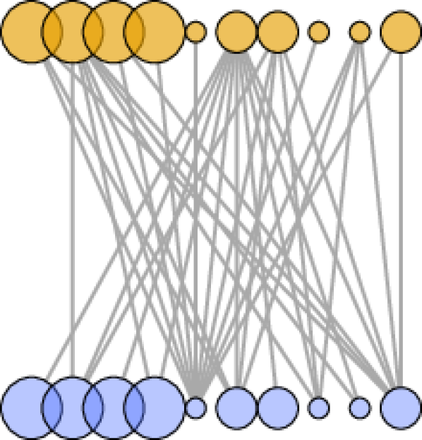
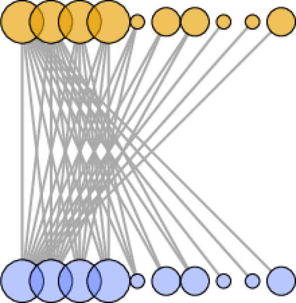
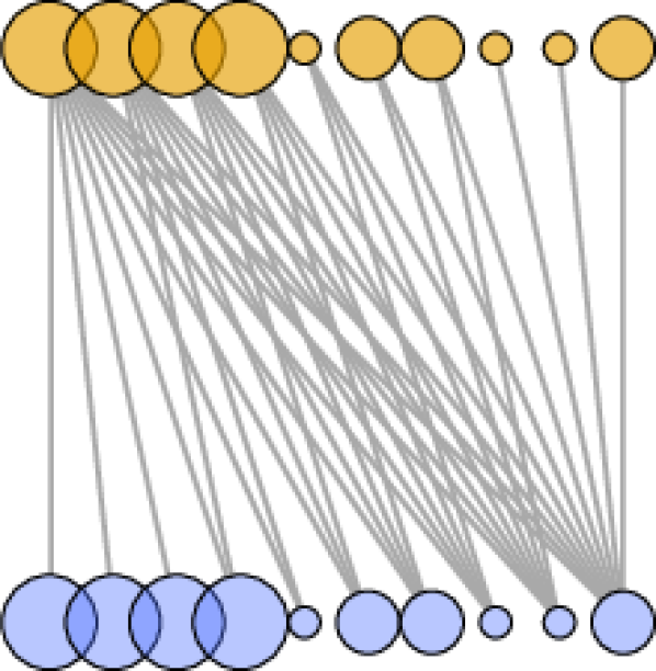
A nested structure describes the inter-layer topology, i.e., some nodes from , the generalists, have many links to nodes in , specialists only have a few.
This structure is verified by analyzing two empirical networks from ecology and economics.
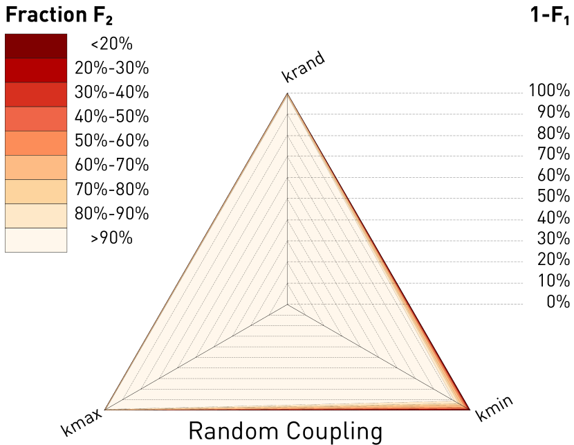
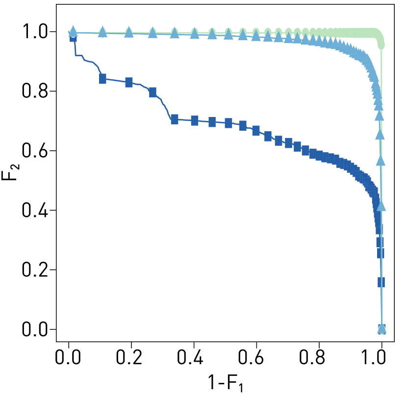
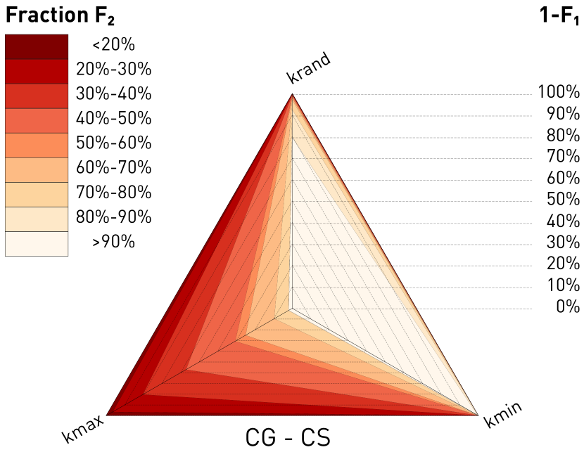
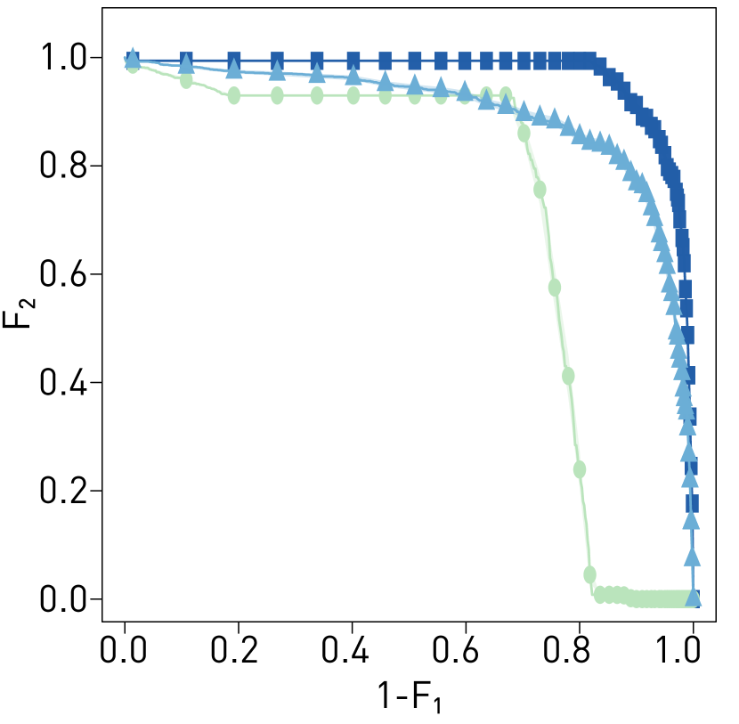
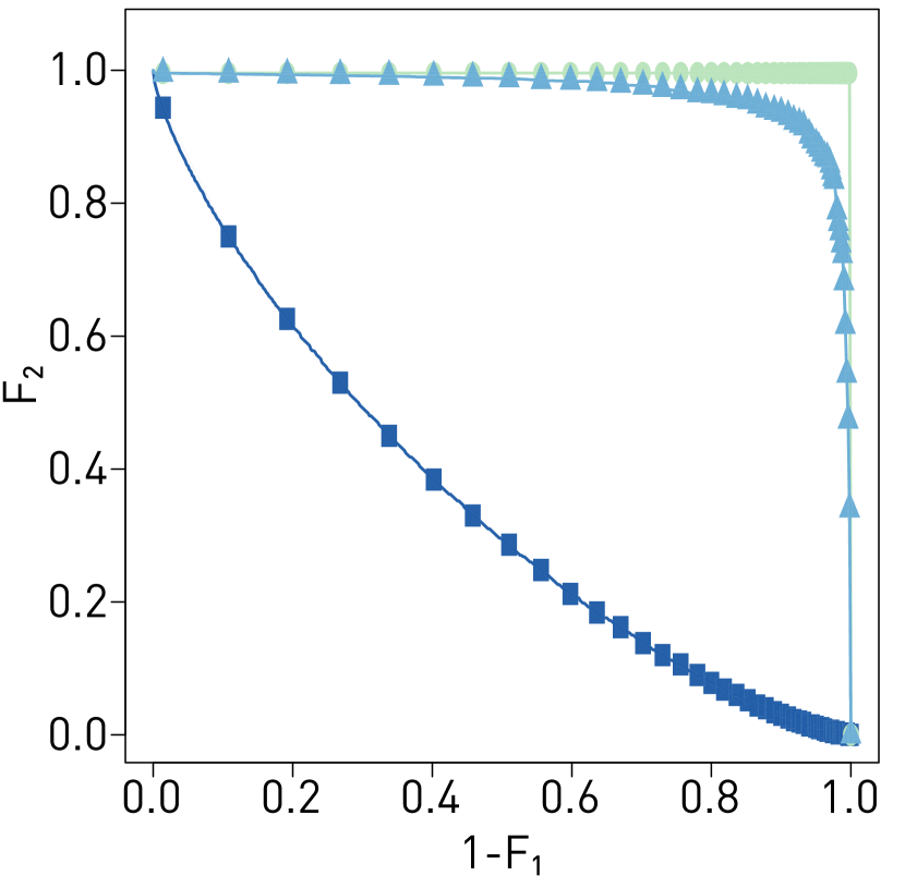
To probe the robustness of the multi-layer network, we remove nodes from with their inter- and intra-layer links and measure the impact on the size of the largest connected component, , in , which we take as a robustness measure.
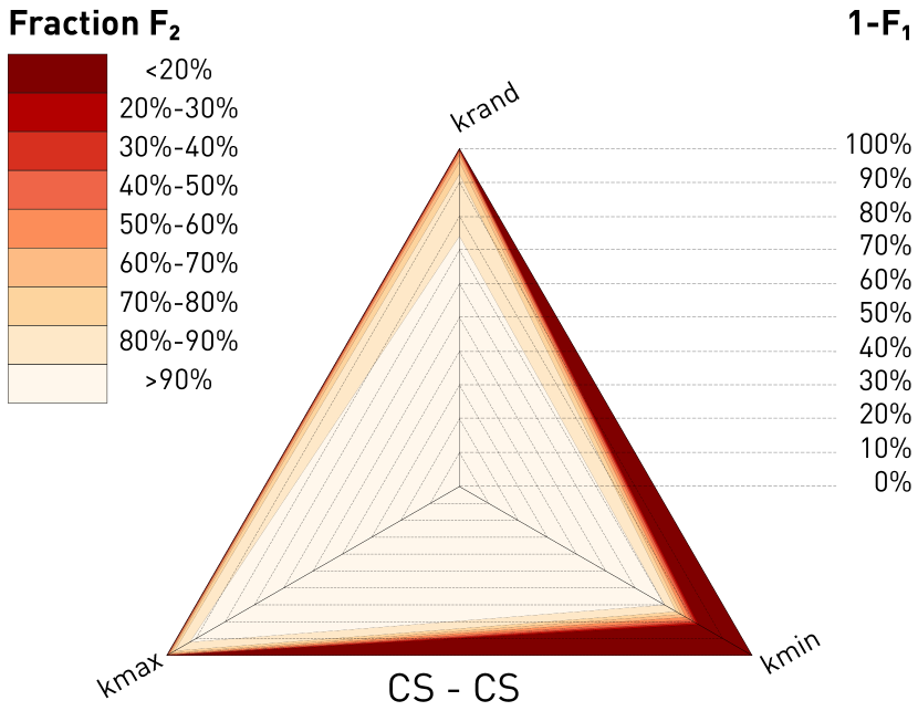
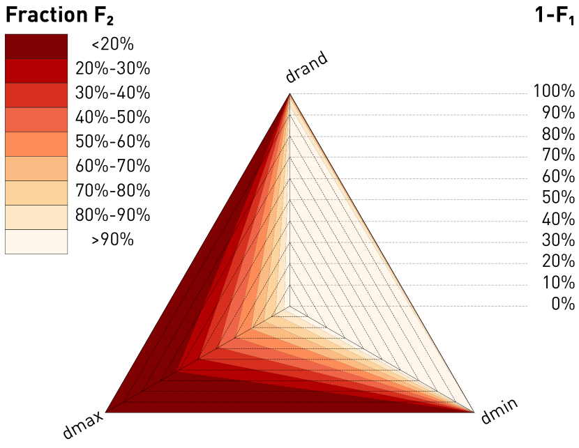
We test different attack scenarios by preferably removing peripheral or core nodes.
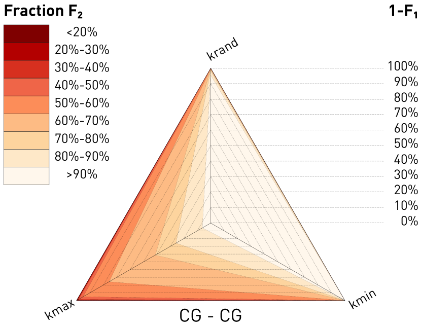
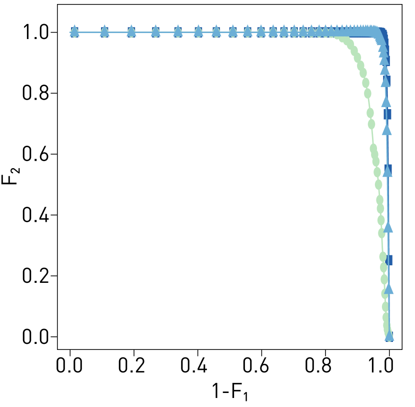
We also vary the intra-layer coupling between generalists and specialists, to study their impact on the robustness of the multi-layer network.
We find that some combinations of attack scenario and intra-layer coupling lead to very low robustness values, whereas others demonstrate high robustness of the multi-layer network because of the intra-layer links.
Our results shed new light on the robustness of bipartite networks, which consider only inter-layer, but no intra-layer links.
1 Introduction
2 Methods
2.1 A multi-layer network
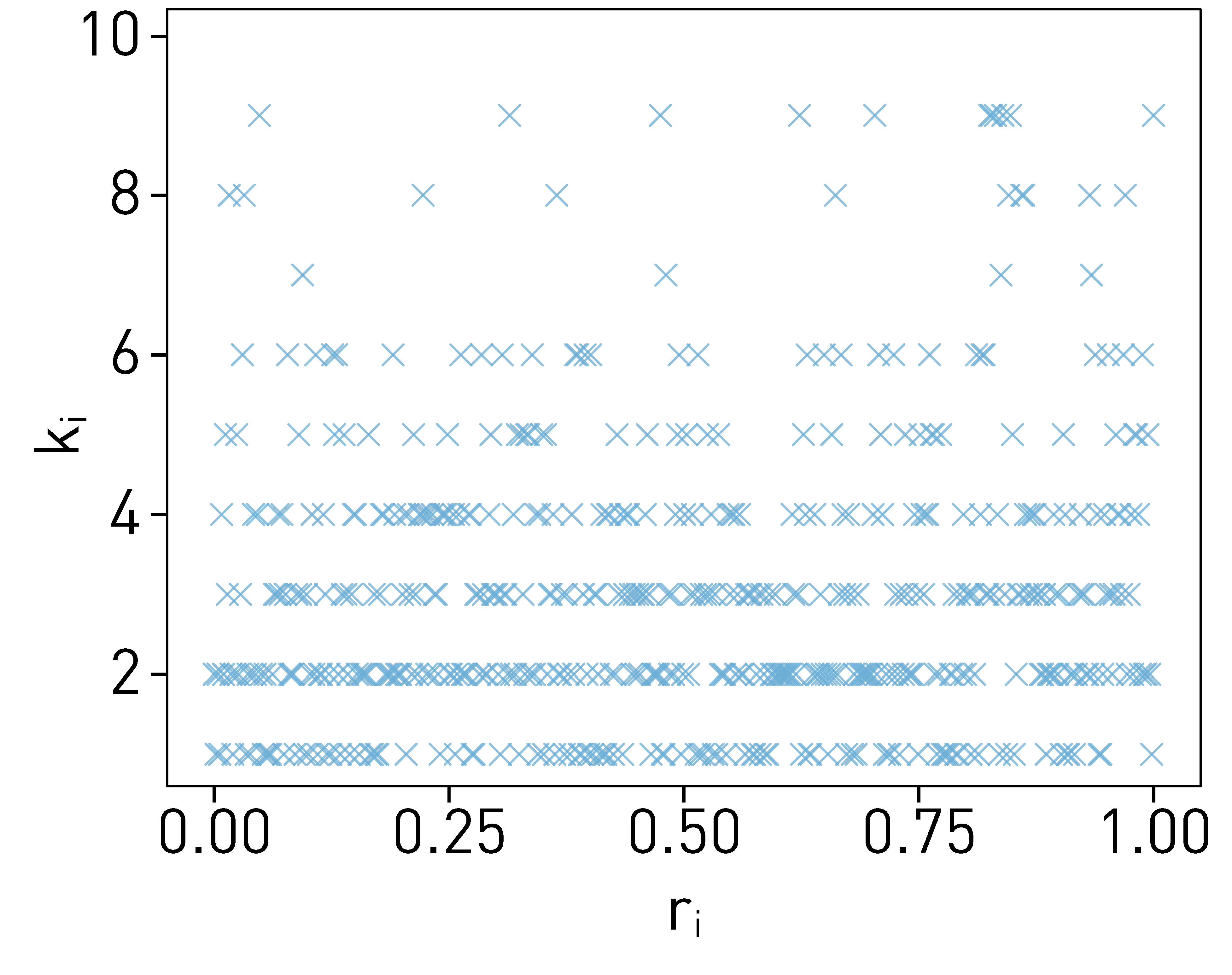
2.2 Intra-layer topology
Degree distribution.
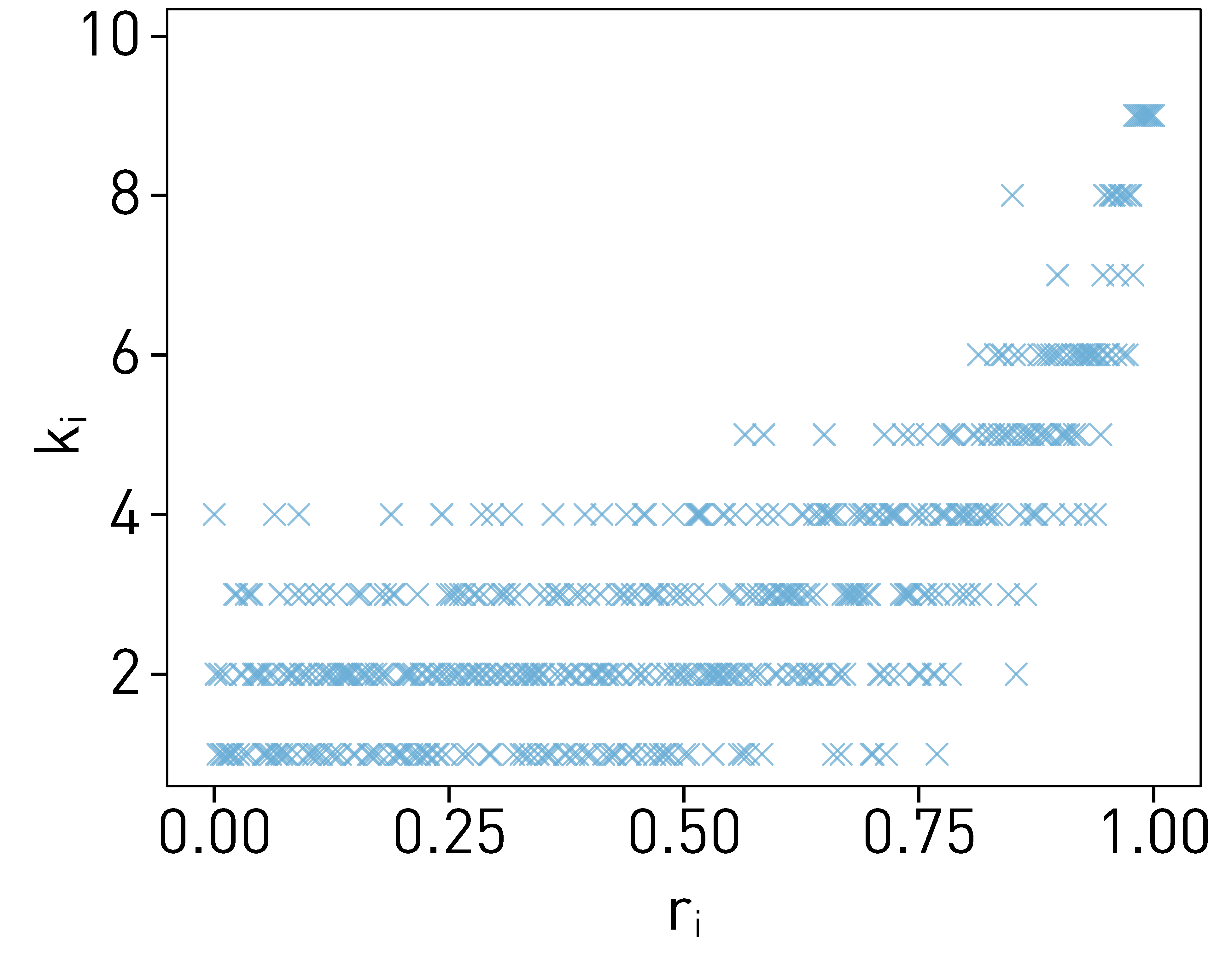
Coreness.
2.3 Inter-layer topology
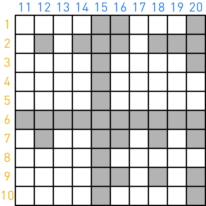
Bipartite networks.
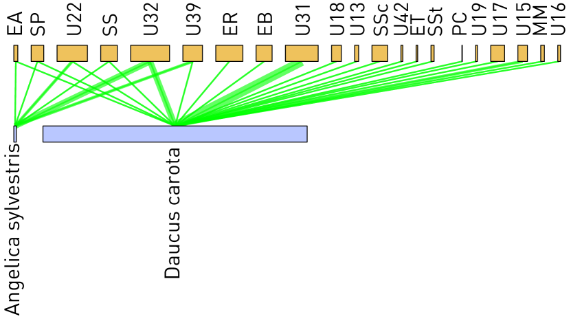
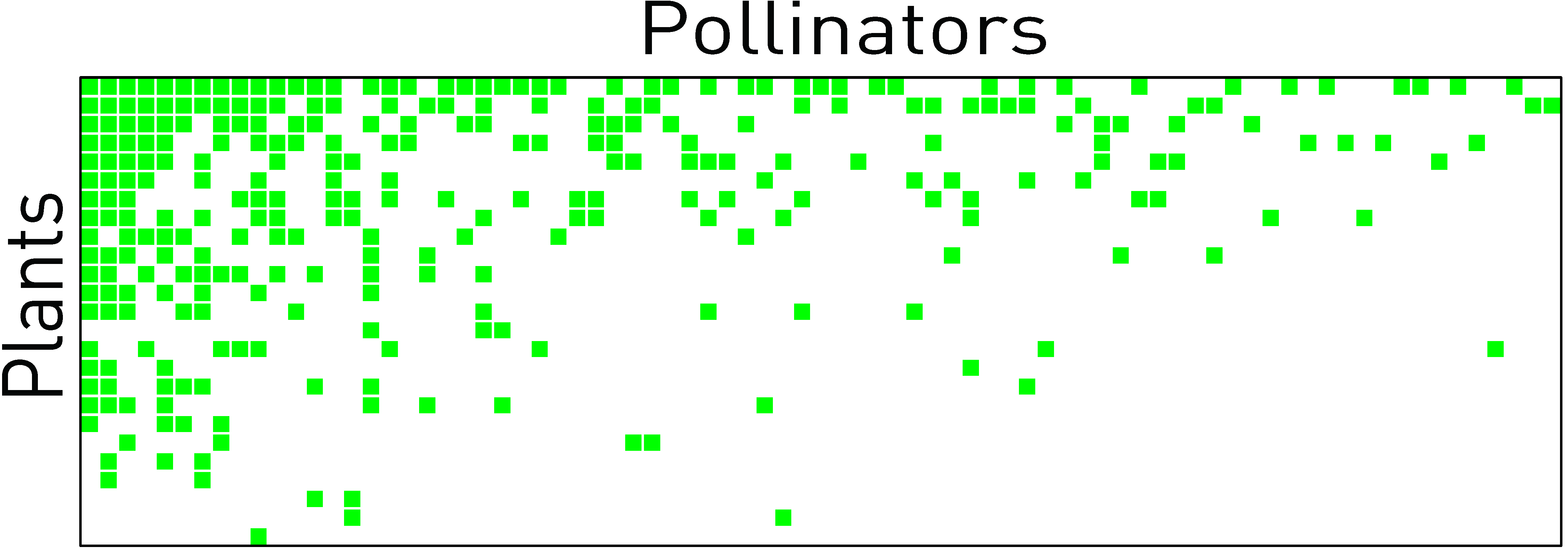
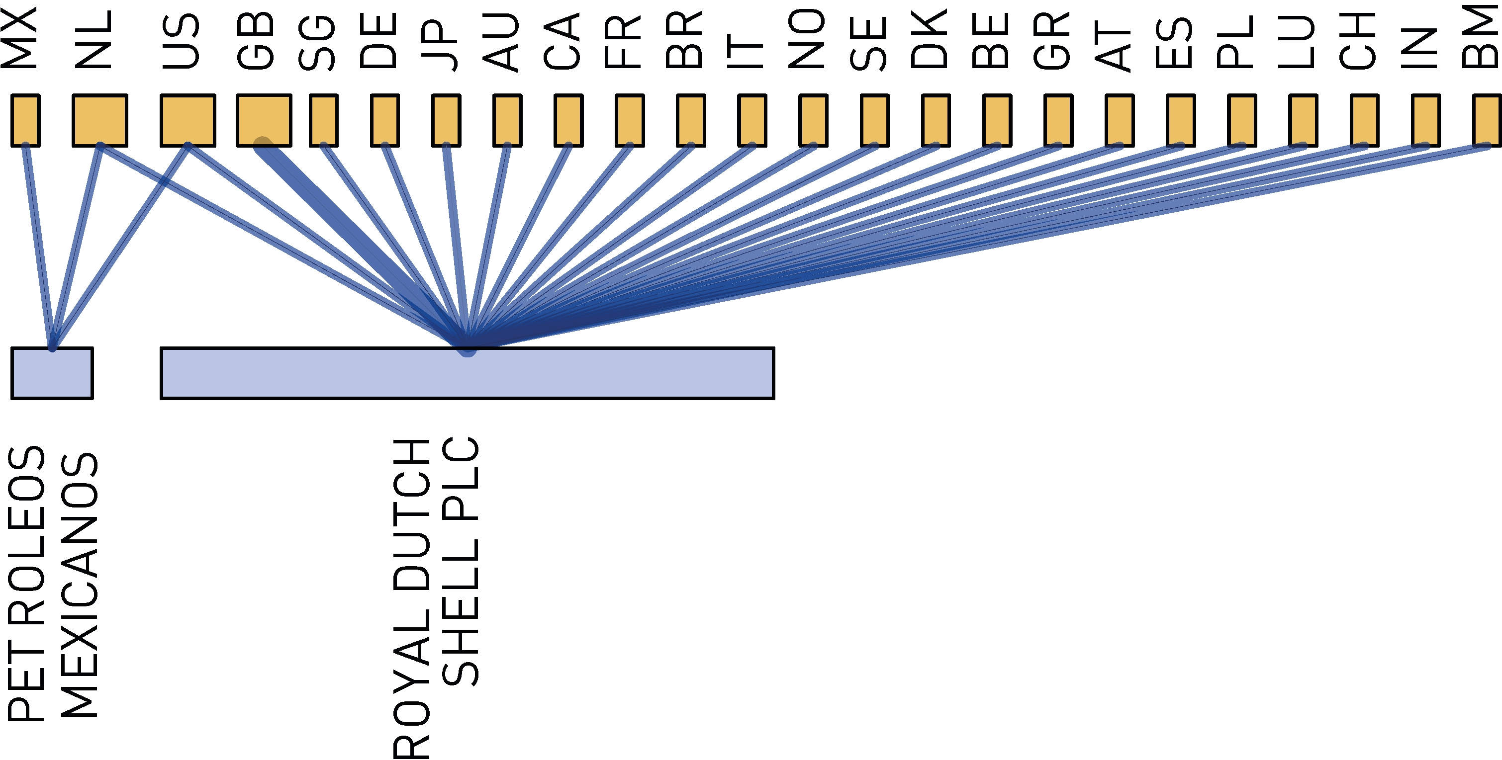
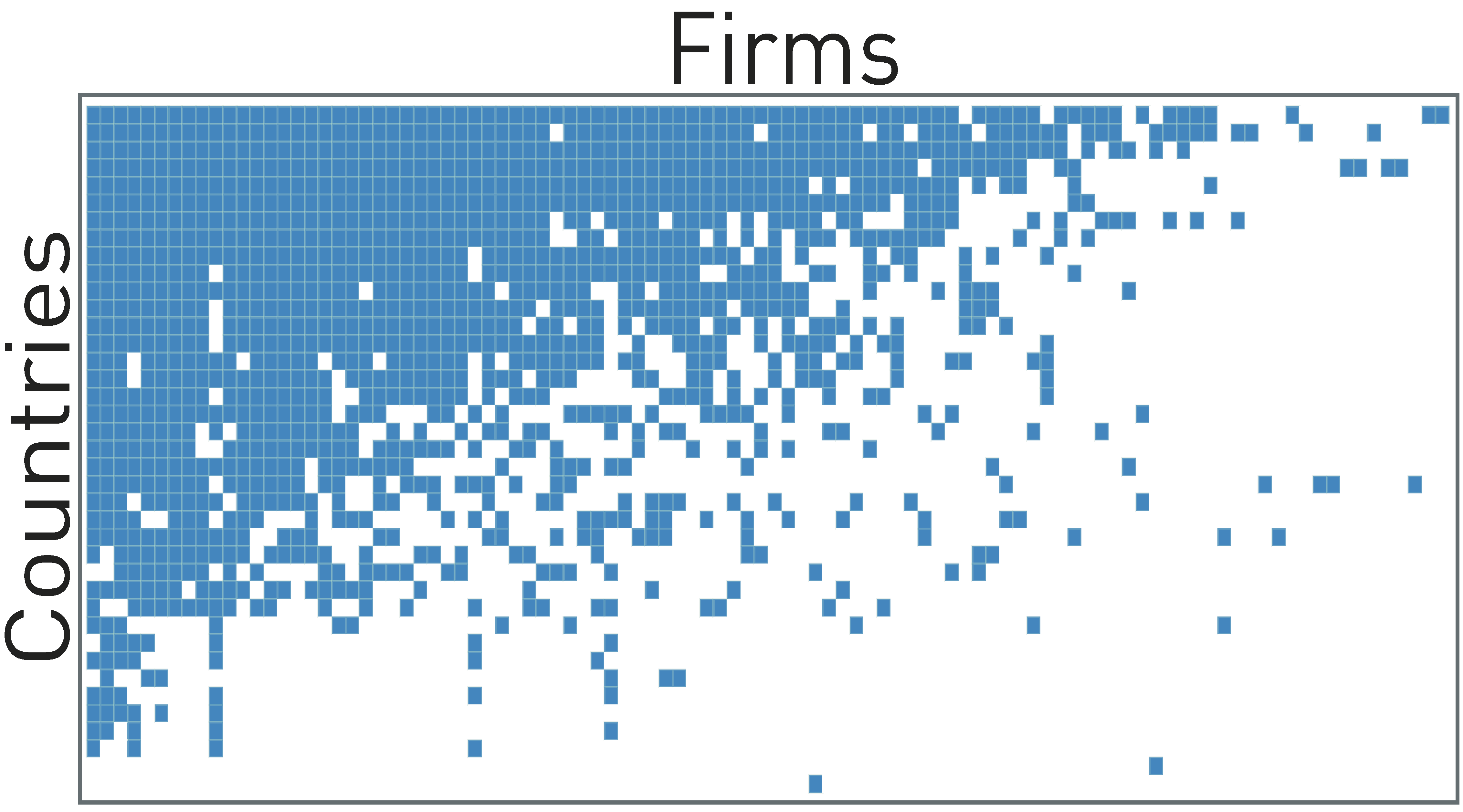
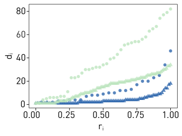
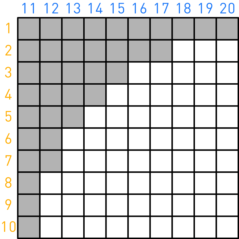
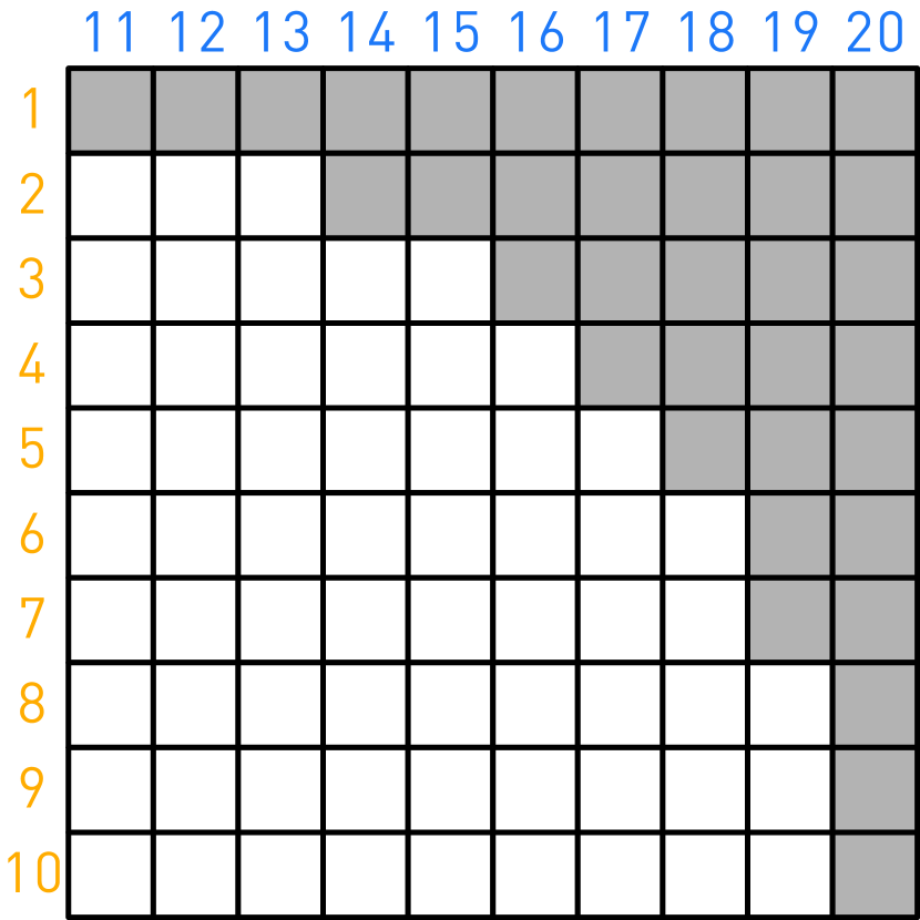
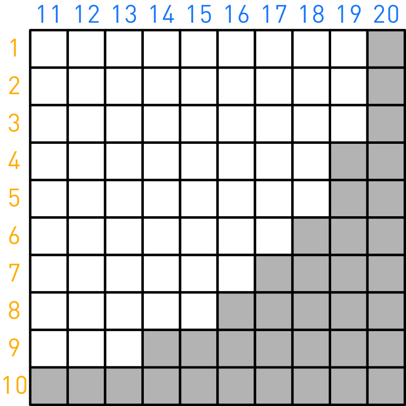
Nestedness.
Quantifying nestedness.
2.4 Scenarios to probe robustness
Attack scenarios.
Selection of nodes for removal.
Removal of nodes.
Influence of the inter-layer coupling.
3 Results
3.1 Robustness of the ecological sample network
3.2 Robustness of the full model