Probabilistic One-Dimensional Inversion of Frequency-Domain Electromagnetic Data Using a Kalman Ensemble Generator

Abstract

Frequency-domain electromagnetic (FDEM) data of the subsurface are determined by electrical conductivity and magnetic susceptibility. We apply a Kalman Ensemble generator (KEG) to one-dimensional probabilistic multi-layer inversion of FDEM data to derive conductivity and susceptibility simultaneously. The KEG provides an efficient alternative to an exhaustive Bayesian framework for FDEM inversion, including a measure for the uncertainty of the inversion result. Additionally, the method provides a measure for the depth below which the measurement is insensitive to the parameters of the subsurface. This so-called depth of investigation is derived from ensemble covariances. A synthetic and a field data example reveal how the KEG approach can be applied to FDEM data and how FDEM calibration data and prior beliefs can be combined in the inversion procedure. For the field data set, many inversions for one-dimensional subsurface models are performed at neighbouring measurement locations. Assuming identical prior models for these inversions, we save computational time by re-using the initial KEG ensemble across all measurement locations.

$\copyright$ 2019 IEEE. Personal use of this material is permitted. Permission from IEEE must be obtained for all other uses, in any current or future media, including reprinting/republishing this material for advertising or promotional purposes, creating new collective works, for resale or redistribution to servers or lists, or reuse of any copyrighted component of this work in other works.

1 Introduction

Exploring the subsurface electrical conductivity (EC) and magnetic susceptibility (MS) is interesting to geophysicists as anomalies in both quantities can often be associated with resources, geological structures, contamination or human activity. Frequency-domain electromagnetic (FDEM) measurements are determined by the EC and MS of the subsurface. In recent years, new applications of FDEM measurements have been explored and the design of FDEM has been tailored to facilitate survey practice. These developments have enabled surveying large areas efficiently (e.g., [1] and [2]), and surveying in highly conductive and/or magnetic environments (e.g., [3] and [4]). Inversions of such data sets may require large computational effort for two reasons: the size of the data set itself, and the non-linearity of the forward model exceeding the conditions of the low-induction number approximation [5] requiring non-linear inversion methods. To tackle these issues, we present an efficient probabilistic inversion method for FDEM data based on the Kalman ensemble generator (KEG, [6]). We use a non-linear forward model that applies a full solution of Maxwell’s equations.

The KEG presented here uses both the in-phase (IP) and out-of-phase (OP) component of the FDEM response to invert for subsurface EC and MS simultaneously. Earlier work on FDEM inversion, for example by [7], [8], [9], and [10], emphasizes the importance of using both components of the response to receive reliable inversion results in magnetic environments. In particular, Beard and Nyquist [7] describe how including the IP component can avoid systematic underestimation of EC when a significant IP shift is recorded.

The aforementioned publications apply classical, deterministic inversion approaches yielding a single model parameter realisation [11]. We propose a pragmatic approach to probabilistic FDEM inversion by applying the ensemble-based KEG. The KEG method can be seen as a trade-off between two extreme approaches to inverse problems: (1) using a deterministic inversion that quickly finds a single model satisfying the data, and (2) computing a large number of possible parameter models in search techniques aiming to be exhaustive (e.g., Markov-chain Monte-Carlo methods [12]).

Ensemble-based inversions have been proven to be efficient and robust [6], but at the same time comprehensive enough to characterize the uncertainty of the result. In the context of Kalman methods, uncertainty is characterized by standard deviations (STD) of model parameters, which are a measure for the parameter spread of the models that match the field measurements. The KEG method uses an equation equal to the update step of the Ensemble Kalman Filter [13], but it performs updates exclusively in the model parameters [6].

The novelty of our work lies in the application of the KEG to the inversion of FDEM data. We update prior EC and MS ensembles simultaneously, based on the measurements of the IP and OP component of the secondary electromagnetic field. Additionally, it is shown how correlations computed in the KEG can be used as a proxy for the measurement sensitivity. Using this sensitivity proxy, we determine a depth of negligible sensitivity, the so-called depth of investigation of a particular measurement setup. The KEG provides an interesting inversion method for geophysical data, especially when moving towards large and multi-dimensional forward models.

The application of the KEG is demonstrated for multi-configuration FDEM data: first, on synthetic data including vertical variation in both EC and MS, and second, on a field data set from an archaeological site in Dorset, United Kingdom. The field data was collected with a small-loop FDEM device consisting of one transmitter and several fixed receiver coils rigidly installed on a mobile sled system. This way, all data points in the field data set were acquired using an identical measurement setup. Our results show that the KEG can be used for simultaneous inversion of EC and MS. We show how the method delivers model uncertainties. Additionally, it is demonstrated that, if the same prior model is assumed for multiple data points, a single prior ensemble can be re-used in the inversions at these multiple data points.

2 Methodology

2.1 Forward model

A popular measurement setup for FDEM data are so-called loop-loop systems, which are characterized by the usage of one transmitter coil and one or multiple distinct receiver coils [14]. The transmitter coil is excited by an alternating current. It generates the primary electromagnetic field which propagates into the subsurface and induces alternating eddy currents in conducting material. These eddy currents generate a secondary magnetic field which is detected by one or multiple receiver coils. FDEM data are often expressed in terms of the in-phase (IP) and 90 degrees out-of-phase (OP) components with respect to the primary electromagnetic field. For low-frequency applications, applying a quasi-static approximation, these components are mainly influenced by electrical conductivity (EC) and magnetic susceptibility (MS), whereas dielectric permittivity is negligible.

We compute the forward model response according to Maxwell’s equations for a one-dimensional, horizontally layered half-space. This forward model accounts for vertical variation of EC and MS (Figure 1). As input for the computation of the FDEM measurement response, we choose a certain coil configuration (geometry, frequency of the primary field and transmitter moment) and subsurface realization (discretization and electromagnetic properties), in which the deepest layer is assumed to extend to infinite depth [15].

For the horizontal co-planar (HCP) coil configurations, the magnetic field $\mathbf{H}_{ZZ}$ at the receiver coil is expressed by the following equation [16]:

$$\mathbf{H}_{ZZ}=\frac{m}{4\pi}\int_{0}^{\infty}\left[\textrm{e}^{u_{0}(z+h^{tx})}+r_{TE}\textrm{e}^{u_{0}(z-h^{tx})}\right]\frac{\lambda^{3}}{u_{0}}\mathbf{B}_{0}(\lambda\mathbf{r})\textrm{d}\lambda$$ (1)

where $m$ is the transmitter moment, $h^{tx}$ is the height of the transmitter coil above ground, $\mathbf{r}$ is the separation of transmitter and receiver coil, $\lambda=(k^{2}_{x}+k^{2}_{y})^{1/2}$ is the horizontal wave number; whereby $u_{i}=(\lambda^{2}-k_{i}^{2})^{1/2}$, in which $k_{i}=(\omega^{2}\mu_{i}\epsilon_{i}-j\omega\mu_{i}\sigma_{i})^{1/2}$ is the wave number of the ith layer, with the angular frequency $\omega$; $\sigma_{i}$ the conductivity, $\mu_{i}$ the magnetic permeability, and $\epsilon_{i}$ the dielectric permittivity of the layer $i$; $j$ is the imaginary unit $j^{2}=-1$; $\mathbf{B}_{0}$ is the Bessel function of zeroth order; $r_{TE}$ is the reflection coefficient calculated for a layered medium by the recursive formula given by Ward and Hohmann [16]. We perform the Hankel $\mathbf{J}_{0}$ and $\mathbf{J}_{1}$ transforms using the digital linear filter as described by Guptasarma and Singh [17]. Formulas for the magnetic field of other dipole orientations analogous to equation 1 are provided by Ward and Hohmann [16].

FDEM data $\mathbf{d}(\omega)$ are presented in parts-per-million (ppm) of the primary field [12]:

$$\mathbf{d}(\omega)=\frac{\mathbf{H}(\omega)-\mathbf{H}^{0}(\omega)}{\mathbf{H}^{0}(\omega)}\cdot 10^{6}$$ (2)

where $\mathbf{H}$ is the total magnetic field (e.g., equation 1) and $\mathbf{H}^{0}$ is the magnetic field of free space.

2.2 Bayesian parameter estimation in inverse problems

In the next sections we will motivate our usage of the Kalman ensemble generator (KEG) as an approximate solution of the Bayesian parameter estimation problem. The Bayesian parameter estimation problem [18] consists of finding the so-called posterior probability distribution $\rho(\mathbf{m}\mid\mathbf{d})$. Here, $\mathbf{m}\in\mathbb{R}^{n_{m}}$ is a vector containing random variables for each of the $n_{m}$ parameters to be estimated. In this study, $\mathbf{m}$ includes subsurface EC and MS for all discretized subsurface layers. The vector $\mathbf{d}\in\mathbb{R}^{n_{d}}$ contains the $n_{d}$ observed random variables, on which the estimation is conditioned. The forward model from the previous section will be called $g$ from now on. The forward model $g$ allows to calculate a set of simulated measurement data $\mathbf{d}_{sim}=g(\mathbf{m})$. Exact knowledge of the true physical parameters and a perfect forward model would yield $\mathbf{d}_{obs}=\mathbf{d}_{sim}$, where $\mathbf{d}_{obs}$ are the means of unbiased measurements. The posterior distribution $\rho(\mathbf{m}\mid\mathbf{d})$ is given by Bayes’ theorem

$$\rho(\mathbf{m}\mid\mathbf{d})=\kappa\cdot\rho_{M}(\mathbf{m})\rho_{D}(\mathbf{d}\mid\mathbf{m}),$$ (3)

with a normalization constant $\kappa$ [18]. In the inversion, we use $\rho_{D}(\mathbf{d}\mid\mathbf{m})$, the likelihood of a certain set of measurements $\mathbf{d}$ given a set of parameters $\mathbf{m}$. Computing this likelihood, the simulated measurements $\mathbf{d}_{sim}$ are compared to the actual measurements $\mathbf{d}_{obs}+\epsilon$, which are assumed to be unbiased with random measurement error $\epsilon$. The prior information on the parameters is collected in the probability density function (PDF) $\rho_{M}(\mathbf{m})$. Below, incorporation of prior information will be further discussed.

2.3 Least-squares

Inverse problems are often solved applying variations of the least-squares approach. Likewise, the KEG can be motivated starting from a probabilistic least-squares approach. Readers familiar with the latter might want to skip the following section.

A derivation of least-squares as the solution of the Bayesian parameter estimation problem for Gaussian probability distributions and independent measurements is given by Tarantola [19], Chapter 3. Gaussian prior information can be given as

$$\rho_{M}(\mathbf{m})=\textrm{const}\cdot\textrm{exp}(-\frac{1}{2}(\mathbf{m}-\mathbf{m}_{prior})^{T}\mathbf{C}^{-1}_{M}(\mathbf{m}-\mathbf{m}_{prior})),$$ (4)

stating that the model $\mathbf{m}$ is a sample of the Gaussian prior with mean $\mathbf{m}_{prior}$ and covariance matrix $\mathbf{C}_{M}$. The Gaussian PDF for the measurement variables $\mathbf{d}$ is of the same form as equation 4 with mean $\mathbf{d}_{obs}$ and the corresponding covariance matrix of random observation errors $\mathbf{C}_{D}$. For measurements with Gaussian noise and parameters $\mathbf{m}$ with Gaussian PDFs, a linear forward model $g$ will lead to a Gaussian posterior PDF. The further the relation $\mathbf{d}=g(\mathbf{m})$ deviates from being linear, the further the posterior PDF deviates from being Gaussian.

For nonlinear problems, Tarantola [19] linearizes the forward function around $\mathbf{m}_{prior}$ and approximates:

$$g(\mathbf{m})\simeq g(\mathbf{m}_{prior})+Dg(\mathbf{m}-\mathbf{m}_{prior}),$$ (5)

where $Dg$ is the Jacobian matrix of $g$ at $\mathbf{m}_{prior}$. The Gaussian posterior is defined by its posterior mean $\mathbf{\widetilde{m}}$ and covariance $\mathbf{\widetilde{C}}_{M}$:

$$\mathbf{\widetilde{m}}\simeq\mathbf{m}_{prior}+\mathbf{C}_{M}Dg^{T}(Dg\mathbf{C}_{M}Dg^{T}+\mathbf{C}_{D})^{-1}\cdot(\mathbf{d}_{obs}-g(\mathbf{m}_{prior}))$$ (6)

and

$$\mathbf{\widetilde{C}}_{M}\simeq(Dg^{T}\mathbf{C}_{D}^{-1}Dg+\mathbf{C}_{M}^{-1})^{-1}.$$ (7)

As stated by Tarantola [19], equation 6 and 7 are equivalent to the sequentially applied update equations of the Kalman Filter [20] as derived for linear stochastic systems.

2.4 Kalman ensemble generator

The Kalman ensemble generator is a parameter estimation algorithm based on the update equation of the Ensemble Kalman Filter (EnKF, [13]). The EnKF is a widely used data assimilation method. It was introduced as a computationally more efficient alternative to the classical Kalman Filter [20], which is a sequential application of least squares. The EnKF uses an ensemble of states and parameters which is updated using the so-called Kalman formula (equation 8 as implemented).

The efficiency of the EnKF, and thus KEG, comes from the approximation of all Gaussian PDFs by an ensemble. An ensemble consists of a number of random samples drawn from a PDF, the so-called ensemble members. In this sense, the EnKF is a Monte Carlo implementation of the Bayesian update problem [21]. Covariance matrices are replaced by sample covariances and the approach can be understood as an ensemble-based approach to Kalman filtering.

The EnKF has been used in state estimation (e.g., [21]), parameter estimation, and mixtures of both (e.g., [22]). If the Gaussian assumption for all involved PDFs is applicable, the EnKF can be used for parameter and state estimations in nonlinear systems [23]. The stationary parameter estimation approach has been described by Nowak [6] and called the Kalman ensemble generator (KEG) to differentiate it from the classical Ensemble Kalman approaches.

The prior ensemble of the KEG is a collection of randomly drawn samples from the prior PDF. If the prior PDF is Gaussian as in equation 4, Gaussian random samples can be determined by a prior mean and the covariance matrix (see next section and Figure 1). More general prior PDFs are possible, but it has to be kept in mind that the derivation of the equations for least-squares parameter estimation makes use of the Gaussianity of the PDFs. The total number of samples is called $n_{ens}$. All samples are collected in the ensemble matrix $\mathbf{A}\in\mathbb{R}^{n_{m}\times n_{ens}}$.

Given $m$ discrete subsurface layers, the number of estimated parameters for EC and MS is $n_{m}=2m$. These subsurface parameters are treated as random variables. The prior ensembles are updated using the equation [13]:

$$\mathbf{A}^{Update}=\mathbf{A}+\mathbf{A^{\prime}G^{\prime}}^{T}(\mathbf{G^{\prime}G^{\prime}}^{T}+\mathbf{EE}^{T})^{-1}(\mathbf{D-G}),$$ (8)

where $\mathbf{A}^{Update}\in\mathbb{R}^{2m\times n_{ens}}$ is the posterior ensemble matrix, the update of the prior ensemble matrix $\mathbf{A}\in\mathbb{R}^{2m\times n_{ens}}$. $\mathbf{A}^{\prime}\in\mathbb{R}^{2m\times n_{ens}}$ is the ensemble matrix $\mathbf{A}$ after substracting the mean value of each column from this column. $\mathbf{D}\in\mathbb{R}^{n_{coils}\times n_{ens}}$ is the data matrix containing an ensemble of FDEM measurements. The ensembles in $\mathbf{D}$ are generated from Gaussian PDFs with the IP and OP measurement as mean and measurement noise as standard deviation. $\mathbf{E}\in\mathbb{R}^{n_{coils}\times n_{ens}}$ is the data matrix $\mathbf{D}$ after substracting the mean value of each column from this column. $\mathbf{E}$ can be derived from the covariance matrix of random observation errors by Cholesky decomposition $\mathbf{C}_{D}=\mathbf{E}\cdot\mathbf{E}^{T}$. In the response matrix $\mathbf{G}=g(\mathbf{A})\in\mathbb{R}^{n_{coils}\times n_{ens}}$, we collect the responses of the samples in $\mathbf{A}$. In contrast to $Dg$ from least-squares, no linearization around $\mathbf{m}_{prior}$ is used in the computation of $\mathbf{G}$. $\mathbf{G^{\prime}}$ is $\mathbf{G}$ after substracting the mean value of each column from this column.

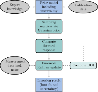
Figure 2: Flow chart of the KEG inversion: Starting from the prior estimation of the model parameters, a prior ensemble (Fig. 1) is generated by sampling the EC and MS multivariate Gaussian prior. Correlation of prior and corresponding forward response ensemble can be used to compute the depth of investigation (DOI). The forward responses to the prior ensemble and the measurement ensemble are used to create an Ensemble Kalman update of the prior model. This update gives the posterior model: the inversion result.

The mean values of the samples in $\mathbf{A}^{Update}$ are considered as the best-fit-solution to the measurement data, with their standard deviation representing the uncertainty of this fit. For Gaussian PDFs and a linear forward model, the best fit solution is equivalent to the Maximum A Posteriori estimate (MAP, [11]). In contrast to classical inversion and similar to other Bayesian methods, the KEG allows to derive an inversion result without introducing further regularization to the processing. This is possible because a regularization is implicitly introduced by the determination of parameters through their PDFs. For Gaussian PDFs, this implicit regularization can be shown to correspond to least-squares with Tikhonov regularization [11]. An overview of the inversion approach is shown in Figure 2.

In contrast to the least-squares approach from the previous section, where mean equation 6 and covariance equation 7 solve the inversion, for the KEG, one matrix update equation is used to derive posterior mean and covariance (equation 8). Equation 8 can be understood as $n_{ens}$ least-squares computations. For Gaussian PDFs, a linear forward model, and infinitely large ensembles, the KEG is equivalent to the least-squares approach. The KEG has two advantages over equation 6 and 7. First, all covariances are computed from the ensembles, which is fast. Second, the KEG does not linearize $g$ around $\mathbf{m}_{prior}$. Even though a linearization is still implicit in the least-squares-like update step, calculating the full forward model reduces the error caused by non-linearities in the misfit $(\mathbf{D}-\mathbf{G})$ and the calculation of covariances using $\mathbf{G}^{\prime}$. Assuming not too strong non-linearities around the chosen $\mathbf{m}_{prior}$, we derive the uncertainty of the result at much reduced cost as compared to the commonly applied MCMC methods (see following paragraph).

Comparison to MCMC

We compare the KEG approach to well-established Markov chain-Monte Carlo (MCMC) methods (e.g., [19] and [11]). An advantage of MCMC methods is that they can handle general non-linear inverse problems and converge to the exact solution of the parameter estimation problem in the limit of an infinite number of samples. Additionally, MCMC methods can be used for non-Gaussian PDFs. A drawback of MCMC methods is their large computational expense. They require an exhaustive search of the model space typically applying a Metropolis- or Gibbs-sampler. The results of the sampler form a Markov chain in which consecutive samples are correlated. This process has a lower efficiency than the KEG for three reasons: (1) the MCMC forward model runs cannot be parallelized, (2) the acceptance rate (for the Metropolis-sampler) is ideally between 30 and 50 $\%$ [19], and (3) to obtain uncorrelated samples only every $n$-th accepted sample can be used for the posterior distribution [24]. To highlight the importance of reducing the number of forward model runs, we take a look at the application of the KEG shown in section "Synthetic data set". There, the computation of the forward models requires approximately 97 $\%$ of the overall computing time. For larger forward models, minimizing the number of forward model runs could become crucial for the feasibility of probabilistic inversions. The KEG provides a computationally feasible alternative. As a trade-off, it is only a first-order approximation to the parameter estimation problem, meaning that only Gaussian probabilities can be modeled. However, the convergence to this first-order solution is so fast that the KEG might deliver smaller overall errors than comparable exact methods like MCMC approaches, especially for small CPU budgets.

2.5 Prior model

The selection of a prior model incorporates prior knowledge into the parameter estimation. This selection is important since the prior restricts the search space of parameter models. This is especially true for the KEG since the KEG is restricted to Gaussian parameter models. An underestimation of prior uncertainty could lead to best fits that lie far from the true parameter values, thus rendering the standard deviation (STD) meaningless. As for general probabilistic inversions, the results of the KEG have to be analyzed with these subtleties in mind.

In later chapters, we use vertically layered, one-dimensional model discretizations for the computations of the FDEM model. In this case, prior models for EC and MS are defined for each discretization layer. The prior should in principle be independent of the measured FDEM data. For each discretization layer, we use Gaussian prior guesses for EC and MS consisting of a mean and a STD for log-transformed EC or MS (Figure 1). The logarithm enforces positive values for EC and MS estimations, diamagnetic effects are neglected. The mean of the prior ensemble serves as expected value, the STD can be normalized by the mean to yield the coefficient of variation of log-transformed EC or MS. If model parameters are expected to be correlated, a multi-Gaussian prior can be defined through a mean vector and a covariance matrix.

The number of discretization layers is fixed throughout the inversion procedure and needs to be determined based on a trade-off between the computational cost, bias and the vertical model variability. A coarse discretization reduces the computational expense needed. In contrast, choosing a relatively finer discretization has two main advantages: (1) when the number of discrete layers is much larger than the number of expected subsurface layers, the influence of the discrete layer boundaries on the inversion result is reduced, and (2) a large number of inversion parameters entails only weak regularization and therefore reduces bias on the inversion result.

The prior is defined as a multivariate Gaussian distribution $N(\vec{\mu},\Sigma)$ [25]: collecting the expected values for the random parameters EC $\sigma$ and MS $\chi$ in the mean vector $\vec{\mu}$, and the corresponding variances and covariances in the covariance matrix $\Sigma$ [26].

Prior model parameter correlations are represented by off-diagonal covariances $\Sigma$ [27]:

$$\bm{\Sigma}(2m\times 2m)=$$

$$\begin{pmatrix}\mathrm{Var}(\sigma_{1})&\mathrm{Cov}(\sigma_{1},\sigma_{2})&\dotsb&\mathrm{Cov}(\sigma_{1},\chi_{2m})\\ \mathrm{Cov}(\sigma_{2},\sigma_{1})&\mathrm{Var}(\sigma_{2})&\mathrm{Cov}(\sigma_{2},\sigma_{3})&\\ \vdots&\ddots&\ddots&\vdots\\ \mathrm{Cov}(\chi_{2m},\sigma_{1})&\dotsb&\mathrm{Cov}(\chi_{2m},\chi_{2m-1})&\mathrm{Var}(\chi_{2m})\\ \end{pmatrix}.$$ (9)

In general, correlation is part of the prior model and should be chosen in accordance with the available a priori knowledge. For the examples in this manuscript, we express correlation in terms of a correlation function introduced by Gaspari and Cohn (section 4.3 in [28]) that approximates a Gaussian-shaped decrease of correlation in the covariance matrix. This way, we compute our prior covariances using the a priori defined STDs and a correlation length for the model parameters. In general, much more complicated correlation functions could be introduced, but for the few information that are usually available about the subsurface, STDs and a correlation length are a sufficiently complex representation.

For the KEG, an ensemble matrix $\mathbf{A}$ is created by collecting random samples from the multivariate Gaussian distribution (Fig. 1). This ensemble matrix contains an ensemble of prior model realizations, which are used as input for the forward model. A large ensemble size $n_{ens}$ is desirable since small ensembles can introduce bias to the processing steps of the KEG.

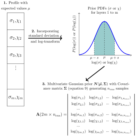
Figure 1: Creating the prior ensembles for ensemble matrix $\mathbf{A}$: Expected EC $\sigma$ and MS $\chi$ values are initialized for a profile with $m$ layers. Together with the standard deviation $s$ of fluctuations around these expectations, a multivariate Gaussian distribution is defined. Input ensembles are created through selecting $n_{ens}$ samples from this distribution.

In this study, we restrict our prior models to have spatially uniform mean and STD. This facilitates an evaluation of the KEG approach since the influence of the prior is minimized. In general, more sophisticated prior modeling, for example using geostatistical approaches, may improve inversion results (e.g., [29] and [26]).

2.6 Sensitivity and depth of investigation

Using the KEG, the measurement sensitivity can be expressed in terms of the correlation between the prior ensemble of EC or MS of a certain layer and the corresponding forward response. The depth of investigation (DOI) is usually defined as the depth from which surface data are insensitive to the investigated physical property of the subsurface [30]. Thus, if variation in prior realizations below a certain depth has no influence on the forward response the correlation should be zero. This is never exactly the case due to sampling uncertainty. But once the correlations are smaller than a certain threshold, it can be assumed from the correlation data that the depth of investigation is reached. The choice of the absolute threshold value is as arbitrary as for other DOI estimation methods [31]. In any case, the threshold correlation should be chosen larger than the present spurious correlation resulting from the undersampling bias. The covariance of the prior ensembles $\mathbf{A}$ and the forward response ensembles $\mathbf{G}$ are expressed by:

$$\textrm{{Cov}}(\mathbf{A,G}^{T})=\mathbf{A^{\prime}G^{\prime}}^{T}*\frac{1}{n_{ens}-1}$$ (10)

with the number of ensemble members $n_{ens}$. Normalizing equation 10 to the STDs of the respective parameters gives the correlation of these parameters for each layer assumed in the model. Since the matrix multiplication $\mathbf{A^{\prime}G^{\prime}}^{T}$ is part of the KEG (equation 8), it is available from the general algorithm without further computation.

The usage of the correlation as a sensitivity measure builds on the computation of different prior model realizations. In classical sensitivity estimation approaches, sensitivities are derived from finite-difference approximations [32]. This corresponds to a local slope analysis. For the KEG, not a local slope, but a global variance is analyzed and is here interpreted as a measurement sensitivity proxy.

3 Synthetic data set

We demonstrate the KEG inversion procedure on a one-dimensional synthetic subsurface model. The model includes a depth-dependency of both EC and MS realized in three layers (Fig. 4). The top layer is 50 cm thick, the intermediate layer is 1 m thick, the bottom layer extends to infinite depth. EC is set to 5 mS/m for the top layer, 20 mS/m for the intermediate layer, and 10 mS/m for the bottom layer. MS is set to 1$\cdot 10^{-5}$ for the top layer, 4$\cdot 10^{-5}$ for the intermediate layer and 1$\cdot 10^{-5}$ for the bottom layer.

Forward model responses are simulated at four assumed receiver coils, two coils in horizontal co-planar configuration (HCP) with 1 m and 2 m distance to the receiver, respectively, and two coils in perpendicular configuration (PRP) with a distance to transmitter of 1.1 m and 2.1 m, respectively. The coil centers are assumed 16 cm above the ground surface. The transmitter moment [16] of the transmitter coil is set to one. The operating frequency is set to 9000 Hz. These forward model parameters reflect the measurement set-up of the field data case discussed further below.

We choose a prior PDF consisting of Gaussian distributions. For each parameter (EC and MS), we assume spatial stationarity and specify constant mean and STD throughout the model domain. First, we simulate synthetic measurement samples of the logarithm-transformed synthetic true parameter values for intervals of 10 cm down to a depth of 5 m. These measurement samples are used as synthetic validation, thus playing the role of vertical in-situ measurements in a field data case. The mean of the prior PDF is chosen as the sample mean of the synthetic samples. The sample mean is 10.7 mS/m for EC, and 1.32$\cdot 10^{-5}$ for MS. For the same synthetic samples, the sample STD is calculated and used as the STD for the prior Gaussian PDF. After an inverse log-transform, the prior STD intervals range from 7.9 mS/m to 16.8 mS/m for EC and from 0.75$\cdot 10^{-5}$ and 2.8$\cdot 10^{-5}$ for MS (Fig. 4). For this example, there is no correlation introduced between the prior model parameters. This corresponds to the choice of a correlation length that is significantly smaller than the thickness of discretization layers. One motivation for this choice is the expectation of abrupt layer boundaries. Consequently, off-diagonal elements of the covariance matrix are zero (eq. 9). For the KEG, a prior ensemble of size 10,000 is created from the prior PDF.

First, we investigate the correlations between the prior parameter ensembles (EC and MS) and the forward responses (OP and IP). These correlations are shown in Figure 3a. The correlation between OP and MS fluctuates around zero for all four simulated receiver coils. The correlation between IP and EC is similarly small, but with values slightly larger than zero. Stronger correlation showing systematic variation is found for the correlations between OP and EC, and IP and MS. The general shape of these two correlation functions is in agreement with the respective differential sensitivity for the synthetic true model (Fig. 3b).

As significant correlation is present only between OP and EC, and IP and MS, we use these correlation functions for estimating the DOI of the simulated measurement setup. The respective DOIs are shown in Figure 3a. We set the DOI to the depth at which correlations for all coils fall below a threshold of 0.05. The DOIs are at 3.12 m for EC and 1.94 m for MS. This is in agreement with the shallower sensitivity for IP signals compared to OP signals as computed by perturbation of the synthetic true model ([32], Figure 3b).

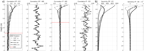
Figure 3: a) Correlation between the prior ensemble of EC and MS and the four simulated out-of-phase (OP) and in-phase (IP) electromagnetic signals. The depth of investigation (DOI) is marked where all correlations fall below the threshold 0.05; b) Sensitivities of the four simulated OP signals for EC (left) and the four simulated IP signals for MS (right) for the receiver coils. Sensitivities are derived from perturbations of the synthetic true model.

For the update step, the algorithm requires an additional ensemble of FDEM measurements. The STD for the synthetic measurement values was set to 0.01 ppm for both the OP and IP response.

The KEG update of the prior model, is shown in Figure 4 as best fit and corresponding posterior uncertainty. For both EC and MS, the best fit detects parameter value contrasts for the three layers present in the synthetic true model. Below the DOI, the best fit is a reproduction of the prior mean since equation 8 can be approximated by $\mathbf{A}^{Update}\approx\mathbf{A}$ for lowly correlated parameters.

The uncertainty of the best fit is shown as intervals of two standard deviations from the mean (Fig. 4). For all parameters, the synthetic true model is contained within these two standard deviations. The posterior uncertainty is smaller than the prior uncertainty in the top layer. Closer to the second layer, the best fit values as well as the uncertainty are larger. For the bottom layer, the synthetic true EC and MS are smaller than for the intermediate layer. Accordingly, the best fit renders lower values. The uncertainty is also decreasing from the center of the second layer downwards.

To evaluate the performance of the inversion approach, we calculate the RMSE between the best fit of the inversion result and the mean of the synthetic true for the whole model down to the respective DOI for EC and MS. The RMSEs are compared to the analogous RMSEs between prior model and synthetic true. Additionally, for the best fit vector and the prior mean vector, the corresponding IP and OP forward responses for the four coils are calculated. For these responses, the RMSE with the synthetic true response is computed. The RMSE values for IP and OP signals are finally summed up and shown in Table 1.

Table 1: Comparing the root mean square error (RMSE) of the synthetic ground truth with (1) mean vector of the prior ensembles and (2) best fit vector of the KEG inversion up to the respective DOI (Fig. 4), and the corresponding modelled measurement responses for in-phase (IP) and out-of-phase (OP) component for these respective vectors are compared to the synthetic-true measurement data by their respective RMSEs.

RMSE	EC profile	MS profile	OP-signal	IP-signal
Prior mean	5.5 mS/m	1.71$\cdot 10^{-5}$	42.4 ppm	4.2 ppm
Best fit	2.1 mS/m	0.9$\cdot 10^{-5}$	19.2 ppm	0.7 ppm

For EC the RMSE reduces from 5.5 mS/m for the prior model to 2.1 mS/m for the best fit. For MS the value reduces from 1.7$\cdot 10^{-5}$ to 0.9$\cdot 10^{-5}$. Decreased RMSEs for the best fit can also be observed for the OP and IP signal. For OP the value goes from 42.4 ppm to 19.2 ppm, for the IP signal the RMSE is reduced from 4.2 ppm to 0.7 ppm. The decreased RMSEs for the best fit are in accordance with the form of the best fit in Figure 4.

The computation time of the KEG update is 35.3 seconds. Of this total computation time, 34.3 seconds were consumed by the forward model runs. Thus, the repeated computation of forward models uses 97 $\%$ of the overall computation time, making the forward runs the most computationally expensive step in the inversion. When using a MCMC approach, we expect the number of forward model runs to be increased at least by a factor of three compared to the KEG. This illustrates how the KEG benefits computational efficiency.

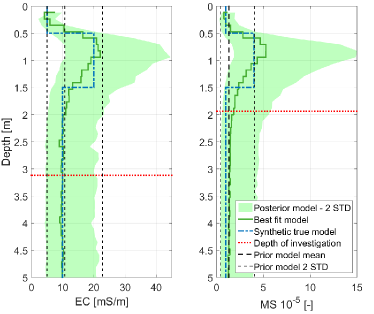
Figure 4: Statistics of the posterior PDFs for the KEG inversion of synthetic one-dimensional model: best fit (mean) and two standard deviations (STD) for EC (left) and MS (right), compared to the synthetic true. Additionally, the mean and two STDs of the prior PDFs and the depth of investigation are shown.

4 Field data set

An FDEM field data set was collected on a 1.3 ha area in Knowlton (Dorset, United Kingdom). The local subsurface is dominated by a thin rendzina soil cover (around 20 cm thick), developed in loessic sediments overlaying Cretaceous chalk bedrock. While the topsoil is strongly magnetic (MS in the order of 1$\cdot 10^{-3}$), the bedrock is diamagnetic rendering an overall background susceptibility of zero. Surveyed under dry conditions, the area has a low EC, varying around 7 mS/m, while the topsoil is slightly more conductive than the bedrock [33]. In the inversion, we aim to show the contrast in EC and MS between those layers. Additionally, the area is known for several henge structures from the Stone Age. These structures include man-made ditches which often cause magnetic anomalies in the near subsurface and thus may be detected by FDEM measurements [33].

For the FDEM measurement, a DUALEM-21S (Dualem, Canada), was used with simultaneous geo-referencing of the data points using a GPS device. The FDEM instrument configurations are identical to the one described in the section on the synthetic data set, i.e. two horizontal co-planar (HCP) and two perpendicular (PRP) coil set-ups.

FDEM data were collected along parallel lines in southwest-northeast direction, with a distance of approximately one meter, covering the entire survey area. Additionally, vertical profiles of EC and MS values were collected at 22 locations in the survey area, distributed along two transects (Fig. 5). Twelve vertical profiles are located along transect 1 crossing the man-made ditch structure in the center of the survey area. The remaining ten locations are positioned along transect 2 in the southwest of the survey area, where a large variation of the in-phase response is observed. All vertical profiles consist of measurements in intervals of 5 to 10 cm, some reaching depths of 1.2 m. MS data were collected with a Bartington MS2H downhole probe in a 2.5 cm diameter gouge borehole down to at least 15 cm in the chalk bedrock (i.e. repeated recording of diamagnetic bedrock response). The EC measurements were carried out with a UMP-1 BTim field probe (UGT) in a 5 cm diameter borehole, prepared with a riverside corer at 5 to 10 cm increments. For most vertical profiles, the calibration data shows the highest EC (mean of 9.5 mS/m) and MS (mean of 1$\cdot 10^{-3}$) in the top layer, and lower EC (mean of 5 mS/m) and zero MS at greater depth (Figure 6). This pattern of the calibration data is consistent with the geological considerations above. At the ditch locations, non-zero MS is present at depths down to 90 cm. Whereas, a background MS of zero is found at depths around 20 to 30 cm next to the ditch structure.

Before inversion, FDEM data were processed by applying several corrections. First, the data were corrected for the spatial offset between coil midpoints and GPS recording position, as described by Delefortrie et. al. [34]. Then, the data were drift corrected using a tie line approach, as described in [35] and [36]. Subsequently, the data were interpolated to a regular grid (cells of 0.3 m by 0.3 m) using a natural neighbour interpolation. The IP response of the FDEM data suffered from severe systematic errors (e.g., [37]). These errors were accounted for by comparing the field data to a simulated one-dimensional forward response based on the calibration profiles from both transects [33]. As a result, two coils were not considered in further processing. The data from the PRP 2.1 m coil exhibited no clear correlation with the modelled IP forward response. Following Delefortrie et. al. [33], we assume that the data from this coil is heavily influenced by ploughing. Additionally, OP values from the HCP 2 m coil exceed the modelled OP response by up to an order of magnitude. Therefore, the data from both the PRP 2.1 m coil and the HCP 2 m coil were excluded from the inversion processing. This leaves the responses of the two coils HCP 1m and PRP 1.1 m to be considered during the inversion.

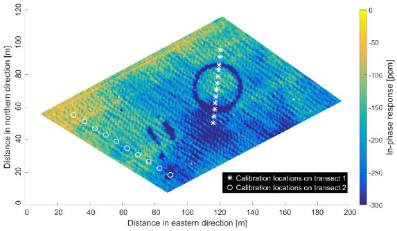
Figure 5: Subset of the field measurement data: In-phase data of the PRP 1.1 m coil, interpolated (natural-neighbour) to a 0.3$\times$0.3 m grid and corrected for offset error, signal drift and shift. Calibration data were collected along two transects.

Data from transect 1 crossing the man-made ditch structure are inverted using both the OP and IP responses of the HCP 1 m and PRP 1.1 m coil. This transect was selected for two reasons: (1) it shows a relatively wide range of response values and lateral variation, and (2) the inversion results can be validated using the calibration data as ground truth.

The prior model of the inversion is defined on 40 discretization layers, each with a thickness of 5 cm. Uniform mean and STD were set for the prior model. The value of the mean and of the STD are derived from the sample mean and sample STD of the calibration data from both transects (analogous to the procedure described for the synthetic data set). Further, the calibration data suggest only gradual vertical changes of EC and MS. For this reason, a correlation between prior model parameters was introduced with a correlation length of 5cm which is in the order of magnitude of the sampling interval of the calibration data. For the covariance matrix (eq. 9), this leads to a correlation of approximately 0.2 for the first off-diagonals and zero correlation for all subsequent off-diagonals. A forward run for 10,000 samples of the uniform prior model was carried out initially. Subsequently, the correlation between prior and forward response was computed and used as a measure for sensitivity following the approach described above (Figure 6). After visual assessment of the correlation curves, the threshold correlation for the DOI determination was set to 0.1. For EC, this yields a DOI of 0.87 m, and for MS a DOI of 0.82 m. This is in good agreement with the sensitivities as computed by the forward model following a perturbation of the calibration data [32].

The FDEM measurement ensembles for the two coils were created using the noise level of the instrument (20 ppm) as STD of the measurement PDFs [38]. Finally, EC and MS values were updated assimilating the measurements along transect 1.

The posterior best fit profiles are shown in Figure 6. Best fit EC values range from 4 to 11 mS/m. Best fit MS values are spread out over one order of magnitude (from 2$\cdot 10^{-2}$ to 1.5$\cdot 10^{-3}$). Alongside the best fit profiles, the mean STDs of the posterior PDFs (for logarithmic EC and MS values) are shown in Figure 6. The STDs indicate the uncertainty of the inversion result. Since the same prior ensemble was used for all vertical profiles, the obtained uncertainty is almost identical for each vertical profile along the transect. Therefore, only its mean value is shown in Figure 6. Possible variation in STD may occur due to the sampling differences between the measurement ensembles but this variation is small. The posterior STD is smaller than the prior STD (0.198 for EC and 0.299 for MS) at the top of the profile. With increasing profile depth the STD is rising until, near the DOI, the prior STD is reached.

As validation of the inversion result, the best fit is compared to the calibration data (Fig. 6). The general variation in EC and MS is sufficiently recovered in the best fit. As expected, we find higher EC and MS for the upper tens of centimeter. Below, EC and MS values drop. At approximately 9.5 m and 37 m distance along the transect, the ditch structure is clearly visible as highly susceptible wedges. In accordance with the calibration profiles, the ditches are less distinct in the EC profile.

Considering absolute values, MS values are systematically overestimated in the best fit. This might be explained by the severe offset errors in the raw IP signals which might not be sufficiently corrected by the comparison to the simulated forward responses of the calibration data.

Below approximately 70 cm, MS values are close to the profile mean value. This mean value is close to the mean of the MS prior model (6.1$\cdot 10^{-4}$). This is in agreement with the flattening of the IP correlation for the PRP 1.1 m coil which indicates a low sensitivity of the IP response to MS. Like the posterior mean, the posterior STD is close to the prior STD. As already observed for the synthetic data example, for lowly correlated profile sections, the inversion tends to reproduce the prior model.

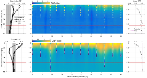
Figure 6: Left: Correlation between OP electromagnetic signal and EC (top), correlation between IP signal and MS (bottom). The depth of investigation (DOI) is indicated where correlation falls below 0.1. Center: Inversion results (best fit) for EC (top) and MS (bottom) compared to the calibration data (circles with fill color corresponding to data value). Right: Standard deviation (STD) of the prior PDFs and mean STD of the posterior PDFs for logarithmic EC (top) and logarithmic MS (bottom).

5 Conclusion

We apply the Kalman ensemble generator (KEG) in a probabilistic inversion that allows simultaneous recovery of electrical conductivity and magnetic susceptibility models from frequency-domain electromagnetic data (FDEM). Correlations between prior electrical conductivity (EC) and magnetic susceptibility (MS) ensembles and the corresponding forward response ensembles are computed during the application of the KEG. We use these correlations to estimate sensitivities of the forward responses to EC and MS. The depth of investigation is set by defining a threshold correlation. To the best of our knowledge, this is the first time that the KEG has been used for FDEM inversion. Discussing the KEG in a FDEM context is promising, especially when moving towards larger and multi-dimensional forward models. As computationally expensive forward calculations are also an issue for other types of geophysical data, we believe that interest in the presented method might not be limited to the electromagnetic community.

The KEG inversion allows to express uncertainties of prior beliefs and calibration data in a simplified Bayesian framework, as it is a Monte-Carlo implementation of a Gaussian Bayesian update problem. The avoidance of an exhaustive search of the model space makes the method more efficient than standard MCMC approaches. The error propagation in the algorithm provides a best fit to the measurement data and a measure for the uncertainty around the best fit. No additional regularization parameters are needed by the algorithm, as a trade-off the approach is restricted to modeling approximately Gaussian parameters.

The KEG proves to be efficient, particularly when identical prior models are assumed at multiple inversion locations. In such cases, and when the measurement setup is constant, we can save computational time by re-using the initial KEG ensemble for all inversions with identical prior assumptions. For the presented field data example, we re-used one initial KEG ensemble for the processing of approximately 300 neighboring inversion locations across one transect.

While in this work only prior models with a uniform mean vector and STD have been used, it is possible to define prior models with varying layer properties in order to model more heterogeneous subsurfaces. The behavior of non-uniform prior models and more sophisticated geostatistical prior correlations models can be investigated in the future.

The KEG is capable of performing parameter estimations for a large number of model parameters. The approach can be extended by adding additional parameters to the estimation: systematic errors, location of the measurement device, and dielectric permittivity estimation for high frequency applications.

References

- [1] C. von Hebel, S. Rudolph, A. Mester, J. A. Huisman, P. Kumbhar, H. Vereecken, and J. van der Kruk, “Three-dimensional imaging of subsurface structural patterns using quantitative large-scale multiconfiguration electromagnetic induction data,” Water Resources Research, vol. 50, no. 3, pp. 2732–2748, 2014.
- [2] P. De Smedt, T. Saey, A. Lehouck, B. Stichelbaut, E. Meerschman, M. M. Islam, E. Van De Vijver, and M. Van Meirvenne, “Exploring the potential of multi-receiver EMI survey for geoarchaeological prospection: A 90ha dataset,” Geoderma, vol. 199, pp. 30–36, 2013.
- [3] S. Delefortrie, T. Saey, E. Van De Vijver, P. De Smedt, T. Missiaen, I. Demerre, and M. Van Meirvenne, “Frequency domain electromagnetic induction survey in the intertidal zone: Limitations of low-induction-number and depth of exploration,” Journal of Applied Geophysics, vol. 100, pp. 14–22, 2014.
- [4] F.-X. Simon, A. Sarris, J. Thiesson, and A. Tabbagh, “Mapping of quadrature magnetic susceptibility/magnetic viscosity of soils by using multi-frequency EMI,” Journal of Applied Geophysics, vol. 120, pp. 36–47, 2015.
- [5] J. McNeill, Electromagnetic terrain conductivity measurement at low induction numbers. Geonics Limited Ontario, Canada, 1980.
- [6] W. Nowak, “Best unbiased ensemble linearization and the quasi-linear Kalman ensemble generator,” Water Resources Research, vol. 45, no. 4, 2009.
- [7] L. P. Beard and J. E. Nyquist, “Simultaneous inversion of airborne electromagnetic data for resistivity and magnetic permeability,” Geophysics, vol. 63, no. 5, pp. 1556–1564, 1998.
- [8] H. Huang and D. C. Fraser, “Airborne resistivity and susceptibility mapping in magnetically polarizable areas,” Geophysics, vol. 65, no. 2, pp. 502–511, 2000.
- [9] Y. Sasaki, J.-H. Kim, and S.-J. Cho, “Multidimensional inversion of loop-loop frequency-domain EM data for resistivity and magnetic susceptibility,” Geophysics, vol. 75, no. 6, pp. F213–F223, 2010.
- [10] C. G. Farquharson, D. W. Oldenburg, and P. S. Routh, “Simultaneous 1D inversion of loop–loop electromagnetic data for magnetic susceptibility and electrical conductivity,” Geophysics, vol. 68, no. 6, pp. 1857–1869, 2003.
- [11] R. Aster, B. Borchers, and C. Thurber, Parameter estimation and inverse problems. Elsevier Academic, 2005.
- [12] B. J. Minsley, “A trans-dimensional Bayesian Markov chain Monte Carlo algorithm for model assessment using frequency-domain electromagnetic data,” Geophysical Journal International, vol. 187, no. 1, pp. 252–272, 2011.
- [13] G. Evensen, “The ensemble Kalman filter: Theoretical formulation and practical implementation,” Ocean dynamics, vol. 53, no. 4, pp. 343–367, 2003.
- [14] M. E. Everett, Near-surface applied geophysics. Cambridge University Press, 2013.
- [15] D. Hanssens, S. Delefortrie, J. De Pue, M. Van Meirvenne, and P. De Smedt, “Frequency-domain electromagnetic forward and sensitivity modeling: Practical aspects of modeling a magnetic dipole in a multilayered half-space,” IEEE Geoscience and Remote Sensing Magazine, vol. 7, no. 1, pp. 74–85, 2019.
- [16] S. H. Ward and G. W. Hohmann, “Electromagnetic theory for geophysical applications,” Electromagnetic methods in applied geophysics, vol. 1, no. 3, pp. 131–311, 1988.
- [17] D. Guptasarma and B. Singh, “New digital linear filters for Hankel J0 and J1 transforms,” Geophysical prospecting, vol. 45, no. 5, pp. 745–762, 1997.
- [18] M. Allmaras, W. Bangerth, J. M. Linhart, J. Polanco, F. Wang, K. Wang, J. Webster, and S. Zedler, “Estimating parameters in physical models through Bayesian inversion: a complete example,” SIAM Review, vol. 55, no. 1, pp. 149–167, 2013.
- [19] A. Tarantola, Inverse problem theory and methods for model parameter estimation. SIAM, 2005.
- [20] R. E. Kalman, “A new approach to linear filtering and prediction problems,” Journal of basic Engineering, vol. 82, no. 1, pp. 35–45, 1960.
- [21] G. Evensen, “Sequential data assimilation with a nonlinear quasi-geostrophic model using Monte Carlo methods to forecast error statistics,” Journal of Geophysical Research: Oceans, vol. 99, no. C5, pp. 10143–10162, 1994.
- [22] H. Hendricks Franssen and W. Kinzelbach, “Real-time groundwater flow modeling with the ensemble Kalman filter: Joint estimation of states and parameters and the filter inbreeding problem,” Water Resources Research, vol. 44, no. 9, 2008.
- [23] H. Zhou, J. J. Gomez-Hernandez, H.-J. H. Franssen, and L. Li, “An approach to handling non-Gaussianity of parameters and state variables in ensemble Kalman filtering,” Advances in Water Resources, vol. 34, no. 7, pp. 844–864, 2011.
- [24] A. Gelman, H. S. Stern, J. B. Carlin, D. B. Dunson, A. Vehtari, and D. B. Rubin, Bayesian data analysis. Chapman and Hall/CRC, 2013.
- [25] K. Mardia, J. Kent, and J. Bibby, Multivariate analysis. Academic Press, London, 1979.
- [26] T. M. Hansen, A. G. Journel, A. Tarantola, and K. Mosegaard, “Linear inverse Gaussian theory and geostatistics,” Geophysics, vol. 71, no. 6, pp. R101–R111, 2006.
- [27] A. Tarantola and B. Valette, “Generalized nonlinear inverse problems solved using the least squares criterion,” Reviews of Geophysics, vol. 20, no. 2, pp. 219–232, 1982.
- [28] G. Gaspari and S. E. Cohn, “Construction of correlation functions in two and three dimensions,” Quarterly Journal of the Royal Meteorological Society, vol. 125, no. 554, pp. 723–757, 1999.
- [29] G. de Pasquale and N. Linde, “On structure-based priors in Bayesian geophysical inversion,” Geophysical Journal International, vol. 208, no. 3, pp. 1342–1358, 2016.
- [30] D. W. Oldenburg and Y. Li, “Estimating depth of investigation in DC resistivity and IP surveys,” Geophysics, vol. 64, no. 2, pp. 403–416, 1999.
- [31] A. Christiansen and E. Auken, “A global measure for depth of investigation,” Geophysics, vol. 77, no. 4, pp. WB171–WB177, 2012.
- [32] P. McGillivray and D. Oldenburg, “Methods for calculating Fréchet derivatives and sensitivities for the non-linear inverse problem: A comparative study,” Geophysical Prospecting, vol. 38, no. 5, pp. 499–524, 1990.
- [33] S. Delefortrie, D. Hanssens, and P. De Smedt, “Low signal-to-noise FDEM in-phase data: Practical potential for magnetic susceptibility modelling,” Journal of Applied Geophysics, vol. 152, pp. 17–25, 2018.
- [34] S. Delefortrie, T. Saey, J. De Pue, E. Van De Vijver, P. De Smedt, and M. Van Meirvenne, “Evaluating corrections for a horizontal offset between sensor and position data for surveys on land,” Precision agriculture, vol. 17, no. 3, pp. 349–364, 2016.
- [35] S. Delefortrie, P. De Smedt, T. Saey, E. Van De Vijver, and M. Van Meirvenne, “An efficient calibration procedure for correction of drift in EMI survey data,” Journal of Applied Geophysics, vol. 110, pp. 115–125, 2014.
- [36] P. De Smedt, S. Delefortrie, and F. Wyffels, “Identifying and removing micro-drift in ground-based electromagnetic induction data,” Journal of Applied Geophysics, vol. 131, pp. 14–22, 2016.
- [37] B. J. Minsley, B. D. Smith, R. Hammack, J. I. Sams, and G. Veloski, “Calibration and filtering strategies for frequency domain electromagnetic data,” Journal of Applied Geophysics, vol. 80, pp. 56–66, 2012.
- [38] DUALEM, DUALEM-421S User’s Manual. Dualem Inc., 2013.