Dynamics of curved travelling fronts for the discrete Allen-Cahn equation on a two-dimensional lattice

Abstract

In this paper we consider the discrete Allen-Cahn equation posed on a two-dimensional rectangular lattice. We analyze the large-time behaviour of solutions that start as bounded perturbations to the well-known planar front solution that travels in the horizontal direction. In particular, we construct an asymptotic phase function $\gamma_{j}(t)$ and show that for each vertical coordinate $j$ the corresponding horizontal slice of the solution converges to the planar front shifted by $\gamma_{j}(t)$. We exploit the comparison principle to show that the evolution of these phase variables can be approximated by an appropriate discretization of the mean curvature flow with a direction-dependent drift term. This generalizes the results obtained in [46] for the spatially continuous setting. Finally, we prove that the horizontal planar wave is nonlinearly stable with respect to perturbations that are asymptotically periodic in the vertical direction.

… , , [coraut]Corresponding author. [LD1] Mathematisch Instituut - Universiteit Leiden
P.O. Box 9512; 2300 RA Leiden; The Netherlands
Email: m.jukic@math.leidenuniv.nl [LD2] Mathematisch Instituut - Universiteit Leiden
P.O. Box 9512; 2300 RA Leiden; The Netherlands
Email: hhupkes@math.leidenuniv.nl

34K31 37L15.

Travelling waves, bistable reaction-diffusion systems, spatial discretizations, discrete curvature flow, nonlinear stability, modified Bessel functions of the first kind.

1 Introduction

Our main aim in this paper is to explore the large time behaviour of the Allen-Cahn lattice differential equation (LDE)

$$\dot{u}_{i,j}=u_{i+1,j}+u_{i-1,j}+u_{i,j+1}+u_{i,j-1}-4u_{i,j}+g(u_{i,j};a)$$ (1.1)

posed on the planar lattice $(i,j)\in\mathbb{Z}^{2}$. The nonlinearity $g(\cdot;a)\in C^{2}({\mathbb{R}})$ is of bistable type, in the sense that it has two stable equilibria at $u=0$ and $u=1$ and one unstable equilibrium at $u=a\in(0,1)$. The prototypical example is the cubic

$$g_{\mathrm{cub}}(u;a)=u(1-u)(u-a).$$ (1.2)

We are interested in the stability properties of curved versions of the horizontal travelling front

$$u_{i,j}(t)=\Phi(i-ct),\qquad\Phi(-\infty)=0,\qquad\Phi(+\infty)=1$$ (1.3)

in the case where $c\neq 0$. In particular, for initial conditions that are $j$-uniformly ‘front-like’ in the sense

$$\limsup_{i\to-\infty}\sup_{j\in{\mathbb{R}}}u_{i,j}(0)<a,\qquad\qquad\liminf_{i\to\infty}\inf_{j\in{\mathbb{R}}}u_{i,j}(0)>a,$$ (1.4)

we establish the uniform convergence

$$u_{i,j}(t)\to\Phi\big{(}i-\gamma_{j}(t)\big{)},\qquad t\to\infty,$$ (1.5)

for some appropriately constructed transverse phase variables $\gamma_{j}(t)$. In addition, we show that the evolution of these phases can be approximated by a discrete version of the mean curvature flow.

After adding further restrictions to (1.4), a detailed analysis of this curvature flow allows us to establish the convergence $\gamma_{j}(t)\to ct+\mu$. In fact, it turns out that the set of initial conditions covered by this result is significantly broader than the sets considered in earlier work [30, 29]. As a consequence, we widen the known basin of attraction for the planar horizontal wave (1.3).

Continuous setting The LDE (1.1) can be seen as a discrete analogue of the two-dimensional Allen-Cahn PDE

$$u_{t}=u_{xx}+u_{yy}+g(u;a).$$ (1.6)

Our primary interest here is in planar travelling travelling front solutions

$$u(x,y,t)=\Phi(x\cos\theta+y\sin\theta-ct)$$ (1.7)

that connect the two stable equilibria, in the sense that the waveprofile $\Phi$ satisfies

$$\lim_{\xi\to-\infty}\Phi(\xi)=0,\qquad\qquad\lim_{\xi\to\infty}\Phi(\xi)=1.$$ (1.8)

Direct substitution shows that the wave $(\Phi,c)$ must satisfy the $\theta$-independent ODE

$$-c\Phi^{\prime}(\xi)=\Phi^{\prime\prime}(\xi)+g\big{(}\Phi(\xi);a\big{)},$$ (1.9)

reflecting the rotational symmetry of (1.6). Indeed, (1.9) also arises as the wave ODE for the one-dimensional counterpart

$$u_{t}=u_{xx}+g(u;a).$$ (1.10)

of (1.6). The existence of solutions to (1.9) can be obtained via phase-plane analysis [24] for any parameter $a\in(0,1)$. Moreover, the pair $(\Phi,c)$ is unique up to translations, depends smoothly on the parameter $a$, and admits the strict monotonicity $\Phi^{\prime}>0$.

Modelling background

Reaction-diffusion equations have been used as modelling tools in many different fields. For example, the classical papers [3, 4] use both one- and multi-dimensional versions of such equations to describe the expression of genes throughout a population. Bistable nonlinearities such as (1.2) are typically used to model the strong Allee effect - a biological phenomenon which arises in the field of the population dynamics [54]. Indeed, the parameter $a$ can be seen as a type of minimum viability threshold that a population needs to reach in order to grow, in contrast to the standard logistic dynamics. Adding the ability for the population to diffuse throughout its spatial habitat results in systems such as (1.6) [53]. In this setting, travelling waves provide a mechanism by which species can invade (or withdraw from) the spatial domain.

In many applications this spatial domain has a discrete structure, in which case it is more natural to consider the LDE (1.1). For example, in [41, 39] the authors use this LDE to study populations in patchy landscapes. This allows them to describe and analyze a so-called ‘invasion pinning’ scenario, wherein a species fails to propagate as a direct consequence of the spatial discreteness.

By now, models involving LDEs have appeared in many other scientific and technological fields. For example, they have been used to describe phase transitions in Ising models [7], nerve pulse propagation in myelinated axons [9, 10, 37, 38], calcium channels dynamics [5], crystal growth in materials [14] and wave propagation through semiconductors [15]. For a more extensive list we recommend the surveys [19, 17, 33].

Stability of PDE waves

The first stability result for the wave (1.7) in the one-dimensional setting of (1.10) was established by Fife and McLeod in [25]. In particular, they showed that this wave (and its translates) attracts all solutions $u$ with initial conditions that satisfy

$$\limsup_{x\to-\infty}u(x,0)<a,\qquad\qquad\liminf_{x\to+\infty}u(x,0)>a,$$ (1.11)

together with $u(\cdot,0)\in[0,1]$. This latter restriction was later weakened to $u(\cdot,0)\in L^{\infty}({\mathbb{R}})$ in [23]. Both these proofs rely on the construction of super- and sub-solutions for (1.10) in order to exploit the comparison principle for parabolic equations. More recently, similar large-basin stability results have been obtained using variational methods that do not appeal to the comparison principle [26, 49].

In [36], Kapitula established the multidimensional stability of traveling waves in $H^{k}({\mathbb{R}}^{n})$, for $n\geq 2$ and $k\geq\lfloor\frac{n+1}{2}\rfloor$. These results were recently extended by Zeng [57], who considered perturbations in $L^{\infty}({\mathbb{R}}^{n})$. An alternate stability proof exploiting the comparison principle can be found in the seminal paper [13], where the authors study the interaction of travelling fronts with compact obstacles. Let us also mention the pioneering works [56, 40] which contain the first stability results for $n\geq 4$ together with partial results for $n=2,3$.

Based on the techniques developed by Kapitula, Roussier [50] was able to consider ‘asymptotically spherical’ waves and establish their stability under spherically symmetric perturbations. Such solutions behave as

$$u(x,y,t)\to\Phi\Big{(}\sqrt{x^{2}+y^{2}}-ct-c^{-1}\ln t\Big{)},\qquad\qquad t\to\infty$$ (1.12)

and were first studied by Uchiyama and Jones [35, 55]. Note that the extra time dependence highlights the important role that curvature-driven effects have to play.

Curved PDE fronts

Our work in the present paper is inspired heavily by the results for (1.6) obtained by Matano and Nara in [46]. They considered bounded initial conditions satisfying the limits

$$\limsup_{x\to-\infty}\sup_{y\in{\mathbb{R}}}u_{0}(x,y)<a,\quad\liminf_{x\to\infty}\inf_{y\in{\mathbb{R}}}u_{0}(x,y)>a,$$ (1.13)

which form the natural two-dimensional generalization of (1.11). They show that eventually horizontal cross-sections of $u$ become sufficiently monotonic to allow a phase $\gamma=\gamma(y,t)$ to be uniquely defined by the requirement

$$u\big{(}\gamma(y,t),y,t\big{)}=\Phi(0).$$ (1.14)

These phase variables can be used to characterize the asymptotic behaviour of $u$. In particular, the authors establish the limit

$$\lim_{t\to\infty}\sup_{(x,y)\in{\mathbb{R}}^{2}}|u(x,y,t)-\Phi\big{(}x-\gamma(y,t)\big{)}|=0$$ (1.15)

and show that - asymptotically - the phase $\gamma$ closely tracks solutions $\Gamma$ to the PDE

$$\dfrac{\Gamma_{t}}{\sqrt{1+\Gamma_{y}^{2}}}=\dfrac{\Gamma_{yy}}{(1+\Gamma_{y}^{2})^{3/2}}+c.$$ (1.16)

Upon supplementing (1.13) with the requirement that the initial condition $u(\cdot,\cdot,0)$ is uniquely ergodic in the $x$-direction, a careful analysis of (1.16) can be used to show that $\gamma(y,t)\to ct+\mu$ for some $\mu\in{\mathbb{R}}$. This can hence be interpreted as a stability result for the planar waves (1.7) under a large class of non-localized perturbations. Note however that no information is provided on the rate at which the convergence takes place. Very recently - and simultaneously with our analysis here - Matano, Mori and Nara generalized this approach to consider radially expanding surfaces in anistropic continuous media [45].

Mean curvature flow

In order to interpret the PDE (1.16), we consider the interfacial graph $G(t):=\left\{(\Gamma(y,t),y):y\in{\mathbb{R}}\right\}$. Writing $\nu(y,t)$ for the rightward-pointing normal vector, $V(y,t)$ for the horizontal velocity vector and $H(y,t)$ for the curvature at the point $(\Gamma(y,t),y)$, we obtain

$$\nu=\big{[}1+\Gamma_{y}^{2}\big{]}^{-1/2}(1,-\Gamma_{y}),\qquad\qquad V=(\Gamma_{t},0\big{)},\qquad\qquad H=\big{[}1+\Gamma_{y}^{2}\big{]}^{-3/2}\Gamma_{yy}.$$ (1.17)

In particular, (1.16) can be written in the form

$$V\cdot\nu=H+c,$$ (1.18)

which can be interpreted as a mean curvature flow with an additional normal drift of size $c$. It is no coincidence that this drift does not depend on $\nu$: it reflects the fact that the speed of the planar waves (1.7) does not depend on the angle $\theta$.

In a sense, it is not too surprising that the mean curvature flow plays a role in the asymptotic dynamics of wave interfaces. Indeed, one of the main historical reasons for considering the Allen-Cahn PDE is that it actually desingularizes this flow by smoothing out the transition region [1, 21]. However, from a technical point of view, its role in [46] is actually rather minor.

Instead, the main PDE used to capture the behaviour of the phase $\gamma$ is the nonlinear heat equation

$$V_{t}=V_{yy}+\dfrac{c}{2}V_{y}^{2}+c.$$ (1.19)

This PDE can be reformulated as a standard linear heat equation by a Cole-Hopf transformation and hence explicitly solved. These solutions can subsequently be used to construct super- and sub-solutions to (1.6) of the form

$$u^{\pm}(x,y,t)=\Phi\left(\dfrac{x-V(y,t)}{\sqrt{1+V_{y}^{2}}}\pm q(t)\right)\pm p(t),$$ (1.20)

in which $q$ and $p$ are small correction terms that allow spatially homogeneous perturbations at $t=0$ to be traded off for phase-shifts as $t\to\infty$.

Using the comparison principle, one can use the functions (1.20) to show that the phase $\gamma$ can be approximated asymptotically by $V$. A second comparison principle argument subsequently shows that $V$ can be used to track the solution $\Gamma$ of (1.16). It therefore plays a crucial role as an intermediary to obtain the desired relation between $\gamma$ and $\Gamma$.

Spatially discrete travelling waves

Plugging the travelling wave ansatz

$$u_{ij}(t)=\Phi(i\cos\theta+j\sin\theta-ct),\qquad\qquad\Phi(-\infty)=0,\qquad\Phi(+\infty)=1$$ (1.21)

into the Allen-Cahn LDE (1.1), we obtain the functional differential equation of mixed type (MFDE)

$$-c\Phi^{\prime}(\xi)=\Phi(\xi+\cos\theta)+\Phi(\xi-\cos\theta)+\Phi(\xi+\sin\theta)+\Phi(\xi-\sin\theta)-4\Phi(\xi)+g\big{(}\Phi(\xi);a\big{)}.$$ (1.22)

The existence of such waves $(\Phi_{\theta},c_{\theta})$ was first obtained for the horizontal direction $\theta=0$ [28, 59] and subsequently generalized to arbitrary directions [43]. This $\theta$-dependence is a direct consequence of the anistropy of the lattice, which breaks the rotational symmetry of the PDE (1.6).

A second important difference between (1.9) and (1.22) is that the character of the latter system depends crucially on the speed $c$, which depends uniquely but intricately on the parameters $(\theta,a)$. When $c\neq 0$ the associated waveprofile is unique up to translation and satisfies $\Phi^{\prime}>0$. When $c=0$ however, one loses the uniqueness and smoothness of waveprofiles. In addition, monotonic and non-monotonic profiles typically coexist. This behaviour is a direct consequence of the fact that (1.22) reduces to a difference equation, posed on a discrete ($\tan\theta\in\mathbb{Q}$) or dense ($\tan\theta\notin\mathbb{Q}$) subset of ${\mathbb{R}}$. The transition between these two regimes is a highly interesting and widely studied topic, focusing on themes such as propagation failure [34, 31, 37], crystallographic pinning [44, 31] and frictionless kink propagation [6, 22]; see [33] for an overview.

For the remainder of the present paper we only consider the case $c\neq 0$ and shift our attention to the stability properties of the associated waves. In one spatial dimension Zinner obtained the first stability result [58], which was followed by the development of a diverse set of tools exploiting either the comparison principle [16], monodromy operators [18] or spatial-temporal Green’s functions [8, 51]. The first stability result in two spatial dimensions was obtained in [29] for waves travelling in arbitrary rational ($\tan\theta\in\mathbb{Q}$) directions. Taking $\theta=0$ here for presentation purposes, the authors consider initial conditions of the form

$$u_{i,j}(0)=\Phi(i)+v^{0}_{i,j}$$ (1.23)

and show that $u$ converges algebraically to the horizontal wave $\Phi(i-ct)$. Here the initial perturbation $v^{0}$ is taken to be sufficiently small in $\ell^{\infty}\big{(}\mathbb{Z};\ell^{1}(\mathbb{Z};{\mathbb{R}})\big{)}$. In particular, the perturbation $v^{0}$ is only required to be localized in the direction perpendicular to the wave propagation.

The restriction $\tan\theta\in\mathbb{Q}$ was removed in the sequel paper [30], where the initial perturbation $v^{0}$ in (1.23) can be of arbitrary size as long as it is localized in the sense that

$$\lim_{|i|+|j|\to\infty}|v^{0}_{i,j}|=0.$$ (1.24)

The proof relies on the construction of explicit sub- and super-solutions to the LDE (1.1), generalizing the PDE constructions from [12]. This construction is especially delicate for the cases $\theta\notin\frac{\pi}{4}\mathbb{Z}$, where the disalignment with the lattice directions causes slowly decaying modes that need to be carefully controlled.

Curved LDE fronts

In order to avoid the problematic slowly decaying terms discussed above, we restrict ourselves to the horizontal waves (1.3) throughout the remainder of the paper. The novelty is that we allow general bounded initial conditions that satisfy the limits (1.4). To compare this with the discussion above, we note that this class includes initial conditions of the form

$$u_{i,j}(0)=\Phi\big{(}i-\kappa_{j}\big{)}+v^{0}_{i,j},$$ (1.25)

in which $\kappa$ is an arbitrary bounded sequence and $v^{0}$ is allowed to be small in $\ell^{\infty}\big{(}\mathbb{Z};\ell^{1}(\mathbb{Z};{\mathbb{R}})\big{)}$ or to satisfy the localization condition (1.24). In particular, we significantly expand the set of initial conditions that were considered in [29, 30].

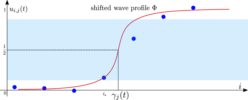
Our main aim is to follow the program of [46] that we outlined above as closely as possible. However, the first obstacle already arises when one attempts to define appropriate phase coordinates $\gamma_{j}(t)$ for $t\gg 1$. Indeed, it no longer makes sense to define the interface of $u(t)$ as the set of points where $u_{i,j}(t)=\Phi(0)$, since this solution set can behave highly erratically due to the discreteness of the spatial variables. To resolve this, we establish an asymptotic monotonicity result in the interfacial region where $u_{i,j}(t)\approx\Phi(0)$. This allows us to ‘fill’ the troublesome gaps between lattice points by performing a spatial interpolation based on the shape of $\Phi$; see Fig. 1.

Figure 1: In §5 we show that for each $j\in\mathbb{Z}$ and $t\gg 0$, the function $i\mapsto u_{i,j}(t)$ is monotonic inside an interfacial region $I$ that is depicted in light blue. The dark blue dots represent the horizontal solution slice $i\mapsto u_{i,j}(t)$. Since $u$ is monotonic inside $I$, we can find an unique value $i_{*}$ for which $u_{i_{*},j}(t)\leq 1/2<u_{i_{*}+1,j}(t)$. We subsequently shift the travelling wave profile $\Phi$ in such a way that it matches the solution slice at $i_{*}$. The phase $\gamma_{j}(t)$ is then defined as the argument where this shifted profile equals one half.

This fundamental problem of not being able to move continuously between lattice points occurs in many other parts of our analysis. For example, we need to construct so-called $\omega$-limit points of solution sequences in order to establish the uniform convergence (1.5). In [46] this is achieved by passing to a new coordinate $x^{\prime}=x-ct$ that ‘freezes’ the wave at the cost of an extra convective term in the PDE (1.6). Such a coordinate transformation does not exist in the discrete case, forcing us to use a more involved discontinuous version of this freezing process.

Discrete curvature flow

We remark that it is by no means a-priori clear how the mean curvature PDE (1.16) should be discretized in order to track the discrete phase coordinates $\gamma_{j}(t)$. For example, there is more than one reasonable way to define geometric notions such as normal vectors and curvature in discrete settings [20]. On the other hand, the discussion above shows that there may be range of ‘suitable’ choices, as we only desire the tracking to be approximate.

Introducing the convenient notation

$$[\beta_{\Gamma}]_{j}=\sqrt{1+\dfrac{(\Gamma_{j+1}-\Gamma_{j})^{2}+(\Gamma_{j-1}-\Gamma_{j})^{2}}{2}},\qquad\qquad[\partial^{(2)}\Gamma]_{j}=\Gamma_{j+1}+\Gamma_{j-1}-2\Gamma_{j},$$ (1.26)

we will use the standard symmetric discretizations

$$V\cdot\nu\mapsto\beta_{\Gamma}^{-1}\dot{\Gamma},\qquad\qquad H\mapsto\beta_{\Gamma}^{-3}\partial^{(2)}\Gamma$$ (1.27)

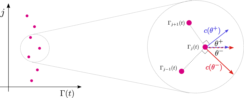
for the normal velocity and curvature terms in (1.18). However, the remaining normal drift term requires more care to account for the direction dependence of the planar front speeds. In particular, it seems natural make the replacement

$$c\mapsto\frac{1}{2}\big{(}c_{\theta^{+}}+c_{\theta^{-}}\big{)},$$ (1.28)

in which the angles

$$\theta^{-}=\arctan{(\Gamma_{j}-\Gamma_{j-1})},\qquad\qquad\theta^{+}=\arctan{(\Gamma_{j+1}-\Gamma_{j})}$$ (1.29)

measure the orientation of the normal vectors for the lower and upper segments of the interface at $(\Gamma_{j},j)$; see Fig. 2.

Figure 2: The panel on the left represents a graph $j\mapsto\Gamma_{j}(t)$ at a fixed time $t$. The right panel zooms in on three nodes of this graph to illustrate the identities (1.28) and (1.29) that underpin the drift term in our discrete curvature flow.

In order to make this more explicit, we use the identity $[\partial_{\theta}c_{\theta}]_{\theta=0}=0$ derived in [32, Lem. 2.2] to obtain the expansions

$$c_{\theta_{-}}\sim c+\dfrac{1}{2}[\partial_{\theta}^{2}c_{\theta}]_{\theta=0}(\Gamma_{j}-\Gamma_{j-1})^{2},\qquad\qquad c_{\theta_{+}}\sim c+\dfrac{1}{2}[\partial_{\theta}^{2}c_{\theta}]_{\theta=0}(\Gamma_{j+1}-\Gamma_{j})^{2},$$ (1.30)

which suggests the replacement

$$c\mapsto c+\dfrac{1}{2}[\partial_{\theta}^{2}c_{\theta}]_{\theta=0}\big{(}\beta_{\Gamma}^{2}-1\big{)}.$$ (1.31)

In order to prevent the quadratic growth in this term, we make the final adjustment

$$c\mapsto c+[\partial_{\theta}^{2}c_{\theta}]_{\theta=0}\big{(}1-\beta_{\Gamma}^{-1}\big{)},$$ (1.32)

which agrees with (1.31) up to second order in the differences $\Gamma_{j\pm 1}-\Gamma_{j}$.

All in all, the discrete mean curvature flow that we use in this paper to approximate the phases $\gamma_{j}$ can be written as

$$\beta_{\Gamma}^{-1}\dot{\Gamma}=\beta_{\Gamma}^{-3}\partial^{(2)}\Gamma+c+[\partial_{\theta}^{2}c_{\theta}]_{\theta=0}\big{(}1-\beta_{\Gamma}^{-1}\big{)}.$$ (1.33)

While this justification appears to be rather ad-hoc, it turns out that our approximation procedure is not sensitive to $O\big{(}(\Gamma_{j\pm 1}-\Gamma_{j})^{3}\big{)}$-correction terms. In addition, we explain below how the crucial lower order terms can be recovered by independent technical considerations.

Super- and sub-solutions

The technical heart of this paper is formed by our construction of suitable spatially discrete versions of the sub- and super-solutions (1.20). The correct generalization of (1.19) that preserves the Cole-Hopf structure turns out to be

$$\dot{V}_{j}=\dfrac{1}{d}\left(e^{d(V_{j+1}-V_{j})}-2+e^{d(V_{j-1}-V_{j})}\right)+c,$$ (1.34)

in which we are still free to pick the coefficient $d$. Indeed, this LDE reduces to the discrete heat equation upon picking $h(t)=e^{d(V-ct)}$.

However, the discrete Laplacian spawns terms proportional to $\Phi^{\prime\prime}(\beta_{V}^{2}-1)$ if one simply substitutes a direct discretization of the PDE super-solution (1.20) with (1.34) into (1.1). These terms decay as $O(t^{-1})$ and hence cannot be integrated and absorbed into the phaseshift $q(t)$.

Similar difficulties were also encountered in [30]. The novelty here is that this troublesome behaviour occurs even for the horizontal direction $\theta=0$, which is completely aligned with the lattice. Inspired by the normal form approach developed in [30], we therefore set out to construct sub- and super-solutions of the form

$$u^{\pm}_{i,j}(t)=\Phi\big{(}i-V_{j}(t)\pm q(t)\big{)}+r\big{(}i-V_{j}(t)\pm q(t)\big{)}([\beta_{V}]_{j}^{2}-1)\pm p(t),$$ (1.35)

using the extra residual function $r$ to neutralize the slowly decaying terms. Working through the computations, it turns out the relevant condition on the pair $(r,d)$ can be formulated as

$$\mathcal{L}_{\mathrm{tw}}r+d\Phi^{\prime}=-\Phi^{\prime\prime},$$ (1.36)

in which the Fredholm operator $\mathcal{L}_{\mathrm{tw}}$ encodes the linearization of the wave MFDE (1.22) around $\Phi$; see §7. Using the Fredholm theory for MFDEs developed in [42, 43] together with the computations in §8 and [32, §2], it turns out that $d$ must be given by

$$d=\frac{1}{2}c+\frac{1}{2}[\partial_{\theta}^{2}c_{\theta}]_{\theta=0}=\frac{1}{2}\big{[}\partial^{2}_{\theta}\mathcal{D}(\theta)\big{]}_{\theta=0},$$ (1.37)

in which the quantity

$$\mathcal{D}(\theta)=\frac{c_{\theta}}{\cos\theta}$$ (1.38)

is referred to as the directional dispersion. This quantity measures the horizontal speed of waves travelling in the direction $\theta$, which also plays an important role in the construction of travelling corner solutions to (1.1).

(a)

(b)

Figure 3: Both panels illustrate front-like initial conditions that satisfy (1.4) and hence fall within the framework of this paper. Panel a) provides an example of an initial perturbation that converges uniformly to a traveling front. On the contrary, the initial perturbation in b) does not uniformly converge to a traveling planar front, but the evolution of the interface is described asymptotically by (1.33).

Stability results

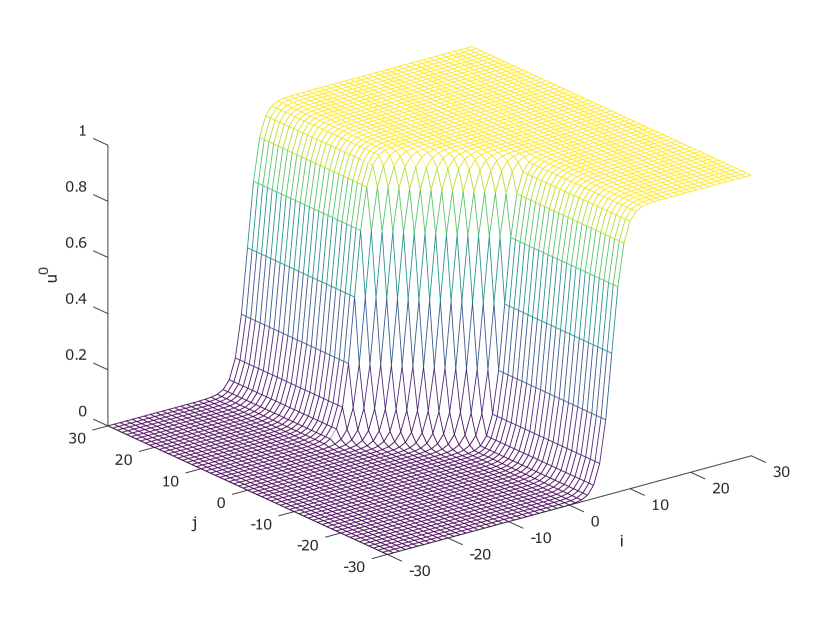
As a by-product of our analysis, we are able to extend the stability results obtained previously in [29, 30]. For example, if the phase sequence $\kappa$ appearing in the initial condition (1.25) is periodic (see e.g. Fig. 3(a)), we show that there exists an asymptotic phase $\mu\in{\mathbb{R}}$ for which we have the convergence $\gamma(t)\to ct+\mu$ as $t\to\infty$. In particular, the horizontal planar wave retains its stability under such perturbations, provided we allow for a phase-shift.

In order to prove this result, we first analyze the behaviour of (1.1) and (1.34) when applied to $j$-periodic sequences. We subsequently add a localized initial perturbation and show that the effects remain localized in some sense. Since the heat-equation eventually eliminates such localized perturbations, the desired asymptotic convergence persists. We remark that our stability result is slightly less general than its continuous counterpart from [46], since it is not yet clear to us how ergodicity properties can be transferred to our discrete setting.

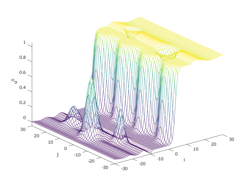
We emphasize that this stability result does not hold for arbitrary bounded $\kappa$ in (1.25). For example, if there exist $\kappa^{-}$ and $\kappa^{+}$ for which we have the limits

$$\lim_{j\to-\infty}\kappa_{j}=\kappa^{-},\qquad\qquad\lim_{j\to+\infty}\kappa_{j}=\kappa^{+}$$ (1.39)

(see e.g. Fig. 3(b)), then the results in §9 imply that for every $t>0$ we have the convergence

$$u_{i,j}(t)\to\Phi(i-ct-\kappa^{\pm})\quad\ \text{as}\ j\to\pm\infty,$$ (1.40)

uniformly in $i$. In particular, the interface $\gamma(t)$ describes the phase transition between $\kappa^{-}$ and $\kappa^{+}$, which is asymptotically captured by (1.33).

Organization

After formulating our assumptions and main results in §2, we transfer the standard $\omega$-limit point constructions for the PDE (1.6) to our discrete setting in §3. In §4 we (partially) generalize the results from [11] concerning trapped entire solutions to the setting of (1.1). In particular, we prove that every entire solution of the Allen-Cahn LDE trapped between two traveling waves is a traveling wave itself. In §5 we focus on the large-time behaviour of the solution $u$ and establish the discrete counterpart of (1.15). We move on in §6 to obtain decay estimates for discrete gradients of solutions to the discrete heat equation. We exploit these in §7 to construct super- and sub-solutions, which we use in §8 to approximate the phase $\gamma$ with the solution of the discrete mean curvature flow (1.33). Finally, in §9 we establish the stability results discussed above for the horizontal planar travelling wave.

Acknowledgments

Both authors acknowledge support from the Netherlands Organization for Scientific Research (NWO) (grant 639.032.612).

2 Main results

Our principal interest in this paper is the discrete Allen-Cahn equation

$$\dot{u}_{i,j}=(\Delta^{+}u)_{i,j}+g(u_{i,j})$$ (2.1)

posed on the planar lattice $(i,j)\in\mathbb{Z}^{2}$. The discrete Laplacian $\Delta^{+}:\ell^{\infty}(\mathbb{Z}^{2})\to\ell^{\infty}(\mathbb{Z}^{2})$ is defined as

$$(\Delta^{+}u)_{i,j}=u_{i+1,j}+u_{i,j+1}+u_{i-1,j}+u_{i,j-1}-4u_{i,j},$$ (2.2)

while the nonlinearity is assumed to satisfy the following bistability condition.

• The nonlinear function $g:{\mathbb{R}}\to{\mathbb{R}}$ is $C^{2}$-smooth and there exists $a\in(0,1)$ for which we have

  $$g(0)=g(a)=g(1)=0,\qquad g^{\prime}(0)<0,\qquad g^{\prime}(1)<0.$$ (2.3)

  In addition, we have the inequalities

  $$g>0\text{ on }(-\infty,0)\cup(a,1),\qquad\qquad g<0\text{ on }(0,a)\cup(1,\infty).$$ (2.4)

Existence results for planar traveling wave solutions of (2.1) were established in [43]. More precisely, if we pick an arbitrary angle $\theta\in[0,2\pi)$, then (2.1) admits a solution of the form

$$u_{ij}(t)=\Phi_{\theta}(i\cos\theta+j\sin\theta-c_{\theta}t),$$ (2.5)

for some wave speed $c_{\theta}\in{\mathbb{R}}$ and wave profile $\Phi_{\theta}:{\mathbb{R}}\to{\mathbb{R}}$ that satisfies the boundary conditions

$$\lim_{\xi\to-\infty}\Phi_{\theta}(\xi)=0,\quad\lim_{\xi\to+\infty}\Phi_{\theta}(\xi)=1.$$ (2.6)

Substituting the Ansatz (2.5) into (2.1), we see that the the pair $(\Phi_{\theta},c_{\theta})$ must satisfy the MFDE

$$-c_{\theta}\Phi_{\theta}^{\prime}(\xi)=\Phi_{\theta}(\xi+\cos\theta)+\Phi_{\theta}(\xi+\sin\theta)+\Phi_{\theta}(\xi-\cos\theta)+\Phi_{\theta}(\xi-\sin\theta)-4\Phi_{\theta}(\xi)+g\big{(}\Phi_{\theta}(\xi)\big{)}.$$ (2.7)

The results in [43] state that $c_{\theta}$ is unique. In addition, when $c_{\theta}\neq 0$, the wave profile $\Phi_{\theta}$ is unique up to translation and satisfies $\Phi^{\prime}_{\theta}>0$. In this paper, we are interested in planar waves that travel in the horizontal direction $\theta=0$. Since we rely on smoothness properties of the wave profile, we demand that $c_{0}\neq 0$.

• There exists a non-zero speed $c\neq 0$ and a wave profile $\Phi\in C^{1}({\mathbb{R}},{\mathbb{R}})$ so that the pair $(\Phi,c)$ satisfies the boundary conditions (2.6) and the MFDE (2.7) for the horizontal direction $\theta=0$. In addition, we have the normalization $\Phi(0)=\frac{1}{2}$.

Our main results concern the Cauchy problem for the Allen-Cahn LDE. In particular, we look for functions

$$u\in C^{1}\big{(}[0,\infty);\ell^{\infty}(\mathbb{Z}^{2})\big{)}$$ (2.8)

that satisfy the LDE (2.1) for $t>0$ together with the initial condition

$$u_{i,j}(0)=u^{0}_{i,j}$$ (2.9)

for some $u^{0}\in\ell^{\infty}(\mathbb{Z}^{2})$. Observe that the comparison principle together with the bistable structure of $g$ imply that such solutions are unique and exist globally. We impose the following structural condition on $u^{0}$.

• The initial condition $u^{0}\in\ell^{\infty}(\mathbb{Z}^{2})$ satisfies the inequalities

  $$\limsup_{i\to-\infty}\sup_{j\in\mathbb{Z}}u^{0}_{i,j}<a,\quad\qquad\liminf_{i\to\infty}\inf_{j\in\mathbb{Z}}u^{0}_{i,j}>a.$$ (2.10)

Notice that we do not impose the usual assumption $0\leq u^{0}\leq 1$ or any kind of decay in the spatial limits. As explained in detail in §1, this condition is less restrictive than its counterparts from [29, 30] and includes the general class (1.25).

2.1 Interface formation

Our first goal is to find a link between the solution (2.8) of the general Cauchy problem for (2.1) and the planar travelling wave $(\Phi,c)$. The result below provides a key tool for this purpose when $t\gg 1$. In particular, it establishes that for each fixed $j\in\mathbb{Z}$, the horizontal slice $i\mapsto u_{ij}(t)$ ‘crosses through’ the value $u=\frac{1}{2}$ in a monotonic fashion.

Proposition 2.1 (see §5).

There exists a time $T>0$ such that for every $j\in\mathbb{Z}$ and $t\geq T$ there exists a unique $i_{*}=i_{*}(j,t)$ with the property

$$0<u_{i_{*},j}(t)\leq\dfrac{1}{2},\quad u_{i_{*}+1,j}(t)>\dfrac{1}{2}.$$ (2.11)

These functions $i(j,t)$ can be used to define a set of phases $\big{(}\gamma_{j}(t)\big{)}_{j\in\mathbb{Z}}$ that measure in some sense where the value $u=\frac{1}{2}$ is ‘crossed’. More precisely, we define a function $\gamma:[T,\infty)\to\ell^{\infty}(\mathbb{Z})$ that acts as

$$\gamma_{j}(t)=i_{*}(j,t)-\Phi^{-1}\big{(}u_{i_{*}(j,t),j}(t)\big{)};$$ (2.12)

see Fig. 1. The motivation behind the second term on the right is our desire to recover the traditional phase when $u$ is itself a travelling wave. Indeed, in the special case that

$$u_{i,j}(t)=\Phi(i-ct-\mu)$$ (2.13)

for some $\mu\in{\mathbb{R}}$, the phase condition $\Phi(0)=\frac{1}{2}$ implies that

$$i_{*}(j,t)=\lfloor ct+\mu\rfloor.$$ (2.14)

In particular, we obtain

$$\gamma_{j}(t)=ct+\mu,$$ (2.15)

which allows us to write

$$u_{i,j}(t)=\Phi\big{(}i-\gamma_{j}(t)\big{)}.$$ (2.16)

The drawback of this relatively straightforward construction is that the phases $\gamma_{j}(t)$ will in general admit discontinuities. However, the size of these jumps will tend to zero as $t\to\infty$, which suffices for our asymptotic purposes.

Our main result here is that this phase description (2.16) holds asymptotically for any initial condition $u^{0}$ that satisfies (H0). In particular, for large time, the dynamics of the full solution $u$ can be approximated by the behaviour of the phase coordinates $\gamma(t)$.

Theorem 2.2 (see §5).

Suppose that (Hg), $(H\Phi)$ and (H0) are satisfied and consider the solution $u$ of the discrete Allen-Cahn equation (2.1) with the initial condition (2.9). Then we have the limit

$$\lim_{t\to\infty}\sup_{(i,j)\in\mathbb{Z}^{2}}\big{|}u_{i,j}(t)-\Phi\big{(}i-\gamma_{j}(t)\big{)}\big{|}=0.$$ (2.17)

2.2 Interface evolution

Our second main goal is to uncover the long-term dynamics of the phase $\gamma$ defined in (2.12). In particular, we show that this evolution can be approximated by a discrete version of the mean curvature flow with an appropriate drift term.

In order to formulate this equation, we pick a sequence $\Gamma\in\ell^{\infty}(\mathbb{Z})$ and introduce the discrete derivatives

$$\begin{array}[]{lcl}[\partial^{+}\Gamma]_{j}&=&\Gamma_{j+1}-\Gamma_{j},\\[5.69046pt] [\partial^{-}\Gamma]_{j}&=&\Gamma_{j}-\Gamma_{j-1},\\[5.69046pt] [\partial^{(2)}\Gamma]_{j}&=&\Gamma_{j+1}-2\Gamma_{j}+\Gamma_{j-1},\end{array}$$ (2.18)

together with the sequence

$$[\beta_{\Gamma}]_{j}=\sqrt{1+\dfrac{1}{2}(\partial^{+}\Gamma)^{2}_{j}+\dfrac{1}{2}(\partial^{-}\Gamma)^{2}_{j}}.$$ (2.19)

As explained in §1, the driving force in (2.21) below is not a constant as in the PDE case. Instead, it features additional terms that arise due to the underlying anisotropy of the lattice.

Theorem 2.3 (see §8).

Suppose that (Hg), $(H\Phi)$ and (H0) are all satisfied, consider the solution $u$ of the LDE (2.1) with the initial condition (2.9) and recall the phase $\gamma$ defined in (2.12). Then for every $\epsilon>0$, there exists $\tau_{\epsilon}\geq T$ so that for any $\tau\geq\tau_{\epsilon}$, the solution

$$\Gamma:[\tau,\infty)\to\ell^{\infty}(\mathbb{Z})$$ (2.20)

to the initial value problem

$$\left\{\begin{array}[]{lcl}\beta_{\Gamma}^{-1}\dot{\Gamma}&=&\beta_{\Gamma}^{-3}\partial^{(2)}\Gamma+\left(c+[\partial_{\theta}^{2}c_{\theta}]_{\theta=0}\right)-\beta_{\Gamma}^{-1}[\partial_{\theta}^{2}c_{\theta}]_{\theta=0}\\[5.69046pt] \Gamma(\tau)&=&\gamma(\tau)\end{array}\right.$$ (2.21)

satisfies the estimate

$$\sup_{t\geq\tau}\left|\left|{\Gamma(t)-\gamma(t)}\right|\right|_{\ell^{\infty}}<\epsilon.$$ (2.22)

Our final result provides more detailed information on the asymptotics of $\gamma$ in the special case that the initial condition $u^{0}$ is a localized perturbation from a front-like background state that is periodic in $j$. Indeed, this provides sufficient control on (2.21) to show that the corresponding solution converges to a planar travelling front. We emphasize that the case $P=1$ encompasses the stability results from [29, 30], albeit only for horizontal waves.

Theorem 2.4 (see §9).

Suppose that (Hg), (H$\Phi$) and (H0) are satisfied and consider the solution $u$ of the discrete Allen-Cahn equation (2.1) with the initial condition (2.9). Suppose furthermore that there exists a sequence $u^{0;\mathrm{per}}\in\ell^{\infty}(\mathbb{Z}^{2})$ so that the following two properties hold.

• We have the limit

  $$u^{0}_{i,j}-u^{0;\mathrm{per}}_{i,j}\to 0,\quad\text{as}\quad|i|+|j|\to\infty.$$ (2.23)

• There exists an integer $P\geq 1$ so that

  $$u^{0;\mathrm{per}}_{i,j+P}=u^{0;\mathrm{per}}_{i,j},\qquad\qquad\hbox{ for all }(i,j)\in\mathbb{Z}^{2}.$$ (2.24)

Then there exists a constant $\mu\in{\mathbb{R}}$ for which we have the limit

$$\lim_{t\to\infty}\sup_{(i,j)\in\mathbb{Z}^{2}}|u_{i,j}(t)-\Phi(i-ct-\mu)|=0.$$ (2.25)

3 Omega limit points

The techniques used in [46] relied heavily upon the ability to construct so-called omega limit points. More specifically, consider a solution $u:{\mathbb{R}}^{2}\times[0,\infty)\to{\mathbb{R}}$ to the PDE (1.6) together with an unbounded sequence $0<t_{1}<t_{2}<\ldots$ and a set of vertical shifts $(y_{k})\subset{\mathbb{R}}$. One can then establish [46] the existence of an entire solution $\omega$ to (1.6) for which the convergence

$$u(x+ct_{k},y+y_{k},t+t_{k})\to\omega(x,y,t)\quad\text{ in }C_{\text{loc}}^{2,1}({\mathbb{R}}^{2}\times{\mathbb{R}})$$ (3.1)

holds as $k\to\infty$, possibly after passing to a subsequence. This can be achieved efficiently by replacing $x$ with the travelling wave coordinate $x-ct$.

Any direct attempt to generalize this procedure to the LDE setting will fail on account of the fact that $i-ct$ is not necessarily an integer. Indeed, this prevents us from introducing a well-defined co-moving frame. Our approach here to handle this is rather crude: we simply round the horizontal shifts upward towards the nearest integer.

To illustrate this, let us consider the planar wave solution

$$u_{ij}(t)=\Phi(i-ct)$$ (3.2)

together with an unbounded sequence $0<t_{1}<t_{2}<\ldots$ and a set of vertical shifts $(j_{k})\subset\mathbb{Z}$. Possibly taking a subsequence, we obtain the convergence

$$[0,1]\ni\lceil ct_{k}\rceil-ct_{k}\to\theta_{\omega}$$ (3.3)

as $k\to\infty$, which means that

$$u_{i+\lceil ct_{k}\rceil,j+j_{k}}(t+t_{k})=\Phi(i+\lceil ct_{k}\rceil-ct-ct_{k})\to\Phi(i-ct+\theta_{\omega})$$ (3.4)

as $k\to\infty$. In particular, we do still recover an entire solution, at the price of a small phase-shift that would not occur in the continuous framework. As we will see throughout the following sections, this phase-shift does not cause any qualitative difficulties.

Our main result confirms that our procedure indeed generates $\omega$-limit points. In addition, it states that such limits are trapped between two travelling waves, which turns out to be a crucial point in our analysis. The consequences of this fact will be discussed in greater depth in §4.

Proposition 3.1.

Suppose that (Hg), $(H\Phi)$ and (H0) are satisfied. Let $u\in C^{1}\big{(}[0,\infty);\ell^{\infty}(\mathbb{Z}^{2})\big{)}$ be a solution of the LDE (2.1). Then for any sequence $(j_{k},t_{k})$ in $\mathbb{Z}\times[0,\infty)$ with $0<t_{1}<t_{2}<\dots\to\infty$, there exists a subsequence $(j_{n_{k}},t_{n_{k}})$ and a function $\omega\in C^{1}\big{(}{\mathbb{R}};\ell^{\infty}(\mathbb{Z}^{2})\big{)}$ with the following properties.

1. We have the convergence

   $$u_{i+\lceil ct_{n_{k}}\rceil,j+j_{n_{k}}}(t+t_{n_{k}})\to\omega_{i,j}(t)\quad\text{ in }C_{\mathrm{loc}}(\mathbb{Z}^{2}\times{\mathbb{R}})$$ (3.5)

   as $k\to\infty$.

2. The limit $\omega$ satisfies the discrete Allen-Cahn equation (2.1) on $\mathbb{Z}^{2}\times{\mathbb{R}}$.

3. There exists a constant $\theta\in{\mathbb{R}}$ such that

   $$\Phi(i-ct-\theta)\leq\omega_{i,j}(t)\leq\Phi(i-ct+\theta),\quad\text{for all }i\in\mathbb{Z}\text{ and }t\in{\mathbb{R}}.$$ (3.6)

We refer to such a function $\omega$ as an $\omega$-limit point of the solution $u$. The proof of the bounds (3.6) relies on the fact that the LDE (2.1) admits a comparison principle; see [30, Prop. 3.1]. In order to exploit this, we introduce the residual

$$\mathcal{J}[u]=\dot{u}-\Delta^{+}u-f(u)$$ (3.7)

and recall that a function

$$u\in C^{1}\big{(}[0,\infty);\ell^{\infty}(\mathbb{Z}^{2})\big{)}$$ (3.8)

is referred to as a sub- or super-solution to the discrete Allen-Cahn equation (2.1) if $\mathcal{J}[u]_{i,j}(t)\leq 0$ respectively $\mathcal{J}[u]_{i,j}(t)\geq 0$ holds for all $t\geq 0$ and $(i,j)\in\mathbb{Z}^{2}$. Our first result describes a standard pair of such solutions, using the well-known principle that uniform perturbations to the travelling wave $\Phi$ at $t=0$ can be traded off for phase-shifts at $t=\infty$.

Lemma 3.2.

Assume that (H$g$) and (H$\Phi$) are satisfied. Then for any $q_{0}\in(0,a)$ and $q_{1}\in(0,1-a)$, there exist constants $\mu>0$ and $C\geq 1$ so that the functions

$$u^{+}_{i,j}(t) =\Phi\left(i-ct+Cq_{0}(1-e^{-\mu t})\right)+q_{0}e^{-\mu t},$$ (3.9)

$$u^{-}_{i,j}(t) =\Phi\left(i-ct-Cq_{1}(1-e^{-\mu t})\right)-q_{1}e^{-\mu t}$$ (3.10)

are a super- respectively sub-solution of the discrete Allen-Cahn equation (2.1).

Proof.

The arguments from Lemma 4.1 in [25] can be copied almost verbatim; see for example [16]. ∎

We now turn to the solution $u$ of the LDE (2.1) with the initial condition (2.9). Using two a-priori estimates we will show that $u$ can eventually be controlled by time translates of $u^{+}$ and $u^{-}$. By exploiting the divergence $t_{k}\to\infty$ of the time-shifts for the $\omega$-limit point, we can subsequently eliminate the uniform additive terms in (3.9)-(3.10) and recover the phase-shifts in (3.6).

Lemma 3.3.

Assume that (H$g$) and (H0) are satisfied. Pick $q_{0}\in(0,a)$ in such a way that the initial condition $u^{0}$ satisfies

$$\limsup_{i\to-\infty}\sup_{j\in\mathbb{Z}}u^{0}_{i,j}<q_{0}.$$

Then for every $t>0$ we have the bound

$$\limsup_{i\to-\infty}\sup_{j\in\mathbb{Z}}u_{i,j}(t)<q_{0}.$$ (3.11)

Proof.

First, we find a constant $d\in(0,q_{0})$ for which

$$\limsup_{i\to-\infty}\sup_{j\in\mathbb{Z}}u^{0}_{i,j}<d.$$ (3.12)

Next, we pick a constant $M$ in such a way that

$$u^{0}_{i,j}\leq d+Me^{i|c|},\quad\text{for every }(i,j)\in\mathbb{Z}^{2}.$$ (3.13)

Writing $K>0$ for the maximum value of the function $g$ on the interval $[a,1]$, we choose $\alpha>0$ sufficiently large to have

$$\alpha|c|-\dfrac{c^{4}}{12}\cosh|c|\geq\dfrac{2K}{a-d}.$$ (3.14)

We now claim that the $j$-independent function

$$w_{i,j}(t)=d+Me^{|c|(i+|c|t+\alpha t)}$$ (3.15)

is a super-solution to (2.1). To see this, we compute

$$\mathcal{J}[w]_{i,j}(t) =Me^{|c|(i+|c|t+\alpha t)}\left(c^{2}+\alpha|c|-e^{-|c|}-e^{|c|}+2\right)-g\big{(}w_{i,j}(t)\big{)}$$

$$=Me^{|c|(i+|c|t+\alpha t)}\left(\alpha|c|-\dfrac{c^{4}}{12}\cosh\tilde{c}\right)-g\big{(}w_{i,j}(t)\big{)}$$

$$\geq\big{(}w_{i,j}(t)-d\big{)}\frac{2K}{a-d}-g\big{(}w_{i,j}(t)\big{)},$$

where $\tilde{c}$ is a number between $0$ and $|c|$. For $w_{i,j}(t)\in[0,a]\cup[1,\infty)$, we have $g\big{(}w_{i,j}(t)\big{)}\leq 0$, which immediately gives $\mathcal{J}[w]_{i,j}(t)\geq 0$. On the other hand, for $w_{i,j}(t)\in[a,1]$ our choice for $K$ yields

$$\mathcal{J}[w]_{i,j}(t)\geq(a-d)\dfrac{2K}{a-d}-K\geq K>0.$$

Applying the comparison principle we conclude

$$u_{i,j}(t)\leq w_{i,j}(t)=d+Me^{|c|(i+|c|t+\alpha t)},\quad$$ (3.16)

$\text{for every }t\geq 0\ \text{and }(i,j)\in\mathbb{Z}^{2}$. Taking the supremum over $j\in\mathbb{Z}$ and sending $i$ to $-\infty$ we obtain the desired inequality (3.11). ∎

Lemma 3.4.

Suppose that (Hg), $(H\Phi)$ and (H0) are satisfied. Let $u$ be the solution of the discrete Allen-Cahn equation (2.1) with the initial condition (2.9). Then for every $q_{0}>0$ there exists $T>0$ so that

$$u_{i,j}(t)\leq 1+\dfrac{q_{0}}{2}$$ (3.17)

holds for every $t\geq T$ and $(i,j)\in\mathbb{Z}^{2}$.

Proof.

Let $\tilde{u}$ be the solution to the scalar initial value problem

$$\begin{cases}\tilde{u}_{t}&=g(\tilde{u}),\qquad t>0\\ \tilde{u}(0)&=\left|\left|{u^{0}}\right|\right|_{\ell^{\infty}(\mathbb{Z}^{2})}.\\ \end{cases}$$ (3.18)

Since $g(u)<0$ for all $u>1$, there exists $T>0$ such that $\tilde{u}(t)\leq 1+\frac{q_{0}}{2}$ for all $t\geq T$. Exploiting the fact that $\tilde{u}$ is also a spatially homogeneous solution to (2.1), the comparison principle yields $u_{i,j}(t)\leq\tilde{u}(t)$ for all $t\geq 0$ and $(i,j)\in\mathbb{Z}^{2}$. Combining these observations leads directly to (3.17). ∎

Lemma 3.5.

Assume that (Hg), $(H\Phi)$ and (H0) are satisfied. Then there exists a time $T>0$ together with constants

$$q_{0}\in(0,a),\qquad q_{1}\in(0,1-a),\qquad\theta_{0}\in{\mathbb{R}},\qquad\theta_{1}\in{\mathbb{R}},\qquad\mu>0,\qquad C>0$$ (3.19)

so that the solution $u$ to (2.1) with the initial condition (2.9) satisfies the estimates

$$u_{i,j}(t)\leq\Phi\left(i+\theta_{0}-c(t-T)+Cq_{0}\big{(}1-e^{-\mu(t-T)}\big{)}\right)+q_{0}e^{-\mu(t-T)},\quad\forall t\geq T,$$ (3.20)

$$u_{i,j}(t)\geq\Phi\left(i-\theta_{1}-c(t-T)-Cq_{1}\big{(}1-e^{-\mu(t-T)}\big{)}\right)-q_{1}e^{-\mu(t-T)},\quad\forall t\geq T.$$ (3.21)

Proof.

We first choose $q_{0}\in(0,a)$ in such a way that

$$\limsup_{i\to-\infty}\sup_{j\in\mathbb{Z}}u^{0}_{i,j}<q_{0}.$$ (3.22)

Using Lemma 3.4, we obtain $T>0$ for which

$$u_{i,j}(T)\leq 1+\dfrac{q_{0}}{2}\quad\text{for every }(i,j)\in\mathbb{Z}^{2}.$$ (3.23)

On the other hand, Lemma 3.3 allows us to find $\vartheta_{a}\in\mathbb{Z}$ so that

$$u_{i,j}(T)\leq q_{0},\quad\text{for }i\leq\vartheta_{a}\text{ and}\ j\in\mathbb{Z}.$$ (3.24)

Finally, in view of the limits  (2.6) there exists $\vartheta_{b}\in\mathbb{Z}$ for which

$$\Phi(i)\geq 1-\frac{q_{0}}{2},\quad\text{for every }i\geq\vartheta_{b}.$$

Combining these inequalities and recalling the definition (3.9), we obtain

$$u_{i,j}(T)\leq\Phi(i-\vartheta_{a}+\vartheta_{b})+q_{0}=u_{i-\vartheta_{a}+\vartheta_{b}}^{+}(0)$$ (3.25)

for all $i\in\mathbb{Z}$. The desired upper bound (3.20) with $\theta_{0}=\vartheta_{b}-\vartheta_{a}$ now follows from Lemma 3.2 and the comparison principle. The lower bound can be obtained in a similar fashion.

∎

Proof of Proposition 3.1.

Fix an integer $L\in{\mathbb{N}}$ and consider the functions

$$u^{k}\in C\big{(}[-L,L];{\mathbb{R}}^{(2L+1)\times(2L+1)}\big{)}$$

that are defined by

$$u^{k}_{i,j}(t)=u_{i+\lceil ct_{n_{k}}\rceil,j+j_{n_{k}}}(t+t_{n_{k}}),\quad\quad(i,j,t)\in\{-L,\ldots,L\}^{2}\times[-L,L]$$

for all sufficiently large $k$. Lemma 3.4 implies that the solution $u$ and hence the functions $u^{k}$ are globally bounded. Since the derivative $\dot{u}$ satisfies (2.1), it follows that $\dot{u}^{k}$ is also a globally bounded sequence. Hence, Ascoli-Arzela implies that the sequence $u^{k}$ is relatively compact. By using a standard diagonalization argument together with (2.1), we obtain a subsequence $u^{n_{k}}$ and a function $\omega:{\mathbb{R}}\to\ell^{\infty}(\mathbb{Z}^{2})$ so that

$$\sup_{(i,j,t)\in K}|u^{n_{k}}_{i,j}(t)-\omega_{i,j}(t)|+|\dot{u}^{n_{k}}_{i,j}(t)-\dot{\omega}_{i,j}(t)|\to 0,$$

for every compact $K\subset\mathbb{Z}^{2}\times{\mathbb{R}}$. This immediately implies (i) and (ii). The bounds (3.6) follow directly from Lemma 3.5. ∎

4 Trapped entire solutions

The main point of this section is to prove that every entire solution that is trapped between two traveling waves is a traveling wave itself. This is a very useful result when combined with Proposition  3.1, since it implies that every $\omega$-limit point of the solution $u$ is a traveling wave. This will turn out to be a crucial tool during our analysis of the large time behaviour of $u$.

Proposition 4.1.

Assume that (H$g$) and (H$\Phi$) are satisfied and consider a function $\omega\in C^{1}\big{(}{\mathbb{R}};\ell^{\infty}(\mathbb{Z}^{2})\big{)}$ that satisfies the Allen-Cahn LDE (2.1) for all $t\in{\mathbb{R}}$. Assume furthermore that there exists a constant $\theta$ for which the bounds

$$\Phi(i-ct-\theta)\leq\omega_{i,j}(t)\leq\Phi(i-ct+\theta)$$ (4.1)

hold for all $(i,j)\in\mathbb{Z}^{2}$ and $t\in{\mathbb{R}}$. Then there exists a constant $\theta_{0}\in[-\theta,\theta]$ so that

$$\omega_{i,j}(t)=\Phi(i-ct-\theta_{0}),\quad\hbox{for all }(i,j)\in\mathbb{Z}^{2},\,t\in{\mathbb{R}}.$$

This result is a generalization of [11, Thm. 3.1] to the current spatially discrete setting. The main complication lies in the fact that the LDE (2.1) is a nonlocal equation, as opposed to the PDE (1.6). For example, if a smooth function $f:E\subset{\mathbb{R}}^{2}\to{\mathbb{R}}$ attains a local minimum at some point $x_{0}$, then we automatically have $\Delta f(x_{0})\geq 0$. This is an important ingredient for the arguments in [11], but fails to hold in our spatially discrete setting.

Indeed, if $v\in\ell^{\infty}(\mathbb{Z}^{2})$ attains a minimum in $E\subset\mathbb{Z}^{2}$ at some point $(i,j)\in E$, it does not automatically follow that the discrete Laplacian satisfies $(\Delta^{+}v)_{i,j}\geq 0$. This conclusion can only be obtained if one can verify that the nearest neighbours of $(i,j)$ are also contained in $E$. This is the key purpose of our first technical result.

Lemma 4.2.

Consider the setting of Proposition 4.1 and pick a sufficiently small $\delta>0$. Choose a pair $(I,J)\in\mathbb{Z}^{2}$ together with a constant $\sigma\in{\mathbb{R}}$. Suppose for some $\kappa\in\mathbb{Z}$ that the function

$$v^{\sigma}_{i,j}(t)=\omega_{i+I,j+J}\left(t+\dfrac{I}{c}+\dfrac{\sigma}{c}\right)$$ (4.2)

satisfies the inequality

$$v^{\sigma}_{i,j}(t)\leq\omega_{i,j}(t)$$ (4.3)

whenever $i-ct\in[\kappa,\kappa+1]$. Then the following claims holds true.

1. If $\omega_{i,j}(t)\geq 1-\delta$ whenever $i-ct\geq\kappa$, then in fact (4.3) holds for all $i-ct\geq\kappa$.

2. If $v^{\sigma}_{i,j}(t)\leq\delta$ whenever $i-ct\leq\kappa+1$, then in fact (4.3) holds for all $i-ct\leq\kappa+1$.

Proof.

Starting with (i), we define the set

$$E:=\left\{(i,j,t)\in\mathbb{Z}^{2}\times{\mathbb{R}}:i-ct\geq\kappa\right\}.$$

Since both functions $\omega$ and $v^{\sigma}$ are globally bounded, the quantity

$$\epsilon^{*}=\inf\left\{\epsilon>0:v^{\sigma}\leq\omega+\epsilon\text{ in }E\right\}$$

is finite. In addition, by continuity we have

$$v^{\sigma}\leq\omega+\epsilon^{*}\quad\text{in }E.$$ (4.4)

To prove the claim, it suffices to show that $\epsilon^{*}=0$. Assuming to the contrary that $\epsilon^{*}>0$, we can find sequences $\epsilon_{n}\nearrow\epsilon^{*}$ and $(i_{n},j_{n},t_{n})$ in $E$ with the property that

$$\omega_{i_{n},j_{n}}(t_{n})+\epsilon_{n}<v^{\sigma}_{i_{n},j_{n}}(t_{n})\leq\omega_{i_{n},j_{n}}(t_{n})+\epsilon^{*}\quad\text{for each }n\in{\mathbb{N}}.$$ (4.5)

Sending $n\to\infty$ we conclude that

$$\lim_{n\to\infty}\omega_{i_{n},j_{n}}(t_{n})-v^{\sigma}_{i_{n},j_{n}}(t_{n})+\epsilon^{*}=0.$$ (4.6)

Now, notice that the assumption (4.1) and the inequality $\epsilon^{*}>0$ imply that the sequence $l_{n}:=i_{n}-ct_{n}$ is bounded. In addition, our assumption (4.3) implies that $l_{n}>\kappa+1$. In particular, we can assume that the bounded sequence $i_{n}-\lceil ct_{n}\rceil$ is equal to an integer $L\geq\kappa$.

Applying Proposition 3.1 to the function $\omega$ and the sequence $(j_{n},t_{n})$, we obtain a limiting function $\omega^{\infty}$ for which we have

$$\lim_{n\to\infty}\omega_{i+\lceil ct_{n}\rceil,j+j_{n}}(t+t_{n})=\omega^{\infty}_{i,j}(t),$$ (4.7)

for each $(i,j,t)\in\mathbb{Z}^{2}\times{\mathbb{R}}$. By construction it also holds that

$$\lim_{n\to\infty}v^{\sigma}_{i+\lceil ct_{n}\rceil,j+j_{n}}(t+t_{n})=\omega^{\infty}_{i+I,j+J}(t+\dfrac{I}{c}+\dfrac{\sigma}{c}).$$ (4.8)

Next we define the function $z=z_{i,j}(t)$ as

$$z_{i,j}(t)=\omega^{\infty}_{i,j}(t)-\omega^{\infty}_{i+I,j+J}(t+\dfrac{I}{c}+\dfrac{\sigma}{c})+\epsilon^{*}.$$ (4.9)

For $(i,j,t)\in E$ we have $(i+\lceil ct_{n}\rceil,j+j_{n},t+t_{n})\in E$. Combining this with the fact that the inequality (4.4) survives the limit (4.7), we have $z_{i,j}(t)\geq 0$ in $E$. By (4.6) we obtain $z_{L,0}(0)=0$. Also, for $i-ct=\kappa$, we have $(i+\lceil ct_{n}\rceil,j+j_{n},t+t_{n})\in[\kappa,\kappa+1]$. In particular, we find

$$z_{i,j}(t)\geq\epsilon^{*}>0,\quad\text{for }i-ct=\kappa.$$ (4.10)

Therefore, it must hold that $L\geq\kappa+1$.

We pick $\delta$ to be small enough so that $g$ is non-increasing on $[1-\delta,1]$. Since $\omega^{\infty}\in[1-\delta,1]$ and $g$ is locally Lipschitz continuous on $E$, there exists $B>0$ so that

$$\dot{z}_{i,j}(t)-(\Delta^{+}z)_{i,j}(t) =g\big{(}\omega^{\infty}_{i,j}(t)\big{)}-g\big{(}\omega^{\infty}_{i+I,j+J}(t+\dfrac{I}{c}+\dfrac{\sigma}{c})\big{)}$$ (4.11)

$$\geq g(\omega^{\infty}_{i,j}(t)+\epsilon^{*})-g\big{(}\omega^{\infty}_{i+I,j+J}(t+\dfrac{I}{c}+\dfrac{\sigma}{c})\big{)}$$

$$\geq-Bz_{i,j}(t)$$

for all $(i,j,t)\in E$. Since $z$ attains its minimum at the point $(L,0,0)\in E$ with $L\geq\kappa+1$, we have $\dot{z}_{L,0}(0)=0$. In addition, the inequality $(\Delta^{+}z)_{L,0}(0)\geq 0$ holds since all the nearest neighbours of $(L,0,0)$ are contained in $E$. In particular, we compute

$$0\leq\dot{z}_{L,0}(0)-(\Delta^{+}z)_{L,0}(0)+Bz_{L,0}(0)=-(\Delta^{+}z)_{L,0}(0)\leq 0.$$ (4.12)

Therefore, $(\Delta^{+}z)(0)_{L,0}=0$ must hold, which implies that $z_{0,L-1}(0)=0$.

If $L=\kappa+1$ then we are done, since $z\geq\epsilon^{*}>0$ for $i-ct=\kappa$ which contradicts (4.10). On the other hand, if $L-1\geq\kappa+1$ we can iteratively decrease $L$ using this procedure until we reach the desired contradiction. Statement (ii) can be obtained in a similar fashion using $\lfloor ct_{n}\rfloor$ instead of $\lceil ct_{n}\rceil$. ∎

Lemma 4.3.

Consider the setting of Propostion 4.1, fix an arbitrary pair $(I,J)\in\mathbb{Z}^{2}$ and recall the functions $v^{\sigma}$ defined in (4.2) Then the quantity

$$\sigma_{*}:=\inf\left\{\sigma\in{\mathbb{R}}:v^{\tilde{\sigma}}\leq\omega\text{ in }\mathbb{Z}^{2}\times{\mathbb{R}}\text{ for all }\tilde{\sigma}\geq\sigma\right\}$$ (4.13)

satisfies $\sigma_{*}\leq 0$.

Proof.

First we show that $\sigma_{*}<\infty.$ Without loss we may assume that $0<\delta<1/2$ holds for the constant defined in Lemma 4.2. The inequalities (4.1) allow $\kappa\in{\mathbb{N}}$ such that

$$\begin{array}[]{lcll}\omega_{i,j}(t)&\geq&1-\delta,&i-ct\geq\kappa,\\[5.69046pt] \omega_{i,j}(t)&\leq&\delta,&i-ct\leq-\kappa.\end{array}$$ (4.14)

For $\sigma\geq 2\kappa+1$ and $i-ct\in\leq\kappa+1$ one has $i-ct-\sigma\leq-\kappa$. It follows from (4.14) that $v^{\sigma}\leq\delta$ on $i-ct\leq\kappa+1$. Using $\delta\leq 1-\delta$ we have $v^{\sigma}\leq\omega$ on $i-ct\in[\kappa,\kappa+1]$. Hence, both items (i) and (ii) of Lemma 4.2 are satisfied and the bound $v^{\sigma}\leq\omega$ on ${\mathbb{R}}$ follows immediately. Since $\sigma\geq 2\kappa+1$ was arbitrary, we conclude that $\sigma_{*}\leq 2\kappa+1$.

Arguing by contradiction, let us assume that $\sigma_{*}>0$. Defining the set

$$S=\left\{-\kappa-1\leq i-ct\leq\kappa+1\right\},$$ (4.15)

we now claim that

$$\inf_{S}\ (\omega-v^{\sigma_{*}})=0.$$ (4.16)

Assume to the contrary that $\inf_{S}(w-{v^{\sigma}}^{*})=K>0$. Then, using the global Lipschitz continuity of $\omega$, there exists a constant $M>0$ such that

$$\omega_{i,j}(t)-v^{\sigma_{*}-\mu}_{i,j}(t)=\omega_{i,j}(t)-v^{\sigma_{*}}_{i,j}(t)+v^{\sigma_{*}}_{i,j}(t)-v^{\sigma_{*}-\mu}_{i,j}(t)\geq K-M\mu$$ (4.17)

holds for every $\mu\geq 0$ and $(i,j,t)\in S$. Hence, there exists $\mu_{0}\in(0,\sigma_{*})$ such that $v^{\sigma_{*}-\mu}\leq\omega$ on $S$, for all $\mu\in[0,\mu_{0}]$. Item (i) in Lemma 4.2 implies that $v^{\sigma_{*}-\mu}\leq\omega$ for $i-ct\geq\kappa$ and for all $\mu\in[0,\mu_{0}]$. Furthermore, since $\sigma_{*}-\mu\geq 0$, we have $v^{\sigma_{*}-\mu}\leq\delta$ for $i-ct\leq-\kappa$. Since also $v^{\sigma_{*}-\mu}\leq\omega$ for $-\kappa-1\leq i-ct\leq-\kappa$, item (ii) of Lemma 4.2 implies that $v^{\sigma_{*}-\mu}\leq\omega$ also holds on $i-ct\leq-\kappa$. All together, we have $v^{\sigma_{*}-\mu}\leq\omega$ on $\mathbb{Z}^{2}\times{\mathbb{R}}$, which contradicts the minimality of $\sigma_{*}$ and yields (4.16).

We can hence find a sequence $(i_{n},j_{n},t_{n})$ in $S$ such that

$$\omega_{i_{n},j_{n}}(t_{n})-v^{\sigma_{*}}_{i_{n},j_{n}}(t_{n})\to 0\qquad\text{ as }n\to\infty.$$ (4.18)

Since $i_{n}-ct_{n}$ is bounded, we can assume that $i_{n}-\lceil ct_{n}\rceil$ is equal to a constant, which we denote by $L$. As before, we obtain the convergence

$$\lim_{n\to\infty}\omega_{i+\lceil ct_{n}\rceil,j+j_{n}}(t+t_{n})=\omega^{\infty}_{i,j}(t),$$ (4.19)

where $\omega^{\infty}$ is also an entire solution of the LDE (2.1). Hence, the function $z=z_{i,j}(t)$ defined as

$$z_{i,j}(t):=\omega^{\infty}_{i,j}(t)-\omega^{\infty}_{i+I,j+J}(t+\dfrac{I}{c}+\dfrac{\sigma_{*}}{c})$$ (4.20)

satisfies

$$z_{i,j}\geq 0\text{ for all }(i,j,t)\in\mathbb{Z}^{2}\times{\mathbb{R}}$$ (4.21)

and $z_{L,0}(0)=0$. Using an argument similar to the one in the proof of Lemma 4.2, it follows that $z_{i,j}(0)=0$ for all $(i,j)\in\mathbb{Z}^{2}$. We then obtain $z\equiv 0$ by the uniqueness of bounded solutions for (2.1).

In particular, we have $\omega^{\infty}_{0,0}(0)=\omega^{\infty}_{kI,kJ}(kI/c+k\sigma_{*}/c)$ for all $k\in\mathbb{Z}$. However, we also have the limits

$$\lim_{k\to-\infty}\omega^{\infty}_{kI,kJ}(kI/c+k\sigma_{*}/c)=1,\qquad\qquad\lim_{k\to\infty}\omega^{\infty}_{kI,kJ}(kI/c+k\sigma_{*}/c)=0,$$ (4.22)

since $\omega^{\infty}$ is trapped between two traveling waves as well. We have hence reached a contradiction and conclude $\sigma_{*}\leq 0$. ∎

Proof of Proposition 4.1.

From Lemma 4.3, we know that

$$\omega_{i,j}(t)\geq\omega_{i+I,j+J}(t+\dfrac{I}{c})\quad\text{on }\mathbb{Z}^{2}\times{\mathbb{R}},$$ (4.23)

for arbitrary $(I,J)\in\mathbb{Z}^{2}$. Hence, the function $\omega$ depends only on the value of $i-ct$. More precisely, there exists a function $\psi$ such that $\omega_{i,j}(t)=\psi(i-ct)$. The result now follows directly from the fact that solutions to the travelling wave problem (2.6)-(2.7) for $\theta=0$ and $c\neq 0$ are unique up to translation. ∎

5 Large time behaviour of $u$

The main goal of this section is to study the qualitative large time behaviour of the solution $u$ to our main initial value problem. In particular, we connect this behaviour to the dynamics of the phase $\gamma$ defined in (2.12) and thereby establish Theorem 2.2. In addition, we provide an asymptotic flatness result for this phase.

Our first main result concerns the large-time behaviour of the interfacial region

$$I_{t}=\left\{(i,j)\in\mathbb{Z}^{2}:\Phi(-2)\leq u_{i,j}(t)\leq\Phi(2)\right\}$$ (5.1)

where $u$ takes values close to $1/2$. For fixed $j$ and $t$, we establish that the horizontal coordinate $i$ can not jump in and out from the interface region, which is non-empty. In particular, once the map $i\mapsto u_{ij}(t)$ enters the interval $[\Phi(-2),\Phi(2)]$ from below, it cannot exit throughout the lower boundary. In addition, it is strictly increasing in $i$ and cannot reenter the interval once it has left through the upper boundary.

Proposition 5.1.

Suppose that the assumptions (Hg), (H$\Phi$) and (H0) are satisfied and let $u$ be a solution of the discrete Allen-Cahn equation (2.1) with the initial condition (2.9). Then there exists a constant $T>0$ so that the following statements are satisfied.

1. For each $t\geq T$ and $j\in\mathbb{Z}$ there exists $i\in\mathbb{Z}$ for which

   $$\Phi(-2)<u_{i,j}(t)\leq\frac{1}{2}.$$ (5.2)

2. We have the inequality

   $$\inf_{t\geq T,\,(i,j)\in I_{t}}u_{i+1,j}(t)-u_{i,j}(t)>0.$$ (5.3)

3. Consider any $t\geq T$ and $(i,j)\in\mathbb{Z}^{2}$ for which $u_{i,j}(t)\leq\Phi(-2)$ holds. Then we also have $u_{i-1,j}(t)\leq\Phi(-2)$.

4. Consider any $t\geq T$ and $(i,j)\in\mathbb{Z}^{2}$ for which $u_{i,j}(t)\geq\Phi(2)$ holds. Then we also have $u_{i+1,j}(t)\geq\Phi(2)$.

Our second main result shows that the discrete derivative of the phase with respect to $j$ tends to zero. This will turn out to be crucial in order to keep the mean curvature flow under control. We emphasize that this does not necessarily mean that the phase tends to a constant; see (1.40).

Proposition 5.2.

Consider the setting of Proposition 5.1 and recall the phase $\gamma:[T,\infty)\to\ell^{\infty}(\mathbb{Z})$ defined in (2.12). Then we have the limit

$$\lim_{t\to\infty}\sup_{j\in\mathbb{Z}}\big{|}\gamma_{j+1}(t)-\gamma_{j}(t)\big{|}=0.$$

Proof of Proposition 2.1.

The statement follows directly from Proposition 5.1. ∎

5.1 Proof of Proposition 5.1 and Theorem 2.2

The key towards establishing Proposition 5.1 is to obtain strict monotonicity properties in compact regions that move with the wavespeed $c$. This is achieved in the following result, which leverages the travelling wave identification obtained in Proposition 4.1.

Lemma 5.3.

Consider the setting of Proposition 5.1 and pick a constant $R>0$. Then there exists a constant $T>0$ such that

$$\inf_{j\in\mathbb{Z},\,|i-ct|\leq R,\,t\geq T}u_{i+1,j}(t)-u_{i,j}(t)>0.$$ (5.4)

Proof.

Arguing by contradiction, let us assume that there exists a constant $R>0$ so that

$$\inf_{j\in\mathbb{Z},\,|i-ct|\leq R,\,t\geq T}u_{i+1,j}(t)-u_{i,j}(t)\leq 0$$

holds for every $T>0$. We can then find a sequence $(t_{n},i_{n},j_{n})\in(0,\infty)\times\mathbb{Z}^{2}$ with $0<t_{1}<t_{2}<\dots\to\infty$ for which we have the inequalities

$$|i_{n}-ct_{n}|\leq R,\qquad\qquad u_{i_{n}+1,j_{n}}(t_{n})-u_{i_{n},j_{n}}(t_{n})\leq 1/n.$$ (5.5)

In particular, we may assume that the bounded sequence of integers $i_{n}-\lceil ct_{n}\rceil$ is identically equal to some constant $L\in\mathbb{Z}$. Applying Proposition 3.1 we obtain the convergence

$$u_{i+\lceil ct_{n}\rceil,j+j_{n}}(t+t_{n})\to\omega_{ij}(t)$$ (5.6)

as $n\to\infty$, in which $\omega$ is an $\omega$-limit point of the function $u$. In view of Proposition 4.1 we have $\omega_{i,j}(t)=\Phi(i-ct-\theta_{0})$ for some $\theta_{0}\in{\mathbb{R}}$, which allow us to write

$$1/n \geq u_{i_{n}+1,j_{n}}(t_{n})-u_{i_{n},j_{n}}(t_{n})$$

$$=u_{L+\lceil ct_{n}\rceil+1,j_{n}}(t_{n})-u_{L+\lceil ct_{n}\rceil,j_{n}}(t_{n})$$

$$\to\omega_{L+1,0}(0)-\omega_{L,0}(0)$$

$$=\Phi(L+1-\theta_{0})-\Phi(L-\theta_{0})$$

for $n\to\infty$. This violates the strict monotonicity $\Phi^{\prime}>0$ and hence yields the desired contradiction. ∎

Proof of Proposition 5.1.

We first prove item (iii). Assuming that this statement fails, we can find a sequence $(t_{k},i_{k},j_{k})$ for which we have $0<t_{1}<t_{2}<\ldots\to\infty$ together with the inequalities

$$u_{i_{k},j_{k}}(t_{k})\leq\Phi(-2),\qquad\qquad u_{i_{k}-1,j_{k}}(t_{k})>\Phi(-2).$$ (5.7)

It follows from Lemma 3.5 that the sequence $i_{k}-ct_{k}$ is bounded. Arguing as in the proof of Lemma 5.3, we can hence again assume that there exists $L\in\mathbb{Z}$ for which we have $L=i_{k}-\lceil ct_{k}\rceil$. In addition, we obtain the limits

$$u_{i_{k},j_{k}}(t_{k})\to\omega_{L,0}(0)\leq\Phi(-2),\qquad\qquad u_{i_{k}-1,j_{k}}(t_{k})\to\omega_{L-1,0}(0)\geq\Phi(-2).$$ (5.8)

Here $\omega$ is an $\omega$-limit point for $u$, which must be a travelling wave by Proposition 4.1. This again violates the strict monotonicity of $\Phi$. Item (iv) follows analogously.

Turning to (i), we assume that there exists a sequence $(t_{k},i_{k},j_{k})$ with $T\leq t_{1}<t_{2}<...\to\infty$ together with

$$u_{i_{k},j_{k}}(t_{k})\leq\Phi(-2),\qquad\qquad u_{i_{k}+1,j_{k}}(t_{k})>\dfrac{1}{2}=\Phi(0)$$ (5.9)

and seek a contradiction. Arguing as above, we can find $L\in\mathbb{Z}$ together with an $\omega$-limit point $\omega$ for $u$ with

$$\omega_{L,0}\leq\Phi(-2),\qquad\qquad\omega_{L+1,0}(0)\geq\Phi(0),$$ (5.10)

which violates Proposition 4.1.

It remains to establish (ii). Picking $t\geq T$ and $(i,j)\in I_{t}$, it follows from Lemma 3.5 that $i-ct$ is bounded by some constant $R$ that depends only on $T$. Increasing $T$ if necessary, we can apply Lemma 5.3 to obtain the desired bound (5.3). ∎

Lemma 5.4.

Consider the setting of Proposition 5.1 and recall the phase $\gamma:[T,\infty)\to\ell^{\infty}(\mathbb{Z})$ defined in (2.12). Then there exists $T_{*}\geq T$ and $M>0$ such that for every $t\geq T_{*}$ we have

$$\left|\left|{\gamma(t)-ct}\right|\right|_{\ell^{\infty}}\leq M.$$ (5.11)

Proof.

In view of the definition (2.12) it suffices to show that $i_{*}-ct$ is bounded. Combining Lemma 3.5 and (2.11) and possibly increasing $T>0$, we see that

$$\Phi(0)\leq u_{i_{*}(j,t)+1,j}(t)\leq\Phi\Big{(}i_{*}(j,t)+1+\theta_{0}-ct+cT+Cq_{0}(1-e^{-\mu(t-T)})\Big{)}+q_{0}e^{-\mu(t-T)}$$ (5.12)

for all $t\geq T$. Choosing $T_{*}\geq T$ in such a way that

$$\Phi(0)-q_{0}e^{-\mu(T_{*}-T)}\geq\Phi(-1),$$

we conclude that

$$i_{*}(j,t)+1+\theta_{0}-ct+cT+Cq_{0}(1-e^{-\mu(t-T)})>-1,\qquad\qquad t\geq T_{*}.$$ (5.13)

Hence, $i_{*}-ct$ is bounded from below. An upper bound can be obtained in a similar way. ∎

Proof of Theorem 2.2.

Arguing by contradiction once more, let us assume that there exist $\delta>0$ together with sequences $(i_{k},j_{k})\in\mathbb{Z}^{2}$ and $T\leq t_{1}<t_{2}<\dots\to\infty$ for which

$$|\Delta_{k}|:=|u_{i_{k},j_{k}}(t_{k})-\Phi\big{(}i_{k}-\gamma_{j_{k}}(t_{k})\big{)}|\geq\delta.$$ (5.14)

We first claim that the sequence $i_{k}-ct_{k}$ is bounded. To see this, we first use Lemma 5.4 to conclude that $\gamma_{j_{k}}(t_{k})-ct_{k}$ is bounded. Using (3.21) we subsequently find

$$\Delta_{k} \geq\Phi\big{(}i_{k}-ct_{k}+\alpha_{k}\big{)}-q_{1}e^{-\mu(t_{k}-T)}-\Phi\big{(}i_{k}-ct_{k}+\beta_{k}\big{)},$$

in which

$$\alpha_{k}=cT-\theta_{1}-Cq_{1}(1-e^{-\mu(t_{k}-T)}),\qquad\qquad\beta_{k}=ct_{k}-\gamma_{j_{k}}(t_{k})$$ (5.15)

are two bounded sequences. In particular, if $i_{k}-ct_{k}$ is unbounded we can use the exponential decay of $\Phi$ to achieve $\Delta_{k}\geq-\delta$ for all large $k$. A similar argument using (3.20) yields $\Delta_{k}\leq\delta$, which contradicts (5.14) and hence establishes our claim.

In particular, we can extract a constant subsequence $i_{k}-\lceil ct_{k}\rceil=:L\in\mathbb{Z}$. Passing to a further subsequence, we may also assume that $i_{*}(j_{k},t_{k})-\lceil ct_{k}\rceil=:\tilde{L}\in\mathbb{Z}$. The definition (2.12) allows us to write

$$\Phi\big{(}i_{k}-\gamma_{j_{k}}(t_{k})\big{)} =\Phi\Big{(}i_{k}-i_{*}(j_{k},t_{k})+\Phi^{-1}\left(u_{i_{*}(j_{k},t_{k}),j_{k}}(t_{k})\right)\Big{)}$$

$$=\Phi\Big{(}i_{k}-\lceil ct_{k}\rceil-i_{*}(j_{k},t_{k})+\lceil ct_{k}\rceil+\Phi^{-1}\left(u_{i_{*}(j_{k},t_{k}),j_{k}}(t_{k})\right)\Big{)}$$

$$=\Phi\left(L-\tilde{L}+\Phi^{-1}\big{(}u_{\tilde{L}+\lceil ct_{k}\rceil,j_{k}}(t_{k})\big{)}\right).$$

Applying Proposition 3.1, we see that there exists an $\omega$-limit point $\omega$ for $u$ for which the limits

$$u_{i_{k},j_{k}}(t_{k})\to\omega_{L,0}(0),\qquad\qquad u_{\tilde{L}+\lceil ct_{k}\rceil,j_{k}}(t_{k})\to\omega_{\tilde{L},0}(0)$$ (5.16)

hold as $k\to\infty$. Writing $\omega_{i,j}(t)=\Phi(i-ct-x_{0})$ in view of Proposition 4.1, we hence find

$$\Delta_{k}\to\Phi(L-x_{0})-\Phi\Big{(}L-\tilde{L}+\Phi^{-1}\big{(}\Phi(\tilde{L}-x_{0})\big{)}\Big{)}=0$$ (5.17)

as $k\to\infty$, which clearly contradicts (5.14). ∎

5.2 Phase asymptotics

In this subsection we shift our attention to vertical differences of the phase $\gamma$, in order to establish Proposition 5.2. Our first result resembles Lemma 5.3 in the sense that we study the interfacial region of the wave, but in this case we get a flatness result. This can subsequently be used to obtain a bound on the vertical differences of the function $i_{*}$ defined in (2.11), which in view of (2.12) allows us to analyze the phase $\gamma$.

Lemma 5.5.

Consider the setting of Proposition 5.1 and pick a constant $R>0$. Then we have the limit

$$\lim_{t\to\infty}\sup_{j\in\mathbb{Z},\,|i-ct|\leq R}|u_{i,j+1}(t)-u_{i,j}(t)|=0.$$

Proof.

Assume to the contrary that there exist constants $R>0$ and $\delta>0$ together with sequences $(i_{k},j_{k})\in\mathbb{Z}^{2}$ and $0<t_{1}<t_{2}<...\to\infty$ that satisfy the inequalities

$$|i_{k}-ct_{k}|\leq R,\qquad\qquad|u_{i_{k},j_{k}+1}(t_{k})-u_{i_{k},j_{k}}(t_{k})|\geq\delta.$$ (5.18)

As in the proof of the Lemma 5.3, we may assume that $i_{k}-\lceil ct_{k}\rceil=L\in\mathbb{Z}$ and use Proposition 3.1 to conclude the convergence

$$\begin{array}[]{lcl}u_{i_{k},j_{k}+1}(t+t_{k})-u_{i_{k},j_{n}}(t_{k})&=&u_{L+\lceil ct_{k}\rceil,j_{k}+1}(t_{k})-u_{L+\lceil ct_{k}\rceil,j_{k}}(t_{k})\\[5.69046pt] &\to&\omega_{L,1}(0)-\omega_{L,0}(0)\\[5.69046pt] &=&0,\end{array}$$ (5.19)

in which $\omega$ is an $\omega$-limit point of the function $u$. The last identity follows from Proposition 4.1, which states that $\omega$ is a planar wave travelling in the horizontal direction. This obviously contradicts (5.18) and hence concludes the proof. ∎

Lemma 5.6.

Consider the setting of Proposition 5.1 and recall the function $i_{*}$ defined by (2.11). Then there exists $\tilde{T}>T$ so that

$$|i_{*}(j+1,t)-i_{*}(j,t)|\leq 1$$ (5.20)

holds for all $j\in\mathbb{Z}$ and all $t\geq\tilde{T}$.

Proof.

If the above claim does not hold, we can find sequences $(i_{k},\tilde{i}_{k},j_{k})\in\mathbb{Z}^{3}$ and $T<t_{1}<t_{2}<\dots\to\infty$ for which the inequality $|i_{k}-\tilde{i}_{k}|>1$ holds, together with

$$\begin{cases}u_{i_{k},j_{k}}(t_{k})\leq 1/2,\\ u_{i_{k}+1,j_{k}}(t_{k})>1/2,\end{cases}\qquad\qquad\qquad\qquad\qquad\begin{cases}u_{\tilde{i}_{k},j_{k}+1}(t_{k})\leq 1/2,\\ u_{\tilde{i}_{k}+1,j_{k}+1}(t_{k})>1/2.\end{cases}$$ (5.21)

As before, we can assume that $i_{k}+\lceil ct_{k}\rceil=L\in\mathbb{Z}$ and $\tilde{i}_{k}+\lceil ct_{k}\rceil=\tilde{L}\in\mathbb{Z}$. In addition, we can use Proposition 3.1 to construct an $\omega$-limit point $\omega$ for $u$ that satisfies the inequalities

$$\begin{cases}\omega_{L,0}(0)\leq 1/2,\\ \omega_{L+1,0}(0)>1/2,\end{cases}\qquad\qquad\qquad\qquad\qquad\quad\begin{cases}\omega_{\tilde{L},1}(0)\leq 1/2,\\ \omega_{\tilde{L}+1,1}(0)>1/2\end{cases}$$ (5.22)

on account of (5.21). Therefore, Proposition 4.1 shows that the bounds

$$L\leq\theta_{0}\leq L+1,\qquad\qquad\tilde{L}\leq\theta_{0}\leq\tilde{L}+1$$

hold for some $\theta_{0}\in{\mathbb{R}}$. This allows us to conclude that $|L-\tilde{L}|\leq 1$ and obtain the contradiction $|i_{k}-\tilde{i}_{k}|\leq 1$. ∎

Proof of Proposition 5.2.

Assume to the contrary that there exists $\delta>0$ together with subsequences $(j_{k})\in\mathbb{Z}$ and $T\leq t_{1}<t_{2}<\dots\to\infty$ for which

$$|\gamma_{j_{k}+1}(t_{k})-\gamma_{j_{k}}(t_{k})|\geq\delta.$$ (5.23)

We now claim that it is possible to pass to a subsequence that has $i(j_{k}+1,t_{k})\neq i(j_{k},t_{k})$. Indeed, if actually $i(j_{k}+1,t_{k})=i(j_{k},t_{k})=i_{k}$ holds for all large $k$, then we can use Lemma 5.5 to obtain the contradiction

$$\delta\leq|\gamma_{j_{k}+1}(t_{k})-\gamma_{j_{k}}(t_{k})| =|\Phi^{-1}(u_{i_{k},j_{k}})-\Phi^{-1}(u_{i_{k},j_{k}+1})|$$

$$\leq C|u_{i_{k},j_{k}+1}-u_{i_{k},j_{k}}|\to 0\quad\text{ as }k\to\infty.$$

In particular, Lemma 5.6 allows us to assume that $i(j_{k}+1,t_{k})=i(j_{k},t_{k})+1$ without loss of generality. Using the shorthand $i_{k}=i(j_{k},t_{k})$, we find

$$|\gamma_{j_{k}+1}(t)-\gamma_{j_{k}}(t)|=|1+\Phi^{-1}(u_{i_{k},j_{k}})-\Phi^{-1}(u_{i_{k}+1,j_{k}+1})|,$$

together with the inequalities

$$\begin{cases}u_{i_{k},j_{k}}(t_{k})\leq 1/2,\\ u_{i_{k}+1,j_{k}}(t_{k})>1/2,\\ \end{cases}$$

$$\begin{cases}u_{i_{k}+1,j_{k}+1}(t)\leq 1/2,\\ u_{i_{k}+2,j_{k}+1}(t)>1/2.\end{cases}$$

We now proceed in a similar fashion as in the proof of Lemma 5.6. In particular, we may assume that $i_{k}+\lceil ct_{k}\rceil=L\in\mathbb{Z}$ and use Proposition 3.1 to construct an $\omega$-limit point $\omega$ for $u$ that satisfies the inequalities

$$\begin{cases}\omega_{L,0}(0)\leq 1/2,\\ \omega_{L+1,0}(0)\geq 1/2,\\ \end{cases}$$

$$\begin{cases}\omega_{L+1,1}(0)\leq 1/2,\\ \omega_{L+2,1}(0)\geq 1/2.\end{cases}$$

Again, Proposition 4.1 implies that $\omega_{i,j}(t)=\Phi(i-ct-x_{0})$, for some $x_{0}\in{\mathbb{R}}$. The independence with respect to $j$ implies that $\omega_{L+1,0}(0)=\omega_{L+1,1}(0)=\frac{1}{2}$ and consequently $x_{0}=L+1$. In particular, we find

$$u_{i_{k},j_{k}}(t_{k})\to\omega_{L,0}(0)=\Phi(-1),\qquad u_{i_{k}+1,j_{k}+1}(t_{k})\to\omega_{L+1,1}(0)=\Phi(0),$$ (5.24)

and hence

$$|\gamma_{j_{k}+1}(t)-\gamma_{j_{k}}(t)|\to|1+\Phi^{-1}\big{(}\Phi(-1)\big{)}-\Phi^{-1}\big{(}\Phi(0)\big{)}|=0$$

as $k\to\infty$, which leads to the desired contradiction with (5.23).

∎

6 Discrete heat equation

In this section we obtain several preliminary estimates for the Cauchy problem

$$\dot{h}_{j}(t)=h_{j+1}(t)+h_{j-1}(t)-2h_{j}(t),$$ (6.1)

$$h_{j}(0)=h_{j}^{0}$$ (6.2)

associated to the discrete heat equation. These estimates will underpin our analysis of the discrete curvature flow, using a nonlinear Cole-Hopf transformation to pass to a suitable intermediate system.

To set the stage, we recall the well-known fact that the one-dimensional continuous heat equation

$$\begin{cases}H_{t}=H_{yy},\quad&y\in{\mathbb{R}},\ t>0,\\ H(y,0)=H_{0}(y),&y\in{\mathbb{R}},\end{cases}$$ (6.3)

admits the explicit solution

$$H(y,t)=\dfrac{1}{\sqrt{4\pi t}}\int_{\mathbb{R}}e^{-\frac{(y-x)^{2}}{4t}}H_{0}(x)dx.$$ (6.4)

Taking derivatives, one readily obtains the estimates

$$\sup_{y\in{\mathbb{R}}}|H_{y}(y,t)| \leq\min\{C\left|\left|{H_{0}}\right|\right|_{L^{\infty}}t^{-\frac{1}{2}},\left|\left|{H_{0,y}}\right|\right|_{L^{\infty}}\},$$ (6.5)

$$\sup_{y\in{\mathbb{R}}}|H_{yy}(y,t)| \leq\min\{C\left|\left|{H_{0}}\right|\right|_{L^{\infty}}t^{-1},\left|\left|{H_{0,yy}}\right|\right|_{L^{\infty}}\}.$$ (6.6)

The main result of this section transfers these estimates to the discrete setting (6.1). This generalization is actually surprisingly delicate, caused by the fact that supremum norms cannot be readily transferred to Fourier space.

Proposition 6.1.

There exists a constant $K>0$ so that for any $h^{0}\in\ell^{\infty}(\mathbb{Z})$, the solution $h\in C^{1}\big{(}[0,\infty);\ell^{\infty}(\mathbb{Z})\big{)}$ to the initial value problem (6.1) satisfies the first-difference bound

$$\left|\left|{\partial^{+}h(t)}\right|\right|_{\ell^{\infty}}\leq\min\left\{\left|\left|{\partial^{+}h^{0}}\right|\right|_{\ell^{\infty}},K\left|\left|{h^{0}}\right|\right|_{\ell^{\infty}}\dfrac{1}{\sqrt{t}}\right\},$$ (6.7)

together with the second-difference estimate

$$\left|\left|{\partial^{(2)}h(t)}\right|\right|_{\ell^{\infty}}\leq\min\left\{\left|\left|{\partial^{(2)}h^{0}}\right|\right|_{\ell^{\infty}},K\left|\left|{h^{0}}\right|\right|_{\ell^{\infty}}\dfrac{1}{t}\right\}$$ (6.8)

for all $t>0$.

Using a suitable Cole-Hopf transformation the linear heat equation (6.1) can be transformed to the nonlinear initial value problem

$$\left\{\begin{array}[]{rl}\dot{V}=&\dfrac{1}{d}\left(e^{d\partial^{+}V}-2+e^{-d\partial^{-}V}\right)+c,\quad t>0\\[5.69046pt] V(0)=&V^{0},\\ \end{array}\right.$$ (6.9)

which will serve as a useful proxy for the discrete curvature flow. In order to exploit the fact that this equation is invariant under spatially homogeneous perturbations, we introduce the deviation seminorm

$$[V]_{\mathrm{dev}}:=\left|\left|{V-V_{0}}\right|\right|_{\ell^{\infty}}$$ (6.10)

for sequences $V\in\ell^{\infty}(\mathbb{Z})$.

Corollary 6.2.

Fix two constants $c$, $d\in{\mathbb{R}}$ with $d\neq 0$. Then there exist positive constants $M_{\mathrm{ht}}$ and $\kappa$ so that for any $V^{0}\in\ell^{\infty}(\mathbb{Z}^{2})$, the solution $V:\left[0,\infty\right)\to\ell^{\infty}(\mathbb{Z}^{2})$ to the initial value problem (6.9) satisfies the estimates

$$\left|\left|{\partial^{+}V(t)}\right|\right|_{\infty} \leq M_{\mathrm{ht}}e^{\kappa[V^{0}]_{\mathrm{dev}}}\min\left\{\left|\left|{\partial^{+}V^{0}}\right|\right|_{\ell^{\infty}},\dfrac{1}{\sqrt{t}}\right\},$$ (6.11)

$$\left|\left|{\partial^{(2)}V(t)}\right|\right|_{\infty} \leq M_{\mathrm{ht}}e^{\kappa[V^{0}]_{\mathrm{dev}}}\min\left\{\left|\left|{\partial^{+}V^{0}}\right|\right|_{\ell^{\infty}},\dfrac{1}{t}\right\}.$$ (6.12)

6.1 Discrete heat kernel

The discrete heat kernel $G:[0,\infty)\to\ell^{\infty}(\mathbb{Z})$ is the fundamental solution of the discrete heat equation, in the sense that the function $h=G$ satisfies (6.1)-(6.2) with the initial condition

$$h^{0}_{0}=1\quad\text{and}\quad h_{j}^{0}=0\text{ for }j\neq 0.$$

We now recall the characterization

$$I_{k}(t)=\dfrac{1}{\pi}\int_{0}^{\pi}e^{t\cos\omega}\cos(k\omega)d\omega,\qquad\qquad k\in\mathbb{Z},$$ (6.13)

for the family of modified Bessel functions of the first kind; see e.g. the classical work by Watson [27]. By passing to the Fourier domain, one can readily confirm the well-known identity

$$G_{j}(t)=e^{-2t}I_{j}(2t).$$ (6.14)

We may now formally write

$$h_{j}(t)=\sum_{k\in\mathbb{Z}}G_{k}(t)h^{0}_{j-k}=e^{-2t}\sum_{k\in\mathbb{Z}}I_{k}(2t)h^{0}_{j-k}$$ (6.15)

for the solution to the general initial value problem (6.1)-(6.2). In order to see that this is well-defined for $h^{0}\in\ell^{\infty}(\mathbb{Z})$, one can use the generating function

$$e^{\frac{t}{2}(x+x^{-1})}=\sum_{k=-\infty}^{\infty}I_{k}(t)x^{n}$$ (6.16)

together with the bound $I_{k}(t)\geq 0$ to conclude that $G(t)\in\ell^{1}(\mathbb{Z})$. Further useful properties of the functions $I_{k}$ can be found in the result below.

Lemma 6.3.

There exists a constant $C>0$ so that for any integer $k\geq 0$ we have the bound

$$I_{k}(t)\leq C\dfrac{e^{t}}{\sqrt{t}},\qquad t>0,$$ (6.17)

together with

$$0<I_{k}(t)-I_{k+1}(t)\leq C\dfrac{e^{t}}{t}\qquad t>0.$$ (6.18)

Proof.

The proof of (6.17) can be found in [27], while the lower bound in (6.18) is established in [52]; see also [2, Eq. (16)]. Turning to the upper bound in (6.18), we remark that $\cos\omega$ is negative for $\omega\in(\pi/2,\pi)$, which allows us to write

$$I_{k}(t)-I_{k+1}(t) =\dfrac{2}{\pi}\int_{0}^{\pi}e^{t\cos\omega}\sin(\dfrac{2k+1}{2}\omega)\sin(\dfrac{\omega}{2})d\omega$$

$$=\dfrac{2}{\pi}\int_{0}^{\pi/2}e^{t\cos\omega}\sin(\dfrac{2k+1}{2}\omega)\sin(\dfrac{\omega}{2})d\omega+O(1)$$

as $t\to\infty$. Substituting $u=2\sqrt{t}\sin(\omega/2)$ we find

$$I_{k}(t)-I_{k+1}(t)=\dfrac{1}{t\pi}e^{t}\int_{0}^{\sqrt{2t}}e^{-u^{2}/2}\sin\left(\left(2k+1\right)\sin^{-1}\left(\dfrac{u}{2\sqrt{t}}\right)\right)\dfrac{u}{\sqrt{1-\dfrac{u^{2}}{4t}}}du+O(1)$$

as $t\to\infty$. The desired bound now follows from the fact that the integral can be uniformly bounded in $t$ and $k$. ∎

In order to obtain the bounds in Proposition 6.1, the convolution (6.15) indicates that we need to control the $\ell^{1}$-norm of the first and second differences of $G$. The following two results provide the crucial ingredients to achieve this, exploiting telescoping sums. To our surprise, we were unable to find these bounds directly in the literature.

Lemma 6.4.

There exists a constant $C>0$ so that the bound

$$\sum_{k\in\mathbb{Z}}\left|I_{k+1}(t)-I_{k}(t)\right|\leq C\dfrac{e^{t}}{\sqrt{t}}$$ (6.19)

holds for all $t>0$.

Proof.

We first note that the characterization (6.13) implies $I_{k}(z)=I_{-k}(z)$ for all $k\in\mathbb{Z}$. Using (6.18), we can hence use a telescoping series to compute

$$\sum_{k\in\mathbb{Z}}\left|I_{k+1}(t)-I_{k}(t)\right| =2\sum_{k\geq 0}I_{k}(t)-I_{k+1}(t)$$ (6.20)

$$=2I_{0}(t)-2\lim_{N\to\infty}I_{N}(t).$$

The result now follows from (6.17) together with the limit $I_{N}(t)\to 0$ as $N\to\infty$. ∎

Lemma 6.5.

There exists a constant $C>0$ so that the bound

$$\sum_{k\in\mathbb{Z}}\left|I_{k+1}(t)-2I_{k}(t)+I_{k-1}(t)\right|\leq C\dfrac{e^{t}}{t}$$ (6.21)

holds for all $t>0$.

Proof.

We claim that for every $t>0$ the function

$$\mathbb{Z}_{\geq 0}\ni k\mapsto\nu^{(2)}_{k}(t):=I_{k+1}(t)-2I_{k}(t)+I_{k-1}(t)$$ (6.22)

changes sign exactly once. Note that this allows us to obtain the desired bound (6.21) from (6.18) by applying a telescoping argument similar to the one used in the proof of Lemma 6.4.

Turning to the claim, we recall the notation

$$a_{k}(t)=\dfrac{tI_{k}^{\prime}(t)}{I_{k}(t)}=k+t\dfrac{I_{k+1}(t)}{I_{k}(t)}$$ (6.23)

from [48] and use the identity $I_{k+1}(t)+I_{k-1}(t)=2I_{k}^{\prime}(t)$ to compute

$$\nu^{(2)}_{k}(t) =2I_{k}^{\prime}(t)-2I_{k}(t)=\dfrac{2I_{k}(t)}{t}\left(a_{k}(t)-t\right).$$

The inequality (15) in [47] directly implies that $a_{k}(t)<a_{k+1}(t)$, for every $t>0$ and $k\geq 0$. In addition, the lower bound in (6.18) implies that

$$a_{0}(t)-t=t\big{(}\frac{I_{1}(t)}{I_{0}(t)}-1\big{)}<0,$$ (6.24)

while for $k>t$ we easily conclude $a_{k}(t)-t\geq k-t>0$. In particular, $k\mapsto a_{k}(t)-t$ changes sign precisely once. The claim now follows from the strict positivity $I_{k}(t)>0$ for $t>0$ and $k\geq 0$. ∎

6.2 Gradient bounds

Using the representation (6.15) and the bounds for the discrete heat kernel obtained above, we are now ready to establish Proposition 6.1 and Corollary 6.2.

Proof of Proposition 6.1.

In order to establish (6.7), we apply a discrete derivative to (6.15), which yields

$$(\partial^{+}h)_{j}(t) =e^{-2t}\sum_{k\in\mathbb{Z}}\big{(}I_{k+1}(2t)-I_{k}(2t)\big{)}h_{j-k}^{0}.$$

Applying (6.19), we hence find

$$\left|(\partial^{+}h)_{j}(t)\right|\leq e^{-2t}\left|\left|{h^{0}}\right|\right|_{\ell^{\infty}}\sum_{k\in\mathbb{Z}}|I_{k+1}(2t)-I_{k}(2t)|\leq C\left|\left|{h^{0}}\right|\right|_{\ell^{\infty}}\dfrac{1}{\sqrt{t}}.$$ (6.25)

On the other hand, the inequality $\left|\left|{\partial^{+}h(t)}\right|\right|_{\ell^{\infty}}\leq\left|\left|{\partial^{+}h^{0}}\right|\right|_{\ell^{\infty}}$ follows directly from the comparison principle, since $\partial^{+}h$ satisfies the discrete heat equation with initial value $\partial^{+}h^{0}$. The second-order bound (6.8) can be obtained in a similar fashion by exploiting the estimate (6.21). ∎

Proof of Corollary 6.2.

Since the function $\tilde{V}=V-V_{0}^{0}$ also satisfies the first line of (6.9), we may assume without loss that $V^{0}_{0}=0$ and hence $[V^{0}]_{\mathrm{dev}}=\left|\left|{V^{0}}\right|\right|_{\ell^{\infty}}$. Upon writing

$$h_{j}(t)=e^{d\left(V_{j}(t)-ct\right)},$$ (6.26)

straightforward calculations show that $h$ satisfies (6.1) with the initial condition

$$h_{j}(0)=e^{dV_{j}^{0}},$$ (6.27)

which using the comparison principle implies that

$$h_{j}(t)\geq e^{-|d|\left|\left|{V^{0}}\right|\right|_{\infty}},\qquad\qquad t\geq 0.$$ (6.28)

For any $j\in\mathbb{Z}$, the intermediate value theorem allows us to find $h^{*}_{1},h_{2}^{*}\in[h_{j},h_{j+1}]$ and $h_{3}^{*}\in[h_{j-1},h_{j}]$ for which we have

$$\partial^{+}V_{j}=\dfrac{1}{d}\dfrac{\partial^{+}h_{j}}{h^{*}_{1}},\quad\qquad\partial^{(2)}V_{j}=\dfrac{1}{d}\left(\dfrac{\partial^{(2)}h_{j}}{h_{j}}-\dfrac{\left(\partial^{+}h_{j}\right)^{2}}{2(h_{2}^{*})^{2}}-\dfrac{\left(\partial^{-}h_{j}\right)^{2}}{2(h_{3}^{*})^{2}}\right).$$ (6.29)

In particular, (6.28) yields the bounds

$$\left|\left|{\partial^{+}V}\right|\right|_{\ell^{\infty}} \leq\dfrac{1}{|d|}e^{|d|\left|\left|{V^{0}}\right|\right|_{\ell^{\infty}}}\left|\left|{\partial^{+}h}\right|\right|_{\ell^{\infty}},$$ (6.30)

$$\left|\left|{\partial^{(2)}V}\right|\right|_{\ell^{\infty}} \leq\dfrac{1}{|d|}\left(e^{|d|\left|\left|{V^{0}}\right|\right|_{\ell^{\infty}}}\left|\left|{\partial^{(2)}h}\right|\right|_{\ell^{\infty}}+e^{2|d|\left|\left|{V^{0}}\right|\right|_{\ell^{\infty}}}\left|\left|{\partial^{+}h}\right|\right|_{\ell^{\infty}}^{2}\right).$$ (6.31)

In a similar fashion, we obtain

$$\left|\left|{\partial^{+}h^{0}}\right|\right|_{\ell^{\infty}}\leq|d|e^{|d|\left|\left|{V^{0}}\right|\right|_{\ell^{\infty}}}\left|\left|{\partial^{+}V^{0}}\right|\right|_{\ell^{\infty}}.$$ (6.32)

Using $\left|\left|{\partial^{(2)}h^{0}}\right|\right|_{\ell^{\infty}}\leq 2\left|\left|{\partial^{+}h^{0}}\right|\right|_{\ell^{\infty}}$, the desired estimates (6.11)-(6.12) can now be established by applying Proposition 6.1. ∎

7 Construction of super- and sub-solutions

In this section we construct refined sub- and super-solutions of (2.1) that use the solution $V$ of the nonlinear system (6.9) as a type of phase. In particular, we add a transverse $j$-dependence to the planar sub- and super-solutions (3.9)-(3.10), which requires some substantial modifications to account for the slowly-decaying resonances that arise in the residuals.

As a preparation, we introduce the linear operator $\mathcal{L}_{\mathrm{tw}}:H^{1}\to L^{2}$ associated to the linearization of the travelling wave MFDE (2.7), which acts as

$$\left(\mathcal{L}_{\mathrm{tw}}v\right)(\xi)=cv^{\prime}(\xi)+v(\xi+1)-2v(\xi)+v(\xi-1)+g^{\prime}\big{(}\Phi(\xi)\big{)}v(\xi).$$ (7.1)

In addition, we introduce the formal adjoint $\mathcal{L}^{\mathrm{adj}}_{\mathrm{tw}}:H^{1}\to L^{2}$ that acts as

$$\left(\mathcal{L}^{\mathrm{adj}}_{\mathrm{tw}}w\right)(\xi)=-cw^{\prime}(\xi)+w(\xi+1)-2w(\xi)+w(\xi-1)+g^{\prime}\big{(}\Phi(\xi)\big{)}w(\xi).$$ (7.2)

In view of the requirement $c\neq 0$ in $(H\Phi)$, the results in [43] show that there exists a strictly positive function $\psi\in C^{1}({\mathbb{R}},{\mathbb{R}})$ for which we have

$$\mathrm{Ker}\,\mathcal{L}^{\mathrm{adj}}_{\mathrm{tw}}=\mathrm{span}\{\psi\},\qquad\qquad\mathrm{Range}\,\mathcal{L}_{\mathrm{tw}}=\{f\in L^{2}:\langle\psi,f\rangle=0\},$$ (7.3)

together with the normalization $\langle\psi,\Phi_{*}^{\prime}\rangle=1$.

We now fix the parameter $d$ in the LDE (6.9) by writing

$$d=-\langle\Phi^{\prime\prime},\psi\rangle.$$ (7.4)

The characterization (7.3) implies that we can find a solution $r\in H^{1}$ to the MFDE

$$\mathcal{L}_{\mathrm{tw}}r+d\Phi^{\prime}=-\Phi^{\prime\prime}$$ (7.5)

that becomes unique upon imposing the normalization $\langle\psi,r\rangle=0$. Multiplying this residual function by the square gradients

$$[\alpha_{V}]_{j}=[\beta_{V}]^{2}_{j}-1=\dfrac{(V_{j+1}-V_{j})^{2}}{2}+\dfrac{(V_{j-1}-V_{j})^{2}}{2}$$ (7.6)

gives us the correction terms we need to control the resonances discussed above. In order to account for the possibility that $d=0$, the actual LDE that we use here is given by

$$\dot{V}=\left\{\begin{array}[]{lcl}\dfrac{1}{d}\left(e^{d\partial^{+}V}-2+e^{-d\partial^{-}V}\right)+c&&d\neq 0,\\[8.5359pt] \partial^{(2)}V+c,&&d=0.\end{array}\right.$$ (7.7)

Proposition 7.1.

Fix $R>0$ and suppose that the assumptions (H$g$) and (H$\Phi$) both hold. Then for any $\epsilon>0$, there exist constants $\delta>0$, $\nu>0$ and $C^{1}$-smooth functions

$$p:[0,\infty)\to{\mathbb{R}},\qquad q:[0,\infty)\to{\mathbb{R}}$$ (7.8)

so that for any $V^{0}\in\ell^{\infty}(\mathbb{Z})$ with

$$[V^{0}]_{\mathrm{dev}}<R,\qquad\qquad\left|\left|{\partial^{+}V^{0}}\right|\right|_{\ell^{\infty}}<\delta$$ (7.9)

the following holds true.

1. Writing $V:[0,\infty)\to\ell^{\infty}(\mathbb{Z})$ for the solution to (7.7) with the initial condition $V(0)=V^{0}$, the functions $u^{+}$ and $u^{-}$ defined by

   $$\begin{array}[]{lcl}u^{+}_{i,j}(t)&:=&\Phi\big{(}i-V_{j}(t)+q(t)\big{)}+r\big{(}i-V_{j}(t)+q(t)\big{)}[\alpha_{V}]_{j}+p(t),\\[5.69046pt] u^{-}_{i,j}(t)&:=&\Phi\big{(}i-V_{j}(t)-q(t)\big{)}+r\big{(}i-V_{j}(t)-q(t)\big{)}[\alpha_{V}]_{j}-p(t)\end{array}$$ (7.10)

   are a super- respectively sub-solution of (2.1).

2. We have $q(0)=0$ together with the bound $0\leq q(t)\leq\epsilon$ for all $t\geq 0$.

3. We have the bound $0\leq p(t)\leq\epsilon$ for all $t\geq 0$, together with the initial inequality

   $$p(0)-\left|\left|{r}\right|\right|_{L^{\infty}}\delta^{2}>\nu>0.$$ (7.11)

4. The asymptotic behaviour $p(t)=O(t^{-\frac{3}{2}})$ holds for $t\to\infty$.

In addition, the constants $\nu=\nu(\epsilon)$ satisfy $\lim_{\epsilon\downarrow 0}\nu(\epsilon)=0$.

In the remainder of this section we set out to establish this result for $u^{+}$, which requires us to understand the residual $\mathcal{J}[u^{+}]$ introduced in (3.7). Upon introducing the notation

$$\xi_{i,j}(t)=i-V_{j}(t),$$ (7.12)

a short computation allows us to obtain the splitting

$$\mathcal{J}[u^{+}]=\mathcal{J}_{\text{glb}}+\mathcal{J}_{\Phi}+\mathcal{J}_{r},$$ (7.13)

in which the two expressions

$$\begin{array}[]{lcl}[\mathcal{J}_{\Phi}]_{i,j}&=&-\Phi^{\prime}\left(\xi_{i,j}+q\right)\dot{V}_{j}-\Phi(\xi_{i,j+1}+q)-\Phi(\xi_{i+1,j}+q)\\[5.69046pt] &&\qquad-\Phi(\xi_{i+1,j}+q)-\Phi(\xi_{i-1,j}+q)+4\Phi(\xi_{i,j}+q)-g\big{(}\Phi(\xi_{i,j}+q)\big{)},\\[5.69046pt] [\mathcal{J}_{r}]_{i,j}&=&-r^{\prime}\left(\xi_{i,j}+q\right)\dot{V}_{j}[\alpha_{V}]_{j}\\[5.69046pt] &&\qquad-r\left(\xi_{i,j+1}+q\right)[\alpha_{V}]_{j+1}-r\left(\xi_{i,j-1}+q\right)[\alpha_{V}]_{j-1}\\[5.69046pt] &&\qquad-r\left(\xi_{i+1,j}+q\right)[\alpha_{V}]_{j}-r\left(\xi_{i-1,j}+q\right)[\alpha_{V}]_{j}+4r\left(\xi_{i,j}+q\right)[\alpha_{V}]_{j}\\[5.69046pt] &&\qquad+r\left(\xi_{i,j}+q\right)\big{(}\partial^{+}V_{j}\partial^{+}\dot{V}_{j}+\partial^{-}V_{j}\partial^{-}\dot{V}_{j}\big{)}\end{array}$$ (7.14)

are naturally related to the defining equations for $\Phi$, $r$ and $V$, while

$$\mathcal{J}_{\text{glb}}=\dot{q}\big{(}\Phi^{\prime}(\xi+q)+r^{\prime}(\xi+q)\alpha_{V}\big{)}-g(u^{+})+g\big{(}\Phi(\xi+q)\big{)}+\dot{p}$$ (7.15)

reflects the contributions associated to the dynamics of $p$ and $q$.

In order to control the quantities (7.14), we introduce the two simplified expressions

$$\begin{array}[]{lcl}\mathcal{J}_{\Phi;\mathrm{apx}}&=&-\big{(}d\Phi^{\prime}(\xi+q)+\Phi^{\prime\prime}(\xi+q)\big{)}\alpha_{V},\\[5.69046pt] \mathcal{J}_{r;\mathrm{apx}}&=&\Big{(}d\Phi^{\prime}(\xi+q)+\Phi^{\prime\prime}(\xi+q)+g^{\prime}\big{(}\Phi(\xi+q)\big{)}r(\xi+q)\Big{)}\alpha_{V}\end{array}$$ (7.16)

which will turn out to be useful approximations. Indeed, the two results below provide bounds for the associated remainder terms

$$\mathcal{J}_{\Phi}=\mathcal{J}_{\Phi;\mathrm{apx}}+\mathcal{R}_{\Phi},\qquad\qquad\mathcal{J}_{r}=\mathcal{J}_{r;\mathrm{apx}}+\mathcal{R}_{r}.$$ (7.17)

Lemma 7.2.

Fix $R>0$ and suppose that (H$g$) and (H$\Phi$) are satisfied. Then there exists a constant $M>0$ so that for any $V\in C^{1}([0,\infty);\ell^{\infty})$ that satisfies the LDE (7.7) with $[V(0)]_{\mathrm{dev}}<R$ and any pair of functions $p,q\in C([0,\infty);{\mathbb{R}})$, we have the estimate

$$\left|\left|{\mathcal{R}_{\Phi}(t)}\right|\right|_{\ell^{\infty}}\leq M\min\left\{\left|\left|{\partial^{+}V(0)}\right|\right|_{\ell^{\infty}},t^{-\frac{3}{2}}\right\},\qquad\qquad t>0.$$ (7.18)

Proof.

Expanding $\Phi(\xi_{i,j\pm 1}+q)$ to third order around $\xi_{i,j}+q$ and evaluating the travelling wave MFDE (2.7) at this point, we find

$$[\mathcal{J}_{\Phi}]_{i,j} =\Phi^{\prime}\left(\xi_{i,j}+q\right)\left(-\dot{V}_{j}+\partial^{(2)}V_{j}+c\right)-\Phi^{\prime\prime}(\xi_{i,j}+q)[\alpha_{V}]_{j}$$

$$\quad-\dfrac{1}{2}\int_{\xi_{i,j}+q}^{\xi_{i,j+1}+q}\Phi^{\prime\prime\prime}(s)(\xi_{i,j+1}+q-s)^{2}ds-\dfrac{1}{2}\int_{\xi_{i,j}+q}^{\xi_{i,j-1}+q}\Phi^{\prime\prime\prime}(s)(\xi_{i,j-1}+q-s)^{2}ds.$$

Substituting the LDE (7.7) and expanding $e^{d\partial^{+}V}$ and $e^{-d\partial^{-}V}$ to third order, we compute

$$[\mathcal{J}_{\Phi}]_{i,j} =-d\Phi^{\prime}\left(\xi_{i,j}+q\right)[\alpha_{V}]_{j}-\Phi^{\prime\prime}(\xi_{i,j}+q)[\alpha_{V}]_{j}$$

$$\quad-\dfrac{1}{2}\int_{\xi_{i,j}-q}^{\xi_{i,j+1}-q}\Phi^{\prime\prime\prime}(s)(\xi_{i,j+1}+q-s)^{2}ds-\dfrac{1}{2}\int_{\xi_{i,j}+q}^{\xi_{i,j-1}+q}\Phi^{\prime\prime\prime}(s)(\xi_{i,j-1}+q-s)^{2}ds$$

$$\quad-\dfrac{1}{2d}\int_{0}^{d\partial^{+}V}e^{s}\left(d\partial^{+}V-s\right)^{2}ds+\dfrac{1}{2d}\int_{-d\partial^{-}V}^{0}e^{s}\left(d\partial^{-}V+s\right)^{2}ds.$$

Since the first line of this expression corresponds with $\mathcal{J}_{\Phi;\mathrm{apx}}$, the desired estimate follows from Corollary 6.2. ∎

Lemma 7.3.

Fix $R>0$ and suppose that (H$g$) and (H$\Phi$) are satisfied. Then there exists a constant $M>0$ so that for any $V\in C^{1}([0,\infty);\ell^{\infty})$ that satisfies the LDE (7.7) with $[V(0)]_{\mathrm{dev}}<R$ and any pair of functions $p,q\in C([0,\infty);{\mathbb{R}})$, we have the estimate

$$\left|\left|{\mathcal{R}_{r}(t)}\right|\right|_{\ell^{\infty}}\leq M\min\left\{\left|\left|{\partial^{+}V(0)}\right|\right|_{\ell^{\infty}},t^{-\frac{3}{2}}\right\},\qquad\qquad t>0.$$ (7.19)

Proof.

Expanding $r(\xi_{i,j+1}+q)$ and $r(\xi_{i,j-1}+q)$ around $\xi_{i,j}+q$ and evaluating (7.5) at this point, we find

$$\begin{array}[]{lcl}[\mathcal{J}_{r}]_{i,j}&=&r^{\prime}\left(\xi_{i,j}+q\right)\big{(}-\dot{V}_{j}+c\big{)}[\alpha_{V}]_{j}-[\alpha_{V}]_{j+1}\int_{\xi_{i,j}+q}^{\xi_{i,j+1}+q}r^{\prime}(s)ds-[\alpha_{V}]_{j-1}\int_{\xi_{i,j}+q}^{\xi_{i,j-1}+q}r^{\prime}(s)ds\\[5.69046pt] &&\qquad-r\left(\xi_{i,j}+q\right)\Big{(}[\alpha_{V}]_{j+1}+[\alpha_{V}]_{j-1}-2[\alpha_{V}]_{j}\Big{)}\\[5.69046pt] &&\qquad+r\left(\xi_{i,j}+q\right)\big{(}\partial^{+}V_{j}\partial^{+}\dot{V}_{j}+\partial^{-}V_{j}\partial^{-}\dot{V}_{j}\big{)}\\[5.69046pt] &&\qquad+\Big{(}d\Phi^{\prime}(\xi_{i,j}+q)+\Phi^{\prime\prime}(\xi_{i,j}+q)+g^{\prime}\big{(}\Phi(\xi_{i,j}+q)\big{)}r(\xi_{i,j}+q)\Big{)}[\alpha_{V}]_{j}.\end{array}$$ (7.20)

In order to estimate the terms in the second line above, we compute

$${[}\alpha_{V}]_{j+1}-[\alpha_{V}]_{j} =\dfrac{1}{2}\left(V_{j+2}-V_{j+1}+V_{j}-V_{j-1}\right)\left(V_{j+2}-V_{j+1}-V_{j}+V_{j-1}\right)$$ (7.21)

$$=\dfrac{1}{2}\left(V_{j+2}-V_{j+1}+V_{j}-V_{j-1}\right)\left(\partial^{(2)}V_{j+1}+\partial^{(2)}V_{j}\right),$$

which can be thought of as a discrete analogue of the identity $\partial_{y}(\partial_{y}^{2})=2\partial_{y}\partial_{yy}$. Substituting (7.7) and expanding $e^{d\partial^{+}V}$ and $e^{-d\partial^{-}V}$ up to second order, we can again apply Corollary 6.2 to obtain the desired estimate. ∎

We are now ready to introduce our final approximation

$$\mathcal{J}=\mathcal{J}_{\mathrm{apx}}+\mathcal{R}$$ (7.22)

by writing

$$\begin{array}[]{lcl}\mathcal{J}_{\mathrm{apx}}&=&\dot{q}\big{(}\Phi^{\prime}(\xi+q)+r^{\prime}(\xi+q)\alpha_{V}\big{)}+\dot{p}\\[5.69046pt] &&\qquad-p\int_{0}^{1}g^{\prime}\Big{(}\Phi(\xi+q)+\tau\big{(}p+r(\xi+q)\alpha_{V}\big{)}\Big{)}d\tau\\[5.69046pt] &&\qquad-pr(\xi+q)\alpha_{V}\int_{0}^{1}\int_{0}^{\tau}g^{\prime\prime}\Big{(}\Phi(\xi+q)+s\big{(}p+r(\xi+q)\alpha_{V}\big{)}\Big{)}ds\,d\tau.\end{array}$$ (7.23)

We show below that the residual $\mathcal{R}$ satisfies the same bound as $\mathcal{R}_{\Phi}$ and $\mathcal{R}_{r}$. This will allow us to construct appropriate functions $p$ and $q$ and establish Proposition 7.1.

Lemma 7.4.

Fix $R>0$ and suppose that (H$g$) and (H$\Phi$) are satisfied. Then there exists a constant $M>0$ so that for any $V\in C^{1}([0,\infty);\ell^{\infty})$ that satisfies the LDE (7.7) with $[V(0)]_{\mathrm{dev}}<R$ and any pair of functions $p,q\in C([0,\infty);{\mathbb{R}})$, we have the estimate

$$\left|\left|{\mathcal{R}(t)}\right|\right|_{\ell^{\infty}}\leq M\min\left\{\left|\left|{\partial^{+}V(0)}\right|\right|_{\ell^{\infty}},t^{-\frac{3}{2}}\right\},\qquad\qquad t>0.$$ (7.24)

Proof.

Writing

$$\mathcal{J}_{\mathrm{apx};I}=\mathcal{J}_{\mathrm{glb}}+\mathcal{J}_{\Phi;\mathrm{apx}}+\mathcal{J}_{r;\mathrm{apx}},$$ (7.25)

together with

$$\mathcal{I}_{g}=g\big{(}\Phi(\xi+q)\big{)}-g(u^{+})+g^{\prime}\big{(}\Phi(\xi+q)\big{)}r(\xi+q)\alpha_{V},$$ (7.26)

we have

$$\mathcal{J}_{\mathrm{apx};I}=\dot{q}\big{(}\Phi^{\prime}(\xi+q)+r^{\prime}(\xi+q)\alpha_{V}\big{)}+\dot{p}+\mathcal{I}_{g}.$$ (7.27)

Upon rewriting $\mathcal{I}_{g}$ in the form

$$\begin{array}[]{lcl}\mathcal{I}_{g}&=&-\big{(}p+r(\xi+q)\alpha_{V}\big{)}\int_{0}^{1}g^{\prime}\Big{(}\Phi(\xi+q)+\tau\big{(}p+r(\xi+q)\alpha_{V}\big{)}\Big{)}d\tau\\[5.69046pt] &&\qquad+g^{\prime}\big{(}\Phi(\xi+q)\big{)}r(\xi+q)\alpha_{V}\\[5.69046pt] &=&-p\int_{0}^{1}g^{\prime}\Big{(}\Phi(\xi+q)+\tau\big{(}p+r(\xi+q)\alpha_{V}\big{)}\Big{)}d\tau\\[5.69046pt] &&\quad-\alpha_{V}r(\xi+q)\big{(}p+r(\xi+q)\alpha_{V}\big{)}\int_{0}^{1}\int_{0}^{\tau}g^{\prime\prime}\Big{(}\Phi+s\big{(}p+r(\xi+q)\alpha_{V}\big{)}\Big{)}ds\,d\tau,\end{array}$$ (7.28)

we obtain the splitting (7.22) with the residual

$$\begin{array}[]{lcl}\mathcal{R}&=&\mathcal{R}_{\Phi}+\mathcal{R}_{r}-r(\xi+q)^{2}\alpha_{V}^{2}\int_{0}^{1}\int_{0}^{\tau}g^{\prime\prime}\Big{(}\Phi+s\big{(}p+r(\xi+q)\alpha_{V}\big{)}\Big{)}ds\,d\tau.\\[5.69046pt] \end{array}$$ (7.29)

As before, the desired bound now follows from Corollary 6.2. ∎

Proof of Proposition 7.1.

Without loss, we assume that the constant $M$ from Lemma 7.4 satisfies

$$M\geq\max\{1,\left|\left|{r}\right|\right|_{L^{\infty}},\left|\left|{r^{\prime}}\right|\right|_{L^{\infty}},\sup_{-1\leq s\leq 2}|g^{\prime}(s)|,\sup_{-1\leq s\leq 2}|g^{\prime\prime}(s)|,M_{\mathrm{ht}}e^{\kappa R}\}.$$ (7.30)

We first pick a constant $m\in(0,1]$ in such a way that

$$-g^{\prime}(s)\geq 2m>0,\text{ for }s\in[-\epsilon,3\epsilon]\cup[1-2\epsilon,1+2\epsilon],$$

reducing $\epsilon$ if needed. Next, we define the positive constants

$$C_{\epsilon}:=\max\{1,\dfrac{2m+M}{\min_{\Phi\in[\epsilon,1-\epsilon]}\Phi^{\prime}}\},\quad\qquad\delta_{\epsilon}:=\dfrac{\epsilon^{3}m^{3}}{6^{3}M^{3}C_{\epsilon}^{3}},\qquad\qquad\nu_{\epsilon}:=\dfrac{\epsilon^{3}m^{2}}{2\cdot 6^{3}M^{2}C_{\epsilon}^{3}}=\dfrac{M\delta_{\epsilon}}{2m}$$

together with the positive function

$$\begin{array}[]{lcl}K_{\epsilon}:[0,\infty)\to{\mathbb{R}},&&t\mapsto M\min\left\{\delta_{\epsilon},t^{-\frac{3}{2}}\right\}.\end{array}$$ (7.31)

We now choose functions $p,q\in C^{\infty}\left[0,\infty\right)$ that satisfy

$$K_{\epsilon}(t)\leq mp(t)\leq 2K_{\epsilon}(t),\quad m|\dot{p}(t)|\leq 2\tilde{K}_{\epsilon}(t),\quad q(t)=C_{\epsilon}\int_{0}^{t}p(s)ds,$$

where $\tilde{K}_{\epsilon}$ is defined by

$$\tilde{K}_{\epsilon}(t)=\begin{cases}0,\quad&t\leq\delta_{\epsilon}^{-\frac{2}{3}}\\ \frac{3}{2}Mt^{-\frac{5}{2}},&t>\delta_{\epsilon}^{-\frac{2}{3}},\end{cases}$$ (7.32)

which we recognize as the absolute value of weak derivative of the function $K_{\epsilon}$. The functions $p$ and $q$ are clearly nonnegative, with

$$p(0)-\left|\left|{r}\right|\right|_{L^{\infty}}\delta_{\epsilon}^{2}\geq\dfrac{M\delta_{\epsilon}}{m}-M\delta_{\epsilon}^{2}=\dfrac{M\delta_{\epsilon}}{m}\left(1-\delta_{\epsilon}m\right)\geq\dfrac{M\delta_{\epsilon}}{m}\left(1-\dfrac{1}{6^{3}}\right)>\nu_{\epsilon}.$$

Furthermore, we have $p(t)\leq\dfrac{2M\delta_{\epsilon}}{m}\leq\epsilon$, together with

$$q(t)\leq\dfrac{2C_{\epsilon}}{m}\int_{0}^{\infty}K_{\epsilon}(s)ds\leq\dfrac{6C_{\epsilon}}{m}M\delta_{\epsilon}^{\frac{1}{3}}=\epsilon.$$

In particular, items (ii)-(iv) are satisfied. In addition, using $|\alpha_{V}|\leq M^{2}\delta_{\epsilon}^{2}$ we obtain the a-priori bound

$$|p(t)+r\big{(}\xi_{ij}(t)+q(t)\big{)}[\alpha_{V}]_{j}(t)|\leq\frac{2M\delta_{\epsilon}}{m}+M^{3}\delta_{\epsilon}^{2}\leq\epsilon$$ (7.33)

for all $t\geq 0$ and $(i,j)\in\mathbb{Z}^{2}$.

Turning to (i), Lemma 7.4 implies that it suffices to show that the approximate residual (7.23) satisfies $\mathcal{J}_{\mathrm{apx}}\geq K_{\epsilon}(t)$. Introducing the notation

$$\mathcal{I}_{A}=\frac{\dot{q}}{p}\Phi^{\prime}(\xi+q),\qquad\qquad\mathcal{I}_{B}=\frac{\dot{q}}{p}r^{\prime}(\xi+q)\alpha_{V},\qquad\qquad\mathcal{I}_{C}=\frac{\dot{p}}{p},$$ (7.34)

together with the integral expressions

$$\begin{array}[]{lcl}\mathcal{I}_{D}&=&-\int_{0}^{1}g^{\prime}\Big{(}\Phi(\xi+q)+\tau\big{(}p+r(\xi+q)\alpha_{V}\big{)}\Big{)}d\tau\\[5.69046pt] \mathcal{I}_{E}&=&-r(\xi+q)\alpha_{V}\int_{0}^{1}\int_{0}^{\tau}g^{\prime\prime}\Big{(}\Phi(\xi+q)+s\big{(}p+r(\xi+q)\alpha_{V}\big{)}\Big{)}ds\,d\tau,\end{array}$$ (7.35)

we see that

$$\mathcal{J}_{\mathrm{apx}}=p\big{(}\mathcal{I}_{A}+\mathcal{I}_{B}+\mathcal{I}_{C}+\mathcal{I}_{D}+\mathcal{I}_{E}\big{)}.$$ (7.36)

Using the observation

$$\frac{|\dot{p}(t)|}{p(t)}\leq\begin{cases}0,\quad&t\leq\delta_{\epsilon}^{-\frac{2}{3}}\\ 3t^{-1},&t>\delta_{\epsilon}^{-\frac{2}{3}},\end{cases}$$ (7.37)

we obtain the global bounds

$$\begin{array}[]{lclcl}|\mathcal{I}_{B}|&\leq&C_{\epsilon}M^{3}\delta_{\epsilon}^{2}&\leq&\dfrac{m}{3},\\[5.69046pt] |\mathcal{I}_{C}|&\leq&3\delta_{\epsilon}^{\frac{2}{3}}&\leq&\dfrac{m}{3},\\[5.69046pt] \big{|}\mathcal{I}_{E}\big{|}&\leq&M^{2}\delta_{\epsilon}^{2}&\leq&\dfrac{m}{3}.\end{array}$$ (7.38)

When $\Phi(\xi+q)\in(0,\epsilon]\cup[1-\epsilon,1)$, we may use (7.33) to obtain the lower bound

$$\mathcal{I}_{D}\geq 2m.$$ (7.39)

Together with $\mathcal{I}_{A}\geq 0$, this allows us to conclude

$$\mathcal{J}_{\mathrm{apx}}\geq mp(t)\geq K_{\epsilon}(t).$$ (7.40)

On the other hand, when $\Phi(\xi+q)\in[\epsilon,1-\epsilon]$, we have

$$|\mathcal{I}_{A}|\geq C_{\epsilon}\dfrac{2m+M}{C_{\epsilon}}\geq 2m+M,\qquad\qquad|\mathcal{I}_{D}|\leq M,$$ (7.41)

which again yields (7.40). ∎

8 Phase approximation

In this section we discuss the relation between the interface $\gamma$ defined in (2.12), solutions of the discrete mean curvature flow

$$\dot{\Gamma}=\dfrac{\partial^{(2)}\Gamma}{\beta_{\Gamma}^{2}}+2d\beta_{\Gamma}+c-2d,$$ (8.1)

and solutions of the (nonlinear) heat LDE (7.7), both with $d=-\langle\Phi^{\prime\prime},\psi\rangle$. In particular, we establish Theorem 2.3 in two main steps.

The first step is to show that $\gamma$ can be well-approximated by $V$ after allowing sufficient time for the interface to ’flatten’. This is achieved using the sub- and super-solutions constructed in §7.

Proposition 8.1.

Assume that (H$g$), (H$\Phi$) and (H0) all hold and let $u$ be a solution of (2.1) with the initial condition (2.9). Then for every $\epsilon>0$, there exists a constant $\tau_{\epsilon}>0$ so that for any $\tau\geq\tau_{\epsilon}$, the solution $V$ of the LDE (7.7) with the initial value $V(0)=\gamma(\tau)$ satisfies

$$\left|\left|{\gamma(t)-V(t-\tau)}\right|\right|_{\ell^{\infty}}\leq\epsilon,\qquad\qquad t\geq\tau.$$ (8.2)

The second step compares the dynamics of (8.1) and (7.7) and shows that the solutions $V$ and $\Gamma$ closely track each other. This is achieved by developing a local comparison principle for (8.1) that is valid as long as $\Gamma$ is sufficiently flat.

Proposition 8.2.

Fix $R>0$. Then for any $\epsilon>0$ there exists $\delta>0$ so that any pair $\Gamma$, $V\in C^{1}\big{(}[0,\infty),\ell^{\infty}(\mathbb{Z},{\mathbb{R}})\big{)}$ that satisfies the assumptions

1. $\Gamma$ satisfies the mean curvature LDE (8.1) on $(0,\infty)\times\mathbb{Z}$;

2. $V$ satisfies the heat LDE (7.7) on $(0,\infty)\times\mathbb{Z}$;

3. $\Gamma(0)=V(0)$, with $\left|\left|{\partial^{+}V(0)}\right|\right|_{\ell^{\infty}}\leq\delta$ and $[V(0)]_{\mathrm{dev}}\leq R$,

must in fact have

$$\left|\left|{\Gamma(t)-V(t)}\right|\right|_{\ell^{\infty}}\leq\epsilon,\quad\text{for all }t\geq 0.$$ (8.3)

8.1 Approximating $\gamma$ by $V$

The main idea for our proof of Proposition 8.1 is to compare the information on $\gamma$ resulting from the asymptotic description (2.17) with the phase information that can be derived from (7.10). In particular, we capture the solution $u$ between the sub- and super-solutions constructed in §7 and exploit the monotonicity properties of $\Phi$.

Lemma 8.3.

Assume that (H$g$), (H$\Phi$) and (H0) all hold and let $u$ be a solution of (2.1) with the initial condition (2.9). Then for every $\epsilon>0$, there exists a constant $\tau_{\epsilon}>0$ so that for any $\tau\geq\tau_{\epsilon}$ the solution $V$ of the LDE (7.7) with the initial value $V(0)=\gamma(\tau)$ satisfies

$$\Phi\big{(}i-\gamma_{j}(t)\big{)}\leq\Phi\big{(}i-V_{j}(t-\tau)\big{)}+\epsilon\\$$ (8.4)

for all $(i,j)\in\mathbb{Z}^{2}$ and $t\geq\tau$.

Proof.

Without loss, we assume that $0<\epsilon<1$. Recalling the constant $\nu_{\epsilon}$ from Proposition 7.1, Theorem 2.2 and Lemma 5.4 allow us to find $\tau_{\epsilon}>0$ and $R>0$ for which the bounds

$$\left|u_{i,j}(t)-\Phi\big{(}i-\gamma_{j}(t)\big{)}\right|\leq\frac{1}{2}\nu_{\epsilon},\qquad\qquad[\gamma(t)]_{\mathrm{dev}}\leq R$$ (8.5)

hold for all $(i,j)\in\mathbb{Z}^{2}$ and $t\geq\tau_{\epsilon}$. We now recall the constant $\delta>0$ and the functions $p$ and $q$ that arise by applying Proposition 7.1 with our pair $(\epsilon,R)$. Decreasing $\delta$ if necessary, we may assume that $\epsilon>\delta$. After possibly increasing $\tau_{\epsilon}$, we may use Proposition 5.2 to obtain

$$\left|\left|{\partial^{+}\gamma(\tau)}\right|\right|_{\ell^{\infty}}\leq\delta.$$ (8.6)

We now recall the super-solution $u^{+}$ defined in (7.10). Our choice for $V$ together with the bounds (7.11) and (8.5) imply that

$$u_{i,j}(\tau)\leq\Phi\big{(}i-\gamma_{j}(\tau)\big{)}+r\big{(}i-\gamma_{j}(\tau)\big{)}[\alpha_{\gamma}]_{j}(\tau)+p(0)=u^{+}_{i,j}(0).$$ (8.7)

In particular, the comparison principle for LDE (2.1) together with the bound (8.5) implies that

$$\Phi\big{(}i-\gamma_{j}(t)\big{)}\leq u_{i,j}(t)+\frac{1}{2}\nu(\epsilon)\leq u^{+}_{i,j}(t-\tau)+\frac{1}{2}\nu_{\epsilon},\qquad\qquad t\geq\tau.$$ (8.8)

Corollary 6.2 allows us to obtain the uniform bound $\left|\left|{\alpha_{V}}\right|\right|_{\ell^{\infty}}\leq C_{1}\delta^{2}\leq C_{1}\epsilon^{2}$ for some $C_{1}>0$. Recalling items (ii) and (iii) of Proposition 7.1, we obtain the bound

$$u^{+}_{i,j}(t)-\Phi\big{(}i-V_{j}(t)\big{)}\leq C_{2}\epsilon,\qquad\qquad t\geq 0$$ (8.9)

for some $C_{2}>0$. In particular, we see that

$$\Phi\big{(}i-\gamma_{j}(t)\big{)}\leq\Phi\big{(}i-V_{j}(t-\tau)\big{)}+\frac{1}{2}\nu_{\epsilon}+C_{2}\epsilon,\qquad\qquad t\geq\tau,$$ (8.10)

from which the statement can readily be obtained. ∎

Proof of Proposition 8.1.

For convenience, we write

$$\sigma=\min_{\xi\in[0,3]}\Phi^{\prime}(\xi)>0.$$ (8.11)

Recalling the constant $\tau_{\epsilon}>0$ defined in Lemma 8.3 and picking $\tau\geq\tau_{\epsilon}$, we set out to show that

$$V_{j}(t-\tau)-\gamma_{j}(t)\leq\sigma^{-1}\epsilon,\qquad\qquad t\geq\tau.$$ (8.12)

Arguing by contradiction, we plug $i=\lceil V_{j}(t-\tau)\rceil$ into (8.4) and obtain

$$\Phi\big{(}\lceil V_{j}(t-\tau)\rceil-\gamma_{j}(t)\big{)}\leq\Phi\big{(}\lceil V_{j}(t-\tau)\rceil-V_{j}(t-\tau)\big{)}+\epsilon\leq\Phi(1)+\epsilon\leq\Phi(2),$$ (8.13)

possibly after restricting the size of $\epsilon>0$. This implies $\sigma^{-1}\epsilon<V_{j}(t-\tau)-\gamma_{j}(t)\leq 2$. The first inequality in (8.13) now yields the contradiction

$$\begin{array}[]{lcl}\epsilon&<&\sigma\big{(}V_{j}(t-\tau)-\gamma_{j}(t)\big{)}\\[5.69046pt] &\leq&\Phi\big{(}\lceil V_{j}(t-\tau)\rceil-\gamma_{j}(t)\big{)}-\Phi\big{(}\lceil V_{j}(t-\tau)\rceil-V_{j}(t-\tau)\big{)}\\[5.69046pt] &\leq&\epsilon,\end{array}$$ (8.14)

since both arguments of $\Phi$ are contained in the interval $[0,3]$. An $O(\epsilon)$ lower bound for $V_{j}(t-\tau)-\gamma_{j}(t)$ can be obtained in a similar fashion, which allows the proof to be completed. ∎

8.2 Tracking $V$ with $\Gamma$

In this subsection we set out to establish Proposition 8.2. The main idea to establish this approximation result is to apply a local comparison principle to the discrete curvature LDE (8.1). To this end, we define the residual

$$\mathcal{J}_{\mathrm{dc}}[\Gamma]=\dot{\Gamma}-\dfrac{\partial^{(2)}\Gamma}{\beta_{\Gamma}^{2}}-2d\beta_{\Gamma}-c+2d$$ (8.15)

for any $\Gamma\in C^{1}\big{(}[0,\infty);\ell^{\infty}(\mathbb{Z})\big{)}$. As usual, we say that $\Gamma$ is a super- or sub-solution for (8.1) if the inequality $\mathcal{J}_{\mathrm{dc}}[\Gamma]_{j}(t)\geq 0$ respectively $\mathcal{J}_{\mathrm{dc}}[\Gamma]_{j}(t)\leq 0$ holds for all $j\in\mathbb{Z}$ and $t\geq 0$.

Lemma 8.4 (Comparison principle).

Pick a sufficiently small $\delta>0$ and consider a pair of functions $\Gamma^{-}$, $\Gamma^{+}\in C^{1}\big{(}[0,\infty),\ell^{\infty}(\mathbb{Z},{\mathbb{R}})\big{)}$ that satisfy the following assumptions:

1. $\Gamma^{-}$ is a subsolution of the LDE (8.1);

2. $\Gamma^{+}$ is a supersolution of the LDE (8.1);

3. The inequalities $\left|\left|{\partial^{+}\Gamma^{-}(t)}\right|\right|_{\ell^{\infty}}\leq\delta,$ and $\left|\left|{\partial^{+}\Gamma^{+}(t)}\right|\right|_{\ell^{\infty}}\leq\delta$ hold for every $t\geq 0$;

4. $\Gamma^{-}_{j}(0)\leq\Gamma^{+}_{j}(0)$ holds for every $j\in\mathbb{Z}$.

Then for every $j\in\mathbb{Z}$ and $t\geq 0$ we have the bound

$$\Gamma^{-}_{j}(t)\leq\Gamma^{+}_{j}(t).$$

Proof.

Define the function $W:[0,\infty)\to\ell^{\infty}(\mathbb{Z})$ by $W(t)=\Gamma^{+}(t)-\Gamma^{-}(t)$. Then $W$ satisfies the differential inequality

$$\dot{W}_{j}\geq(W_{j+1}-W_{j})F(\Gamma^{+},\Gamma^{-})_{j}+(W_{j-1}-W_{j})G(\Gamma^{+},\Gamma^{-})_{j},$$

in which the functions $F$ and $G$ are defined by

$$F(\Gamma^{-},\Gamma^{+}) =\dfrac{1}{\beta_{\Gamma^{+}}^{2}}+\left(\partial^{+}\Gamma^{-}+\partial^{+}\Gamma^{+}\right)\left(\dfrac{d}{\beta_{\Gamma^{-}}+\beta_{\Gamma^{+}}}-\dfrac{\partial^{(2)}\Gamma^{-}}{2\beta_{\Gamma^{-}}^{2}\beta_{\Gamma^{+}}^{2}}\right),$$

$$G(\Gamma^{-},\Gamma^{+}) =\dfrac{1}{\beta_{\Gamma^{+}}^{2}}-\left(\partial^{-}\Gamma^{-}+\partial^{-}\Gamma^{+}\right)\left(\dfrac{d}{\beta_{\Gamma^{-}}+\beta_{\Gamma^{+}}}-\dfrac{\partial^{(2)}\Gamma^{-}}{2\beta_{\Gamma^{-}}^{2}\beta_{\Gamma^{+}}^{2}}\right).$$

Pick $\delta>0$ in such a way that $\dfrac{1}{1+\delta^{2}}>\delta\left(|d|+2\delta\right)+\frac{1}{2}$. Notice that this choice and assumption (c) imply that both $\beta_{\Gamma^{-}}$ and $\beta_{\Gamma^{+}}$ are bounded by $\sqrt{1+\delta^{2}}$, which in turn implies

$$F(\Gamma^{-},\Gamma^{+})>\frac{1}{2},\qquad\qquad G(\Gamma^{-},\Gamma^{+})>\frac{1}{2}.$$ (8.16)

In order to prove that $W\geq 0$, we assume to the contrary that there exist $j_{*}\in Z$ and $t_{*}$ such that $W_{j_{*}}(t_{*})=-\vartheta<0$. Picking $\epsilon>0$ and $K>0$ in such a way that $\vartheta=\epsilon e^{2Kt_{*}}$, we can define

$$T:=\sup\left\{t\geq 0:W_{j}(t)>-\epsilon e^{2Kt}\ \text{for all}\ j\in\mathbb{Z}\right\}.$$ (8.17)

Since $W\in C^{1}\big{(}\left[0,\infty\right);\ell^{\infty}(\mathbb{Z})\big{)}$ we must have $T\leq t^{*}$ and

$$\inf_{j\in\mathbb{Z}}W_{j}(T)=-\epsilon e^{2KT}.$$ (8.18)

Without loss of generality we may assume that $W_{0}(T)<-\frac{7}{8}\epsilon e^{2KT}$.

We now choose a sequence $z\in\ell^{\infty}(\mathbb{Z},{\mathbb{R}})$ with the properties

$$z_{0}=1,\quad\lim_{|j|\to\infty}z_{j}=3,\quad 1\leq z_{j}\leq 3\quad\text{and}\quad\left|\left|{\partial^{+}z}\right|\right|_{\ell^{\infty}}\leq 1.$$ (8.19)

This allows us to define the function

$$W^{-}_{j}(t;\alpha)=-\epsilon(\dfrac{3}{4}+\alpha z_{j})e^{2Kt},$$ (8.20)

in which $\alpha>0$ is a parameter. We denote by $\alpha^{*}\in(\frac{1}{8},\frac{1}{4}]$ the minimal value of $\alpha$ for which $W_{j}(t)\geq W_{j}^{-}(t;\alpha)$ for all $(j,t)\in\mathbb{Z}\times[0,T]$. In view of the limiting behaviour

$$\lim_{|j|\to\infty}W_{j}^{-}(t;\alpha^{*})=-\epsilon[\dfrac{3}{4}+3\alpha^{*}]e^{2Kt}<-\dfrac{9}{8}\epsilon e^{2Kt},$$ (8.21)

the minimality of $\alpha^{*}$ allows us to conclude that there exist $j_{0}\in\mathbb{Z}$ and $0<t_{0}\leq T$ such that $W_{j_{0}}(t_{0})=W^{-}_{j_{0}}(t_{0};\alpha^{*})$. As a consequence, we must have

$$\dot{W}_{j_{0}}(t_{0})\leq\dot{W}^{-}_{j_{0}}(t_{0};\alpha^{*}).$$ (8.22)

In addition, the definitions of $W^{-}$ and $\alpha^{*}$ directly yield the inequalities

$$W_{j_{0}+1}(t_{0})-W_{j_{0}}(t_{0})\geq W^{-}_{j_{0}+1}(t_{0};\alpha^{*})-W^{-}_{j_{0}}(t_{0};\alpha^{*}),$$ (8.23)

$$W_{j_{0}-1}(t_{0})-W_{j_{0}}(t_{0})\geq W^{-}_{j_{0}-1}(t_{0};\alpha^{*})-W^{-}_{j_{0}}(t_{0};\alpha^{*}).$$ (8.24)

Together with the bounds

$$\dot{W}^{-}_{j_{0}}(t_{0};\alpha^{*})\leq-\frac{7}{4}\epsilon Ke^{2Kt_{0}},\qquad\qquad\left|\left|{\partial^{\pm}W^{-}(t_{0};\alpha^{*})}\right|\right|_{\ell^{\infty}}\leq\epsilon e^{2Kt_{0}},$$ (8.25)

this allows us to compute

$$-\frac{7}{4}\epsilon Ke^{2Kt_{0}} \geq(\partial^{+}W)_{j_{0}}(t_{0})F(U,V)_{j_{0}}-(\partial^{-}W)_{j_{0}}(t_{0})G(U,V)_{j_{0}}$$ (8.26)

$$\geq\frac{1}{2}(\partial^{+}W^{-})_{j_{0}}(t_{0};\alpha^{*})-\frac{1}{2}(\partial^{-}W^{-})_{j_{0}}(t_{0};\alpha^{*})$$

$$\geq-\epsilon e^{2Kt_{0}}.$$

This leads to the desired contradiction upon choosing $K>1$ to be sufficiently large. ∎

In order to use the comparison principle above to compare $V$ and $\Gamma$, we need to obtain uniform bounds on the discrete derivatives $\partial^{+}V$ and $\partial^{+}\Gamma$. Corollary 6.2 provides such bounds for $\partial^{+}V$, but the corresponding estimates for $\partial^{+}\Gamma$ require some additional technical work.

We pursue this in the results below, establishing a second comparison principle directly for the function $\Upsilon:=\partial^{+}\Gamma$. Indeed, upon introducing the shorthand

$$\Pi[\Upsilon]_{j}=\sqrt{1+\left(\Upsilon_{j+1}^{2}+\Upsilon_{j}^{2}\right)/2}$$

and differentiating (8.1), a short computation shows that $\Upsilon$ satisfies the LDE

$$\dot{\Upsilon}_{j}=\dfrac{\partial^{+}\Upsilon_{j}}{\Pi[\Upsilon]_{j}^{2}}-\dfrac{\partial^{-}\Upsilon_{j}}{\Pi[\Upsilon]_{j-1}^{2}}+2d\big{(}\Pi[\Upsilon]_{j}-\Pi[\Upsilon]_{j-1}\big{)}.$$ (8.27)

Lemma 8.5.

Pick a sufficiently small $\delta>0$ and consider a pair of functions $\Upsilon^{-}$, $\Upsilon^{+}\in C^{1}\big{(}[0,\infty),\ell^{\infty}(\mathbb{Z})\big{)}$ that satisfy the following assumptions:

1. $\Upsilon^{-}$ is a subsolution of the LDE (8.27);

2. $\Upsilon^{+}$ is a supersolution of the LDE (8.27);

3. The inequalities $\left|\left|{\Upsilon^{-}(t)}\right|\right|_{\ell^{\infty}}\leq\delta$ and $\left|\left|{\Upsilon^{+}(t)}\right|\right|_{\ell^{\infty}}\leq\delta$ hold for every $t\geq 0$;

4. $\Upsilon^{-}_{j}(0)\leq\Upsilon^{+}_{j}(0)$ holds for every $j\in\mathbb{Z}$.

Then for every $j\in\mathbb{Z}$ and $t\geq 0$ we have the inequality

$$\Upsilon^{-}_{j}(t)\leq\Upsilon^{+}_{j}(t).$$ (8.28)

Proof.

Defining $Z_{j}(t)=\Upsilon^{+}_{j}(t)-\Upsilon^{-}_{j}(t)$, we see that $Z_{j}(0)\geq 0$ for every $j\in\mathbb{Z}$. Moreover, $Z$ satisfies the differential inequality

$$\dot{Z}_{j}\geq F(\Upsilon^{-},\Upsilon^{+})_{j}(Z_{j+1}-Z_{j})+G(\Upsilon^{-},\Upsilon^{+})_{j-1}(Z_{j-1}-Z_{j})+H(\Upsilon^{-},\Upsilon^{+})_{j}Z_{j},$$ (8.29)

in which the functions $F$, $G$ and $H$ are defined by

$$F(\Upsilon^{-},\Upsilon^{+})_{j} =\dfrac{1}{\Pi[\Upsilon^{+}]_{j}^{2}}+\left(\dfrac{d}{\Pi[\Upsilon^{+}]_{j}+\Pi[\Upsilon^{-}]_{j}}-\dfrac{\partial^{+}\Upsilon^{-}_{j}}{2\Pi[\Upsilon^{+}]_{j}^{2}\Pi[\Upsilon^{-}]_{j}^{2}}\right)\left(\Upsilon^{+}_{j+1}+\Upsilon^{-}_{j+1}\right),$$

$$G(\Upsilon^{-},\Upsilon^{+})_{j} =\dfrac{1}{\Pi[\Upsilon^{+}]_{j-1}^{2}}+\left(\dfrac{\partial^{-}\Upsilon^{-}_{j}}{2\Pi[\Upsilon^{+}]_{j-1}^{2}\Pi[\Upsilon^{-}]_{j-1}^{2}}-\dfrac{d}{\Pi[\Upsilon^{+}]_{j-1}+\Pi[\Upsilon^{-}]_{j-1}}\right)\left(\Upsilon_{j-1}^{+}+\Upsilon^{-}_{j-1}\right),$$

$$H(\Upsilon^{-},\Upsilon^{+})_{j} =\left(\dfrac{d}{\Pi[\Upsilon^{+}]_{j}+\Pi[\Upsilon^{-}]_{j}}-\dfrac{\partial^{+}\Upsilon^{-}_{j}}{2\Pi[\Upsilon^{+}]_{j}^{2}\Pi[\Upsilon^{-}]_{j}^{2}}\right)\left(\Upsilon^{+}_{j+1}+\Upsilon^{-}_{j+1}+\Upsilon^{+}_{j}+\Upsilon^{-}_{j}\right)-$$

$$\quad\quad+\left(\dfrac{\partial^{-}\Upsilon^{-}_{j}}{2\Pi[\Upsilon^{+}]_{j-1}^{2}\Pi[\Upsilon^{-}]_{j-1}^{2}}-\dfrac{d}{\Pi[\Upsilon^{+}]_{j-1}+\Pi[\Upsilon^{-}]_{j-1}}\right)\left(\Upsilon^{+}_{j}+\Upsilon^{-}_{j}+\Upsilon^{+}_{j-1}+\Upsilon^{-}_{j-1}\right).$$

We again pick $\delta>0$ in such a way that $\dfrac{1}{1+\delta^{2}}>\delta\left(|d|+2\delta\right)+\frac{1}{2}$. Notice that this choice and assumption (c) imply that both $\Pi[\Upsilon^{-}]$ and $\Pi[\Upsilon^{+}]$ are bounded by $\sqrt{1+\delta^{2}}$. This in turn yields the bounds

$$F(\Upsilon^{-},\Upsilon^{+})>1/2,\qquad G(\Upsilon^{-},\Upsilon^{+})>1/2,\qquad|H(\Upsilon^{-},\Upsilon^{+})|\leq 4\delta(2\delta+|d|).$$ (8.30)

Applying a similar procedure as in the proof of Lemma 8.4 allows us to conclude that $Z_{j}(t)\geq 0$ for every $j\in\mathbb{Z}$. ∎

Lemma 8.6.

Fix $T>0$ and pick a sufficiently small $\delta_{0}>0$. Then for any $\Gamma^{0}\in\ell^{\infty}(\mathbb{Z})$ with $\left|\left|{\partial^{+}\Gamma^{0}}\right|\right|_{\ell^{\infty}}\leq\delta_{0}$, the solution $\Gamma\in C^{1}\big{(}[0,T],\ell^{\infty}(\mathbb{Z})\big{)}$ to the mean curvature LDE (8.1) with $\Gamma(0)=\Gamma^{0}$ satisfies

$$\left|\left|{\partial^{+}\Gamma(t)}\right|\right|_{\ell^{\infty}}\leq\delta_{0},\text{ for all }t\in[0,T].$$ (8.31)

Proof.

Writing $\Upsilon=\partial^{+}\Gamma$, we can apply Grönwall’s inequality to (8.27) to find

$$\left|\left|{\Upsilon(t)}\right|\right|_{\ell^{\infty}}\leq K\left|\left|{\Upsilon(0)}\right|\right|_{\ell^{\infty}}e^{bt},$$ (8.32)

for some constants $K\geq 1$ and $b>0$ that are independent of $T$. Recalling the constant $\delta>0$ from Lemma 8.5, we now choose $\delta_{0}>0$ in such a way that $\delta_{0}Ke^{bT}\leq\delta$. Applying the comparison principle from Lemma 8.5, we conclude that $\left|\left|{\Upsilon(t)}\right|\right|_{\ell^{\infty}}\leq\left|\left|{\Upsilon(0)}\right|\right|_{\ell^{\infty}}$ holds for $t\in[0,T]$. Indeed, the constant function $\left|\left|{\Upsilon(0)}\right|\right|_{\ell^{\infty}}$ also satisfies LDE (8.27). ∎

Corollary 8.7.

Pick $\Gamma^{0}\in\ell^{\infty}(\mathbb{Z})$. Then there exists an unique solution $\Gamma\in C^{1}\big{(}[0,\infty),\ell^{\infty}(\mathbb{Z})\big{)}$ of the mean curvature LDE (8.1). Moreover, there exists $\delta>0$ such that the initial bound $\left|\left|{\partial^{+}\Gamma^{0}}\right|\right|_{\ell^{\infty}}\leq\delta$, implies that also

$$\left|\left|{\partial^{+}\Gamma(t)}\right|\right|_{\ell^{\infty}}\leq\delta,\quad\text{for all }t\geq 0.$$ (8.33)

Proof.

Existence and uniqueness follows from standard arguments. Applying an iterative argument involving Lemma 8.6 leads to the uniform bound (8.33). ∎

Proof of Proposition 8.2.

Using the fact that $V$ satisfies the LDE (7.7), we compute

$$\mathcal{J}_{\mathrm{dc}}[V] =\dot{V}-\dfrac{\partial^{2}V}{\beta_{V}^{2}}-2d\beta_{V}-c+2d$$ (8.34)

$$=\partial^{(2)}V\big{(}1-\dfrac{1}{\beta_{V}^{2}}\big{)}+2d\big{(}1+\dfrac{1}{2}\alpha_{V}-\beta_{V}\big{)}$$ (8.35)

$$\ +\dfrac{1}{2d}\int_{0}^{d\partial^{+}V}e^{s}(d\partial^{+}V-s)^{2}ds+\dfrac{1}{2d}\int_{0}^{-d\partial^{-}V}e^{s}(d\partial^{-}V+s)^{2}ds.$$ (8.36)

Expanding $\beta_{V}$ around $0$ and using Corollary 6.2, we find a constant $M>0$ for which

$$\left|\left|{\mathcal{J}_{\mathrm{dc}}[V]}\right|\right|_{\ell^{\infty}}\leq M\min\left\{\left|\left|{\partial^{+}V(0)}\right|\right|_{\ell^{\infty}},t^{-\frac{3}{2}}\right\}.$$ (8.37)

We define the constant $\delta>0$ and the function $K:[0,\infty)\to{\mathbb{R}}$ by

$$\delta=\dfrac{\epsilon^{3}}{M^{3}6^{3}},\qquad\qquad K(t)=M\min\left\{\delta,t^{-\frac{3}{2}}\right\}.$$ (8.38)

Possibly reducing $\epsilon>0$, we many assume that $\delta>0$ is sufficiently small to satisfy the requirements of Lemma 8.4 and Corollary 8.7.

Next, we pick a smooth function $q:[0,\infty)$ that satisfies

$$K(t)\leq q(t)\leq 2K(t)$$ (8.39)

and introduce the integral $p(t)=\int_{0}^{t}q(s)ds$. It is straightforward to check that $0\leq p(t)\leq\epsilon$ for every $t\geq 0$. By spatial homogeneity, we have $\mathcal{J}_{\mathrm{dc}}[V+p]=\mathcal{J}_{\mathrm{dc}}[V]+\dot{p}$ and hence

$$\left|\left|{\mathcal{J}_{\mathrm{dc}}[V+p]}\right|\right|_{\ell^{\infty}}\geq 0.$$ (8.40)

In particular, the function $V+p$ is a supersolution of the LDE (7.7). Lemma 8.4 hence implies

$$\Gamma(t)\leq V(t)+p(t)\leq V(t)+\epsilon.$$ (8.41)

The inequality $V(t)-\epsilon\leq\Gamma(t)$ follows similarly by constructing an appropriate sub-solution for the LDE (8.1). ∎

8.3 Proof of Theorem  2.3

As a final step, we need to link the parameter $d=-\langle\Psi^{\prime\prime},\psi\rangle$ used here and in §7 to the expressions in (2.21) that involve the wavespeed $c$ and its angular derivatives. To this end, we recall the identity

$$(\partial^{2}_{\theta}c_{\theta})_{|_{\theta=0}}=\langle\Phi^{\prime}(\cdot+1)-\Phi^{\prime}(\cdot-1)-2\Phi^{\prime\prime},\psi\rangle$$ (8.42)

that was obtained in [32]. As expected, this expression vanishes in the continuum limit since

$$\lim_{h\to 0}\dfrac{\Phi^{\prime}(\cdot+h)-\Phi^{\prime}(\cdot-h)}{h}-2\Phi^{\prime\prime}=0.$$

Lemma 8.8.

Suppose that $(Hg)$ and $(H\Phi)$ both hold. Then the parameter $d$ defined in (7.4) satisfies the identity

$$d=\dfrac{c}{2}+\dfrac{(\partial^{2}_{\theta}c_{\theta})|_{\theta=0}}{2}.$$ (8.43)

Proof.

Comparing (8.43) with (7.4) and recalling the characterization (7.3) together with the normalization $\langle\Phi^{\prime},\psi\rangle=1$, it suffices to show that the function

$$h(\xi)=\Phi^{\prime}(\xi+1)-\Phi^{\prime}(\xi-1)+c\Phi^{\prime}(\xi)$$ (8.44)

satisfies $h\in\mathrm{Range}\big{(}\mathcal{L}_{\mathrm{tw}}\big{)}$. To achieve this, we write $\varphi(\xi)=\xi\Phi^{\prime}(\xi)$ and recall the travelling wave MFDE (2.7) to compute

$$\begin{array}[]{lcl}\mathcal{L}_{\mathrm{tw}}\varphi(\xi)&=&c\varphi^{\prime}(\xi)+\varphi(\xi+1)+\varphi(\xi-1)-2\varphi(\xi)+g^{\prime}\big{(}\Phi(\xi)\big{)}\varphi(\xi)\\[5.69046pt] &=&c\Phi^{\prime}(\xi)+c\xi\Phi^{\prime\prime}(\xi)+\xi\Phi^{\prime}(\xi+1)+\Phi^{\prime}(\xi+1)+\xi\Phi^{\prime}(\xi-1)-\Phi^{\prime}(\xi-1)-2\xi\Phi^{\prime}(\xi)\\[5.69046pt] &&\qquad+\xi g^{\prime}\big{(}\Phi(\xi)\big{)}\Phi^{\prime}(\xi)\\[5.69046pt] &=&h(\xi)+\xi\dfrac{d}{d\xi}\Big{(}c\Phi^{\prime}(\xi)+\Phi(\xi+1)+\Phi(\xi-1)-2\Phi(\xi)+g\big{(}\Phi(\xi)\big{)}\Big{)}\\[5.69046pt] &=&h(\xi),\\ \end{array}$$ (8.45)

as desired. ∎

Proof of Theorem 2.3.

The statements follow directly from Propositions 8.1-8.2 and Lemma 8.8. ∎

9 Stability results

Our goal here is to establish Theorem 2.4, our final main result. In particular, we consider the two solutions

$$u:[0,\infty)\to\ell^{\infty}(\mathbb{Z}^{2}),\qquad\qquad u^{\mathrm{per}}:[0,\infty)\to\ell^{\infty}(\mathbb{Z}^{2})$$ (9.1)

to the Allen-Cahn LDE (2.1) with the respective initial conditions

$$u(0)=u^{0},\qquad\qquad u^{\mathrm{per}}(0)=u^{0;\mathrm{per}},$$ (9.2)

together with their associated phases

$$\gamma:[T,\infty)\to\ell^{\infty}(\mathbb{Z}),\qquad\qquad\gamma^{\mathrm{per}}:[T,\infty)\to\ell^{\infty}(\mathbb{Z})$$ (9.3)

that are defined by (2.12) for some sufficiently large $T\gg 1$. Since the LDE (2.1) is autonomous, the uniqueness of solutions imply that $u^{\mathrm{per}}$ and hence the phase $\gamma^{\mathrm{per}}$ inherit the $j$-periodicity

$$u^{\mathrm{per}}_{i,j+P}(t)=u^{\mathrm{per}}_{i,j}(t),\qquad\qquad\gamma^{\mathrm{per}}_{j+P}(t)=\gamma^{\mathrm{per}}_{ij}(t)$$ (9.4)

for $t\geq 0$ respectively $t\geq T$.

It is natural to expect that $u_{\cdot,j}(t)$ converges to $u^{\mathrm{per}}_{\cdot,j}(t)$ as $|j|\to\infty$, which we confirm below in §9.1. However, one cannot expect the corresponding result to hold for the phases (9.3), on account of the discontinuities that occur. In fact, we obtain the following asymptotic ’almost-convergence’ result.

Proposition 9.1.

Consider the setting of Theorem 2.4 and recall the two phase functions (9.3). Then for every $\epsilon>0$ there exists a constant $T_{\epsilon}$ together with a function

$$J_{\epsilon}:[T_{\epsilon},\infty)\to\mathbb{Z}_{\geq 0}$$ (9.5)

so that we have the bound

$$|\gamma_{j}(t)-\gamma^{\mathrm{per}}_{j}(t)|\leq\epsilon$$ (9.6)

for every $t\geq T_{\epsilon}$ and $|j|\geq J_{\epsilon}(t)$.

In order to explore the consequences of the approximation result Proposition 8.1, we hence need to understand the evolution of asymptotically almost-periodic initial conditions under (7.7). This is achieved in our second main result here. We emphasize that in the special case $P=1$, the asymptotic phase $\mu$ is equal to the value taken by the constant sequence $V^{0;\mathrm{per}}$.

Proposition 9.2.

Suppose that the assumptions (Hg) and (H$\Phi$) both hold, fix two constants $R>0$ and $P\in\mathbb{Z}_{>0}$ and pick a sufficiently large $K>0$. Then for any $\epsilon>0$ and $J\in\mathbb{Z}_{\geq 0}$, there exists a time $T_{\epsilon,J}>0$ so that the following holds true.

Consider any pair $(V^{0},V^{0;\mathrm{per}})\in\ell^{\infty}(\mathbb{Z})^{2}$ that satisfies the conditions

• For all $|j|\geq J$ we have $|V^{0}_{j}-V^{0;\mathrm{per}}_{j}|\leq\epsilon$.

• The periodicity $V^{0;\mathrm{per}}_{j+P}=V^{0;\mathrm{per}}_{j}$ holds for all $j\in\mathbb{Z}$.

• We have the deviation bounds

  $$[V^{0;\mathrm{per}}]_{\mathrm{dev}}\leq R,\qquad\qquad[V^{0}]_{\mathrm{dev}}\leq R.$$ (9.7)

Then there exists an asymptotic phase $\mu\in{\mathbb{R}}$ so that the solution $V:[0,\infty)\to\ell^{\infty}(\mathbb{Z})$ to the LDE (7.7) with the initial condition $V(0)=V^{0}$ satisfies the bound

$$\left|\left|{V(t)-ct-\mu}\right|\right|_{\ell^{\infty}(\mathbb{Z})}\leq K\epsilon,\qquad\qquad t\geq T_{\epsilon,J}.$$ (9.8)

Proof of Theorem 2.4.

Pick $\epsilon>0$. Recalling the terminology of of Propositions 8.1 and 9.1, we introduce the constants $\overline{\tau}_{\epsilon}=\max\{\tau_{\epsilon},T_{\epsilon}\}$ and $\overline{J}_{\epsilon}=J_{\epsilon}(\overline{\tau}_{\epsilon})$ and write $V^{(\epsilon)}$ for the solution to the LDE (7.7) with the initial condition $V^{(\epsilon)}(0)=\gamma(\overline{\tau}_{\epsilon})$. Writing $\mu_{\epsilon}$ for the phase defined in Proposition 9.2, we combine (8.2) with (9.8) to obtain

$$\begin{array}[]{lcl}\left|\left|{\gamma(t+\overline{\tau}_{\epsilon})-ct-\mu_{\epsilon}}\right|\right|_{\ell^{\infty}}&\leq&\left|\left|{\gamma(t+\overline{\tau}_{\epsilon})-V^{(\epsilon)}(t)}\right|\right|_{\ell^{\infty}}+\left|\left|{V^{(\epsilon)}(t)-ct-\mu_{\epsilon})}\right|\right|_{\ell^{\infty}}\\[5.69046pt] &\leq&(K+1)\epsilon,\end{array}$$ (9.9)

for all $t\geq T_{\epsilon,\overline{J}_{\epsilon}}$.

We now claim that there exists $\mu\in{\mathbb{R}}$ for which we have the limit

$$\lim_{\epsilon\downarrow 0}\big{(}\mu_{\epsilon}-c\overline{\tau}_{\epsilon}\big{)}=\mu.$$ (9.10)

Indeed, the uniform bound on $\gamma(t)-ct$ obtained in Lemma 5.4 allows us to find a convergent subsequence, which using (9.9) can be transferred to the full set. Sending $\epsilon\downarrow 0$ we hence obtain

$$\lim_{t\to\infty}\left|\left|{\gamma(t)-ct-\mu}\right|\right|_{\ell^{\infty}(\mathbb{Z})}=0,$$ (9.11)

which leads to the desired convergence in view of Theorem 2.2. ∎

9.1 Spatial asymptotics

In this subsection we establish Proposition 9.1. As a preparation, we compare the $j$-asymptotic behaviour of the two solutions (9.1). We remark that the arguments in Lemma 9.4 below remain valid upon replacing the limits in (2.23) and (9.14) by their two counterparts $|i|\pm j\to\infty$, which are one-sided in $j$. This validates the comments in §1 concerning the limit (1.40).

Lemma 9.3.

Assume that (Hg) is satisfied and consider any $u^{0}_{A}\in\ell^{\infty}(\mathbb{Z}^{2})$. Then for any $\epsilon>0$ and time $T>0$, there exists $\delta>0$ so that for any $u^{0}_{B}\in\ell^{\infty}(\mathbb{Z}^{2})$ that satisfies

$$\left|\left|{u^{0}_{A}-u^{0}_{B}}\right|\right|_{\ell^{\infty}(\mathbb{Z}^{2})}\leq\delta,$$ (9.12)

the solutions $u_{A}$ and $u_{B}$ of the Allen-Cahn LDE (2.1) with the initial conditions $u_{A}(0)=u^{0}_{A}$ and $u_{B}(0)=u^{0}_{B}$ satisfy

$$\left|\left|{u_{A}(t)-u_{B}(t)}\right|\right|_{\ell^{\infty}(\mathbb{Z}^{2})}\leq\epsilon,\qquad\qquad t\in[0,T].$$ (9.13)

Proof.

This is a standard consequence of the well-posedness of (2.1) in $\ell^{\infty}(\mathbb{Z}^{2})$. ∎

Lemma 9.4.

Consider the setting of Theorem 2.4 and recall the two solutions (9.1). Then for every $\tau>0$ we have the spatial limit

$$u_{i,j}(\tau)-u^{\mathrm{per}}_{i,j}(\tau)\to 0,\qquad\text{as}\quad|i|+|j|\to\infty.$$ (9.14)

Proof.

In view of symmetry considerations, it suffices to establish the claim for the limit $i+j\to-\infty$. To this end, we fix an arbitrary $\epsilon>0$. We write $\tilde{u}^{\mathrm{per}}$ for the solution to the LDE (7.7) with the initial condition $\tilde{u}^{\mathrm{per}}(0)=u^{0;\mathrm{per}}+\delta$, using Lemma 9.3 to pick $\delta>0$ in such a way that

$$\tilde{u}^{\mathrm{per}}(\tau)\leq u^{\mathrm{per}}(\tau)+\frac{\epsilon}{2}.$$ (9.15)

We subsequently pick $M>0$ in such a way that

$$u^{0}_{i,j}\leq\tilde{u}^{0;\mathrm{per}}_{i,j}(0)+\delta+Me^{|c|(i+j)}=\tilde{u}^{\mathrm{per}}_{i,j}(0)+Me^{|c|(i+j)}$$ (9.16)

holds for every $(i,j)\in\mathbb{Z}^{2}$.

On account of (H0) and the comparison principle, we can pick $A\geq 1$ in such a way that

$$-A\leq\tilde{u}^{\mathrm{per}}(t)\leq A$$ (9.17)

holds for all $t\in[0,\tau]$. We now write

$$K=\max\{g^{\prime}(s):-A\leq s\leq A\}>0$$ (9.18)

and observe that (Hg) implies that

$$g(s+\beta)\leq g(s)+K\beta$$ (9.19)

for any $-A\leq s\leq A$ and $\beta\geq 0$.

We now pick $\alpha>0$ in such a way that

$$\alpha|c|-\dfrac{c^{4}}{6}\cosh|c|>K$$ (9.20)

and claim that the function

$$w_{i,j}(t)=\tilde{u}^{\text{per}}_{i,j}(t)+Me^{|c|(i+j+2|c|t+\alpha t)}$$ (9.21)

is a super-solution to (2.1). Indeed, recalling the residual (3.7), a short computation yields

$$\begin{array}[]{lcl}\mathcal{J}[w]_{i,j}(t)&=&g\big{(}\tilde{u}^{\text{per}}_{i,j}(t)\big{)}-g\big{(}w_{i,j}(t)\big{)}+Me^{|c|(i+j+2|c|t+\alpha t)}\left(2c^{2}+\alpha|c|-2e^{|c|}-2e^{-|c|}+4\right)\\[5.69046pt] &=&g\big{(}\tilde{u}^{\text{per}}_{i,j}(t)\big{)}-g\big{(}w_{i,j}(t)\big{)}+\big{(}w_{i,j}(t)-\tilde{u}^{\text{per}}_{i,j}(t)\big{)}\big{(}\alpha|c|-\dfrac{c^{4}}{6}\cosh\tilde{c}\big{)}\\[5.69046pt] \end{array}$$ (9.22)

for some $\tilde{c}\in[0,|c|]$, which using (9.19) and (9.20) implies

$$\begin{array}[]{lcl}\mathcal{J}[w]_{i,j}&\geq&(w_{i,j}-\tilde{u}^{\text{per}}_{i,j})\big{(}\alpha|c|-\dfrac{c^{4}}{6}\cosh\tilde{c}-K\big{)}\\[5.69046pt] &\geq&0.\end{array}$$ (9.23)

In particular, the comparison principles allows us to conclude that

$$u_{i,j}(\tau)\leq u^{\mathrm{per}}_{i,j}(\tau)+\dfrac{\epsilon}{2}+Me^{|c|(i+j+2|c|\tau+\alpha\tau)},$$ (9.24)

which implies that there exists $L_{\epsilon}\gg 1$ so that

$$u_{i,j}(\tau)\leq u^{\mathrm{per}}_{i,j}(\tau)+\epsilon$$ (9.25)

for $i+j\leq-L_{\epsilon}$. An analogous lower bound can be obtained by exploiting similar sub-solutions, which completes the proof. ∎

Proof of Proposition 9.1.

For any sufficiently large $t\geq 1$ and $(i,j)\in\mathbb{Z}^{2}$ we may estimate

$$\begin{array}[]{lcl}\Phi\big{(}i-\gamma_{j}^{\mathrm{per}}(t)\big{)}-\Phi\big{(}i-\gamma_{j}(t)\big{)}&\leq&|\Phi\big{(}i-\gamma_{j}^{\mathrm{per}}(t)\big{)}-u^{\mathrm{per}}_{i,j}(t)|+|u_{i,j}(t)-\Phi\big{(}i-\gamma_{j}(t)\big{)}|\\[5.69046pt] &&\qquad+|u^{\mathrm{per}}_{i,j}(t)-u_{i,j}(t)|.\end{array}$$ (9.26)

Applying Theorem 2.2 and Lemma 9.4, we find a constant $T_{\epsilon}>0$ and a function $J_{\epsilon}:[T_{\epsilon},\infty)\to\mathbb{Z}_{\geq 0}$ for which we have

$$\begin{array}[]{lcl}\Phi\big{(}i-\gamma_{j}^{\mathrm{per}}(t)\big{)}-\Phi\big{(}i-\gamma_{j}(t)\big{)}&\leq&3\epsilon\end{array}$$ (9.27)

for all $t\geq T_{\epsilon}$ and $|j|\geq J_{\epsilon}(t)$. Recalling the constant $M>0$ from Lemma 5.1 and writing

$$\nu=\mathrm{min}\{\Phi^{\prime}(\xi):|\xi|\leq M+1\}>0,$$ (9.28)

we may substitute $i=\lceil ct\rceil$ into (9.27) to obtain

$$\nu|\gamma_{j}^{\mathrm{per}}(t)-\gamma_{j}(t)|\leq\Phi\big{(}\lceil ct\rceil-\gamma_{j}^{\mathrm{per}}(t)\big{)}-\Phi\big{(}\lceil ct\rceil-\gamma_{j}(t)\big{)}\leq 3\epsilon$$ (9.29)

for all $t\geq T_{\epsilon}$ and $|j|\geq J_{\epsilon}(t)$. This yields the desired result after some minor relabelling. ∎

9.2 Phase asymptotics

It remains to establish Proposition 9.2. We accomplish this by using the Cole-Hopf transformation discussed in §6 to transform (7.7) into the linear heat LDE (6.1). The bounds in §6 readily allow us to analyze solutions with initial conditions that are asymptotically ‘almost-periodic’.

Lemma 9.5.

Pick an integer $P\geq 1$ and let $h\in C^{1}\big{(}[0,\infty);\ell^{\infty}(\mathbb{Z})\big{)}$ be a solution to the discrete heat equation (6.1) with an initial condition $h^{0}\in\ell^{\infty}(\mathbb{Z})$ that satisfies $h^{0}_{j+P}=h^{0}_{j}$ for all $j\in\mathbb{Z}$. Then upon introducing the average

$$\overline{h}=\frac{1}{P}\sum_{j=0}^{P-1}h^{0}_{j},$$ (9.30)

we have the limit

$$\lim_{t\to\infty}\left|\left|{h(t)-\overline{h}}\right|\right|_{\ell^{\infty}}=0.$$ (9.31)

Proof.

Since $h$ inherits the periodicity of $h^{0}$, the function

$$H_{j}(t)=\frac{1}{P}\sum_{k=0}^{P-1}h_{j+k}(t)$$ (9.32)

is constant with respect to $j$. Since it also satisfies (6.1), we must have $H_{j}(t)=\overline{h}$. The result now follows from the fact that $\left|\left|{\partial^{+}h(t)}\right|\right|_{\ell^{\infty}}\to 0$ as $t\to\infty$; see (6.7). ∎

Proof of Proposition 9.2.

We first treat the case $d\neq 0$ and write $V^{\mathrm{per}}$ for the solution to the nonlinear LDE (7.7) with initial condition $V^{\mathrm{per}}(0)=V^{0;\mathrm{per}}$. Without loss, we may assume that $V^{0;\mathrm{per}}_{0}=0$. Inspired by the proof of Corollary 6.2, we introduce the functions

$$h^{\mathrm{per}}(t)=e^{d(V^{\mathrm{per}}(t)-ct)},\qquad h=e^{d(V(t)-ct)},\qquad q(t)=e^{dV(t)-dV^{\mathrm{per}}(t)}-1$$ (9.33)

and note that $h^{\mathrm{per}}$ and $h$ both satisfy the linear heat LDE (6.1). By construction, we have

$$h(0)=h^{\mathrm{per}}(0)+h^{\mathrm{per}}(0)q(0),$$ (9.34)

which allows us to write

$$h_{j}(t)-h^{\mathrm{per}}_{j}(t)=\sum_{k\in\mathbb{Z}}G_{k}(t)h^{\mathrm{per}}_{j-k}(0)q_{j-k}(0).$$ (9.35)

Assuming $0<\epsilon<1$ and $R\geq 1$, we see that

$$|V^{0}_{0}|\leq R+|V_{J}|\leq R+\epsilon+V^{0}_{J}\leq 2R+1\leq 3R$$ (9.36)

and hence $\left|\left|{V^{0}}\right|\right|_{\ell^{\infty}}\leq 4R$. This allows us to obtain the global bounds

$$\left|\left|{h^{\mathrm{per}}(0)}\right|\right|_{\ell^{\infty}}\leq e^{|d|R},\qquad\qquad\left|\left|{q(0)}\right|\right|_{\ell^{\infty}}\leq e^{5|d|R}+1,$$ (9.37)

together with the tail bound

$$|q_{j}(0)|\leq e^{|d|\epsilon}-1,\qquad\qquad j\geq|J|.$$ (9.38)

Using (9.35), these bounds allow us to obtain the estimate

$$\begin{array}[]{lcl}\left|\left|{h(t)-h^{\mathrm{per}}(t)}\right|\right|_{\ell^{\infty}}&\leq&\sum_{|j-k|\geq J}|G_{k}(t)|(e^{|d|\epsilon}-1)+\sum_{|j-k|<J}|G_{k}(t)|e^{|d|R}(e^{5|d|R}+1)\\[5.69046pt] &\leq&(e^{|d|\epsilon}-1)\left|\left|{G(t)}\right|\right|_{\ell^{1}}+(2J-1)e^{|d|R}(e^{5|d|R}+1)\left|\left|{G(t)}\right|\right|_{\ell^{\infty}}.\end{array}$$ (9.39)

Since $\left|\left|{G(t)}\right|\right|_{\ell^{1}}=1$ on account of (6.16) and $\left|\left|{G(t)}\right|\right|_{\ell^{\infty}}\leq Ct^{-1/2}$ on account of (6.17), we can find a time $T=T(\epsilon,J,d,R)$ so that

$$\left|\left|{h(t)-h^{\mathrm{per}}(t)}\right|\right|_{\ell^{\infty}}\leq 2(e^{|d|\epsilon}-1)$$ (9.40)

for all $t\geq T$.

After possibly increasing $T$, we can use Lemma 9.5 to conclude

$$\left|\left|{h(t)-\overline{h}}\right|\right|_{\ell^{\infty}}\leq 4(e^{|d|\epsilon}-1),\qquad\qquad t\geq T,$$ (9.41)

for some $\overline{h}\in[0,e^{|d|R}]$. Inverting the transformation (9.33) hence leads to the desired bound on $V$ with $\mu=\frac{\ln\overline{h}}{d}$. The remaining case $d=0$ can be treated in the same fashion as above, but now one does not need to use the nonlinear coordinate transformation. ∎

References

• [1] S. M. Allen and J. W. Cahn (1979), A microscopic theory for antiphase boundary motion and its application to antiphase domain coarsening. Acta Metallurgica 27(6), 1085 – 1095.
• [2] D. E. Amos (1974), Computation of modified Bessel functions and their ratios. Mathematics of Computation 28(125), 239–251.
• [3] D. G. Aronson and H. F. Weinberger (1975), Nonlinear diffusion in population genetics, combustion, and nerve pulse propagation. In: Partial differential equations and related topics. Springer, pp. 5–49.
• [4] D. G. Aronson and H. F. Weinberger (1978), Multidimensional nonlinear diffusion arising in population genetics. Advances in Mathematics 30(1), 33–76.
• [5] M. Bär, M. Falcke, H. Levine and L. S. Tsimring (2000), Discrete stochastic modeling of calcium channel dynamics. Physical Review Letters 84(24), 5664.
• [6] I. Barashenkov, O. Oxtoby and D. E. Pelinovsky (2005), Translationally invariant discrete kinks from one-dimensional maps. Physical Review E 72(3), 035602.
• [7] P. W. Bates and A. Chmaj (1999), A Discrete Convolution Model for Phase Transitions. Archive for Rational Mechanics and Analysis 150(4), 281–368.
• [8] M. Beck, B. Sandstede and K. Zumbrun (2010), Nonlinear stability of time-periodic viscous shocks. Archive for rational mechanics and analysis 196(3), 1011–1076.
• [9] J. Bell (1981), Some threshold results for models of myelinated nerves. Mathematical Biosciences 54(3-4), 181–190.
• [10] J. Bell and C. Cosner (1984), Threshold behavior and propagation for nonlinear differential-difference systems motivated by modeling myelinated axons. Quarterly of Applied Mathematics 42(1), 1–14.
• [11] H. Berestycki and F. Hamel (2007), Generalized travelling waves for reaction-diffusion equations. Contemporary Mathematics 446, 101–124.
• [12] H. Berestycki, F. Hamel and H. Matano (2009), Bistable traveling waves around an obstacle. Comm. Pure Appl. Math. 62(6), 729–788.
• [13] H. Berestycki, H. Matano and F. Hamel (2009), Bistable traveling waves around an obstacle. Communications on Pure and Applied Mathematics: A Journal Issued by the Courant Institute of Mathematical Sciences 62(6), 729–788.
• [14] J. W. Cahn (1960), Theory of crystal growth and interface motion in crystalline materials. Acta metallurgica 8(8), 554–562.
• [15] A. Carpio, L. Bonilla and G. Dell’Acqua (2001), Motion of wave fronts in semiconductor superlattices. Physical Review E 64(3), 036204.
• [16] X. Chen, J. S. Guo and C. C. Wu (2008), Traveling Waves in Discrete Periodic Media for Bistable Dynamics. Arch. Ration. Mech. Anal. 189, 189–236.
• [17] S.-N. Chow and J. Mallet-Paret (1995), Pattern formation and spatial chaos in lattice dynamical systems. I. IEEE Transactions on Circuits and Systems I: Fundamental Theory and Applications 42(10), 746–751.
• [18] S.-N. Chow, J. Mallet-Paret and W. Shen (1998), Traveling waves in lattice dynamical systems. J. Differential Equations 149(2), 248–291.
• [19] S.-N. Chow, J. Mallet-Paret and E. S. Van Vleck (1996), Dynamics of lattice differential equations. International Journal of Bifurcation and Chaos 6(09), 1605–1621.
• [20] K. Crane (2018), Discrete differential geometry: An applied introduction. Notices of the AMS, Communication pp. 1153–1159.
• [21] K. Deckelnick, G. Dziuk and C. M. Elliott (2005), Computation of geometric partial differential equations and mean curvature flow. Acta numerica 14, 139–232.
• [22] S. V. Dmitriev, P. G. Kevrekidis and N. Yoshikawa (2005), Discrete Klein–Gordon Models with Static Kinks Free of the Peierls–Nabarro Potential. J. Phys. A. 38, 7617–7627.
• [23] P. C. Fife (1979), Long time behavior of solutions of bistable nonlinear diffusion equationsn. Archive for Rational Mechanics and Analysis 70(1), 31–36.
• [24] P. C. Fife (2013), Mathematical aspects of reacting and diffusing systems, Vol. 28. Springer Science & Business Media.
• [25] P. C. Fife and J. B. McLeod (1977), The approach of solutions of nonlinear diffusion equations to travelling front solutions. Archive for Rational Mechanics and Analysis 65(4), 335–361.
• [26] T. Gallay, E. Risler et al. (2007), A variational proof of global stability for bistable travelling waves. Differential and integral equations 20(8), 901–926.
• [27] G.N.Watson (1922), A Treatise On The Theory of Bessel Functions. Merchant Books.
• [28] D. Hankerson and B. Zinner (1993), Wavefronts for a cooperative tridiagonal system of differential equations. Journal of Dynamics and Differential Equations 5(2), 359–373.
• [29] A. Hoffman, H. Hupkes and E. Van Vleck (2015), Multi-dimensional stability of waves travelling through rectangular lattices in rational directions. Transactions of the American Mathematical Society 367(12), 8757–8808.
• [30] A. Hoffman, H. Hupkes and E. Van Vleck (2017), Entire solutions for bistable lattice differential equations with obstacles, Vol. 250. American Mathematical Society.
• [31] A. Hoffman and J. Mallet-Paret (2010), Universality of crystallographic pinning. J. Dynam. Differential Equations 22(2), 79–119.
• [32] H. J. Hupkes and L. Morelli (2019), Travelling Corners for Spatially Discrete Reaction-Diffusion System. arXiv preprint arXiv:1901.02319.
• [33] H. J. Hupkes, L. Morelli, W. M. Schouten-Straatman and E. S. Van Vleck, Traveling Waves and Pattern Formation for Spatially Discrete Bistable Reaction-Diffusion Equations.
• [34] H. J. Hupkes, D. Pelinovsky and B. Sandstede (2011), Propagation failure in the discrete Nagumo equation. Proc. Amer. Math. Soc. 139(10), 3537–3551.
• [35] C. K. Jones (1983), Spherically symmetric solutions of a reaction-diffusion equation. Journal of Differential Equations 49(1), 142–169.
• [36] T. Kapitula (1997), Multidimensional stability of planar travelling waves. Transactions of the American Mathematical Society 349(1), 257–269.
• [37] J. P. Keener (1987), Propagation and its failure in coupled systems of discrete excitable cells. SIAM Journal on Applied Mathematics 47(3), 556–572.
• [38] J. P. Keener (1991), The effects of discrete gap junction coupling on propagation in myocardium. Journal of theoretical biology 148(1), 49–82.
• [39] T. H. Keitt, M. A. Lewis and R. D. Holt (2001), Allee effects, invasion pinning, and species’ borders. The American Naturalist 157(2), 203–216.
• [40] C. D. Levermore and J. X. Xin (1992), Multidimensional Stability of Travelling Waves in a Bistable Reaction-Diffusion Equation, II. Comm. PDE 17, 1901–1924.
• [41] S. A. Levin (1976), Population dynamic models in heterogeneous environments. Annual review of ecology and systematics 7(1), 287–310.
• [42] J. Mallet-Paret (1999), The Fredholm Alternative for Functional Differential Equations of Mixed Type. Journal of Dynamics and Differential Equations 11(1), 1–47.
• [43] J. Mallet-Paret (1999), The Global Structure of Traveling Waves in Spatially Discrete Dynamical Systems. Journal of Dynamics and Differential Equations 11(1), 49–127.
• [44] J. Mallet-Paret (2001), Crystallographic Pinning: Direction Dependent Pinning in Lattice Differential Equations. Citeseer.
• [45] H. Matano, Y. Mori and M. Nara (2019), Asymptotic behavior of spreading fronts in the anisotropic Allen–Cahn equation on Rn. In: Annales de l’Institut Henri Poincaré C, Analyse non linéaire, Elsevier, Vol. 36. pp. 585–626.
• [46] H. Matano and M. Nara (2011), Large time behavior of disturbed planar fronts in the Allen–Cahn equation. Journal of Differential Equations 251(12), 3522–3557.
• [47] E. Neuman (1992), Inequalities involving modified Bessel functions of the first kind. Journal of mathematical analysis and applications 171(2), 532–536.
• [48] B. V. Pal’tsev (1999), Two-sided bounds uniform in the real argument and the index for modified Bessel functions. Mathematical Notes 65(5), 571–581.
• [49] E. Risler (2008), Global convergence toward traveling fronts in nonlinear parabolic systems with a gradient structure. In: Annales de l’Institut Henri Poincare (C) Non Linear Analysis, Elsevier, Vol. 25. pp. 381–424.
• [50] V. Roussier (2004), Stability of radially symmetric travelling waves in reaction–diffusion equations. In: Annales de l’Institut Henri Poincare (C) Non Linear Analysis, Vol. 21. Elsevier, pp. 341–379.
• [51] W. M. Schouten-Straatman and H. J. Hupkes (2019), Nonlinear Stability of Pulse Solutions for the Discrete FitzHugh-Nagumo equation with Infinite-Range Interactions. Discrete and Continuous Dynamical Systems A 39(9).
• [52] R. P. Soni (1965), On an Inequality for Modified Bessel Functions. Journal of Mathematics and Physics 44(1-4), 406–407.
• [53] G.-Q. Sun (2016), Mathematical modeling of population dynamics with Allee effect. Nonlinear Dynamics 85(1), 1–12.
• [54] C. M. Taylor and A. Hastings (2005), Allee effects in biological invasions. Ecology Letters 8(8), 895–908.
• [55] K. Uchiyama (1985), Asymptotic behavior of solutions of reaction-diffusion equations with varying drift coefficients. Archive for Rational Mechanics and Analysis 90(4), 291–311.
• [56] J. X. Xin (1992), Multidimensional Stability of Travelling Waves in a Bistable Reaction-Diffusion Equation, I. Comm. PDE 17, 1889–1900.
• [57] H. Zeng (2014), Stability of planar travelling waves for bistable reaction–diffusion equations in multiple dimensions. Applicable Analysis 93(3), 653–664.
• [58] B. Zinner (1991), Stability of traveling wavefronts for the discrete Nagumo equation. SIAM journal on mathematical analysis 22(4), 1016–1020.
• [59] B. Zinner (1992), Existence of traveling wavefront solutions for the discrete Nagumo equation. Journal of differential equations 96(1), 1–27.