Ground-state properties of spin-orbit-coupled dipolar Bose-Einstein condensates with in-plane gradient magnetic field

Abstract

We investigate the ground-state properties of spin-orbit-coupled pseudo-spin-1/2 dipolar Bose-Einstein condensates (BECs) in a two-dimensional harmonic trap and an in-plane quadrupole field. The effects of spin-orbit coupling (SOC), dipole-dipole interaction (DDI) and the in-plane quadrupole field on the ground-state structures and spin textures of the system are systematically analyzed and discussed. For fixed SOC and DDI strengths, the system shows a quadrupole stripe phase with a half-quantum vortex, or a quadrupole Thomas-Fermi phase with a half-quantum antivortex for small quadrupole field strength, depending on the ratio between inter- and intraspecies interaction. As the quadrupole field strength enhances, the system realizes a ring mixed phase with a hidden vortex-antivortex cluster rather than an ordinary giant vortex in each component. Of particular interest, when the strengths of DDI and quadrupole field are fixed, strong SOC leads to the formation of criss-crossed vortex string structure. For given SOC and quadrupole field, the system for strong DDI displays a sandwich-like structure, or a special delaminated structure with a prolate antivortex in the spin-up component. In addition, typical spin textures for the ground states of the system are analyzed. It is shown that the system sustains exotic topological structures, such as a hyperbolic spin domain wall, skyrmion-half-antiskyrmion-antiskyrmion lattice, half-skyrmion-skyrmion-half-antiskyrmion lattice, and a drum-shaped antimeron.

I Introduction

One of the most fascinating recent developments in physics has been the production of dipolar quantum gases with dipole-dipole interaction (DDI) Lahaye1 ; Ray1 ; Ray2 . When the electric or magnetic DDI of the ultracold quantum gas cannot be neglected, we must consider the dipolar effects between atoms or molecules. Essentially, the DDI is long-range and anisotropic, which has important influences on the static structures, dynamic properties and stability of ultracold quantum gases Goral ; Yi ; Santos ; Malet ; Kadau ; Cha ; Zou ; Oshima ; Singh ; Xi . Relevant studies show that DDI can lead to more novel, fascinating and even unexpected effects than the conventional contact $s$-wave interaction in quantum gases Lahaye1 ; Ray1 ; Ray2 ; Chomaz . In addition, the anisotropic interaction between dipoles gives us more controllable physical quantities, which makes dipolar quantum gases more likely to be used in many potential application based frontier fields such as quantum simulation and quantum computation. Recently, the long-range and anisotropic magnetic DDI has been experimentally observed in Bose-Einstein condensates (BECs) with ⁵²Cr, ¹⁶⁴Dy and ¹⁶⁸Er atoms Chomaz ; Lahaye2 ; Lu ; Aikawa ; Lepoutre , which provides an opportunity to test and further develop the current theories on cold atom physics.

In addition, the spin-orbit-coupled quantum gases have also become one of the frontier research fields in physics in recent years Dalibard ; Lin ; Cheuk ; Meng ; Wu ; Zhai . Numerous experimental and theoretical studies have shown that spin-orbit coupling (SOC) in cold atom gases can lead to many novel quantum phases that have rich physical properties, such as stripe phase, topological superfluid phase, half-quantum vortex, soliton excitation, Zitterbewegung oscillation, and collective modes Wu ; Zhai ; Sinha ; Ramachandhran ; YZhang ; Xu ; Qu ; YLi . It seems obvious that there is particular interest in investigating the combined effects of DDI and SOC on spinor BECs, and this idea has recently attracted considerable attention Deng ; Wilson ; Gopalakrishnan ; Kato .

In this paper, we study the ground-state structures and spin textures of spin-orbit-coupled dipolar BECs in a harmonic trap and an in-plane gradient magnetic field. Combined effects of DDI, SOC, and the gradient magnetic field on the ground-state properties of the system are analyzed. We find that the system supports a quadrupole stripe phase with a half-quantum vortex and a quadrupole Thomas-Fermi (TF) phase with a half-quantum antivortex for small strength of in-plane quadrupole field (i.e. in-plane gradient magnetic field). With the increase of quadrupole field strength, a ring mixed phase with a hidden vortex-antivortex lattice cluster Wen1 ; Mithun ; Wen2 is formed in each component. For given strengths of DDI and quadrupole field, strong SOC results in the generation of criss-crossed vortex strings. For fixed gradient magnetic field and strong SOC, the ground state exhibits a sandwich-like structure or a delaminated half-quantum antivortex structure. Furthermore, the system displays rich spin textures and topological structures, such as a hyperbolic domain wall, skyrmion-half-antiskyrmion-antiskyrmion lattice, half-skyrmion-skyrmion-half-antiskyrmion lattice, and drum-shaped half-antiskyrmion (antimeron).

The paper is organized as follows. In Sec. II, we introduce the theoretical model for the system. In Sec. III, we present and analyze the ground-state structures and typical spin textures of the system. Our main findings are summarized in Sec. IV.

II Formalism

We consider a quasi-two-dimensional (quasi-2D) system of Rashba-type spin-orbit-coupled dipolar BECs in a harmonic trap and an in-plane gradient magnetic field Ray1 ; Lin ; Zhai ; Zhang1 . The magnetic dipoles are fully polarized by an auxiliary magnetic filed which is in the $x$-$z$ plane and forms an angle $\alpha$ with the $z$-axis Malet ; Zhang2 . The dynamics of the system obeys the generalized coupled Gross-Pitaevskii (GP) equations

$$i\hbar\frac{\partial\psi_{1}}{\partial t} = \left[-\frac{\hbar^{2}\nabla^{2}}{2m}+V(\mathbf{r})+g_{11}\left|\psi_{1}\right|^{2}+g_{12}\left|\psi_{2}\right|^{2}\right]\psi_{1}+\left(C_{dd}^{11}\int U_{dd}\left|\psi_{1}(\mathbf{r}^{\prime},t)\right|^{2}d\mathbf{r}^{\prime}+C_{dd}^{12}\int U_{dd}\left|\psi_{2}(\mathbf{r}^{\prime},t)\right|^{2}d\mathbf{r}^{\prime}\right)\psi_{1}$$ (1)

$$+\hbar\left(\lambda_{x}\partial_{x}-i\lambda_{y}\partial_{y}\right)\psi_{2}+g_{F}\mu_{B}B(x+iy)\psi_{2},$$

$$i\hbar\frac{\partial\psi_{2}}{\partial t} = \left[-\frac{\hbar^{2}\nabla^{2}}{2m}+V(\mathbf{r})+g_{21}\left|\psi_{1}\right|^{2}+g_{22}\left|\psi_{2}\right|^{2}\right]\psi_{2}+\left(C_{dd}^{22}\int U_{dd}\left|\psi_{2}(\mathbf{r}^{\prime},t)\right|^{2}d\mathbf{r}^{\prime}+C_{dd}^{21}\int U_{dd}\left|\psi_{1}(\mathbf{r}^{\prime},t)\right|^{2}d\mathbf{r}^{\prime}\right)\psi_{2}$$ (2)

$$-\hbar\left(\lambda_{x}\partial_{x}+i\lambda_{y}\partial_{y}\right)\psi_{1}+g_{F}\mu_{B}B(x-iy)\psi_{1},$$

where $\psi_{j}$ $(j=1,2)$ is the component wave function, with 1 and 2 corresponding to spin-up and spin-down, respectively. We assume that the two component atoms have the same mass $m$. The coefficients $g_{jj}=2\sqrt{2\pi}a_{j}\hbar^{2}/ma_{z}$ $(j=1,2)$, $g_{12}=g_{21}=\sqrt{2\pi}a_{12}\hbar^{2}/ma_{z}$ describe the intra- and interspecies interaction strengths, which are directly related to the $s$-wave scattering lengths $a_{j}$ and $a_{12}$ between intra- and intercomponent atoms, and $a_{z}=\sqrt{\hbar/m\omega_{z}}$ is the oscillation length in the $z$ direction. $V(\mathbf{r})=m\omega_{\perp}^{2}(x^{2}+y^{2})/2$ is the external trapping potential, with $\omega_{\perp}=$ $\omega_{x}=$ $\omega_{y}$ being the harmonic trap frequency and $r=\sqrt{x^{2}+y^{2}}$. Here $\lambda_{x}$ and $\lambda_{y}$ are the SOC strengths in the $x$- and $y$- directions Lin . $g_{F}=-1/2$ is the Lande factor, $\mu_{B}$ is Bohr magnetic moment, and $B$ denotes the strength of in-plane quadrupole magnetic field Leanhardt ; Ray1 ; Ray2 . $C_{dd}^{jj}=\mu_{0}\mu_{j}^{2}/4\pi$ $(j=1,2)$ and $C_{dd}^{12}=C_{dd}^{21}=\mu_{0}\mu_{1}\mu_{2}/4\pi$ are the magnetic DDI constants of intraspecies and interspecies, respectively, where $\mu_{0}$ is the magnetic permeability of vacuum, and $\mu_{j}$ $(j=1,2)$ represents magnetic dipole moment of the $j$-th component atom. We assume that $\mu_{1}=\mu_{2}=\mu$, which means $C_{dd}^{11}=C_{dd}^{22}=C_{dd}^{12}=C_{dd}^{21}=C_{dd}$ Xu2 . The long-range and nonlocal DDI can be expressed as Adhikari

$$U_{dd}(\mathbf{r-r}^{\prime})=\frac{1-3\cos^{2}\theta}{\left|\mathbf{r-r}^{\prime}\right|^{3}},$$ (3)

where $\theta$ is the angle between the polarization direction and the relative position of the atoms. The normalization condition of the system is given by$\int[\left|\psi_{1}\right|^{2}+\left|\psi_{2}\right|^{2}]dxdy=N$, with $N$ being the number of atoms.

For the convenience of numerical calculation, we introduce the dimensionless parameters via the notations $r^{\prime}=r/a_{0}$, $a_{0}=\sqrt{\hbar/m\omega_{\perp}}$, $t^{\prime}=\omega_{\perp}t$, $V^{\prime}(r)=V(r)/\hbar\omega_{\perp}$, $\psi_{j}^{\prime}=\psi_{j}a_{0}/\sqrt{N}(j=1,2)$ and $B^{\prime}=g_{F}\mu_{B}a_{0}B/\hbar\omega_{\perp}$, and then we obtain the dimensionless GP equations

$$i\partial_{t}\psi_{1} = \left(-\frac{1}{2}\nabla^{2}+V+\beta_{11}\left|\psi_{1}\right|^{2}+\beta_{12}\left|\psi_{2}\right|^{2}\right)\psi_{1}+\gamma_{dd}\mathscr{F}_{2D}^{-1}[\widetilde{n}(\mathbf{k},t)F(\mathbf{k}a_{z}/\sqrt{2})]\psi_{1}$$ (4)

$$+\left(\lambda_{x}\partial x-i\lambda_{y}\partial y\right)\psi_{2}+B(x+iy)\psi_{2},$$

$$i\partial_{t}\psi_{2} = \left(-\frac{1}{2}\nabla^{2}+V+\beta_{12}\left|\psi_{1}\right|^{2}+\beta_{22}\left|\psi_{2}\right|^{2}\right)\psi_{2}+\gamma_{dd}\mathscr{F}_{2D}^{-1}[\widetilde{n}(\mathbf{k},t)F(\mathbf{k}a_{z}/\sqrt{2})]\psi_{2}$$ (5)

$$-\left(\lambda_{x}\partial x+i\lambda_{y}\partial y\right)\psi_{1}+B(x-iy)\psi_{1},$$

where the prime is omitted for brevity. Here $\beta_{jj}=2\sqrt{2\pi}a_{j}N/a_{z}$ $(j=1,2)$ and $\beta_{12}=\beta_{21}=\sqrt{2\pi}a_{12}N/a_{z}$ are the dimensionless intra- and interspecies interaction strengths. The dipolar coupling constant is given by $\gamma_{dd}=\mu_{0}\mu^{2}mN/(3\sqrt{2\pi}\hbar^{2}a_{z})$. $\mathscr{F}_{2D}$ is the two-dimensional Fourier transform operator, and $\widetilde{n}$($\mathbf{k}$,$t$)$=\mathscr{F}_{2D}[n(\mathbf{r},t)]$ Zhang2 . The function $F$($\mathbf{q}$) with $\mathbf{q}\equiv\mathbf{k}a_{z}/\sqrt{2}$ denotes the $k$ space DDI for the quasi-$2D$ geometry, which is composed of two parts, originating from polarization perpendicular or parallel to the direction of the dipole tilt. Specifically, $F$($\mathbf{q}$)$=$cos²($\alpha$)$F_{\bot}$($\mathbf{q}$)$+$sin²($\alpha$)$F_{\|}$($\mathbf{q}$), where $\alpha$ is the angle between the $z$-axis and the polarization vector $\hat{d}$, $F_{\perp}$($\mathbf{q}$)$=2-3\sqrt{\pi}qe^{q^{2}}$erfc$(q)$, $F_{{}_{\|}}$($\mathbf{q}$)$=-1+3\sqrt{\pi}(q_{d}^{2}/q)e^{q^{2}}$erfc$(q)$, $\mathbf{q}_{d}$ is the wave vector along the direction of the projection of $\hat{d}$ onto the $x$-$y$ plane, and erfc is the complementary error function Fischer ; Nath . If the polarization is perpendicular to the condensate plane, i.e., $\alpha=0$, one can get $F$($\mathbf{q}$)$=2-3\sqrt{\pi}qe^{q^{2}}$erfc$(q)$, which has been discussed in previous work Shirley .

In order to further understand the topological properties of the system, we use a nonlinear Sigma model Kasamatsu ; Wang and introduce a normalized complex-valued spinor $\chi=\left[\chi_{1},\chi_{2}\right]^{T}$ with the normalization condition $\left|\chi_{1}\right|^{2}+\left|\chi_{2}\right|^{2}=1$. The component wave function is $\psi_{j}=\sqrt{\rho}\chi_{j}$ $\left(j=1,2\right)$, and the total density of the system is $\rho=\left|\psi_{1}\right|^{2}+\left|\psi_{2}\right|^{2}$. The spin density is expressed by $\mathbf{S=}\overline{\chi}\mathbf{\sigma\chi}$, where $\sigma=\left(\sigma_{x},\sigma_{y},\sigma_{z}\right)$ are the Pauli matrices. The components of $\mathbf{S}$ can be written as

$$S_{x} = \left(\psi_{1}^{\ast}\psi_{2}+\psi_{2}^{\ast}\psi_{1}\right)/\rho,$$ (6)

$$S_{y} = -i\left(\psi_{1}^{\ast}\psi_{2}-\psi_{2}^{\ast}\psi_{1}\right)/\rho,$$ (7)

$$S_{z} = \left(\left|\psi_{1}\right|^{2}-\left|\psi_{2}\right|^{2}\right)/\rho,$$ (8)

with $\left|\mathbf{S}\right|=\sqrt{S_{x}^{2}+S_{y}^{2}+S_{z}^{2}}=1$. The spacial distribution of the topological structure of the system is described by the topological charge density

$$q(r)=\frac{1}{4\pi}\mathbf{S}\bullet\left(\frac{\partial\mathbf{S}}{\partial x}\times\frac{\partial\mathbf{S}}{\partial y}\right),$$ (9)

and the topological charge $Q$ is defined as

$$Q=\int q(r)dxdy.$$ (10)

III Ground-state structures and spin textures

Here the system is rather complex. To the best of our knowledge, there is no analytical solution for this system. In the following, we numerically solve the GP equations (4) and (5) and obtain the ground state of the system by using the imaginary-time propagation method YZhang ; Xu ; Wen3 . For clarity, we say that there is initial phase separation (i.e. component separation) when the contact interaction parameters are chosen to be $\beta_{{}_{11}}=\beta_{{}_{22}}=800$ and $\beta_{{}_{12}}=1600$. And we say there is initial phase mixing (i.e. component mixing) when the contact interaction parameters are chosen to be $\beta_{{}_{11}}=\beta_{{}_{22}}=800$ and $\beta_{{}_{12}}=600$. These parameters are essentially in agreement with the relevant parameters in physical experiment of BECs. In addition, an $\alpha=\pi/2$ is considered in the present work. Our results show that the system can exhibit rich and exotic ground-state structures and spin textures, which we will now discuss by considering how each parameter can affect the ground state.

III.1 Role of in-plane quadrupole field

We first study the effect of the in-plane gradient magnetic field on the ground-state properties of the system with fixed SOC and DDI. Figure 1 shows the density distributions (odd rows) and the corresponding phase distributions (even rows) for the ground states of the system. In these calculations the parameters are given by $\gamma_{dd}=0.5$, $\lambda_{x}=\lambda_{y}=2$, $\beta_{11}=\beta_{22}=800$, then $\beta_{12}=1600$ for the left four columns and $\beta_{12}=600$ for the right three columns, and the strengths of the in-plane gradient magnetic field are given in figure 1. Here the top two rows and the bottom two rows denote component 1 (spin-up component) and component 2 (spin-down component), respectively.

Figure 1: (Color online) Ground states of spin-orbit-coupled dipolar BECs with in-plane quadrupole field in a harmonic trap. The rows from top to bottom denote $\left|\psi_{1}\right|^{2}$, arg$\psi_{1}$, $\left|\psi_{2}\right|^{2}$, and arg$\psi_{2}$. The relevant parameters are $\lambda_{x}=\lambda_{y}=2$, $\gamma_{dd}=0.5$, $\beta_{11}=\beta_{22}=800$, with $\beta_{12}=1600$ (the left four columns) and $\beta_{{}_{12}}=600$ (the right three columns). The strengths of the in-plane gradient magnetic field are given by (a) $B=0$, (b) $B=1.5$, (c) $B=4$, (d) $B=6$, (e) $B=0$, (f) $B=1.5$, and (g) $B=5$. The unit length is $a_{0}$.

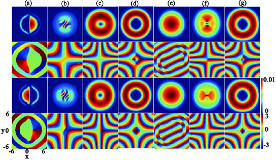
First focus on figure 1(a), i.e. the first column, where this is the situation that there is initial component separation and no applied gradient magnetic field. The first and third row show that the two components have immiscible combination density patterns with semicircle and crescent shapes, and rows two and four display a hidden vortex (clockwise rotation) Wen1 ; Mithun ; Wen2 in each component due to the presence of SOC and DDI. Once weak quadrupole field is included, e.g. $B=1.5$ as in column (b), the system exhibits an unusual, staggered stripe phase with a half-quantum vortex, where the two component densities are spatially separated from each other. The phase profiles show that there is a singly quantized hidden vortex in the spin-down component and both the phase profiles display quadrupole-like distribution JLi . We call it a quadrupole stripe phase with a half-quantum vortex to distinguish it from the conventional stripe phase in spin-orbit-coupled spin-$1/2$ BECs Zhai ; YZhang ; CWang ; XXu . When the quadrupole field strength increases to $B=4$, as in (c), the system displays obvious phase mixing with a singly quantized visible vortex in the spin-down component and a dark soliton in the spin-up component, as can be clearly seen in the figure. With the further increase of quadrupole field strength, the density distributions of the two components become almost the same with a large density hole in each component (figure 1(d)). Here the density hole is not an ordinary giant vortex but an exotic hidden vortex-antivortex cluster composed of several hidden vortices and antivortices (anticlockwise rotation), which is quite different from the previous cases of rotating BECs with or without SOC XXu ; Fetter ; XFZhou ; Aftalion .

For the case of initial phase mixing without the quadrupole filed, the ground state is a typical plane-wave phase (i.e.TF phase) as displayed in figure 1(e). When $B=1.5$, a singly quantized antivortex forms in the spin-up component while the density of the spin-down component keeps a TF distribution with the phase profile exhibiting quadrupole-like distribution (figure 1(f)). We call it quadrupole TF phase with a half-quantum antivortex to distinguish from the usual plane-wave phase. As the quadrupole field strength increases to $B=5$ (figure 1(g)), the densities of the two components are almost completely mixed with different hidden vortex-antivortex clusters being generated in the central regions, which is similar to that in figure 1(d).

III.2 Role of SOC

Next we consider the effects of SOC on the density and phase distributions of the ground states of spin-orbit-coupled BECs, now with fixed DDI and fixed in-plane gradient magnetic field, where the distributions are shown in figure 2. The gradient magnetic field is $B=2.5$, the dipolar coupling is $\gamma_{dd}=0.5$, and the intra- and interspecies interaction strengths are $\beta_{11}=\beta_{22}=800$, with $\beta_{12}=1600$ for the left three columns and $\beta_{12}=600$ for the right three columns. The rows from top to bottom represent $\left|\psi_{1}\right|^{2}$, arg$\psi_{1}$, $\left|\psi_{2}\right|^{2}$, and arg$\psi_{2}$, just as before. The changing SOC strengths are $\lambda_{x}=\lambda_{y}=0$ (a), $\lambda_{x}=\lambda_{y}=3$ (b), $\lambda_{x}=\lambda_{y}=5$ (c), $\lambda_{x}=\lambda_{y}=1$ (d), $\lambda_{x}=\lambda_{y}=5$ (e), and $\lambda_{x}=\lambda_{y}=10$ (f).

Figure 2: (Color online) Ground-state density distributions and phase distributions for spin-orbit-coupled dipolar BECs in a harmonic trap and an in-plane quadrupole field. The rows from top to bottom denote $\left|\psi_{1}\right|^{2}$, arg$\psi_{1}$, $\left|\psi_{2}\right|^{2}$, and arg$\psi_{2}$. The parameters are $B=2.5$, $\gamma_{dd}=0.5$, $\beta_{11}=\beta_{22}=800$, $\beta_{12}=1600$ (left three columns), and $\beta_{12}=600$ (right three columns). (a) $\lambda_{x}=\lambda_{y}=0$, (b) $\lambda_{x}=\lambda_{y}=3$, (c) $\lambda_{x}=\lambda_{y}=5$, (d) $\lambda_{x}=\lambda_{y}=1$, (e) $\lambda_{x}=\lambda_{y}=5$, and (f) $\lambda_{x}=\lambda_{y}=10$. The unit length is $a_{0}$.

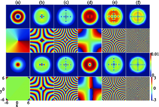
For the case of initial component separation, when there is no SOC (i.e. $\lambda_{x}=\lambda_{y}=0$), the topological structure of the system is a typical Anderson-Toulouse coreless antivortex Anderson , where the core of the circulating external component is filled with the other nonrotating component (see figure 2(a)). With the increase of SOC strength, the system favors an exotic topological structure consisting of two criss-crossed vortex and antivortex strings as shown in figures 2(b) and 2(c), where the vortex string is distributed along the $x$ direction while the antivortex string is distributed along the $y$ direction. Although there are vortex-antivortex clusters or vortex-antivortex strings in individual components, there is no phase defect in the total density distribution of the system. It is indicated that the topological quantum states are novel Anderson-Toulouse coreless vortex-antivortex cluster (string) states, and have not been observed in previous studies. The vortices and antivortices in different components repel each other and distribute staggeredly at different positions due to the repulsion between the vortices or the antivortices. For the case of initial component mixing and weak SOC, e.g. $\lambda_{x}=\lambda_{y}=1$, the ground state of the system is a half-quantum vortex state with only a singly quantized vortex being generated in the spin-down component (see figure 2(d)), which is somewhat similar to that in figure 2(a). For strong SOC, the criss-crossed vortex-antivortex string structures become noticeable (see figures 2(e) and 2(f)), which is similar to the case of initial phase separation and large SOC strength.

What is happening physically is the spin-orbit interaction induces the coupling between the atomic spin and the center-of-mass motion of the BEC. Thus varying the SOC strength will lead to the change of the atomic spin structure as well as the spin texture of the system. From figures 2(b), 2(c), 2(e) and 2(f), the vortex (antivortex) number in each component evidently increases because the stronger SOC means there is a larger orbital angular momentum input into the system, regardless of the initial state of the system being mixed or separated. On the other hand, the interplay among SOC, DDI and in-plane gradient magnetic field will change the symmetry of vortex distribution in the system. As a result, for strong SOC, the criss-crossed vortex-antivortex string, rather than a conventional triangular vortex lattice, dominates the topological structure of the system.

III.3 Role of DDI

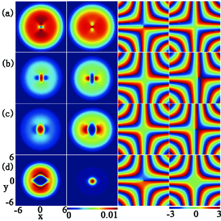
The next stage is to consider the effect of DDI on the ground-state structure of initially immiscible BECs with fixed SOC and gradient magnetic field. As mentioned before, we consider that the dipolar atoms are polarized along the condensate plane, i.e. $\alpha=\pi/2$. Figure 3 shows the density distributions and phase distributions for the ground states of the system, where $\beta_{11}=\beta_{22}=800$, $\beta_{12}=1600$, $\lambda_{x}=\lambda_{y}=2$, and $B=1.5$.

Considering figure 3(a), in the absence of DDI ($\gamma_{dd}=0$), there is an antivortex in the spin-up component and the phase distributions of the two components exhibit quadrupole-like profile, which indicates the ground state of the system is a coreless half-quantum antivortex state with quadrupole phase distribution. This feature evidently originates from the combination of the effects of SOC and the in-plane gradient magnetic field because previous studies show that the system of two-component BECs with only SOC only supports two typical quantum phases: a plane-wave phase and a stripe phase. In the presence of relatively weak DDI, e.g. $\gamma_{dd}=0.5$ and $\gamma_{dd}=0.7$, the system forms a sandwich-like structure, with the two component densities being spatially separated in the central regions, and a vortex is created in the center of the spin-down component (see figures 3(b) and 3(c)).

For strong DDI, i.e. when $\gamma_{dd}=1$, the system sustains a particular delaminated structure with a quadrupole phase profile in both components. This means the density distributions of the two components are separated fully and a prolate antivortex along the $x$ direction is generated in the spin-up component (figure 3(d)). When DDI increases further and exceeds a critical value, such as $\gamma_{dd}=1.2$, the system collapses and the BECs disappear. This is due to the strong effective attraction caused by the DDI. For the case of initial phase mixing, our simulation shows that the ground-state structures are similar to those in the case of initial phase separation, so there is no need to show them.

Figure 3: (Color online) Density distributions and phase distributions for the ground states of dipolar BECs with SOC in a harmonic trap and an in-plane gradient magnetic field, where $\lambda_{x}=\lambda_{y}=2$, $B=1.5$, $\beta_{11}=\beta_{22}=800$, and $\beta_{12}=1600$. The columns from left to right denote $\left|\psi_{1}\right|^{2}$, $\left|\psi_{2}\right|^{2}$, arg$\psi_{1}$, and arg$\psi_{2}$. These plots are for different strengths of DDI, with (a) $\gamma_{dd}=0$, (b) $\gamma_{dd}=0.5$, (c) $\gamma_{dd}=0.7$, and (d) $\gamma_{dd}=1$. The unit length is $a_{0}$.

To summarize the ground state structures we present table 1 where we briefly summarize the ground-state phases and the relevant critical values of driving parameters for different phases while maintaining $\beta_{11}\beta_{22}<\beta_{12}^{2}$. For fixed SOC and DDI with changing in-plane quadrupole field, as shown in figure 1, the system sustains semicircle and crescent phase with hidden vortices, quadrupole stripe phase with a half-quantum vortex, mixing phase with a half-quantum vortex and a dark soliton, and miscible phase with hidden vortex-antivortex cluster, depending on the quadrupole field strength. For fixed DDI and quadrupole field, with the increase of SOC strength, one can observe the Anderson-Toulouse coreless antivortex state and the criss-crossed vortex-antivortex cluster (or string) state. Lastly we investigated the effect of changing DDI in the presence of fixed SOC and gradient magnetic field, as shown in figure 3, and we find that the system can exhibit a coreless half-quantum antivortex state with quadrupole phase profile, a sandwich structure with a half-quantum vortex, or delaminated structure with a half-quantum antivortex.

Table 1: Combined effects of SOC, DDI and quadrupole field on ground state for $\beta_{11}\beta_{22}<\beta_{12}^{2}$

SOC	DDI	Quadrupole field	Ground state
$\lambda_{x}=\lambda_{y}=2$	$\gamma_{dd}=0.5$	$B\leqslant 0.5$	Semicircle and crescent phase with respective hidden vortices
$\lambda_{x}=\lambda_{y}=2$	$\gamma_{dd}=0.5$	$0.5<B<1.8$	Quadrupole stripe phase with a half-quantum vortex
$\lambda_{x}=\lambda_{y}=2$	$\gamma_{dd}=0.5$	$1.8\leqslant B<4.2$	Miscible phase with a half-quantum vortex and a dark soliton
$\lambda_{x}=\lambda_{y}=2$	$\gamma_{dd}=0.5$	$B\geqslant 4.2$	Miscible phase with hidden vortex-antivortex cluster
$\lambda_{x}=\lambda_{y}<2.6$	$\gamma_{dd}=0.5$	$B=2.5$	Anderson-Toulouse coreless antivortex
$\lambda_{x}=\lambda_{y}\geqslant 2.6$	$\gamma_{dd}=0.5$	$B=2.5$	Criss-crossed vortex-antivortex cluster (or string) state
$\lambda_{x}=\lambda_{y}=2$	$0\leqslant\gamma_{dd}<0.3$	$B=1.5$	Coreless half-quantum antivortex state with quadrupole phase profile
$\lambda_{x}=\lambda_{y}=2$	$0.3\leqslant\gamma_{dd}<0.9$	$B=1.5$	Sandwich structure with a half-quantum vortex
$\lambda_{x}=\lambda_{y}=2$	$0.9\leqslant\gamma_{dd}<1.2$	$B=1.5$	Delaminated structure with a half-quantum antivortex
$\lambda_{x}=\lambda_{y}=2$	$\gamma_{dd}\geqslant 1.2$	$B=1.5$	System collapses

III.4 Spin textures

Now we analyze the spin densities and spin textures of the system in order to further elucidate the ground-state properties. To consider this one looks at figure 4, which show the representative spin-density distributions (the top three rows) and the corresponding topological charge densities (the bottom row). The relevant parameters for the four cases are: (a) $\beta_{11}=\beta_{22}=800$, $\beta_{12}=1600$, $\lambda_{x}=\lambda_{y}=2$, $\gamma_{dd}=0.5$, $B=6$; (b) $\beta_{11}=\beta_{22}=800$, $\beta_{12}=1600$, $\lambda_{x}=\lambda_{y}=3$, $\gamma_{dd}=0.5$, $B=2.5$; (c) $\beta_{11}=\beta_{22}=800$, $\beta_{12}=600$, $\lambda_{x}=\lambda_{y}=5$, $\gamma_{dd}=0.5$, $B=2.5$ and (d) $\beta_{11}=\beta_{22}=800$, $\beta_{12}=1600$, $\lambda_{x}=\lambda_{y}=2$, $\gamma_{dd}=1$, $B=1.5$. The density distributions and phase distributions corresponding to figures 4(a)-4(d) are given in figure 1(d), figure 2(b), figure 2(e), and figure 3(d), respectively. In the pseudo-spin representation, the red region denotes spin-up and the blue region denotes spin-down. From figure 4, $S_{x}$ obeys an odd-parity distribution along the $x$ direction and an even-parity distribution along the $y$ direction, while the situation is the reverse for $S_{y}$. At the same time, $S_{z}$ and $q(r)$ satisfy an even-parity distribution along both the $x$ direction and the $y$ direction.

Figure 4: (Color online) Spin densities and topological charge densities of spin-orbit-coupled dipolar BECs in a harmonic trap and an in-plane quadrupole field. (a) $\beta_{11}=\beta_{22}=800$, $\beta_{12}=1600$, $\lambda_{x}=\lambda_{y}=2$, $\gamma_{dd}=0.5$, $B=6$, (b) $\beta_{11}=\beta_{22}=800$, $\beta_{12}=1600$, $\lambda_{x}=\lambda_{y}=3$, $\gamma_{dd}=0.5$, $B=2.5$, (c) $\beta_{11}=\beta_{22}=800$, $\beta_{12}=600$, $\lambda_{x}=\lambda_{y}=5$, $\gamma_{dd}=0.5$, $B=2.5$, and (d) $\beta_{11}=\beta_{22}=800$, $\beta_{12}=1600$, $\lambda_{x}=\lambda_{y}=2$, $\gamma_{dd}=1$, $B=1.5$. The rows (from top to bottom) denote $S_{x}$, $S_{y}$ and $S_{z}$ components of the spin density vector, and the topological charge density $q(r)$. The density distributions and phase distributions corresponding to (a)-(d) are given in Fig. 1(d), Fig. 2(b), Fig. 2(e), and Fig. 3(d), respectively. The unit length is $a_{0}$.

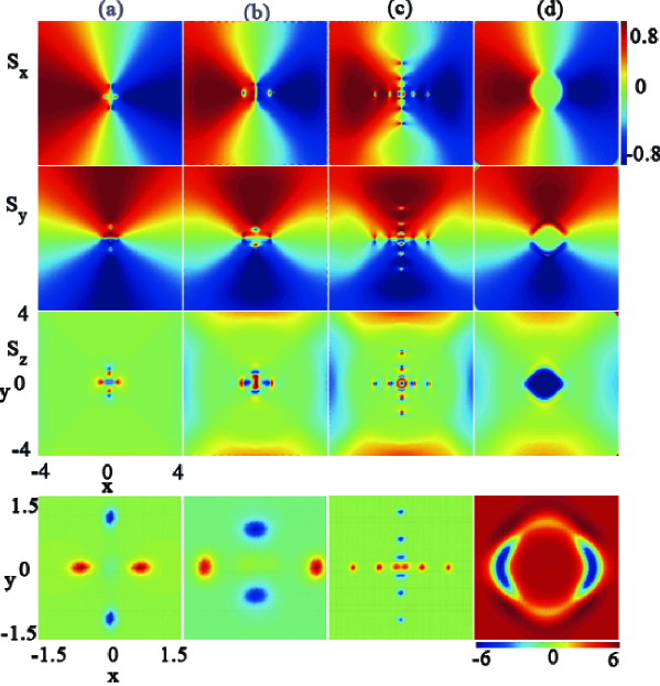
In addition, there are criss-cross crystal-like structures in the $S_{x}$, $S_{y}$, $S_{z}$ components of the spin density and the topological charge density $q(r)$ (see figures 4(a)-4(c)), which indicates that there exist special spin defects in the present system. Furthermore, two remarkable spin domains are generated in spin components $S_{x}$ and $S_{y}$, and the boundary between the two spin domains forms a peculiar hyperbolic spin domain wall with $\left|S_{x}\right|\neq 1$ and $\left|S_{y}\right|\neq 1$ due to the presence of in-plane quadrupole filed, which can be seen clearly in the top two rows of figure 4. It is well known that the spin domain wall for a system consisting of two-component BECs is typically a classical Neel wall, where the spin flips only along the perpendicular direction of the wall. However, our simulation shows that in the region of the domain wall the spin flips not only along the vertical direction of domain wall, but also along the domain-wall direction, which indicates that the observed hyperbolic domain wall is a new type of domain wall.

In figure 5, we give the spin textures of the system, where the parameters for the four rows are the same with those for figures 4(a)-4(d). Shown in the right three columns are the local enlargements of the spin textures in the left first column, so one can better see the details of the spin textures. Our simulation shows that the spin textures in figure 5 exhibit strong symmetry with respect to the $y=0$ axis and the $x=0$ axis, where the texture singularities are symmetrically distributed along the two axes. The excellent symmetry is also reflected in the topological charge densities in the bottom row of figure 4. In the context of this work, one only needs to focus on the left region, the upper region and the central region of the spin texture, as shown in columns 2-4 (from left to right) of figure 5. Our numerical calculation shows that the local topological charges in figures 5(a2), 5(a3) and 5(a4) approach $Q=1$, $Q=-1$, and $Q=-0.5$, respectively, which indicates the local topological defects in figures 5(a2), 5(a3) and 5(a4) are hyperbolic-radial(out) skyrmion, hyperbolic-radial(in) antiskyrmion, and hyperbolic half-antiskyrmion (antimeron) Su ; Shi ; CLiu ; Mermin , respectively. Thus the texture in figure 5(a1) forms a special skyrmion-half-antiskyrmion-antiskyrmion lattice composed of two hyperbolic-radial(out) skyrmions along the $x$ direction, two hyperbolic-radial(in) skyrmions along the $y$ direction, and a hyperbolic half-antiskyrmion in the center.

Figure 5: (Color online) Spin textures of dipolar BECs with SOC in a harmonic trap and an in-plane quadrupole field, where the corresponding spin densities and topological charge densities are given in Fig. 4. The parameters in the four rows from top to bottom are the same with those in Figs. 4(a)-4(d), respectively. Shown in left column 1 are the spin textures for various parameter values, and displayed in the right three columns are the local enlargements of the spin textures in the left first column. The unit length is $a_{0}$.

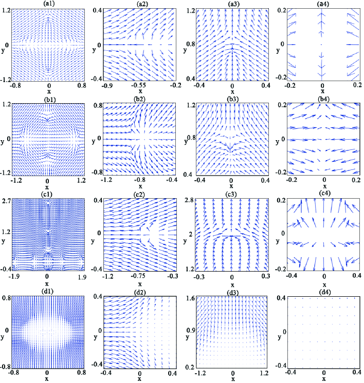
Though the component density distributions for the ground state in figure 2(b) are quite different from those in figure 1(d), the spin texture in figure 5(b1) is somewhat similar to that in figure 5(a1) and also posses strong symmetry. The local topological charge for the left spin defect (see figure 5(b2)) and the right spin defect is $Q=1$; and that for the upper spin defect (see figure 5(b3)) and the lower spin defect is $Q=-1$. The difference is that the local topological charge of the central spin defect (see figure 5(b4)) is $Q=0.5$. That is, the topological structure in figure 5(b1) is a skyrmion-half-skyrmion-antiskyrmion lattice made of hyperbolic-radial(out) skyrmions, hyperbolic-radial(in) skyrmions and a hyperbolic half-skyrmion (meron).

The spin texture for the ground state shown in figure 2(e) is richer and more interesting, which has SOC, DDI, quadrupole field and there is initial component mixing. Considering figure 5(c1), we see that it has good symmetry but also posses complexity in the spin texture. For the convenience of analysis, we mainly show the region of $y>0$ of the spin texture, where the representative local enlargements are displayed in figures 5(c2)-5(c4). Our calculation results show that the topological charge for individual spin defects (except for the central spin defect) along the $x$ the $y$ axes are $Q=0.5$ and $Q=-0.5$, respectively. This implies that the horizontal topological defects (except for the central defect) are hyperbolic half-skyrmions (merons) (see figure 5(c2)) and the vertical ones (except for the central defect) are hyperbolic half-antiskyrmions (antimerons) (see figure 5(c3)). The central topological defect is a radial-out skyrmion with local topological charge $Q=1$ (see figure 5(c4)). Therefore the topological structure in figure 5(c1) is an exotic half-skyrmion-skyrmion-half-antiskyrmion lattice composed of four horizontal half-skyrmions, one central skyrmion and six vertical half-antiskyrmions. Displayed in figure 5(d1) is a half-antiskyrmion (antimeron) with topological charge $Q=-0.5$. Compared with conventional half-skyrmion, there exists a large singularity region with a waist-drum shape in the spin texture (see figures 5(d1)-5(d4)), which is essentially caused by the presence of in-plane quadrupole field and strong DDI. To the best of our knowledge, these new topological structures mentioned above have not been reported in previous studies, and can be observed in future experiments.

IV Conclusion

We have studied a rich variety of ground-state phases and topological defects of quasi-2D two-component dipolar BECs with Rashba SOC in a harmonic trap and an in-plane gradient magnetic field. The combined effects of the in-plane gradient magnetic field, SOC, DDI, and interatomic interactions on the ground-state structure of this system were discussed systematically. Our results show that for strong quadrupole field and fixed SOC and DDI strengths the system favors a ring mixed phase with a hidden vortex-antivortex lattice (cluster) rather than a usual giant vortex in each component. In particular, for the case of initial component separation and relatively weak quadrupole field, the ground state is an unusual quadrupole stripe phase with a half-quantum vortex or a quadrupole TF phase with a half-quantum antivortex. For given DDI and quadrupole field strengths, increasing SOC strength leads to the formation of a criss-crossed vortex-antivortex string state. When the strengths of SOC and quadrupole field are fixed, the ground state for strong DDI exhibits a sandwich-like structure, or a special delaminated structure with a prolate antivortex in the spin-up component and quadrupole phase distribution in both components. The results for different parameter regimes can be easily seen in table 1. Furthermore, the typical spin textures of the system were analyzed. We find that the system supports exotic new topological defects, such as a hyperbolic spin domain wall, skyrmion-half-antiskyrmion(or half–skyrmion)-antiskyrmion lattice, half-skyrmion-skyrmion-half-antiskyrmion lattice, and drum-shaped half-antiskyrmion (antimeron). This work has numerically demonstrated the many complex, novel and interesting topological structures that are present in this system, and since it is expected that these results are to be verified in future experiments, this paper could serve as a valuable resource for experimentalists working on these systems and comparing theory and experiment. These findings have enriched our new understanding for topological excitations in ultracold atomic gases and condensed matter physics.