Spectral index$-$mass accretion rate correlation and evaluation of black hole masses in AGNs 3C 454.3 and M87

We present the discovery of correlations between the X-ray spectral (photon) index and mass accretion rate observed in active galactic nuclei (AGNs) 3C 454.3 and M87. We analyzed spectral transition episodes observed in these AGNs using Chandra, Swift, Suzaku, $Beppo$SAX, ASCA and RXTE data. We applied a scaling technique for a black hole (BH) mass evaluation which uses a correlation between the photon index and normalization of the seed (disk) component which is proportional to a mass accretion rate. We developed an analytical model that shows that the photon index of the BH emergent spectrum undergoes an evolution from lower to higher values depending on disk mass accretion rate. To estimate a BH mass in 3C 454.3 we consider extra-galactic SMBHs NGC 4051 and NGC 7469 as well as Galactic BHs Cygnus X–1 and GRO J1550–564 as reference sources for which distances, inclination angles are known and the BH masses are already evaluated. For M87 on the other hand, we provide the BH mass scaling using extra-galactic sources (IMBHs: ESO 243–49 HLX–1 and M 101 ULX–1) and Galactic sources (stellar mass BHs: XTE J1550–564, 4U 1630–472, GRS 1915+105 and H 1743–322) as reference sources. Application of the scaling technique for the photon index$-$mass accretion rate correlation provides estimates of the BH masses in 3C 454.3 and M87 to be about $3.4\times 10^{9}$ and $5.6\times 10^{7}$ solar masses, respectively. We also compared our scaling BH mass estimates with a recent BH mass estimate of $M_{87}=6.5\times 10^{9}M_{\odot}$ made using the Event Horizon Telescope which gives an image at 1.3 mm and is based on the angular size of the ‘BH event horizon’. Our BH mass estimate in M87 is at least two orders of magnitude lower than that made by the EHT team.

1 Introduction

Active galactic nuclei (AGNs) are ideal laboratories for studying the properties of matter in critical conditions. Especially interesting are radio-loud AGNs such as blazars and FR-I radio sources, which more often enter into active states and are accompanied by jet ejection events. Usually they are sources of multiwavelength radiation. It is also assumed that their energy is controlled by a supermassive black hole (BH) at their center.

Blazars constitute a sub-class of radio-loud AGNs characterized by broadband nonthermal emission from radio to $\gamma$-rays. It is generally proposed that bipolar relativistic jets closely align to our line of sight. They exhibit rapid variability and a high degree of polarization. Blazars with only weak or entirely absent emission lines in the optical band are historically classified as BL Lacertae objects, while others are classified as flat-spectrum radio quasars (FSRQs, see Urry & Padovani 1995).

Among the FSRQ class of blazars, 3C 454.3 (PKS 2251+158) is one of the brightest and most variable sources. This source is a well-known AGN and demonstrates significant variability in all energy bands (Unwin et al. 1997): optical (Villata et al. 2009; Raiteri et al. 1998, 2011), radio (Vol’vach et al. 2008, 2010, 2011, 2013, 2017), X–rays (Raiteri et al. 2011; Abdo et al. 2010), and $\gamma$-rays (Bonning et al. 2009; Abdo et al. 2009).

In the optical range, the blazar 3C 454.3 shows a change of active states. For example, in 2006–2007 the source remained in a faint state (Raiteri et al. 2007). Then, from July 2007 the source began an active phase, which was detected several times in $\gamma$-rays by the AGILE satellite. The source was monitored from the optical to the radio bands by the Whole Earth Blazar Telescope (WEBT) and its GLAST-AGILE Support Program (GASP, Villata et al. 2008). Vercellone et al. (2008), Raiteri et al. (2008a,b), Vercellone et al. (2009), Donnarumma et al. (2009), Villata et al. (2009), and Vercellone et al. (2010) published the results of these observations. GASP-WEBT (Global Aviation Safety Plan-Whole Earth Blazar Telescope) observations in 2009–2010 were performed in a number of observatories: Abastumani, Calar Alto data were acquired as part of the MAPCAT project, Crimean, Galaxy View, Goddard (GRT- Gamma Ray Telescope), Kitt Peak [(MDM), Michigan-Dartmouth-MIT Observatory] , Lowell (Perkins-Lowell Observatory), Lulin, New Mexico Skies, Roque de los Muchachos (KVA-Kungliga Vetenskapsacademien), Sabadell, San Pedro Martir, St. Petersburg, Talmassons, Teide (BRT-the Bradford Robotic Telescope ), Tijarafe, and Valle d’Aosta. Optical observations were also carried out by the UVOT instrument onboard the $Swift$ satellite (Raiteri et al. 2011). This optical object with a magnitude of $V=16.1^{m}$ was also identified as a radio source and classified as a highly polarized quasar with a redshift of $z=0.859$ (Jackson & Browne 1991).

A multi-wavelength study of the flaring behavior of 3C 454.3 during 2005–2008 was carried out by Jorstad et al. (2010). These latter authors discussed the activity of this object in terms of a core-jet with a knot structure and suggested that the emergence of a superluminal knot from the core relates to a series of optical and high-energy outbursts and that the millimeter-wave core lies at the end of the jet acceleration and collimation zone.

$Suzaku$ observations of 3C 454.3 in November 2008 analyzed by Abdo et al. (2010) confirmed the earlier suggestions by Raiteri et al. (2007, 2008b) that there is a soft X-ray excess, which becomes stronger when the $\gamma-$ radiation in this source gets fainter. These authors interpret this excess as either a contribution of the high-energy tail of the synchrotron component or bulk-Compton radiation produced as a result of Comptonization of the disk UV photons due to the relativistic jet plasma.

Despite the 3C 454.3 study based on multi-wave observations, the question of the mass of the central engine in 3C 454.3 still remains open. On the other hand, there is a problem with its extended structures, which are clearly visible on the radio images. We should also emphasize its strong variability which can be interpreted in the framework of the binary system model (see Volvach et al., 2017 and references there).

The mass of the super-massive black hole (SMBH) centered in 3C 454.3 is estimated to be within a the range of $M=(0.5-1.5)\times 10^{9}$ M_⊙ (Woo & Urry 2002; Liu et al. 2006; Sbarrato et al. 2012). Gu et al. (2001) concluded that the quasar contains a binary system of BHs with masses of $0.5-4\times 10^{9}M_{\odot}$, and Eddington luminosity that ranges from $6\times 10^{46}$ to $5\times 10^{47}$ erg/s (Khangulyan et al. 2013). The flow velocity of the relativistic jet probably ranges between $0.97c$ and $0.999c$ (Jorstad et al. 2005; Hovatta et al. 2009; Raiteri et al. 2011) and the angle to our line of sight is between 1^∘ and 6^∘ (Raiteri et al. 2011; Zamaninasab et al. 2013). Gupta et al. (2017) using optical data from the Steward observatory produced a more precise estimate of the BH mass of the central source using the broad Mg II line width and the continuum luminosity at 3000 Å: $M_{BH}=2.3\pm 0.5\times 10^{9}$ M_⊙ (see also Vestergaard & Osmer 2009).

It is known that 3C 454.3 is an active source accompanied by jet ejection events that are associated with a sharp increase in radio emission. The jet is also detected in X-rays. It is important to note that the most prominent extragalactic X-ray jet is well observed in AGN M87 [$E0$-type (Hubble, 1926), FR-I class], where several bright components (blobs) of this one-sided jet can be separately observed. In particular, the blob HST–1 is located less than 1” from the nucleus of M87, and is the closest of its kind to that position. It is interesting that the HST–1 flux sometimes becomes significantly higher than that of a nucleus component. Therefore, it is also important to separate the jet emission from the radiation of the nucleus.

In this paper we present our analysis of available Chandra, $Swift$, $Suzaku$, ASCA, BeppoSAX and $RXTE$ observations of 3C 454.3 and M87 and also reexamine previous conclusions on the BH nature of these AGNs. Furthermore, we find further indications to supermassive BHs in 3C 454.3 and M87. In Sect. 2 we present the list of observations used in our data analysis, and in Sect. 3 we provide details of the X-ray spectral analysis. We discuss the evolution of the X-ray spectral properties during the spectral state transitions and present the results of the scaling analysis to estimate a BH mass for these AGNs in Sect. 4. We present our final conclusions on the results in Sect. 5.

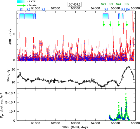
Figure 1: Evolution of ASM/RXTE count rate (2-12 keV, top), radio (8 GHz, middle) and $\gamma$-ray radiation (0.1–300 GeV, bottom) during 1996 – 2012 observations of 3C 454.3. Vertical arrows (at top of the panels) indicate temporal distribution of the RXTE (blue) and $Suzaku$ (green) data sets listed in Tables 1$-$7.

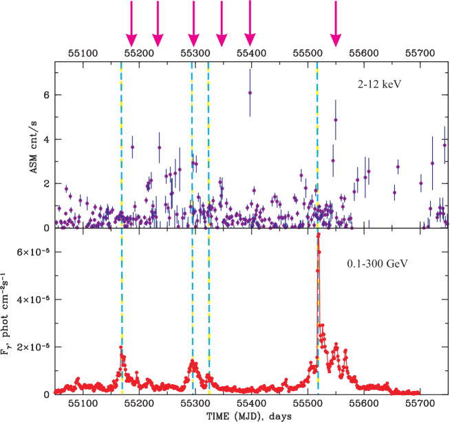
Figure 2: On delays of peak-fluxes for outburst of 3C 454.3 observed in 2010–2012 for two bands: 2–12 keV (top) and 0.1–300 GeV (bottom). Vertical $blue$ dashed lines mark the peak of $\gamma$-ray flux, while pink arrows (at top of the panels) indicate the peaks of X-ray bursts.

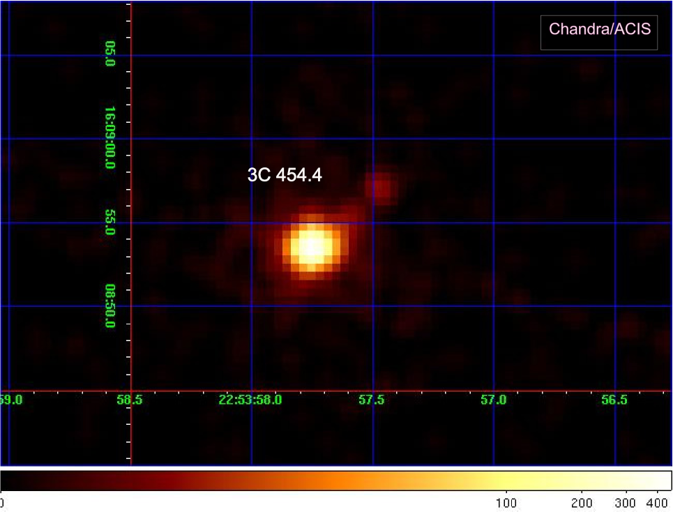
Figure 3: $Chandra$/ASIS (0.3$-$10 keV) image of 3C 454.3 field of view on November 6, 2002 with the exposure of 4929 s (MJD=52584).

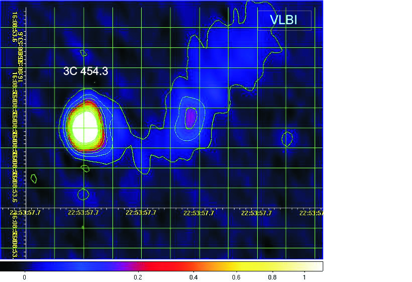
Figure 4: Adaptively smoothed $VLBI$ image of radio emission of 3C 454.3 field detected on March 10, 1997. Contours correspond to nine logarithmic intervals in the range of $3\times 10^{-3}-$5% with respect to the brightest pixel.

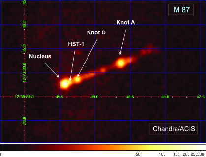
Figure 5: $Chandra$ X-ray images on April 14, 2017, with strong HST–1, with 5 ks exposure. We indicate the nucleus, the flaring knot HST-1 (0.86” from the nucleus), knot D, and knot A.

2 Observations and data reduction

Along with the long-term RXTE observations (1996–2010) described in Sect. 2.6, 3C 454.3 was also observed by $Suzaku$ (2007 – 2010, see Sect. 2.1), $Swift$ (2005–2010, see Sect. 2.4), and $Chandra$ (2002, 2004, see Sect. 2.5). On the other hand, M87 was observed by RXTE (1997 – 1998 and 2010), which is described in Sect. 2.6, $Beppo$SAX (1996; Sect. 2.3), $Chandra$ (1996; Sect. 2.5), $Suzaku$ (2006, see Sect. 2.1), and $ASCA$ (1993, see Sect. 2.2). We extracted these data from the HEASARC archives and found that they cover a wide range of X-ray luminosities for both sources. We should recognize that the well-exposed Suzaku data are preferable for the determination of low-energy photoelectric absorption. Therefore, we start our study using $Suzaku$ data of 3C 454.3. We also apply up-to-date SMART optical/near-infrared light curves that are available at www.astro.yale.edu/smarts/glast/home.php.

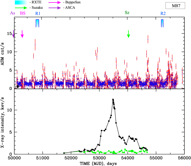
Figure 6: Top: Evolution of ASM/RXTE count rate during 1996 – 2012 observations of M87. Vertical arrows (at the top of panel) indicate temporal distribution of the RXTE (blue) and $Suzaku$ (green) data sets listed in Tables 1$-$7. Bottom: Evolution of $Chandra$ X-ray intensity of the nucleus (green) and HST-1 (black) during 2000 – 2008 observations of M87 according to data taken from Harris et al. (2009).

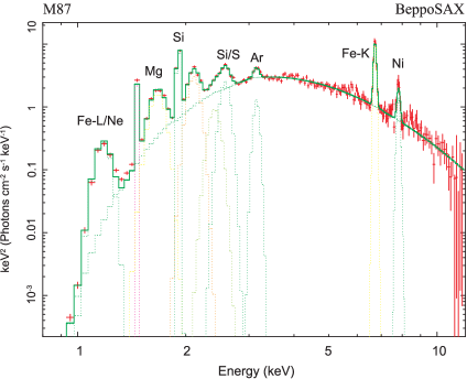
Figure 7: Best-fit BeppoSAX spectrum of M87 in the IS–HSS state (ID=60010001) using the tbabs*bmc+N*gauss model [$\chi^{2}_{red}=$ 1.05 (249 dof)]. The best-fit parameters are $\Gamma=$ 2.9$\pm$0.1 and $T_{s}=$ 140$\pm$10 eV. (see more detalis in Table 4). The data are denoted by red crosses, while the spectral model is presented by a green histogram.

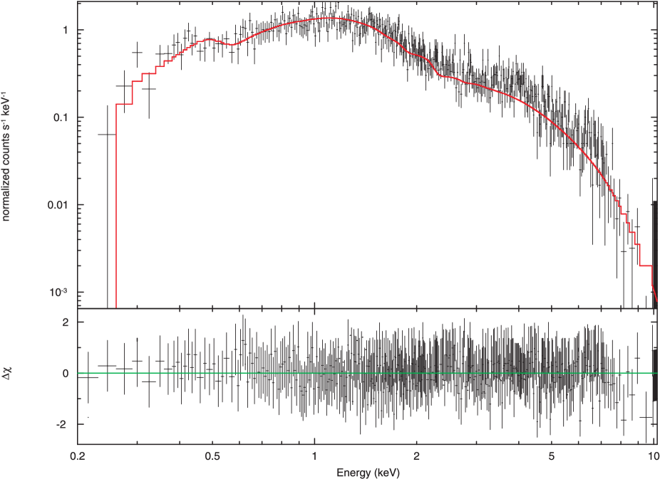
Figure 8: Best-fit Swift spectrum of 3C 454.3 for the IS using the tbabs*bmc model [$\chi^{2}_{red}=$ 1.02 (770 dof)]. The best-fit parameters are $\Gamma=$1.63$\pm$0.1 and $T_{s}=$280$\pm$20 eV. The data are denoted by black crosses, while the spectral model is presented by a red histogram.

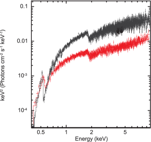
Figure 9: Two representative EF(E) spectral diagrams for the low/hard state (red, id=703006010) and for the intermediate state (black, id=904003010) of 3C 454.3 obtained with $Suzaku$.

Table 1: List of $Suzaku$ observations of 3C 454.3 and M87 used in our analysis

Object	Number of set	Obs. ID	Start time (UT)		End time (UT)	MJD interval
3C 454.3	Sz1	703006010	2008 Nov 22 09:18:32		2008 Nov 23 16:31:19	54792.4 – 54793.71
	Sz2	705021010	2010 Nov 25 01:11:14		2010 Nov 26 00:20:19	55525.2 – 55526.8
	Sz3	904003010	2009 Dec 9 02:40:43		2009 Dec 9 23:31:24	54439.2 – 54439.8
	Sz4	902002010	2007 Dec 5 04:57:55		2007 Dec 6 02:40:14	55174.1 – 55175.4
M87	Sz	801038010	2006 Nov 29 22:02:65		2006 Dec 2 03:02:24	54068.9 – 54071.1

Table 2: Best-fit parameters of the $Suzaku$ and $Chandra$ spectra of 3C 454.3 in the 0.3$-$10 keV range using the following five models^†: tbabs*power, tbabs*bbody, tbabs*(bbody+power), tbabs*bmc and tbabs*(bmc+power).

	Parameter	703006010	705021010	904003010	902002010	3127	4843
Model
tbabs	NH ($\times 10^{21}$ cm-2)	2.8$\pm$0.7	3.28$\pm$0.06	3.1$\pm$0.06	3.2$\pm$0.4	0.5$\pm$0.1	0.8$\pm$0.4
Power-law	$\Gamma_{pow}$	1.46$\pm$0.01	1.48$\pm$0.01	1.54$\pm$0.01	1.56$\pm$0.01	0.79$\pm$0.03	1.29$\pm$0.02
	N${}_{pow}^{\dagger\dagger}$	32.5$\pm$0.9	130$\pm$2	139$\pm$2	139.6$\pm$0.1	6.24$\pm$0.04	12.72$\pm$0.03
	$\chi_{red}^{2}$ (d.o.f.)	1.23 (1058)	1.24 (1797)	1.06 (1449)	2.00 (1643)	1.28 (282)	1.36 (441)
tbabs	NH ($\times 10^{21}$ cm-2)	0.09$\pm$0.01	0.08$\pm$0.03	0.06$\pm$0.01	0.08$\pm$0.2	0.03$\pm$0.01	0.01$\pm$0.01
Bbody	TBB (keV)	1.00$\pm$0.01	1.04$\pm$0.01	1.10$\pm$0.01	0.83$\pm$0.01	1.09$\pm$0.02	0.78$\pm$0.01
	N${}_{BB}^{\dagger\dagger}$	2.1$\pm$0.3	8.68$\pm$0.08	8.62$\pm$0.09	7.57$\pm$0.05	0.93$\pm$0.05	0.9$\pm$0.1
	$\chi_{red}^{2}$ (d.o.f.)	4.76 (1058)	13.2 (1797)	6.96 (1449)	13.08 (1643)	2.59 (282)	6.7 (441)
tbabs	NH ($\times 10^{21}$ cm-2)	5.5$\pm$0.2	5.4$\pm$0.1	5.3$\pm$0.4	5.8$\pm$0.6	0.85$\pm$0.02	0.9$\pm$0.3
Bbody	TBB (keV)	2.46$\pm$0.09	2.75$\pm$0.08	2.16$\pm$0.05	2.04$\pm$0.3	1.9$\pm$0.6	5.7$\pm$0.4
	N${}_{BB}^{\dagger\dagger}$	2.8$\pm$0.2	10.6$\pm$0.5	8.3$\pm$0.2	8.58$\pm$0.2	15$\pm$4	170$\pm$10
Power-law	$\Gamma_{pow}$	2.74$\pm$0.08	2.43$\pm$0.05	2.59$\pm$0.06	2.85$\pm$0.05	1.19$\pm$0.09	1.44$\pm$0.05
	N${}_{pow}^{\dagger\dagger}$	69$\pm$4	240$\pm$8	251$\pm$9	284$\pm$8	7.09$\pm$0.08	0.13$\pm$0.05
	$\chi_{red}^{2}$ (d.o.f.)	0.95 (1056)	0.93 (1795)	0.86 (1447)	0.86 (1641)	1.18 (280)	1.27 (439)
tbabs	NH ($\times 10^{21}$ cm-2)	5.6$\pm$0.2	7.4$\pm$0.5	3.0$\pm$0.2	3.9$\pm$0.2	5.8$\pm$0.2	5.0$\pm$0.1
bmc	$\Gamma_{bmc}$	1.51$\pm$0.03	2.01$\pm$0.09	1.99$\pm$0.02	1.98$\pm$0.01	1.11$\pm$0.03	1.24$\pm$0.02
	Ts (eV)	180$\pm$50	132$\pm$20	120$\pm$9	210$\pm$10	260$\pm$20	100$\pm$10
	$\log A$	-0.14$\pm$0.01	-0.35$\pm$0.01	-0.80$\pm$0.01	-0.41$\pm$0.04	2.†††	2.†††
	N${}_{bmc}^{\dagger\dagger}$	2.51$\pm$0.09	18.0$\pm$0.1	20.3$\pm$0.1	11.2$\pm$0.1	1.1$\pm$0.1	0.9$\pm$0.1
	$\chi_{red}^{2}$ (d.o.f.)	1.19 (1056)	1.06 (1795)	1.03 (1447)	1.02 (1641)	1.05 (279)	1.14 (438)
tbabs	NH ($\times 10^{21}$ cm-2)	5.6$\pm$0.2	7.4$\pm$0.5	3.0$\pm$0.2	3.9$\pm$0.2	0.2$\pm$0.1	1.2$\pm$0.1
bmc	$\Gamma_{bmc}$	1.51$\pm$0.03	2.01$\pm$0.09	1.99$\pm$0.02	1.98$\pm$0.01	1.12$\pm$0.02	1.36$\pm$0.06
	Ts (eV)	170$\pm$40	130$\pm$10	120$\pm$9	200$\pm$10	112$\pm$2	104$\pm$2
	$\log A$	-0.18$\pm$0.02	-0.37$\pm$0.04	-0.83$\pm$0.05	-0.42$\pm$0.08	0.22$\pm$0.09	0.42$\pm$0.06
	N${}_{bmc}^{\dagger\dagger}$	2.51$\pm$0.09	17$\pm$1	20.2$\pm$0.3	11.3$\pm$0.2	0.76$\pm$0.09	0.5$\pm$0.1
Power-law	$\Gamma_{pow}$	2.83$\pm$0.07	2.49$\pm$0.04	2.61$\pm$0.02	2.91$\pm$0.04	-2.5$\pm$0.3	-2.5$\pm$0.4
	N${}_{pow}^{\dagger\dagger}$	70$\pm$3	330$\pm$5	139$\pm$	98$\pm$5	0.01$\pm$0.01	0.01$\pm$0.01
	$\chi_{red}^{2}$ (d.o.f.)	10.08 (1054)	1.02 (1793)	1.00 (1445)	1.03 (1639)	1.09 (278)	1.2 (437)

Table 3: List of $ASCA$ and $Beppo$SAX observations of M87 used in our analysis

Satellite	Obs. ID	Start time (UT)		End time (UT)	MJD interval
$ASCA$	60033000	1993 Jun 7 19:15:48		1993 Jun 8 07:10:36	49145.8 – 49146.3
$Beppo$SAX	60010001	1996 Jul 14 21:31:00		1996 Jul 15 10:57:10	50278.8 – 50279.4

Table 4: Best-fit parameters of the $Beppo$SAX and $ASCA$ spectra of M87 in the 0.3$-$10 keV range^†. Errors are given at the 90% confidence level.

ID	$\alpha=$	$T_{s}$	$log(A)$	$N_{bmc}^{\dagger\dagger}$	$E_{cut}$	$E_{fold}$	$E_{Fe}$	$\sigma_{Fe}$	$N_{Fe}^{\dagger\dagger}$	$\chi_{red}$
	$\Gamma-1$	(eV)			(keV)	(keV)	(keV)	(keV)		(dof)
6001000	1.9$\pm$0.1	140$\pm$20	0.72$\pm$0.6	1.1$\pm$0.1	3.6$\pm$0.1	9.8$\pm$0.4	6.5$\pm$0.1	0.7$\pm$0.1	0.10$\pm$0.01	0.95 (40)
60033000	1.4$\pm$0.1	139$\pm$30	2.00†††	0.59$\pm$0.08	3.5$\pm$0.1	9.9$\pm$0.6	6.4$\pm$0.1	0.6$\pm$0.1	0.09$\pm$0.01	0.95 (40)

Table 5: List of $Swift$ observations of 3C 454.3 used in our analysis

Obs. ID	Start time (UT)		End time (UT)	MJD interval
00030024(001,002)	2005 May 11		2005 May 19	53501 – 53509
00031018(001,003-008)	2007 Nov 15		2007 Dec 15	54419 – 54449
00031216(001-011,013-016,018-027,029-044,046-063)	2008 May 27		2008 Oct 2	54613 – 54741
00031493(003,004)	2009 Sep 18		2009 Sep 19	55092 – 55093
00035030(001,003,005-010, 013-016,027-067)	2005 Apr 24		2009 Sep 16	53484 – 55090
00035030(113,114,175,178,180-189,190-193,195-204)	2010 Nov 3		2011 Jun 17	55503 – 55729
00090023(001-008)	2008 Sep 9		2009 Jun 1	54718 – 54983
00090081(001,002)	2009 Aug 13 12:56:32		2009 Sep 13 20:37:05	55056 – 55087

2.1 Suzaku data

$Suzaku$ observed 3C 454.5 throughout the time period from 2008 to 2010 and investigated M87 in 2006. Table 1 summarizes the start time, end time, and the MJD interval for each of these observations. One can see a description of the Suzaku experiment in Mitsuda et al. (2007). For observations obtained using a focal X-ray CCD camera (XIS, X-ray Imaging Spectrometer, Koyama et al. 2007), which is sensitive over the 0.3–12 keV range, we used software of the Suzaku data processing pipeline (ver. 2.2.11.22). We carried out the data reduction and analysis following the standard procedure using the latest HEASOFT software package (version 6.25) and following the Suzaku Data Reduction Guide. The spectra of the sources were extracted using spatial regions centered on the nominal positions of 3C 454.3 and M87 ($\alpha=22^{h}53^{m}57^{s}.77$, $\delta=+16^{\circ}08{\tt{}^{\prime}}53{\tt{}^{\prime\prime}}.6$, J2000.0 for 3C 454.3 and $\alpha=12^{h}30^{m}49^{s}.42$, $\delta=+12^{\circ}23{\tt{}^{\prime}}28{\tt{}^{\prime\prime}}.04$, J2000.0 for M87), while a background was extracted from source-free regions which have a comparable size away from the source. The spectrum data were re-binned to provide at least 20 counts per spectral bin to validate the use of the $\chi^{2}$-statistic. We carried out spectral fitting applying XSPEC v12.10.1. The energy ranges around 1.75 and 2.23 keV were not used for spectral fitting because of the known artificial structures in the XIS spectra around the Si and Au edges. Therefore, for spectral fits we chose the 0.3 – 10 keV range for the XISs (excluding 1.75 and 2.23 keV points).

The source count rate was variable by 40% for 3C 454.3 and 60% for M87. We fitted the spectral data using a number of models (see Sec. 3.2.1) but the best-fits are obtained using the XSPEC BMC model (see Titarchuk et al. 1997) modified by absorption by neutral gas of the solar composition (the XSPEC $tbabs$ model). Using this model we found that the amplitude of X-ray flux variability changed by up to a factor of two. The results of the fits are given in Table 2.

2.2 ASCA data

ASCA observed M87 on June 7–8, 1993. Table 3 summarizes the start time, end time, and the MJD interval for this observation. A description of the ASCA experiment can be found in Tanaka, Inoue, & Holt (1994). The solid imaging spectrometers (SIS) operated in Faint CCD-2 mode. The ASCA data were screened using the ftool ascascreen and the standard screening criteria. The spectrum for the source was extracted using spatial regions with a diameter of 3^′ (for SISs) and 4^′ (for GISs) centered on the nominal position of M87, while background was extracted from source-free regions of comparable size away from the source. The spectrum data were rebinned to provide at least 20 counts per spectral bin to validate the use of the $\chi^{2}$-statistic. The SIS and GIS data were fitted applying XSPEC in the energy ranges of 0.6 – 10 keV and 0.8 – 10 keV, where the spectral responses are best known.

2.3 BeppoSAX data

We used $Beppo$SAX data of M87 carried out on June 14–15, 1996. In Table 4 we show the log of the BeppoSAX observation analyzed in this paper. Generally, broadband energy spectra of M87 Lac were obtained combining data from three BeppoSAX narrow-field instruments (NFIs): the Low Energy Concentrator Spectrometer [LECS; Parmar et al. (1997)] for the 0.3 – 4 keV range, the Medium Energy Concentrator Spectrometer [MECS; Boella et al. (1997)] for the 1.8 – 10 keV range, and the Phoswich Detection System [PDS; Frontera et al. (1997)] for the 15 – 200 keV range. The SAXDAS data analysis package is used for the data processing. We performed a spectral analysis for each of the instruments in a corresponding energy range within which a response matrix is well specified. The LECS data have been renormalized to match the MECS data. Relative normalizations of the NFIs were treated as free parameters in the model fits, except for the MECS normalization that was fixed at unity. While the source is bright and background is low and stable, we checked its uniform distribution across the detectors. Furthermore, we extracted a light curve from a source-free region far from source and stated that background was not varying during the whole observation. Additionally, spectra were rebinned in accordance with the energy resolution of the instruments using rebinning template files in GRPPHA of XSPEC to obtain a better signal-to-noise ratio. Systematic uncertainties of 1% were applied to these analyzed spectra.

2.4 Swift data

We used the $Swift$ observation of 3C 454.3 and M87 carried out from 2005 to 2011 (Table 5). The Swift/XRT data were taken in Photon-Counting (PC) and Windowed Timing (WT) modes. The PC mode is characterized by high sensitivity but can be affected by the photon pile-up effect when the count rate is higher than $\sim$0.5 cts/s, while the WT mode does not suffer from a photon pile-up effect up to $\sim$200 cts/s. Data were processed using the HEASOFT v6.14, the tool XRTPIPELINE v0.12.84, and the calibration files (CALDB version 4.1). The ancillary response files were created using XRTMKARF v0.6.0 and exposure maps generated by XRTEXPOMAP v0.2.7. We selected source events for which the grades are accumulated in the range 0$-$12 and used default screening parameters to produce level 2 cleaned event files. To avoid photon pile-up effect during high-count-rate events, we extract the spectral data obtained in the PC mode in an annular region with inner and outer radii of 6 and 20 pixels, respectively (Vaughan et al. 2005). The background was estimated in a nearby source-free circular region of 50 pixels in radius. For the WT data mode we extracted spectra in a 40$\times$20 pixel rectangular region centered on the nominal position of 3C 454.3. The background was estimated in a nearby 50$\times$20 pixel source-free rectangular region. Spectra were re-binned to include at least 20 photons in each energy channel in order to use $\chi^{2}$-statistics. We fitted the spectrum using the response file SWXPC0TO12S6$\_$20010101v012.RMF. We also used the online XRT data product generator to obtain the image, light curves, and spectra (including background and ancillary response files; Evans et al. 2007, 2009).

Table 6: List of $Chandra$ observations of 3C 454.3 and M87

Object	Obs. ID	Start time (UT)	MJD	Exposure time (s)
3C 454.3	31271	2002-11-06 21:26:22	52584	4930
	48431	2004-10-29 05:01:50	53221	18261
M87	115142,3	2010-04-15 20:32:42	55301	4528
	187832,3	2016-04-20 08:32:11	55301	36114
	210752,3	2018-04-22 03:31:16	58230	9132

(1) Gupta et al. 2017; (2) Abeamowski et al. 2012; (3) Harris et al. 2009.

Table 7: List of RXTE observations of 3C 454.3 and M87

Object	Number of set	Dates, MJD	RXTE Proposal ID	Dates UT
3C 454.3	R1	50181–50358	103601	Apr 8 – Oct 29, 1996
	R2	50389–50802	203461	Nov 2, 1996 – Dec 20, 1997
	R3	50816–50986	302641	Jan 3 – Jun 22, 1998
	R4	54309–54636	931501	July 28, 2007 – June 19, 2008
	R5	55170–55182	941501	Dec 5 – Dec 17, 2009
	R6	55293–55297	951491	Apr 7 – Apr 11, 2010
M87	R${}^{m87}_{1}$	50812–50846	302162	Dec 30, 1997 – Feb 2, 1998
	R${}^{m87}_{2}$	55296–55301	951452	Apr 10 – Apr 15, 2010

(1) Rivers et al. 2013. (2) Jorstad et al. 2010.

Table 8: Best-fit parameters of the $Chandra$ spectra of M87 in the 0.3$-$10 keV range using the following four models^†: tbabs*power, tbabs*bbody, tbabs*(bbody+power) and tbabs*bmc.

	Parameter	11514	18783	21075
Model
tbabs	NH ($\times 10^{20}$ cm-2)	4.03$\pm$0.01	5.4$\pm$0.6	7.2$\pm$0.1
Power-law	$\Gamma_{pow}$	1.98$\pm$0.06	2.18$\pm$0.07	1.96$\pm$0.07
	N${}_{pow}^{\dagger\dagger}$	4.3$\pm$0.3	1.9$\pm$0.2	7.1$\pm$0.1
	$\chi_{red}^{2}$ (d.o.f.)	0.76 (113)	0.62 (174)	0.65 (176)
tbabs	NH ($\times 10^{20}$ cm-2)	0.09$\pm$0.01	0.08$\pm$0.03	0.06$\pm$0.01
Bbody	TBB (keV)	0.47$\pm$0.02	0.50$\pm$0.01	0.62$\pm$0.02
	N${}_{BB}^{\dagger\dagger}$	0.14$\pm$0.09	0.07$\pm$0.01	0.27$\pm$0.03
	$\chi_{red}^{2}$ (d.o.f.)	2.73 (113)	1.95 (174)	1.49 (176)
tbabs	NH ($\times 10^{20}$ cm-2)	3.9$\pm$0.6	3.3$\pm$0.1	3.9$\pm$0.6
Bbody	TBB (keV)	0.45$\pm$0.09	0.28$\pm$0.03	0.44$\pm$0.09
	N${}_{BB}^{\dagger\dagger}$	0.10$\pm$0.08	0.02$\pm$0.01	0.05$\pm$0.01
Power-law	$\Gamma_{pow}$	1.96$\pm$0.09	1.88$\pm$0.05	1.83$\pm$0.09
	N${}_{pow}^{\dagger\dagger}$	4.4$\pm$0.3	1.26$\pm$0.6	5.2$\pm$0.1
	$\chi_{red}^{2}$ (d.o.f.)	0.79 (111)	0.59 (172)	0.86 (174)
tbabs	NH ($\times 10^{20}$ cm-2)	1.0$\pm$0.1	7.4$\pm$0.5	1.0$\pm$0.2
bmc	$\Gamma_{bmc}$	1.94$\pm$0.07	2.83$\pm$0.09	2.09$\pm$0.07
	Ts (eV)	136$\pm$7	168$\pm$10	220$\pm$9
	$\log A$	1.08$\pm$0.02	-2.29$\pm$0.07	1.47$\pm$0.05
	N${}_{bmc}^{\dagger\dagger}$	0.10$\pm$0.04	0.50$\pm$0.04	0.17$\pm$0.05
	$\chi_{red}^{2}$ (d.o.f.)	0.87 (111)	1.01 (172)	0.96 (174)

2.5 Chandra data

The object 3C 454.3 was also observed by Chandra in 2002 and 2004, and M87 was extensively investigated by Chandra: here we apply observations of 2010, 2016, and 2018. The used log of Chandra observations is presented in Table 6. We extracted spectra from the ACIS-S detector via the standard pipeline CIAO v4.5 package and calibration database CALDB 2.27. In Figure 3 we demonstrate the Chandra/ASIS (0.3$-$10 keV) image of the 3C 454.3 field of view on November 6, 2002, with the exposure of 4929 s (MJD=52584). We also identified intervals of high background level to exclude all high-background events. The Chandra spectra were produced and modeled over the 0.3$-$7.0 keV energy range.

2.6 RXTE data

For our analysis, we also applied publicly available data of the RXTE (Bradt et al., 1993) from October 1996 to December 2009 (for 3C454.3) and from December 1997 to February 1998 as well as April 2010 (for M87). These data consist of 160 observations related to the different spectral states of the source. For data processing we utilized standard tasks of the LHEASOFT/FTOOLS 6.25 software package. Spectral analysis was implemented using PCA Standard 2 mode data, collected in the 3$-$22 keV range. The standard dead-time correction procedure has been applied to these data. The data are available through the GSFC public archive. We modeled the RXTE spectra using XSPEC astrophysical fitting software and implemented a systematic uncertainty of 0.5% to all analyzed spectra. In Table 7 we present a list of the groups of observations which covers the complete sample of the state evolution of the source. In Figure 1 we show an evolution of ASM/RXTE count rate (2-12 keV, top), radio (8 GHz, middle), and $\gamma$-ray radiation (0.1–300 GeV, bottom) during 1996 – 2012 observations of 3C 454.3. Vertical arrows (at top of the panels) indicate temporal distribution of the RXTE (blue) and $Suzaku$ (green) data sets listed in Tables 1$-$7.

2.7 FERMI/LAT data

Gamma-ray data observed with Fermi/LAT were obtained from MJD 54690 to 58446 . The gamma-ray source 1FGL2253.9+1608 was positionally identified with 3C 454.3 (Sasada et al., 2012). Each point on the $\gamma$-ray light curve (Fig. 2) corresponds to a daily averaged photon flux integrated over energies from 100 MeV to 300 GeV. This plot shows that there is no correlation between gamma and X-ray flashes in 3C 454.3 observed in 2010–2012 for two bands: 2–12 keV (top) and 0.1–300 GeV (bottom).

3 Results

3.1 Images and light curves of 3C 454.3 and M87

For a deep image analysis, we used the Chandra images with sub-arcsecond-resolution data quality provided by ACIS-S onboard Chandra. The Chandra/ACIS-S (0.2-8 keV) image obtained during observations of 3C 454.3 on November 6, 2002, (with exposure of 5 ks, ObsID=3127) is shown in Fig. 3. For each observation, we extracted the source spectrum from a circular region of 1.25" radius centered on the source position of 3C 454.3 [$\alpha=22^{h}53^{m}57^{s}.7$, $\delta=16^{\circ}08{\tt{}^{\prime}}53{\tt{}^{\prime\prime}}.6$, J2000.0 (see details in (Abdo et al., 2010)) and 0.75" radius circular region centered on the source position of M87 ($\alpha=12^{h}30^{m}49^{s}.4$, $\delta=12^{\circ}23{\tt{}^{\prime}}28{\tt{}^{\prime\prime}}$, J2000.0 (see details in Akiyama et al. (2019)). For comparison in Figure 4 we show an image of the same area around 3C 454.3 in the radio band (15 GHz, VLBA) at the time of our observations (see $R2$ and Kellermann et al., 1998). It can be seen that even during a radio outburst with jet ejection, we observe a point source in X-rays. $Swift$ data processing is described in our previous paper (Titarchuk & Seifina, 2016).

The Chandra (0.3 – 10 keV) image of the 3C 454.3 field of view is shown in Fig. 3. In the center we can see a bright point-like X-ray source, which is well matched with the optical one ($\alpha=23^{h}53^{m}57^{s}.77$, $\delta=+16^{\circ}08{\tt{}^{\prime}}52{\tt{}^{\prime\prime}}.7$, J2000.0). This image was obtained during observations of 3C 454.3 between May 11, 2005, and June 17, 2011 (with exposure time of 277 ks). Figure 3 also demonstrates a very weak signature of the X-ray jet-like (elongated) structure and the minimal contamination by other point sources and diffuse emission around 3C 454.3.

On the other hand the jet-like structure in M87 is strong and knotted. The knot, which is close to the nucleus of M87 (so called as HST–1), is variable. Figure 5 shows a $Chandra$ X-ray image on April 14, 2017, with the strong HST–1 for 5 ks exposure. Here, we indicate the nucleus, the flaring knot HST-1 (0.86” from the nucleus), knot D, and knot A.

Before proceeding to details of the spectral fitting we study the long-term behavior of 3C 454.3 and M87, particularly in its active phases. We discuss a long-term one-day average X-ray light curve of 3C 454.3 detected by the RXTE ASM over the total lifetime of the mission (1996 – 2012, Fig. 1). The bright-blue rectangles indicate the MJD intervals of RXTE observations used in our analysis. Vertical green arrows (top of the panel) indicate temporal distribution of the Suzaku data sets listed in Table 1. It is clear that 3C 454.3 became brighter, on average, in 2009 – 2010 ($R5$, $R6$) in a soft X-ray band (1–12 keV) than in the 1996 – 1997 period (see $R1$, $R2$). Blue points show the source signal and red line indicates its error bars. The ASM monitoring observations are distributed more densely over time (1996 – 2012) than those of $Suzaku$ (2007 – 2010, Abdo et al. 2010). However, it can be seen that the $Suzaku$ observations cover the time interval with increased X-ray count-rate events.

We also wish to bring attention to the synchronous light curves in radio (8 GHz, middle panel in Fig. 1) and $\gamma$-ray bands (0.1–300 GeV, bottom panel) during 1996 – 2012 observations of 3C 454.3. (green) It can be seen here that although the radio flash of 3C 454.3 (middle panel) correlates with the amplification of the $\gamma-$ray radiation (bottom panel) from the source, the X-ray light curve of 3C 454.3 (top panel) shows a more frequent irregular variability, which does not correlate with global outburst in the radio and gamma-ray ranges.

In Figure 6 we display the evolution of ASM/RXTE count rate during 1996 – 2012 observations of M87 (top). Vertical arrows (at the top) indicate temporal distribution of the RXTE (blue) and $Suzaku$ (green) data sets listed in Tables 1$-$7. We also demonstrate the evolution of the X-ray intensity of the nucleus (green) and HST-1 (black) seen by $Chandra$ during 2000 – 2008 observations of M87 according to data taken from Harris et al. (2009) in the lower panel.

Regarding an issue of possible correlation between flares in the X-ray and $\gamma$-ray ranges (delay/lead), we did not find any correlation for the data of 3C 454.3 observed in 2010–2012 (Fig. 2) for two bands: 2–12 keV (top) and 0.1–300 GeV (bottom). In Fig. 2 we mark the peak of $\gamma$-ray flux by vertical blue dashed lines, while pink arrows (at top of the panels) indicate the peaks of X-ray bursts. Obviously, there is no correlation between $\gamma$ and X-ray flashes. Our conclusion is somewhat different from the conclusions of Volvach et al. (2019), but we may have used a different set of data.

3.2 Spectral Analysis

We used different spectral models in order to test them using all available data of 3C 454.3 and M87. We want to establish evolution between the low/hard state (LHS) and the intermediate state (IS) using these spectral models. We investigate the Chandra, $Susaku$, $Swift$ and $RXTE$ spectra to test the following XSPEC spectral models: powerlaw, Bbody, BMC, and their possible combinations.

3.2.1 Choice of spectral model

As a first step, we present $Suzaku$ and $Chandra$ spectral data of 3C 454.3 in the 0.3 – 10 keV energy range. We establish that the thermal model (black body) fits the low-energy part well, while providing an excess emission for $E>$ 3 keV (e.g., for $Sz2$ and $Sz4$ spectrum, $\chi^{2}_{red}$=13.2 (1797 d.o.f.) and $\chi^{2}_{red}$=13.08 (1643), respectively, at the top part of Table 2). We find that the black body model indicates very low absorption (less than $0.9\times 10^{20}$ cm^-2) for all $Sz1-Sz4$ spectra, and moreover, that this model gives unacceptable fit quality, $\chi^{2},$ for all spectra of $Swift$ data. However, we should note that the tbabs*power-law model provides better fits than the thermal one. No Susaku data can be fitted well by a single-component model. Indeed, a simple power-law model produces a soft excess below 0.6 keV. These significant positive residuals at low energies, less than 1.3 keV, suggest the presence of additional emission components in the spectrum. Therefore, we also tested a model consisting of blackbody and power-law components. The model parameters of this combined model are $N_{H}=5\times 10^{21}$ cm^-2; $kT_{bb}=100-260$eV and $\Gamma=1.1-2$. (see more in Table 2). The best fits of the Suzaku spectra were found using of the Bulk Motion Comptonization model (BMC XSPEC model, Titarchuk et al. (1997)). We should emphasize that all $Suzaku$ best-fit results were obtained using the same model for all spectral states. Therefore, further we applied the BMC model modified by the interstellar absorption to all our $Swift$ and $RXTE$ observations of 3C 454.3.

A similar result concerning the choice of spectral model was obtained for M87 using the Chandra spectra of the M87 core (see Table 8). Therefore, further we applied the BMC model modified by the interstellar absorption to all our Beppo$SAX$, $Suzaku$, $ASCA$, $Swift$ and $RXTE$ observations of M87. In Figure 7 we show one EF(E) spectral diagram for the IS using the BeppoSAX data. Interestingly, we found many emission features in the $Beppo$SAX spectrum and fitted the spectrum with the tbabs * (bmc + N * Gauss) model. However, these features may be associated with a remote shell. In fact, $Beppo$SAX data come from a vast area that includes both the nucleus and the jet and from the external parts of the AGN. Moreover, the spectra obtained using $Chandra$ for a narrower region of the nucleus of M87 (¡0.85") no longer contain emission features (see Fig. 12).

The same conclusion was drawn for the XMM observations (Kennea et al., 2000). Therefore, we continued to work with the Chandra spectra in order to select a model for fitting the radiation of the nucleus of M87. We also proceeded with a powerlaw model; it fits the spectrum well, but the data are poorly matched by the $\chi$-square criterion ($\chi^{2}_{red}=0.62$ for 174 dof, ID=18783, see top of the Table 8). The thermal black body model also fits the spectrum well, however it poorly approximates the regions of 0.3–1 keV (possibly related to the underestimation of absorption) and the energy region above 7 keV ($\chi^{2}_{red}=1.5$ for 176 dof, ID=21075). In this case, taking absorption into account unnecessary. It is worth noting that the above models provide a soft excess below 0.3 keV. To eliminate this drawback, we used a combined model consisting of black body and power-law components. This latter model also fits the spectrum of the M87 nucleus well, but this combined model is more phenomenological than the physical one. Therefore, in the subsequent step, we used the generic BMC model. This model describes the spectra of the M87 nucleus well in all states (see bottom in the Table 8).

It is important to emphasize that the log-parabolic power-law models (Kardashev, 1962; Massaro et al., 2004a,b, 2006) were used for analysis of the blazar spectra. Indeed, the log-parabolic model is one of the simplest ways to describe curved spectra when these show mild and nearly symmetric curvature around the maximum, instead of a sharp high-energy cut-off like that of an exponential. As it is described by Massaro et al. (2006) the log-parabolic model law has only one more parameter than a simple power-law. For example, one can see it applying Eq. (3) of Massaro et al. (2004) who apply this formula for photon spectra. This appropriate formula is

$$F(E)=K(E/E_{1})^{-[a+b\lg(E/E_{1})]}.$$ (1)

in which the reference energy $E_{1}$ is fixed at 1 keV and thus the spectrum is determined only by three parameters $K$, $a$ and $b$ and the energy dependent photon index is

$$\Gamma(E)=a+b\lg(E/E_{1}).$$ (2)

However, it is easy to show that this log-parabolic model is approximated by a single power-law for large E and frozen pivotE. In fact, if the index of this simplified broken power-law and log-parabolic model is too large then it leads to very high residuals at low-energies. This is a well-known effect of this simplification. The log-parabolic model often uses a $N_{H}$ fixed at galactic values (Massaro et al., 2004), and for sources where the internal absorption is not relevant. In fact, this is one of the motivations for not using this model in the context of the present analysis.

There are several advantages to using the BMC model with respect to other common approaches applied to studies of X-ray spectra of accreting compact objects, including a broken power-law and the log-parabolic model. First, the BMC is by nature applicable to the general case where there is an energy gain through not only thermal Comptonization but also via dynamic (bulk) motion Comptonization (see Titarchuk et al. 1997; Laurent & Titarchuk 1999; Shaposhnikov & Titarchuk 2006, for details). Second, with respect to the log-parabolic model, the BMC spectral shape has an appropriate low-energy curvature, which is essential for a correct representation of the lower-energy part of the spectrum. Long-term experience with log-parabolic components shows that the model fit with this component is often inconsistent with the $N_{H}$ column values and produces an unphysical component “conspiracy” with the highecut part. Specifically, when a multiplicative component highecut is combined with the BMC, the cutoff energies $E_{cut}$ are in the expected range of 20–30 keV, while in a combination with the log-parabolic, $E_{cut}$ often goes below 10 keV, resulting in unreasonably low values of the photon index. Furthermore, implementation of the log-parabolic model makes it much harder or even impossible to correctly identify the spectral state of the source, which is an imminent task for our study. An even more important property of the BMC model is that it consistently calculate

3.3 Spectral Analysis

We used different spectral models in order to test them using all available data of 3C 454.3 and M87. We want to establish evolution between the low/hard state (LHS) and the intermediate state (IS) using these spectral models. We investigate the Chandra, $Susaku$, $Swift$ and $RXTE$ spectra to test the following XSPEC spectral models: powerlaw, Bbody, BMC, and their possible combinations.

3.3.1 Choice of spectral model

As a first step, we present $Suzaku$ and $Chandra$ spectral data of 3C 454.3 in the 0.3 – 10 keV energy range. We establish that the thermal model (black body) fits the low-energy part well, while providing an excess emission for $E>$ 3 keV (e.g., for $Sz2$ and $Sz4$ spectrum, $\chi^{2}_{red}$=13.2 (1797 d.o.f.) and $\chi^{2}_{red}$=13.08 (1643), respectively, at the top part of Table 2). We find that the black body model indicates very low absorption (less than $0.9\times 10^{20}$ cm^-2) for all $Sz1-Sz4$ spectra, and moreover, that this model gives unacceptable fit quality, $\chi^{2},$ for all spectra of $Swift$ data. However, we should note that the tbabs*power-law model provides better fits than the thermal one. No Susaku data can be fitted well by a single-component model. Indeed, a simple power-law model produces a soft excess below 0.6 keV. These significant positive residuals at low energies, less than 1.3 keV, suggest the presence of additional emission components in the spectrum. Therefore, we also tested a model consisting of blackbody and power-law components. The model parameters of this combined model are $N_{H}=5\times 10^{21}$ cm^-2; $kT_{bb}=100-260$eV and $\Gamma=1.1-2$. (see more in Table 2). The best fits of the Suzaku spectra were found using of the Bulk Motion Comptonization model (BMC XSPEC model, Titarchuk et al. (1997)). We should emphasize that all $Suzaku$ best-fit results were obtained using the same model for all spectral states. Therefore, further we applied the BMC model modified by the interstellar absorption to all our $Swift$ and $RXTE$ observations of 3C 454.3.

A similar result concerning the choice of spectral model was obtained for M87 using the Chandra spectra of the M87 core (see Table 8). Therefore, further we applied the BMC model modified by the interstellar absorption to all our Beppo$SAX$, $Suzaku$, $ASCA$, $Swift$ and $RXTE$ observations of M87. In Figure 7 we show one EF(E) spectral diagram for the IS using the BeppoSAX data. Interestingly, we found many emission features in the $Beppo$SAX spectrum and fitted the spectrum with the tbabs * (bmc + N * Gauss) model. However, these features may be associated with a remote shell. In fact, $Beppo$SAX data come from a vast area that includes both the nucleus and the jet and from the external parts of the AGN. Moreover, the spectra obtained using $Chandra$ for a narrower region of the nucleus of M87 (¡0.85") no longer contain emission features (see Fig. 12).

The same conclusion was drawn for the XMM observations (Kennea et al., 2000). Therefore, we continued to work with the Chandra spectra in order to select a model for fitting the radiation of the nucleus of M87. We also proceeded with a powerlaw model; it fits the spectrum well, but the data are poorly matched by the $\chi$-square criterion ($\chi^{2}_{red}=0.62$ for 174 dof, ID=18783, see top of the Table 8). The thermal black body model also fits the spectrum well, however it poorly approximates the regions of 0.3–1 keV (possibly related to the underestimation of absorption) and the energy region above 7 keV ($\chi^{2}_{red}=1.5$ for 176 dof, ID=21075). In this case, taking absorption into account unnecessary. It is worth noting that the above models provide a soft excess below 0.3 keV. To eliminate this drawback, we used a combined model consisting of black body and power-law components. This latter model also fits the spectrum of the M87 nucleus well, but this combined model is more phenomenological than the physical one. Therefore, in the subsequent step, we used the generic BMC model. This model describes the spectra of the M87 nucleus well in all states (see bottom in the Table 8).

It is important to emphasize that the log-parabolic power-law models (Kardashev, 1962; Massaro et al., 2004a,b, 2006) were used for analysis of the blazar spectra. Indeed, the log-parabolic model is one of the simplest ways to describe curved spectra when these show mild and nearly symmetric curvature around the maximum, instead of a sharp high-energy cut-off like that of an exponential. As it is described by Massaro et al. (2006) the log-parabolic model law has only one more parameter than a simple power-law. For example, one can see it applying Eq. (3) of Massaro et al. (2004) who apply this formula for photon spectra. This appropriate formula is

$$F(E)=K(E/E_{1})^{-[a+b\lg(E/E_{1})]}.$$ (3)

in which the reference energy $E_{1}$ is fixed at 1 keV and thus the spectrum is determined only by three parameters $K$, $a$ and $b$ and the energy dependent photon index is

$$\Gamma(E)=a+b\lg(E/E_{1}).$$ (4)

However, it is easy to show that this log-parabolic model is approximated by a single power-law for large E and frozen pivotE. In fact, if the index of this simplified broken power-law and log-parabolic model is too large then it leads to very high residuals at low-energies. This is a well-known effect of this simplification. The log-parabolic model often uses a $N_{H}$ fixed at galactic values (Massaro et al., 2004), and for sources where the internal absorption is not relevant. In fact, this is one of the motivations for not using this model in the context of the present analysis.

There are several advantages to using the BMC model with respect to other common approaches applied to studies of X-ray spectra of accreting compact objects, including a broken power-law and the log-parabolic model. First, the BMC is by nature applicable to the general case where there is an energy gain through not only thermal Comptonization but also via dynamic (bulk) motion Comptonization (see Titarchuk et al. 1997; Laurent & Titarchuk 1999; Shaposhnikov & Titarchuk 2006, for details). Second, with respect to the log-parabolic model, the BMC spectral shape has an appropriate low-energy curvature, which is essential for a correct representation of the lower-energy part of the spectrum. Long-term experience with log-parabolic components shows that the model fit with this component is often inconsistent with the $N_{H}$ column values and produces an unphysical component “conspiracy” with the highecut part. Specifically, when a multiplicative component highecut is combined with the BMC, the cutoff energies $E_{cut}$ are in the expected range of 20–30 keV, while in a combination with the log-parabolic, $E_{cut}$ often goes below 10 keV, resulting in unreasonably low values of the photon index. Furthermore, implementation of the log-parabolic model makes it much harder or even impossible to correctly identify the spectral state of the source, which is an imminent task for our study. An even more important property of the BMC model is that it consistently calculate the normalization of the original “seed” component, which is expected to be an indicator of a correct mass accretion rate. We should point out that the Comptonized fraction is also properly evaluated by the BMC model.

Figure 8 shows the best-fit model of the spectrum of 3C 454.3 (top panel). The data are taken from $Swift$ observations using the tbabs*bmc model ($\chi^{2}_{red}=$ 1.02 for 770 degrees of freedom). The best-fit parameters are $\Gamma=$ 1.63$\pm$0.02 and $T_{s}=$280$\pm$20 eV. The data are denoted by black crosses, while the spectral model is presented by a red histogram. In the bottom panel we show the corresponding $\Delta\chi$ versus photon energy (in keV). Using the $Swift$ data we find that the seed temperature $kT_{s}$ of the $BMC$ model varies only slightly from 130 to 280 eV.

The spectral shape change during the spectral transition can be seen in Figure 9, where two representative EF(E) spectra are shown for the low/hard state (red, id=703006010) and for the intermediate one (black, id=904003010) of 3C 454.3 detected by $Suzaku$. We also use the tbabs*bmc model to fit all RXTE data. In order to fit all of these spectra we use neutral column $N_{H}$ fixed at $5.0\times 10^{21}$ cm^-2 obtained using $Suzaku$ data (see bottom of Table 2). Figure 10 shows two $EF_{E}$ spectral diagrams during the LHS (left panel) and the LHS (right panel) events in 3C 454.3; data were taken from $Swift$ observation ID=00031493003 and RXTE observation ID=20346-01-01-00. Here, the adopted spectral model is seen to accurately describe the source spectra obtained onboard different spacecrafts for the same spectral state of 3C 454.3.

Figure 11 demonstrates two representative $Chandra$ spectra for different states of 3C 454.3. Data are taken using observations ID=4843 (left panel, LHS) and ID=3127 (right panel, HSS) and extracted from the nuclear region (less than 1,25 arcsec circ) around the central source. Here, the data are shown by black crosses and the spectral model (tbabs*BMC) is displayed as a colored line. This Figure shows the spectral change is typical to that observed in a BH (Galactic and extragalactic ones).

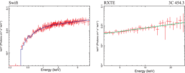
Figure 10: Two $EF_{E}$ spectral diagrams during the LHS (2009 September, 18, blue line, left panel) and the LHS (1996 November, 2 (green line, right panel)). Data taken from $Swift$ observation 00031493003 (low/hard state) and from the RXTE observation, 20346-01-01-00 ($R2$ set, low/hard state).

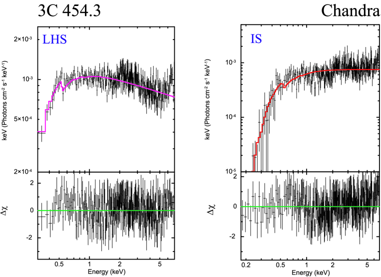
Figure 11: Two representative EF(E) spectral diagrams, for different states of 3C 454.3. Data are taken from $Chandra$ observations ID=4843 (left panel, LHS) and ID=3127 (right panel, HSS). The data are shown by black crosses and the spectral model (tbabs*BMC) is displayed as a colored line.

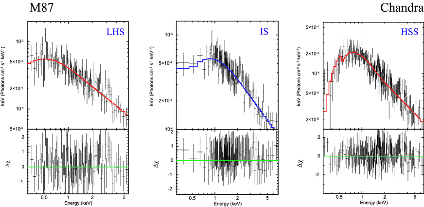
Figure 12: Three representative energy spectra for different states of M87. Data were taken from $Chandra$ observations ID=11514 (left panel, LHS), ID=21075 (central panel, IS), and ID=18783 (right panel, HSS). The data are shown by black crosses and the spectral model (tbabs*BMC) is displayed as a colored line.

Figure 12 shows three representative spectra for different states of M87. These Chandra energy spectra demonstrate an evolution of the source from the low/hard state to the softer states which was observed in the particular dates of 2010, 2016 and 2018 (see Table 6).

We use the geometry for the X-ray spectral formation in 3C 454 and M87 shown in Seifina et al. (2018b); see Fig. 7 there. Regarding this geometry and taking into account our X-ray spectral analysis, we see that that the soft (disk) photons illuminate the Compton cloud (CC) surrounding a BH hole, and matter from the CC is accreted onto the BH following a converging flow (the Bulk Comptonization region).

In Figure 13 we present the evolution of the X-ray properties of 3C 454.3. One can see that the photon indices change in the range from 1.3 to about 1.8 when the corresponding normalization slightly increases. These spectral evolution was observed by the RXTE during 1996 – 1997 outburst transition events ($R1$–$R2$).

In addition, we present the evolution of the optical and X-ray properties of 3C 454.3 (Fig. 14): the optical light curve (in stellar magnitudes) of 3C 454.3 (top panel), the RXTE/ASM count rate, and the BMC normalization during the outburst event of 2009 – 2010 ($R5-R6$ sets). In the bottom panel, we see again the slight change of the photon index $\Gamma=\alpha+1$. The high X-ray flux (MJD 55550) is seen when the optical flux is low. At the same time, during the optical flash at MJD=55200 we see correlation of the optical flux in all filters (top panel). It is important to conclude that the optical variability (e.g., MJD 55400 – 55550) is weakly related to X-ray variability. This could indicate that the origins of the optical and X-ray emissions are different.

Applying the Suzaku data (see black triangles in Figure 15) we obtain that the photon index, $\Gamma,$ monotonically increases from 1.5 to 2.0 when the normalization of the BMC component (or mass accretion rate) changes by a factor of 10. We illustrate this index versus mass accretion rate behavior in Fig. 15 using RXTE, Swift, Suzaku, and Chandra observations (red squares, blue squares, black triangles, and green points, respectively).

3.3.2 X-ray spectral modeling

As a result of the model selection (see Sect. 3.3.1), we assume one model to fit all spectral data (Tables 1 $-$ 7). We briefly reiterate the physical picture described by the Comptonization model (see Titarchuk et al. (1997), ST09, and Appendix A), and its basic assumptions and parameters. The BMC Comptonization spectrum is the sum of the portion of the blackbody emission directly seen by the Earth observer [a fraction of $1/(1+A)$] and a fraction of the blackbody, $f=A/(1+A)$, convolved with the up-scattering Green’s function, $G(E,E_{0})$ which is, in the BMC model, a broken power-law:

$$F_{\nu}=N_{BMC}[(1-f)*BB(E)+f*\int_{0}^{\infty}BB(E_{0})G(E,E_{0})dE_{0}].$$ (5)

It is worth emphasizing that this Green’s function is characterized by the main parameter, the spectral index $\alpha=\Gamma-1$. As one can see, the BMC model has the parameters, $\alpha$, $A$, the seed blackbody temperature $T_{s},$ and the blackbody normalization, which is proportional to the seed blackbody luminosity and inversely proportional to $D^{2}$ where $D$ is the distance to the source. We also apply a multiplicative Tbabs component characterized by an equivalent hydrogen column $N_{H}$ in order to take into account absorption by neutral material.

Figures 9 and 13 show the spectral evolution from the LHS to the IS. The BMC model successfully fits the 3C 454.3 spectra for all spectral states. The $Swift$ spectrum obtained for 3C 454.3 in its IS using the BMC model is shown in Fig. 8. In Table 2 (at the bottom), we present the results of spectral fitting $Suzaku$ data of 3C 454.3 using our main spectral model tbabs*bmc.

Applying the RXTE data (see Tables 7, LABEL:tab:par_rxte_2010), we find the LHS$-$IS transition that is related to the photon index evolution, when $\Gamma$ changes from 1.2 to 2.1 with an increase of the seed photon normalization (proportional to the mass accretion rate). For the RXTE fits, we fix the seed photon temperature at 200 eV. The BMC normalization, $N_{BMC}$, varies by a factor of 100, in the range of $0.1<N_{BMC}<10\times L_{35}/d^{2}_{10}$ erg s^-1 kpc^-2. The Comptonized (illumination) fraction changes only slightly around $\log{A}\sim$ 1.5 [$f=A/(1+A)$].

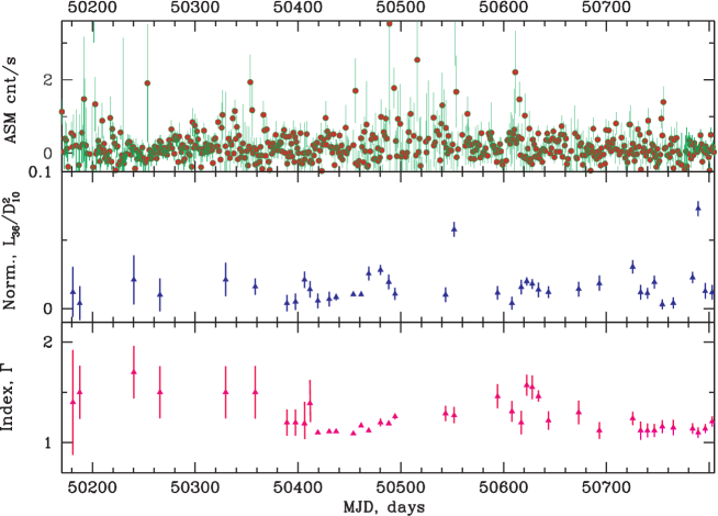
Figure 13: Top: Evolution of the RXTE/ASM count rate for 3C 454. Middle: BMC normalization for 3C 454 during 1996 – 1997 outburst events ($R1-R2$ sets). Bottom: Evolution of the photon index $\Gamma=\alpha+1$.

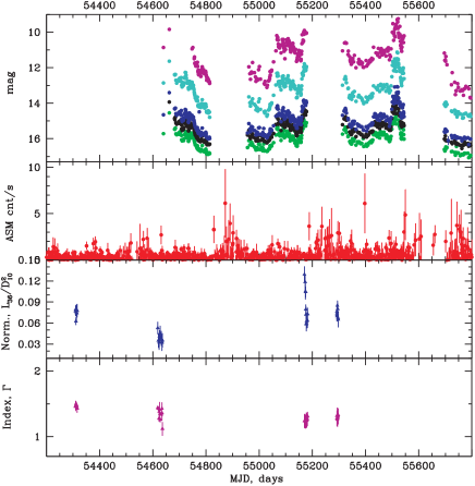
Figure 14: Top: Evolution of the optical flux (in stellar magnitudes) of 3C 454.3 in B-filter (green), V-filter (black), R-filter (blue), J-filter (bright blue), and K-filter (pink). Second row: RXTE/ASM count rate. Third row: BMC normalization during 2009 – 2010 outburst events ($R5-R6$ sets). Bottom: Evolution of the photon index $\Gamma=\alpha+1$.

As discussed above, the spectral evolution of 3C 454.3 was previously investigated using X-ray data by many authors. In particular, Abdo et al. (2010) and Raiteri et al. (2011) studied the 2008 ($Suzaku$), 2008–2009 ($Swift$), and 2008 – 2010 ($Swift$) data sets, respectively (see also Tables 1 and 5), using single power law and absorbed power-law models, respectively. It is worth noting that Abdo et al. (2010) and Raiteri et al. (2011) fixed the hydrogen column to $N_{H}=1.67\times 10^{21}$ cm^-2 and $N_{H}=1.34\times 10^{21}$ cm^-2, respectively (applying the $Chandra$ observations in 2005, see Villata et al. 2006) These qualitative models were used to establish the evolution of the spectral model parameters throughout state transitions during the outbursts.

We also found similar spectral behavior using our model and the full set of the $RXTE$ observations. In particular, like in the aforementioned Guainazzi’s and Rivers’s et al works, we also found that 3C 454.3 demonstrates a change of the photon index $\Gamma$ between $\sim$1.2 and 2.1 during the LHS – IS transition. Furthermore, we revealed that $\Gamma$ tends to saturate at 2.1 at high values of $N_{bmc}$. In other words we find that $\Gamma$ saturates at 2.1 when the mass accretion rate increases.

Our spectral model shows very good performance throughout all data sets. In Tables 2, LABEL:tab:par_rxte$-$LABEL:tab:par_rxte_2010, and Figures 8$-$11 and 13$-$14 we demonstrate the good performance of the BMC model in application to the $Chandra$, $Swift$, $Suzaku,$ and $RXTE$ data for which the reduced $\chi^{2}_{red}=\chi^{2}/N_{dof}$ ($N_{dof}$ is the number of degree of freedom) is less than or around 1 for all observations ($0.75<\chi^{2}_{red}<1.19$).

We performed a similar simulation of the M87 spectrum using the available observations. The RXTE data reveal a weak activity of the M87 nucleus in X-rays. However, for 13 years there is a set of all states from the LHS to the HSS. In particular, M87 spends most of its time in the HSS (1997–1998, $\Gamma\sim 3$), although it can slowly reach LHS (2010, $\Gamma\sim 1.7-1.9$). The data of two other satellites fill the gaps between these states. $ASCA$ (1993) and $Suzaku$ (2006) find the M87 core in the IS ($\Gamma\sim 2.5$). Finally, $BeppoSAX$ (1996) points to the LHS ($\Gamma\sim 1.6$).

In Table 8 we present the results of spectral fitting $Chandra$ data of M87 using our main spectral model tbabs*bmc. Using the RXTE data (see Table LABEL:tab:par_rxte_m87) the LHS$-$IS transition is related when $\Gamma$ changes from 1.8 to 3 and the normalization of the seed photon increases. For the RXTE fits we fix the seed photon temperature at 200 eV. The BMC normalization, $N_{BMC}$, varies by a factor of five in the range of $0.33<N_{BMC}<1.5\times L_{37}/d^{2}_{10}$ erg s^-1 kpc^-2.

As we have already discussed above, the spectral evolution of M87 was previously investigated using X-ray data by many authors. In particular, Abdo et al. (2010) and Raiteri et al. (2011) studied data sets from 2008 ($Suzaku$) and 2008–2009 ($Swift$), and 2008 – 2010 ($Swift$), respectively (see also Tables 1 and 5), using a single power law and an absorbed power-law model, respectively. For their spectral analysis, Abdo et al. (2010) and Raiteri et al. (2011) used the hydrogen column fixed to $N_{H}=1.67\times 10^{21}$ cm^-2 and $N_{H}=1.34\times 10^{21}$ cm^-2, respectively, as determined by the $Chandra$ observations in 2005 and Villata et al. 2006. These qualitative models describe the evolution of these spectral model parameters throughout the state transition during the outbursts.

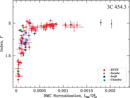
Figure 15: 3C 454: Correlations of photon index $\Gamma$ ($=\alpha+1$) vs. BMC normalization, $N_{BMC}$ (proportional to mass accretion rate) in units of $L_{39}/D^{2}_{10}$. Red and blue squares show $RXTE$ and $Swift$ observations, respectively, while blue triangles and green points correspond to Suzaku and Chandra observations, respectively.

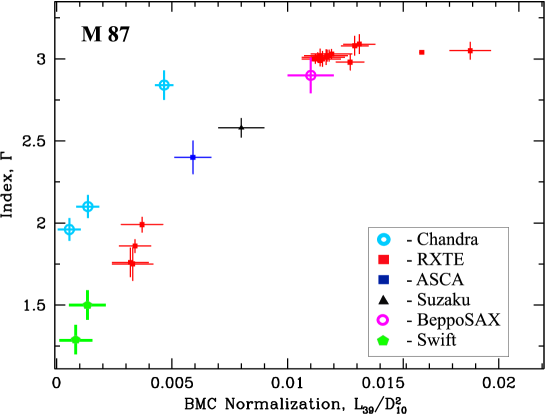
Figure 16: M87: Correlations of photon index $\Gamma$ ($=\alpha+1$) vs. BMC normalization, $N_{BMC}$ (proportional to mass accretion rate) in units of $L_{39}/D^{2}_{10}$. Red and blue squares show $RXTE$ and $ASCA$ observations, respectively, green points correspond to the Swift observations, black triangles correspond to $Suzaku$ data, a pink circle denotes a point related to $BeppoSAX$ observations, and blue circles show those related to $Chandra$ observations.

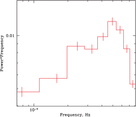
Figure 17: Representative power spectrum of M87. Data are taken from $RXTE$/ASM observations (1996–2011) with a time bin of 100 ks.

We estimated a radius of the blackbody emission region, $R_{BB}$, using a relation $L_{BB}=4\pi R^{2}_{BB}\sigma T^{4}_{BB}$, where $L_{BB}$ is the seed blackbody luminosity and $\sigma$ is the Stefan-Boltzmann constant. With a distance $D$ to the source of $5\times 10^{3}$ Mpc, we found $R_{BB}\sim 1.6\times 10^{12}$ cm. Such a large black body region would only be expected around a supermassive black hole (SMBH) and therefore 3C 454.3 is probably a SMBH source.

We also observed the photon index, $\Gamma,$ versus the normalization of the X-ray spectrum (proportional to the mass accretion rate) in the case of M87. In this case, $\Gamma$ increases from a value of 1.3 and saturates at 3 (see Fig. 16). The inclusion of high-quality observations using the $Chandra$ data allows us to take into account the radiation of the nucleus only (without outer AGN parts and jet contaminations). In Figure 15 we can see that $Chandra$ observations for 3C 454.3 (green points) agree well with the general $\Gamma$–Norm trend, while for M87, Chandra observations (blue points) show a slightly lower normalization for the same photon indices (see Fig. 16) along with that for RXTE, $Suzaku,$ and $Swift$ points.

4 Discussion

The spectral data of 3C 454.3 and M87 are accurately fitted by the BMC model for all analyzed LHS and IS spectra (see Figures 8–10 and Tables 2, LABEL:tab:par_rxte and LABEL:tab:par_rxte_2010). Our results of spectral analysis are consistent with previous results of the spectral fitting by other authors using various X-ray observations of 3C 454.3 and M87.

In particular, Rivers et al. (2011) found a value for $\Gamma$ of about 1.5 on average using the RXTE data of 3C 454.3, while Giommi et al. (2006) obtained $\Gamma\sim 1.7$ using $Swift$ observations of 3C 454.3. Chitnis et al. (2009) showed that $Swift$ spectra of 3C 454.3 can be fitted by an absorbed power-law model with $\Gamma$ of 1.3 using the $Swift$ data. Rivers et al. (2013) demonstrated that soft X-ray emission can be described by an absorbed power law with $\Gamma\sim 1.6$ using the RXTE data. Raiteri et al. (2008) showed that $\Gamma$ changes from 1.5 to 1.6 using the appropriate XMM-$Newton$ observations. Raiteri et al. also found $\Gamma$ to vary from 1.38 to 1.85, with an average value of $\Gamma\sim 1.6$ based on $Swift$ data obtained in 2008–2010 (Raiteri et al. 2011). $Susaku$ observations also demonstrated that $\Gamma=1.58\pm 0.01$ for 2008 observations (our $Sz1$ state, see Table 2). The combined $IBIS$ and $Jem-X$ data of 3C 454.3 obtained onboard $INTEGRAL$ gave $\Gamma=1.8$ (Pian et al. 2006). Finally, Pacciani et al. (2010) found that $\Gamma$ was very close to 1.7 using the RXTE data and $\Gamma=1.5-1.7$ using $Swift$/XRT observations of 3C 454.3.

For M87, Wilson and Yang (2002) described the spectrum of the nucleus obtained using Chandra by a simple power-law model and found that the values of the photon index vary from 2 to 3, which is in good agreement with our results.

4.1 Timing analysis

We examined archival RXTE/ASM observations of M87 obtained from January 6, 1996, to December 28, 2011. The ASM light curve is presented in the top panel of Figure 6. This light curve was analyzed using the powspec task from FTOOLS 6.26.1. We generated power density spectra (PDSs) in the $10^{-7}-10^{-3}$ Hz frequency range and subtracted the contribution due to Poissonian statistics for all PDSs. To model PDSs we used the QDP/PLT plotting package. The PDS continuum shape is usually characterized by band-limited noise shape, which is well presented by an empirical model $P_{X}\sim(1.0+(x)^{2})^{-in}$ ($KING$ model in QDP/PLT plotter). The parameter $in$ is a slope of PDS continuum. As a result, we find a statistically significant ($3\sigma$) feature at the frequency $\nu_{max}\sim 5\times 10^{-7}$ Hz (see Fig. 17) with a time bin of $\sim$100 ks. One can estimate an upper limit of a BH mass magnitude using this PDS feature as follows

$$\nu_{max}\sim V_{pl}/L_{tr}=10^{8}\frac{[V_{pl}/(10^{8}\leavevmode\nobreak\ \rm{cm/s})]}{L\leavevmode\nobreak\ (\rm cm)}\leavevmode\nobreak\ {\rm cm/s},$$ (6)

where $L_{tr}$ is the size of the Compton cloud (CC) in centimeters (or the transition layer) and $V_{pl}$ is a plasma velocity in the CC of the order of $10^{8}$ cm/s related to a typical plasma temperature of the order of 10 keV (see Shaposhnikov & Titarchuk 2009). We use a value of the maximum of $\nu*$ PDS frequency which is $\sim 5\times 10^{-7}$ Hz in order to estimate a BH mass in M87:

$$L_{tr}\sim\frac{V_{pl}}{\nu_{max}}\sim 2\times 10^{14}\leavevmode\nobreak\ \frac{V_{pl}/10^{8}\leavevmode\nobreak\ {\rm cm/s}}{\nu_{max}/5\times 10^{-7}\leavevmode\nobreak\ {\rm Hz}}\leavevmode\nobreak\ {\rm cm}.$$ (7)

One can easily compare this size $L_{tr}$ with the Schwarzschild radius $R_{\rm S}$ and find that

$$M_{87}<L/R_{{\rm S},\odot}\sim 0.6\times 10^{9}\leavevmode\nobreak\ {\rm solar\leavevmode\nobreak\ masses}.$$ (8)

This BH estimate in M87 is at least one order of a magnitude lower than that obtained by other methods for M87 [see Akiyama et al. (2019)]. In Sect. 4.3 we show that $m_{87}=M_{87}/M_{\odot}$ can be more precisely obtained using the scaling method.

4.2 Saturation of the index as a signature of a BH

We applied our analysis in order to find the evolution of $\Gamma$ in 3C 454.3 and M87, and found that $\Gamma$ saturates with the mass accretion rate, $\dot{M}$. ST09 demonstrates this index saturation is an indication of the converging flow (CF) into a BH. In fact, the spectral index $\alpha\sim Y^{-1}$is inverselly proportional to the Comptonization parameter, $Y$ which is a product of an average number of scatterings N in the CF and an efficiency of the energy gain at any scattering in average $\eta$ [see Laurent & Titarchuk (2007)]. But for the converging flow the efficient number of scattering, $N$ is proportional to the dimensionless mass accretion rate $\dot{m}$ [or the optical depth $\tau$, not like $\tau^{2}$ in the thermal plasma, see e.g. Rybicki & Lightman (1979)] and the energy gain $\eta\propto{\dot{m}^{-1}}$. Thus one obtains that $\alpha$ saturates when $\dot{m}$ increases. This is precisely what we see in Figs. (18-19). Another words, when the normalization parameter, proportional the mass accretion rate, $\dot{m}$ increases the photon index $\Gamma=\alpha+1$ saturates. Titarchuk & Zannias (1998), hereafter TZ98, semi-analytically discovered this saturation effect. Later Laurent & Titarchuk (1999), (2011) (hereafter LT99 and LT11, respectively) confirmed it using Monte Carlo simulations.

It should be also noted that Titarchuk, Lapidus & Muslimov (1998), hereafter TLM98, demonstrated that the innermost part of the accretion flow (the so-called transition layer) shrank when $\dot{M}$ increased.

Observations of many Galactic BHs (GBHs) and their X-ray spectral analysis (see ST09, Titarchuk & Seifina (2009), Seifina & Titarchuk (2010) and Seifina et al. (2014); hereafter STS14) confirm this TZ98 prediction. For 3C 454.3, we also reveal that $\Gamma$ monotonically increases from 1.2 and then finally saturates at a value of 2.1 (see Figure 15 for 3C 454.3). For M87, the photon index increases from 1.3 and then saturates at 3. The index-$\dot{M}$ correlations found in 3C 454.3 and M87 allow us to estimate BH masses in these sources by scaling these correlations with those detected in a number of GBHs and extragalactic sources (see details below in Sect. 4.3 and in Appendix B).

Table 9: Parameterizations for reference and target sources

Reference source	$\cal A$	$\cal B$	$\cal D$	$x_{tr}$	$\beta$
GRO J1655–40	2.03$\pm$0.02	0.45$\pm$0.03	1.0	0.07$\pm$0.02	1.9$\pm$0.2
Cyg X–1	2.09$\pm$0.01	0.52$\pm$0.02	1.0	0.4$\pm$0.1	3.5$\pm$0.1
NGC 4051	2.05$\pm$0.07	0.61$\pm$0.08	1.0	[9.54$\pm$0.2]$\times 10^{-4}$	0.52$\pm$0.09
NGC 7469	2.04$\pm$0.06	0.62$\pm$0.03	1.0	1.25$\pm$0.04	0.62$\pm$0.04
XTE J1550-564 RISE 1998	2.84$\pm$0.08	1.8$\pm$0.3	1.0	0.132$\pm$0.004	0.61$\pm$0.02
H 1743-322 RISE 2003	2.97$\pm$0.07	1.27$\pm$0.08	1.0	0.053$\pm$0.001	0.62$\pm$0.04
4U 1630-472	2.88$\pm$0.06	1.29$\pm$0.07	1.0	0.045$\pm$0.002	0.64$\pm$0.03
M101 ULX-1	2.88$\pm$0.06	1.29$\pm$0.07	1.0	[4.2$\pm$0.2]$\times 10^{-4}$	0.61$\pm$0.03
ESO 243-49 HLX-1	3.00$\pm$0.04	1.27$\pm$0.05	1.0	4.25$\pm$0.03	0.62$\pm$0.05
Target source	$\cal A$	$\cal B$	$\cal D$	$x_{tr}$	$\beta$
3C 454.3	2.01$\pm$0.06	0.60$\pm$0.03	1.0	[1.2$\pm$0.2]$\times 10^{-4}$	0.60$\pm$0.04
M87	3.02$\pm$0.07	0.52$\pm$0.02	1.0	[0.8$\pm$0.1]$\times 10^{-4}$	0.50$\pm$0.03

4.3 An estimate of BH mass in 3C 454.3 and M87

A previous mass estimate of a central engine in 3C 454.3 was made using a spectroscopic method applied to multi-wavelength data (see Gupta et al., 2017; Woo & Urry 2002; Liu et al. 2006; Sbarrato et al. 2012; Gu et al. 2001). Particularly, Gupta et al. estimated a BH mass of 3C 454.3 (see also Vestergaard & Osmer 2009) using optical emission (the broad Mg II line width and the continuum luminosity at 3000 Å). We estimated a BH mass, $M_{BH}$, in 3C 454.3 applying X-ray data. In order to estimate $M_{BH}$ we chose two Galactic sources [GRO J1655–40, Cygnus X–1 (see ST09)] and an extragalactic source (NGC 4051; Seifina et al. 2018, hereafter SCT18) as the reference sources, whose BH masses and distances are well established now.

A BH mass for GRO J1655–40 was estimated using dynamical methods. For a BH mass estimate of 3C 454.3 we also used the BMC normalizations, $N_{BMC}$ of these reference sources. As a result, we scale the index versus $N_{BMC}$ correlations for the target and reference sources, NGC 4051 and NGC 7469 (see Figure 18). The value of the index saturation is almost the same, $\Gamma\sim 2$ for all these target and reference sources. We apply the correlations found in these four reference sources to make a comprehensive cross-check of a BH mass estimate for 3C 454.3.

For M87, a BH mass estimate turns out to be highly dependent on the accuracy of the distance to it. The distance to M87 has been estimated using several independent techniques which include measurement of the luminosity of planetary nebulae, comparison with nearby galaxies for which a distance is estimated using standard candles such as cepheid variables, and the linear size distribution of globular clusters (SBF method). This yields a distance of 16.6$\pm$2.3 Mpc (Blakeslee et al. 2009). Furthermore, the tip of the red-giant branch method (Bird et al., 2010) using individually resolved red giant stars (TRGB method) yields a distance of 16.7$\pm$0.9 Mpc (Bird et al., 2010)]. It should be noted that the SBF measurements by Blakeslee et al. (2009) used the HST ACS-VCS data, while the TRGB measurements were based on data from the Next Generation Virgo Cluster Survey (NGVCS) obtained using ground-based adaptive-optics with the Canada French Hawaii Telescope (Cantiello et al. 2018).

These SBF and TRGB measurements are consistent with each other, and their weighted averages yield a distance of 16.4$\pm$0.5 Mpc (Bird et al., 2010). Using this distance and the modeling of surface brightness and stellar velocity dispersion at optical wavelengths (Gebhardt & Thomas 2009; Gebhardt et al. 2011), a BH mass for M87 of $6.2_{-0.6}^{+1.1}\times 10^{9}$ M_⊙ was inferred (Akiyama et al., 2019). On the other hand, mass measurements modeling the kinematic structure of the gas disk (Harms et al. 1994; Macchetto et al. 1997) give us a BH mass of $3.5_{-0.3}^{+0.9}\times 10^{9}$ M_⊙ (Walsh et al. 2013). Therefore, a wide range of SMBH mass estimates exist from $(3.5\pm 0.8)\times 10^{9}$ M_⊙ (Walsh et al., 2013) to $(6.6\pm 0.4)\times 10^{9}$ M_⊙ (Walsh et al., 2013). This agrees with the BH mass estimate of $7.22^{+0.34}_{-0.40}\times 10^{9}$ M_⊙ obtained by Oldham & Auger (2016). In April 2019, the the Event Horizon Telescope (EHT) observations released measurements and estimates of a BH mass as (6.5 $\pm$ 0.2${}_{stat}\pm$ 0.7_sys) $\times 10^{9}$ M_⊙ (Akiyama et al., 2019), which is also consistent with the above estimates.

However, it is desirable to use an identification for the core of M87 that is as independent as possible, as well as a BH mass estimate that uses an alternative to the above-mentioned methods, such as the scaling technique (ST09).

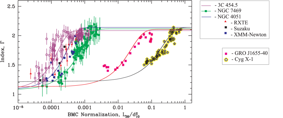
Figure 18: Scaling of the photon index $\Gamma$ vs. the normalization $N_{BMC}$ for 3C 454.3 (violet line – target source) as well as NGC 4051, NGC 7469, GRO J1655–40, and Cygnus X–1 (reference sources). Red triangles stand for RXTE, black squares – $Suzaku$ and blue squares for XMM-$Newton$ data for NGC 4051, while green squares mark RXTE data for NGC 7469. Pink squares and yellow-black circles correspond to RXTE data for GRO J1655–40 and Cygnus X–1, respectively.

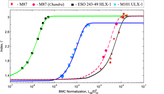
Figure 19: Scaling of the photon index $\Gamma$ vs. the normalization $N_{BMC}$ for M87 (black line – target source) using Galactic sources: XTE J1550–564, 4U 1630–472 and H 1743–322 (reference sources). Pink crosses stand for RXTE data of 4U 1630–472, green circles mark H 1743–322 data, and blue squares indicate XTE J1550–564 data. Pink dashed line indicates the $\Gamma$-Norm correlation corrected for a nucleus emission from M87 using $Chandra$ data ($pink$ points). For the scaling of a BH mass of M87 we used this corrected $\Gamma$-Norm track (see details in the text).

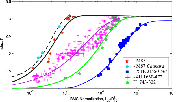
Figure 20: Scaling of the photon index $\Gamma$ vs. the normalization $N_{BMC}$ for M87 (black line – target source) using extragalactic sources: ESO 243–49 HLX–1 and M 101 ULX–1 (reference sources). Black squares stand for RXTE data of ESO 243–49 HLX–1 and blue triangles indicate M 101 ULX–1 data. The black dashed line indicates the $\Gamma$-Norm correlation corrected for a nucleus emission from M87 using $Chandra$ data (bright blue points). For the scaling of BH mass of M87 we used this corrected $\Gamma$-normalization track.

The BH mass scaling process is described in detail in Appendix B. This method can be used to (i) search for such pairs of black holes for which the $\Gamma$ increases with $\dot{M}$ (the BMC normalization, $N_{BMC}$ ) along the $\Gamma-N_{BMC}$ track and those for which the saturation level $\Gamma_{sat}$ is the same, and to ii) calculate two scaling coefficients which allows determination of the BH mass of a target.

As can be seen from Figs. 18, 19, and 20, the correlations of the target sources (3C 454.3 and M87) and the reference sources are characterized by similar shapes and index saturation levels. Consequently, this method gives us a reliable scaling of these correlations with that of 3C 454.3 and M87. In order to implement the scaling technique we introduce an analytical approximation of the $\Gamma-N_{bmc}$ correlation, fitted by Eq. (16).

As a result of fitting the observed correlation by this function $F(x)$ [see Eq. (16)] we obtained a set of the best-fit parameters $\cal A$, $\cal B$, $\cal D$, $N_{tr}$, and $\beta$ (see Table 9). The meaning of these parameters is described in detail in our previous papers (Titarchuk & Seifina (2016), hereafter TS16; STU18; SCT18). This function $F(x)$ is widely used for a description of the correlation of $\Gamma$ versus $N_{bmc}$ (Sobolewska & Papadakis (2009), ST09, Seifina & Titarchuk (2010), STS14, Giacche et al. (2014), Titarchuk & Seifina 2016, 2017; Seifina et al. 2017, 2018a,b).

In order to implement this BH mass determination for the target source one should rely on the same shape of the $\Gamma-N_{BMC}$ correlations for this target source and those for the reference sources. Accordingly, the only difference in values of $N_{bmc}$ for these three sources is in the ratio of the BH mass to the squared distance, $M_{BH}/d^{2}$. As one can see from Fig.  18 the index saturation value, $\cal A,$ is approximately the same for the target and reference sources (see also the second column in Table 9). The shape of the correlations for 3C 454.3 (violet line) and Cyg X–1 (black line) are similar and the only difference between these correlations is in the BMC normalization values (proportional to $M_{BH}/d^{2}$ ratio).

To estimate a BH mass, $M_{t}$, of 3C 454.3 and M87 (target sources) one should slide the reference source correlation along the$N_{BMC}-$axis to that of the target source (see Figs. 18, 19 and 20):

$$m_{t}=m_{r}\frac{N_{t}}{N_{r}}\left(\frac{d_{t}}{d_{r}}\right)^{2}f_{G}=m_{r}\frac{N_{t}}{N_{r}}\left(\frac{z_{t}}{z_{r}}\right)^{2}f_{G},$$ (9)

where $m_{t}=M_{t}/M_{\odot}$, $m_{r}=M_{r}/M_{\odot}$ are the dimensionless BH masses with respect that of the sun, and  $z_{r}$, $z_{t}$ are redshifts of the reference and target sources, correspondingly.

In Figure 18 we demonstrate the $\Gamma-N_{bmc}$ correlation for 3C 454.3 (violet points) obtained using the $RXTE$ spectra along with the correlations for the two Galactic reference sources (GRO J1655–40 (pink), Cygnus X–1 (black)) and two extragalactic reference source (NGC 4051 (green line) and NGC 7469 (blue line)), which are similar to the correlation found for the target source.

For M87, we performed scaling with both galactic and extragalactic sources. Specifically, Fig. 19 presents $\Gamma$ versus normalization, $N_{BMC}$ for M87 (black line – target source) along with $\Gamma$-Norm correlations for extragalactic sources, ESO 243–49 HLX–1 and M 101 ULX–1 (reference sources). It can be seen that the $Chandra$ points go to the left with respect of other points, perhaps due to the fact that we applied a more compact angular region around the nucleus of M87 for the $Chandra$ spectra. Figure 20 shows the photon index $\Gamma$ versus the normalization $N_{BMC}$ for M87 along with $\Gamma-N_{BMC}$ correlations for four Galactic reference sources: XTE J1550–564, 4U 1630–472 and H 1743–322. The black line indicates the $\Gamma-N_{BMC}$ correlation corrected for a nucleus emission from M87 using the $Chandra$ data. For an estimate of a BH mass in M87 we use this corrected $\Gamma-N_{BMC}$ track. The BH masses and distances for each of these target-reference pairs are shown in Table 10.

We apply values of $m_{r}$, $m_{t}$, $d_{r}$, $d_{t}$, and $\cos(i)$ (see Table 10) and then we calculate the the BH mass for 3C 454.3 using the best-fit value of $N^{3c}_{t}=(1.2\pm 0.1)\times 10^{-4}$ taken at the beginning of the index saturation (see Fig. 18) and measured in units of $L_{39}/d^{2}_{10}$ erg s^-1 kpc^-2 (see Table 9 for values of the parameters of function $F(N_{t})$ (Eq. 1)).

For M87, the best-fit value is $N^{m87}_{t}=(0.8\pm 0.1)\times 10^{-4}$. Using $d_{r}$, $m_{r}$, $N_{r}$ (see ST09) we found that $C_{0}\sim 2.0,2.0,1.9,$ and $1.83$ for NGC 7469, NGC 4051, GRO J1555–40, and Cyg X–1, respectively (for 3C 454.3 case). Similarly, we obtained that $C_{0}\sim 1.9,2.0,2.1,$ and $2.03$ for XTE J1550–564, H 1743–322, GRS 1915+105 and 4U 1630–472, respectively.

We find that $M_{3C}\geq 3.4\times 10^{9}\leavevmode\nobreak\ M_{\odot}$ ($M_{3C}=M_{t}$) assuming $d_{3C}\sim$ 3$\times 10^{3}$ Mpc (Gupta et al., 2017; Wright, 2006). To determine the distance to 3C 454.3 we used the formula

$$d_{3c}=z_{3c}c/H_{0},$$ (10)

where the redshift $z_{3c}=0.859$ for 3C 454.3 (see Wright 2006), $c$ is the speed of light, and $H_{0}=70.8\pm 1.6$ km s^-1 Mpc^-1 is the Hubble constant. For M87 case, we obtain $M_{87}\geq 5.6\times 10^{7}\leavevmode\nobreak\ M_{\odot}$ ($M_{87}=M_{t}$) assuming $d_{m87}\sim$ 16.8 Mpc (Akiyama et al., 2019).

It is worth noting that for M87, we take into account the correction (dashed line) of the $\Gamma$-Normalization of the track. This correction for the jet contamination is important in the case of M87. In fact, for a reliable BH mass estimate we need to use the nucleus emission to scale the $\Gamma$-$N_{BMC}$ correlations. In addition, we selected reference sources with a well-known geometric factor (i.e., the angles at which we see the source). This allowed us to obtain a more accurate estimate of the BH mass and not just its lower limit. It should also be emphasized that the BH mass value in M87 turned out to be two orders of magnitude smaller than that estimated by standard methods [see e.g., Akiyama et al. (2019)]. We summarize all these results in Table 10.

In addition, we tested the possible contribution from the broad-line region (BLR). To disentangle this contribution we investigated the low-energy part of the $Chandra$ spectrum of 3C 454.3 (which was calculated for an angular region that captures only the core) and compared it with the $Suzaku$ spectrum of 3C 454.3 (which captures both the core region and the jet region and the BLR zone). As a result, we find that few photons come from the jet and BLR zone in this range. Therefore, the contribution of BLR is small.

Celotti et al. (2007) argued that blazar spectra are contributed via the bulk Compton process by a cold, relativistic shell of plasma moving (and accelerating) along the jet of a blazar, scattering external photons emitted by the accretion disk and reprocessed in the BLR zone. However, the bulk Comptonization of disk photons provide a spectral component contributing in the far-ultraviolet band, and are therefore currently unobservable. On the other hand, the bulk Comptonization of broad-line photons may yield a significant feature in the soft X-ray band. Such a feature is rather transient however, and only dominates over the nonthermal continuum when: (i) the dissipation occurs close to, or within, the BLR; and (ii) other competing processes, like the synchrotron self-Compton emission, yield a negligible flux in the X-ray band. The presence of a bulk Compton component may account for the X-ray properties of high-redshift blazars that show a flattening (and possibly a hump) in the soft X-rays, previously interpreted as due to intrinsic absorption.

We also tested $Suzaku$ and $Chandra$ data and concluded that the spectra of 3C454.3 are even less influenced by jet. In fact, the $Chandra$ spectra focused on a compact area around the nucleus of 3C 454.3 (without the jet contamination), while $Suzaku$ spectra come from some wider zone (nucleus plus jet and outer parts of the AGN). We analyzed and compared these $Suzaku$ and $Chandra$ spectra. As a result, we concluded that the jet contribution (SSC+CE) is too low for the observations used in the paper.

The obtained BH mass estimate is in agreement with a high bolometric luminosity for 3C 454.3 and the $kT_{s}$ value which is in the range of 100–260 eV using the Suzaku and $Chandra$ spectra. For example, Shakura & Sunyaev, (1973) and Novikov & Thorne, (1973) provide an effective temperature of the accretion material, $T_{eff}\sim T_{s}\propto M_{BH}^{-1/4}$.

It is also important to emphasize that our BH mass estimate in 3C 454.3 is consistent with a SMBH mass of $(0.5-1.5)\times 10^{9}$ M_⊙ (Gupta et al., 2017; Woo & Urry 2002; Liu et al. 2006; Sbarrato et al. 2012; Gu et al. 2001). The derived BH mass is the lower limit estimate only because the photon index versus the normalization has the uncertainty with geometrical factor $f_{G}=(\cos i_{d})_{r}/(\cos i_{d})_{t}$. Generally, the photon index versus the QPO frequency correlation enables us to obtain the precise BH mass (see ST09). Although our BH mass estimate is only the lower limit of that, it significantly constrains the BH mass for 3C 454.3 (see Table 10).

Table 10: Black hole masses and distances

Source	Mdyn (M${}_{\odot})$	iorb (deg)	d (kpc)	$M_{lum}$ (M⊙)	Mscal (M⊙)
GRO J1655–40	6.3$\pm$0.3(1,2)	70$\pm$1(1,2)	3.2$\pm$0.2(3)	…
Cyg X–1	6.8 – 13.3(4,5)	35$\pm$5(4,5)	2.5$\pm$0.3(4,5)	…	7.9$\pm$1.0
NGC 4051(6,7,8,9,10)	…	…	$\sim$10$\times 10^{3}$	…	$\geq 6\times 10^{5}$
NGC 7469(11,12,13)	…	…	$\sim$70$\times 10^{3}$	…	$\geq 3\times 10^{6}$
XTE J1550-564(14,15,16)	9.5$\pm$1.1	72$\pm$5	$\sim$6	…	10.7$\pm$1.5c
H 1743-322(17)	…	75$\pm$3	8.5$\pm$0.8	…	13.3$\pm$3.2c
GRS 1915+105(18)	…	60-70	8.5$\pm$0.8	…	13.3$\pm$3.2c
4U 1630–47(19)	…	$\leq$70	$\sim$10 – 11	…	9.5$\pm$1.1
M101 ULX-1(20,21,22,23,24)	3 – 1000	60(25)	(6.4$\pm$0.5)$\times 10^{3}$,	…	$\geq 3.2\times 10^{4}$, $\geq 4.3\times 10^{4}$
			(7.4$\pm$0.6)$\times 10^{3}$
ESO 243-49 HLX-1(26,27)	…	70(28)	$\sim$95$\times 10^{3}$	8$\pm 4\times 10^{4}$	$\geq 7.2\times 10^{4}$
3C 454.3(29)	…	$\leq$4(29)	$\sim$30$\times 10^{5}$	…	$\sim 3.4\times 10^{9}$
M87(30,31)	…	$\leq$20(31)	(16.8$\pm$ 0.8) $\times 10^{3}$	6.5$\pm$ 0.7 $\times 10^{9}$	$\sim$ 5.6 $\times 10^{7}$

(1) Green et al. 2001; (2) Hjellming & Rupen 1995; (3) Jonker & Nelemans G. 2004 (4) Herrero et al. (1995); (5) Ninkov et al. (1987); (6) M^cHardy et al. (2004); (7) Haba et al. (2008); (8) Pounds & King (2013); (9) Lobban et al. (2011); (10) Terashima et al. (2009); (11) Peterson et al. (2004); (12) Peterson et al. (2014); (13) Shapovalova et al. (2017); (14) Orosz et al. 2002; (15) S$\grave{a}$nchez-Fern$\grave{a}$ndez et al. 1999; (16) Sobczak et al. 1999; (17) Petri 2008; (18) Mirabel & Rodrigues 2007 (19) King et al. 2014 (20) STS14; (21) Shappee & Stanek 2011; (22) Mukai et al. 2005; (23) Kelson et al. 1996; (24) TS15; (25) Liu et al. 2013; (26) Copperwheat et al. 2007; (27) Farrell et al, 2009; (28) Soria et al. 2013 (29) Gupta et al. (2017); (30) Akiyama et al. 2019a (31) Davis et al. 2011

We derived the bolometric luminosity using the normalization of the BMC model and found it to be between $2\times 10^{46}$ erg/s and $4\times 10^{47}$ erg/s (assuming isotropic radiation). Observations of many Galactic BHs (GBHs) and their X-ray spectral analysis (see ST09, Titarchuk & Seifina (2009), Seifina & Titarchuk (2010) and STS14, SCT18, STU18) confirm the TZ98 prediction that the spectral (photon) index saturates with the mass accretion rate, the latter being related to the Eddington ratio. This value is not so far from the Eddington limit for the obtained BH mass and assumed source distance (see Table 10).

The resulting mass of the central BH in 3C 454.3 is in agreement with previous estimates of a BH mass (Gupta et al., 2017; Woo & Urry 2002; Liu et al. 2006; Sbarrato et al. 2012; Gu et al. 2001). At the same time its high value raises the question of the origin of such SMBHs and their high variability. The answer to this question can be given by a timing analysis using the longest interval of observations. There are indications of a duality of the central object (Volvach et al., 2017), which may partly manifest itself in the form of a high variability of its radiation and; updated scenarios and justification for feeding such a system of two BHs are however needed. Further observations of 3C 454.3 in a different range of frequencies could shed light on these and other problems.

5 Conclusions

We found the spectral state transitions observed in 3C 454.3 and M87 using the full set of $Suzaku$ (2007 – 2010), $Swift$ (2005 – 2009), RXTE (1996 – 2010), $Chandra$, $ASCA,$ and $Beppo$SAX data and demonstrated a validity of the spectral BMC model for fitting the observed spectra for all these sets of observations, independently of the spectral state of the sources.

We investigated the X-ray flaring properties of 3C 454.3 and M87 and revealed spectral state transitions during the outbursts using the index$-$normalization (proportional to $\dot{M}$) correlation observed in 3C 454.3 and M87, which were similar to those in Galactic BHs as well as in a number of extragalactic BH sources. In particular, we find that 3C 454.3 follows the $\Gamma-\dot{M}$ correlation previously obtained for extragalactic SMBH sources, NGC 4051 (SCT18), NGC 7469 (STU18), Galactic BHs GRO J1655–40, and Cyg X–1 (ST09) for which we take into account the particular values of the $M_{BH}/d^{2}$ ratio (see Fig. 18). We find that M87 follows the $\Gamma-\dot{M}$ correlation previously obtained for extragalactic IMBHs, ESO 243–49 HLX–1 (ST16a) and M 101 ULX-1 (TS16b), and Galactic BHs, XTE J1550–564, 4U 1630–472, GRS 1915+105, and H 1743–322 (ST09) which we use as reference sources, for which we take into account the particular values of the $M_{BH}/d^{2}$ ratio (see Figs. 19 and 20).

The photon index $\Gamma$ of the 3C 454.3 spectra is in the range of $\Gamma=1.2-2.1$, while the photon index $\Gamma$ of the M87 spectra varies in the range of $\Gamma=1.3-3.1$. We tested a possible effect of the presence of the jet for 3C 454.3 and M87 on our results using $Chandra$ observations. We conclude that the jet contribution in the spectrum is relatively small in the case of 3C 454.3, but can contribute to the M87 spectra. Therefore, to estimate the BH mass for M87, it was crucial to separate the radiation of the nucleus and the jet.

We also find that the peak bolometric luminosity for 3C 454.3 is about $2\times 10^{46}$ erg s^-1. We use the observed index–mass accretion rate correlation to estimate $M_{BH}$ in 3C 454.3. This scaling method was successfully applied to find BH masses of Galactic (e.g. ST09, STF13) and extragalactic BHs (TS16; Sobolewska & Papadakis (2009); Giacche et al. (2014); Titarchuk & Seifina (2017); Seifina et al. 2017, 2018a,b). Applying the scaling technique to the X-ray data for Suzaku, Swift, $Chandra$, $ASCA$, $Beppo$SAX, and RXTE observations of 3C 454.3 and M87 allows us to estimate $M_{BH}$ for these particular sources. We find values of $M_{BH}\sim 3.4\times 10^{9}M_{\odot}$ (for 3C 454.3) and $M_{BH}\sim 5.6\times 10^{7}M_{\odot}$ (for M87).

It must also be emphasized that the mass of the BH in M87 estimated in this paper ($M^{m87}_{BH}\sim 5.6\times 10^{7}M_{\odot}$) turned out to be two orders of magnitude smaller than that estimated by standard methods (Gebhardt & Thomas 2009; Gebhardt et al. 2011; Akiyama et al. (2019)) that indicate a BH mass for M87 of $\geq 6\times 10^{9}$ M_⊙. This discrepancy in BH mass estimates for M87 poses a problem to observers and theorists. However, the power spectrum lead us to lower the BH mass in M87 (see Sect. 4.1).

Our BH mass estimate for 3C 454.3 on the other hand is in agreement with the previous BH mass evaluations of $0.5-4.5\times 10^{9}$ M_⊙ derived using different BH mass estimate methods and multiwavelength observations (Gupta et al., 2017; Woo & Urry 2002; Liu et al. 2006; Sbarrato et al. 2012; Gu et al. 2001). Combining all these estimates with the inferred low temperatures of the seed disk photons $kT_{s}$ we establish that the compact object of 3C 454.3 is likely to be a SMBH with at least $M^{3c}_{BH}>3.4\times 10^{9}M_{\odot}$.

Appendix A Comptonized spectrum using the BMC model

The BMC model describes the outgoing spectrum as a convolution of the input “seed” blackbody-like spectrum, whose normalization is $N_{BMC}$ and color temperature is $kT$, with the Comptonization Green’s function. It was realized a long time ago (see e.g., Titarchuk et al. (1997); Shrader & Titarchuk (1998); Laurent & Titarchuk (1999), hereafter LT99) that one should compute the expected spectral energy distribution for an accreting BH and neutron star binaries in terms of only four model parameters: the disk color temperature, a geometric factor related to the illumination of the BH site by the disk, a spectral index related to the efficiency of the Comptonization (thermal or bulk-motion up-scattering), and the normalization (the so-called BMC model). In this case the shape of the emergent spectrum is described by Eq. (5). If we want take into account the recoil effect we should introduce one more parameter $E_{cf}$ which characterizes the high-energy cutoff energy (see the COMPTT or COMPTB models). The BMC analytical model was successfully checked by LT99 and Laurent & Titarchuk (2011) using the Monte Carlo simulations. These latter authors demonstrated that the core of the spectrum, until the recoil high-energy cut-off, is exactly described by the BMC model.

Appendix B The $\Gamma$-normalization correlation and details of the BH mass estimates

The evaluation method of a black holes mass is based on a comparative analysis of similar $\Gamma-N_{BMC}$ tracks by scaling their characteristics. It was shown in Titarchuk & Zannias (1998) and LT99 that the photon index $\Gamma$ monotonically increases with an increase in the accretion rate (which is proportional to the normalization parameter in the Compotonization model; e.g.. COMPTT, COMPTB, BMC) and saturates, i.e., reaches a constant level, with large values of the mass accretion rate $\dot{M}$. The steepness for the $\Gamma-N_{BMC}$ track and the saturation level of $\Gamma_{sat}$ may be different for different black holes. The comparative analysis in the scaling problem is therefore simplified as searching for such pairs of black holes for which the rate of $\Gamma$ increases with $\dot{M}$ ($N_{BMC}$) along the $\Gamma-N_{BMC}$ track and the saturation level $\Gamma_{sat}$ is the same. It is assumed that for each BH from such a pair, distances are known. In addition, the mass of one of the black holes of this pair is known. The scaling process itself consists in calculating two scaling coefficients and then with their help the mass of the desired BH is determined.

We now briefly reiterate the main points of the scaling method. Shaposhnikov & Titarchuk (2007), hereafter ST07, apply an inverse proportionality of a frequency of quasi-periodic oscillations (QPO) on BH mass in order to estimate the latter. ST07 also present theoretical arguments in terms of the transition layer model for the inverse proportionality of QPO frequencies on BH mass. Therefore, a first scaling law claims that

$$s_{\nu}=\frac{\nu_{r}}{\nu_{t}}=\frac{M_{t}}{M_{r}},$$ (11)

where subscript $r$ and $t$ subscripts denote reference and target sources.

The second scaling law, which we use as a basis for our scaling technique, is the detected intensity dependence of the source luminosity and distance:

$$\frac{F_{r}}{F_{t}}=\frac{L_{r}}{L_{t}}\,\frac{d^{2}_{t}}{d^{2}_{r}}.$$ (12)

Here, $F$ stands for the source flux detected by an observer on Earth, $L$ is the source luminosity, and $d$ is a source distance. The luminosity $L$ can be represented as

$$L=\frac{GM_{BH}}{R_{*}}\dot{M}\eta\sim\frac{GM_{BH}}{R_{S}}\dot{M}\eta\sim\dot{M}\eta=M_{BH}\dot{m}\eta,$$ (13)

where $R_{*}$ is the effective radius where energy release occurs, $\eta$ is the efficiency of gravitation energy conversion into radiation power, $\dot{M}$ is the accretion rate, and $\dot{m}$ is its dimensionless analog normalized by the Eddington luminosity. Both $\dot{m}$ and $\eta$ are considered to be the same for two different sources and for the same spectral state, which lead us to $L_{r}/L_{t}=M_{r}/M_{t}=1/s_{\nu}$. In our analysis of energy spectra from BHs we determine normalization of seed photon radiation supplied by an accretion flow (disk) prior to Comptonization. The ratio of this normalization for the two sources in the same spectral state can be written as

$$s_{N}=\frac{N_{r}}{N_{t}}=\frac{L_{r}}{L_{t}}\frac{d^{2}_{t}}{d^{2}_{r}}f_{G}.$$ (14)

Here, $f_{G}$ is a geometry factor that comes due to the fact that the accretion disk which produces thermal input for Comptonization has a plane geometry. Therefore, in the case of radiation coming directly from the disk it would have the value $f_{G}=(\cos i_{d})_{r}/(\cos i_{d})_{t}$, where $i_{d}$ is the inclination angle of the disk. When information on a (target and reference) source inclination is available we can use the values $i_{d,r}$ and $i_{d,t}$.

We are now ready to write down the final equations of our scaling analysis. When $s_{N}$ are measured directly using observations, the mass of the target source can be calculated as

$$m_{t}=m_{r}\frac{d_{t}^{2}}{d_{r}^{2}}\frac{f_{G}}{s_{N}}.$$ (15)

This equation allows estimation of a ratio $m_{t}$ using values of $m_{r}$, $s_{N}$, $f_{G}$, $d_{t}$ and $d_{r}$.

Using Eq. (15), the problem of BH mass and distance measurements for a target source is reduced to the determination of scaling coefficients $s_{N}$ with respect to the data for a reference source. This can be obtained by a technique similar to that adopted by ST07. Specifically, after scalable state transition episodes are identified for two sources, the correlation pattern for a reference transition is parameterized in terms of the analytical function (see also ST09),

$$F(x)={\cal A}-({\cal D}\cdot{\cal B})\ln\{\exp[(1.0-(x/x_{tr})^{\beta})/{\cal D}]+1\},$$ (16)

where $x=N_{bmc}$.

After rearrangement, the BH mass $M_{t}$ of a target source can be evaluated using the formula (see TS16)

$$m_{t}=C_{0}{N_{t}}{d_{t}}^{2}f_{G},$$ (17)

where $C_{0}=(1/d_{r}^{2})(m_{r}/N_{r})$ is the scaling coefficient for the reference source, BH masses $m_{t}$ and $m_{r}$ are in solar units, and $d_{r}$ is the distance to a particular reference source measured in kiloparsecs.

Table 11: Best-fit parameters of spectral analysis of RXTE observations of 3C 454.3 ($R1$ – $R2$ sets) in the 3 – 50 keV energy range^†. Parameter errors correspond to 90% confidence level.

Observational ID	MJD	$\alpha=\Gamma-1$	$kT_{s}$	$N_{BMC}^{\dagger\dagger\dagger}$	$\chi^{2}_{red}$ (dof)
	(day)		(keV)	($L_{35}/d^{2}_{10}$)
10360-01-23-00	50358.56	0.63$\pm$0.09	0.5$\pm$0.2	1.6$\pm$0.1	0.75 (49)
10360-01-36-00	50265.65	0.54$\pm$0.09	0.5$\pm$0.2	1.0$\pm$0.2	0.87 (47)
10360-01-27-00	50329.59	0.7$\pm$0.1	0.5$\pm$0.2	2.1$\pm$0.2	0.95 (47)
10360-01-40-00	50240.21	0.76$\pm$0.09	0.7$\pm$0.2	2.1$\pm$0.3	0.87 (49)
10360-01-47-00	50187.57	0.3$\pm$0.2	0.5$\pm$0.2	0.4$\pm$0.1	0.85 (54)
10360-01-48-00	50181.11	0.6$\pm$0.2	0.4$\pm$0.4	1.2$\pm$0.3	0.94 (54)
20346-01-01-00	50389.18	0.4$\pm$0.2	0.2$\pm$0.1	0.4$\pm$0.1	0.85 (54)
20346-01-02-00	50397.65	0.36$\pm$0.07	0.2$\pm$0.1	0.5$\pm$0.1	0.97 (54)
20346-01-03-00	50406.32	0.94$\pm$0.07	0.6$\pm$0.4	2.1$\pm$0.1	0.89 (54)
20346-01-04-00	50411.66	0.53$\pm$0.09	0.8$\pm$0.6	1.4$\pm$0.1	0.76 (54)
20346-01-05-00	50419.32	0.21$\pm$0.10	0.10$\pm$0.01	0.57$\pm$0.09	1.05 (54)
20346-01-07-00	50430.41	0.62$\pm$0.09	0.11$\pm$0.01	0.69$\pm$0.09	1.12 (54)
20346-01-08-00	50437.14	0.61$\pm$0.03	0.11$\pm$0.01	0.83$\pm$0.04	0.83 (54)
20346-01-10-00	50453.87	0.71$\pm$0.05	0.09$\pm$0.01	1.04$\pm$0.02	0.82 (54)
20346-01-11-00	50461.42	0.71$\pm$0.05	0.17$\pm$0.01	1.04$\pm$0.02	0.82 (54)
20346-01-12-00	50468.77	1.01$\pm$0.07	0.12$\pm$0.01	2.56$\pm$0.08	0.95 (54)
20346-01-14-00	50480.36	1.00$\pm$0.08	0.20$\pm$0.03	2.82$\pm$0.06	0.93 (54)
20346-01-15-00	50488.36	0.85$\pm$0.02	0.19$\pm$0.01	1.94$\pm$0.09	0.93 (54)
20346-01-16-00	50494.49	0.81$\pm$0.02	0.26$\pm$0.02	1.07$\pm$0.07	1.12 (54)
20346-01-17-00	50543.51	0.69$\pm$0.08	0.29$\pm$0.06	1.01$\pm$0.09	0.73 (54)
20346-01-18-00	50551.81	0.94$\pm$0.07	0.27$\pm$0.06	5.78$\pm$0.09	0.98 (54)
20346-01-24-00	50594.23	0.69$\pm$0.04	0.46$\pm$0.09	1.16$\pm$0.08	0.95 (54)
20346-01-26-00	50608.24	0.13$\pm$0.09	0.31$\pm$0.08	0.40$\pm$0.08	1.00 (54)
20346-01-27-00	50617.22	0.93$\pm$0.08	0.20$\pm$0.09	1.56$\pm$0.09	0.73 (54)
20346-01-28-00	50622.50	0.58$\pm$0.03	0.57$\pm$0.08	1.99$\pm$0.05	0.92 (54)
20346-01-29-00	50627.83	0.68$\pm$0.06	0.55$\pm$0.09	1.80$\pm$0.06	0.87 (54)
20346-01-30-00	50633.97	0.96$\pm$0.05	0.46$\pm$0.04	1.37$\pm$0.09	0.92 (54)
20346-01-31-00	50643.58	0.77$\pm$0.06	0.22$\pm$0.07	1.20$\pm$0.07	0.87 (54)
20346-01-35-00	50673.14	0.55$\pm$0.05	0.30$\pm$0.09	1.42$\pm$0.09	0.87 (54)
20346-01-38-00	50693.06	0.88$\pm$0.02	0.12$\pm$0.06	1.83$\pm$0.09	0.79 (54)
20346-01-43-00	50725.75	1.00$\pm$0.04	0.24$\pm$0.05	3.05$\pm$0.08	0.90 (54)
20346-01-44-00	50733.43	0.78$\pm$0.06	0.12$\pm$0.07	1.19$\pm$0.09	0.99 (54)
20346-01-45-00	50739.89	0.72$\pm$0.02	0.12$\pm$0.05	1.12$\pm$0.06	0.95 (54)
20346-01-46-00	50746.76	0.71$\pm$0.08	0.12$\pm$0.05	1.93$\pm$0.08	0.91 (54)
20346-01-47-00	50754.55	0.22$\pm$0.02	0.16$\pm$0.05	0.31$\pm$0.06	1.03 (54)
20346-01-48-00	50765.24	0.26$\pm$0.04	0.15$\pm$0.06	0.41$\pm$0.07	1.05 (54)
20346-01-51-00	50783.86	1.03$\pm$0.07	0.14$\pm$0.04	2.27$\pm$0.07	0.96 (54)
20346-01-52-00	50789.39	1.04$\pm$0.03	0.10$\pm$0.04	7.30$\pm$0.09	0.97 (54)
20346-01-53-00	50796.13	0.87$\pm$0.03	0.14$\pm$0.03	1.28$\pm$0.09	0.86 (54)
20346-01-54-00	50802.97	0.69$\pm$0.08	0.21$\pm$0.04	1.19$\pm$0.09	0.99 (54)

Table 12: Best-fit parameters of spectral analysis of RXTE observations of 3C 454.3 ($R3$ – $R5$ sets) in 3 – 50 keV energy range^†. Parameter errors correspond to 90% confidence level.

Observational ID	MJD	$\alpha=\Gamma-1$	$kT_{s}$	log(A)††	$N_{BMC}^{\dagger\dagger\dagger}$	$\chi^{2}_{red}$ (dof)	F1/F${}_{2}^{\dagger\dagger\dagger\dagger}$
	(day)		(keV)		($L_{35}/d^{2}_{10}$)
30264-01-02-00	50816.05	0.94$\pm$0.12	0.38$\pm$0.05	-0.20$\pm$0.04	12.3 0.5	1.14 (46)	35.87/23.97
30264-01-03-00	50825.97	0.53$\pm$0.09	0.42$\pm$0.08	2.00††	1.04 0.07	1.18 (48)	9.26/8.28
30264-01-04-00	50831.97	0.53$\pm$0.03	0.42$\pm$0.09	2.00††	1.03 0.09	1.16 (48)	9.26/8.28
30264-01-05-00	50839.97	0.54$\pm$0.02	0.25$\pm$0.04	2.00††	1.06 0.09	0.95 (48)	11.8/10.4
30264-01-06-00	50846.97	0.39$\pm$0.03	0.19$\pm$0.08	2.00††	1.05 0.08	0.95 (48)	11.8/10.4
30264-01-08-00	50860.97	0.39$\pm$0.03	0.18$\pm$0.05	2.00††	0.66 0.05	0.98 (48)	9.7/9.8
30264-01-09-00	50911.97	0.40$\pm$0.05	0.19$\pm$0.07	2.00††	0.81 0.08	0.96 (41)	11.87/12.0
30264-01-10-00	50916.97	0.39$\pm$0.01	0.18$\pm$0.03	2.00††	0.65 0.06	0.96 (41)	11.86/12.1
30264-01-12-00	50932.97	0.74$\pm$0.03	0.13$\pm$0.02	2.00††	0.90 0.10	0.74 (49)	10.05/8.45
30264-01-13-00	50939.97	0.19$\pm$0.02	0.12$\pm$0.02	2.00††	0.53 0.20	1.16 (49)	10.9/13.2
30264-01-14-00	50945.97	0.18$\pm$0.01	0.12$\pm$0.01	2.00††	0.63 0.18	0.93 (49)	13.1/15.8
30264-01-15-00	50952.97	0.88$\pm$0.02	0.20$\pm$0.01	2.00††	1.07 0.10	0.95 (48)	12.68/8.13
30264-01-17-00	50966.97	0.89$\pm$0.03	0.20$\pm$0.01	2.00††	0.69 0.10	0.95 (48)	12.68/8.13
30264-01-19-00	50980.97	0.30$\pm$0.03	0.22$\pm$0.01	2.00††	0.41 0.09	1.01 (47)	10.58/11.62
30264-01-20-00	50986.51	0.42$\pm$0.05	0.27$\pm$0.01	2.00††	0.34 0.08	0.95 (47)	8.4/8.29
93150-03-01-00	54309.72	0.92$\pm$0.06	0.46$\pm$0.04	2.00††	7.92 0.10	1.06 (45)	7.05/5.21
93150-03-01-01	54309.93	0.95$\pm$0.07	0.47$\pm$0.06	1.99$\pm$0.09	7.69 0.11	0.97 (45)	6.85/5.06
93150-03-01-02	54311.27	0.90$\pm$0.05	0.50$\pm$0.03	1.66$\pm$0.05	6.26 0.09	1.19 (45)	5.72/4.02
93150-03-01-04	54314.60	0.98$\pm$0.02	0.46$\pm$0.03	1.95$\pm$0.08	7.41 0.10	1.13 (45)	6.58/4.83
93150-03-01-06	54313.30	0.97$\pm$0.05	0.48$\pm$0.04	1.51$\pm$0.06	7.51 0.19	1.09 (45)	6.77/4.80
93150-03-02-00	54315.78	0.96$\pm$0.08	0.43$\pm$0.05	1.60$\pm$0.07	7.78 0.16	1.11 (45)	6.86/5.03
93150-03-03-03	54619.15	0.96$\pm$0.09	0.44$\pm$0.02	1.59$\pm$0.06	5.31 0.15	0.72 (45)	4.67/3.42
93150-03-03-05	54621.02	0.95$\pm$0.08	0.43$\pm$0.01	1.63$\pm$0.04	3.53 0.17	0.95 (45)	3.10/2.29
93150-03-04-00	54624.36	0.91$\pm$0.07	0.38$\pm$0.02	1.76$\pm$0.05	3.57 0.16	0.97 (45)	3.05/2.34
93150-03-04-01	54623.85	0.89$\pm$0.06	0.28$\pm$0.04	1.61$\pm$0.09	3.27 0.18	0.79 (45)	2.64/2.18
93150-03-04-02	54625.88	0.88$\pm$0.07	0.41$\pm$0.09	0.93$\pm$0.07	4.12 0.15	1.06 (45)	3.65/2.48
93150-03-04-04	54627.44	0.90$\pm$0.08	0.35$\pm$0.02	0.99$\pm$0.08	4.14 0.13	0.98 (45)	3.54/2.54
93150-03-04-05	54628.12	0.94$\pm$0.07	0.26$\pm$0.03	1.05$\pm$0.09	4.48 0.19	0.94 (45)	3.65/2.86
93150-03-05-02	54632.34	0.92$\pm$0.06	0.34$\pm$0.02	0.89$\pm$0.08	3.82 0.18	0.96 (45)	3.29/2.31
93150-03-05-04	54634.58	0.91$\pm$0.08	0.43$\pm$0.07	0.81$\pm$0.06	3.22 0.19	0.98 (45)	2.93/1.88
93150-03-05-05	54635.18	0.92$\pm$0.09	0.36$\pm$0.09	0.85$\pm$0.02	3.27 0.13	0.96 (45)	2.87/1.95
93150-03-05-06	54636.81	0.93$\pm$0.08	0.12$\pm$0.08	0.70$\pm$0.05	3.54 0.17	0.95 (45)	2.85/2.25
94150-03-01-00	55170.34	0.97$\pm$0.09	0.24$\pm$0.08	0.73$\pm$0.02	12.95 0.19	1.06 45	11.14/7.74
94150-03-01-01	55173.36	0.97$\pm$0.08	0.24$\pm$0.07	0.73$\pm$0.04	11.86 0.18	1.00 45	10.18/7.07
94150-03-01-02	55174.39	0.96$\pm$0.09	0.23$\pm$0.08	0.74$\pm$0.03	10.54 0.19	0.97 45	8.99/6.33
94150-03-01-03	55175.96	0.95$\pm$0.07	0.25$\pm$0.06	0.73$\pm$0.03	7.95 0.12	1.12 (45)	6.85/4.73
94150-03-01-04	55175.19	0.98$\pm$0.05	0.25$\pm$0.05	0.74$\pm$0.02	10.45 0.13	1.13 (45)	8.97/6.25
94150-03-02-00	55176.44	0.94$\pm$0.06	0.28$\pm$0.04	0.75$\pm$0.03	7.23 0.19	1.07 (45)	6.31/4.28
94150-03-02-01	55177.27	0.93$\pm$0.08	0.25$\pm$0.09	0.81$\pm$0.03	5.85 0.17	0.94 (45)	5.01/3.56
94150-03-02-02	55178.19	0.95$\pm$0.07	0.25$\pm$0.08	0.82$\pm$0.04	6.01 0.13	1.09 (45)	5.12/3.67
94150-03-02-03	55179.17	0.95$\pm$0.07	0.25$\pm$0.08	0.82$\pm$0.04	6.29 0.17	1.02 (45)	5.38/3.83
94150-03-02-04	55180.15	0.95$\pm$0.07	0.26$\pm$0.08	0.83$\pm$0.04	6.35 0.14	1.04 (45)	5.51/3.86
94150-03-02-05	55181.19	0.96$\pm$0.08	0.27$\pm$0.08	0.83$\pm$0.02	6.42 0.18	1.06 (45)	5.57/3.91
94150-03-02-06	55182.76	0.97$\pm$0.03	0.31$\pm$0.05	0.79$\pm$0.04	7.28 0.15	0.97 (45)	6.47/4.35
95149-18-01-02	55293.02	0.98$\pm$0.04	0.32$\pm$0.05	0.78$\pm$0.04	7.41 0.13	0.91 (45)	6.61/4.40
95149-18-01-03	55293.38	0.97$\pm$0.05	0.32$\pm$0.09	0.78$\pm$0.05	7.01 0.12	0.97 (45)	6.26/4.16
95149-18-01-05	55294.28	0.98$\pm$0.06	0.26$\pm$0.08	0.80$\pm$0.06	8.52 0.11	0.98 (45)	7.43/5.15
95149-18-01-08	55293.15	0.98$\pm$0.07	0.28$\pm$0.09	0.80$\pm$0.05	7.17 0.15	0.96 (45)	6.30/4.31
95149-18-01-09	55292.89	0.99$\pm$0.04	0.28$\pm$0.05	0.80$\pm$0.06	7.68 0.17	0.98 (45)	6.74/4.62
95149-18-02-00	55295.77	0.98$\pm$0.05	0.29$\pm$0.08	0.78$\pm$0.02	8.02 0.15	0.94 (45)	7.13/4.78
95149-18-02-01	55296.83	0.98$\pm$0.05	0.31$\pm$0.09	0.77$\pm$0.06	6.75 0.13	0.96 (45)	6.06/4.00
95149-18-02-02	55297.29	0.97$\pm$0.08	0.33$\pm$0.07	0.76$\pm$0.04	6.53 0.19	0.97 (45)	5.92/3.84

Table 13: Best-fit parameters of spectral analysis of RXTE observations of M87 ($R1$ – $R2$ sets) in 3 – 50 keV energy range^†. Parameter errors correspond to 90% confidence level.

Observational ID	MJD	$\alpha=\Gamma-1$	$N_{BMC}^{\dagger\dagger\dagger}$	$E_{cut}$	$E_{fold}$	$E_{line}$	$\sigma_{line}$	$N_{line}^{\dagger\dagger\dagger}$	$\chi^{2}_{red}$ (dof)
	(day)		($L_{37}/d^{2}_{10}$)	(keV)	(keV)	(keV)	(keV)
30216-01-01-000	50812.94	2.02$\pm$0.06	1.18$\pm$0.08	3.6$\pm$0.1	9.9$\pm$0.8	6.4$\pm$0.1	0.7$\pm$0.2	0.10$\pm$0.01	0.95(40)
30216-01-01-010	50813.74	2.04$\pm$0.02	1.58$\pm$0.01	7.3$\pm$0.9	4.7$\pm$0.7	6.6$\pm$0.1	0.2$\pm$0.1	0.09$\pm$0.02	0.95(40)
30216-01-01-02	50814.74	2.00$\pm$0.01	1.11$\pm$0.01	6.7$\pm$0.3	4.2$\pm$0.3	6.5$\pm$0.2	0.5$\pm$0.2	0.08$\pm$0.01	0.93(40)
30216-01-02-00	50822.61	2.01$\pm$0.05	1.13$\pm$0.02	7.0$\pm$0.3	3.6$\pm$0.2	6.4$\pm$0.3	0.4$\pm$0.1	0.07$\pm$0.01	0.98(40)
30216-01-02-01	50823.56	1.99$\pm$0.06	1.14$\pm$0.02	7.2$\pm$0.4	3.4$\pm$0.3	6.5$\pm$0.1	0.3$\pm$0.1	0.09$\pm$0.01	0.86(40)
30216-01-02-020	50824.62	2.00$\pm$0.05	1.12$\pm$0.06	6.8$\pm$0.3	3.8$\pm$0.3	6.3$\pm$0.2	0.4$\pm$0.1	0.10$\pm$0.03	0.93(40)
30216-01-03-00	50832.95	2.02$\pm$0.07	1.14$\pm$0.07	7.0$\pm$0.4	3.6$\pm$0.3	6.4$\pm$0.2	0.5$\pm$0.2	0.10$\pm$0.02	0.86(40)
30216-01-03-01	50833.68	2.01$\pm$0.05	1.13$\pm$0.07	6.3$\pm$0.5	5.1$\pm$0.6	6.5$\pm$0.1	0.4$\pm$0.1	0.08$\pm$0.01	0.99(40)
30216-01-03-02	50833.97	2.00$\pm$0.08	1.15$\pm$0.08	6.7$\pm$0.4	4.2$\pm$0.4	6.5$\pm$0.2	0.4$\pm$0.1	0.09$\pm$0.01	0.96(40)
30216-01-03-03	50833.29	2.00$\pm$0.05	1.14$\pm$0.08	6.2$\pm$0.6	5.2$\pm$0.8	6.3$\pm$0.3	0.7$\pm$0.2	0.10$\pm$0.04	0.95(40)
30216-01-03-04	50835.56	2.03$\pm$0.05	1.19$\pm$0.09	4.6$\pm$0.9	7.2$\pm$0.9	6.5$\pm$0.1	0.4$\pm$0.1	0.10$\pm$0.03	0.98(40)
30216-01-04-00	50843.61	2.02$\pm$0.06	1.17$\pm$0.09	6.5$\pm$0.8	4.5$\pm$0.5	6.5$\pm$0.2	0.4$\pm$0.1	0.08$\pm$0.02	0.97(40)
30216-01-04-01	50844.70	2.01$\pm$0.08	1.16$\pm$0.08	6.8$\pm$0.4	4.2$\pm$0.3	6.4$\pm$0.2	0.4$\pm$0.1	0.10$\pm$0.01	0.99(40)
30216-01-04-02	50845.77	2.08$\pm$0.09	1.29$\pm$0.06	7.1$\pm$0.9	4.7$\pm$0.9	6.3$\pm$0.2	0.4$\pm$0.1	0.10$\pm$0.01	0.96(40)
30216-01-04-03	50843.89	2.09$\pm$0.08	1.31$\pm$0.07	7.3$\pm$1.2	4.5$\pm$0.9	6.5$\pm$0.1	0.6$\pm$0.2	0.08$\pm$0.01	0.98(40)
30216-01-04-04	50846.55	2.05$\pm$0.09	1.79$\pm$0.09	7.1$\pm$1.8	7.8$\pm$1.6	6.4$\pm$0.3	0.4$\pm$0.1	0.09$\pm$0.03	0.97(40)
30216-01-04-05	50846.88	1.98$\pm$0.08	1.27$\pm$0.06	6.9$\pm$1.0	5.0$\pm$1.8	6.5$\pm$0.2	0.7$\pm$0.2	0.10$\pm$0.01	0.94(40)
95145-01-01-00	55296.79	0.99$\pm$0.08	0.37$\pm$0.09	2.8$\pm$1.0	3.7$\pm$0.3	6.3$\pm$0.2	0.4$\pm$0.1	0.10$\pm$0.08	0.93(40)
95145-01-01-01	55298.94	0.86$\pm$0.07	0.34$\pm$0.07	3.3$\pm$1.4	3.4$\pm$0.2	6.5$\pm$0.1	0.5$\pm$0.1	0.09$\pm$0.02	0.97(40)
95145-01-01-02	55299.99	0.8$\pm$0.1	0.33$\pm$0.09	2.9$\pm$1.5	3.1$\pm$1.3	6.4$\pm$0.2	0.6$\pm$0.2	0.09$\pm$0.02	1.03(40)
95145-01-01-03	55301.00	0.76$\pm$0.09	0.32$\pm$0.08	3.1$\pm$1.8	3.0$\pm$1.8	6.5$\pm$0.2	0.4$\pm$0.1	0.10$\pm$0.06	0.95(40)