From Luttinger liquids to Luttinger droplets via higher-order bosonization identities

Abstract

We derive generalized Kronig identities expressing quadratic fermionic terms including momentum transfer to bosonic operators and use them to obtain the exact solution for one-dimensional fermionic models with linear dispersion in the presence of position-dependent interactions and scattering potential. In these Luttinger droplets, which correspond to Luttinger liquids with spatial variations or constraints, the position dependences of the couplings break the translational invariance of correlation functions and modify the Luttinger-liquid interrelations between excitation velocities.

I Introduction

An important goal of condensed matter theory is a reliable description of the correlated behavior of electrons which is rooted in the Coulomb interaction between them. In one-dimensional geometries they exhibit a special coherence at low energies:Sénéchal ; Giamarchi (2003) the dispersion can be approximately linearized in the vicinity of the Fermi points $\pm k_{\text{F}}$ as $\epsilon_{k}$ $\simeq$ $\pm v_{\text{F}}(k\pm k_{\text{F}})$, so that the energy $\delta\epsilon$ $=$ $v_{\text{F}}\delta k$ of a particle-hole excitation from $k_{1}$ to $k_{2}$ is a function only of the momentum transfer $\delta k$ $=$ $k_{2}-k_{1}$. By contrast, in higher dimensions the magnitude and relative orientation of the two momenta usually enter into $\delta\epsilon$, leading to a continuum of excitation energies for a given momentum transfer. This coherence in one dimension is prominently featured in the Tomonaga-Luttinger model,Tomonaga (1950); Luttinger (1963) which is based on the approximation that one can regard a physical electron field operator $\Psi(x)$ for a wire of length $L$ at low energies as a sum of two independent fields,

$$\Psi(x) =\sum_{k}\frac{e^{{\text{i}}kx}}{\sqrt{L}}{\cal C}{\vphantom{+}}_{k}=\sum_{\begin{subarray}{c}k>-k_{\text{F}}\\ \lambda=\pm\end{subarray}}\frac{e^{{\text{i}}\lambda(k_{\text{F}}+k)x}}{\sqrt{L}}{\cal C}{\vphantom{+}}_{\lambda(k_{\text{F}}+k)}$$ (1a)

$$\simeq\frac{e^{{\text{i}}k_{\text{F}}x}\psi_{\text{R}}^{\vphantom{+}}(x)+e^{-{\text{i}}k_{\text{F}}x}\psi_{\text{L}}^{\vphantom{+}}(x)}{\sqrt{2\pi}}\,,$$ (1b)

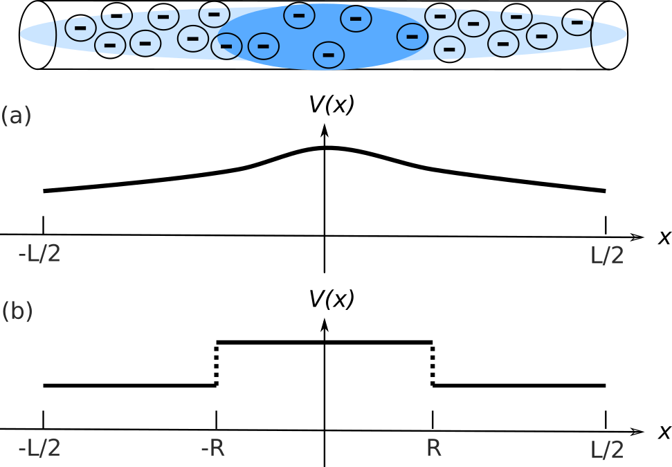
Figure 1: Wire of length $L$ with position-dependent interaction potential $V(x)$ in (4), with $V(x)$ $=$ $V(-x)$, sketched here for the repulsive case with larger $V(x)$ near $x$ $=$ $0$ so that particles tend to keep a larger distance from each other there. An additional single-particle potential $W(x)$ $=$ $W(-x)$ may also be present. (a) A general smooth interaction potential. (b) A piecewise constant interaction potential, i.e., with piecewise constant value $V(0)$ inside and $V(L/2)$ outside a central region of width $2R$, as solved explicitly in Sec. IV.4.4 for $L$ $\to$ $\infty$ and finite $R$.

where the lower summations limits $-k_{\text{F}}$ in (1a) were replaced by $-\infty$ (1b). Then $\psi_{\text{R,L}}^{\vphantom{+}}(x)$ $=$ $\psi_{1,2}^{\vphantom{+}}(\mp x)$ and $\psi_{\eta}^{\vphantom{+}}(x)$ $=$ $(2\pi/L)^{\frac{1}{2}}$ $\sum_{k}{\text{e}}^{-{\text{i}}kx}c^{{\vphantom{+}}}_{k\eta}$ are defined in terms of canonical fermions $c^{{\vphantom{+}}}_{k\eta}$ $=$ ${\cal C}{\vphantom{+}}_{\pm(k_{\text{F}}+k)}$ which correspond to the physical fermions ${\cal C}_{k}$ near the two Fermi points for $\eta$ $=$ $1,2$. In the Tomonaga-Luttinger model the dispersion is linearized near the Fermi points and only forward-scattering density interactions between left- and right-moving fermions are kept. The Tomonaga-Luttinger model can be solved by bosonization,Tomonaga (1950); Luttinger (1963); Mattis and Lieb (1965); Schick (1968); Schotte and Schotte (1969); Mattis (1974); Luther and Peschel (1974); Coleman (1975); Mandelstam (1975); Heidenreich et al. (1975); Haldane (1979); *haldane_luttinger_1981 which expresses the above-mentioned coherence of excitations into an exact mapping to bosonic degrees of freedom (at the operator levelLuther and Peschel (1974); Emery (1979); Voit (1995); Kotliar and Si (1996); von Delft and Schoeller (1998); von Delft et al. (1998); *zarand_analytical_2000 or in a path-integral formulation;Lee and Chen (1988); Yurkevich (2002); Grishin et al. (2004); Galda et al. (2011); Filippone and Brouwer (2016) throughout we use Ref. von Delft and Schoeller, 1998’s constructive finite-size bosonization approach, which is recapped below). Bosonization has led to such remarkable results and concepts as spin-charge separation of elementary excitations,Tomonaga (1950); Luttinger (1963) interaction-dependent exponents of correlation functions,Luther and Peschel (1974); Meden and Schönhammer (1992); *schonhammer_nonuniversal_1993; *schonhammer_erratum:_1993; Meden (1999); Markhof and Meden (2016) and the Luttinger-liquid paradigmHaldane (1981a, 1980); *haldane_demonstration_1981; *haldane_effective_1981 which states that the relations between excitation velocities and correlation exponents of the Tomonaga-Luttinger model remain valid even for weakly nonlinear dispersion. These topics are nowadays presented in many reviewsSénéchal ; Emery (1979); Sólyom (1979); Voit (1995); Schönhammer ; *schonhammer_luttinger_2004; *schonhammer_physics_2013; von Delft and Schoeller (1998); Miranda (2003); Cazalilla et al. (2011) and textbooks.Kopietz (1997); Giamarchi (2003); Gogolin et al. (2004); Bruus and Flensberg (2004); Giuliani and Vignale (2008); Phillips (2012); Mastropietro and Mattis (2013) Characteristic signatures of one-dimensional electron liquids have been observed in a variety of experiments.Milliken et al. (1996); Maasilta and Goldman (1997); Chang (2003); Bockrath et al. (1999); Ishii et al. (2003); Aleshin et al. (2004); Boninsegni et al. (2007); *del_maestro_4he_2011; *duc_critical_2015; Jompol et al. (2009); Barak et al. (2010); Blumenstein et al. (2011); Mebrahtu et al. (2012); *mebrahtu_observation_2013; Yang et al. (2017); Cedergren et al. (2017); Stühler et al. The theory of nonlinear dispersion terms has been of particular further interest,Schick (1968); Haldane (1981a); Busche and Kopietz (2000); *pirooznia_dynamic_2008; Teber (2007); Karrasch et al. (2015) including refermionization techniques which use bosonization identities in reverse to map diagonalized bosonic systems back to free fermions.Rozhkov (2003); *rozhkov_fermionic_2005; *rozhkov_class_2006; *rozhkov_density-density_2008; *rozhkov_one-dimensional_2014; Imambekov and Glazman (2009a); *imambekov_phenomenology_2009; *imambekov_one-dimensional_2012; Teber (2007); Maebashi and Takada (2014); Essler et al. (2015); Markhof et al. (2019) For Luttinger liquids out of equilibriumCazalilla (2006); *iucci_quantum_2009; *nessi_quantum_2013; Uhrig (2009); Foster et al. (2010); Perfetto and Stefanucci (2011); Dziarmaga and Tylutki (2011); Dóra et al. (2011); *dora_generalized_2012; *dora_absence_2015; *dora_momentum-space_2016; Karrasch et al. (2012); *rentrop_quench_2012; Coira et al. (2013); Ngo Dinh et al. (2013); Sabetta and Misguich (2013); Kennes and Meden (2013); *kennes_spectral_2014; Sachdeva et al. (2014); Schiró and Mitra (2015); Mastropietro and Wang (2015) nonlinear dispersion effects are also essential.Gutman et al. (2010); *protopopov_many-particle_2011; *protopopov_relaxation_2014; *protopopov_dissipationless_2014; *protopopov_equilibration_2015; Lin et al. (2013); Buchhold and Diehl (2015a); *buchhold_kinetic_2015; *buchhold_prethermalization_2016; *huber_thermalization_2018

The technical hallmarks of bosonization are the following. On the one hand, a two-body density interaction term for fermions $c^{{\vphantom{+}}}_{k{\eta}}$ becomes quadratic in terms of canonical bosons, defined for $q$ $>$ $0$ as $b^{{\vphantom{+}}}_{q{\eta}}$ $=$ $-{\text{i}}\sum_{k}c^{+}_{k-q{\eta}}c^{{\vphantom{+}}}_{k{\eta}}/\sqrt{\smash[b]{n_{q}}}$. Here the momentum sum runs over $k$ $=$ $\frac{2\pi}{L}(n_{k}-\tfrac{1}{2}\delta_{\text{b}})$ with integer $n_{k}$, and the parameter $0$ $\leq$ $\delta_{\text{b}}$ $<$ $2$ fixes the boundary conditions, $\psi_{{\eta}}^{\vphantom{+}}(x+L/2)$ $=$ ${\text{e}}^{i\pi\delta_{\text{b}}}$ $\psi_{{\eta}}^{\vphantom{+}}(x-L/2)$. On the other hand the fermionic kinetic energy also translates into free bosons by means of the so-called Kronig identity,Kronig (1935); Dover (1968); Schönhammer

$$H_{0{\eta}}^{(1)} =\sum_{k}k\,{}^{\ast}_{\ast}{c^{+}_{k{\eta}}c^{{\vphantom{+}}}_{k{\eta}}}{}^{\ast}_{\ast}$$ (2a)

$$=\sum_{q>0}q\,b^{+}_{q{\eta}}b^{{\vphantom{+}}}_{q{\eta}}+\frac{\pi}{L}(\hat{N}_{{\eta}}+1-\delta_{\text{b}})\hat{N}_{{\eta}}\,,$$ (2b)

where the fermionic number operator is given by $\hat{N}_{{\eta}}$ $=$ $\sum_{k}{}^{\ast}_{\ast}{c^{+}_{k{\eta}}c^{{\vphantom{+}}}_{k{\eta}}}{}^{\ast}_{\ast}$, which commutes with $b^{{\vphantom{+}}}_{q{\eta}}$. The normal ordering ${}^{\ast}_{\ast}{\cdots}{}^{\ast}_{\ast}$ is defined with respect to the state $|{\bm{0}}\rangle_{0}$, where $|{\bm{N}}\rangle_{0}$ is an eigenstate of all $c^{+}_{k{\eta}}c^{{\vphantom{+}}}_{k{\eta}}$ (with eigenvalue 1 if $n_{k}$ $\leq$ $N_{\eta}$ and 0 otherwise). Furthermore, real-space fermionic and bosonic fields are related by the celebrated bosonization identity,Schotte and Schotte (1969); Mattis (1974); Luther and Peschel (1974); von Delft and Schoeller (1998)

$$\psi_{{\eta}}^{\vphantom{+}}(x) =\big{(}\tfrac{2\pi}{L}\big{)}^{\frac{1}{2}}F_{{\eta}}^{\vphantom{+}}\,{\text{e}}^{-{\text{i}}\frac{2\pi}{L}(\hat{N}_{{\eta}}-\frac{1}{2}\delta_{\text{b}})x}\,{\text{e}}^{-{\text{i}}\varphi_{{\eta}}^{+\!}(x)}\,{\text{e}}^{-{\text{i}}\varphi_{{\eta}}^{{\vphantom{+}}}(x)},$$ (3)

which allows the calculation of fermionic in terms of bosonic correlation functions.Luther and Peschel (1974) Here the fermionic Klein factor $F_{{\eta}}^{\vphantom{+}}$ decreases the fermionic particle number $\hat{N}_{{\eta}}$ by one, and $\varphi_{{\eta}}^{{\vphantom{+}}}(x)$ $=$ $-\sum_{q>0}b^{{\vphantom{+}}}_{q{\eta}}\,{\text{e}}^{-{\text{i}}qx-aq}/\sqrt{\smash[b]{n_{q}}}$. The regularization parameter $a$ $\to$ $0^{+}$ is needed to obtain a finite commutator,von Delft and Schoeller (1998) $[\varphi_{{\eta}}^{{\vphantom{+}}}(x),\varphi_{{\eta}}^{+\!}(x^{\prime\!})]$ $=$ $-\ln\!\big{(}1-{\text{e}}^{-\frac{2\pi{\text{i}}}{L}(x-x^{\prime\!}-{\text{i}}a)}\big{)}$. A final ingredient to the solution of the Tomonaga-Luttinger model is a Boguljubov transformation, which absorbs the interaction between left- and right-moving fermions into the free bosonic theory.Tomonaga (1950)

In the present work we will study Luttinger liquids with additional spatial constraints, which we term Luttinger droplets. Namely, we consider a (spinless) fermionic Hamiltonian with linear dispersion, position-dependent interactions $V(x)$ and $U(x)$, and scattering potential $W(x)$ (all assumed to be real symmetric functions of $x$),

$$H =\int\!\frac{\text{d}x}{L}\,{}^{\ast}_{\ast}v_{\text{F}}[\psi_{\text{R}}^{+}(x){\text{i}}\partial_{x}\psi_{\text{R}}^{\vphantom{+}}(x)-\psi_{\text{L}}^{+}(x){\text{i}}\partial_{x}\psi_{\text{L}}^{\vphantom{+}}(x)]$$

$$\,\hphantom{=}\,+W(x)[n_{\text{L}}(x)+n_{\text{R}}(x)]+U(x)n_{\text{L}}(x)n_{\text{R}}(x)$$

$$\,\hphantom{=}\,+\frac{1}{2}V(x)[n_{\text{L}}(x)^{2}+n_{\text{R}}(x)^{2}]{}^{\ast}_{\ast}\,,$$ (4a)

in terms of densities $$n_{\text{R,L}}(x) = \psi_{\text{R,L}}^{+}(x)\psi_{\text{R,L}}^{\vphantom{+}}(x)/(2\pi) W(x) V(x) U(x) H$$ . Without and with constant and , reduces to the usual translationally invariant Tomonaga-Luttinger model (with contact interactions). Below we will diagonalize (4) exactly for the special case

$$U(x) =\gamma\,[2\pi v_{\text{F}}+V(x)]\,,~{}~{}~{}~{}-1<\gamma<1\,,$$ (4b)

for otherwise arbitrary $V(x)$ $>$ $-2\pi v_{\text{F}}$ and a constant $\gamma$. This means that real Fourier components $V_{q}$ $=$ $V_{-q}$ as well as $U_{q=0}$ can be chosen freely; then $\gamma$ $=$ $U_{0}/[2\pi v_{\text{F}}+V_{0}]$ and $U_{q\neq 0}$ $=$ $\gamma V_{q}$. Thus $\gamma$ characterizes the relative strength of interbranch interactions. Below we obtain the single-particle Green function for the ground state of this model, the exponents of which will reflect the spatial dependence of the couplings. We first derive generalized Kronig-type identities in Sec. II, which we then use to solve a single-flavor chiral version of (4) in Sec. III. We then proceed to the two-flavor case in Sec. IV, with a discussion of the similiarities and differences of the spectrum and Green function compared to the translationally invariant case. One representative choice of $V(x)$ to be discussed below involves a central region with stronger repulsion than at the edges of the system, as shown in Fig. 1a. An explicit evaluation is provided for a piecewise constant $V(x)$ as shown in Fig. 1b in Sec. IV.4.4. Relations between the excitation velocities and Green function exponents are discussed in Sec. V, followed by a summary in Sec. VI.

Many results for inhomogeneous Luttinger liquids are of course known, e.g., with barriers,Kane and Fisher (1992a); *kane_transmission_1992; *kane_resonant_1992; Rylands and Andrei (2016); *rylands_quantum_2017; *rylands_quantum_2018 impurities,Meden et al. (2002); Hattori and Rosch (2014) boundaries,Meden et al. (2000); Schneider and Eggert (2010); Rylands leads,Eggert (2000); Filippone and Brouwer (2016) confinementsWonneberger (2001) and so on. Models with (effective) position-dependent Luttinger liquid parameters or interaction potentials have also been investigated.Maslov and Stone (1995); Safi and Schulz (1995); Ponomarenko (1995); Rech and Matveev (2008a); *rech_resistivity_2008; Grishin et al. (2004); *galda_impurity_2011 Our goal is to provide a complementary perspective on these setups with the exact solution of the rather flexible model (4), i.e., the Hamiltonian (4) with parameters from the manifold (4b), and to possibly enable new applications, e.g., to ultradilute quantum droplets held together by weak cohesive forces.Ferrier-Barbut (2019)

II Kronig-type identities with arbitrary momentum transfer

II.1 Bosonic forms of bilinear fermionic terms

Consider a general bilinear fermionic term,

$$H_{q{\eta}}^{(m)} =\sum_{k}k^{m}\,{}^{\ast}_{\ast}{c^{+}_{k-q{\eta}}c^{{\vphantom{+}}}_{k{\eta}}}{}^{\ast}_{\ast}$$ (5a)

$$=\int\!\frac{\text{d}x}{2\pi}\,{\text{e}}^{{\text{i}}qx}\,{}^{\ast}_{\ast}{\psi_{{\eta}}^{+}(x)({\text{i}}\partial_{x})^{m}\psi_{{\eta}}^{\vphantom{+}}(x)}{}^{\ast}_{\ast}\,,$$ (5b)

for integer exponents $m$ $\geq$ $0$ and momentum transfer $q$ $=$ $\frac{2\pi}{L}$ $n_{q}$ with integer $n_{q}$; here and throughout real-space integrals without indicated endpoints extend over the interval $[-L/2,L/2]$. Arbitrary dispersion terms are included in (5a) for $q$ $=$ $0$, such as (2a) for $m$ $=$ $1$. Forming the product of (3) with its hermitian conjugate at different positions $x$ and $x+\ell$, canceling the Klein factors ($F_{{\eta}}^{+}F_{{\eta}}^{\vphantom{+}}$ $=$ $1$), commuting the bosonic fields, taking $a$ to zero, and combining exponentials, we obtain

$$\frac{L}{2\pi}\,\psi_{{\eta}}^{+}(x)\psi_{{\eta}}^{\vphantom{+}}(x+\ell)$$ (6)

$$={\text{e}}^{\pi{\text{i}}(\delta_{\text{b}}-2\hat{N}_{{\eta}})\ell/L}\,{\text{e}}^{{\text{i}}\varphi_{{\eta}}^{+\!}(x)}\,{\text{e}}^{{\text{i}}\varphi_{{\eta}}^{{\vphantom{+}}}(x)}\,{\text{e}}^{-{\text{i}}\varphi_{{\eta}}^{+\!}(x+\ell)}\,{\text{e}}^{-{\text{i}}\varphi_{{\eta}}^{{\vphantom{+}}}(x+\ell)}$$

$$=\frac{{\text{e}}^{\pi{\text{i}}(\delta_{\text{b}}-2\hat{N}_{{\eta}})\ell/L}}{1-{\text{e}}^{2\pi{\text{i}}\ell/L}}\,{\text{e}}^{{\text{i}}(\varphi_{{\eta}}^{+\!}(x)-\varphi_{{\eta}}^{+\!}(x+\ell))}\,{\text{e}}^{{\text{i}}(\varphi_{{\eta}}^{{\vphantom{+}}}(x)-\varphi_{{\eta}}^{{\vphantom{+}}}(x+\ell))}\,,$$

A generating function of the terms in (5a) then reads

$$\sum_{m=0}^{\infty}\frac{(-{\text{i}}\ell)^{m}}{m!}\,H_{q{\eta}}^{(m)}=\sum_{k}{\text{e}}^{-{\text{i}}k\ell}\,{}^{\ast}_{\ast}{c^{+}_{k-q{\eta}}c^{{\vphantom{+}}}_{k{\eta}}}{}^{\ast}_{\ast}$$ (7)

$$=\int\!\frac{\text{d}x}{2\pi}\,{\text{e}}^{{\text{i}}qx}\,{}^{\ast}_{\ast}{\psi_{{\eta}}^{+}(x)\psi_{{\eta}}^{\vphantom{+}}(x+\ell)}{}^{\ast}_{\ast}=\int\!\frac{\text{d}x}{L}\,\frac{{\text{e}}^{\pi{\text{i}}\delta_{\text{b}}\ell/L}\,{\text{e}}^{{\text{i}}qx}}{1-{\text{e}}^{2\pi{\text{i}}\ell/L}}$$

$$~{}~{}~{}\times\,\big{(}{\text{e}}^{-2\pi{\text{i}}\hat{N}_{{\eta}}\ell/L}\,{\text{e}}^{{\text{i}}\varphi_{{\eta}}^{+\!}(x)-{\text{i}}\varphi_{{\eta}}^{+\!}(x+\ell)}\,{\text{e}}^{{\text{i}}\varphi_{{\eta}}^{{\vphantom{+}}}(x)-{\text{i}}\varphi_{{\eta}}^{{\vphantom{+}}}(x+\ell)}-1\big{)}\,,$$

where we summed the Taylor series of the terms (5b), inserted relation (6), and performed the normal ordering. Taylor expanding the exponentials and taking coefficients of $\ell^{m}$ on both sides of (7) now yields $H_{q{\eta}}^{(m)}$ in terms of bosonic operators, as discussed below. Relation (7) thus provides explicit bosonic representations of general bilinear fermionic operators, including (2).

We also introduce operators which use the more convenient powers of the integer $n_{k}$ instead of momentum $k$,

$$\!\!\!\!\!\!\!\!\!\!\!\!\!\!\!\!\!\!\!\!\!\!\!\!K^{\vphantom{(}}_{q{\eta}}(\lambda) =\sum_{k}{\text{e}}^{\lambda n_{k}}\;{}^{\ast}_{\ast}{c^{+}_{k-q{\eta}}c^{{\vphantom{+}}}_{k{\eta}}}{}^{\ast}_{\ast}=\sum_{m=0}^{\infty}\frac{\lambda^{m}}{m!}\,K_{q{\eta}}^{(m)}\,,$$ (8a)

$$K_{q{\eta}}^{(m)} =\sum_{k}n_{k}^{m}\;{}^{\ast}_{\ast}{c^{+}_{k-q{\eta}}c^{{\vphantom{+}}}_{k{\eta}}}{}^{\ast}_{\ast}\,,$$ (8b)

$$K_{q{\eta}}^{(0)} =\sum_{k}{}^{\ast}_{\ast}{c^{+}_{k-q{\eta}}c^{{\vphantom{+}}}_{k{\eta}}}{}^{\ast}_{\ast}=\begin{cases}\phantom{-}\hat{N}_{{\eta}}&\text{\!\!\!\!if\,}n_{q}\!=\!0,\\ \phantom{-}{\text{i}}\sqrt{\smash[b]{n_{q}}}\phantom{{}_{-}}\,b^{{\vphantom{+}}}_{q{\eta}}&\text{\!\!\!\!if\,}n_{q}\!>\!0,\\ -{\text{i}}\sqrt{n_{-q}}\,b^{+}_{-q{\eta}}&\text{\!\!\!\!if\,}n_{q}\!<\!0,\end{cases}\!\!\!\!\!\!$$ (8c)

so that the terms (5a) are then given by $H_{q{\eta}}^{(m)}$ $=$ $(\pi/L)^{m}$ $\sum_{n=0}^{m}$ $\binom{m}{n}$ $(-\delta_{\text{b}})^{m-n}$ $2^{n}$ $K_{q{\eta}}^{(n)}$ and the bosonic commutation relations become $[K_{-q{\eta}}^{(0)},K_{q^{\prime\!}{\eta^{\prime}}}^{(0)}]$ $=$ $-n_{q}\delta_{qq^{\prime\!}}\delta_{{\eta}{\eta^{\prime}}}$. The operators $K^{\vphantom{(}}_{q{\eta}}(\lambda)$, which are operator-valued formal power series in the (complex) indeterminate $\lambda$ with coefficients $K_{q{\eta}}^{(m)}$, obey the intriguing operator algebra

$$\!\!\Big{[}K^{\vphantom{(}}_{-q{\eta}}(\lambda),K^{\vphantom{(}}_{q^{\prime\!}{\eta^{\prime}}}(\lambda^{\prime\!})\Big{]} ={\delta}_{{\eta}{\eta^{\prime}}}\bigg{[}\delta_{qq^{\prime\!}}\frac{{\text{e}}^{-\lambda n_{q}}-{\text{e}}^{\lambda^{\prime\!}n_{q}}}{1-{\text{e}}^{-\lambda-\lambda^{\prime\!}}}$$ (9)

$$~{}~{}~{}+({\text{e}}^{-\lambda n_{q^{\prime\!}}}-{\text{e}}^{\lambda^{\prime\!}n_{q}})K^{\vphantom{(}}_{q^{\prime\!}-q{\eta}}(\lambda+\lambda^{\prime\!})\bigg{]},$$

which is reminiscient of affine Lie algebras,Francesco et al. (1997) but not immediately recognizable. From (7), or alternatively from (9), the generating function (8a) becomes

$$\!K^{\vphantom{(}}_{q{\eta}}(\lambda) =\frac{{\text{e}}^{\lambda\hat{N}_{{\eta}}}Y_{q{\eta}}(\lambda)-\delta_{q0}}{1-{\text{e}}^{-\lambda}}\,,$$ (10a)

$$\!Y_{q{\eta}}(\lambda) =\sum_{n,r=0}^{\infty}\frac{1}{n!r!}\sum_{\begin{subarray}{c}p_{1},\ldots,p_{n}>0\\ p_{1}^{\prime\!},\ldots,p_{r}^{\prime\!}>0\end{subarray}}\delta_{p_{1}+\cdots p_{n}+q,p_{1}^{\prime\!}+\cdots p_{r}^{\prime\!}}$$

$$\;\times\!\Big{(}\prod_{i=1}^{n}\frac{1-{\text{e}}^{-\lambda n_{p_{i}}}}{n_{p_{i}}}K_{-p_{i}{\eta}}^{(0)}\Big{)}\!\Big{(}\prod_{j=1}^{r}\frac{{\text{e}}^{\lambda n_{p_{j}^{\prime\!}}}-1}{n_{p_{j}^{\prime\!}}}K_{p_{j}^{\prime\!}{\eta}}^{(0)}\Big{)}$$

$$=\sum_{m=0}^{\infty}\frac{\lambda^{m}}{m!}Y_{q{\eta}}^{(m)}\,.$$ (10b)

The coefficients $K_{q{\eta}}^{(m)}$ and $Y_{q{\eta}}^{(m)}$ of $\lambda^{m}$ in these expression are given by

$$K_{q{\eta}}^{(m)} =\sum_{m=0}^{\infty}\frac{\lambda^{m}}{m!}\,K_{q{\eta}}^{(m)}=\frac{B_{m+1}(\hat{N}_{{\eta}}+1)-B_{m+1}(1)}{m+1}\delta_{q0}$$

$$+\sum_{n=0}^{m}\binom{m}{n}\frac{(-1)^{n}}{m+1-n}B_{n}(-\hat{N}_{{\eta}})\,Y_{q{\eta}}^{(m+1-n)}\,,$$ (11a)

$$Y_{q{\eta}}^{(m)} =\int\!\frac{\text{d}x}{L}\,{\text{e}}^{{\text{i}}qx}\sum_{n=0}^{m}\binom{m}{n}\mathfrak{B}_{m}\big{(}K_{+{,\eta}}^{(1)\!}(x),...,K_{+{,\eta}}^{(m)\!}(x)\big{)}$$

$$\times\mathfrak{B}_{m}\big{(}K_{-{,\eta}}^{(1)\!}(x),...,K_{-{,\eta}}^{(m)\!}(x)\big{)}\,,$$ (11b)

Here $K_{\pm{,\eta}}^{(m)\!}(x)$ $=$ $\sum_{\pm p>0}n_{-p}^{m-1}K_{-p{\eta}}^{(0)}{\text{e}}^{{\text{i}}px}$ and $B_{n}(x)$ and $\mathfrak{B}_{m}(x_{1},\ldots,x_{m})$ are the Bernoulli and complete Bell polynomials, respectively, defined byComtet (1974)

$$\frac{\lambda\,{\text{e}}^{\lambda x}}{{\text{e}}^{\lambda}-1} =\sum_{m=0}^{\infty}\frac{\lambda^{m}}{m!}B_{m}(x)\,,$$ (12a)

$$\exp\!\bigg{(}\sum_{m=1}^{\infty}\frac{\lambda^{m}}{m!}\,x_{m}\bigg{)} =\sum_{m=0}^{\infty}\frac{\lambda^{m}}{m!}\mathfrak{B}_{m}(x_{1},\ldots,x_{m})\,.$$ (12b)

A detailed derivation of (10)-(11) will be presented elsewhere.

II.2 Bosonic representation of a fermionic scattering term

Generalized Kronig identities for arbitrary order $m$ follow from the equivalence of (8b) and (11a), with the latter involving only fermionic number operators and normal-ordered bosonic operators. As a special case, we obtain for $m$ $=$ $1$ and $q$ $\neq$ $0$ the finite-$q$ generalization of (2),

$$\!\!\!K_{q{\eta}}^{(1)} =\sum_{k}n_{k}\,{}^{\ast}_{\ast}{c^{+}_{k-q{\eta}}c^{{\vphantom{+}}}_{k{\eta}}}{}^{\ast}_{\ast}$$

$$=\Big{(}\frac{n_{q}+1}{2}+\hat{N}_{{\eta}}\Big{)}K_{q{\eta}}^{(0)}+\frac{1}{2}\sum_{p(\neq 0,q)}\!\!K_{q-p{\eta}}^{(0)}K_{p{\eta}}^{(0)}\,,$$ (13)

which can also be expressed as

$$H_{q{\eta}}^{(1)} =\sum_{k}k\,{}^{\ast}_{\ast}{c^{+}_{k-q{\eta}}c^{{\vphantom{+}}}_{k{\eta}}}{}^{\ast}_{\ast}=\frac{2\pi}{L}K_{q{\eta}}^{(1)}-\frac{\pi\delta_{\text{b}}}{L}\hat{N}_{{\eta}}$$ (14a)

$$=\Big{(}\frac{q}{2}+\frac{\pi}{L}(2\hat{N}_{{\eta}}+1-\delta_{\text{b}})\Big{)}\,{\text{i}}\sqrt{\smash[b]{n_{q}}}\,b^{{\vphantom{+}}}_{q{\eta}}$$

$$~{}~{}~{}~{}-\frac{1}{2}\!\sum_{q>p>0}\!\sqrt{(q-p)p}\,b^{{\vphantom{+}}}_{q-p{\eta}}b^{{\vphantom{+}}}_{p{\eta}}$$

$$~{}~{}~{}~{}+\sum_{p>0}\sqrt{p(q+p)}\,b^{+}_{p{\eta}}b^{{\vphantom{+}}}_{q+p{\eta}}\,,~{}~{}~{}~{}(q>0)$$ (14b)

so as to make the modification of the momentum-diagonal identity (2) more apparent.

III Chiral Luttinger droplets

III.1 Droplet model with only right movers

As a simple application of (14) and for later reference we first consider a single species of spinless fermions with density

$$n(x)=\frac{1}{2\pi}\,\psi^{+}(x)\psi^{\vphantom{+}}(x)=\frac{1}{L}\,\sum_{q}K_{q{}}^{(0)}e^{-iqx}\,,$$ (15)

subjected to a single-particle potential $w(x)$ $=$ $w(-x)$ and a position-dependent interaction $g(x)$ $=$ $g(-x)$, with Fourier transforms $w_{q}$ $=$ $\int\!w(x)\,{\text{e}}^{-{\text{i}}qx}\text{d}x/L$ $=$ $w_{-q}$ and so on. For simplicity we choose antiperiodic boundary conditions ($\delta_{\text{b}}$ $=$ $1$). For a linear dispersion the Hamiltonian of such a ‘chiral Luttinger droplet’ is given by

$$H_{\text{chiral}} =v_{\text{F}}\sum_{k}k\,{}^{\ast}_{\ast}{c^{+}_{k{}}c^{{\vphantom{+}}}_{k{}}}{}^{\ast}_{\ast}+\int\!\frac{\text{d}x}{L}\,w(x)\,{}^{\ast}_{\ast}{n(x)}{}^{\ast}_{\ast}$$ (16)

$$\,\hphantom{=}\,+\frac{1}{2}\int\!\frac{\text{d}x}{L}\,g(x)\,{}^{\ast}_{\ast}{n(x)^{2}}{}^{\ast}_{\ast}\,.$$

III.2 Diagonalization of the chiral model

On the one hand, we can now express the fermionic Hamiltonian $H_{\text{chiral}}$ in terms of bosonic operators. We define

$$H_{[\bm{\tilde{g}},\hat{\bm{\tilde{w}}};\bm{K}]}^{\text{bosonic}} =\frac{\tilde{g}_{0}}{L}\sum_{q>0}K_{-q{}}^{(0)}K_{q{}}^{(0)}$$ (17)

$$\,\hphantom{=}\,+\frac{1}{L}\sum_{q\neq 0}\bigg{[}\hat{\tilde{w}}_{q}K_{q{}}^{(0)}+\frac{\tilde{g}_{q}}{2}\!\sum_{p(\neq 0,q)}\!K_{p{}}^{(0)}K_{q-p{}}^{(0)}\bigg{]}\,,$$

with symmetric parameters $\hat{\tilde{w}}_{q}$ (that may contain $\hat{N}$) and $\tilde{g}_{q}$. For $\tilde{g}_{q}$ $=$ $2\pi v_{\text{F}}\delta_{q0}$ $+$ $g_{q}$ and $\hat{\tilde{w}}_{q}$ $=$ $w_{q}L$ $+$ $g_{q}\hat{N}$ we find that

$$H_{\text{chiral}} =H_{[\bm{\tilde{g}},\hat{\bm{\tilde{w}}};\bm{K}]}^{\text{bosonic}}+\frac{\tilde{g}_{0}}{2L}\hat{N}^{2}+w_{0}\hat{N}\,.$$ (18)

On the other hand, the fermionic basis permits a full diagonalization as follows. Using (13) to eliminate the last term in (17) we arrive at a fermionic scattering Hamiltonian,

$$H_{\text{chiral}} =\sum_{kk^{\prime\!}}T_{kk^{\prime\!}}\,{}^{\ast}_{\ast}{c^{+}_{k{}}c^{{\vphantom{+}}}_{k^{\prime\!}{}}}{}^{\ast}_{\ast}\,,$$ (19)

$$T_{kk^{\prime\!}} =v_{\text{F}}k\,\delta_{kk^{\prime\!}}+w_{k^{\prime\!}-k}+(k+k^{\prime\!}\,)\frac{g_{k^{\prime\!}-k}}{4\pi}\,.$$

We conclude that the four-fermion interaction terms in (16) cancel, as they do in the Kronig identity (2). In terms of field operators we obtain

$$H_{\text{chiral}} =\int\!\text{d}x\,{}^{\ast}_{\ast}{\frac{\psi^{+}(x)h(x)\psi^{\vphantom{+}}(x)}{2\pi}}{}^{\ast}_{\ast}\,,$$ (20a)

$$h(x) =\tilde{g}(x)(-{\text{i}}s\partial_{x})-\frac{1}{2}{\text{i}}s\tilde{g}^{\prime\!}(x)+w(x)\,,$$ (20b)

where $\tilde{g}(x)$ $=$ $2\pi v_{\text{F}}$ $+$ $g(x)$ as above, and $s$ $=$ $-1/(2\pi)$.

Next we use the spectrum of the first-quantized Hamiltonian in (20b), $h$ $=$ $s[\tilde{g}(X)P+P\tilde{g}(X)]/2+w(X)$ with $[X,P]$ $=$ i. The eigenvalue equation $h(x)\xi_{k}(x)$ $=$ $E_{k}\xi_{k}(x)$ is separable because $h$ is linear in $P$. For a constant real scale $s$ and real functions $\tilde{g}(x)$, $w(x)$ on an interval $[x_{1},x_{2}]$ with $\tilde{g}(x)$ $>$ $0$ and $\tilde{g}(x_{1})$ $=$ $\tilde{g}(x_{2})$, and demanding $\xi_{k}(x_{2})$ $=$ $\xi_{k}(x_{1}){\text{e}}^{\pi{\text{i}}\delta_{\text{b}}}$, we find $E_{k}$ $=$ $(S_{1}$ $-$ $sLk)/S_{0}$, $\xi_{k}(x)$ $=$ $[\tilde{g}(x)S_{0}]^{-\frac{1}{2}}\exp({\text{i}}[s_{0}(x,0)E_{k}$ $-$ $s_{1}(x,0)]/s)$, where the momentum $k$ takes on the same discrete values $k_{n}$ as before. Here $S_{j}$ $=$ $s_{j}(x_{2},x_{1})$ with $s_{j}(x,x^{\prime})$ $=$ $\int_{x^{\prime}}^{x}\text{d}y\,(\delta_{j0}+\delta_{j1}w(y))/\tilde{g}(y)$. These eigenstates correspond to plane waves subject to a local scale transformation induced by the interaction potential, reminiscient of eikonal wave equations or semiclassical Schrödinger equations. We note the eigenstate expectation values $\langle{w(X)}\rangle$ $=$ $S_{1}/S_{0}$ $=$ $E_{k}-s\langle{P}\rangle$.

Setting $x_{1}$ $=$ $-x_{2}$ $=L/2$ and $\delta_{\text{b}}$ $=$ $1$ and requiring $g_{q=0}$ $>$ $-2\pi v_{\text{F}}$, we thus diagonalize (16), (19), (20) in terms of new canonical fermions, $\{\Xi_{k{}}^{\vphantom{+}},\Xi_{k^{\prime\!}{}}^{+}\}$ $=$ $\delta_{kk^{\prime\!}}$, as

$$H_{\text{chiral}} =\sum_{k}E_{k}\,{}^{\ast}_{\ast}{\Xi_{k{}}^{+}\Xi_{k{}}^{\vphantom{+}}}{}^{\ast}_{\ast}\equiv H_{[\bm{\tilde{g}},\bm{w};\bm{\Xi^{\vphantom{+}}}]}^{\text{diagonal}}\,,$$ (21)

$$E_{k} =\tilde{v}(k-\tilde{k})\,,\,~{}~{}\hat{N}=\sum_{k}{}^{\ast}_{\ast}{\Xi_{k{}}^{+}\Xi_{k{}}^{\vphantom{+}}}{}^{\ast}_{\ast}=\sum_{k}{}^{\ast}_{\ast}{c^{+}_{k{}}c^{{\vphantom{+}}}_{k{}}}{}^{\ast}_{\ast}\,,$$

$$\Xi_{k{}}^{\vphantom{+}} =\int\!\frac{\text{d}x}{\sqrt{2\pi}}\,\xi_{k}(x)\,\psi^{\vphantom{+}}(x)\,,~{}~{}\tilde{k}=-\int\!\frac{\text{d}x}{L}\,\frac{2\pi w(x)}{\tilde{g}(x)}\,,$$

$$\xi_{k}(x) =\frac{\sqrt{2\pi\tilde{v}}\;{\text{e}}^{-{\text{i}}[\tilde{r}_{0}(x)k-\tilde{r}_{1}(x)]}}{\sqrt{L\,\tilde{g}(x)}}\,,~{}\tilde{r}_{0}(x)=\int_{0}^{x}\!\text{d}y\,\frac{2\pi\tilde{v}}{\tilde{g}(y)}\,,$$

$$\tilde{r}_{1}(x) =\tilde{k}\,\tilde{r}_{0}(x)+\int_{0}^{x}\!\text{d}y\,\frac{2\pi w(y)}{\tilde{g}(y)},~{}\tilde{v}=\bigg{[}\int\!\frac{\text{d}x}{L}\,\frac{2\pi}{\tilde{g}(x)}\bigg{]}^{-1}\!.$$

Note that the renormalized dressed Fermi velocity $\tilde{v}$ is given by the spatial harmonic average of the renormalized ‘local’ Fermi velocity $v_{\text{F}}$ $+$ $g(x)/(2\pi)$ $=$ $\tilde{g}(x)/(2\pi)$.

III.3 Green function for the chiral model

From the above solution it is straightforward to obtain the time-ordered Green function for the Heisenberg operators of the chiral field,

$$G(x,x^{\prime\!};t) =\theta(t)G^{>}(x,x^{\prime\!};t)-\theta(-t)G^{<}(x,x^{\prime\!};t)\,,$$ (22)

$$G^{\gtrless}(x,x^{\prime\!};t) =\begin{cases}-{\text{i}}\langle{\psi^{\vphantom{+}}(x,t)\,\psi^{+}(x^{\prime\!},0)}\rangle\,,\\ -{\text{i}}\langle{\psi^{+}(x^{\prime\!},0)\,\psi^{\vphantom{+}}(x,t)}\rangle\,,\end{cases}$$ (23)

with $\theta(\pm t)$ $=$ $(1\pm\text{sgn}(t))/2$. At zero temperature in a state with fixed particle number $N$ we find

$${\text{i}}G(x,x^{\prime\!};t) =\frac{\tilde{v}}{\sqrt{\tilde{g}(x)\tilde{g}(x^{\prime\!})}}\frac{{\text{e}}^{{\text{i}}S(x,x^{\prime},t)}}{\frac{L}{\pi}\sinh\frac{\pi}{L}({\text{i}}R(x,x^{\prime},t)+a\,\text{sgn}\,t)}\,,$$

$$R(x,x^{\prime},t) =\tilde{r}_{0}(x)-\tilde{r}_{0}(x^{\prime})-\tilde{v}t\,,$$ (24)

$$S(x,x^{\prime},t) =\tilde{r}_{1}(x)-\tilde{r}_{1}(x^{\prime})+\tilde{v}\tilde{k}t-\frac{2\pi N}{L}R(x,x^{\prime},t)\,,$$

where $a$ $\to$ $0^{+}$ stems from a convergence factor that was included in the momentum sum. For constant $g(x)$ and $w(x)$ we recover the translationally invariant case, $G(x,x^{\prime\!};t)$ $\propto$ $1/(x-x^{\prime}+\tilde{v}t+a\,\text{sgn}\,t)$, with renormalized Fermi velocity. Position-dependent couplings, on the other hand, may lead to a substantial redistribution of spectral weight. The critical behavior however remains unaffected, in the sense that the exponent of the denominator involving $R(x,x^{\prime},t)$ remains unity for the chiral model.

IV Luttinger droplets

IV.1 Droplet model with with right and left movers

We now study a generalization of the two-flavor Tomonaga-Luttinger model to position-dependent interactions and scattering potentials. Such a ‘Luttinger droplet’ involves right- and left-moving fermions, $\psi_{\text{R}}^{\vphantom{+}}(x)$ $=$ $\psi_{1}^{\vphantom{+}}(-x)$ and $\psi_{\text{L}}^{\vphantom{+}}(x)$ $=$ $\psi_{2}^{\vphantom{+}}(x)$ (see introduction) with linear dispersion in opposite directions, subject to the one-particle potential $W(x)$, as well as intrabranch and interbranch density interactions $V(x)$ and $U(x)$, respectively, as given in (4). In terms of fermions with flavor $\eta$ $=$ $1,2$ we have

$$H={}^{\ast}_{\ast}\sum_{\eta}\Bigg{[}v_{\text{F}}\sum_{k}k\,c^{+}_{k\eta}c^{{\vphantom{+}}}_{k\eta}+\int\!\frac{\text{d}x}{L}\,W(x)n_{\eta}(x)$$

$$~{}~{}+\frac{1}{2}V(x)n_{\eta}(x)^{2}\Bigg{]}+\int\!\frac{\text{d}x}{L}\,U(x)n_{1}(-x)n_{2}(x){}^{\ast}_{\ast}\,,$$ (25)

i.e., compared to (16) the couplings $g(x)$ and $w(x)$ were relabeled as $V(x)$ and $W(x)$, indices $\eta$ were put on operators, and the interaction term with $U(x)$ was included.

IV.2 Diagonalization of the Luttinger droplet model

IV.2.1 Bosonic form of the Hamiltonian

Rewritten with bosonic operators this becomes

$$H =H_{\text{TL}}+H^{\prime}+H^{\prime\prime}\,,$$ (26)

$$H_{\text{TL}} =\sum_{\eta}\bigg{[}\frac{2\pi v_{\text{F}}+V_{0}}{L}\bigg{(}\frac{\hat{N}_{\eta}^{2}}{2}+\sum_{q>0}K_{-q\eta}^{(0)}K_{q\eta}^{(0)}\bigg{)}\bigg{]}$$

$$\,\hphantom{=}\,+\frac{U_{0}}{L}\bigg{[}\hat{N}_{1}\hat{N}_{2}+\sum_{q>0}\bigg{(}K_{-q1}^{(0)}K_{-q2}^{(0)}+K_{q1}^{(0)}K_{q2}^{(0)}\bigg{)}\bigg{]},$$

$$H^{\prime} =\sum_{\eta}\bigg{[}W_{0}\hat{N}_{\eta}+\sum_{q\neq 0}\bigg{(}W_{q}+\frac{V_{q}}{L}\hat{N}_{\eta}+\frac{U_{q}}{2L}\hat{N}_{\bar{\eta}}\bigg{)}K_{q\eta}^{(0)}\bigg{]},$$

$$H^{\prime\prime} =\sum_{\eta}\sum_{q\neq 0}\sum_{p(\neq 0,q)}\!\!K_{p\eta}^{(0)}\bigg{[}\frac{V_{q}}{2L}K_{q-p\eta}^{(0)}+\frac{U_{q}}{2L}K_{p-q\bar{\eta}}^{(0)}\bigg{]}\,.$$

$H$ contains a standard (i.e., translationally invariant) Tomonaga-Luttinger model $H_{\text{TL}}$ involving only the zero-momentum (space-averaged) couplings, which by itself can be diagonalized by a Bogoljubov transformation. For position-dependent couplings, on the other hand, also $H^{\prime}$ (linear in bosons) and $H^{\prime\prime}$ (quadratic in bosons with momentum transfer) are present.

IV.2.2 Specialization to common spatial dependence

For simplicity we set from now on

$$\binom{V(x)}{U(x)} =\binom{V_{0}}{U_{0}}+\binom{V}{U}\sum_{q\neq 0}f_{q}\cos(qx)\,,$$ (27)

with constant prefactors $V$ and $U$ and $f_{q}$ $=$ $V_{q}/V$ $=$ $U_{q}/U$ $=$ $f_{-q}$ for $q$ $\neq$ $0$. We can then simplify the momentum-offdiagonal term $H^{\prime\prime}$ by a Bogoljubov transformation to $K_{q\sigma}^{(0)}$ (for $q$ $\neq$ $0$, $\sigma$ $=$ $-\bar{\sigma}$ $=$ $\pm$, letting $\eta_{\sigma}$ $=$ $(3$ $-$ $\sigma)/2$, $\sigma_{\eta}$ $=$ $3$ $-$ $2\eta$ for $\eta$ $=$ $3$ $-$ $\bar{\eta}$ $=$ $1,2$),

$$K_{q\sigma}^{(0)} ={u}\,K_{q\eta_{\sigma}}^{(0)}+{v}\,K_{-q\bar{\eta}_{\sigma}}^{(0)}\,,$$ (28a)

$$K_{q\eta}^{(0)} ={u}\,K_{q\sigma_{\eta}}^{(0)}-{v}\,K_{-q\bar{\sigma}_{\eta}}^{(0)}\,,$$ (28b)

$u$ $=$ $\cosh\!\theta$, $v$ $=$ $\sinh\!\theta$, which preserves the bosonic algebra, $[K_{-q\sigma}^{(0)},K_{q^{\prime\!}\sigma^{\prime\!}}^{(0)}]$ $=$ $-n_{q}\delta_{qq^{\prime\!}}\delta_{\sigma\sigma^{\prime\!}}$. The choice $U/V$ $=$ $\mathop{\text{tanh}}2\theta$, assuming $|U|$ $<$ $V$, yields

$$H =\sum_{\sigma=\pm}\big{(}H_{\sigma}^{(0)}+H_{\sigma}^{(1)}\big{)}+H^{(2)}+\hat{H}_{\text{N}}+E_{0}\,,$$ (29)

$$\!\!\!\!H_{\sigma}^{(0)} =\frac{\bar{V}}{L}\sum_{q>0}K_{-q\sigma}^{(0)}K_{q\sigma}^{(0)}+\sum_{q\neq 0}\frac{\bar{U}\!f_{q}}{2L}\sum_{p(\neq 0,q)}\!\!K_{p\sigma}^{(0)}K_{q-p\sigma}^{(0)}\,,$$

$$\!\!\!\!H_{\sigma}^{(1)} =\frac{1}{L}\sum_{q\neq 0}\hat{\bar{w}}_{q\sigma}K_{q\sigma}^{(0)}\,,~{}~{}~{}~{}H^{(2)}=\frac{\bar{V}^{\prime}}{L}\sum_{q\neq 0}K_{q+}^{(0)}K_{q-}^{(0)}\,,$$

$$\hat{H}_{\text{N}} =\frac{2\pi v_{\text{F}}+V_{0}}{2L}\sum_{\eta}\hat{N}_{\eta}^{2}+\frac{U_{0}}{L}\hat{N}_{1}\hat{N}_{2}+W_{0}\sum_{\eta}\hat{N}_{\eta}$$ (30)

where $E_{0}$ is a constant energy shift, omitted from now on, which diverges due to the contact interactions in $H$. Here and below we use the following abbreviations and relations,

$$\bar{V} =\frac{(2\pi v_{\text{F}}+V_{0})V-U_{0}U}{\bar{U}}\,,~{}~{}\bar{U}=\bar{\gamma}V,~{}$$ (31)

$$\bar{V}^{\prime} =\frac{U_{0}V-(2\pi v_{\text{F}}+V_{0})U}{\bar{U}}\,,$$

$$\hat{\bar{w}}_{q\sigma} =LW_{q}{\text{e}}^{-\theta}+\bar{\gamma}\,V_{q}\big{[}{u}^{3}\hat{N}_{1}\delta_{\sigma+}-{v}^{3}\hat{N}_{2}\delta_{\sigma-}\big{]},~{}(q\neq 0)\!\!$$

$$\gamma =\frac{U}{V}=\mathop{\text{tanh}}\!2\theta\,,~{}\bar{\gamma}=\sqrt{1-\gamma^{2}}=\text{sech}{2\theta}\,,$$

$$\gamma_{3} =u^{3}-v^{3}=(1+\tfrac{1}{2}\gamma)(1-\gamma)^{-\frac{1}{4}}(1+\gamma)^{-\frac{3}{4}}\,,$$

$${\text{e}}^{-\theta} =(V-U)^{\frac{1}{4}}(V+U)^{-\frac{1}{4}}=(1-\gamma)^{\frac{1}{4}}(1+\gamma)^{-\frac{1}{4}}\,,$$

$$2v^{2} =2\sinh^{2}\!\theta=(1-\gamma^{2})^{-\frac{1}{2}}-1\,.$$

The Hamiltonian $H$ has thus become diagonal in the new flavors $\sigma$ except for the term $H^{(2)}$ in (29).

IV.2.3 Specialization to interrelated interaction strengths

For simplicity we now assume that $\bar{V}^{\prime}$ $=$ $0$, i.e., that the bare Fermi velocity $v_{\text{F}}$ and the strengths of the position-averaged ($V_{0}$ and $U_{0}$) and position-dependent interactions ($V$ and $U$) combine so that $H^{(2)}$ is absent. This corresponds to the special case

$$\gamma =\frac{U}{V}=\frac{U_{0}}{2\pi v_{\text{F}}+V_{0}}\,,$$ (32)

which together with (27) is equivalent to (4b). From now on we will thus consider $v_{\text{F}}$, $V_{q}$, $\gamma$ to be chosen freely (with $V_{0}$ $>$ $-2\pi v_{\text{F}}$), with the other parameters in $H$ then being given by

$$U_{q} =\gamma\,(2\pi v_{\text{F}}\delta_{q0}+V_{q})\,,$$ (33a)

$$\bar{V} =\bar{\gamma}\,(2\pi v_{\text{F}}+V_{0})\,,~{}\bar{U}=\bar{\gamma}\,V\,,~{}\bar{V}^{\prime}=0\,,~{}$$ (33b)

i.e., $\bar{U}f_{q}$ $=$ $\bar{\gamma}V_{q}$ for $q$ $\neq$ $0$. Then for $\sigma$ $=$ $\pm 1$ each decoupled Hamiltonian has precisely the form of the bosonic Hamiltonian (17) encountered in the chiral model,

$$H =\hat{H}_{\text{N}}+\sum_{\sigma=\pm}{H}_{\sigma}\,,$$ (34)

$$H_{\sigma} =H_{\sigma}^{(0)}+H_{\sigma}^{(1)}=H_{[\bar{\bm{g}},\hat{\bar{\bm{w}}}_{\sigma};\bm{K}_{\sigma}]}^{\text{bosonic}}\,,$$

with effective interaction $\bar{g}_{q}$ $=$ $\bar{V}\delta_{q0}+(1-\delta_{q0})\bar{U}f_{q}$, i.e.,

$$\bar{g}_{q} =\bar{\gamma}\,[2\pi v_{\text{F}}\delta_{q0}+V_{q}]\,,~{}~{}\bar{g}(x)=\bar{\gamma}\,[2\pi v_{\text{F}}+V(x)]\,,$$ (35a)

$$\bar{v} =\bigg{[}\int\!\frac{\text{d}x}{L}\,\frac{2\pi}{\bar{g}(x)}\bigg{]}^{-1}\,,~{}~{}\bar{W}=\int\!\frac{\text{d}x\,2\pi\bar{v}}{L}\,\frac{W(x)}{\bar{g}(x)}\,,$$ (35b)

where we also introduced the renormalized Fermi velocity $\bar{v}$ and averaged one-particle potential $\bar{W}$ which will emerge below.

IV.2.4 Refermionization as separately diagonalizable chiral models

We thus refermionize each $H_{\sigma}$, first in terms of new fermions $\psi_{\sigma}^{\vphantom{+}}(x)$, with bosonic fields $\phi_{\sigma}(x)$ $=$ $\varphi_{\sigma}^{+\!}(x)$ $+$ $\varphi_{\sigma}^{{\vphantom{+}}}(x)$ built from the $K_{q\sigma}^{(0)}$ analogously to (3),

$$\psi_{\sigma}^{\vphantom{+}}(x) =\sqrt{\frac{2\pi}{L}}\;\sum_{k}{\text{e}}^{-{\text{i}}kx}c^{{\vphantom{+}}}_{k\sigma}$$

$$=\frac{F_{\sigma}^{\vphantom{+}}}{\sqrt{a}}\,{\text{e}}^{-{\text{i}}\frac{2\pi}{L}(\hat{N}_{\sigma}-\frac{1}{2})x}\,{\text{e}}^{-{\text{i}}\phi_{\sigma}(x)}\,.$$ (36)

Below we will fix the connection between the fermionic number operators $\hat{N}_{\sigma}$ and their associated Klein factors $F_{\sigma}^{\vphantom{+}}$ to the original fermions $c^{{\vphantom{+}}}_{k\eta}$, which is not determined by the purely bosonic Bogoljubov transformation (28).

Next each chiral-type Hamiltonian $H_{\sigma}$ is diagonalized with fermions $\Xi_{k\sigma}$ according to (21),

$$H_{\sigma}=H_{[\bar{\bm{g}},\hat{\bar{\bm{w}}}_{\sigma};\bm{K}_{\sigma}]}^{\text{bosonic}} =H_{[\bar{\bm{g}},\hat{\bar{\bm{w}}}_{\sigma};\bm{\Xi}_{\sigma}]}^{\text{diagonal}}-\frac{\bar{g}_{0}}{2L}\hat{N}_{\sigma}^{2}\,,$$ (37)

$$H_{[\bar{\bm{g}},\hat{\bar{\bm{w}}}_{\sigma};\bm{\Xi}_{\sigma}]}^{\text{diagonal}} =\bar{v}\sum_{k}(k-\hat{\bar{k}}_{\sigma}){}^{\ast}_{\ast}{\Xi_{k\sigma}^{+}\Xi_{k\sigma}^{\vphantom{+}}}{}^{\ast}_{\ast}\,.$$

with the two types of fermions $\psi_{\sigma}$ and $\Xi_{\sigma}$ related by

$$\Xi_{k\sigma}^{\vphantom{+}} =\int\!\frac{\text{d}x}{\sqrt{2\pi}}\,\xi_{k\sigma}(x)\,\psi_{\sigma}^{\vphantom{+}}(x)\,,$$ (38a)

$$\hat{N}_{\sigma} =\sum_{k}{}^{\ast}_{\ast}{\Xi_{k\sigma}^{+}\Xi_{k\sigma}^{\vphantom{+}}}{}^{\ast}_{\ast}=\sum_{k}{}^{\ast}_{\ast}{c^{+}_{k\sigma}c^{{\vphantom{+}}}_{k\sigma}}{}^{\ast}_{\ast}\,,$$ (38b)

in terms of the following functions and parameters

$$\xi_{k\sigma}(x) =\frac{\sqrt{2\pi\bar{v}}\;{\text{e}}^{-{\text{i}}[r_{0}(x)k-\hat{r}_{1\sigma}(x)]}}{\sqrt{L\,\bar{g}(x)}}\,,$$ (39a)

$$r_{0}(x) =\int_{0}^{x}\!\text{d}y\,\frac{2\pi\bar{v}}{\bar{g}(y)}=-r_{0}(-x)\,,$$ (39b)

$$\hat{r}_{1\sigma}(x) =\hat{\bar{k}}_{\sigma}\,r_{0}(x)+\int_{0}^{x}\!\text{d}y\,\frac{2\pi\hat{\bar{w}}_{\sigma}(y)}{\bar{g}(y)}\,,$$ (39c)

$$\hat{\bar{k}}_{\sigma} =-\int\!\frac{\text{d}x}{L}\,\frac{2\pi}{\bar{g}(x)}\sum_{q\neq 0}\frac{\hat{\bar{w}}_{q\sigma}}{L}{\text{e}}^{-{\text{i}}qx}\,.$$ (39d)

IV.2.5 Rebosonization into canonical form with quadratic number operator terms

Due to the linear dispersion we can rebosonize the $\Xi_{k\sigma}$ in terms of new canonical bosons $B^{{\vphantom{+}}}_{q\sigma\!}$, which will also be needed for the calculation of Green functions below. The corresponding (re-)bosonization identity reads

$$\!\!\!\Xi_{\sigma}(x) =\frac{{\cal F}_{\sigma}^{\vphantom{+}}}{\sqrt{a}}{\text{e}}^{-\frac{2\pi{\text{i}}}{L}(\hat{N}_{\sigma}-\frac{1}{2})x+\sum\limits_{q>0}\!\!\frac{{\text{i}}{\text{e}}^{-a|q|}}{\sqrt{n_{q}}}\![B^{{\vphantom{+}}}_{q\sigma}{\text{e}}^{-{\text{i}}qx}+B^{+}_{q\sigma}{\text{e}}^{{\text{i}}qx}]\!},\!\!\!$$ (40)

where ${\cal F}_{\sigma}^{\vphantom{+}}$ is another Klein factor which lowers $\hat{N}_{\sigma}$ by one. We note that once we fix $F_{\sigma}^{\vphantom{+}}$, then ${\cal F}_{\sigma}^{\vphantom{+}}$ is determined by (36), (38a), (40), although its explicit form is not needed in the following. The transformation (40) yields

$$H =H_{\Xi}+H_{\text{N}}-\sum_{\sigma}\bigg{(}\frac{\bar{g}_{0}}{2L}\hat{N}_{\sigma}^{2}+\bar{v}\bar{k}_{\sigma}\hat{N}_{\sigma}\bigg{)},\!\!$$ (41)

$$H_{\Xi} =\sum_{\sigma;k}\bar{v}k\,{}^{\ast}_{\ast}{\Xi_{k\sigma}^{+}\Xi_{k\sigma}^{\vphantom{+}}}{}^{\ast}_{\ast}=\sum_{\sigma;q>0}\bar{v}qB^{+}_{q\sigma}B^{{\vphantom{+}}}_{q\sigma}+\frac{\pi}{2L}\sum_{\sigma}\hat{N}_{\sigma}^{2},$$

We observe that even for position-dependent interactions, collective bosonic excitations with linear dispersion emerge.

To complete the diagonalization of $H$ in (41), we must still define the new number operators $\hat{N}_{\sigma}$ (with integer eigenvalues) and Klein factors $F_{\sigma}^{\vphantom{+}}$ in terms of the original $\hat{N}_{\eta}$ and $F_{\eta}^{\vphantom{+}}$ (which also appear in $H_{\text{N}}$). We set

$$\hat{N}_{\sigma} =\hat{N}_{1}\delta_{\sigma-}+\hat{N}_{2}\delta_{\sigma+}\,,$$ (42)

which ensures that the ground state (without bosonic excitations $B^{+}_{q\sigma\!}$) remains in a sector with finite $\hat{N}_{1}$ $=$ $\hat{N}_{2}$, because then only the density terms $(\hat{N}_{1}^{2}+\hat{N}_{2}^{2})$ and $\hat{N}_{1}\hat{N}_{2}$ appear in the Hamiltonian. We note that no other form of $\hat{N}_{\sigma}$ that is linear in $\hat{N}_{1}$ and $\hat{N}_{2}$ has this feature The corresponding Klein factors are then given by

$$F_{\sigma}^{\vphantom{+}} =F_{\mathrm{1}}^{\vphantom{+}}\delta_{\sigma-}+F_{\mathrm{2}}^{\vphantom{+}}\delta_{\sigma+}\,.$$ (43)

Collecting terms, the diagonalization of the Luttinger droplet Hamiltonian (4) is then finally complete,

$$\!\!H =\sum_{\sigma;q>0}\bar{v}qB^{+}_{q\sigma}B^{{\vphantom{+}}}_{q\sigma}+\frac{\pi}{2L}\big{[}v_{{\cal N}}\hat{\cal N}^{2}+v_{{\cal J}}\hat{\cal J}^{2}]+\epsilon\hat{\cal N}\,,\!\!\!\!\,,$$ (44)

$$\hat{\cal N} =\hat{N}_{1}+\hat{N}_{2}\,,~{}~{}\hat{\cal J}=\hat{N}_{1}-\hat{N}_{2}\,,$$

in which the following parameters appear,

$$v_{{\cal N}} =v_{1}+v_{2}\,, v_{{\cal J}} =v_{1}-v_{2}\,,$$

$$v_{1} =\tilde{v}_{\text{F}}+\Delta v\,, \tilde{v}_{\text{F}} =v_{\text{F}}+\tfrac{1}{2\pi}V_{0}\,,$$

$$v_{2} =\gamma\tilde{v}_{\text{F}}+\gamma_{3}\Delta v\,, \Delta v =\bar{v}-\bar{\gamma}\tilde{v}_{\text{F}}\,,$$

$$\epsilon =\bar{W}{\text{e}}^{-\theta}+W_{0}(1-{\text{e}}^{-\theta})\,,\!\!\!\!\!\!\!\!\!\!\!\!\!\!\!\!\!\!\!\!\!$$ (45)

and $\bar{v}$ and $\bar{W}$ were defined in (35b). Here the total and relative fermionic number operators, $\hat{\cal N}$ and $\hat{\cal J}$, take on integer values and commute with the two flavors of bosonic operators. We note the ground-state value of $\hat{\cal N}$ may shift due to the one-particle potential $W(x)$ according to the value $\epsilon$, which also depends on the interaction via $\bar{W}$.

We consider (44) to be the canonical form of the diagonalized Luttinger droplet Hamiltonian, as it is essentially the same as that of the bosonized translationally invariant Tomonaga-Luttinger model. Namely, both are characterized by the renormalized Fermi velocity $\bar{v}$ for collective bosonic particle-hole excitations with linear dispersion, as well as $v_{{{\cal N}},{{\cal J}}}$ for total and relative particle number changes. For the Luttinger droplet, however, spatial dependencies enter into the diagonalization and lead to qualitatively different behavior for the fermionic degrees of freedom, as discussed below.

IV.3 Spectrum of the Luttinger droplet model

IV.3.1 Recovery of the translationally invariant case

For position-independent potentials, the translationally invariant case is fully recovered by setting $f_{q\neq 0}$ $=$ $0$, so that $\bar{v}$ $=$ $\bar{\gamma}\tilde{v}_{\text{F}}$ and $\Delta v$ $=$ $0$. We thus find that

$$\!\!\!\!\!\!\!\!\!\!W(x) =W_{0}\,,~{}V(x)=V_{0}\,,~{}U(x)=U_{0}$$

$$\!\!\!\!\!\!\!\!\!\!\Rightarrow~{}~{}H =H_{\text{TL}}+W_{0}\hat{\cal N}\,,~{}\gamma=\frac{U_{0}}{2\pi v_{\text{F}}+V_{0}}\,,$$ (46a)

$$v_{{{\cal N}},{{\cal J}}} =v_{\text{F}}+\frac{V_{0}\pm U_{0}}{2\pi}$$

$$=\bar{v}\bigg{[}\frac{1+\gamma}{1-\gamma}\bigg{]}^{\!\pm\frac{1}{2}}\,,$$ (46b)

$$\bar{v} =\sqrt{\Big{(}v_{\text{F}}+\frac{V_{0}}{2\pi}\Big{)}^{2}-\Big{(}\frac{U_{0}}{2\pi}\Big{)}^{2}}$$

$$=\bar{\gamma}\Big{(}v_{\text{F}}+\frac{V_{0}}{2\pi}\Big{)}=\bar{\gamma}\tilde{v}_{\text{F}}\,,$$ (46c)

i.e., the parameter $\gamma$ of (32) only relates $v_{\text{F}}$, $V_{0}$, $U_{0}$ to one another, as the interactions $V$ and $U$ are absent for the translationally invariant case. As before, $\gamma$ characterizes the relative strength of (translationally invariant) interbranch interactions. It is one of the characteristic properties of a Luttinger liquidHaldane (1981a) that the relations

$$\bar{v} =\sqrt{v_{{\cal N}}v_{{\cal J}}^{\vphantom{x}}}\,, \gamma =\frac{v_{{\cal N}}-v_{{\cal J}}}{v_{{\cal N}}+v_{{\cal J}}}\,,$$ (47)

remain valid even if the dispersion in $H_{\text{TL}}$ is weakly nonlinear. This connects the excitation velocities $\bar{v}$, $v_{{\cal N}}$, $v_{{\cal J}}$ as well as the power-law exponents in the single-particle Green function, which contain the parameter $\gamma$, as discussed below.

IV.3.2 Excitation velocities for position-dependent interactions

By contrast, for the Luttinger droplet (4) with position-dependent interactions, the renormalized Fermi velocity $\bar{v}$ depends on $V(x)$ according to (35b), so that $\bar{v}$ can be varied independently from the average interaction potential $V_{0}$. Namely if $\bar{v}$ $\neq$ $\bar{\gamma}\tilde{v}_{\text{F}}$ in (45), i.e., if

$$\int\!\frac{\text{d}x}{2\pi v_{\text{F}}+V(x)} \neq\int\!\frac{\text{d}x}{2\pi v_{\text{F}}+V_{0}}\,,$$ (48)

the three velocities $\bar{v}$, $v_{{\cal N}}$, $v_{{\cal J}}$ are independent of each other (but together determine $\gamma$).

In the following, however, we will adopt a different perspective. We regard $\gamma$ as given by the interactions as in (4b),

$$\gamma =\frac{U_{0}}{2\pi v_{\text{F}}+V_{0}}=\frac{U(x)}{2\pi v_{\text{F}}+V(x)}\,.$$ (49)

Then it follows from (45) that the velocities are related by

$$\!\!\!\bar{v}=\frac{\gamma-\bar{\gamma}\gamma_{3}-(1-\bar{\gamma})}{2(\gamma-\gamma_{3})} v_{{{\cal N}}}+\frac{\gamma-\bar{\gamma}\gamma_{3}+(1-\bar{\gamma})}{2(\gamma-\gamma_{3})}v_{{{\cal J}}}\,,\!\!$$ (50a)

$$\!\!\!\tilde{v}_{\text{F}}=\frac{1-\gamma_{3}}{2(\gamma-\gamma_{3})} v_{{{\cal N}}}-\frac{1+\gamma_{3}}{2(\gamma-\gamma_{3})}v_{{{\cal J}}}\,,$$ (50b)

which replaces (47).

Hence we may already conclude that the Luttinger droplet (4) is strictly speaking not a Luttinger liquid, in the sense that $\bar{v}$ $\neq$ $\sqrt{v_{{\cal N}}v_{{\cal J}}}$ if (48) holds, so that the Luttinger liquid relation (47) is violated and the linear relations (50) between the velocities $\bar{v}$, $v_{{{\cal N}}}$, $v_{{{\cal J}}}$, $\tilde{v}_{\text{F}}$ hold instead.

Note also that while the canonical form of the Hamiltonian (44) and its eigenvalues are very similar to the translationally invariant case, their relation to the original fermions is more complex since it was obtained from a position-dependent canonical transformation. As a result, the position dependence of the interaction appears in the Green function, which we calculate next.

IV.4 Green function for Luttinger droplet model

IV.4.1 Rebosonization route to the Green function

As in the translationally invariant case, the Green function is obtained from the bosonization identity (3) and the Bogoljubov transformation (28), but also makes use of the refermionization (36) and the rebosonization (40). Using $\phi_{\eta}(x)$ $=$ $\varphi_{\eta}^{+\!}(x)$ $+$ $\varphi_{\eta}^{{\vphantom{+}}}(x)$ $=$ $u\phi_{\sigma_{\eta}}(x)$ $+$ $\phi_{\bar{\sigma}_{\eta}}(-x)$, we have

$$\psi_{\eta}^{\vphantom{+}}(x) =\frac{1}{\sqrt{a}}\,F_{\eta}^{\vphantom{+}}\,{\text{e}}^{-{\text{i}}\frac{2\pi}{L}(\hat{N}_{\eta}-\frac{1}{2})x}\,{\text{e}}^{-{\text{i}}[{u}\phi_{\sigma_{\eta}\!}(x)+{v}\phi_{\bar{\sigma}_{\eta}\!}(-x)]}\,.$$ (51)

To evaluate correlation functions of this field, we need to express it in the diagonalizing fermionic basis (38a). We define the auxiliary functions

$$\lambda_{q}(x) ={\text{i}}\frac{{\text{e}}^{-{\text{i}}qx-a|q|/2}}{n_{q}}\,,~{}\tilde{\lambda}(x-x^{\prime})=\sum_{q\neq 0}\lambda_{q}(x){\text{e}}^{{\text{i}}qx^{\prime}}\,,$$

$$\tilde{\lambda}(x) ={\text{i}}\sum_{q\neq 0}\frac{{\text{e}}^{-{\text{i}}qx-a|q|/2}}{n_{q}}=2\sum_{n=1}^{\infty}\frac{1}{n}\sin\frac{2\pi nx}{L}$$ (52)

$$=\pi\,\text{sgn}(x)-\frac{2\pi x}{L}\,,~{}~{}~{}~{}(-L<x<L)$$

in terms of which we can express the bosonic fields as

$$\phi_{\sigma}(x) =\sum_{q\neq 0}\lambda_{q}(x)K_{q\sigma}^{(0)}=\sum_{q\neq 0,k}\lambda_{q}(x)c^{+}_{k-q\sigma}c^{{\vphantom{+}}}_{k\sigma}$$

$$=\int\!\frac{\text{d}x^{\prime}}{2\pi}\,\tilde{\lambda}(x-x^{\prime})\,{}^{\ast}_{\ast}{\psi_{\sigma}^{+}(x^{\prime})\psi_{\sigma}^{\vphantom{+}}(x^{\prime})}{}^{\ast}_{\ast}$$ (53)

$$=\sum_{k,k^{\prime}}\chi_{k-k^{\prime}}(x){}^{\ast}_{\ast}{\Xi_{k\sigma}^{+}\Xi_{k^{\prime}\sigma}^{\vphantom{+}}}{}^{\ast}_{\ast}\,.$$

Here further auxiliary functions were introduced,

$$\chi_{q}(x) =2\pi\bar{v}\int\!\frac{\text{d}y}{L}\,\frac{\tilde{\lambda}(x-y)}{\bar{g}(y)}\,{\text{e}}^{-{\text{i}}qr_{0}(y)}$$

$$=\frac{2\pi{\text{i}}}{qL}\big{(}{\text{e}}^{-{\text{i}}qr_{0}(x)}-\bar{R}_{q}\big{)}\,,~{}~{}\chi_{0}(x)=\frac{2\pi}{L}r_{0}(x)\,,$$ (54)

$$\bar{R}_{q} =\frac{2}{L}\int_{0}^{L/2}\!\text{d}x\,\cos(qr_{0}(x))$$

$$=\frac{2}{L}\int_{0}^{L/2}\!\text{d}r\,x_{0}^{\prime}(r)\cos(qr)\,,~{}\bar{R}_{0}=1\,,$$ (55)

$$x_{0}(r) =r+2\sum_{q>0}\bar{R}_{q}\frac{\sin qr}{q}\,\,,$$ (56)

where $x_{0}(r)$ is the unique inverse function of $r_{0}(x)$, which was substituted in the integral in (55) and expressed in terms of $\bar{R}_{q}$ via Fourier transform in (56) for later reference. The rebosonization relation (40) then yields

$$\phi_{\sigma}(x) =\sum_{q}\chi_{-q}(x)\sum_{k^{\prime}}{}^{\ast}_{\ast}{\Xi_{k^{\prime}-q\sigma}^{+}\Xi_{k^{\prime}\sigma}^{\vphantom{+}}}{}^{\ast}_{\ast}$$

$$=\chi_{0}(x)\hat{N}_{\sigma}+{\text{i}}A_{\sigma}(x)\,,$$ (57)

$$A_{\sigma}(x) =\sum_{q>0}\chi_{-q}(x)\sqrt{n_{q}}B^{{\vphantom{+}}}_{q\sigma}-\text{h.c.}\,,$$ (58)

finally expressing the fermionic field (51) in the diagonal bosonic basis (44). For the Green function we also need the time dependence of the Klein factors, which originates from $H_{\text{N}}+H^{\prime}$ in (26) and (29). This leads to a sum over $K_{q\sigma_{\eta}}^{(0)}$ which we calculate from the inversion $K_{q\sigma}^{(0)}$ $=$ $\int\!\frac{\text{d}x}{2\pi}\,{\text{e}}^{-{\text{i}}qx}\partial_{x}\phi_{\sigma}(x)$ ($q$ $\neq$ $0$), namely $\sum_{q\neq 0}V_{q}K_{q\sigma}^{(0)}$ $=$ $\bar{\kappa}_{0}\hat{N}_{\sigma}/L$ $+$ ${\text{i}}\bar{A}_{\sigma}$, where

$$\bar{A}_{\sigma} =\sum_{q>0}\bar{\kappa}_{-q}\sqrt{n_{q}}B^{{\vphantom{+}}}_{q\sigma}-\text{h.c.}\,,$$ (59)

$$\bar{\kappa}_{q} =\int\!\frac{\text{d}x}{2\pi L}\,(V(x)-V_{0})\chi_{q}^{\prime}(x)=-\frac{2\pi\tilde{v}_{\text{F}}}{L}\bar{R}_{q}\,.$$ (60)

Using the hyperbolic relation ${\text{e}}^{\mp\theta}(1\pm\gamma/2)$ $=$ $\bar{\gamma}(u^{3}\mp v^{3})$ and eliminating $U_{0}$ with (32), the time-dependent Klein factor then becomes

$$F_{\eta}^{\vphantom{+}}(t) ={\text{e}}^{{\text{i}}(H_{\text{N}}+H^{\prime})t}F_{\eta}^{\vphantom{+}}\,{\text{e}}^{-{\text{i}}(H_{\text{N}}+H^{\prime})t}$$

$$=F_{\eta}^{\vphantom{+}}{\text{e}}^{-{\text{i}}t[2\pi\tilde{v}_{\text{F}}(\hat{N}_{\eta}+\gamma\hat{N}_{\bar{\eta}}-\frac{1}{2})/L+W_{0}+\bar{\gamma}\bar{\kappa}_{0}(u^{3}\hat{N}_{\bar{\eta}}-v^{3}\hat{N}_{\eta})]}$$

$$~{}~{}~{}~{}~{}~{}~{}~{}\times{\text{e}}^{{\text{i}}\bar{\gamma}(u^{3}\bar{A}_{\sigma_{\eta}}-v^{3}\bar{A}_{\bar{\sigma}_{\eta}})}\,.$$ (61)

We evaluate the Green function in the ground state with $\hat{N}_{\eta}$ $=$ ${{\cal N}}/2$ $=$ $\hat{N}_{\sigma}$ and $B^{+}_{q\sigma}B^{{\vphantom{+}}}_{q\sigma}$ $=$ $0$ for all $q$ $>$ $0$, where ${\cal N}$ is the integer closest to $-\epsilon/(2v_{\cal N})$,

$$G_{\eta}(x,x^{\prime\!};t) =\theta(t)G^{>}_{\eta\eta}(x,x^{\prime\!};t)-\theta(-t)G^{<}_{\eta\eta}(x,x^{\prime\!};t)\,,$$ (62)

with $\theta(\pm t)$ $=$ $(1\pm\text{sgn}(t))/2$. The greater and lesser Green functions,

$$G^{\gtrless}_{\eta\eta^{\prime}}(x,x^{\prime};t) =\begin{cases}-{\text{i}}\langle{\psi_{\eta}^{\vphantom{+}}(x,t)\,\psi_{\eta^{\prime}}^{+}(x^{\prime},0)}\rangle\,,\\ -{\text{i}}\langle{\psi_{\eta^{\prime}}^{+}(x^{\prime},0)\,\psi_{\eta}^{\vphantom{+}}(x,t)}\rangle\,,\end{cases}$$

$$=\delta_{\eta\eta^{\prime}}G^{\gtrless}_{\eta\eta}(x,x^{\prime};t)\,,$$ (63)

are then flavor-diagonal. They are evaluated by first clearing the Klein factors, inserting the Bogoljubov-transformed bosonic fields, separate them according to the index $\sigma$, and then express them with $\hat{N}_{\sigma}$, $B^{{\vphantom{+}}}_{q\sigma}$, $B^{+}_{q\sigma}$. This leads to

$${\text{i}}aG^{\gtrless}_{\eta}(x,x^{\prime\!};t)=M^{\gtrless}_{x,x^{\prime},t}\,M_{\sigma_{\eta}}(t\bar{\gamma}u^{3},\pm u,x_{\gtrless},t_{\gtrless},x_{\lessgtr},t_{\lessgtr})$$

$$~{}~{}~{}~{}~{}~{}\times M_{\bar{\sigma}_{\eta}}(-t\bar{\gamma}v^{3},\pm v,-x_{\gtrless},t_{\gtrless},-x_{\lessgtr},t_{\lessgtr})\,,$$ (64)

with a phase factor and $\sigma$-diagonal exponential bosonic expectation values

$$M^{\gtrless}_{x,x^{\prime},t}={\text{e}}^{-\frac{{\text{i}}\pi}{L}[({\cal N}\pm 1)(x-x^{\prime})+v_{\gtrless}t]-{\text{i}}{\text{e}}^{-\theta}[\chi_{0}(x)-\chi_{0}(x^{\prime})]\frac{{\cal N}}{2}}\!,$$

$$M_{\sigma}(\tau{},\nu,x,t,x^{\prime},t^{\prime})=\langle{\text{e}}^{\tau{}\bar{A}_{\sigma}}{\text{e}}^{\nu A_{\sigma}(x,t)}{\text{e}}^{-\nu A_{\sigma}(x^{\prime},t^{\prime})}\rangle_{\sigma},$$ (65)

with $x_{>}$ $=$ $x$, $x_{<}$ $=$ $x^{\prime}$, $t_{>}$ $=$ $t$, $x_{<}$ $=$ $0$, and a velocity parameter given by $v_{\gtrless}$ $=$ $(\tilde{v}_{\text{F}}$ $-$ $\bar{\gamma}\kappa_{0}v^{3}/(2\pi))({\cal N}$ $+$ $1$ $\pm$ $1)$ $+$ $(\tilde{v}_{\text{F}}\gamma$ $+$ $\bar{\gamma}\kappa_{0}u^{3}/(2\pi)){\cal N}$ $+$ $LW_{0}/\pi$ $-$ $\tilde{v}_{\text{F}}$. To evaluate the remaining expectation value, we use the identityvon Delft and Schoeller (1998)

$$\langle{{\text{e}}^{A_{1}}{\text{e}}^{A_{2}}{\text{e}}^{A_{3}}}\rangle={\text{e}}^{\langle{A_{1}A_{2}+A_{2}A_{3}+A_{1}A_{3}+\tfrac{1}{2}(A_{1}^{2}+A_{2}^{2}+A_{3}^{2})}\rangle}\,,$$ (66)

valid for linear bosonic operators $A_{1}$, $A_{2}$, $A_{3}$ and eigenstates of the bosonic particle numbers. We obtain

$$M(\tau{},\nu,x,t,x^{\prime},t^{\prime})={\text{e}}^{-\tfrac{1}{2}\tau^{2}\bar{S}_{0}^{[a]}-\tau\nu\big{(}\bar{S}_{1}^{[\bar{v}t,a]}(x)-\bar{S}_{1}^{[\bar{v}t^{\prime}\!,a]}(x^{\prime})\big{)}}$$

$$~{}~{}\times{\text{e}}^{\frac{1}{2}\nu^{2}\big{(}2\bar{S}_{2}^{[\bar{v}(t^{\prime}-t),a]}(x,x^{\prime})-\bar{S}_{2}^{[0,a]}(x,x)-\bar{S}_{2}^{[0,a]}(x^{\prime},x^{\prime})\big{)}}\,,$$ (67)

where the index $\sigma$ was omitted because $M_{\sigma}$ is independent of it, and we used the abbreviations

$$\bar{S}_{0} =\sum_{q>0}n_{q}|\bar{\kappa}_{q}|^{2}{\text{e}}^{iqs}{\text{e}}^{-aq}\,,$$ (68a)

$$\bar{S}_{1}^{[s,a]}(y) =\sum_{q>0}n_{q}\bar{\kappa}_{-q}\chi_{q}(y){\text{e}}^{iqs}{\text{e}}^{-aq}\,,$$ (68b)

$$\bar{S}_{2}^{[s,a]}(x,y) =\sum_{q>0}n_{q}\chi_{-q}(x)\chi_{q}(y){\text{e}}^{iqs}{\text{e}}^{-aq}\,.$$ (68c)

Using the explicit wave functions and the definition (55), they evaluate to

$$\bar{S}_{0} =\Big{(}\frac{2\pi\tilde{v}_{\text{F}}}{L}\Big{)}^{2}\bar{R}_{1,2}^{[0,a]}\,,$$ (69a)

$$\bar{S}_{1}^{[s,a]}(y) =\frac{2\pi\tilde{v}_{\text{F}}}{L}{\text{i}}\Big{(}\bar{R}_{0,2}^{[s,a]}-\bar{R}_{0,1}^{[s-r_{0}(y),a]}\Big{)}\,,$$ (69b)

$$\bar{S}_{2}^{[s,a]}(x,y) =\bar{R}_{-1,0}^{[s+r_{0}(x)-r_{0}(y),a]}+\bar{R}_{-1,2}^{[s,a]}$$

$$~{}~{}~{}~{}~{}~{}-\bar{R}_{-1,1}^{[s+r_{0}(x),a]}-\bar{R}_{-1,1}^{[s-r_{0}(y),a]}\,.$$ (69c)

Here we introduced the functions

$$\bar{R}_{m,n}^{[s,a]} =\sum_{q>0}n_{q}^{m}\bar{R}_{q}^{n}{\text{e}}^{{\text{i}}qs}{\text{e}}^{-aq}\,,$$ (70)

which for $n$ $\neq$ $0$ depend on the position dependence of $V(x)$ through $\bar{R}_{q}$ of (55). Putting (65), (IV.4.1), (69) into (64), the calculation of the Green function is complete, and can be summarized as

$$G^{>}_{\eta}(x,x^{\prime\!};t)=M^{>}_{x,x^{\prime},t}$$ (71a)

$$~{}~{}\times M(t\bar{\gamma}u^{3},+u,x,t,x^{\prime},0)M(-t\bar{\gamma}v^{3},+v,-x,t,-x^{\prime},0)\,,$$

$$G^{<}_{\eta}(x,x^{\prime\!};t)=M^{<}_{x,x^{\prime},t}$$ (71b)

$$~{}~{}\times M(t\bar{\gamma}u^{3},-u,x^{\prime},0,x,t)M(-t\bar{\gamma}v^{3},-v,-x^{\prime},0,-x,t)\,,$$

with the factors given by (65) and (IV.4.1). We now discuss this result for different settings, referring for simplicity only to $G^{>}_{\eta}(x,x^{\prime\!};t)$.

IV.4.2 Recovery of the translationally invariant case

In the translationally invariant case (46) we have $r_{0}(x)$ $=$ $x$, due to the constant function $r_{0}^{\prime}(x)$ $=$ $\bar{v}/(\bar{\gamma}\tilde{v}_{\text{F}})$ $=$ $1$, cf. (39). Also $\bar{R}_{q}$ $=$ $\delta_{q0}$, so that all sums over $\bar{R}_{q}$ (with $q$ $>$ $0$) vanish. In $\bar{S}_{2}^{[\bar{v}(t^{\prime}-t),a]}(x,x^{\prime})$ only the usual logarithmic sum

$$\bar{R}_{-1,0}^{[s,a]} =\sum_{q>0}\frac{{\text{e}}^{{\text{i}}qs}{\text{e}}^{-aq}}{n_{q}}$$ (72)

$$=-\ln\Big{(}1-{\text{e}}^{\frac{2\pi}{L}({\text{i}}s-a)}\Big{)}\stackrel{{\scriptstyle L\to\infty}}{{\longrightarrow}}-\ln\Big{(}\frac{2\pi}{L}(a-{\text{i}}s)\Big{)}$$

survives, so that the contributions to the Green function for $L$ $\to$ $\infty$ become

$$M(\tau,\nu,x,t,x^{\prime},t^{\prime}) =\bigg{[}\frac{a}{{\text{i}}[x-x^{\prime}-\bar{v}(t-t^{\prime})]+a}\bigg{]}^{\nu^{2}}\,.$$ (73)

The Green function then takes the familiar power-law form

$$G^{>}_{\eta}(x,x^{\prime\!};t)=M^{>}_{x,x^{\prime},t}$$ (74)

$$~{}~{}~{}~{}\times\bigg{[}\frac{-{\text{i}}a}{x-x^{\prime}-\bar{v}t-{\text{i}}a}\bigg{]}^{1+v^{2}}\bigg{[}\frac{{\text{i}}a}{x-x^{\prime}+\bar{v}t+{\text{i}}a}\bigg{]}^{v^{2}}\,,$$

with dependence on only $x-x^{\prime}\pm{\text{i}}\bar{v}t$. The interaction-dependent exponent, $v^{2}$ $=$ $(\sqrt{v_{{\cal N}}/v_{{\cal J}}}$ $-$ $\sqrt{v_{{\cal J}}/v_{{\cal N}}})^{2}/4$, depends only on the velocity ratio of $v_{{\cal N}}/v_{{\cal J}}$, which is a characteristic feature of the Luttinger liquid that remains valid even for weakly nonlinear dispersions.Haldane (1981a) Furthermore, in the translationally invariant case without interaction we have $\gamma$ $=$ $0$ and hence $v$ $=$ $0$, so that only the first factor with unit exponent correctly remains in (74).

IV.4.3 Weak quadratic position dependence of the interactions

Next we consider position-dependent potentials that are regular at the origin, i.e., $V(x)$ $=$ $V(0)$ $+$ $V^{\prime\prime}(0)x^{2}/2$ $+$ $O(x^{4})$, which is sketched in Fig. 1a for the repulsive case. From (39) we find for the function $r_{0}(x)$ that

$$r_{0}(x) =r_{0}^{\prime}(0)\,x+\frac{1}{6}r_{0}^{\prime\prime\prime}(0)\,x^{3}+O(x^{5})\,,$$ (75)

$$r_{0}^{\prime}(0) =\frac{2\pi\bar{v}}{\bar{\gamma}(2\pi v_{\text{F}}+V(0))}\equiv\alpha\,,~{}r_{0}^{\prime\prime}(0)=0\,,$$

$$r_{0}^{\prime\prime\prime}(0) =\frac{-2\pi\bar{v}V^{\prime\prime}(0)}{\bar{\gamma}(2\pi v_{\text{F}}+V(0))^{2}}\equiv 6\beta\,.$$

We will be interested in the asymptotic behavior of Green functions (rather than their periodicity in $L$) and thus will eventually take the limit $L$ $\to$ $\infty$. We therefore consider a weak correction to the linear behavior $r^{\prime}(0)$, i.e.,

$$r_{0}(x) =\alpha x+\beta x^{3}+O(\beta^{2}x^{5})\,, \beta =\frac{\text{const}}{L^{2}}\,,$$ (76)

$$x_{0}(r) =\bar{\alpha}r-\bar{\beta}r^{3}+O(\bar{\beta}^{2}r^{5})\,, \bar{\alpha} =\frac{1}{\alpha}\,,~{}\bar{\beta}=\frac{\beta}{\alpha^{4}}\,.$$

For the potential this means

$$\!\!\!\!V(x) =V(0)-\frac{6\pi\tilde{v}_{\text{F}}\beta}{\alpha}x^{2}+O\Big{(}\frac{x^{4}V_{0}}{L^{4}}\Big{)}\,.\!\!\!\!$$ (77)

The following choice of coefficients $\bar{R}_{q}$ turn out to produce this behavior,

$$\bar{R}_{q} =e^{-c|q|L/\pi}\,,$$ (78)

where $c$ is positive dimensionless parameter, because from (56) we find

$$x_{0}(r) =r+\frac{L}{\pi}\arctan\frac{\sin\frac{2\pi r}{L}}{{\text{e}}^{2c}-\cos\frac{2\pi r}{L}}\,,$$ (79)

which for small $|x/L|$ corresponds to (76) with

$$\bar{\alpha} =\mathop{\text{coth}}c\,, \bar{\beta} =\frac{\pi^{2}}{3}\frac{\cosh c}{\sinh^{3}c}\Big{(}\frac{2}{L}\Big{)}^{2}\,,$$ (80a)

$$\alpha =\mathop{\text{tanh}}c\,, \beta =\frac{\pi^{2}}{3}\frac{\sinh c}{\cosh^{3}c}\Big{(}\frac{2}{L}\Big{)}^{2}\,.$$ (80b)

The functions (70) are evaluated from (78) as

$$\bar{R}_{-1,n}^{[s,a]} =-\ln\Big{(}1-{\text{e}}^{\frac{2\pi}{L}({\text{i}}s-a-ncL/\pi)}\Big{)}\,,$$ (81a)

$$\bar{R}_{m,n}^{[s,a]} =\frac{{\text{e}}^{(-\frac{2\pi}{L}({\text{i}}s-a)+2nc)m}}{[{\text{e}}^{-\frac{2\pi}{L}({\text{i}}s-a)+2nc}-1]^{m+1}}\,.~{}~{}(m=0,1)$$ (81b)

For large $L$, the last logarithmic term in the exponent of (IV.4.1) then dominates, containing

$$\bar{S}_{2}^{[s,a]}(x,y) =-\ln\bigg{[}\frac{\sinh\frac{\pi}{L}({\text{i}}[s+r_{0}(x)-r_{0}(y)]-a)}{\sinh\frac{\pi}{L}({\text{i}}[s+r_{0}(x)]-a-cL/\pi)}$$

$$~{}~{}~{}~{}\times\frac{\sinh\frac{\pi}{L}({\text{i}}s-a-cL/\pi)}{\sinh\frac{\pi}{L}({\text{i}}[s-r_{0}(y)]-a-cL/\pi)}\bigg{]}\,.$$ (82)

To leading order in $x/L$, $x^{\prime}/L$, the Green function then becomes

$$G^{>}_{\eta}(x,x^{\prime\!};t)=M^{>}_{x,x^{\prime},t}$$ (83)

$$\times\bigg{[}\frac{-{\text{i}}a}{\alpha(x-x^{\prime})-\bar{v}t-{\text{i}}a}\bigg{]}^{1+v^{2}}\bigg{[}\frac{{\text{i}}a}{\alpha(x-x^{\prime})+\bar{v}t+{\text{i}}a}\bigg{]}^{v^{2}}\,,$$

i.e., translational invariance is only broken in finite-size corrections.

Note that according to (83) a fermionic single-particle perturbation near $x$ $=$ $0$, as measured by the Green function, propagates with velocity $\bar{v}/\alpha$ $=$ $\bar{v}/r_{0}^{\prime}(0)$ $=$ $\bar{\gamma}(v_{\text{F}}+V(0)/(2\pi)$. This which differs from the translationally invariant case (47) with corresponding velocity $\bar{\gamma}(v_{\text{F}}+V_{0}/(2\pi)$ for which only the position-averaged interaction $V_{0}$ matters. For the Luttinger droplet, the position dependence of $V(x)$ is thus observable in the propagation velocity described by the Green function. This can be observed in more detail for a stronger position dependence of $V(x)$, as discussed in the next subsection.

We also note that the exponent $v^{2}$ (expressed in terms of $\gamma$ in (31)) is no longer related only to the velocity ratio of $v_{{\cal N}}/v_{{\cal J}}$, hence this feature of the Luttinger liquid is also no longer present.

IV.4.4 Piecewise constant interaction potential

As a minimal example which explicitly breaks the translational invariance of the Green function, we consider an interaction potential that is piecewise constant,

$$V(x) =\begin{cases}V(0)&\text{~{}if~{}}|x|<R\,,\\ V(\tfrac{L}{2})&\text{~{}if~{}}|x|>R\,,\end{cases}$$ (84)

i.e., the particles interact differently inside a central region and outside of it, as depicted in Fig. 1b for the repulsive case. The average of this function is given by

$$V_{0} =r\,V(0)+(1-r)\,V(\tfrac{L}{2})\,,~{}~{}r=\frac{2R}{L}\,.$$ (85)

Here $r$ is the fraction of the central region with interaction $V(0)$, which tends to zero if we consider a fixed finite central interval of width $2R$ but let $L$ tend to infinity, see below. For the potential (84) we find

$$\bar{v} =\frac{\bar{\gamma}}{2\pi}\frac{1}{rs+(1-r)\tilde{s}}\,,$$ (86a)

$$r_{0}(x) =\begin{cases}\alpha x&\text{~{}if~{}}|x|\leq R\,,\\ \tilde{\alpha}x+\text{sgn}(x)(\alpha-\tilde{\alpha})R&\text{~{}if~{}}|x|\geq R\,,\end{cases}$$ (86b)

$$\bar{R}_{q} =r\,\frac{V(0)-V(\tfrac{L}{2})}{2\pi v_{\text{F}}+V(0)}\,\frac{\sin n_{q}\pi r\alpha}{n_{q}\pi r\alpha}\,,~{}~{}(q>0)\,,$$ (86c)

with the abbreviations

$$s =\frac{1}{2\pi v_{\text{F}}+V(0)}\,, \tilde{s} =\frac{1}{2\pi v_{\text{F}}+V(\tfrac{L}{2})}\,,$$ (87)

$$\alpha =r_{0}^{\prime}(0)=\frac{s}{\tilde{s}+(s-\tilde{s})r}\,, \tilde{\alpha} =r_{0}^{\prime}(\tfrac{L}{2})=\frac{\tilde{s}}{\tilde{s}+(s-\tilde{s})r}\,.$$

From now on we consider only fixed finite $R$ and let $L$ $\to$ $\infty$, i.e., $r$ $\to$ $0$. The second fraction in (86c) involving the sine function can then be replaced by unity. In this limit the summations (70) evaluate to

$$\bar{R}_{m,n}^{[s,a]} =\Bigg{[}r\,\frac{V(0)-V(\tfrac{L}{2})}{2\pi v_{\text{F}}+V(0)}\Bigg{]}^{n}\bar{R}_{m,0}^{[s,a]}\,.$$ (88)

The logarithmic term in $\bar{S}_{2}^{[s,a]}(x,y)$ then again provides the leading term in (IV.4.1) for $L$ $\to$ $\infty$,

$$M(\tau,\nu,x,t,x^{\prime},t^{\prime})$$

$$~{}~{}=\bigg{[}\frac{a}{{\text{i}}[r_{0}(x)-r_{0}(x^{\prime})-\bar{v}(t-t^{\prime})]+a}\bigg{]}^{\nu^{2}}\,.$$ (89)

The Green function then takes a power-law form with piecewise linear argument

$$G^{>}_{\eta}(x,x^{\prime\!};t) =M^{>}_{x,x^{\prime},t}$$ (90)

$$~{}~{}~{}~{}\times\bigg{[}\frac{-{\text{i}}a}{r_{0}(x)-r_{0}(x^{\prime})-\bar{v}t-{\text{i}}a}\bigg{]}^{1+v^{2}}$$

$$~{}~{}~{}~{}\times\bigg{[}\frac{{\text{i}}a}{r_{0}(x)-r_{0}(x^{\prime})+\bar{v}t+{\text{i}}a}\bigg{]}^{v^{2}}\!,$$

with the exponent $v^{2}$ given in terms of $\gamma$ in (31). As listed in (86b), in the present case $r_{0}(x)$ is piecewise linear in $x$ with a change in slope at $|x|$ $=$ $R$. Hence if $x$ and $x^{\prime}$ lie both inside or both outside the central region, the Green function is essentially the same as in the case of weak position dependence (83) or the translationally invariant case (74), respectively. However, if only one of $x$ and $x^{\prime}$ is inside the central region, the two coordinates enter with different prefactors into the Green function, breaking its translational invariance. The Green function (90) and velocity relation (50) indicate that for the interaction potential (84) the Luttinger droplet (4) is distinguishable from the Luttinger liquid.

Moreover, the Green function (90) shows that a fermionic single-particle perturbation created at position $x$ will initially propagate with velocity $\bar{v}/r_{0}^{\prime}(x)$ $=$ $\bar{\gamma}(v_{\text{F}}+V(x)/(2\pi)$, which is piecewise constant in the present case. As might have been expected, the position dependence of $V(x)$ thus translates into a position-dependent ‘local’ propagation velocity. Its relation to the other excitation velocitues of the Luttinger droplet model will be discussed the next section.

V Towards a Luttinger droplet paradigm

The translationally invariant Tomonaga-Luttinger model obeys the relations (46) between excitation velocities and Green function exponents, i.e., in our notation between $\bar{v}$, $v_{{\cal N}}$, $v_{{\cal J}}$, and $\gamma$. In particular, the dressed Fermi velocity $\bar{v}$ appears in the Green function (74) as the velocity with which a fermion $\psi_{\eta}^{+}(x)$ propagates when added to the Luttinger liquid ground state. For the Luttinger droplet model (4) (with linear dispersion) we found different relations between the excitation velocities and $\gamma$, as given in (50). Furthermore, the Green functions of Sec. IV.4 show that a fermion $\psi_{\eta}^{+}(x)$, inserted into the Luttinger droplet ground state at position $x$, initially propagates with velocity $\bar{v}/r_{0}^{\prime}(x)$. This behavior was observed explicitly for a weak and piecewise constant position dependence of the interaction potential $V(x)$ in (83) and (90), respectively. It can be traced to (39), where a phase $r_{0}(x)k$ appears in the exponent of the eigenfunctions $\xi_{k}(x)$ of the refermionized model (36). We can therefore expect that a ‘local’ propagation velocity of fermionic perturbations,

$$v^{\text{loc}}(x) =\frac{\bar{v}}{r_{0}^{\prime}(x)}=\bar{\gamma}\bigg{(}v_{\text{F}}+\frac{V(x)}{2\pi}\bigg{)}\,,$$ (91)

will appear in the Green function also for more general $V(x)$. Compared to the translationally invariant case this is a new range of velocities, which we will now relate to the other excitation velocities of the Luttinger droplet.

For this purpose we first seek to characterize the scales of $v^{\text{loc}}(x)$. One way to do this uses its arithmetic and harmonic averages over the entire system. For these we find

$$\!\!\overline{v^{\text{loc}}}\equiv\langle\langle v^{\text{loc}}(x)\rangle\rangle_{\text{arith}} \equiv\hphantom{\bigg{[}}\,\int\!\frac{\text{d}x}{L}\,v^{\text{loc}}(x)\,\hphantom{\bigg{]}^{-1}}=\bar{\gamma}\tilde{v}_{\text{F}}\,,\!\!$$ (92a)

$$\!\!\langle\langle v^{\text{loc}}(x)\rangle\rangle_{\text{harm}} \equiv\bigg{[}\int\!\frac{\text{d}x}{L}\,\frac{1}{v^{\text{loc}}(x)}\bigg{]}^{-1}=\bar{v}\,,$$ (92b)

where, as above, $\tilde{v}_{\text{F}}$ $=$ $v_{\text{F}}$ $+$ $V_{0}/(2\pi)$. For general $V(x)$ these two averages are different, but coincide in the translationally invariant case. With the excitations of the Luttinger droplet characterized by the velocities $\bar{v}$, $\overline{v^{\text{loc}}}$, $v_{{{\cal N}}}$, $v_{{{\cal J}}}$, we then obtain their interrelation from (50),

$$\bar{v} =c_{{{\cal N}}}(\gamma)\;v_{{{\cal N}}}+c_{{{\cal J}}}(\gamma)\;v_{{{\cal J}}}\,,$$ (93a)

$$\overline{v^{\text{loc}}} =c^{\text{loc}}_{{{\cal N}}}(\gamma)\,v_{{{\cal N}}}+c^{\text{loc}}_{{{\cal J}}}(\gamma)\,v_{{{\cal J}}}\,,$$ (93b)

where the prefactors are given by

$$c_{{{\cal N}},{{\cal J}}}(\gamma) =\frac{(\gamma-\bar{\gamma}\gamma_{3})\mp(1-\bar{\gamma})}{2(\gamma-\gamma_{3})}\,,$$ (94a)

$$c^{\text{loc}}_{{{\cal N}},{{\cal J}}}(\gamma) =\bar{\gamma}\,\frac{(\pm 1-\gamma_{3})}{2(\gamma-\gamma_{3})}\,,$$ (94b)

Furthermore $\gamma$, which characterizes the relative strength of interbranch interactions, determines the Green function exponent $v^{2}$ according to (31). The dependence of the coefficients (94) on $\gamma$ is shown in

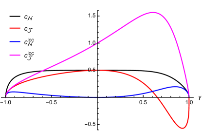
Figure 2: Coefficients (94) in the linear relation (93) between excitation velocities in the Luttinger droplet model  (4) as a function of the interaction parameter $\gamma$ given by (32), (49).

Fig. 2. We note that for $\gamma$ $=$ $0$, the two branches in the Hamiltonian do not mix; in this case $v_{{{\cal N}}}$ and $v_{{{\cal J}}}$ contribute equally to $\bar{v}$ and $\overline{v^{\text{loc}}}$ equals $v_{{{\cal N}}}$. On the other hand, for only interbranch interactions ($\gamma$ $\to$ $\pm 1$), $\bar{\gamma}$ vanishes and hence so do $v_{{{\cal N}},{{\cal J}}}$.

A preliminary physical interpretation of the velocities (92) might be that $\bar{v}$ plays the role of group velocity, as $\bar{v}q$ is the energy of a bosonic excitation in (44) which involves a nonlocal and mixed-flavor superposition of original fermions. On the other hand, since $v^{\text{loc}}(x)$ plays the role of a local phase velocity, its scale is presumably captured by the arithmetic average $\overline{v^{\text{loc}}}$. Note that for the translationally invariant case $\bar{v}$ $=$ $\bar{\gamma}\tilde{v}_{\text{F}}$, and indeed the group velocity and (position-independent) phase velocity are both given by $\bar{v}$, cf. (44), (46), (74).

We conclude that for the Luttinger droplet model (4) the quantities $\bar{v}$, $\overline{v^{\text{loc}}}$, $v_{{{\cal N}}}$, $v_{{{\cal J}}}$, and $\gamma$ are related, extending the Luttinger liquid relations between $\bar{v}$, $v_{{\cal N}}$, $v_{{\cal J}}$, $\gamma$ to the position-dependent case. However, it remains to clarify how the relations (93) evolve away from the special case (4b). Furthermore, in order to be regarded as a paradigm for one-dimensional electronic systems with position-dependent interactions, these relations would have to remain valid also for weak nonlinearites in the dispersion. Both of these questions would therefore be worthwhile to address, e.g., by perturbative methods.

VI Conclusion

Using higher-order bosonization identities, i.e., Kronig-type relations with finite momentum transfer, we solved the Luttinger droplet model (4) for a large class of position-dependent interactions and arbitrary one-particle potentials. While the diagonalized Hamiltonian has the same operator expression as for the Luttinger liquid, the relation between its velocity parameters is not fulfilled in general, as the bosonic excitations and particle number changes involve different averages of the interaction potential over all positions. Similarly the Green functions retain their power-law form for weak position-dependence of the interaction potential, but their exponents also no longer depend only on the ratio of excitation velocities for particle-number changes. For weak position-dependent interactions the Luttinger-liquid characteristics are rather robust regarding their functional form, although the interrelation of the dressed scales and exponents is somewhat different. On the other hand, for an interaction potential with different (e.g., constant) values inside or outside a central region of finite width, not only are the Luttinger-liquid velocity relations modified, but also the Green function is no longer translationally invariant and exhibits a position-dependent propagation velocity of single-particle excitations. This may mean that the group velocity of such an excitation differs from its (position-dependent) phase velocity, in contrast to the Luttinger liquid. We conclude that the Luttinger droplet model has a ground state with different characteristics than the Luttinger liquid. It remains to be seen how the velocity relations obtained for (4) evolve for more general one-dimensional models with position-dependent interactions, and whether a Luttinger droplet paradigm emerges for them.

- (1) D. Sénéchal, arXiv:cond-mat/9908262 .
- Giamarchi (2003) T. Giamarchi, Quantum Physics in One Dimension (Clarendon Press, 2003).
- Tomonaga (1950) S.-I. Tomonaga, Prog. Theor. Phys. 5, 544 (1950).
- Luttinger (1963) J. M. Luttinger, J. Math. Phys. 4, 1154 (1963).
- Mattis and Lieb (1965) D. C. Mattis and E. H. Lieb, J. Math. Phys. 6, 304 (1965).
- Schick (1968) M. Schick, Phys. Rev. 166, 404 (1968).
- Schotte and Schotte (1969) K. D. Schotte and U. Schotte, Phys. Rev. 182, 479 (1969).
- Mattis (1974) D. C. Mattis, J. Math. Phys. 15, 609 (1974).
- Luther and Peschel (1974) A. Luther and I. Peschel, Phys. Rev. B 9, 2911 (1974).
- Coleman (1975) S. Coleman, Phys. Rev. D 11, 2088 (1975).
- Mandelstam (1975) S. Mandelstam, Phys. Rev. D 11, 3026 (1975).
- Heidenreich et al. (1975) R. Heidenreich, B. Schroer, R. Seiler, and D. Uhlenbrock, Phys. Lett. A 54, 119 (1975).
- Haldane (1979) F. D. M. Haldane, J. Phys. C: Solid State Phys. 12, 4791 (1979).
- Haldane (1981a) F. D. M. Haldane, J. Phys. C: Solid State Phys. 14, 2585 (1981a).
- Emery (1979) V. J. Emery, in Highly Conducting One-Dimensional Solids, Physics of Solids and Liquids, edited by J. T. Devreese, R. P. Evrard, and V. E. v. Doren (Springer, 1979) p. 247.
- Voit (1995) J. Voit, Rep. Prog. Phys. 58, 977 (1995).
- Kotliar and Si (1996) G. Kotliar and Q. Si, Phys. Rev. B 53, 12373 (1996).
- von Delft and Schoeller (1998) J. von Delft and H. Schoeller, Ann. Phys. 7, 225 (1998).
- von Delft et al. (1998) J. von Delft, G. Zaránd, and M. Fabrizio, Phys. Rev. Lett. 81, 196 (1998).
- Zaránd and von Delft (2000) G. Zaránd and J. von Delft, Phys. Rev. B 61, 6918 (2000).
- Lee and Chen (1988) D. K. K. Lee and Y. Chen, J. Phys. A: Math. Gen. 21, 4155 (1988).
- Yurkevich (2002) I. V. Yurkevich, in Strongly Correlated Fermions and Bosons in Low-Dimensional Disordered Systems, NATO Science Series (Springer, Dordrecht, 2002) pp. 69–80.
- Grishin et al. (2004) A. Grishin, I. V. Yurkevich, and I. V. Lerner, Phys. Rev. B 69, 165108 (2004).
- Galda et al. (2011) A. Galda, I. V. Yurkevich, and I. V. Lerner, Phys. Rev. B 83, 041106 (2011).
- Filippone and Brouwer (2016) M. Filippone and P. W. Brouwer, Phys. Rev. B 94, 235426 (2016).
- Meden and Schönhammer (1992) V. Meden and K. Schönhammer, Phys. Rev. B 46, 15753 (1992).
- Schönhammer and Meden (1993a) K. Schönhammer and V. Meden, Phys. Rev. B 47, 16205 (1993a).
- Schönhammer and Meden (1993b) K. Schönhammer and V. Meden, Phys. Rev. B 48, 11521 (1993b).
- Meden (1999) V. Meden, Phys. Rev. B 60, 4571 (1999).
- Markhof and Meden (2016) L. Markhof and V. Meden, Phys. Rev. B 93, 085108 (2016).
- Haldane (1980) F. D. M. Haldane, Phys. Rev. Lett. 45, 1358 (1980).
- Haldane (1981b) F. D. M. Haldane, Phys. Lett. A 81, 153 (1981b).
- Haldane (1981c) F. D. M. Haldane, Phys. Rev. Lett. 47, 1840 (1981c).
- Sólyom (1979) J. Sólyom, Adv. Phys. 28, 201 (1979).
- (35) K. Schönhammer, arXiv:cond-mat/9710330 .
- Schönhammer (2004) K. Schönhammer, in Strong interactions in low dimensions, Physics and Chemistry of Materials with Low-Dimensional Structures, edited by D. Baeriswyl and L. Degiorgi (Springer Netherlands, 2004) p. 93.
- Schönhammer (2013) K. Schönhammer, J. Phys.: Condens. Matter 25, 014001 (2013).
- Miranda (2003) E. Miranda, Braz. J. Phys. 33, 3 (2003).
- Cazalilla et al. (2011) M. A. Cazalilla, R. Citro, T. Giamarchi, E. Orignac, and M. Rigol, Rev. Mod. Phys. 83, 1405 (2011).
- Kopietz (1997) P. Kopietz, Bosonization of Interacting Fermions in Arbitrary Dimensions (Springer, 1997).
- Gogolin et al. (2004) A. O. Gogolin, A. A. Nersesyan, and Alexei M. Tsvelik, Bosonization and Strongly Correlated Systems (Cambridge University Press, 2004).
- Bruus and Flensberg (2004) H. Bruus and K. Flensberg, Many-Body Quantum Theory in Condensed Matter Physics: An Introduction (Oxford University Press, 2004).
- Giuliani and Vignale (2008) G. Giuliani and G. Vignale, Quantum Theory of the Electron Liquid (Cambridge University Press, 2008).
- Phillips (2012) P. Phillips, Advanced Solid State Physics, 2nd ed. (Cambridge University Press, 2012).
- Mastropietro and Mattis (2013) V. Mastropietro and D. C. Mattis, Luttinger Model - The First 50 Years and Some New Directions, Series on Directions in Condensed Matter Physics, Vol. 20 (World Scientific, 2013).
- Milliken et al. (1996) F. P. Milliken, C. P. Umbach, and R. A. Webb, Sol. State Comm. 97, 309 (1996).
- Maasilta and Goldman (1997) I. J. Maasilta and V. J. Goldman, Phys. Rev. B 55, 4081 (1997).
- Chang (2003) A. M. Chang, Rev. Mod. Phys. 75, 1449 (2003).
- Bockrath et al. (1999) M. Bockrath, D. H. Cobden, J. Lu, A. G. Rinzler, R. E. Smalley, L. Balents, and P. L. McEuen, Nature 397, 598 (1999).
- Ishii et al. (2003) H. Ishii, H. Kataura, H. Shiozawa, H. Yoshioka, H. Otsubo, Y. Takayama, T. Miyahara, S. Suzuki, Y. Achiba, M. Nakatake, T. Narimura, M. Higashiguchi, K. Shimada, H. Namatame, and M. Taniguchi, Nature 426, 540 (2003).
- Aleshin et al. (2004) A. N. Aleshin, H. J. Lee, Y. W. Park, and K. Akagi, Phys. Rev. Lett. 93, 196601 (2004).
- Boninsegni et al. (2007) M. Boninsegni, A. B. Kuklov, L. Pollet, N. V. Prokof’ev, B. V. Svistunov, and M. Troyer, Phys. Rev. Lett. 99, 035301 (2007).
- Del Maestro et al. (2011) A. Del Maestro, M. Boninsegni, and I. Affleck, Phys. Rev. Lett. 106, 105303 (2011).
- Duc et al. (2015) P.-F. Duc, M. Savard, M. Petrescu, B. Rosenow, A. D. Maestro, and G. Gervais, Science Advances 1, e1400222 (2015).
- Jompol et al. (2009) Y. Jompol, C. J. B. Ford, J. P. Griffiths, I. Farrer, G. A. C. Jones, D. Anderson, D. A. Ritchie, T. W. Silk, and A. J. Schofield, Science 325, 597 (2009).
- Barak et al. (2010) G. Barak, H. Steinberg, L. N. Pfeiffer, K. W. West, L. Glazman, F. von Oppen, and A. Yacoby, Nat. Phys. 6, 489 (2010).
- Blumenstein et al. (2011) C. Blumenstein, J. Schäfer, S. Mietke, S. Meyer, A. Dollinger, M. Lochner, X. Y. Cui, L. Patthey, R. Matzdorf, and R. Claessen, Nat. Phys. 7, 776 (2011).
- Mebrahtu et al. (2012) H. T. Mebrahtu, I. V. Borzenets, D. E. Liu, H. Zheng, Y. V. Bomze, A. I. Smirnov, H. U. Baranger, and G. Finkelstein, Nature 488, 61 (2012).
- Mebrahtu et al. (2013) H. T. Mebrahtu, I. V. Borzenets, H. Zheng, Y. V. Bomze, A. I. Smirnov, S. Florens, H. U. Baranger, and G. Finkelstein, Nature Physics 9, 732 (2013).
- Yang et al. (2017) B. Yang, Y.-Y. Chen, Y.-G. Zheng, H. Sun, H.-N. Dai, X.-W. Guan, Z.-S. Yuan, and J.-W. Pan, Phys. Rev. Lett. 119, 165701 (2017).
- Cedergren et al. (2017) K. Cedergren, R. Ackroyd, S. Kafanov, N. Vogt, A. Shnirman, and T. Duty, Phys. Rev. Lett. 119, 167701 (2017).
- (62) R. Stühler, F. Reis, T. Müller, T. Helbig, T. Schwemmer, R. Thomale, J. Schäfer, and R. Claessen, arXiv:1901.06170 .
- Busche and Kopietz (2000) T. Busche and P. Kopietz, Int. J. Mod. Phys. B 14, 1481 (2000).
- Pirooznia et al. (2008) P. Pirooznia, F. Schütz, and P. Kopietz, Phys. Rev. B 78, 075111 (2008).
- Teber (2007) S. Teber, Phys. Rev. B 76, 045309 (2007).
- Karrasch et al. (2015) C. Karrasch, R. G. Pereira, and J. Sirker, New J. Phys. 17, 103003 (2015).
- Rozhkov (2003) A. V. Rozhkov, Phys. Rev. B 68, 115108 (2003).
- Rozhkov (2005) A. V. Rozhkov, Eur. Phys. J. B 47, 193 (2005).
- Rozhkov (2006) A. V. Rozhkov, Phys. Rev. B 74, 245123 (2006).
- Rozhkov (2008) A. V. Rozhkov, Phys. Rev. B 77, 125109 (2008).
- Rozhkov (2014) A. V. Rozhkov, Phys. Rev. Lett. 112, 106403 (2014).
- Imambekov and Glazman (2009a) A. Imambekov and L. I. Glazman, Science 323, 228 (2009a).
- Imambekov and Glazman (2009b) A. Imambekov and L. I. Glazman, Phys. Rev. Lett. 102, 126405 (2009b).
- Imambekov et al. (2012) A. Imambekov, T. L. Schmidt, and L. I. Glazman, Rev. Mod. Phys. 84, 1253 (2012).
- Maebashi and Takada (2014) H. Maebashi and Y. Takada, Phys. Rev. B 89, 201109 (2014).
- Essler et al. (2015) F. H. L. Essler, R. G. Pereira, and I. Schneider, Phys. Rev. B 91, 245150 (2015).
- Markhof et al. (2019) L. Markhof, M. Pletyukov, and V. Meden, SciPost Physics 7, 047 (2019).
- Cazalilla (2006) M. A. Cazalilla, Phys. Rev. Lett. 97, 156403 (2006).
- Iucci and Cazalilla (2009) A. Iucci and M. A. Cazalilla, Phys. Rev. A 80, 063619 (2009).
- Nessi and Iucci (2013) N. Nessi and A. Iucci, Phys. Rev. B 87, 085137 (2013).
- Uhrig (2009) G. S. Uhrig, Phys. Rev. A 80, 061602 (2009).
- Foster et al. (2010) M. S. Foster, E. A. Yuzbashyan, and B. L. Altshuler, Phys. Rev. Lett. 105, 135701 (2010).
- Perfetto and Stefanucci (2011) E. Perfetto and G. Stefanucci, EPL 95, 10006 (2011).
- Dziarmaga and Tylutki (2011) J. Dziarmaga and M. Tylutki, Phys. Rev. B 84, 214522 (2011).
- Dóra et al. (2011) B. Dóra, M. Haque, and G. Zaránd, Phys. Rev. Lett. 106, 156406 (2011).
- Dóra et al. (2012) B. Dóra, Á. Bácsi, and G. Zaránd, Phys. Rev. B 86, 161109 (2012).
- Dóra and Pollmann (2015) B. Dóra and F. Pollmann, Phys. Rev. Lett. 115, 096403 (2015).
- Dóra et al. (2016) B. Dóra, R. Lundgren, M. Selover, and F. Pollmann, Phys. Rev. Lett. 117, 010603 (2016).
- Karrasch et al. (2012) C. Karrasch, J. Rentrop, D. Schuricht, and V. Meden, Phys. Rev. Lett. 109, 126406 (2012).
- Rentrop et al. (2012) J. Rentrop, D. Schuricht, and V. Meden, New J. Phys. 14, 075001 (2012).
- Coira et al. (2013) E. Coira, F. Becca, and A. Parola, Eur. Phys. J. B 86, 1 (2013).
- Ngo Dinh et al. (2013) S. Ngo Dinh, D. A. Bagrets, and A. D. Mirlin, Phys. Rev. B 88, 245405 (2013).
- Sabetta and Misguich (2013) T. Sabetta and G. Misguich, Phys. Rev. B 88, 245114 (2013).
- Kennes and Meden (2013) D. M. Kennes and V. Meden, Phys. Rev. B 88, 165131 (2013).
- Kennes et al. (2014) D. M. Kennes, C. Klöckner, and V. Meden, Phys. Rev. Lett. 113, 116401 (2014).
- Sachdeva et al. (2014) R. Sachdeva, T. Nag, A. Agarwal, and A. Dutta, Phys. Rev. B 90, 045421 (2014).
- Schiró and Mitra (2015) M. Schiró and A. Mitra, Phys. Rev. B 91, 235126 (2015).
- Mastropietro and Wang (2015) V. Mastropietro and Z. Wang, Phys. Rev. B 91, 085123 (2015).
- Gutman et al. (2010) D. B. Gutman, Y. Gefen, and A. D. Mirlin, Phys. Rev. B 81, 085436 (2010).
- Protopopov et al. (2011) I. V. Protopopov, D. B. Gutman, and A. D. Mirlin, J. Stat. Mech. 2011, P11001 (2011).
- Protopopov et al. (2014a) I. V. Protopopov, D. B. Gutman, and A. D. Mirlin, Phys. Rev. B 90, 125113 (2014a).
- Protopopov et al. (2014b) I. V. Protopopov, D. B. Gutman, M. Oldenburg, and A. D. Mirlin, Phys. Rev. B 89, 161104 (2014b).
- Protopopov et al. (2015) I. V. Protopopov, D. B. Gutman, and A. D. Mirlin, Phys. Rev. B 91, 195110 (2015).
- Lin et al. (2013) J. Lin, K. A. Matveev, and M. Pustilnik, Phys. Rev. Lett. 110, 016401 (2013).
- Buchhold and Diehl (2015a) M. Buchhold and S. Diehl, Phys. Rev. A 92, 013603 (2015a).
- Buchhold and Diehl (2015b) M. Buchhold and S. Diehl, Eur. Phys. J. D 69, 1 (2015b).
- Buchhold et al. (2016) M. Buchhold, M. Heyl, and S. Diehl, Phys. Rev. A 94, 013601 (2016).
- Huber et al. (2018) S. Huber, M. Buchhold, J. Schmiedmayer, and S. Diehl, Phys. Rev. A 97, 043611 (2018).
- Kronig (1935) R. D. Kronig, Physica 2, 968 (1935).
- Dover (1968) C. B. Dover, Ann. Phys. 50, 500 (1968).
- Note (1) Throughout, hats appear only on those operators which involve fermionic number operators.
- Kane and Fisher (1992a) C. L. Kane and M. P. A. Fisher, Phys. Rev. Lett. 68, 1220 (1992a).
- Kane and Fisher (1992b) C. L. Kane and M. P. A. Fisher, Phys. Rev. B 46, 15233 (1992b).
- Kane and Fisher (1992c) C. L. Kane and M. P. A. Fisher, Phys. Rev. B 46, 7268 (1992c).
- Rylands and Andrei (2016) C. Rylands and N. Andrei, Phys. Rev. B 94, 115142 (2016).
- Rylands and Andrei (2017) C. Rylands and N. Andrei, Phys. Rev. B 96, 115424 (2017).
- Rylands and Andrei (2018) C. Rylands and N. Andrei, Phys. Rev. B 97, 155426 (2018).
- Meden et al. (2002) V. Meden, W. Metzner, U. Schollwöck, and K. Schönhammer, J. Low Temp. Phys. 126, 1147 (2002).
- Hattori and Rosch (2014) K. Hattori and A. Rosch, Phys. Rev. B 90, 115103 (2014).
- Meden et al. (2000) V. Meden, W. Metzner, U. Schollwöck, O. Schneider, T. Stauber, and K. Schönhammer, Eur. Phys. J. B 16, 631 (2000).
- Schneider and Eggert (2010) I. Schneider and S. Eggert, Phys. Rev. Lett. 104, 036402 (2010).
- (122) C. Rylands, arXiv:1910.11221 .
- Eggert (2000) S. Eggert, Phys. Rev. Lett. 84, 4413 (2000).
- Wonneberger (2001) W. Wonneberger, Phys. Rev. A 63, 063607 (2001).
- Maslov and Stone (1995) D. L. Maslov and M. Stone, Phys. Rev. B 52, R5539 (1995).
- Safi and Schulz (1995) I. Safi and H. J. Schulz, Phys. Rev. B 52, R17040 (1995).
- Ponomarenko (1995) V. V. Ponomarenko, Phys. Rev. B 52, R8666 (1995).
- Rech and Matveev (2008a) J. Rech and K. A. Matveev, J. Phys.: Condens. Matter 20, 164211 (2008a).
- Rech and Matveev (2008b) J. Rech and K. A. Matveev, Phys. Rev. Lett. 100, 066407 (2008b).
- Ferrier-Barbut (2019) I. Ferrier-Barbut, Physics Today 72, 46 (2019).
- Note (2) We note that our derivation of (7\@@italiccorr) is similar in spirit to the procedure in Sec. 3.2 of Ref. \rev@citealpnumpereira_dynamical_2007, and also bears some resemblance to the analysis of higher-order dispersion terms in Ref. \rev@citealpnumenciso_fermion_2006,*karabali_exact_2014. However our approach is more general since we also allow finite momentum transfer and work with exact operator identities. Note also that one may view (7\@@italiccorr) as a fermionic representation of certain properties of vertex operators,von Delft and Schoeller (1998) i.e., exponentiated bosonic fields.
- Pereira et al. (2007) R. G. Pereira, J. Sirker, J.-S. Caux, R. Hagemans, J. M. Maillet, S. R. White, and I. Affleck, J. Stat. Mech. 2007, P08022 (2007).
- Enciso and Polychronakos (2006) A. Enciso and A. P. Polychronakos, Nucl. Phys. B 751, 376 (2006).
- Karabali and Polychronakos (2014) D. Karabali and A. P. Polychronakos, Phys. Rev. D 90, 025002 (2014).
- Francesco et al. (1997) P. D. Francesco, P. Mathieu, and D. Sénéchal, Conformal Field Theory (Springer, 1997).
- Comtet (1974) L. Comtet, Advanced Combinatorics (Springer Netherlands, Dordrecht, 1974).