Magnetic Field Effect on Dynamics of Entanglement
for Time-dependent Harmonic Oscillator

Radouan Hab-arrih ^a, Ahmed Jellal^a,b and Abdeldjalil Merdaci^b

^aLaboratory of Theoretical Physics, Faculty of Sciences, Chouaïb Doukkali University,

PO Box 20, 24000 El Jadida, Morocco

^bCanadian Quantum Research Center, 204-3002 32 Ave Vernon,
BC V1T 2L7, Canada

^cDepartment of Physics, Faculty of Sciences, University of 20 août 1955-Skikda,
Road El-Hadaeik, B.P. 26, 21000, Skikda, Algeria

We investigate the dynamics of entanglement, uncertainty and mixedness by solving time dependent Schrödinger equation for two-dimensional harmonic oscillator with time dependent frequency and coupling parameter subject to a static magnetic field. We compute the purities (global/marginal) and then calculate explicitly the linear entropy $S_{L}$ as well as logarithmic negativity $\mathcal{N}$ using the symplectic parametrization of vacuum state. We introduce the spectral decomposition to diagonalize the marginal state and get the expression of von Neumann entropy $S_{von}$ and establish its link with $S_{L}$. We use the Wigner formalism to derive the Heisenberg uncertainties and show their dependencies on both $S_{L}$ and the coupling parameters $\gamma_{i}$ $(i=1,2)$ of the quadrature term $x_{i}p_{i}$. We graphically study the dynamics of the three features (entanglement, uncertainty, mixedness) and present the similar topology with respect to time. We show the effects of the magnetic field and quenched values of $J(t)$ and $\omega_{2}(t)$ on these three dynamics, which lead eventually to control and handle them.

PACS numbers: 03.65.Fd, 03.65.Ge, 03.65.Ud, 03.67.Hk
Keywords: Time-dependent harmonic oscillator, magnetic field, entanglement, logarithmic negativity, quenched model, uncertainty.

1 Introduction

The entanglement, uncertainty and mixedness are three fundamental and remarkably features of the quantum information. Indeed firstly, the entanglement is the most amazing property of quantum mechanics, which expresses the ”spooky” non-locality action [1] between quantum states but it is still a physical reality [2]. With the entanglement one can describe a large type of physical phenomena and related issues [3]. The von Neumann entropy [1] of the reduced states or generally the Rényi entropies [4, 5] can be used as suitable quantifiers of entanglement amount for pure bipartite states (i.e. $\mathcal{H}=\mathcal{H}_{A}\otimes\mathcal{H}_{B}$). However, for mixed states the quantification of non-local correlations is still an open problem [1, 6]. This is due to the fact that there exist infinitely many pure state decomposition, which complicate such quantification. Secondly, the uncertainty lies at the core of quantum physics and presents a key of the discrepancies between classical and quantum systems [7]. It can be understood mathematically as two observables, which are conjugate (i.e. connected by the Fourier transform) and the trade-off between their spreads can not be zero. In the early twentieth century, Heisenberg proposed in a seminal paper [8] showing the variance-based uncertainty for position and momentum $\Delta x\Delta p\geq\frac{\hslash}{2}$. This has been extended to generalized uncertainties, one of them is the Robertson-Schrödinger uncertainty $\Delta_{A}\Delta_{B}\geq\frac{1}{2}\left[|\langle\{A,B\}\rangle-2\langle A\rangle\langle B\rangle|^{2}+|\langle\left[A,B\right]\rangle|^{2}\right]^{\frac{1}{2}}$, with $A$ and $B$ are two arbitrary observables, while the averages are with respect to the quantum state $|{\Psi}\rangle$ encoding those fluctuations [9]. Recently more general uncertainties based on entropy were introduced to be used as entanglement witnesses [10, 8]. Thirdly, the mixedness is the loss of information caused by the preparation of states. Consequently, the mixed state can be written as a convex linear combination of pure states $|{\Psi}\rangle=\sum_{i=1}^{n}p_{i}|\phi_{i}\rangle$ with the conservation of the quantum probabilities, i.e. $\sum_{i=1}^{n}p_{i}=1$. It is worthwhile noting that $(p_{i})_{i=1,\cdots,n}$ are classical probabilistic distributions, which is the point that distinguish the mixedness and superposition principle. We mention that different studies showed that the three fundamental features, mentioned above, are related [4, 11, 12].

The study of problems addressing to the coupled harmonic oscillators with time dependent frequencies has of paramount importance in different scientific branches. This is due to its intrinsic mathematical interest and its power to model the behavior of systems in the vicinity of their equilibrium. Their time dependent Schrödinger equation (TDSE) was solved exactly using different methods [13, 14, 15, 16]. The solutions of TDSE were widely used to investigate the dynamics of entanglement [4, 3] and uncertainty [4] for bipartite systems. Many works dealt with the Gaussian solutions (e.g. vacuum [4, 3], thermal [5], squeezed [11], coherent $\cdots$) and have been considered as prototypical continuum variables. This is quite natural because they can be created and assisted via linear optics. Recently, it was shown that the entanglement can be assisted via temperature [5], magnetic field [17] and both [18], but most of works dealt with time independent potential.

We study the effect of magnetic field on the dynamics of entanglement for two-dimensional harmonic oscillator with time-dependent frequency and coupling parameter. We embark on the vacuum state and determine the purity function, which allows us to quantify the entanglement together with the degree of mixedness and quantum fluctuations. We show that the magnetic field purifies the marginal states in decreasing the amount of quantum fluctuations and small values of the quenched frequencies increase them. In addition, using the Wigner function we derive the uncertainty relations in terms of the linear entropy telling us that its lower bound depends on magnetic field and time. This is important feature to preserve the invariance of uncertainty relations with respect to phase space transformations during the action of magnetic field and dynamics.

The present paper is organized as follows. In section 2, we reduce the Hamiltonian into a diagonalized form using some transformations. In section 3, we solve the associated TDSE and cast the eigen-spectrum of the time-dependent harmonic oscillator expressed with respect to original phase space coordinates. In section 4, we compute the global and marginal purities, which will be used to discuss the mixedness via linear entropy $S_{L}$. Then we obtain the decomposition of the marginal state $\rho^{A}_{(0,0)}$ that leading to compute the von Neumann entropy $S_{von}$. In section 5, we study the dynamics of entanglement via logarithmic negativity $\mathcal{N}$ and discuss its relationship to $S_{L}$. In section 6, we calculate the fluctuations encoded in the vacuum state using the Heisenberg uncertainty and discuss some limiting cases. In section 7, we involve a realistic quenched model to follow the dynamics and study the effects of magnetic field, quenched coupling $J_{f}$ and frequency $\omega_{2,f}$ on the dynamics of entanglement, uncertainty and mixedness. Finally, we summarize our results.

2 Diagonalized Hamiltonian

The machinery of the coupled harmonic oscillators is successfully used to investigate the effect of the rest of universe on the entropy and quantum fluctuations [19], the Bogoliubov transformation model of superconductivity [20], the magnetoresistance [21], the cyclotron resonance [22] and so on. The time-dependent harmonic oscillator has received much attention because of its applications in several areas of physics [23], since the variable-mass and variable-frequency oscillators are important in quantum optics as well as in many other fields. As for the time-dependent coupled harmonic oscillators, they are the best candidate to describe several quantum mechanical problems. Among them, we cite the ion-laser interactions [24], quantized fields propagating through dielectric media [25], shortcuts to adiabaticity [26, 27], the Casimir effect [28, 29]. They can be used as a toy model to study aspects of the final stages of black-hole evaporation [30] and their Schmidt modes in the study of quantum entanglement [31].

Motivated by the above achievements, we consider a charged particle in magnetic field described by a two-dimensional harmonic oscillator with time-dependent frequency and coupling parameter in the presence of a static perpendicular magnetic field. In this case, the canonical momenta $\vec{p}=(p_{1},p_{2})$ will be replaced by the conjugate momenta $(\pi_{1},\pi_{2})=\vec{p}-\frac{e}{c}\vec{A}$ where $\vec{A}$ is the potential vector such that $\vec{\nabla}\wedge\vec{A}=\vec{B}$. The corresponding Hamiltonian is

$$H_{0}=\frac{1}{2}\left(\pi_{1}^{2}+\pi_{2}^{2}\right)+\frac{1}{2}\omega_{1}^{2}(t)x_{1}^{2}+\frac{1}{2}\omega_{2}^{2}(t)x_{2}^{2}-J(t)x_{1}x_{2}$$ (1)

where the frequencies $\omega_{i}(t)$ ($i=1,2$) and coupling $J(t)>0$ are three parameters time-dependent. To proceed further, we choose the symmetric gauge $\vec{A}=\frac{B}{2}(x_{2},-x_{1})$ to obtain the conjugate momenta

$$\pi_{1}=p_{1}+\dfrac{eB}{2c}x_{2},\qquad\pi_{2}=p_{2}-\dfrac{eB}{2c}x_{1}$$ (2)

which can be substituted into $H_{0}$ to get

$$H_{1}=\dfrac{p_{1}^{2}+p_{2}^{2}}{2}+\frac{1}{2}\Omega_{1}^{2}(t)x_{1}^{2}+\frac{1}{2}\Omega_{2}^{2}(t)x_{2}^{2}-J(t)x_{1}x_{2}+\omega_{c}\left(p_{1}x_{2}-p_{2}x_{1}\right)$$ (3)

where we have set $\Omega_{i}^{2}(t)=\omega_{i}^{2}(t)+\omega_{c}^{2}$ and $\omega_{c}=\dfrac{eB}{2c}$ is the cyclotron frequency. It is clearly seen that our system is now described by two coupled harmonic oscillators together with the angular momentum operator $L_{z}$. We will study the quantum information of the time-dependent coupled harmonic oscillators by showing that $B$ plays a crucial role in the dynamics of entanglement encoded in the both continuum variable quantifiers von Neumann entropy $S_{von}$ and logarithmic negativity $E_{\mathcal{N}}$. This fact will due to strong dependence of the solutions $h_{i}(t,\omega_{c})$ (equations (81-82)) of Ermakov equation on the frequency $\omega_{c}$, which undergo important amplitudes and frequency modulations with respect to $\omega_{c}$. Note in passing that the Hamiltonian (1) was previously established in the literature to study different issues. For instance, it is introduced to resolve the both dynamics (quantum/classical) using two different approaches (unitary transformation/generating function) and considering time-dependent quantities (mass, frequencies, magnetic field and coupling parameter) [32].

To get rid of the operator $L_{z}$, we introduce a quantum canonical transformation from $\left(x_{1},x_{2},p_{1},p_{2}\right)$ to new variables $\left(y_{1},y_{2},P_{1},P_{2}\right)$. This is

$$\left(\begin{matrix}x_{1}\\ x_{2}\end{matrix}\right)=\left(\begin{matrix}\cos\phi\left(t\right)&\sin\phi\left(t\right)\\ -\sin\phi\left(t\right)&\cos\phi\left(t\right)\end{matrix}\right)\allowbreak\left(\begin{matrix}y_{1}\\ y_{2}\end{matrix}\right),\qquad\left(\begin{matrix}p_{1}\\ p_{2}\end{matrix}\right)=\left(\begin{matrix}\cos\phi\left(t\right)&\sin\phi\left(t\right)\\ -\sin\phi\left(t\right)&\cos\phi\left(t\right)\end{matrix}\right)\allowbreak\left(\begin{matrix}P_{1}\\ P_{2}\end{matrix}\right)$$ (4)

and we have [33]

$$p_{1} =\frac{\partial\hat{F}_{2}\left(x_{1},x_{2},P_{1},P_{2};t\right)}{\partial x_{1}},\qquad p_{2}=\frac{\partial\hat{F}_{2}\left(x_{1},x_{2},P_{1},P_{2};t\right)}{\partial x_{2}}$$ (5)

$$y_{1} =\frac{\partial\hat{F}_{2}\left(x_{1},x_{2},P_{1},P_{2};t\right)}{\partial P_{1}},\qquad y_{2}=\frac{\partial\hat{F}_{2}\left(x_{1},x_{2},P_{1},P_{2};t\right)}{\partial P_{2}}$$ (6)

where the hermitian generating function is given by

$$\hat{F}_{2}\left(x_{1},x_{2},P_{1},P_{2};t\right)=\frac{P_{1}x_{1}+x_{1}P_{1}+P_{2}x_{2}+x_{2}P_{2}}{2}\cos\phi\left(t\right)+\left(P_{2}x_{1}-P_{1}x_{2}\right)\sin\phi\left(t\right)$$ (7)

showing that

$$\frac{\partial}{\partial t}\hat{F}_{2}\left(x_{1},x_{2},P_{1},P_{2};t\right)=\dot{\phi}\left(t\right)\left(-P_{1}y_{2}+P_{2}y_{1}\right).$$ (8)

According to [33, 34], the above quantum function can be used to express the Hamiltonian into the new coordinate representation as

$$H_{2}=H_{1}+\frac{\partial\hat{F}_{2}\left(x_{1},x_{2},P_{1},P_{2};t\right)}{\partial t}=H_{1}-\dot{\phi}\left(t\right)\left(P_{1}y_{2}-P_{2}y_{1}\right).$$ (9)

It worthwhile to mention that the method of canonical transformations (CT) and generating function (GF) proved to be a fruitful approach in treating quantum systems. Recall that two systems described by the Hamiltonian’s $H_{0}$ and $H_{1}$ are canonically equivalent if they are related by a canonical or equivalently unitary operation, which conserves all the quantum eigen-spectrum and the mean values of observables. The mapping $(\vec{\pi},x)\mapsto(\vec{p},x)$ is not a CT (i.e $[\pi_{1},\pi_{2}]=2i\omega_{c}$) but just a substitution and we do not have any transformation on position representation $(x_{1},x_{2})$, then the transformation does not affect the Hamiltonian function $H_{0}(x_{1},x_{2},t)=H_{1}(x_{1},x_{2},t)$. In the generating function theory [33], a generating function $F$ exists and then the Hamiltonian must verifies the condition $H_{1}(x_{1},x_{2})=H_{0}(x_{1},x_{2})+\frac{\partial F}{\partial t}$, obviously $\frac{\partial F}{\partial t}=0$ for time-independent systems, more clarification can be found in [33]. Now, imposing the condition $\dot{\phi}\left(t\right)=\omega_{c}$ we obtain a linear equation in time

$$\phi\left(t\right)=\omega_{c}t+\theta$$ (10)

and the angle $\theta$ is a constant of integration. In this case, $H_{2}$ becomes

$$H_{2}=\frac{1}{2}\left(P_{1}^{2}+P_{2}^{2}\right)+\frac{1}{2}\sigma_{1}^{2}(t,B)y_{1}^{2}+\frac{1}{2}\sigma_{2}^{2}(t,B)y_{2}^{2}+\sigma_{3}(t,B)y_{1}y_{2}$$ (11)

with $\sigma_{j}^{2}=\varsigma^{2}_{j}+\omega_{c}^{2}$ $(j=1,2)$ and

$$\varsigma_{1}^{2}(t,B) =\omega_{1}^{2}(t)\cos^{2}\phi(t)+\omega_{2}^{2}(t)\sin^{2}\phi(t)+J(t)\sin 2\phi(t)$$ (12)

$$\varsigma_{2}^{2}(t,B) =\omega_{1}^{2}(t)\sin^{2}\phi(t)+\omega_{2}^{2}(t)\cos^{2}\phi(t)-J(t)\sin 2\phi(t)$$ (13)

$$\sigma_{3}(t,B) =\tfrac{\omega_{1}^{2}(t)-\omega_{2}^{2}(t)}{2}\sin 2\phi(t)-J(t)\cos 2\phi(t).$$ (14)

At this stage, let us look for the appropriate rotation of angle $\phi(t)$ that leads to the uncoupled harmonic oscillators. To this end, we use a method extremely employed in different context to deal with many issues. For instance by selecting the appropriate rotation, Han et al. [35] showed that the coupled harmonic oscillator can be diagonalized and would yield an increased entropy in the observable oscillator, providing a clarification of Feynman’s rest of the universe. Subsequently, the same technique has been used in generalizing the Han et al. [35] work to the non-commutative space [36], studying the entanglement of coupled harmonic oscillators [37, 4, 38, 39] and proposing an alternative approach to exact wave functions for time-dependent coupled oscillator model of charged particle in variable magnetic field [32]. Similarly, we can choose the rotation

$$\tan 2\phi(t)=\frac{2J(t)}{\omega_{1}^{2}(t)-\omega_{2}^{2}(t)}$$ (15)

to ensures the solvability of the Hamiltonian describing our system. We emphasis that (15) is a necessary and sufficient condition (NSC), which holds for all time and corresponds to $\sigma_{3}(t,B)=0$ in (14). Since it depends only on the original parameters of the problem $(\omega_{i}(t),J(t))$ then NSC leads directly to an uncoupled Hamiltonian (11) in the $(y_{1},y_{2})$-representation. In our knowledge, this is the unique way to get a diagonalized Hamiltonian and therefore derive the solutions of the energy spectrum. Now, we have some remarks in order. Firstly, (15) is actually connecting the magnetic field $B$ to frequencies $\omega_{i}(t)$ and coupling parameter $J(t)$. Secondly, if the coupling parameter $J(t)$ is switched off then there is no rotation meaning that $\phi(t)=0$ and automatically both $B=0$ and $\theta$ are null. Thirdly for zero time, we recover the rotation with an angle used previously in literature [35, 36, 37], which is

$$\tan 2\theta=\frac{2J(0)}{\omega_{1}^{2}(0)-\omega_{2}^{2}(0)}.$$ (16)

Consequently, the Hamiltonian becomes diagonal

$$H_{2}=\frac{1}{2}\left(P_{1}^{2}+P_{2}^{2}\right)+\frac{1}{2}\sigma_{1}^{2}(t,B)y_{1}^{2}+\frac{1}{2}\sigma_{2}^{2}(t,B)y_{2}^{2}$$ (17)

which will be solved to determine the eigenvalues and eigenfunctions using some techniques involving time dependent frequencies.

3 Exact wavefunctions

We recall that the time dependent Schrödinger equation (TDSE) for any single harmonic oscillator having a frequency time-dependent can be written as

$$-\frac{1}{2}\left[\frac{\partial^{2}}{\partial y_{1}^{2}}-\sigma_{1}^{2}(t,B)y_{1}^{2}\right]\Psi(y_{1},t)=i\frac{\partial\Psi}{\partial t}$$ (18)

that can be exactly solved [15] using theory of invariants [13, 14] or transformation group techniques [16]. The solutions are

$$\Psi_{n}\left(y_{1},t\right)=e^{-i\int_{0}^{t}E_{n}\frac{dt^{\prime}}{h_{1}^{2}(t^{\prime})}}e^{\frac{i}{2}\left(\frac{\dot{h}_{1}}{h_{1}}\right)y_{1}^{2}}\Phi_{n}\left(\frac{y_{1}}{h_{1}}\right),\qquad n\in\mathbb{N}$$ (19)

such that the eigenstates $\Phi_{n}$ and eigenvalues $E_{n}$ are given by

$$\Phi_{n}\left(\frac{y_{1}}{h_{1}}\right)=\dfrac{1}{\sqrt{2^{n}n!}}\left(\dfrac{\tilde{\sigma}_{1}(t,B)}{\pi}\right)^{\frac{1}{4}}H_{n}\left(\sqrt{\tilde{\sigma}_{1}(t,B)}y_{1}\right)e^{\frac{-\tilde{\sigma}_{1}(t,B)}{2}y_{1}^{2}}$$ (20)

$$E_{n}=\sigma_{1}(0,B)\left(n+\frac{1}{2}\right)$$ (21)

where $H_{n}(\epsilon)$ are Hermite polynomials, $\tilde{\sigma}_{1}(t,B)=\frac{\sigma_{1}(0,B)}{h_{1}^{2}(t)}$ with the function $h_{1}(t)$ satisfies the Ermakov equation

$$\ddot{h}_{1}+\sigma_{1}^{2}(t,B)h_{1}=\dfrac{\sigma_{1}^{2}(0,B)}{h_{1}^{3}}$$ (22)

and two initial conditions $h_{1}(0)=1$, $\dot{h}_{1}(0)=0$. Therefore, the wavefunctions associated to the Hamiltonian (17) are

$$\Psi_{n,m}(y_{1},y_{2}:t) = \dfrac{1}{\sqrt{2^{n+m}n!m!}}\left(\dfrac{\tilde{\sigma}_{1}\tilde{\sigma}_{2}}{\pi^{2}}\right)^{\frac{1}{4}}e^{-i\left(\int_{0}^{t}E_{n}\frac{dt^{\prime}}{h_{1}^{2}(t^{\prime})})+\int_{0}^{t}E_{m}\frac{dt^{\prime}}{h_{2}^{2}(t^{\prime})}\right)}$$ (23)

$$e^{-\frac{1}{2}\left(\tilde{\sigma}_{1}y_{1}^{2}+\tilde{\sigma}_{2}y_{2}^{2}\right)}\ e^{\frac{i}{2}\left[\left(\frac{\dot{h}_{1}}{h_{1}}y_{1}^{2}+\frac{\dot{h}_{2}}{h_{2}}y_{2}^{2}\right)\right]}H_{n}\left(\sqrt{\tilde{\sigma}_{1}}y_{1}\right)H_{m}\left(\sqrt{\tilde{\sigma}_{2}}y_{2}\right)$$

and $\tilde{\sigma}_{2}(t,B)=\frac{\sigma_{2}(0,B)}{h_{2}^{2}(t)}$. In terms of the original coordinates we have

$$\Psi_{n,m}(x_{1},x_{2}:t) = \dfrac{1}{\sqrt{2^{n+m}n!m!}}\left(\frac{\tilde{\sigma}_{1}\tilde{\sigma}_{2}}{\pi^{2}}\right)^{\frac{1}{4}}e^{-i\left(\int_{0}^{t}E_{n}\frac{dt^{\prime}}{h_{1}^{2}(t^{\prime})}+\int_{0}^{t}E_{m}\frac{dt^{\prime}}{h_{2}^{2}(t^{\prime})}\right)}$$

$$e^{-\frac{1}{2}\rho_{1}\left(\cos(\phi)x_{1}-\sin(\phi)x_{2}\right)^{2}-\frac{1}{2}\rho_{2}\left(\sin(\phi)x_{1}+\cos(\phi)x_{2}\right)^{2}}$$

$$H_{n}\left(\sqrt{\tilde{\sigma}_{1}}\left(\cos(\phi)x_{1}-\sin(\phi)x_{2}\right)\right)H_{m}\left(\sqrt{\tilde{\sigma}_{2}}\left(\sin(\phi)x_{1}+\cos(\phi)x_{2}\right)\right)$$

where $\rho_{j}(t,B)=\tilde{\sigma}_{j}(t,B)-i\frac{\dot{h}_{j}}{h_{j}}(t)$ and $j=1,2$. The corresponding vacuum state can be written in compact form as

$$\Psi_{0,0}(x_{1},x_{2}:t)=\left(\frac{\tilde{\sigma}_{1}\tilde{\sigma}_{2}}{\pi^{2}}\right)^{\frac{1}{4}}e^{-\frac{i}{2}\left(\sigma_{1}(0,B)\int_{0}^{t}\frac{dt^{\prime}}{h_{1}^{2}(t^{\prime})}+\sigma_{2}(0,B)\int_{0}^{t}\frac{dt^{\prime}}{h_{2}^{2}(t^{\prime})}\right)}e^{-\frac{1}{2}A_{1}x_{1}^{2}-\frac{1}{2}A_{2}x_{2}^{2}+A_{12}x_{1}x_{2}}$$ (25)

where have defined three time dependent parameters

$$A_{1}(t,B)=\rho_{1}\cos^{2}\phi(t)+\rho_{2}\sin^{2}\phi(t)$$ (26)

$$A_{2}(t,B)=\rho_{2}\cos^{2}\phi(t)+\rho_{1}\sin^{2}\phi(t)$$ (27)

$$A_{12}(t,B)=\sin\phi(t)\cos\phi(t)(\rho_{1}-\rho_{2})$$ (28)

showing the identity $\Re(A_{1})\Re(A_{2})-\Re^{2}(A_{12})=\tilde{\sigma}_{1}\tilde{\sigma}_{2}$ and $\Re(\xi)$ denotes the real part of $\xi\in\mathbb{C}$. Next, we will see how to use the above results to discuss different issues related to the quantification of information.

4 Mixedness and entanglement

To discuss entanglement and mixedness of the vacuum state, we first introduce density matrix, which is nothing but the product

$$\rho_{0,0}^{AB}(x_{1},x_{2}:x_{1}^{{}^{\prime}},x_{2}^{{}^{\prime}}:t) =\Psi_{0,0}^{AB}(x_{1},x_{2}:t)\ \Psi_{0,0}^{\ast AB}(x_{1}^{\prime},x_{2}^{\prime}:t)$$ (29)

$$=\left(\frac{\tilde{\sigma}_{1}\tilde{\sigma}_{2}}{\pi^{2}}\right)^{\frac{1}{2}}e^{-\frac{1}{2}(A_{1}x_{1}^{2}+A_{1}^{\ast}x_{1}^{{}^{\prime}2}+A_{2}x_{2}^{2}+A_{2}^{\ast}x_{2}^{{}^{\prime}2})+A_{12}x_{1}x_{2}+A_{12}^{\ast}x_{1}^{{}^{\prime}}x_{2}^{{}^{\prime}}}$$ (30)

where the global state is pure

$$P\left[\rho_{(0,0)}^{AB}\right]={\rm Tr}\left[\left(\rho^{AB}_{(0,0)}\right)^{2}\right]=1.$$ (31)

For the reduced states $(\rho_{(0,0)}^{A},\rho_{(0,0)}^{B})$, we consider one accessible of the two harmonic oscillators says A and the other remains inaccessible. Then the reduced density matrix associated to A is

$$\rho_{0,0}^{A}(x_{1},x_{1}^{{}^{\prime}}:t) = {\rm Tr}_{B}\rho_{0,0}^{AB}=\int dx_{2}\rho_{0,0}^{AB}(x_{1},x_{2},x_{1}^{{}^{\prime}},x_{2}:t)$$ (32)

$$= \left(\frac{\tilde{\sigma}_{1}\tilde{\sigma}_{2}}{\pi}\right)^{\frac{1}{2}}\left(\frac{1}{\Re(A_{2})}\right)^{\frac{1}{2}}e^{-\frac{1}{2}D_{1}x_{1}^{2}-\frac{1}{2}D_{2}x_{1}^{{}^{\prime}2}+\frac{1}{2}D_{12}x_{1}x_{1}^{{}^{\prime}}}$$ (33)

where we have defined

$$D_{1}=A_{1}-\frac{A_{12}^{2}}{2\Re(A_{2})},\qquad D_{2}=A_{1}^{\ast}-\frac{A_{12}^{\ast 2}}{2\Re(A_{2})}=D_{1}^{\ast},\qquad D_{12}=\frac{|A_{12}|^{2}}{\Re(A_{2})}$$ (34)

showing the relation $D_{1}+D_{2}-D_{12}=\frac{2\tilde{\sigma}_{1}\tilde{\sigma}_{2}}{\Re(A_{2})}$.

On the other hand, to shed light on the degree of mixedness in our system one can compute the linear entropy

$$S_{L}=1-{\rm Tr}\left[\left(\rho_{0,0}^{A}\right)^{2}\right]$$ (35)

such that the trace is given by

$${\rm Tr}\left[\left(\rho_{0,0}^{A}\right)^{2}\right] =\int dxdx^{{}^{\prime}}\rho_{0,0}^{A}(x,x^{{}^{\prime}}:t)\ \rho_{0,0}^{A}(x^{{}^{\prime}},x:t)$$

$$=\left(\dfrac{\tilde{\sigma}_{1}\tilde{\sigma}_{2}}{\tilde{\sigma}_{1}\tilde{\sigma}_{2}+|A_{12}|^{2}}\right)^{\frac{1}{2}}\leq 1.$$ (36)

It is clear that we have ${\rm Tr}\left[\left(\rho_{0,0}^{A}\right)^{2}\right]={\rm Tr}\left[\left(\rho_{0,0}^{B}\right)^{2}\right]$ telling us that the global state is symmetric [11]. Note that by requiring the limit $\omega_{c}\longrightarrow 0$ we recover the result obtained in [4]. Thus, we conclude that the state $\rho$ is totally mixed ($S_{L}=1$) if one of the frequencies vanishes, while it is a pure state ($S_{L}=0$) if $A_{12}=0$, which is equivalent to the isotropic oscillators $\left(\tilde{\sigma}_{1},\frac{\dot{h}_{1}}{h_{1}}\right)=\left(\tilde{\sigma}_{2},\frac{\dot{h}_{2}}{h_{2}}\right)$ and the angle $\phi=k\pi,\frac{\pi}{2}+k\pi$ with $k\in\mathbb{Z}$.

As outlined before our purpose here is to measure the von Neumann entropy $S_{von}$ of entanglement and before doing we compute the spectrum $Sp\left(\rho_{0,0}^{A}\right)=\{p_{n},n\in\mathbb{N}\}\subset[0,1]$ of $\rho_{0,0}^{A}$, which is solution of the spectral equation

$$\int dx^{{}^{\prime}}\rho_{0,0}^{A}(x,x^{{}^{\prime}}:t)\ \chi_{n}(x^{{}^{\prime}},t)=p_{n}(t)\chi_{n}(x,t)$$ (37)

and the computation gives the normalized eigenfunctions as well as eigenvalues [3, 4, 40]

$$\chi_{n}(x,t)=\frac{1}{\sqrt{2^{n}n!}}\left(\frac{\kappa}{\pi}\right)^{\frac{1}{4}}\ H_{n}\left(\sqrt{\kappa}x\right)e^{-\frac{\kappa}{2}x^{2}+i\alpha_{2}x^{2}}$$ (38)

$$p_{n}(t)=(1-\gamma(t))\gamma^{n}(t)<1$$ (39)

where we have set the quantities

$$\kappa(t,B)=2\left[\alpha_{1}(\alpha_{1}+2\alpha_{3})\right]^{\frac{1}{2}}$$ (40)

$$\gamma(t,B)=\dfrac{\alpha_{3}}{(\alpha_{1}+\alpha_{3})+\frac{\kappa}{2}}<1$$ (41)

$$\alpha_{1}(t,B)=\frac{\tilde{\sigma}_{1}\tilde{\sigma}_{2}}{2\Re(A_{2})}$$ (42)

$$\alpha_{2}(t,B)=\frac{\frac{\dot{h}_{1}}{h_{1}}\tilde{\sigma}_{2}\cos^{2}\phi(t)+\frac{\dot{h}_{2}}{h_{2}}\tilde{\sigma}_{1}\sin^{2}\phi(t)}{2\left(\tilde{\sigma}_{1}\sin^{2}\phi(t)+\tilde{\sigma}_{2}\cos^{2}\phi(t)\right)}$$ (43)

$$\alpha_{3}(t,B)=\frac{1}{4}\dfrac{\sin^{2}\phi(t)\cos^{2}\phi(t)\left[(\tilde{\sigma}_{1}-\tilde{\sigma}_{2})^{2}+\left(\frac{\dot{h}_{1}}{h_{1}}-\frac{\dot{h}_{2}}{h_{2}}\right)^{2}\right]}{\tilde{\sigma}_{1}\sin^{2}\phi(t)+\tilde{\sigma}_{2}\cos^{2}\phi(t)}$$ (44)

giving rise to algebraic decomposition $D_{1,2}=\alpha_{1}+\alpha_{3}\mp i\alpha_{2}.$ Using the spectral decomposition theorem, one can easily show

$$\rho_{0,0}^{A}(x,x^{\prime}:t)=\sum_{n=0}^{\infty}p_{n}(t)\varrho_{n}(x,x^{\prime}:t)$$ (45)

such that $\varrho_{n}(x,x^{\prime}:t)=\chi_{n}(x,t)\ \chi_{n}^{\ast}(x^{\prime},t)$.

As far as the probability distribution $\mathcal{P}=(p_{i})_{i=0,1\cdots}$ is concerned, we propose to compute $S_{von}$ and therefore quantify the entanglement. The analytic expression of $S_{von}$ for a bipartite state was shown originally in [41]

$$S_{von}^{A}(\rho_{0,0}^{A})=-\ln(1-\gamma)-\frac{\gamma}{1-\gamma}\ln\gamma.$$ (46)

For the limiting case where the frequencies are time-independent then we have $h_{i}(t)=1$ and $\dot{h}_{i}(t)=0$. If $\phi=\frac{\pi}{4}+k\pi,\,k\in\mathbb{Z}$ then

$$\alpha_{1}\longrightarrow\frac{\sigma_{1}(0,B)\ \sigma_{2}(0,B)}{\sigma_{1}(0,B)+\sigma_{2}(0,B)},\qquad\alpha_{3}\longrightarrow\frac{1}{8}\frac{\left[\sigma_{1}(0,B)-\sigma_{2}(0,B)\right]^{2}}{\sigma_{1}(0,B)+\sigma_{2}(0,B)}$$ (47)

$$\gamma\longrightarrow\frac{\left[\sigma_{1}(0,B)-\sigma_{2}(0,B)\right]^{2}}{\left[\sigma_{1}(0,B)+\sigma_{2}(0,B)\right]^{2}+4\sqrt{\sigma_{1}(0,B)\sigma_{2}(0,B)}\left[\sigma_{1}(0,B)+\sigma_{2}(0,B)+\sqrt{\sigma_{1}(0,B)\sigma_{2}(0,B)}\right]}.$$ (48)

At this level we have some comments in order. Indeed, if now the system oscillates in isotropic regime, i.e. $\sigma_{1}(0,B)\longrightarrow\sigma_{2}(0,B)$, then $\gamma\longrightarrow 0^{+}$ and eventually $S_{von}\longrightarrow 0$, which means that the two vacuum states are not entangled. It is clearly seen that if one of the frequencies approaches $0$, $\gamma\longrightarrow 1^{-}$ then $S_{von}\longrightarrow+\infty$. To generalize this issue one can notice that in isotropic regime the Ermakov solutions $h_{i}$ are equal and then we obtain $\alpha_{3}\longrightarrow 0$ giving rise to $S_{von}\longrightarrow 0$ showing that the oscillators are separable. It is interesting to investigate the crucial role can be played by magnetic field on the dynamics of entanglement, through the cyclotron frequency $\omega_{c}$. In fact, for $\omega_{c}\longrightarrow 0$ and $\theta\longrightarrow k\pi,\,k\in\mathbb{Z}$ we obtain $\gamma\longrightarrow 0$ and then the subsystems are not entangled, which is obvious because they are decoupled (i.e. $J\longrightarrow 0$) see (15). The dynamics of entanglement can be analyzed directly from the mixedness, because after a simple calculation we find

$$S_{von}=-\ln\left(\frac{1-S_{L}}{1+S_{L}}\right)-\frac{2S_{L}}{1-S_{L}}\ln\left(\frac{2S_{L}}{1+S_{L}}\right).$$ (49)

Thus for a linear entropy $S_{L}\longrightarrow 1$, the state is maximally mixed then $S_{von}\longrightarrow+\infty$, while for $S_{L}\longrightarrow 0$ we get $S_{von}\longrightarrow 0$. These limiting cases show that $S_{von}$ increases as the mixedness amount increases.

5 Logarithmic negativity

Recall that the logarithmic negativity $\mathcal{N}$ is a convenient measure of continuum variables (CV) of entanglement [42, 43]. We notice that our time dependent ground states (TDGS) are the prototypical quantum states and their covariant matrix (CM) $V$ is given by [44]

$$V_{ij}=\frac{1}{2}\left\langle\left\{Q_{i},Q_{j}\right\}\right\rangle-\left\langle Q_{i}\right\rangle\left\langle Q_{j}\right\rangle$$ (50)

such that $Q=\left(x_{1},p_{1},x_{2},p_{2}\right)\in\mathbb{R}^{4}$ is a vector of quadrature phase satisfying the symplectic canonical commutation relations $[Q_{i},Q_{j}]=2i\mathcal{O}_{ij}$, with the symplectic form $\mathcal{O}=\oplus_{i=1}^{2}\theta$, $\theta=\delta_{ij-1}-\delta_{ij+1}$, and $i,j=1,2$. Using our results and making symplectic transformation, we show that CM takes the standard form

$$V_{sf}=\left(\begin{array}[c]{cccc}\alpha(t,B)&0&\sqrt{\alpha^{2}(t,B)-1}&0\\ 0&\alpha(t,B)&0&-\sqrt{\alpha^{2}(t,B)-1}\\ \sqrt{\alpha^{2}(t,B)-1}&0&\alpha(t,B)&0\\ 0&-\sqrt{\alpha^{2}(t,B)-1}&0&\alpha(t,B)\end{array}\right)$$ (51)

where $\alpha(t,B)$ is given by

$$\alpha(t,B)=1+\frac{\sin^{2}{{2\phi(t)}}\left[\left(\frac{\dot{h}_{1}}{h_{1}}-\frac{\dot{h}_{2}}{h_{2}}\right)^{2}+\left(\tilde{\sigma}_{1}-\tilde{\sigma}_{2}\right)^{2}\right]}{4\tilde{\sigma}_{1}\tilde{\sigma}_{2}}.$$ (52)

The logarithmic negativity is defined by [11]

$$E_{\mathcal{N}}=\max\{0,-\log\tilde{\epsilon}_{-}\}$$ (53)

and $\tilde{\epsilon}_{-}$ is the symplectic eigenvalue of $\tilde{V}_{sf}$ (the partial transpose of $V_{sf}$). After a simple calculation one can show that $\mathcal{N}$ can be written in terms of the linear entropy $S_{L}$ and eventually make the relation between the loss of information encoded in $S_{L}$ and the amount of quantum correlations encoded in $\mathcal{N}$. Thus, we have

$$\mathcal{N}=-\log\left(\frac{1-S_{L}\left(2-S_{L}\right)^{\frac{1}{2}}}{1+S_{L}\left(2-S_{L}\right)^{\frac{1}{2}}}\right)^{\frac{1}{2}}.$$ (54)

Note that for $S_{L}\longrightarrow 1$, the state is maximally mixed then $\mathcal{N}\longrightarrow+\infty$, while for $S_{L}\longrightarrow 0$ we get $\mathcal{N}\longrightarrow 0$. Thus, we conclude that the two quantities $\mathcal{N}$ and $S_{von}$ present the same asymptotic behavior with respect to $S_{L}$.

6 Quantum fluctuations

We study the quantum fluctuations for our system using the Wigner formalism, in which the Wigner distribution $\mathcal{W}_{0,0}(x_{1},x_{2}:p_{1},p_{2}:t)$ associated to the vacuum state is

$$\mathcal{W}_{0,0}(x_{1},x_{2}:p_{1},p_{2}:t) :=\frac{1}{\pi^{2}}\int dq_{1}dq_{2}\ \psi^{\ast}_{0,0}(x_{1}+q_{1},x_{2}+q_{2}:t)\ \psi_{0,0}(x_{1}-q_{1},x_{2}-q_{2}:t)\ e^{-2i(p_{1}q_{1}+p_{2}q_{2})}$$

$$=\frac{1}{\pi^{2}}e^{-\eta_{1}x_{1}^{2}-\eta_{2}x_{2}^{2}-\beta_{1}p_{1}^{2}-\beta_{2}p_{2}^{2}+2\eta_{12}x_{1}x_{2}+2\beta_{12}p_{1}p_{2}+2\delta_{1}x_{1}p_{2}+2\delta_{2}x_{2}p_{1}+2\gamma_{1}x_{1}p_{1}+2\gamma_{2}x_{2}p_{2}}$$ (55)

and the involved quantities are

$$\eta_{1}(t,B)=\frac{1}{\tilde{\sigma}_{1}\tilde{\sigma}_{2}}\left(\tilde{\sigma}_{1}\tilde{\sigma}_{2}\Re(A_{1})+\tilde{\sigma}_{2}\left(\frac{\dot{h}_{1}}{h_{1}}\right)^{2}\cos^{2}(\phi)+\tilde{\sigma}_{1}\left(\frac{\dot{h}_{2}}{h_{2}}\right)^{2}\sin^{2}(\phi)\right)$$ (56)

$$\eta_{2}(t,B)=\frac{1}{\tilde{\sigma}_{1}\tilde{\sigma}_{2}}\left(\tilde{\sigma}_{1}\tilde{\sigma}_{2}\Re(A_{2})+\tilde{\sigma}_{1}\left(\frac{\dot{h}_{2}}{h_{2}}\right)^{2}\cos^{2}(\phi)+\tilde{\sigma}_{2}\left(\frac{\dot{h}_{1}}{h_{1}}\right)^{2}\sin^{2}(\phi)\right)$$ (57)

$$\eta_{12}(t,B)=\frac{\sin 2\phi}{2\tilde{\sigma}_{1}\tilde{\sigma}_{2}}\left(\tilde{\sigma}_{1}\tilde{\sigma}_{2}(\tilde{\sigma}_{1}-\tilde{\sigma}_{2})+\tilde{\sigma}_{2}\left(\frac{\dot{h}_{1}}{h_{1}}\right)^{2}-\tilde{\sigma}_{1}\left(\frac{\dot{h}_{2}}{h_{2}}\right)^{2}\right)$$ (58)

$$\beta_{1}(t,B)=\frac{\Re(A_{2})}{\tilde{\sigma}_{1}\tilde{\sigma}_{2}},\qquad\beta_{2}(t,B)=\frac{\Re(A_{1})}{\tilde{\sigma}_{1}\tilde{\sigma}_{2}},\qquad\beta_{12}(t,B)=-\frac{\sin 2\phi}{2\tilde{\sigma}_{1}\tilde{\sigma}_{2}}(\tilde{\sigma}_{1}-\tilde{\sigma}_{2})$$ (59)

$$\delta_{1}(t,B)=\frac{\sin 2\phi}{2\tilde{\sigma}_{1}\tilde{\sigma}_{2}}\left(\frac{\dot{h}_{1}}{h_{1}}\tilde{\sigma}_{2}-\frac{\dot{h}_{2}}{h_{2}}\tilde{\sigma}_{1}\right)=\delta_{2}(t,B)$$ (60)

$$\gamma_{1}(t,B)=-\frac{1}{\tilde{\sigma}_{1}\tilde{\sigma}_{2}}\left(\tilde{\sigma}_{2}\frac{\dot{h_{1}}}{h_{1}}\cos^{2}\phi+\tilde{\sigma}_{1}\frac{\dot{h_{2}}}{h_{2}}\sin^{2}\phi\right)$$ (61)

$$\gamma_{2}(t,B)=-\frac{1}{\tilde{\sigma}_{1}\tilde{\sigma}_{2}}\left(\tilde{\sigma}_{1}\frac{\dot{h_{2}}}{h_{2}}\cos^{2}\phi+\tilde{\sigma}_{2}\frac{\dot{h_{1}}}{h_{1}}\sin^{2}\phi\right).$$ (62)

Tracing out the distribution (6), we end up with the Wigner function

$$\mathcal{W}_{0,0}(x_{1},p_{1}:t)=\frac{1}{\pi(\beta_{2}\eta_{2}-\gamma_{2}^{2})^{\frac{1}{2}}}e^{-\Delta_{1}x_{1}^{2}-\Delta_{2}p_{1}^{2}+2\Delta_{12}x_{1}p_{1}}$$ (63)

and we have

$$\beta_{2}\eta_{2}-\gamma_{2}^{2}=\frac{1}{\tilde{\sigma}_{1}\tilde{\sigma}_{2}}\left[\Re(A_{1})\Re(A_{2})+\cos^{2}\phi(t)\sin^{2}\phi(t)\left(\frac{\dot{h_{1}}}{h_{1}}-\frac{\dot{h_{2}}}{h_{2}}\right)^{2}\right]$$ (64)

$$\Delta_{1}(t,\omega_{c})=\frac{\tilde{\sigma}_{1}\tilde{\sigma}_{2}\eta_{1}}{\left[\Re(A_{1})\Re(A_{2})+\cos^{2}\phi(t)\sin^{2}\phi(t)\left(\frac{\dot{h_{1}}}{h_{1}}-\frac{\dot{h_{2}}}{h_{2}}\right)^{2}\right]}$$ (65)

$$\Delta_{2}(t,\omega_{c})=\frac{\Re(A_{2})}{\left[\Re(A_{1})\Re(A_{2})+\cos^{2}\phi(t)\sin^{2}\phi(t)\left(\frac{\dot{h_{1}}}{h_{1}}-\frac{\dot{h_{2}}}{h_{2}}\right)^{2}\right]}$$ (66)

$$\Delta_{12}(t,\omega_{c})=-\frac{\tilde{\sigma}_{1}\tilde{\sigma}_{2}\gamma_{1}}{\left[\Re(A_{1})\Re(A_{2})+\cos^{2}(t)\phi\sin^{2}\phi(t)\left(\frac{\dot{h_{1}}}{h_{1}}-\frac{\dot{h_{2}}}{h_{2}}\right)^{2}\right]}.$$ (67)

From this result we conclude that the vacuum state $\rho^{A}_{0,0}$ is TDGS because the Wigner function is Gaussian. Now the average of an observable $\mathfrak{B}(x_{1},p_{1})$ can be measured in phase space through $\mathcal{W}_{0,0}(x_{1},p_{1}:t)$, such as

$$\langle\mathfrak{B}\rangle:=\int dx_{1}dp_{1}\ \mathfrak{B}(x_{1},p_{1})\ \mathcal{W}_{0,0}(x_{1},p_{1}:t)$$ (68)

which can be used together with the identities, $(J,a)\in\mathbb{R}\times\mathbb{R}^{\ast}_{+}$,

$$\int_{-\infty}^{+\infty}dx\,xe^{-\frac{1}{2}ax^{2}+Jx}=\frac{J}{a}\ \left(\frac{2\pi}{a}\right)^{\frac{1}{2}}e^{\frac{J^{2}}{2a}}$$ (69)

$$\int_{-\infty}^{+\infty}dx\,x^{2n}e^{-\frac{1}{2}ax^{2}}=\frac{(2n)!}{a^{n}2^{n}n!}\left(\frac{2\pi}{a}\right)^{\frac{1}{2}}$$ (70)

$$\int_{-\infty}^{+\infty}dx\,x^{2}e^{-\frac{1}{2}ax^{2}+Jx}=\frac{1}{a}\ \left(\frac{2\pi}{a}\right)^{\frac{1}{2}}e^{\frac{J^{2}}{2a}}\left(1+\frac{J^{2}}{a}\right)$$ (71)

to obtain the average values

$$\langle x_{1}\rangle=\langle p_{1}\rangle=0$$ (72)

$$\langle x_{1}^{2}\rangle=\frac{\Delta_{2}}{2\left(\Delta_{1}\Delta_{2}-\Delta_{12}^{2}\right)}$$ (73)

$$\langle p_{1}^{2}\rangle=\frac{\Delta_{1}}{2\left(\Delta_{1}\Delta_{2}-\Delta_{12}^{2}\right)}$$ (74)

showing the uncertainty relations

$$\left[\Delta x_{i}\Delta p_{i}\right](t,B)=\frac{1}{2}\left[\frac{1}{(1-S_{L})^{2}}+\gamma_{i}^{2}(t,B)\right]^{\frac{1}{2}}$$ (75)

where $\gamma_{i}\equiv\gamma_{i}(t,B)$ are given in (61-62), $i=1,2$. These relations offer the possibilities to open some discussions and derive conclusions. Indeed, we notice that the term $\frac{1}{2}(1+\gamma_{i}^{2})^{\frac{1}{2}}$ is the lower bound with respect to Robertson-Schrödinger uncertainty. Now if the marginal state is pure then $S_{L}=0$ and $\gamma_{1}=\gamma_{2}$, therefore the uncertainty saturates the lower bound $\frac{1}{2}\left(1+\left(\frac{\dot{h_{1}}h_{1}}{\sigma_{1}(0)}\right)^{2}\right)^{\frac{1}{2}}$. Moreover, if the oscillations are time independent then the minimality is obtained. In this case $S_{von}$ and $\mathcal{N}$ vanish meaning that our states are separable, from which we notice that the fluctuations encode quantum correlations between states. When $S_{L}\longrightarrow 1$, the fluctuations take an infinite values as well as $S_{von}$ and $\mathcal{N}$ become infinite. These cases show in a compact way that the three quantities $(S_{L},S_{von},\mathcal{N})$ are connected, which is an important feature.

7 Results and discussions

To numerically study the effect of magnetic field on the dynamics of entanglement, mixedness and uncertainty we use a realistic quenched model [3, 4]. In this latter, the frequencies and coupling parameter are quenched as

$$\sigma_{1}(t,\omega_{c})=\left\{\begin{array}[]{ll}(\sigma_{i,1}^{2}+\omega_{c}^{2})^{\frac{1}{2}},&t=0\\ (\sigma_{f,1}^{2}+\omega_{c}^{2})^{\frac{1}{2}},&0<t\\ \end{array}\right.,\qquad\sigma_{2}(t,\omega_{c})=\left\{\begin{array}[]{ll}(\sigma_{i,2}^{2}+\omega_{c}^{2})^{\frac{1}{2}},&t=0\\ (\sigma_{f,2}^{2}+\omega_{c}^{2})^{\frac{1}{2}},&0<t\\ \end{array}\right.$$ (76)

$$J(t)=\left\{\begin{array}[]{ll}J_{i},&t=0\\ J_{f},&0<t\\ \end{array}\right.$$ (77)

where $y=i,f$, $j=1,2$ and frequencies $\sigma_{y,j}$ are given by

$$\sigma_{y,1}^{2} = \frac{\omega_{y,1}^{2}+\omega_{y,2}^{2}}{2}+\tilde{\kappa}\frac{1}{2}\left(4J_{y}^{2}+(\omega_{y,1}^{2}-\omega_{y,2}^{2})^{2}\right)^{\frac{1}{2}}$$ (78)

$$\sigma_{y,2}^{2} = \frac{\omega_{y,1}^{2}+\omega_{y,2}^{2}}{2}-\tilde{\kappa}\frac{1}{2}\left(4J_{y}^{2}+(\omega_{y,1}^{2}-\omega_{y,2}^{2})^{2}\right)^{\frac{1}{2}}$$ (79)

such that $\omega_{y,j}$ are the quenched values of $\omega_{j}$

$$\omega_{j}(t)=\left\{\begin{array}[]{ll}\omega_{i,j},&t=0\\ \omega_{f,j},&0<t.\\ \end{array}\right.$$ (80)

Consequently, the solutions of the Ermakov equations now take the forms

$$h_{1}^{2}(t,\omega_{c}) = \frac{\sigma_{f,1}^{2}-\sigma_{i,1}^{2}}{2(\sigma_{f,1}^{2}+\omega_{c}^{2})}\cos\left(2(\sigma_{f,1}^{2}+\omega_{c}^{2})^{\frac{1}{2}}\ t\right)+\frac{\sigma_{f,1}^{2}+\sigma_{i,1}^{2}+2\omega_{c}^{2}}{2(\sigma_{f,1}^{2}+\omega_{c}^{2})}$$ (81)

$$h_{2}^{2}(t,\omega_{c}) = \frac{\sigma_{f,2}^{2}-\sigma_{i,2}^{2}}{2(\sigma_{f,2}^{2}+\omega_{c}^{2})}\cos\left(2(\sigma_{f,2}^{2}+\omega_{c}^{2})^{\frac{1}{2}}\ t\right)+\frac{\sigma_{f,2}^{2}+\sigma_{i,2}^{2}+2\omega_{c}^{2}}{2(\sigma_{f,2}^{2}+\omega_{c}^{2})}.$$ (82)

In the next, we inspect the obtained results to present different plots showing the behavior of three quantities under various choices of the physical parameters. This will help to understand the effect of magnetic field on the dynamics of our system.

7.1 Dynamics of mixedness $S_{L}$

Remember that the physical meaning of mixedness is the lack of information about the preparation of the state [11]. For our Gaussian bipartite vacuum state we have shown that it is symmetric because $\rho^{A}_{(0,0)}=\rho_{(0,0)}^{B}$, which leads to study the dynamics of mixedness of one of the both marginal states, for example $\rho_{(0,0)}^{A}$. We use the linear entropy $S_{L}$ as a quantifier of this amount of information or generally one can use also the Bastiaans-Tsallis entropies $S_{BT}^{A}=\frac{1-{\rm Tr}(\rho^{\nu})}{\nu-1}$ [45] and it is worthy to note that $S_{L}=S_{BT}^{A}$ $(\nu=2)$. To show the effect of magnetic field $\left(\omega_{c}=\frac{eB}{2c}\right)$ on the dynamics of mixedness we plot in Figure 1 $S_{L}$ versus time under the quench $(\omega_{i,1}=1,\omega_{i,2}=1.5,j_{i}=1.1)\longrightarrow(\omega_{f,1}=1.3,\omega_{f,2}=1.8,J_{f}=0.9)$. One can see that when $\omega_{c}=0$ $(B=0)$ the amount of mixedness exhibits a bi-sinusoidal behavior in the time scale $[0,30]$. While for $\omega_{c}\neq 0$, we observe that those oscillations undergo an amplitude frequency modulation, which decreases and then the amount of mixing decreases. Indeed, a large $\omega_{c}$ yields to the oscillations in isotropic regime then we have $A_{12}\longrightarrow 0$ and $S_{L}\longrightarrow 0$, see Eq. (36). The small bi-oscillations are due to solutions $h_{i}$ of the Ermakov equations and their time derivatives $\dot{h}_{i}$, $i=1,2$. The increasing in multi-frequencies is due to the phase $\sim\omega_{c}t$ in the both $h_{i}$ and $\dot{h}_{i}$. We conclude that magnetic field purifies our TDGS and the mixedness of marginal states can be driven by a magnetic field.

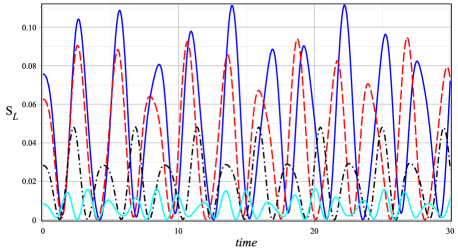
Figure 1: (color online) The effect of magnetic field on the dynamics of mixedness with $J_{i}=1.1,J_{f}=0.9,\omega_{i,1}=1,\omega_{f,1}=1.3,\omega_{i,2}=1.5$, $\omega_{f,2}=1.8$, $\omega_{c}=0$ (blue solid line), $\omega_{c}=0.3$ (red dashed line), $\omega_{c}=0.8$ (black dashed-dotted line), $\omega_{c}=1.5$ (cyan solid line).

The quenched value of the coupling parameter $J_{f}$ plays an interesting role in the dynamics of mixedness. In Figure 2 we show that when $\omega_{c}=0.2$, $J_{i}=1.1$ and $(\omega_{i,1}=1,\omega_{i,2}=1.5)\longrightarrow(\omega_{f,1}=1.3,\omega_{f,2}=1.8)$ the marginal states will be more mixed as the coupling parameter increases. For $J_{f}\leq 0.5$ the correlations between two subsystems are very weak and the mixedness presents a tiny sinusoidal oscillations behavior, which is due to the fact that a weak coupling $J\longrightarrow 0$ yields to $\phi\longrightarrow 0$ and eventually $S_{L}\longrightarrow 0$. Increasing $J_{f}$, the dynamics of $S_{L}$ periodic oscillations exhibit an increasing of amplitude and decreasing of frequency. For a large coupling these oscillations take an exponential dynamics, which is due to the nonphysical oscillations of the first oscillator (i.e. $\sigma_{1}\in\mathbb{C}$), then trigonometric functions $(\cos,\sin)$ in $h_{1}$ transform as $(\cosh,\sinh)$. But it is important to notice that this effect can be removed with a suitable choice of $\omega_{c}$ that allow us to construct exponential solutions of Ermakov equations [46] in order to follow the dynamics of time dependent harmonic oscillators.

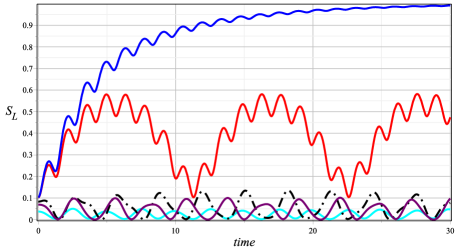
Figure 2: (color online) The effect of quenched coupling parameter $J_{f}$ on the dynamics of mixedness with $J_{i}=1.1,\omega_{i,1}=1$, $\omega_{f,1}=1.3$ $\omega_{i,2}=1.5$, $\omega_{f,2}=1.8$, $\omega_{c}=0.2$, $J_{f}=0.5$ (cyan solid line), $J_{f}=0.9$ (purple solid line), $J_{f}=1.2$ (black dotted-dashed line), $J_{f}=2.3$ (red solid line), $J_{f}=2.4$ (blue solid line).

In Figure 3 we present the effect of quenched coupling frequency $\omega_{f,2}$ on the dynamics of mixedness. We observe that the mixedness undergoes an amplitude frequency modulation, decreases as the quenched frequency increases and eventually the oscillations disappear while the dynamics becomes exponential. Finally, it appears that the magnetic field plays an important role in purification of marginal states and gives rise to the physical oscillations with high correlations. We observe that a large coupling yields quickly to maximally mixed states and the small values of the quenched frequencies lead to maximally marginal mixed states.

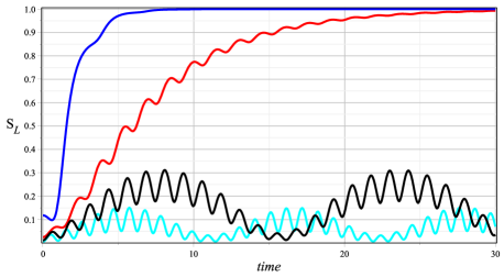
Figure 3: (color online) The effect of quenched coupling frequency $\omega_{f,2}$ on the dynamics of mixedness with $J_{i}=1.1,J_{f}=0.9,\omega_{i,1}=1,\omega_{i,2}=1.5$, $\omega_{f,1}=0.4$, $\omega_{c}=0.1$, $\omega_{f,2}=3$ (cyan solid line), $\omega_{f,2}=2.5$ (black solid line), $\omega_{f,2}=2$ (red solid line), $\omega_{f,2}=0.5$ (blue solid line).

7.2 Dynamics of phase space fluctuations

To graphically study the dynamics of uncertainty, we plot the variation of $U_{1}=\left(2\Delta x_{1}\Delta x_{2}\right)^{2}$ versus time under suitable conditions. Firstly, we investigate the effect of magnetic field on such dynamics in Figure 4 by taking a fix quench $(\omega_{i,1}=1,\omega_{i,2}=1.5,J_{i}=1.1)\longrightarrow(\omega_{f,1}=1.3,\omega_{f,2}=1.8,J_{f}=0.9)$ and different values of $\omega_{c}=0,0.3,0.8,1.5$. For $\omega_{c}=0$ the dynamics of uncertainty presents a multi-oscillatory behavior, which is due to solutions of the Ermakov equations and their derivatives. Increasing $\omega_{c}$ undergoes the dynamics to oscillate in the vicinity of minimality. We conclude from our analysis that uncertainty can be assisted via a static magnetic field and eventually handle the quantum fluctuations.

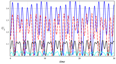
Figure 4: (color online) The effect of magnetic field on the dynamics of uncertainty $U_{1}=(2\Delta x_{1}\Delta p_{1})^{2}$ with $J_{i}=1.1,J_{f}=0.9,\omega_{i,1}=1,\omega_{f,1}=1.3,\omega_{i,2}=1.5$, $\omega_{f,2}=1.8$, $\omega_{c}=0$ (blue solid line), $\omega_{c}=0.3$ (red dashed line), $\omega_{c}=0.8$ (black solid line), $\omega_{c}=1.5$ (cyan solid line).

Secondly, we show the impact of the quenched coupling parameter $J_{f}$ on the dynamics of uncertainty $U_{1}=(2\Delta x_{1}\Delta p_{1})^{2}$ in Figure 5. It is clearly seen that for small values of the coupling, the dynamics of uncertainty exhibits a periodic behavior. However, for a large coupling such dynamics exhibits a bi-sinusoidal behavior with a large amplitude and small frequency. From the critical value $J_{f}=2.4$ the oscillations disappear and the behavior become exponential, which is quite natural because as we have seen previously for mixedness, $J_{f}=2.4$ yields to $S_{L}\longrightarrow 1$ and from Eq. (75) the first term goes to infinity, i.e. $\frac{1}{(1-S_{L})^{2}}\longrightarrow+\infty$. Note that, the lower bound of uncertainty $\frac{1}{2}(1+\gamma_{1}^{2}(t,\omega_{c}))^{\frac{1}{2}}$ strongly depends on the magnetic field and time, which is very important to preserve the invariance of uncertainty with respect to phase space transformations during the action of the magnetic field and dynamics. Such lower bound is the same as that obtained using the Robertson-Schrödinger uncertainty [7].

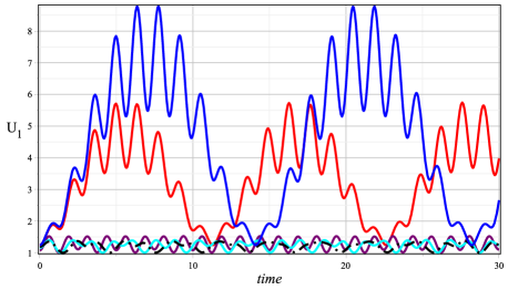
Figure 5: (color online) The effect of magnetic field on the dynamics of uncertainty $U_{1}=(2\Delta x_{1}\Delta p_{1})^{2}$ with $J_{i}=1.1,\omega_{i,1}=1,\omega_{f,1}=1.3,\omega_{i,2}=1.5$, $\omega_{f,2}=1.8$, $\omega_{c}=0.2$, $J_{f}=0.5$ (purple solid line), $J_{f}=0.9$ (cyan solid line), $J_{f}=1.2$ (black dotted-dashed line), $J_{f}=2.3$ (red solid line), $J_{f}=2.33$ (blue solid line).

Thirdly, we show the effects of quenched frequency $\omega_{f,2}$ on the dynamics of uncertainty $U_{1}=(2\Delta x_{1}\Delta p_{1})^{2}$ in Figure 6 for different quenches $(\omega_{i,1}=1,\omega_{i,2}=1.5,J_{i}=1.1)\longrightarrow(\omega_{f,1}=0.4,\omega_{f,2}=2.3,2.5,3,4,J_{f}=0.9)$. We observe that for $\omega_{f,2}=0.5,2$, the uncertainty presents a large uncertainty with exponential behavior, which is trivial because the dynamics drives $S_{L}$ to $1$ then $U_{1}\longrightarrow+\infty$. It is interesting to notice that a large $\omega_{f,2}$ yields to the pure marginals and the lower bound will be saturated. We conclude that the fluctuations depend on the magnetic field, coupling parameter and quenched frequencies. When the mixedness is minimal, the uncertainty is also because a tiny mixedness means that the lack of information is very small then the fluctuations are minimal.

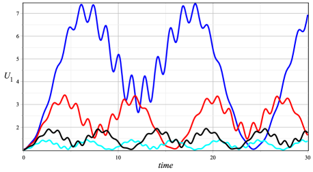
Figure 6: (color online) The effect of quenched coupling frequency $\omega_{f,2}$ on the dynamics of uncertainty $U_{1}=(2\Delta x_{1}\Delta p_{1})^{2}$ with $J_{i}=1.1,J_{f}=0.9,\omega_{i,1}=1,\omega_{i,2}=1.5$, $\omega_{f,1}=0.4$, $\omega_{c}=0.1$, $\omega_{f,2}=4$ (cyan solid line), $\omega_{f,2}=3$ (black solid line), $\omega_{f,2}=2.5$ (red solid line), $\omega_{f,2}=2.3$ (blue solid line).

7.3 Dynamics of entanglement via $S_{von}$ and $\mathcal{N}$

Our global state is pure and Gaussian, thus to study the dynamics of entanglement we use two quantifiers. First one is the von Neumann Entropy or generally the Rényi Entropies $S_{R}^{\nu}(\rho^{A}_{(0,0)})=\frac{1}{1-\nu}\ln{\rm Tr}\left[\left(\rho_{(0,0)}^{A}\right)^{\nu}\right]$, where $S_{von}=\lim_{\nu\rightarrow 1}S_{R}^{\nu}$ [4, 11], and second is the logarithmic negativity $\mathcal{N}$ [1, 11]. The later quantifier presents a lot of simplifications because its measure does not involve the resolution of spectral equations Eq. (37) and addresses only to the marginal purities and some symplectic parameters of CM. Moreover, in our case TDGE is symmetric then $\mathcal{N}$ will be expressed only in term of marginal purity ${\rm Tr}\left[\left(\rho_{(0,0)}^{A}\right)^{2}\right]$. To graphically show the dynamics of the amount of entanglement encoded in the reduced states $\left(\rho^{A}_{(0,0)},\rho^{B}_{(0,0)}\right)$ we plot both quantities $S_{von}$ and $\mathcal{N}$ versus time.

Firstly, we investigate the effect produced by a magnetic field in Figure 7 by taking fix quenches $(\omega_{i,1}=1,\omega_{i,2}=1.5,J_{i}=1.1)\longrightarrow(\omega_{f,1}=1.3,\omega_{f,2}=1.8,J_{f}=0.9)$ and different values of $\omega_{c}=0,0.3,0.8,1.5,3$. For $\omega_{c}=0$, $S_{von}$ and $\mathcal{N}$ exhibit a similar topological behavior (the same variations). For $\omega_{c}=0.3,0.8,1.5,1.3$, the magnetic field creates an important decreasing on the amplitude of $S_{von}$ and $\mathcal{N}$. Thus the entanglement can be remoted by the magnetic field and $\omega_{c}$ affects violently the frequency of both oscillations, which is natural because of the phase $\sim\omega_{c}t$ presented in solutions of the Ermakov equations. This tell us the magnetic field can be used to control the information delivered by $S_{von}$ and $\mathcal{N}$.

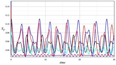
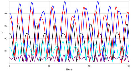
Figure 7: (color online) The effect of magnetic field on the dynamics of von Neumann entropy $S_{von}$ and logarithmic negativity $\mathcal{N}$ with $J_{i}=1.1,\,J_{f}=0.9,\omega_{i,1}=1,\omega_{f,1}=1.3,\,\omega_{i,2}=1.5$, $\omega_{f,2}=1.8$, $\omega_{c}=0$ (blue solid line), $\omega_{c}=0.3$ (red solid line), $\omega_{c}=0.8$ (black solid line), $\omega_{c}=1.5$ (cyan solid line), $\omega_{c}=3$ (purple solid line).

Secondly, we explore the impact of the quenched coupling $J_{f}$ on the dynamics of entanglement in Figure 8. Note that, if $J=0$ then $\phi=0$ and $S_{von}=\mathcal{N}=0$ showing that the coupling $J_{f}$ witnesses the existence of entanglement. Now increasing $J_{f}$ to $0.5$ and $0.9$, the entanglement dynamics undergoes an amplitude frequency modulation: the amount of entanglement becomes more important and exhibits a bi-sinusoidal behavior, which due to solutions of the Ermakov equations. We observe that a large coupling $J_{f}$ yields to the nonphysical oscillations (negativity of the square of frequency) $\sigma_{1}\in\mathbb{C}$, which leads to $S_{L}\rightarrow+\infty$ then $\mathcal{N},S_{von}\longrightarrow+\infty$.

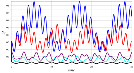
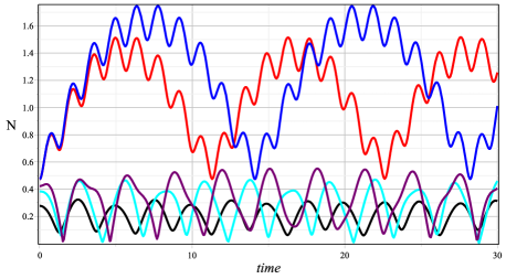
Figure 8: (color online) The effect of quenched coupling $J_{f}$ on the dynamics of von Neumann $S_{von}$ entropy and logarithmic negativity $\mathcal{N}$ with $J_{i}=1.1,\omega_{i,1}=1,\,\omega_{f,1}=1.3,\omega_{i,2}=1.5$, $\omega_{f,2}=1.8$, $\omega_{c}=0.2$, $J_{f}=0.5$ (black solid line), $J_{f}=0.9$ (cyan solid line), $J_{f}=1.2$ (purple solid line), $J_{f}=2.3$ (red solid line), $J_{f}=2.33$ (blue solid line).

Thirdly, we show the variations of $S_{von}$ and $\mathcal{N}$ versus time with respect to quenched frequency $\omega_{f,2}$ (without loss of generality) in Figure 9. The dynamics shows that if we increase $\omega_{f,2}$ the amount of entanglement decreases because if $\omega_{f,2}$ increases then the difference $|\omega_{f,1}^{2}-\omega_{f,2}^{2}|$ becomes large implying that the separability is reached. Moreover, two entangled microscillators should have the same mechanical features. It is interesting to notice that the three dynamics are linked and present the same topological behavior with respect to $\omega_{c},J_{f}$, $\omega_{f,2}$ and similar dynamics.

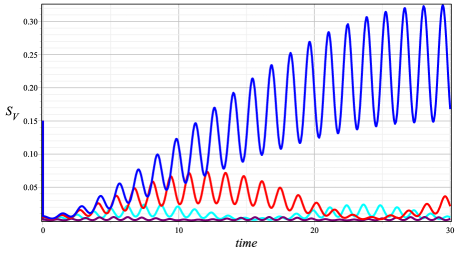
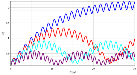
Figure 9: (color online) The effect of quenched frequency $\omega_{f,2}$ on the dynamics of von Neumann $S_{von}$ entropy and logarithmic negativity $\mathcal{N}$ with $J_{i}=1.1,\omega_{i,1}=1,\omega_{f,1}=1.3,\omega_{i,2}=1.5$, $\omega_{f,2}=1.8$, $\omega_{c}=0.1$, $\omega_{f,2}=3$ (purple solid line), $\omega_{f,2}=2.5$ (cyan solid line), $\omega_{f,2}=2.3$ (red solid line), $\omega_{f,2}=2.2$ (blue solid line).

8 Conclusion

We have considered time dependent harmonic oscillator subject to a static magnetic field and studied the dynamics of entanglement, mixedness and logarithmic negativity. Firstly, we have used the rotation $SO(2)$ in the phase plane $(x,p)$ to diagonalize the Hamiltonian. We have derived the solutions $\Psi_{n,m}$ of TDSE of our system and focused only on the vacuum state $\Psi_{0,0}$ by showing that it is TDGS, symmetric and pure state. This was used to show that the von Neumann entropy $S_{von}$ and logarithmic negativity $\mathcal{N}$ are legitimate quantifiers of entanglement. Furthermore, we have computed the common marginal purity and further the linear entropy $S_{L}$ to quantify the degree of mixedness. In addition, we have employed the Heisenberg uncertainty to study the dynamics of uncertainties and eventually demonstrated explicit relations between the entanglement, mixedness and uncertainty, which allowed us to use the purity or mixedness as suitable candidates of the required quantifiers.

Subsequently, we have studied the dynamics of the entanglement, mixedness and uncertainty using the quenched model [3, 4] in order to derive the solutions $h_{i}$ of the Ermakov equations and their time derivatives $\dot{h}_{i}$, $i=1,2$. We have shown that the magnetic field purifies the marginal states thus decreasing the amount of quantum correlations, a feature that can be used to control and handle these prototypical states. We have demonstrated also that the three quantities (entanglement, mixedness, logarithmic negativity) present the same behavior with respect to the magnetic field, which leads to construct a meaningful quantifier mixedness-based. We have shown also that the uncertainty approaches to saturate that is lower bound in the vicinity of separable states $\mathcal{N},S_{von}\rightarrow 0$, an issue used to detect experimentally the entangled states.

References

• [1] L. Amico, R. Fazio, A. Osterloh and V. Vedral, Rev. Mod. Phy. 80, 517 (2008).
• [2] A. Peres, Quantum Theory: Concepts and Methods (Kluwer, Dordrecht, 1993).
• [3] S. Ghosh, Europhys. Lett. 120, 50005 (2017).
• [4] D. Park, Quantum Inf. Process. 17 (6), 147 (2018).
• [5] A. Jellal and A. Merdaci, Entropies for Coupled Harmonic Oscillators and Temperature 2019, arXiv:1902.07645.
• [6] N. Friis, G.Vitagliano, M. Malik and M. Huber, Nat. Rev. Phys. 1, 72 (2019).
• [7] A. Hertz and N. J. Cerf, J. Phys. A: Math. Theor. 52, 173001 (2019).
• [8] W. Heisenbeg, Z. Phy. 43, 172 (1927).
• [9] H. P. Robertson, Phy. Rev. A 667, 35 (1930).
• [10] I. B. Birula, AIP Conference Proceedings 889, 52 (2007).
• [11] G. Adesso, A. Serafini and F. Illuminati, Phys. Rev. A 70, 022318 (2004).
• [12] D. Sen, Current Science 107, 2 (2014).
• [13] H. R. Lewis Jr, Phys. Rev. Lett. 18, 510 (1967).
• [14] H. R. Lewis Jr and B. Riesenfeld, J. Math. Phys. 10, 1458 (1969).
• [15] A. Lohe, J. Phys. A: Math. Theor. 42, 035307 (2009).
• [16] J. R. Burgan, M. R. Feix, E. Fijalkow and A. Munier, Phys. Lett. A 74, 11 (1979).
• [17] D. N. Makarov, Scientific Reports 8, 8204 (2018).
• [18] O. M. Del Cima, D. H. T. Franco and M. M. Silva, Quantum Stud.: Math. Found. 6, 141 (2019).
• [19] D. Han, Y. S. Kim and M. E. Noz, Coupled Harmonic Oscillators and Feynman’s Rest of the Universe (1997), cond-mat/9705029.
• [20] D. Han, Y. S. Kim and M. E. Noz, Phys. Rev. A 41, 6233 (1990).
• [21] A. A. Bykov, G. M. Gusev, J. R. Leite, A. K. Bakarov, A. V. Goran, V. M. Kudryashev and A. I. Toropov, Phys. Rev. B 65, 035302 (2001).
• [22] T.A. Kennedy, R. Wagner, B. McCombe and D. Tsui, Phys. Rev. Lett. 35, 1031 (1975).
• [23] R. K. Colegrave and M. A. Mannan, J. Math. Phys. 29, 1580 (1988).
• [24] H. Moya-Cessa, F. Soto-Eguibar, J. M. Vargas-Martinez, R. Juarez-Amaro and A. ZuΓ±iga-Segundo, Phys. Rep. 513, 229 (2012).
• [25] C. K. Law, Phys. Rev. A 49, 433 (1994).
• [26] X. Chen, A. Ruschhaupt, S. Schmidt, A. del Campo, D. GuΓ©ry-Odelin and J. G. Muga, Phys. Rev. Lett. 104, 063002 (2010).
• [27] C. W. Duncan and A. del Campo, New J. Phys. 20, 085003 (2018).
• [28] V. V. Dodonov and A. B. Klimov, Phys. Rev. A 54, 2664 (1996).
• [29] R. RomΓ‘n-Ancheyta, I. Ramos-Prieto, A. Perez-Leija, K. Busch and R. D. J. LeΓ³n-Montiel, Phys. Rev. bf A 96 , 032501 (2017).
• [30] C. Kiefer, J. Marto and P. V. Moniz, Ann. Phys. 18, 722 (2012).
• [31] D. N. Makarov, Phys. Rev. E 97, 042203 (2018).
• [32] S. Menouar, M. Maamache and J. R. Choi, Ann. Phys. 325, 1708 (2010).
• [33] H. Goldstein, Classical Mechanics (Addison-Wesley, Reading, MA, 1980).
• [34] M. Boudjema-Bouloudenine, T. Boudjedaa and A. Makhlouf, Eur. Phys. J. C 46, 807 (2006).
• [35] D. Han, Y. S. Kim and Marilyn E. Noz, Am. J. Phys. 67, 61 (1999).
• [36] A. Jellal, E. H. El Kinani and M. Schreiber, Int. J. Mod. Phys. A 20, 1515 (2005).
• [37] A. Jellal, F. Madouri and A. Merdaci, J. Stat. Mech. P09015 (2011).
• [38] A. Merdaci, A. Jellal, A. Al Sawalha and A. Bahaoui, J. Stat. Mech. P093101 (2018).
• [39] A. Merdaci and A. Jellal, Phys. Lett. A 384, 126134 (2020).
• [40] M. Srednicki, Phys. Rev. Lett. 71, 666 (1993).
• [41] L. Bombelli, R. K. Koul, J. Lee and R. D. Sorkin Phys. Rev. D 34, 374 (1986).
• [42] G. Vidal and R. F. Werner, Phy. Rev. A 65, 032314 (2002).
• [43] K. Zyczkowski, P. Horodecki, A. Sanpera and M. Lewenstein, Phy. Rev. A 58, 883 (1998).
• [44] Lu-Ming Duan, G. Giedke, J. I. Cirac and P. Zoller, Phys. Rev. Lett. 84, 2722 (2000).
• [45] M. J. Bastiaans, J. Opt. Soc. Am 1, 711 (1984).
• [46] S. P. Kim and W. Kim, J. Korean Phys. Soc. 69, 1513 (2016).