DDTF for CS-MRI via Off-the-Grid RegularizationJian-Feng Cai, Jae Kyu Choi, and Ke Wei
Data Driven Tight Frame for Compressed Sensing MRI Reconstruction via Off-the-Grid Regularization††thanks: Submitted to the editors DATE. \fundingThe research of the first author is supported by the Hong Kong Research Grant Council Grant 16306317. The research of the second author is supported in part by the NSFC Youth Program 11901436. The research of the third author is supported by the NSFC Youth Program 11801088.
Abstract
Recently, the finite-rate-of-innovation (FRI) based continuous domain regularization is emerging as an alternative to the conventional on-the-grid sparse regularization for the compressed sensing (CS) due to its ability to alleviate the basis mismatch between the true support of the shape in the continuous domain and the discrete grid. In this paper, we propose a new off-the-grid regularization for the CS-MRI reconstruction. Following the recent works on two dimensional FRI, we assume that the discontinuities/edges of the image are localized in the zero level set of a band-limited periodic function. This assumption induces the linear dependencies among the Fourier samples of the gradient of the image, which leads to a low rank two-fold Hankel matrix. We further observe that the singular value decomposition of a low rank Hankel matrix corresponds to an adaptive tight frame system which can represent the image with sparse canonical coefficients. Based on this observation, we propose a data driven tight frame based off-the-grid regularization model for the CS-MRI reconstruction. To solve the nonconvex and nonsmooth model, a proximal alternating minimization algorithm with a guaranteed global convergence is adopted. Finally, the numerical experiments show that our proposed data driven tight frame based approach outperforms the existing approaches.
keywords:
Magnetic resonance imaging, finite-rate-of-innovation, structured low rank matrix completion, (tight) wavelet frames, data driven tight frames, proximal alternating schemes42B05, 65K15, 65R32, 68U10, 90C90, 92C55, 94A12, 94A20
1 Introduction
Magnetic resonance imaging (MRI) is one of the most widely used medical imaging modality in clinical diagnosis [34]. It is non-radioactive, non-invasive, and has excellent soft tissue contrasts such as T1 and T2 with high spatial resolution [43]. Among these merits, the availability of high spatial resolution images, which will be the focus of this paper, facilitates early diagnosis by enabling the detection and characterization of clinically important lesions [50, 61]. However, since the so-called k-space data acquisition is limited due to physical (gradient amplitude and slew-rate) and physiological (motion artifacts due to the patient’s respiratory motion which can generate the outlier of the k-space data) constraints [37, 40, 43, 46], there has been increasing demand for methods which can reduce the amount of acquired data without degrading the image quality [46].
When the k-space data is undersampled, the Nyquist sampling criterion is violated, and the direct restoration using this undersampled k-space data will lead to the aliasing in the reconstructed image [46]. In the literature, the famous compressed sensing (CS) MRI can be viewed as a sub-Nyquist sampling method which exploits the sparse representation of an image to compensate the undersampled k-space data [21, 28, 37, 46]. More precisely, a typical norm based “on-the-grid” CS-MRI model restores the MR image on the grid, by regularizing smooth image components while preserving image singularities such as edges, ridges, and corners.
Even though the conventional on-the-grid approaches have shown strong ability to reduce the data acquisition time and thus received a lot of attention over the past few years [43], they have to be further improved as the k-space data is a discrete (and truncated) sampling of a Fourier transform of an underlying function in the continuous domain, under the assumption of a single-coil MRI [34]. This means that, the sparse regularization based image restoration will work well when the singularities of the image are well aligned with the grid. However, even in the case of piecewise constant function whose (distributional) gradient is sparse in the continuous domain, its singularities may not necessarily agree with the discrete grid, leading to the problem of basis mismatch [24, 51, 70]. Such a basis mismatch between the true singularities and the discrete grid may result in the loss of sparse structure of the image, and thus degrades the restoration quality [70].
1.1 Continuous domain regularization for image restoration
The continuous domain regularization is emerging as a powerful alternative to the discrete domain sparse regularization [7, 19, 23, 48]. By such an “off-the-grid” scheme, the regularization on the discrete data exploits the sparsity in the continuous domain to alleviate the basis mismatch, which is especially attractive in signal restorations from partial measurements [48]. One of the most successful examples is the finite-rate-of-innovation (FRI) framework which corresponds a superposition of a few sinusoids to a low rank Hankel matrix [8]. Similarly, we can adopt the so-called structured low rank matrix completion (SLMC) [23, 52, 69] for the CS restoration based on the continuous domain regularization. The SLMC approach can also be used to restore Fourier samples of a one dimensional piecewise constant signal [8, 64] by considering the Fourier samples of a derivative. However, while this framework works well in the case of isolated singularities [18, 67], the extension to the (piecewise smooth) image restoration is not straightforward [51]. This is because the image singularities such as the edges and ridges in general form a continuous curve in a two dimensional domain, which makes it challenging to construct a structured low rank matrix from the Fourier samples.
Recently, there are several extensions of the FRI framework to two dimensional continuous domain regularization for image restoration. Such extensions include the piecewise holomorphic complex image restoration [53] and the piecewise constant real image restoration [48, 49, 50, 51]. These approaches are commonly based on the assumption that the singularity curves, i.e. the supports of the (real/complex) derivatives of a target image, lie in the zero level set of a band-limited periodic function, called the annihilating polynomial. Indeed, given that the edges lie in the zero level set of an annihilating polynomial, the structured matrix (Hankel/Toeplitz matrix) constructed from the Fourier samples of piecewise constant images becomes low rank [48, 50, 51]. Hence, in CS-MRI, we can first restore the fully sampled k-space data (the discrete sample of the Fourier transform of a piecewise constant function) via the SLMC, and then restore MR image by the inverse DFT [35, 39].
Though the rank minimization problem is an NP-hard problem in general [20], numerous tractable relaxation approaches have been proposed for the SLMC. One of them is the convex nuclear norm relaxation method (e.g. [15, 29]), together with the theoretical restoration guarantees (e.g. [48]). In addition, the iterative reweighted least squares (IRLS) approaches for the Schatten -norm minimization are proposed in [31, 47, 52], which can avoid the high computational cost of the SVD related to the rank minmization and the convex nuclear norm relaxation. Apart from these approaches, the nonconvex alternating projection methods based on the different parametrizations of the underlying low rank matrix structure are proposed and studied in [16, 17]. These nonconvex methods are reported to be superior to the other relaxation methods in terms of the computational efficiency while theoretical restoration guarantees are still available.
1.2 Motivations and contributions of our approach
Our proposed off-the-grid approach for the CS-MRI restoration is based on the fact that the SVD of a Hankel matrix induces tight frame filter banks due to its underlying convolutional structure. This means that, if we can associate a signal with a low rank Hankel matrix, its right singular vectors form tight frame filter banks which allow us to represent the signal with sparse canonical coefficients. Hence, instead of directly minimizing the rank of a two-fold Hankel matrix, we can develop the sparse regularization model via data driven tight frames [13] for the CS-MRI restoration. More specifically, using the norm of the frame coefficients, we propose the balanced approach [11, 22] as a relaxation of the low rank two-fold Hankel matrix approximation which is based on the framework of annihilating filters. Finally, the numerical experiments show that our data driven tight frame approach outperforms the structured low rank matrix approaches (and their relaxations) as well as the existing on-the-grid approaches, leading to the state-of-the-art performance.
Note that the data driven tight frame as well as the dictionary learning has been discussed for the various image restoration tasks. More precisely, the data driven tight frame is first used for the image denoising [13], the multi-channel image denoising and inpainting [65], the joint spatial-Radon domain regularization for the sparse view CT [71], and the PET-MRI joint reconstruction [25]. In addition, the authors in [60] explored the general framework of the dictionary learning based image restoration model with the convergence analysis. However, while these aforementioned approaches mainly concern the sparse approximation of the discrete images, to the best of our knowledge, our approach for the first time applies the data driven tight frame regularization to the MRI restoration based on a continuous image model.
Finally, we would like to mention that the proposed off-the-grid approach for the CS-MRI restoration is not limited to the two dimensional single-coil MRI restoration. Even though further numerical studies are required, it is not hard to generalize the proposed model to the three dimensional cases. In addition, since the multiplication in the image domain becomes the convolution in the frequency domain via the Fourier transform, we can extend our approach to a SENSE setup [57], a multiple-coil MRI restoration whose inverse problem corresponds to the multi-channel deconvolution in the frequency domain with a known coil sensitivity map.
1.3 Organization and notation of paper
The rest of this paper is organized as follows. We first briefly review the tight wavelet frames including the wavelet frame based image restorations and the data driven tight frames in Section 2. Section 3 begins with the review on the structured low rank matrix approaches for CS-MRI. Then we present the off-the-grid CS-MRI reconstruction approach based on data driven tight frames, followed by the alternating minimization algorithm. In Section 4, experimental results are reported to demonstrate the performance of our new CS-MRI restoration method, and Section 5 concludes this paper with a few future directions.
Throughout this paper, all two dimensional discrete images will be denoted by the bold faced lower case letters while the functions in a two dimensional continuous domain will be denoted by regular characters. Note that a two dimensional image can also be identified with a vector whenever convenient. All matrices will be denoted by the bold faced upper case letters, and the th row and the th column of a matrix will be denoted by and , respectively. We denote by
| (1.1) |
with , the set of grid, and the space of complex valued functions on is denoted by . Given two rectangular grids and , the contraction is defined as
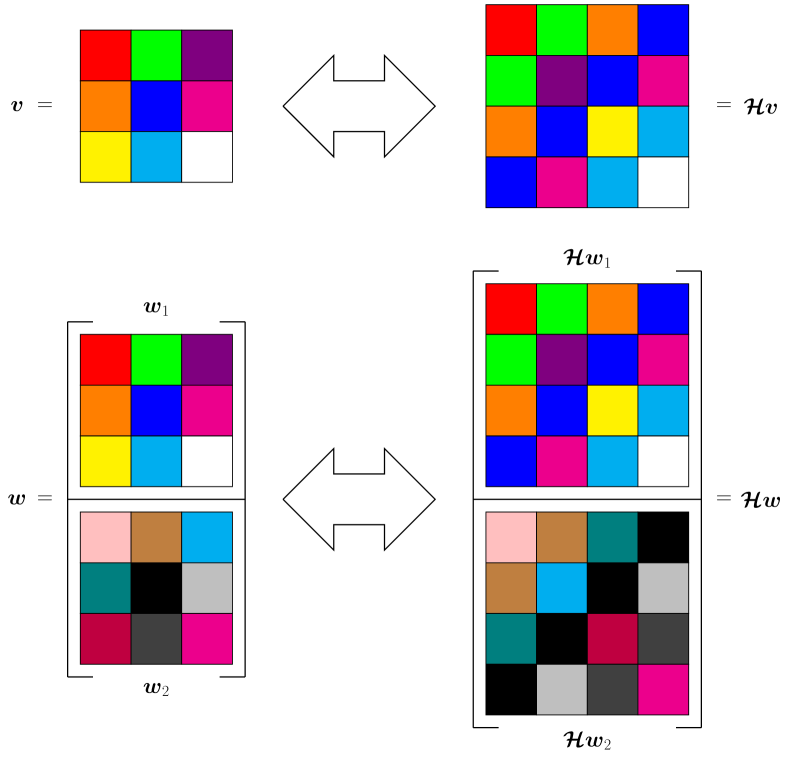
Finally, operators are denoted as the bold faced calligraphic letters. For instance, let and let be a rectangular grid. The corresponding Hankel matrix is an matrix ( and ) generated by concatenating patches of into row vectors. In the sense of two dimensional multi-indices, we can formally write as
With a slight abuse of notation, we also use
| (1.3) |
to denote the two-fold Hankel matrix constructed from ; see Fig. 1 for an illustration.
2 Preliminaries on tight wavelet frames
Here we provide a brief introduction on tight wavelet frames and data driven tight frames. Interested readers may consult [11, 26, 27, 62, 63] for detailed surveys on tight wavelet frames, and [5, 13] for details on data driven tight frames. For the sake of simplicity, we only discuss the real valued wavelet tight frame systems, but note that it is not difficult to extend the idea to the complex case.
Denote by a Hilbert space and let be the inner product defined on . A countable set is called a tight frame on if
| (2.1) |
Given , we define the analysis operator as
The synthesis operator is defined as the adjoint of :
Then is a tight frame on if and only if where is the identity on . It follows that, for a given tight frame , we have the following canonical expression:
with being called the canonical tight frame coefficients. Hence, the tight frames are extensions of orthonormal bases to the redundant systems. In fact, a tight frame is an orthonormal basis if and only if for all .
One of the most widely used class of tight frames is the discrete wavelet frame generated by a set of finitely supported filters . Throughout this paper, we only discuss the two dimensional undecimated wavelet frames on , but note that it is not difficult to extend to with . For , define a convolution operator by
| (2.2) |
Given a set of finitely supported filters , define the analysis operator and the synthesis operator by
| (2.3) | ||||
| (2.4) |
respectively. Then, the direct computation can show that the rows of form a tight frame on (i.e. ) if and only if the filters satisfy
| (2.7) |
called the unitary extension principle (UEP) condition [36]. Finally, for a two dimensional discrete image on the finite grid, in Eq. 2.2 with a finitely supported denotes the discrete convolution under the periodic boundary condition throughout this paper.
In the literature, wavelet frames are widely used for the sparse approximation of an image. To explore a better sparse approximation, the authors in [13] proposed a data driven tight frame approach, inspired by [1, 59]. Specifically, given a two dimensional image , a tight frame system defined as in Eq. 2.3, which is generated by a set of finitely supported filters supported on a grid and satisfying Eq. 2.7, is constructed via the following minimization
| (2.8) |
with the norm encoding the number of nonzero entries in the coefficient vector . Note that in wavelet domain, there is usually a set of low pass coefficients that are not sparse. In fact, through the relaxation of Eq. 2.8 which will be discussed below, we can learn a tight frame system by fixing a low pass filter and penalizing the norm of high pass coefficients only, following [3]. However, since the main focus is to establish a relation between the tight frame filter banks and the Hankel matrix, we forgo further discussions on such a detailed construction.
To solve Eq. 2.8, the authors in [13] presented that if satisfies , after reformulating into filters supported on , its column vectors generate filters satisfying the UEP condition Eq. 2.7. Hence, under such an assumption on the filters , we can rewrite Eq. 2.8 as
| (2.9) |
to construct filter banks. Here, is a Hankel matrix generated by the patches of , is the corresponding matrix formulation of , and is the Frobenius norm of a matrix. To solve Eq. 2.9, the alternating minimization method with closed form solutions for each stage is presented in [13]. In addition, the proximal alternating minimization (PAM) scheme with global convergence to critical points is proposed in [5].
3 Proposed off-the-grid regularization model
3.1 Structured low rank matrix approaches in CS-MRI
We begin with the brief review on the structured low rank matrix approaches in CS-MRI. Interested readers can refer to [51] and references therein for more detailed surveys. Throughout this paper, we only consider the two dimensional single-coil MRI reconstruction for the sake of simplicity, so that the k-space data can be modeled as
| (3.1) |
where is the sampling region, is the length of field-of-view (FOV), and is the proton spin density distribution in [34]. We further assume that is supported on . This means that when in Eq. 3.1 is available for , we have
In general, the k-space data can be sampled at “arbitrary” positions, i.e. . However, to simplify the discussion, we assume that where is defined as Eq. 1.1, i.e. the discrete sampling on the Nyquist rate grid [34, 41].
The conventional CS-MRI approach aims to directly restore the MR image on from the k-space undersampled on . Note that when , i.e. the fully sampled case, is obtained from the inverse DFT
| (3.2) |
Hence, the conventional sparse regularization based CS-MRI approach
| (3.3) |
is based on the DFT
| (3.4) |
Here, is a restriction onto , and is a sparsifying transformation. Note that Eq. 3.3 is the on-the-grid scheme, as we promote the sparsity of the discrete image on the grid . In other words, we can apply the sparse regularization effectively provided that the singularities of are well aligned with . However, since the k-space data actually comes from the Fourier transform of a continuous domain function , together with Eq. 3.1 and , Eq. 3.2 can be rewritten as
where is the Dirichlet kernel defined as
In other words, since the MR image is proportional to a discrete sampling of on rather than that of [34], there exists a basis mismatch between the singularities of in the continuous domain and the discrete grid . Such a basis mismatch would destroy the sparsity structure, leading to a degradation of the restoration performance.
Instead of directly restoring the discrete MR image, the off-the-grid approaches attempt to first restore the fully sampled k-space data from its undersampled version modeled as in Eq. 3.1. Formally, we can write the problem as follows:
| (3.5) |
and then compute by using the restored k-space data .
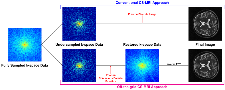
Generally, it is impossible to directly solve Eq. 3.5 without any further information. Nevertheless, by imposing the prior information of (in the continuous domain) into Eq. 3.5, we can exploit the continuous domain regularization, and reduce the basis mismatch; see Fig. 2 for the schematic comparison. For this purpose, we follow [51] and consider the following piecewise constant function model of the proton density :
| (3.6) |
where and denotes the characteristic function on a set : if , and otherwise. We further assume that each lies in , and Eq. 3.6 is expressed with the smallest number of characteristic functions such that ’s are pairwise disjoint. Then the discontinuities of agrees with , called the edge set of [51]. Under this setting, the authors in [50, 51] derived the following linear annihilation relation.
Proposition 3.1.
Let be a piecewise constant function defined as Eq. 3.6. Assume that there exists a finite (rectangular and symmetric) index set such that
| (3.7) |
Then for such , the Fourier transform of is annihilated by the convolution with the Fourier transform of . More precisely, we have
| (3.8) |
where the convolution acts on and separately.
The trigonometric polynomial in Eq. 3.7 is called the annihilating polynomial, is called the annihilating filter with support , and satisfying Eq. 3.7 is called the trigonometric curves [51]. It is proved in [51] that trigonometric curves can always be described as the zero set of a real valued trigonometric polynomial, using the tool of algebraic geometries.
In MRI, the Fourier transform of is sampled on the grid , so Eq. 3.8 becomes the finite system of linear equations
| (3.9) |
In the matrix-vector multiplication form, we have
| (3.10) |
Moreover, if in Eq. 3.7 is the minimal polynomial with the support (i.e. has the smallest linear dimension) and is the assumed filter support strictly containing , then we have
| (3.11) |
Roughly speaking, Eq. 3.11 means that if in Eq. 3.7 is the minimal polynomial with satisfying Eqs. 3.9 and 3.10, so does the translation for all , or equivalently, is also an annihilating polynomial. See [50, 51] for details.
Note that Eq. 3.11 means the two-fold Hankel matrix constructed by is rank deficient whenever the grid in Eq. 1.1 is large enough to satisfy the conditions in [51, Proposition 5.1]. Based on this observation, we can formulate Eq. 3.5 as the following low rank two-fold Hankel matrix completion [23, 52, 69]
| (3.12) |
Here, and is a weight matrix defined as
| (3.15) |
which is derived from the sample of on . Hence, the piecewise constant property of in the continuous domain can be transformed to the low rank property of .
3.2 Proposed CS-MRI model
Denote by the k-space data on the grid , which is to be restored from a given data undersampled on . Consider a two-fold Hankel matrix defined as Eq. 1.3 with defined as Eq. 3.15. To reconstruct corresponding to a piecewise constant function in Eq. 3.6, we assume that , following Section 3.1. Considering its SVD, we present Theorem 3.2, which is the key idea of the proposed CS-MRI model. The proof can be found in Appendix A.
To do this, we let be filters supported on , and we introduce
| (3.16) | ||||
| (3.17) |
where is a discrete convolution under the periodic boundary condition defined as Eq. 2.2. In other words, both and are concatenations of discrete convolutions.
Theorem 3.2.
Let be defined as in Eq. 3.6 and . Let be a two-fold Hankel matrix with defined as Eq. 3.15. Assume that . Considering its full SVD , we let by reformulating into a filter supported on . Then in Eq. 3.16 defined by using these satisfies
| (3.18) |
and for we have
| (3.19) |
where the discrete convolution acts on and separately111In fact, Eq. 3.19 is independent from the boundary condition of the discrete convolution, as is the grid where the boundary condition is inactive.. Consequently, if is of low rank, then its right singular vectors construct a tight frame under which is sparsely represented.
In words, Theorem 3.2 implies that a tight frame under which the weighted k-space data is sparse can be explicitly constructed from the SVD of the corresponding Hankel matrix, and the sparsity of the tight frame coefficients is grouped according to filters. Even though the Hankel matrix is not fully known in the CS-MRI setting since the k-space data is undersampled, Theorem 3.2 does motivate us to learn a better tight frame from the undersampled and noisy k-space data such that can be sparsely represented better. More precisely, we remove the group sparsity pattern in the canonical coefficients , and find the coefficients which are as sparse as possible. This leads to solving
| (3.20) | ||||
Here, is a tight frame transform defined as in Eq. 3.16, i.e. the concatenation of the convolutions with filter banks which have to be learned, and is a constraint set imposing the boundedness of . By relaxing the sparsity of tight frame coefficients over the entire range of (not necessarily in groups as in Eq. 3.19), we expect to achieve more flexibility, thereby leading to the improvements in restoration performance.
However, the direct penalization on the canonical coefficients requires an iterative solver, which will be too expensive in constructing an adaptive tight frame [13]. Therefore, by introducing an auxiliary variable , we approximate Eq. 3.20 by
| (3.21) | ||||
to learn the tight frame system and reconstruct the fully sampled k-space data on the grid simultaneously.
Remark 3.3.
For the constraint set , we choose
| (3.22) |
with a sufficiently large , and such a choice comes from the following: if is modeled as in Eq. 3.6, then the (distributional) gradient satisfies
where denotes the outward normal vector on , and denotes the surface measure. Since is a Radon vector measure on supported on , its Fourier transform is written as the Fourier transform of a measure (e.g. [30]):
which leads to
Hence, decays at infinity in the sense that
and this implies that (and whence since we want ) has to be bounded. In addition, as mentioned in e.g. [4], the boundedness constraint is required for the convergence guarantee of the proximal alternating scheme to solve Eq. 3.21. That being said, numerically, the constraint set has a very minor effect on the restoration results provided that is sufficiently large. In fact, the proximal alternating minimization seems to converge even without using .
Since our data driven tight frame approach is inspired by the SVD of a low rank , we expect the learned filters are related to the annihilating filters. More precisely, we expect , so that form an orthonormal basis for the null space of . Hence, following the arguments in [51], we can expect that the edge sets can also be restored from the learned filter banks as well. To see this, we let be the trigonometric polynomial defined as
where the filters are flipped because we use the two-fold Hankel matrix formulation. Given that the conditions in [51, Theorem 3.4] are satisfied, we can write where is the minimal polynomial in Eq. 3.7 and is another -periodic trigonometric polynomial. Following the similar arguments to [51, Proposition 5.3], for , we have
| (3.23) |
where
Hence, Eq. 3.23 shows that the learned filter banks are indeed related to the annihilating polynomials in the image domain.
Finally, we would like to mention that the application of dictionary learning to the CS-MRI reconstruction is already explored in [60]. Specifically, the authors in [60] proposed the following (unitary) sparsifying transform learning based CS-MRI (TLMRI) reconstruction model
| (3.24) | ||||
where represents an operator that extracts an patch of as a vector, denotes the number of patches, and denotes a square sparsifying transform for the patches of . Indeed, it seems that our proposed model Eq. 3.21 can also be classified into the dictionary learning based approach due to the data driven tight frame regularization. However, unlike the above TLMRI model Eq. 3.24 which considers the sparse structure of (the patches of) the underlying discrete image, the sparse regularization via data driven tight frame in Eq. 3.21 is a relaxation of the low rank two-fold Hankel matrix completion in the frequency domain, reflecting the piecewise constant function in a continuous domain via annihilating filters. Hence, Eq. 3.24 is an on-the-grid approach, whereas Eq. 3.21 is an off-the-grid approach.
3.3 Alternating minimization algorithm
To solve Eq. 3.21, we use the proximal alternating minimization (PAM) algorithm introduced in [2]. We initialize where
| (3.25) |
For , we can use the SVD of . However, to reduce the computational burden, we use the following way. Noting that we in general densely undersample the k-space data on the low frequencies based on the calibrationless sampling strategy, we restrict onto the smaller grid, for instance, . Then we compute the SVD , and set via
| (3.26) |
Using the initial filter banks as in Eq. 3.26, we initialize via
| (3.28) |
where is an estimated rank. After the initializations, we optimize alternatively, as summarized in Algorithm 1.
| (3.29) |
| (3.30) |
| (3.31) |
It is easy to see that each subproblem in Algorithm 1 has a closed form solution. Since for all , the solution to Eq. 3.29 is given by
| (3.32) | ||||
where is the adjoint of (i.e. the zero-filling operator), and is defined as Eq. 3.25. It is worth noting that since is a diagonal matrix, no matrix inversion is needed.
For the remaining subproblems Eqs. 3.30 and 3.31, we note that while the coefficients in Eq. 2.8 are intermediate variables to construct tight frame filter banks, the coefficients in Eq. 3.21 are used to update . Hence, we solve Eqs. 3.30 and 3.31 in the following way. The solution to Eq. 3.30 is expressed as
| (3.33) |
where the hard thresholding for is defined as
| (3.36) |
To solve Eq. 3.31, let and let be a matrix whose column vectors are concatenations of the filters . Then we have
| (3.37) |
where , and each is the corresponding matrix formulation of frame coefficients . Then the closed form solution to Eq. 3.37 is expressed as
| (3.38) |
Therefore, we only compute the SVD of , leading to the computational efficiency over directly minimizing the rank of .
Note that, based on the frameworks in [2, 4, 9, 42, 44, 68], it can be verified that Algorithm 1 globally converges to the critical point, as the minimization of a real-valued complex variable objective function in Eq. 3.21 is based on the Wirtinger calculus (i.e. by identifying ).
For the computational cost, we first mention that we do not explicitly formulate at each iteration step. Without loss of generality, we assume the square patch, i.e. , and . Then and are computed by using ( for and for ) two dimensional convolutions/fast Hankel matrix-vector multiplications [45] directly from , requiring operations. In addition, since the hard thresholding is an elementwise operation, we can update directly after updating the th element of . Hence, together with the SVD of requiring operations, we need operations for Eqs. 3.33 and 3.38. For Eq. 3.32, note that can be computed by using two dimensional convolutions, requiring operations. Then since the remaining operations are all pointwise multiplications and additions, Eq. 3.32 requires operations. Combining these all together, the computational cost of Algorithm 1 is .
We further mention that our PAM algorithm seems to be similar to the block coordinate descent (BCD) algorithm presented in [60] to solve the TLMRI model Eq. 3.24. In fact, when we set , Algorithm 1 indeed reduces to the BCD algorithm. In addition, subproblem in Eq. 3.24 can be solved similarly to Eq. 3.38. Nevertheless, there are differences between Algorithm 1 and the BCD algorithm in [60]. First of all, since Eq. 3.21 aims to restore fully sampled k-space data, we do not explicitly use fast Fourier transform (FFT) during the iteration, unlike Eq. 3.24 which requires to use FFT several times in updating the image . Second, as previously mentioned, it is not necessary to explicitly formulate the two-fold Hankel matrix for Eqs. 3.33 and 3.38, while subproblem and subproblem in Eq. 3.24, i.e. the so-called sparse coding subproblem requires to extract each patch of the image and store it as a column vector. Finally, even though the subsequence convergence of the BCD algorithm for Eq. 3.24 is established in the works including [60, 66], this does not necessarily imply the global convergence of the iterates. Meanwhile, as previously mentioned, Algorithm 1 for Eq. 3.21 guarantees the global convergence of the iterates. Even though the global convergence is not crucial to the applications in image restoration in general, we propose the PAM algorithm with a global convergence guarantee, to balance both theoretical interest and the needs from applications.
4 Experimental results
In this section, we present the experimental results on the phantom image and the real MR image used in [51], to compare the proposed DDTF based CS-MRI model Eq. 3.21 with several existing methods. We choose to compare with the total variation (TV) model [46]
| (4.1) |
the Haar framelet (Haar) model (e.g. [12])
| (4.2) |
and the TLMRI model Eq. 3.24 where a learned transform is a unitary flipping and rotation invariant sparsifying transform [66]. Both Eqs. 4.1 and 4.2 are solved by the split Bregman method [14, 32], and Eq. 3.24 is solved by the BCD algorithm in [60, 66]. We also compare with the following Schatten -norm minimization model
| (4.3) |
with , , and , solved by the generic iterative reweighted annihilating filters (GIRAF) method [52] based on the split Bregman algorithm, which are referred to as “GIRAF”, “GIRAF”, and “GIRAF”, respectively. All experiments are implemented on MATLAB running on a laptop with RAM and Intel(R) Core(TM) CPU - at with cores.
| Dataset | Model | |||||||
| Phantom | TV Eq. 4.1 | |||||||
| Haar Eq. 4.2 | ||||||||
| TLMRI Eq. 3.24 | ||||||||
| GIRAF Eq. 4.3 | ||||||||
| DDTF Eq. 3.21 | ||||||||
| Real MR | TV Eq. 4.1 | |||||||
| Haar Eq. 4.2 | ||||||||
| TLMRI Eq. 3.24 | ||||||||
| GIRAF Eq. 4.3 | ||||||||
| DDTF Eq. 3.21 |
In Eqs. 3.21 and 4.3, we choose if and otherwise for the constraint set in Eq. 3.22. In Eq. 3.24, we choose . We use the forward difference for the discrete gradient in Eq. 4.1, and in Eq. 4.2 is chosen to be the undecimated tensor product Haar framelet transform with level of decomposition [26]. Both Eqs. 3.21 and 4.3 use the square patch to generate the two-fold Hankel matrix for simplicity. We choose to be no more than , based on [48], and we choose for the initialization Eq. 3.28 of Eq. 3.21, both of which depend on the geometry of the target image. For Eq. 3.24, we use patches. The detailed choice of the remaining regularization parameters are summarized in Table 1. Empirically, we observe that is an appropriate choice for Eq. 3.21, and we observe that when is large, the restored k-space data has a faster decay than smaller . Hence, the parameters are manually tuned so that we can achieve the optimal restoration of both the low frequencies and high frequencies. For the on-the-grid approaches Eqs. 4.1, 4.2 and 3.24, the stopping criterion is
| (4.4) |
and for the off-the-grid approaches Eqs. 3.21 and 4.3, we use
| (4.5) |
We also set the maximum allowable number of iterations to be . To measure the quality of restored images, we compute the signal-to-noise ratio (SNR), the high frequency error norm (HFEN) [58], the number of iterations (NIters) to reach the stopping criterion, and the CPU time. Note that for the off-the-grid approaches Eqs. 3.21 and 4.3, the restored image is computed via the inverse DFT of the restored k-space data; see Fig. 2.
4.1 Phantom experiments
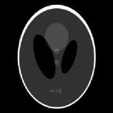
For the piecewise constant phantom experiments, we first compute the fully sampled k-space data using Eq. 3.1 with a piecewise constant function model Eq. 3.6. More precisely, given that ’s are ellipses, Eq. 3.6 can be explicitly written as
| (4.6) |
where ’s are diagonal matrices, ’s are rotation matrices, and is the unit disk. Following [33], we can compute the Fourier transform of Eq. 4.6 by noting that
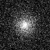
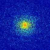
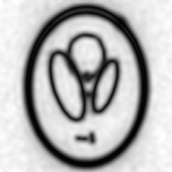
where is the first kind Bessel’s function of order . Then using the variable density random sampling method in [46], we generate undersampled k-space data. The complex white Gaussian noise is also added so that the resulting SNR of the samples is approximately (See Fig. 3).

| Indices | Zero fill | TV Eq. 4.1 | Haar Eq. 4.2 | TLMRI Eq. 3.24 | GIRAF Eq. 4.3 | DDTF Eq. 3.21 | ||
| SNR | 26.66 | |||||||
| HFEN | 0.0572 | |||||||
| NIters | MaxIter | |||||||
| Time() | ||||||||
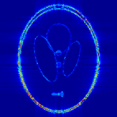
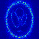
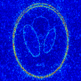
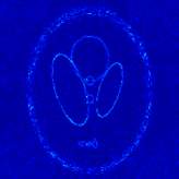
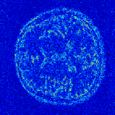
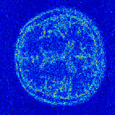
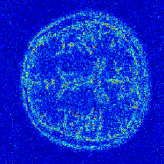
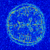
Fig. 4 displays the edges estimated by the proposed model Eq. 3.21. More precisely, using the obtained filter banks at convergence, we compute defined as Eq. 3.23, by varying the rank cutoff , respectively. Here, is the ground truth rank cutoff described in [48]. At first glance, we can see that as the rank cutoff in Eq. 3.23 decreases, the image of contains less artifacts. Most importantly, we can further observe that in any case, is close to near the edges. This demonstrates that the data driven tight frame filter banks used in the proposed model Eq. 3.21 are indeed related to the annihilating filter, as they are also able to estimate the edges of the piecewise constant function via Eq. 3.23. Therefore, we conclude that the proposed sparse regularization via data driven tight frame provides another relaxation of the low rank two-fold Hankel matrix completion based on the annihilating filter.
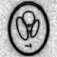
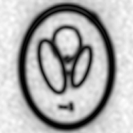
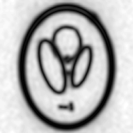
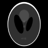
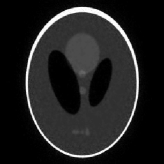
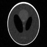
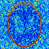
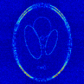
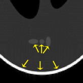
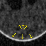
Table 2 summarizes the SNR and the HFEN of the aforementioned restoration models, and Fig. 5 displays the visual comparisons with the zoom-in views in Fig. 8 and the error maps in Fig. 6, respectively. We can see that the proposed data driven tight frame model Eq. 3.21 consistently outperforms both the on-the-grid approaches (Eqs. 4.1, 4.2 and 3.24) and the existing off-the-grid approaches Eq. 4.3 with a smaller error map. Noting that Eq. 3.21 is an off-the-grid approach, the experimental results also suggest that the off-the-grid approaches have better performance in the CS-MRI due to its ability to reducing the basis mismatch between the true support (or the true singularity) in continuum and the discrete grid. In fact, due to this basis mismatch, we can see from Figs. 5c, 5d, 8c and 8d that the on-the-grid approaches lead to the distortions of three small ellipses, and the errors concentrate on the edges (Figs. 6c and 6d) compared to the off-the-grid approaches. Even though Eq. 3.24 is able to restore the three small ellipses, the restored image is still overly smoothed compared to the proposed model with errors concentrated near the edges, as we can see from Figs. 6e and 8e.
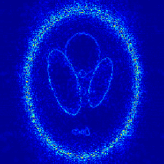
It is also worth noting that among the off-the-grid approaches, the proposed DDTF model introduces less artifacts near the edges. In the literature, the noise in the k-space data affects even in the fully sampled case as the weight matrix amplifies the noise in the high frequencies. Hence under such an amplified noise, it is likely that the direct rank minimization leads to the artifacts near the edges corresponding to the high frequencies in the frequency domain, as shown in Figs. 5f, 5g, 5h, 8f, 8g, 8h, 6f, 6g and 6h. In contrast, the sparse approximation of can achieve the denoising effect in spite of the amplified noise, leading to the better restoration results with less artifacts near the edges.
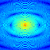
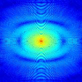
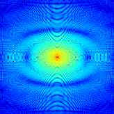
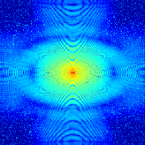
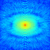
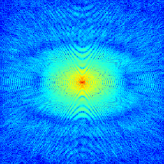
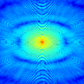
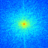
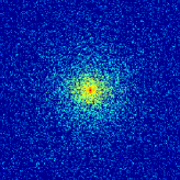
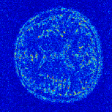
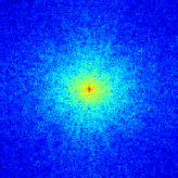
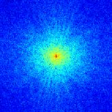
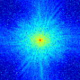
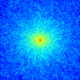
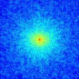
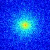
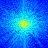
For further comparisons, we also present the restored k-space data (in the log scale) in Fig. 7. Note that since the sampling is dense in the low frequencies while the high frequencies are loosely sampled, the restoration qualities depend heavily on the restoration accuracy of high frequency k-space data. Indeed, we can see from Figs. 7c, 7d and 7e that the restored k-space data by Eqs. 4.1, 4.2 and 3.24 decays faster than the original one, which also leads to the inferior restoration results. Even though the GIRAF models are in general able to restore the high frequency part better than the on-the-grid approaches, they still fail to restore the dominant structures on the high frequencies, as shown in Figs. 7f, 7g and 7h. In contrast, the proposed model Eq. 3.21 is able to restore the high frequency k-space data in spite of the loose sampling, which also results in the improvements over the existing approaches. In summary, our proposed DDTF CS-MRI model shows the overall better restoration quality in both the indices (SNR and HFEN) and the visual quality.
Finally, we note that even though Eq. 3.21 requires more iterations than Eq. 4.3 for convergence, the number of iterations is less than Eqs. 4.1, 4.2 and 3.24. We also note that the BCD algorithm of Eq. 3.24 fails to meet the stopping criterion. It is likely that due to the subsequence convergence, the BCD algorithm for Eq. 3.24 behaves inferior to other models, whose algorithms guarantee the global convergence. Moreover, it takes Eq. 3.24 approximately to perform iterations. It is most likely that the generation of patch and the projection of a coefficient matrix onto the ball are most time consuming, affecting the CPU time. Meanwhile, despite the superior restoration performance, it takes Eq. 3.21 approximately to meet the stopping criterion due to a number of discrete convolutions. Even though this is shorter than Eq. 3.24, the proposed approach is still time-consuming compared to Eqs. 4.1, 4.2 and 4.3. Nevertheless, our approach is able to gain on the quality of the restored image.


4.2 Real MR image experiments
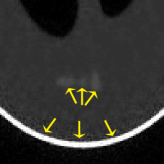
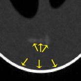
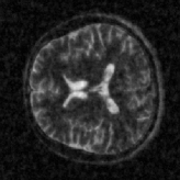
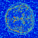
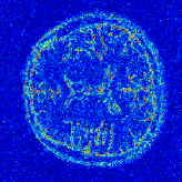
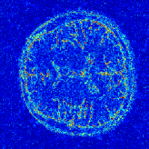
The real MR image experiments use the k-space data which is obtained from a fully sampled -coil acquisition, and then compressed into a single virtual coil using the SVD technique in [72]. Since the data from the single virtual coil is complex-valued in the image domain with smoothly varying phase, we further correct the phase using the method described in [51]. More concretely, we first perform the inverse DFT of the zero padded k-space data, canceling out the phase in the image domain, and passing back to the frequency domain. Then as in the phantom experiments, we generate undersampled k-space data using the variable density sampling, and further add the complex white Gaussian noise so that the resulting SNR of the samples is approximately ; see Fig. 9.


| Indices | Zero fill | TV Eq. 4.1 | Haar Eq. 4.2 | TLMRI Eq. 3.24 | GIRAF Eq. 4.3 | DDTF Eq. 3.21 | ||
| SNR | 16.36 | |||||||
| HFEN | 0.2141 | |||||||
| NIters | MaxIter | |||||||
| Time() | ||||||||
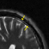
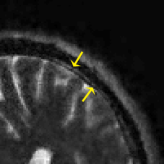
Table 3 summarizes the SNR, the HFEN, the number of iterations and the CPU time of the restoration results. For visual comparisons, the restored images, the error maps, the restored k-space data, and the zoom-in views are presented in Figs. 10, 12, 11 and 13, respectively. We can observe that our proposed model Eq. 3.21 outperforms Eqs. 4.1, 4.2 and 4.3 as in the phantom experiment, but Eq. 3.24 performs slightly better than Eq. 3.21 in the real MR experiment. Nonetheless, the difference of SNR between Eqs. 3.21 and 3.24 is , and visually they appear nearly indistinguishable, as shown in Figs. 10e, 10i, 13e and 13i. In addition, even though our approach is relatively time-consuming (approximately and ) compared to Eqs. 4.1, 4.2 and 4.3, its CPU time is far shorter than Eq. 3.24 which spends but fails to meet stopping criterion. Hence, we can conclude that our proposed approach Eq. 3.21 performs at least comparably to the TLMRI model Eq. 3.24 with shorter computational times than Eq. 3.24.
Finally, we observe that Eq. 3.21 for the real MR experiment requires iterations to meet the stopping criterion, which is more than the piecewise constant phantom image, as shown in Tables 2 and 3. It should be noted that the original k-space data originally contains the thermal noise. It is also possible that compressing a multi coil k-space data into a virtual single coil data generates an error in the k-space data. In any case, it might fail to meet the underlying assumption of the proposed model; the fully sampled k-space data to be restored is modeled by Eq. 3.1 with the piecewise constant proton density in Eq. 3.6. In fact, since the proposed data driven tight frame based approach is a relaxation of a low rank (two-fold) Hankel matrix completion, the future work will require the analysis on the convergence rate of Algorithm 1, which is likely to depend on the incoherence bound (e.g. [17]) of the two-fold Hankel matrix constructed by the original k-space data.


5 Conclusion and future directions
In this paper, we propose a new off-the-grid regularization based CS-MRI reconstruction model for the piecewise constant image restoration in the two dimensional FRI framework [51][51]. Our proposed model is inspired by the observation that the SVD of a Hankel matrix to some extent corresponds to an adaptive tight frame system which can sparsely represent a given image. This motivates us to adopt the sparse approximation by the data driven tight frames as an alternative to the structured low rank matrix completion. Finally, the numerical experiments show that our approach outperforms both the conventional on-the-grid approaches and the existing the low rank Hankel matrix models and their relaxations.
For the future work, we plan to provide a rigorous theoretical framework on our observations. Specifically, we need to rigorously analyze whether the data driven tight frame can indeed reflect the true frequency information of spectrally sparse signals (Such signals correspond to low rank Hankel matrices). In addition to the analysis on the data driven tight frame, we also need to analyze the relation between the convergence rate of Algorithm 1 and the incoherence bound of the underlying original k-space data. It would be also interesting to find other pseudodifferential operators/Fourier integral operators which can provide more insightful information on the rank of the structured matrix constructed from the Fourier transform of a piecewise constant function. For example, we can attempt to find transformations under which the rank of the structured matrix is related to in Eq. 3.6.
Finally, to broaden the scope of applications, it is also likely to extend the idea in this paper to 1) the piecewise smooth image restoration framework, such as the total generalized variation model [10] and the combined first and second order TV model [6, 54], by considering the higher order derivatives; 2) the “blind” multi-coil CS-MRI reconstruction task, whose inverse problem corresponds to a multi-channel blind deconvolution problem with the unknown coil sensitivity map. For the blind multi-coil CS-MRI reconstruction, even though it is not clear for us at this moment how to extend our approach, this is nevertheless definitely a future direction we would like to work on. Motivated by the recent works on the deep learning techniques combined with the structured low rank matrix approaches [38, 41, 55, 56], we are also interested in developing a deep learning framework based on our approach.
Appendix A Proof of Theorem 3.2
Let be a piecewise constant function defined as Eq. 3.6 and . Assume that , and consider its full SVD
| (A.3) |
with and for . Consider by reformulating in Eq. A.3 into a filter supported on . We note that
| (A.4) |
Taking summation along the diagonal and rearranging into the two dimensional multi-indices, we can write Eq. A.4 as
Hence, and in Eqs. 3.16 and 3.17 defined by using these satisfies
which shows that the filters form a tight frame system.
To complete the proof, we note that
where is performed by reformulating into a filter. Then Eq. A.3 implies that for we have
This completes the proof.
Acknowledgments
The authors would like to thank Dr. Greg Ongie in the Department of Statistics at the University of Chicago, an author of [48, 50, 51, 52], for making the data sets as well as the MATLAB toolbox available so that the experiments can be implemented. The authors also thank the anonymous reviewers for their constructive suggestions and comments that helped tremendously with improving the presentation of this paper.
References
- [1] M. Aharon, M. Elad, and A. Bruckstein, -SVD: an algorithm for designing overcomplete dictionaries for sparse representation, IEEE Trans. Signal Process., 54 (2006), pp. 4311–4322, https://doi.org/10.1109/TSP.2006.881199.
- [2] H. Attouch, J. Bolte, P. Redont, and A. Soubeyran, Proximal alternating minimization and projection methods for nonconvex problems: an approach based on the Kurdyka-Lojasiewicz inequality, Math. Oper. Res., 35 (2010), pp. 438–457, https://doi.org/10.1287/moor.1100.0449.
- [3] C. Bao, J. Cai, and H. Ji, Fast sparsity-based orthogonal dictionary learning for image restoration, in 2013 IEEE International Conference on Computer Vision, Dec 2013, pp. 3384–3391, https://doi.org/10.1109/ICCV.2013.420.
- [4] C. Bao, H. Ji, Y. Quan, and Z. Shen, Dictionary learning for sparse coding: algorithms and convergence analysis, IEEE Trans. Pattern Anal. Mach. Intell., 38 (2016), pp. 1356–1369, https://doi.org/10.1109/TPAMI.2015.2487966.
- [5] C. Bao, H. Ji, and Z. Shen, Convergence analysis for iterative data-driven tight frame construction scheme, Appl. Comput. Harmon. Anal., 38 (2015), pp. 510–523, https://doi.org/10.1016/j.acha.2014.06.007.
- [6] M. Bergounioux and L. Piffet, A second-order model for image denoising, Set-Valued Var. Anal., 18 (2010), pp. 277–306, https://doi.org/10.1007/s11228-010-0156-6.
- [7] B. N. Bhaskar, G. Tang, and B. Recht, Atomic norm denoising with applications to line spectral estimation, IEEE Trans. Signal Process., 61 (2013), pp. 5987–5999, https://doi.org/10.1109/TSP.2013.2273443.
- [8] T. Blu, P. Dragott, M. Vetterli, P. Marziliano, and L. Coulot, Sparse sampling of signal innovations, IEEE Signal Process. Mag., 25 (2008), pp. 31–40, https://doi.org/10.1109/MSP.2007.914998.
- [9] J. Bolte, S. Sabach, and M. Teboulle, Proximal alternating linearized minimization for nonconvex and nonsmooth problems, Math. Program., 146 (2014), pp. 459–494, https://doi.org/10.1007/s10107-013-0701-9.
- [10] K. Bredies, K. Kunisch, and T. Pock, Total generalized variation, SIAM J. Imaging Sci., 3 (2010), pp. 492–526, https://doi.org/10.1137/090769521.
- [11] J. F. Cai, R. H. Chan, and Z. Shen, A framelet-based image inpainting algorithm, Appl. Comput. Harmon. Anal., 24 (2008), pp. 131–149, https://doi.org/10.1016/j.acha.2007.10.002.
- [12] J. F. Cai, B. Dong, S. Osher, and Z. Shen, Image restoration: total variation, wavelet frames, and beyond, J. Amer. Math. Soc., 25 (2012), pp. 1033–1089, https://doi.org/10.1090/S0894-0347-2012-00740-1.
- [13] J. F. Cai, H. Ji, Z. Shen, and G. B. Ye, Data-driven tight frame construction and image denoising, Appl. Comput. Harmon. Anal., 37 (2014), pp. 89–105, https://doi.org/10.1016/j.acha.2013.10.001.
- [14] J. F. Cai, S. Osher, and Z. Shen, Split Bregman methods and frame based image restoration, Multiscale Model. Simul., 8 (2009/10), pp. 337–369, https://doi.org/10.1137/090753504.
- [15] J. F. Cai, X. Qu, W. Xu, and G. B. Ye, Robust recovery of complex exponential signals from random Gaussian projections via low rank Hankel matrix reconstruction, Appl. Comput. Harmon. Anal., 41 (2016), pp. 470–490, https://doi.org/10.1016/j.acha.2016.02.003.
- [16] J. F. Cai, T. Wang, and K. Wei, Spectral compressed sensing via projected gradient descent, SIAM J. Optim., 28 (2018), pp. 2625–2653, https://doi.org/10.1137/17M1141394.
- [17] J. F. Cai, T. Wang, and K. Wei, Fast and provable algorithms for spectrally sparse signal reconstruction via low-rank Hankel matrix completion, Appl. Comput. Harmon. Anal., 46 (2019), pp. 94–121, https://doi.org/10.1016/j.acha.2017.04.004.
- [18] E. J. Candès and C. Fernandez-Granda, Super-resolution from noisy data, J. Fourier Anal. Appl., 19 (2013), pp. 1229–1254, https://doi.org/10.1007/s00041-013-9292-3.
- [19] E. J. Candès and C. Fernandez-Granda, Towards a mathematical theory of super-resolution, Comm. Pure Appl. Math., 67 (2014), pp. 906–956, https://doi.org/10.1002/cpa.21455.
- [20] E. J. Candès and B. Recht, Exact matrix completion via convex optimization, Found. Comput. Math., 9 (2009), pp. 717–772, https://doi.org/10.1007/s10208-009-9045-5.
- [21] E. J. Candès, J. Romberg, and T. Tao, Robust uncertainty principles: exact signal reconstruction from highly incomplete frequency information, IEEE Trans. Inform. Theory, 52 (2006), pp. 489–509, https://doi.org/10.1109/TIT.2005.862083.
- [22] R. H. Chan, T. F. Chan, L. Shen, and Z. Shen, Wavelet algorithms for high-resolution image reconstruction, SIAM J. Sci. Comput., 24 (2003), pp. 1408–1432, https://doi.org/10.1137/S1064827500383123.
- [23] Y. Chen and Y. Chi, Robust spectral compressed sensing via structured matrix completion, IEEE Trans. Inform. Theory, 60 (2014), pp. 6576–6601, https://doi.org/10.1109/TIT.2014.2343623.
- [24] Y. Chi, A. Pezeshki, L. Scharf, and R. Calderbank, Sensitivity to basis mismatch in compressed sensing, in 2010 IEEE International Conference on Acoustics, Speech and Signal Processing, March 2010, pp. 3930–3933, https://doi.org/10.1109/ICASSP.2010.5495800.
- [25] J. K. Choi, C. Bao, and X. Zhang, PET-MRI joint reconstruction by joint sparsity based tight frame regularization, SIAM J. Imaging Sci., 11 (2018), pp. 1179–1204, https://doi.org/10.1137/17M1131453.
- [26] B. Dong and Z. Shen, MRA-based wavelet frames and applications, in Mathematics in Image Processing, vol. 19 of IAS/Park City Math. Ser., Amer. Math. Soc., Providence, RI, 2013, pp. 9–158.
- [27] B. Dong and Z. Shen, Image restoration: a data-driven perspective, in Proceedings of the 8th International Congress on Industrial and Applied Mathematics, Higher Ed. Press, Beijing, 2015, pp. 65–108.
- [28] D. L. Donoho, Compressed sensing, IEEE Trans. Inform. Theory., 52 (2006), pp. 1289–1306, https://doi.org/10.1109/TIT.2006.871582.
- [29] M. Fazel, T. K. Pong, D. Sun, and P. Tseng, Hankel matrix rank minimization with applications to system identification and realization, SIAM J. Matrix Anal. Appl., 34 (2013), pp. 946–977, https://doi.org/10.1137/110853996.
- [30] G. B. Folland, Real Analysis: Modern Techniques and Their Applications, Pure and Appl. Math., John Wiley & Sons Inc., New York, 2nd ed., 1999.
- [31] M. Fornasier, H. H. Rauhut, and R. Ward, Low-rank matrix recovery via iteratively reweighted least squares minimization, SIAM J. Optim., 21 (2011), pp. 1614–1640, https://doi.org/10.1137/100811404.
- [32] T. Goldstein and S. J. Osher, The split Bregman method for -regularized problems, SIAM J. Imaging Sci., 2 (2009), pp. 323–343, https://doi.org/10.1137/080725891.
- [33] M. Guerquin-Kern, L. Lejeune, K. P. Pruessmann, and M. Unser, Realistic analytical phantoms for parallel magnetic resonance imaging, IEEE Trans. Med. Imag., 31 (2012), pp. 626–636, https://doi.org/10.1109/TMI.2011.2174158.
- [34] E. M. Haacke, R. W. Brown, M. R. Thompson, and R. Venkatesan, Magnetic Resonance Imaging : Physical Principles and Sequence Design, Wiley, 1st ed., June 1999.
- [35] J. P. Haldar, Low-rank modeling of local -space neighborhoods (loraks) for constrained MRI, IEEE Trans. Med. Imag., 33 (2014), pp. 668–681, https://doi.org/10.1109/TMI.2013.2293974.
- [36] B. Han, G. Kutyniok, and Z. Shen, Adaptive multiresolution analysis structures and shearlet systems, SIAM J. Numer. Anal., 49 (2011), pp. 1921–1946, https://doi.org/10.1137/090780912.
- [37] C. M. Hyun, H. P. Kim, S. M. Lee, S. Lee, and J. K. Seo, Deep learning for undersampled MRI reconstruction, Phys. Med. Biol., 63 (2018), p. 135007, https://doi.org/10.1088/1361-6560/aac71a.
- [38] M. Jacob, M. P. Mani, and J. C. Ye, Structured low-rank algorithms: theory, MR applications, and links to machine learning, arXiv preprint, (2019), https://arXiv:1910.12162.
- [39] K. H. Jin, D. Lee, and J. C. Ye, A general framework for compressed sensing and parallel MRI using annihilating filter based low-rank Hankel matrix, IEEE Trans. Comput. Imag., 2 (2016), pp. 480–495, https://doi.org/10.1109/TCI.2016.2601296.
- [40] K. H. Jin, J. Y. Um, D. Lee, J. Lee, S. H. Park, and J. C. Ye, MRI artifact correction using sparselow-rank decomposition of annihilating filter-based hankel matrix, Magn. Reson. Med., 78 (2017), pp. 327–340, https://doi.org/10.1002/mrm.26330, https://arxiv.org/abs/https://onlinelibrary.wiley.com/doi/pdf/10.1002/mrm.26330.
- [41] T. H. Kim and J. P. Haldar, Learning-based computational MRI reconstruction without big data: from linear interpolation and structured low-rank matrices to recurrent neural networks, in Wavelets and Sparsity XVIII, D. V. D. Ville, M. Papadakis, and Y. M. Lu, eds., vol. 11138, International Society for Optics and Photonics, SPIE, 2019, pp. 346 – 352, https://doi.org/10.1117/12.2527584.
- [42] K. Kurdyka, On gradients of functions definable in o-minimal structures, Ann. Inst. Fourier (Grenoble), 48 (1998), pp. 769–783, http://www.numdam.org/item?id=AIF_1998__48_3_769_0.
- [43] Y. Liu, J. F. Cai, Z. Zhan, D. Guo, J. Ye, Z. Chen, and X. Qu, Balanced sparse model for tight frames in compressed sensing magnetic resonance imaging, PLOS ONE, 10 (2015), pp. 1–19, https://doi.org/10.1371/journal.pone.0119584.
- [44] S. Lojasiewicz, On semi-analytic and subanalytic geometry, in Panoramas of Mathematics (Warsaw, 1992/1994), vol. 34 of Banach Center Publ., Polish Acad. Sci. Inst. Math., Warsaw, 1995, pp. 89–104.
- [45] L. Lu, W. Xu, and S. Qiao, A fast SVD for multilevel block Hankel matrices with minimal memory storage, Numer. Algorithms, 69 (2015), pp. 875–891, https://doi.org/10.1007/s11075-014-9930-0.
- [46] M. Lustig, D. Donoho, and J. M. Pauly, Sparse MRI: the application of compressed sensing for rapid MR imaging, Magn. Reson. Med., 58 (2007), pp. 1182–1195, https://doi.org/10.1002/mrm.21391.
- [47] K. Mohan and M. Fazel, Iterative reweighted algorithms for matrix rank minimization, J. Mach. Learn. Res., 13 (2012), pp. 3441–3473.
- [48] G. Ongie, S. Biswas, and M. Jacob, Convex recovery of continuous domain piecewise constant images from nonuniform Fourier samples, IEEE Trans. Signal Process., 66 (2018), pp. 236–250, https://doi.org/10.1109/TSP.2017.2750111.
- [49] G. Ongie and M. Jacob, Recovery of piecewise smooth images from few fourier samples, in 2015 International Conference on Sampling Theory and Applications (SampTA), May 2015, pp. 543–547, https://doi.org/10.1109/SAMPTA.2015.7148950.
- [50] G. Ongie and M. Jacob, Super-resolution MRI using finite rate of innovation curves, in 2015 IEEE 12th International Symposium on Biomedical Imaging (ISBI), April 2015, pp. 1248–1251, https://doi.org/10.1109/ISBI.2015.7164100.
- [51] G. Ongie and M. Jacob, Off-the-grid recovery of piecewise constant images from few Fourier samples, SIAM J. Imaging Sci., 9 (2016), pp. 1004–1041, https://doi.org/10.1137/15M1042280.
- [52] G. Ongie and M. Jacob, A fast algorithm for convolutional structured low-rank matrix recovery, IEEE Trans. Comput. Imag., 3 (2017), pp. 535–550, https://doi.org/10.1109/TCI.2017.2721819.
- [53] H. Pan, T. Blu, and P. L. Dragotti, Sampling curves with finite rate of innovation, IEEE Trans. Signal Process., 62 (2014), pp. 458–471, https://doi.org/10.1109/TSP.2013.2292033.
- [54] K. Papafitsoros and C. B. Schönlieb, A combined first and second order variational approach for image reconstruction, J. Math. Imaging Vision, 48 (2014), pp. 308–338, https://doi.org/10.1007/s10851-013-0445-4.
- [55] A. Pramanik, H. Aggarwal, and M. Jacob, Deep generalization of structured low-rank algorithms (Deep-SLR), arXiv preprint, (2019), https://arXiv:1912.03433.
- [56] A. Pramanik, H. Aggarwal, and M. Jacob, Off-the-grid model based deep learning (O-Modl), in 2019 IEEE 16th International Symposium on Biomedical Imaging (ISBI 2019), April 2019, pp. 1395–1398, https://doi.org/10.1109/ISBI.2019.8759403.
- [57] K. P. Pruessmann, M. Weiger, M. B. Scheidegger, and P. Boesiger, SENSE: sensitivity encoding for fast MRI, Magn. Reson. Med., 42 (1999), pp. 952–962, https://doi.org/10.1002/(SICI)1522-2594(199911)42:5<952::AID-MRM16>3.0.CO;2-S.
- [58] S. Ravishankar and Y. Bresler, Mr image reconstruction from highly undersampled k-space data by dictionary learning, IEEE Trans. Med. Imag., 30 (2011), pp. 1028–1041, https://doi.org/10.1109/TMI.2010.2090538.
- [59] S. Ravishankar and Y. Bresler, Learning sparsifying transforms, IEEE Trans. Signal Process., 61 (2013), pp. 1072–1086, https://doi.org/10.1109/TSP.2012.2226449.
- [60] S. Ravishankar and Y. Bresler, Efficient blind compressed sensing using sparsifying transforms with convergence guarantees and application to magnetic resonance imaging, SIAM J. Imaging Sci., 8 (2015), pp. 2519–2557, https://doi.org/10.1137/141002293.
- [61] E. V. Reeth, I. W. K. Tham, C. H. Tan, and C. L. Poh, Super-resolution in magnetic resonance imaging: A review, Concept. Magn. Reson. A, 40A (2012), pp. 306–325, https://doi.org/10.1002/cmr.a.21249.
- [62] A. Ron and Z. Shen, Affine systems in : the analysis of the analysis operator, J. Funct. Anal., 148 (1997), pp. 408–447, https://doi.org/10.1006/jfan.1996.3079.
- [63] Z. Shen, Wavelet frames and image restorations, in Proceedings of the International Congress of Mathematicians. Volume IV, Hindustan Book Agency, New Delhi, 2010, pp. 2834–2863.
- [64] M. Vetterli, P. Marziliano, and T. Blu, Sampling signals with finite rate of innovation, IEEE Trans. Signal Process., 50 (2002), pp. 1417–1428, https://doi.org/10.1109/TSP.2002.1003065.
- [65] J. Wang and J. F. Cai, Data-driven tight frame for multi-channel images and its application to joint color-cepth image reconstruction, J. Oper. Res. Soc. China, 3 (2015), pp. 99–115, https://doi.org/10.1007/s40305-015-0074-2.
- [66] B. Wen, S. Ravishankar, and Y. Bresler, FRIST-flipping and rotation invariant sparsifying transform learning and applications, Inverse Problems, 33 (2017), p. 074007, https://doi.org/10.1088/1361-6420/aa6c6e.
- [67] W. Xu, J. Cai, K. V. Mishra, M. Cho, and A. Kruger, Precise semidefinite programming formulation of atomic norm minimization for recovering -dimensional () off-the-grid frequencies, in 2014 Information Theory and Applications Workshop (ITA), Feb 2014, pp. 1–4, https://doi.org/10.1109/ITA.2014.6804267.
- [68] Y. Xu and W. Yin, A block coordinate descent method for regularized multiconvex optimization with applications to nonnegative tensor factorization and completion, SIAM J. Imaging Sci., 6 (2013), pp. 1758–1789, https://doi.org/10.1137/120887795.
- [69] J. C. Ye, J. M. Kim, K. H. Jin, and K. Lee, Compressive sampling using annihilating filter-based low-rank interpolation, IEEE Trans. Inform. Theory, 63 (2017), pp. 777–801, https://doi.org/10.1109/TIT.2016.2629078.
- [70] J. Ying, H. Lu, Q. Wei, J. F. Cai, D. Guo, J. Wu, Z. Chen, and X. Qu, Hankel matrix nuclear norm regularized tensor completion for -dimensional exponential signals, IEEE Trans. Signal Process., 65 (2017), pp. 3702–3717, https://doi.org/10.1109/TSP.2017.2695566.
- [71] R. Zhan and B. Dong, CT image reconstruction by spatial-Radon domain data-driven tight frame regularization, SIAM J. Imaging Sci., 9 (2016), pp. 1063–1083, https://doi.org/10.1137/16M105928X.
- [72] T. Zhang, J. M. Pauly, S. S. Vasanawala, and M. Lustig, Coil compression for accelerated imaging with cartesian sampling, Magn. Reson. Med., 69 (2013), pp. 571–582, https://doi.org/10.1002/mrm.24267, https://arxiv.org/abs/https://onlinelibrary.wiley.com/doi/pdf/10.1002/mrm.24267.