A Cooperative Coordination Solver for Travelling Thief Problems

Abstract

The travelling thief problem (TTP) is a representative of multi-component optimisation problems where the components interact with each other. TTP combines two interdependent components: the knapsack problem (KP) and the travelling salesman problem (TSP). A thief performs a cyclic tour through a set of cities, and pursuant to a collection plan, collects a subset of items into a rented knapsack with finite capacity. The aim is to maximise overall profit while minimising renting cost. Existing TTP solvers typically solve the KP and TSP components in an interleaved manner, where the solution of one component is kept fixed while the solution of the other component is modified. This suggests low coordination between solving the two components, possibly leading to low-quality TTP solutions. The 2-OPT heuristic is often used for solving the TSP component, which reverses a segment in the cyclic tour. Within the TTP context, 2-OPT does not take into account the collection plan, which can result in a lower objective value. This in turn can result in the tour modification to be rejected by a solver. To address this issue, we propose an expanded form of 2-OPT in order to change the collection plan in coordination with modifying the tour. Items regarded as less profitable and collected in cities located earlier in the reversed segment are substituted by items that tend to be more profitable and not collected in cities located later in the reversed segment. The collection plan is further changed through a modified form of the hill-climbing bit-flip search, where changes in the collection state are only permitted for boundary items, which are defined as lowest profitable collected items or highest profitable uncollected items. This restriction reduces the amount of time spent on the KP component, thereby allowing more tours to be evaluated by the TSP component within a given time budget. The two proposed approaches form the basis of a new cooperative coordination solver, which finds a large number of new best gain values and outperforms several state-of-the-art TTP solvers on a comprehensive set of benchmark TTP instances.

Keywords: multi-component optimisation; interdependent components; combinatorial optimisation; travelling thief problem; travelling salesman problem; knapsack problem.

1 Introduction

Practical constraint optimisation problems [2] often consist of several interdependent components [3]. Finding an optimal overall solution to such problems cannot be guaranteed by simply finding an optimal solution to each underlying component [4, 5, 6]. A representative of such multi-component problems is the travelling thief problem (TTP) [3, 7], which comprises two interdependent NP-hard components: the knapsack problem (KP) [8] and the travelling salesman problem (TSP) [9]. The overall problem is described as follows. A thief performs a cyclic tour through a set of specified cities. The thief collects a subset of obtainable items into a finite capacity knapsack pursuant to a collection plan. The knapsack is rented, so it has an associated cost. As items are collected at each city, the overall weight and profit of the items in the knapsack increase, leading to a decrease in the speed of the thief. This in turn leads to an increase to the overall travelling time and thus the cost of the knapsack. The aim of a TTP solution is to concurrently minimise the renting cost and maximise the overall profit of the collected items. TTP can be thought of as a proxy for many real-world logistics problems [10].

Existing TTP solvers typically use separate modules for solving the KP and TSP components, and follow an interleaved approach: the solution of one component is kept fixed while the solution of the other component is modified [7]. In this context, the aim of solving the KP component is to maximise the overall profit given a fixed cyclic tour, while the aim of solving the TSP component is to minimise the overall travelling time given a fixed collection plan. However, this interleaved approach suggests low coordination between solving the two components, possibly leading to low quality TTP solutions.

The 2-OPT segment reversal heuristic [11] is often employed for solving the TSP component. In the context of TTP, the 2-OPT heuristic does not take into account the collection plan, which can result in a decrease of the TTP objective value. This in turn can result in the tour modification to be rejected by a solver, which suggests that many possible segment reversals can be rejected without considering potential changes to the collection plan. This unnecessarily restricts the search of the TTP solution space.

For solving the KP component, a popular approach is the bit-flip search [7, 12], which is a hill-climber that searches via flipping the collection status (from collected to uncollected and vice-versa) of one item at a time. The downside of this approach is that the small and untargeted change in the collection plan results in a slow and meandering exploration of the solution space. When a time limit is placed for finding a solution, the solution space may not be explored adequately, which can contribute to low quality TTP solutions.

To address the poor coordination between solving the KP and TSP components, we propose a modified and extended version of 2-OPT, in order to explicitly adjust the collection plan in coordination with changes made to the cyclic tour. After reversing the segment, items regarded as less profitable and collected in cities located earlier in the reversed segment are substituted by items that tend to be equally or more profitable and not collected in cities located later in the reversed segment. We term the new heuristic as Profit Guided Coordination Heuristic (PGCH). An early version of the PGCH heuristic, proposed in our preliminary work [1], uses only the sequence of (the profitability ratios of) the lowest profitable collected items to adjust the collection plan. In contrast, the extended version uses both the sequence of the lowest profitable collected items and the sequence of the highest profitable uncollected items to adjust the collection plan, as discussed in more detail in Section 4.

We further extend our preliminary work [1] by proposing a more targeted form of the bit-flip search, termed Boundary Bit-Flip search, where a restriction is placed to only consider changes to the collection state of boundary items. We define two types of boundary items: (i) lowest profitable collected items among all items collected earlier in the segment, and (ii) highest profitable uncollected items among all items not collected later in the segment. The restriction reduces the amount of time spent on the KP component, thereby allowing more tours to be evaluated by the TSP component within a time limit. We combine the proposed PGCH and Boundary Bit-Flip approaches into a new TTP solver, termed as cooperative coordination (CoCo) solver. A comparative evaluation on a comprehensive set of benchmark TTP instances shows that the proposed solver finds a large number of new best gain values and also outperforms several state-of-the-art TTP solvers: MATLS [10], S5 [12], CS2SA* [13] and MEA2P [14].

We continue the paper as follows. Section 2 provides an overview of related work. Section 3 formally defines TTP, the 2-OPT heuristic, the bit-flip operator, and other necessary mathematical details. Section 4 describes the proposed coordination heuristic. Section 5 describes the proposed targeted form of bit-flip search. Section 6 combines the two proposed heuristics into the proposed CoCo solver. Section 7 empirically shows the effects of the proposed heuristics and provides the comparative evaluation. Section 8 summarises the main findings.

2 Related Work

TTP was introduced in [3] with many benchmark instances given in [7]. Existing TTP solvers can be grouped into 5 main categories: (i) constructive methods, (ii) fixed-tour methods, (iii) cooperative methods, (iv) full encoding methods, and (v) hyper-heuristic methods. Each of the categories is briefly overviewed below. For a more thorough treatment, the reader is directed to the recent review of TTP solvers in [15].

In constructive methods, an initial cyclic tour is generated for the TSP component using the classic Chained Lin-Kernighan heuristic [16]. The tour is then kept fixed while the collection plan for the KP component is generated by employing scores assigned to the items based on their weight, profit, and position in the tour. This category includes approaches such as Simple Heuristic [7], Density-based Heuristic [17], Insertion [10] and PackIterative [12]. These approaches are used in restart-based algorithms such as S5 [12] and in the initialisation phase of more elaborate methods.

In fixed-tour methods, after generating an initial cyclic tour as per constructive methods, an iterative improvement heuristic is used to solve the KP component. Two iterative methods for solving the KP component are proposed in [7]: (i) Random Local Search, which is a hill-climbing bit-flip search where the collection status of a randomly selected item is flipped in each iteration, and (ii) (1+1)-EA, a simple evolutionary algorithm where the collection status of a set of randomly selected items is flipped in each iteration.

Cooperative methods are iterative approaches based on co-operational co-evolution [18]. After generating an initial TTP solution using a constructive or fixed-tour method, the KP and TSP components are solved by two separate modules. These two modules are executed by a coordinating agent (or meta-optimiser) in an interleaved form. The coordinating agent combines the two solutions to produce an overall solution, thereby considering the interdependency between the KP and TSP components [15]. Example methods include CoSolver [17], CoSolver with 2-OPT and Simulated Annealing (CS2SA) [19], and CS2SA with offline instance-based parameter tuning (CS2SA*) [13].

In full-encoding methods, the problem is considered as a whole. Example methods include Memetic Algorithm with Two-stage Local Search (MATLS) [10], memetic algorithm with edge-assembly and two-point crossover operators (MEA2P) [14], a swarm intelligence algorithm [20] based on max–min ant system [21], Memetic Algorithm with 2-OPT and Bit-Flip search [19], and Joint 2-OPT and Bit-Flip [22], which changes the collection status of just one item each time a segment in the cyclic tour is reversed.

In hyper-heuristic based methods, genetic programming is used to generate or select low level heuristics for the TSP and/or KP components. In [23], a genetic programming based approach generates two packing heuristics for the KP component. An individual in each generation is a tree whose internal nodes are simple arithmetic operators, while the leaf nodes are the numerical parameters of a given TTP instance. In [24, 25], genetic programming is used to learn how to select a sequence of low level heuristics to address both the KP and TSP components. In [24], an individual in each generation is a Bayesian network in which each node corresponds to a low level heuristic. In [25], an individual in each generation is a tree in which the internal nodes are functions while the leaf nodes correspond to low level heuristics.

3 Background

Each TTP instance is comprised of a set $\{1,\ldots,m\}$ of $m$ items and a set $\{1,\ldots,n\}$ of $n$ cities. The distance between each pair of cities $i\neq i^{\prime}$ is $d(i,i^{\prime})=d(i^{\prime},i)$. Each item $j$ is located at city $l_{j}>1$ (ie., there are no items in the city $1$). Moreover, each item has weight $w_{j}>0$, profit $\pi_{j}>0$, and corresponding profitability ratio $r_{j}=\pi_{j}/w_{j}$. An item $j$ is regarded more profitable than item $j^{\prime}$ if $r_{j}>r_{j^{\prime}}$, or $\pi_{j}>\pi_{j^{\prime}}$ if $r_{j}=r_{j^{\prime}}$.

The thief begins a cyclic tour at city $1$, travels between cities (visiting each city only once), collects a subset of the items available in each city, and returns to city $1$ at the conclusion of the tour. The cyclic tour is represented by using a permutation of $n$ cities. Let us represent a given cyclic tour as $c$, with $c_{k}=i$ indicating that the $k$-th city in the tour $c$ is $i$, and $c(i)=k$ indicating that the position of city $i$ in the tour $c$ is $k$. Here $c_{1}=1$ and $c(1)=1$. A knapsack with a rent rate $R$ per unit time and a weight capacity $W$ is rented by the thief to hold the collected items. A collection plan $p$ indicates that item $j$ is selected for collection if $p_{j}=1$, or not selected if $p_{j}=0$. An overall solution that provides a cyclic tour $c$ and a collection plan $p$ is expressed as $\langle c,p\rangle$.

The combined weight of the items collected from city $i$ is denoted by $W_{p}(i)=\sum_{l_{j}=i}w_{j}p_{j}$. The combined weight of the items collected from the initial $k$ cities in the tour $c$ is denoted by $W_{c,p}(k)=\sum_{k^{\prime}=1}^{k}W_{p}(c_{k^{\prime}})$. The thief traverses from city $c_{k}$ to the next city with speed $v_{c,p}(k)$. The speed decreases as $W_{c,p}(k)$ increases. The speed at the city $c_{k}$ is given by $v_{c,p}(k)=v_{\textrm{max}}-W_{c,p}(k)\times(v_{\textrm{max}}-v_{\textrm{min}})/W$, where $v_{\textrm{min}}$ and $v_{\textrm{max}}$ are the specified minimum and maximum speeds, respectively.

Given an overall solution $\langle c,p\rangle$, the combined profit is $P(p)=\sum_{i=1}^{m}p_{i}\pi_{i}$, the travelling time to city $c_{k}$ is $T_{c,p}(k)=\sum_{k^{\prime}=1}^{k-1}d(c_{k^{\prime}},c_{k^{\prime}+1})/v_{c,p}(k^{\prime})$, and the combined travelling time is $T(c,p)=T_{c,p}(n+1)=T_{c,p}(n)+d(c_{n},c_{1})/v_{c,p}(n)$. The goal of a TTP solution is to maximise the overall gain by maximising the overall profit while at the same time minimising the overall renting cost of the knapsack. More formally, the goal is to maximise the objective function $G(c,p)$, defined as

$$G(c,p)=P(p)-R\times T(c,p)$$ (1)

for any possible configuration of $c$ (cyclic tour) and $p$ (item collection plan).

In a similar manner to the co-operational co-evolution approach [18], where a problem is divided to several sub-problems and each sub-problem is solved by a separate module, TTP is often decomposed to its KP and TSP components [17], with each component solved by a dedicated solver. In solving the TSP component, the collection plan $p$ and hence $W_{p}(i)$ for all cities $1\leq i\leq n$ are considered fixed; the aim is to minimise the combined travelling time $T(c,p)$ over any possible cyclic tour $c$. In solving the KP component, the cyclic tour $c$ and hence $c_{k}$ for all positions $1\leq k\leq n$ are considered fixed; the aim is to maximise $G(c,p)$ over any possible collection plan $p$. To generate an initial solution, either a cyclic tour $c$ is generated by assuming an empty collection plan $p$ [13] (where no item is considered collected), or a collection plan $p$ is generated assuming that all distances between cities are zero at the start [17].

To iteratively solve the TSP component, a segment reversal heuristic known as 2-OPT [11] is often used. The underlying 2-OPT($c,k^{\prime},k^{\prime\prime}$) function is defined as follows. Given a tour $c$ as well as positions $k^{\prime}$ and $k^{\prime\prime}$ (under the constraint of $1<k^{\prime}<k^{\prime\prime}\leq n$), the order of the visited cities between $k^{\prime}$ and $k^{\prime\prime}$ is reversed to obtain a new tour $c^{\prime}$. Here $c^{\prime}_{k^{\prime}+k}=c_{k^{\prime\prime}-k}$ is obtained where $0\leq k\leq k^{\prime\prime}-k^{\prime}$.

To iteratively solve the KP component, the bit-flip operator is often used [7, 12]. We define the flipping function as Flip($p,j$), where given a collection plan $p$ and an item $j$, the collection state $p_{j}$ is flipped from $0$ to $1$ or vice versa to obtain a new collection plan $p^{\prime}$.

To evaluate the effects of each application of 2-OPT($c,k^{\prime},k^{\prime\prime}$) and Flip($p,j$), the corresponding objective functions $G(c^{\prime},p)$ and $G(c,p^{\prime})$ must be recalculated. This necessitates recalculating $W_{c^{\prime},p}(k)$ and $T_{c^{\prime},p}(k+1)$ for all positions $k^{\prime}\leq k\leq k^{\prime\prime}$ in 2-OPT($c,k^{\prime},k^{\prime\prime}$), as well as $W_{c,p^{\prime}}(k)$ and $T_{c,p^{\prime}}(k+1)$ for all positions $l_{j}\leq k\leq n$ in Flip($p,j$). This results in an overall computation cost of $\mathcal{O}(n)$ for $G(c^{\prime},p)$ and $G(c,p^{\prime})$.

In the following sections, we use two functions on sequences of numbers called prefix-minimum and postfix-maximum. For any position $k$ of a sequence of $n$ numbers $S=\langle S(1),S(2),...,S(n)\rangle$, the prefix-minimum function is defined as:

$$\Pi(S,k)=\min(\Pi(S,k-1),S(k))$$ (2)

where $\Pi(S,1)=S(1)$. The postfix-maximum function is defined as:

$$\Omega(S,k)=\max(S(k),\Omega(S,k+1))$$ (3)

where $\Omega(S,n)=S(n)$. In other words, the prefix-minimum function returns the smallest number among the first $k$ numbers, while the postfix-maximum function returns the largest number among the last $n-k+1$ numbers for each position $k$ in the sequence of numbers $S$. For example, consider the sequence $S=\langle 9,6,8,4,5,7\rangle$. The corresponding sequences generated via the prefix-minimum and postfix-maximum functions are $\Pi(S)=\langle 9,6,6,4,4,4\rangle$ and $\Omega(S)=\langle 9,8,8,7,7,7\rangle$, respectively.

4 Profit Guided Coordination Heuristic

In the definition of TTP given in Section 3, a plan for collecting the items is required. The items are scattered across the cities, with the collection order necessarily limited by the order of the cities in the cyclic tour. This suggests that in a TTP solution, monotonous ordering of item collection should not be expected. Constructive methods such as PackIterative [12] and Insertion [10] use profitability ratios of the items in conjunction with the distances of the respective cities from the end of the tour. However, in iterative methods which change the order of the cities in solving the TSP component, corresponding changes are required to the collection plan.

As mentioned in Section 3, the 2-OPT segment reversal heuristic is often employed for solving the TSP component. As the length of the segment to be reversed increases, the amount of corresponding changes required for the collection plan is likely to increase. Within the context of a meta-optimiser that interleaves solving the KP and TSP components, the changes to the collection plan are postponed until the dedicated KP solver is executed. However, if a reversed segment is not accepted while solving the TSP component, there is no opportunity to evaluate corresponding changes to the collection plan for the KP component. This unnecessarily restricts the search space, as potentially beneficial combinations of segment reversal with corresponding changes to the collection plan are not even attempted.

As an example, consider the simple TTP instance shown in Figure 1, which has $n=5$ cities and $m=4$ items. Suppose that the capacity of knapsack $W=6$, maximum speed $v_{max}=1$, minimum speed $v_{min}=0.1$ and the renting rate of the knapsack $R=1$. Furthermore, suppose that an interim solution has the cyclic tour $c=[1,2,3,4,5]$ and the collection plan $p=[0,0,1,1]$ (ie., items $3$ and $4$ are collected). The resultant objective value (see Eqn. (1)) for this solution is $G(c,p)=4$. Using the 2-OPT heuristic for reversing the segment $[2,3,4]$ in the cyclic tour $c$, we obtain the candidate cyclic tour $c^{\prime}=[1,4,3,2,5]$. Without changing the collection plan $p$, the corresponding objective value is $G(c^{\prime},p)=-1.5$, which can result in the rejection of the tour modification. However, if the collection plan is fortuitously changed to $p^{\prime}=[1,0,0,1]$, where item $1$ is collected and item $3$ is uncollected, the resultant objective value (gain) is $G(c^{\prime},p^{\prime})=6$. Hence changing the collection plan in coordination with reversing the segment can result in a higher overall gain.

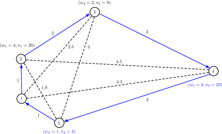
Figure 1: An example TTP instance with 5 cities and 4 items.

To see how to change the collection plan in coordination with segment reversing, let us first examine the solutions found by the PackIterative method (the main building block of the state-of-the-art S5 solver [12]). Using a solution $\langle c,p\rangle$, we consider the lowest profitable item $p(k)$ collected at each city $c_{k}$, as well as the highest profitable item $q(k)$ not collected at city $c_{k}$. We then plot the corresponding sequences of profitability ratios $P_{c,p}(k)=r_{p(k)}$ and $Q_{c,p}(k)=r_{q(k)}$, respectively. If no items are collected at city $c_{k}$, we use the default maximum value of $P_{c,p}(k)=1+\max_{i}r_{i}$, where $\max_{i}r_{i}$ is the maximum $r$ among all the items. Furthermore, if there are no uncollected items at city $c_{k}$, we use default minimum value of $Q_{c,p}(k)=0$.

Figure 2(a) presents the lowest collected and the highest uncollected profitability ratios obtained for the eil76_n750_uncorr_10.ttp benchmark instance (the benchmark instances are described in Section 7). Looking forwards (from the start to the end of the cyclic tour), the discernible trend is a decrease in the lowest collected profitability ratios in the $P_{c,p}$ sequence. Furthermore, looking backwards (from the end to the start of the cyclic tour), the discernible trend is an increase in the highest uncollected profitability ratios in the $Q_{c,p}$ sequence.

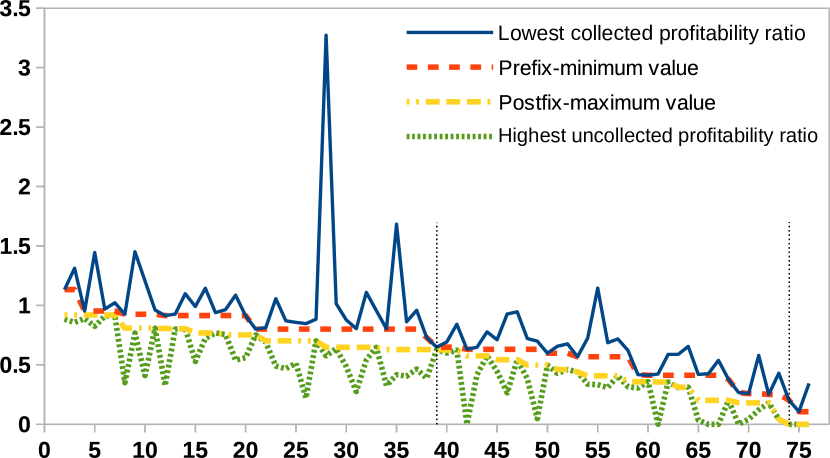
(a)

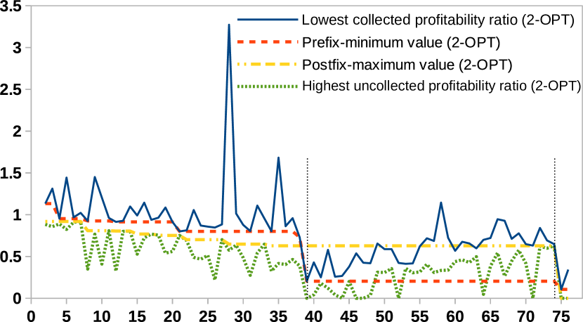
(b)

Figure 2: x-axis: position in a tour; y-axis: profitability ratio. (a): Lowest collected and highest uncollected profitability ratios with the correspondent prefix-minimum and postfix-maximum values in a TTP solution obtained by the PackIterative method for the eil76_n750_uncorr_10.ttp instance, where the overall gain is $77544.88$. (b): Consequence of employing the 2-OPT heuristic, where the segment between positions 39 and 74 is reversed and the collection plan is unchanged, resulting in a lower overall gain of $72151.46$.

To describe the declining trend of the lowest collected profitability ratios in the $P_{c,p}$ sequence looking forwards, we use the prefix-minimum function $\Pi(P_{c,p},k)$ as defined in Eqn. (2), which provides the profitability ratio of the lowest profitable item collected among the first $k$ cities. Furthermore, to describe the rising trend of the highest uncollected profitability ratios in the $Q_{c,p}$ sequence looking backwards, we use the postfix-maximum function $\Omega(Q_{c,p},k)$ as defined in Eqn. (3), which provides the profitability ratio of the highest profitable item not collected among the last $n-k+1$ cities. Figure 2(a) presents the prefix-minimum and postfix-maximum values corresponding to the lowest collected and the highest uncollected profitability ratios, respectively.

Let us employ the 2-OPT heuristic on a segment between positions 39 and 74 of the cyclic tour given in Figure 2(a). The cities between the two positions are reversed, resulting in the tour presented in Figure 2(b). The reversal also results in lower prefix-minimum values and higher postfix-maximum values than the corresponding original prefix-minimum and postfix-maximum values at most positions in the segment. In comparison to the original segment (as well as the entire cyclic tour), in the reversed segment the trend of the lowest collected profitability ratios is rising (looking forwards), and the trend of the highest uncollected profitability ratios is declining (looking backwards). This reversal in trends makes such a 2-OPT move counterproductive and results in a lower overall gain. This may then lead to the move being rejected by a solver due to the lower overall gain. Since the collection plan is not modified, the trade-off between the renting cost and profit is meager for the low profitable items collected from the start of the reversed segment.

We propose to minimise the renting cost of the knapsack and maximise the profit of the collected items by adjusting the collection plan in coordination with reversal of the segment. To achieve this, we propose an extended form of the 2-OPT heuristic, termed as Profit Guided Coordination Heuristic (PGCH). Along with reversing the tour segment, items regarded as less profitable and collected in cities located earlier in the reversed segment are first uncollected. The original prefix-minimum values at the specified tour positions are used as a reference to determine which items must be uncollected. Then, items that tend to be equally or more profitable and not collected in cities located later in the reversed segment are collected. The original postfix-maximum values at the specified tour positions are used as an anchor to determine which items can be collected.

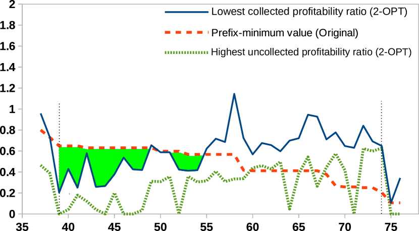
(a)

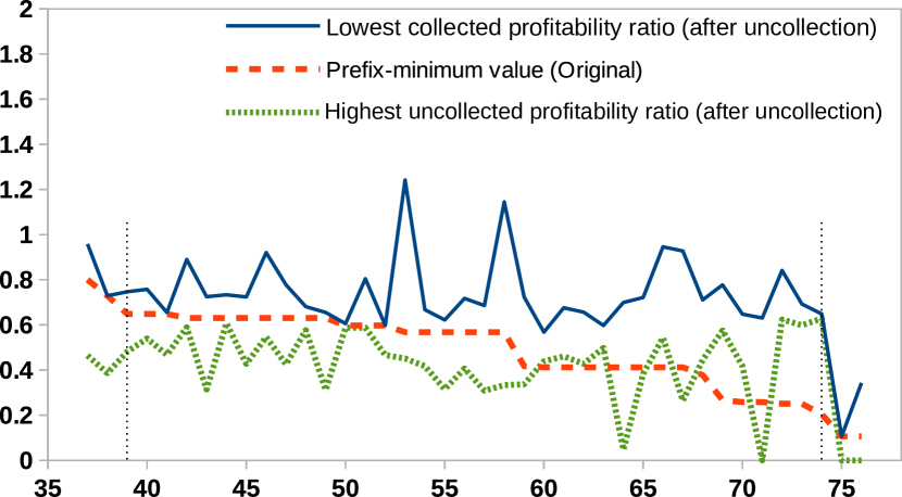
(b)

Figure 3: x-axis: position in a tour; y-axis: profitability ratio. (a): Lowest collected and highest uncollected profitability ratios of the reversed segment from Figure 2(b), with an overlay of original prefix-minimum values (dashed red line) from Figure 2(a). Highlighted green regions under the dashed red line and above the solid blue line indicate the items that must be uncollected. (b): Lowest collected and highest uncollected profitability ratios after uncollecting the items as indicated in (a).

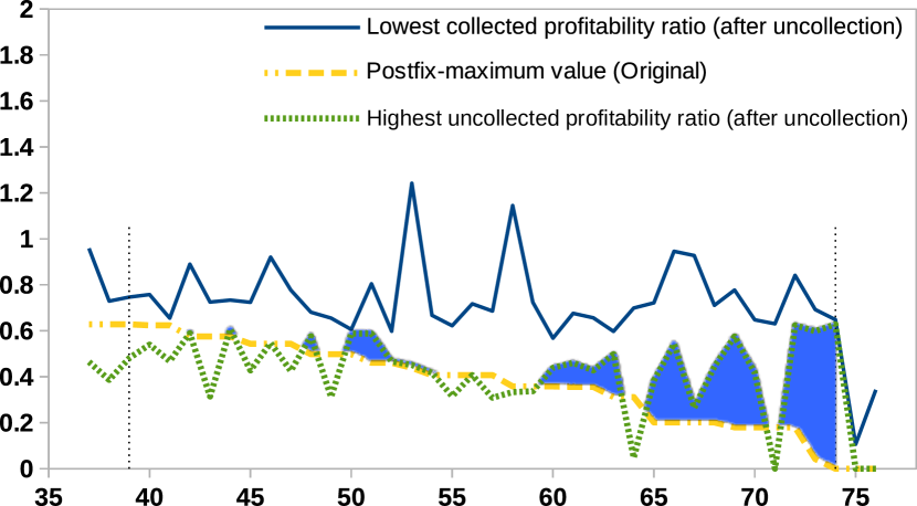
(a)

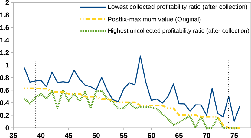
(b)

Figure 4: x-axis: position in a tour; y-axis: profitability ratio. (a): Lowest collected and highest uncollected profitability ratios from Figure 3(b), with an overlay of original postfix-maximum values (dashed yellow line) from Figure 2(a). Highlighted blue regions under the dotted green line and above the dotted-dashed yellow line indicate the items which can be collected. (b): Lowest collected and highest uncollected profitability ratios after collecting most of the items as indicated in (a).

(a)

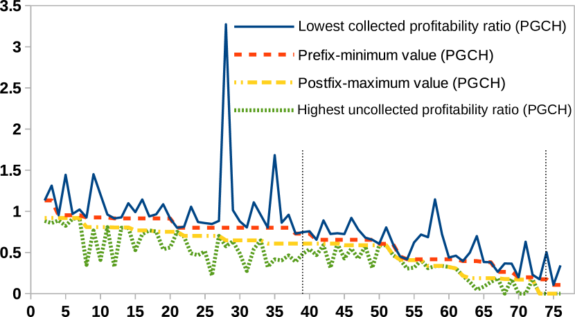
(b)

Figure 5: x-axis: position in a tour; y-axis: profitability ratio. (a): Copy of Figure 2(b), where the 2-OPT heuristic is employed on the segment between positions 39 and 74 of Figure 2(a), resulting in a overall gain of $72151.46$. (b): Consequence of employing PGCH instead of 2-OPT, resulting in an improved overall gain of $78525.18$.

For example, Figure 3(a) shows the lowest collected and the highest uncollected profitability ratios after reversing the segment from Figure 2(b), with an overlay of original prefix-minimum values from Figure 2(a). The highlighted green regions show items which must be uncollected from early positions of the reversed segment. The result of uncollecting the required items is shown in Figure 3(b). Figure 4(a) shows the lowest collected and highest uncollected profitability ratios from Figure 3(b), with an overlay of original postfix-maximum values from Figure 2(a). Highlighted blue regions show items which can be collected from later positions of the reversed segment. The result of collecting most of the items is shown in Figure 4(b). Figure 5 contrasts the effects of the 2-OPT and PGCH moves applied to the segment between positions 39 and 74 in Figure 2(a). The tour modified by PGCH obtains a larger overall gain than both the original tour and the tour modified by 2-OPT.

The formal definition of PGCH($c,p,k^{\prime},k^{\prime\prime}$) used in the preceding example is as follows. Given the positions $k^{\prime}$ and $k^{\prime\prime}$ (where $1<k^{\prime}<k^{\prime\prime}\leq n$) as well as the solution $\langle c,p\rangle$, a candidate solution $\langle c^{\prime},p^{\prime}\rangle$ is generated. At the start, $p^{\prime}$ is set to $p$ and the tour $c^{\prime}$ is obtained such that $c^{\prime}_{k^{\prime}+k}=c_{k^{\prime\prime}-k}$ for $0\leq k\leq k^{\prime\prime}-k^{\prime}$. Then, for each $k^{\prime}\leq k\leq k^{\prime\prime}$, each item $j:p^{\prime}_{j}=1$ from city $c^{\prime}_{k}=l_{j}$ is uncollected (ie., $p^{\prime}_{j}$ is set to $0$) if $r_{j}<\Pi(P_{c,p},k)$. Moreover, for each $k^{\prime\prime}\geq k\geq k^{\prime}$, each item $j:p^{\prime}_{j}=0$ from city $c^{\prime}_{k}=l_{j}$ is collected (ie., $p^{\prime}_{j}$ is set to $1$) if $r_{j}>\Omega(Q_{c,p},k)$, as long as the combined weight of the newly collected items is not larger than the combined weight of the newly uncollected items in the reversed segment. If no items are uncollected and substituted by other items, PGCH acts like a typical 2-OPT heuristic.

To evaluate the effects of each application of PGCH, data required by the objective function needs to be updated. Updating $W_{p^{\prime}}(c^{\prime}_{k})$ for all positions $k^{\prime}\leq k\leq k^{\prime\prime}$ as well as $W_{c^{\prime},p^{\prime}}(k)$ and $T_{c^{\prime},p^{\prime}}(k+1)$ for all positions $k^{\prime}\leq k\leq n$ results in the cost of $\mathcal{O}(\max(n,m))$ to compute the overall gain.

5 Boundary Bit-Flip Search

A hill-climber known as bit-flip search has been previously used for solving the KP component within the TTP setting [7, 12]. The collection status is flipped (from collected to uncollected and vice-versa) of one item at a time. A change to the collection plan is kept if it improves the objective value. While this is straightforward, the downside is that each change to the collection plan is small and untargeted, resulting in a slow and meandering exploration of the solution space. When a time limit is placed for finding a solution, the solution space may not be explored adequately, which can contribute to low quality TTP solutions.

We propose a more targeted form of bit-flip search, where a restriction is placed to consider changes only to the collection state of boundary items, which are defined as items whose profitability ratios have notable effect on prefix-minimum and postfix-maximum values. Our motivation for this restriction is twofold: (i) changing the collection status of an item requires re-computation of the time to travel from the location of the item to the end of the cyclic tour, which can be a time consuming process, and (ii) given a fixed cyclic tour, high quality solutions usually follow the same pattern, where the lowest collected profitability ratios tend to decline when looking forwards, while the highest uncollected profitability ratios tend to rise up when looking backwards, as described in Section 4.

We formally define the boundary items as follows. Given a solution $\langle c,p\rangle$, the lowest profitable item $p(k)$ collected in city $c_{k}$ is considered as a boundary item if it is the lowest profitable item among all the items collected at the first $k$ cities, ie., $\Pi(P_{c,p},k)=P_{c,p}(k)=r_{p(k)}$. Furthermore, the highest profitable item $q(k)$ uncollected in city $c_{k}$ is considered as a boundary item if it is the highest profitable item among all the items uncollected at the last $n-k+1$ cities, ie., $\Omega(Q_{c,p},k)=Q_{c,p}(k)=r_{q(k)}$. Considering any position $k$, both the lowest profitable item among all the items collected at the first $k$ cities and the highest profitable item among all the items uncollected at the last $n-k+1$ cities are assumed as good candidates to be uncollected and collected, respectively. When the collection status of a boundary item located in position $k$ is flipped, the values of $\Pi(P_{c,p^{\prime}},k^{\prime})$ with $k\leq k^{\prime}\leq n$ and the values of $\Omega(Q_{c,p^{\prime}},k^{\prime\prime})$ with $1<k^{\prime\prime}\leq k$ must be updated. In both cases, the corresponding set of boundary items needs to be updated as well. Keeping up to date the $p(k)$ and $q(k)$ items in each city $c_{k}$, the cost of updating $\Pi(P_{c,p^{\prime}},k^{\prime})$, $\Omega(Q_{c,p^{\prime}},k^{\prime\prime})$, and the corresponding set of boundary items is $\mathcal{O}(n)$, ie., the same as the bit-flip operator.

Algorithm 1 Cooperative Coordination (CoCo) solver employing the proposed Profit Guided Coordination Heuristic (PGCH) and Boundary Bit-Flip approaches. In TSPSolver(), the number of cities in the cyclic tour is specified by $n$, while the starting and ending point of the segment to be reversed is specified by $k^{\prime}$ and $k^{\prime\prime}$, respectively. Each segment has at least two cities. The position of city 1 is fixed as the initial position in the cyclic tour.

  proc CoCoSolver()   $\langle c_{\ast},p_{*}\rangle\leftarrow\emptyset$   {best solution}   while not global-timeout do    $c\leftarrow\mbox{ChainedLKTour}()$    $p\leftarrow\mbox{InitCollectionPlan}(c)$    while not global-timeout do     $\langle c,p\rangle\leftarrow\mbox{TSPSolver}(c,p)$     $G_{\text{TSP}}\leftarrow G(c,p)$     $p\leftarrow\mbox{KPSolver}(c,p)$     if $G(c,p)=G_{\text{TSP}}$      break   {escape inner loop}     end if    end while    if $G(c,p)>G(c_{*},p_{*})$     $\langle c_{*},p_{*}\rangle\leftarrow\langle c,p\rangle$    end if   end while   return $\langle c_{*},p_{*}\rangle$   proc TSPSolver($c,p$)   $\langle c_{\ddagger},p_{\ddagger}\rangle\leftarrow\langle c,p\rangle$   {best candidate solution}   repeat    $G_{\textrm{prev}}\leftarrow G(c,p)$    for $k^{\prime}\leftarrow 2$ to $n-1$ do     foreach $c_{k^{\prime\prime}}\in\mbox{DelaTriNeighb}[c_{k^{\prime}}]$ with $k^{\prime}<k^{\prime\prime}\leq n$      $\langle c^{\prime},p^{\prime}\rangle\leftarrow\mbox{PGCH}(c,p,k^{\prime},k^{\prime\prime})$      if $G(c^{\prime},p^{\prime})>G(c_{\ddagger},p_{\ddagger})$ then       $\langle c_{\ddagger},p_{\ddagger}\rangle\leftarrow\langle c^{\prime},p^{\prime}\rangle$ {new best candidate solution}      end if     end foreach    end for    $\langle c,p\rangle\leftarrow\langle c_{\ddagger},p_{\ddagger}\rangle$ {only the best PGCH move takes effect}   while $G(c,p)-G_{\textrm{prev}}\geq\alpha\cdot G_{\textrm{prev}}$     {$\alpha=0.1\times 10^{-3}$}   return $\langle c,p\rangle$   proc KPSolver($c,p$)   $b\leftarrow\mbox{BoundaryItems}(c,p)$   MarkUnCheckedAll(b)   while not $\mbox{AllChecked}(b)$ do    $j\leftarrow\mbox{RandUnCheckedItem}(b)$    $\mbox{MarkChecked}(j)$    $p^{\prime}\leftarrow\mbox{{Flip}(p,j)}$    if $G(c,p^{\prime})>G(c,p)$ then     $p\leftarrow p^{\prime}$     $\mbox{Update}(b)$     $\mbox{MarkUnCheckedAll}(b)$    end if   end while   return $p$

6 Cooperative Coordination Solver

The proposed PGCH and Boundary Bit-flip approaches are employed in the Cooperative Coordination (CoCo) solver presented in Algorithm 1. Within the CoCoSolver() function, an initial cyclic tour is generated using the oft-used Chained Lin-Kernighan heuristic [16] via the ChainedLKTour() function. The InitCollectionPlan() function provides an initial collection plan, which is the plan with the largest TTP overall gain from the plans provided by the PackIterative [12] and Insertion [10] methods. The initial overall TTP solution is then iteratively refined through the TSPSolver() and KPSolver() functions in an interleaved form. If in any iteration the solution provided by TSPSolver() is not improved by KPSolver() in terms of the overall gain value, the refining process of the current solution is aborted. The entire process is iteratively restarted while staying within a specified time budget.

The TSPSolver() function is a steepest ascent hill-climbing method which acts as follows. Given a solution $\langle c,p\rangle$, the best candidate solution $\langle c_{\ddagger},p_{\ddagger}\rangle$ is first considered to be the same as $\langle c,p\rangle$. Then, for each position $k^{\prime}$ with $1<k^{\prime}<n$, the pre-computed Delaunay triangulation [26] neighbourhood for city $c_{k^{\prime}}$ is taken into account, as done by other TSP solvers [13]. For each city $c_{k^{\prime\prime}}:k^{\prime}$ $<$ $k^{\prime\prime}$ $\leq$ $n$ within the neighbourhood indicated by $\mbox{DelaTriNeighb}[c_{k^{\prime}}]$, the proposed PGCH approach is employed to obtain a new candidate solution $\langle c^{\prime},p^{\prime}\rangle$. If the new candidate solution has a larger overall gain than the best candidate solution found so far, it is accepted as the new best candidate solution. After examining all positions in the tour, the current solution $\langle c,p\rangle$ is substituted by the best candidate solution $\langle c_{\ddagger},p_{\ddagger}\rangle$. Hence only the best PGCH move takes effect, which modifies both $c$ and $p$. If the current solution has a overall gain that has sufficiently changed (with an empirically quantified margin of $\alpha=0.01\%$ of the previous solution), the evaluation of all positions is repeated with the new current solution. Otherwise, the current solution is returned.

The value of the $\alpha$ parameter has been empirically set with the aim to avoid spending time on improvements that are likely to be very minor, especially when solving large instances. Within a given time budget, this approach allows TSPSolver() to evaluate a larger number of tours, some possibly more promising,

In the KPSolver() function, all boundary items are placed in bag $b$ via the BoundaryItems$(c,p)$ function, and are then marked as unchecked by the MarkUnCheckedAll($b$) function. The AllChecked($b$) function is used to determine whether all items in bag $b$ have been checked. As long as there is at least one unchecked boundary item in the bag, a randomly unchecked boundary item $j$ is selected via the RandUnCheckedItem($b$) function. The selected item is marked as checked via the MarkChecked($j$) function, and its collection status is flipped (from collected to uncollected or vice versa) to obtain a new candidate collection plan $p^{\prime}$. If the new overall gain is larger than the current one, the change is accepted. In such case, the boundary items bag $b$ is updated via the Update$(b)$ function, and all the items inside the bag are marked as unchecked via the MarkUnCheckedAll($b$) function. The initial filling of the items bag $b$ is done as explained in Section 5.

7 Experiments

The performance of TTP solvers is usually compared on TTP benchmark instances introduced in [7]. Each TTP benchmark instance has been defined based on:

• A symmetric TSP instance among TSPLIB benchmark instances [27], ranging from 51 to 85900 cities.

• A set of 1, 3, 5 or 10 items per each city indicated by the item-factor parameter.

• A knapsack-type parameter which indicates that the weights and profits of the items have one of the following characteristics:

  • weights and profits are bounded and strongly correlated

  • weights and profits are uncorrelated, and weights of all items are similar

  • weights and profits are uncorrelated

• A knapsack with a capacity level ranging from 1 to 10.

For example, the eil76_n75_uncorr_10.ttp instance discussed in Section 4 has been defined based on the eil76 symmetric TSP instance including 76 cities, with just one item per each city (excluding the first city) where the weights and profits of the items are uncorrelated and a knapsack with the highest capacity level indicated by the number 10.

Four sets of experiments were performed on a comprehensive subset of benchmark instances placed in 3 categories as per [13, 19]. We label the 3 categories as A, B, C. There are 20 instances in each category, ranging from 76 to 33810 cities. In category A, knapsack capacity is relatively small; there is only one item in each city; the weights and profits of the items are bounded and strongly correlated. In category B, knapsack capacity is moderate; there are 5 items in each city; the weights and profits of the items are uncorrelated; the weights of all items are similar. In category C, knapsack capacity is high; there are 10 items in each city; the weights and profits of the items are uncorrelated.

Each solver was independently run on each TTP instance 10 times. The same experiment setup was used in all experiments, except for necessary modifications in the last experiment. Specifically, each run had a standard timeout of 10 minutes, excluding the last experiment. For each run in all experiments, we ensured that whenever required, each solver computed new initial cyclic tours via the Chained Lin-Kernighan heuristic [16]. All experiments were run on a machine with a 2 GB memory limit and an Intel Xeon CPU X5650 running at 2.66 GHz.

To measure differences in performance across solvers, we use the relative deviation index (RDI) [28] for each solver on each TTP instance. RDI is defined as:

$$\textrm{RDI}=(G_{\textrm{mean}}-G_{\textrm{min}})\times 100/(G_{\textrm{max}}-G_{\textrm{min}})$$ (4)

where $G_{\textrm{mean}}$ is the mean of the $G(c,p)$ overall gain values of the 10 runs of a solver on an instance, while $G_{\textrm{min}}$ and $G_{\textrm{max}}$ are the minimum and the maximum $G(c,p)$ values, respectively, obtained by any run of any solver on the same instance in each set of experiments. For each set of experiments, A contains corresponding tables that show the minimum and maximum $G(c,p)$ values as well as the $G_{\textrm{mean}}$ value for each solver on each instance.

In the first set of experiments we gauge the outcomes of the proposed PGCH approach and Boundary Bit-Flip search, as described in Sections 4 and 5, respectively. We compare four variants of the TTP solver described in Section 6, denoted as Solver 1, Solver 2, Solver 3, and Solver 4. For solving the TSP component, either the standard 2-OPT move or the proposed PGCH approach is used. For solving the KP component, either standard bit-flip search or the proposed Boundary Bit-Flip search is used. The variants are configured as follows:

• Solver 1: 2-OPT + standard bit-flip search

• Solver 2: 2-OPT + Boundary Bit-Flip search

• Solver 3: PGCH + standard bit-flip search

• Solver 4: PGCH + Boundary Bit-Flip search (equivalent to the CoCo solver described in Section 6)

Table 1: Performance comparison of four variants of the TTP solver presented in Algorithm 1, reported in terms of the relative deviation index (RDI) defined in Eqn. (4). Corresponding average overall gain values are shown in Tables A1, A2 and A3 in A. 3 categories of TTP instances are used. Category A: knapsack capacity is relatively small; 1 item in each city; weights and profits of items are bounded and strongly correlated. Category B: knapsack capacity is moderate; 5 items in each city; weights and profits of items are uncorrelated, and the weights of all items are similar. Category C: knapsack capacity is high; 10 items in each city; weights and profits of items are uncorrelated. For solving the TSP component, either the standard 2-OPT move or the proposed PGCH approach is used. For solving the KP component, either the standard bit-flip search or the proposed Boundary Bit-Flip search is used. The solvers are configured as follows: Solver 1 = 2-OPT + standard bit-flip; Solver 2 = 2-OPT + Boundary Bit-Flip; Solver 3 = PGCH + standard bit-flip; Solver 4 = PGCH + Boundary Bit-Flip.

Instance	Category A				Category B				Category C
	Solver 1	Solver 2	Solver 3	Solver 4	Solver 1	Solver 2	Solver 3	Solver 4	Solver 1	Solver 2	Solver 3	Solver 4
eil76	100	100	100	100	54.1	33.8	96.6	94.6	65.4	56.4	53.3	52.0
kroA100	51.8	77.3	95.1	84.4	1.9	2.7	93.2	85.3	12.1	1.1	66.6	65.9
ch130	53.2	38.0	100	100	1.1	1.0	80.7	99.7	51.1	46.0	75.6	30.9
u159	0.4	0.0	60.2	54.0	20.6	86.6	31.8	60.1	14.8	11.4	84.4	78.4
a280	1.2	0.0	75.8	65.3	0.5	2.4	99.9	100	24.2	23.8	95.5	98.9
u574	48.3	28.8	70.2	71.7	12.6	24.1	82.5	79.7	18.8	25.3	83.9	77.0
u724	6.3	12.1	70.1	68.1	6.7	8.1	83.1	87.6	24.6	21.9	87.9	92.4
dsj1000	100	100	100	100	5.7	6.2	88.5	89.9	21.0	35.7	47.9	76.5
rl1304	26.2	30.5	46.6	56.4	0.4	38.9	94.1	96.6	14.7	17.5	86.4	94.0
fl1577	64.2	58.4	75.7	59.5	32.7	40.2	62.8	74.1	29.7	57.3	62.8	77.4
d2103	35.7	29.1	70.5	59.8	18.8	27.6	88.9	95.1	11.3	16.4	69.3	76.5
pcb3038	20.2	16.9	84.1	66.1	20.2	25.6	72.3	91.4	20.6	34.3	69.8	79.1
fnl4461	19.1	23.6	52.1	52.0	20.7	37.4	70.4	87.5	28.8	56.8	78.8	91.9
pla7397	53.7	54.7	72.4	74.0	49.0	72.5	80.4	92.5	42.8	83.7	73.1	91.9
rl11849	16.8	15.6	50.3	64.8	16.8	36.8	68.4	88.4	22.8	38.7	67.7	92.8
usa13509	34.2	36.1	75.8	74.9	63.9	88.0	85.2	94.2	48.4	85.4	74.3	92.9
brd14051	18.2	30.6	69.4	61.5	43.3	67.3	83.4	93.1	48.5	83.1	92.3	96.9
d15112	24.1	19.5	86.8	84.5	35.6	61.3	67.3	85.4	31.0	81.1	77.6	89.5
d18512	36.9	20.1	76.0	62.3	46.1	78.0	89.4	95.5	36.6	85.3	86.8	93.4
pla33810	34.2	31.7	65.2	72.7	11.9	33.3	71.6	82.9	27.8	67.1	80.1	96.8
Average	37.2	36.1	74.8	71.6	23.1	38.6	79.5	88.7	29.8	46.4	75.7	82.3

The results shown in Table 1 indicate that on all three categories, solvers using the proposed PGCH move (Solver 3 and Solver 4) perform considerably better than corresponding solvers using the 2-OPT move (Solver 1 and Solver 2). The results also indicate that on most instances in Categories B and C, solvers using Boundary Bit-Flip search (Solver 2 and Solver 4), perform notably better than the corresponding solvers using standard bit-flip search (Solver 1 and Solver 3). This supports our hypothesis in Section 5: restricting the application of the bit-flip operator to the boundary items allows for more efficient utilisation of the time budget (ie., less time spent on the KP component allows more tours to be evaluated), and favours solutions which follow the pattern of known high quality solutions: the lowest collected profitability ratios tend to decline when looking forwards, while the highest uncollected profitability ratios tend to rise up when looking backwards. In Category A, Boundary Bit-Flip search leads to somewhat degraded performance compared to standard bit-flip search. As there is a relative scarcity of items in Category A compared to B and C, restricting the application of the bit-flip operator to the boundary items reduces the search space excessively, which in turn can lead to degraded performance.

In the second set of experiments, we analyse the differences in performance between 2-OPT and PGCH in more detail. We compare Solver 2 and Solver 4 (the two best performing variants using 2-OPT and PGCH), based on the average relative length and the average number of the accepted segment reversing moves. The results presented in Table 2 indicate that on average PGCH leads to notably more accepted moves. Furthermore, accepted PGCH moves are considerably longer (ie., larger segments). This supports our hypothesis in Section 4: it is better to change the collection plan in direct coordination with segment reversal, instead of postponing the changes and completely relying on the dedicated KP solver (ie., weak coordination).

Table 2: Contrasting the effects of the 2-OPT move and the proposed PGCH approach in Solver 2 and Solver 4, respectively. The first two columns in each category show the average relative lengths of the accepted segment reversing moves (in %), ie., $|k^{\prime\prime}$– $k^{\prime}$+$1|\times 100/n$. The last two columns in each category show the average number of accepted segment reversing moves.

Instance	Category A				Category B				Category C
	Rel. rev. len. %		Rev. num		Rel. rev. len. %		Rev. num		Rel. rev. len. %		Rev. num
	Solver 2	Solver 4	Solver 2	Solver 4	Solver 2	Solver 4	Solver 2	Solver 4	Solver 2	Solver 4	Solver 2	Solver 4
eil76	49.9	52.2	1.6	4.4	2.7	54.1	0.6	1.2	5.8	26.5	0.9	2.4
kroA100	47.0	63.0	1.1	1.1	3.2	86.0	0.0	0.1	2.5	18.3	0.0	2.6
ch130	7.1	30.2	1.5	1.1	1.7	48.1	0.5	2.3	1.6	54.0	0.4	1.1
u159	2.2	21.9	0.4	2.6	1.3	21.0	2.5	4.4	1.3	30.7	2.4	4.0
a280	46.8	62.6	4.6	4.6	0.8	49.7	1.2	5.6	0.9	33.8	1.3	1.9
u574	15.2	28.7	3.2	10.5	2.5	21.3	2.3	8.0	2.1	25.7	1.7	2.9
u724	16.9	30.5	8.6	12.6	2.6	26.3	3.6	17.6	2.0	37.3	2.6	10.2
dsj1000	0.0	0.0	0.0	0.0	5.6	28.6	1.3	15.6	15.3	26.5	2.0	17.4
rl1304	4.8	27.4	3.7	8.6	2.0	14.3	2.6	17.6	8.3	21.2	2.9	6.3
fl1577	8.8	25.0	9.3	11.9	1.9	22.0	15.0	31.9	6.6	23.7	14.5	24.7
d2103	10.9	30.2	6.8	15.9	15.3	51.9	4.0	12.3	23.2	45.5	4.8	11.6
pcb3038	18.8	32.7	18.4	25.5	1.0	29.7	3.0	33.7	0.6	36.1	2.8	18.8
fnl4461	12.8	33.7	12.9	32.6	0.5	20.8	5.3	51.4	0.5	25.4	4.8	33.7
pla7397	13.6	17.9	78.0	76.2	17.9	17.9	113	104	20.2	19.1	92.0	92.7
rl11849	6.5	32.9	26.6	58.0	2.2	25.8	27.5	114	3.1	29.4	23.8	86.7
usa13509	16.8	17.1	70.8	83.2	13.1	12.3	214	293	20.4	15.1	180	220
brd14051	13.8	24.4	66.1	98.2	7.9	17.4	115	259	13.0	19.5	123	198
d15112	12.3	28.3	80.7	127	10.5	20.1	174	265	16.1	22.6	197	230
d18512	13.0	23.2	73.0	120	6.6	18.0	121	289	12.4	18.7	150	210
pla33810	6.3	25.2	124	165	6.9	27.8	181	229	9.1	29.4	166	176
Average	16.2	30.3	29.5	42.9	5.3	30.7	49.3	87.7	8.2	27.9	48.6	67.6

In the third set of experiments, we compare the proposed CoCo solver (Solver 4 in Table 1) against the following solvers: MATLS [10], S5 [12] and CS2SA* [13]. The CS2SA* solver was selected due to its recency, while the MATLS and S5 solvers were selected due to their salient performance reported in [15]. The source code for the CS2SA* and MATLS solvers was obtained from the corresponding authors.

The relative performance of the solvers is shown in Table 3. Overall, the results indicate that the techniques used by the CoCo solver are beneficial, especially the proposed PGCH approach which provides explicit coordination for solving the interdependent KP and TSP components. Using analysis of variance (ANOVA) on the corresponding overall gain values, followed by t-tests with a confidence interval of 95% [29], the proposed CoCo solver obtained statistically significantly better results than the next best method in the vast majority of cases. Similarly, in each category, the statistical significance of the differences between the average RDI values obtained for CoCo and the next best solver were confirmed using a paired t-test with a confidence interval of 95%. Each statistically significant difference is marked with a star in Table 3.

Table 3: Performance comparison of the CoCo solver (Solver 4 in Table 1) against MATLS [10], S5 [12] and CS2SA* [13] solvers. Results are reported in terms of the relative deviation index (RDI) on 3 categories of TTP instances as per Table 1. Corresponding average overall gain values are shown in Tables A4, A5 and A6 in A. Statistically significant differences between CoCo and the next best solver are marked with a star (^⋆).

Instance	Category A				Category B				Category C
	MATLS	S5	CS2SA*	CoCo	MATLS	S5	CS2SA*	CoCo	MATLS	S5	CS2SA*	CoCo
eil76	72.2	100	36.3	100	96.1	95.7	40.9	95.6	98.2	97.3	66.1	90.5
kroA100	76.9	67.2	15.2	⋆ 99.2	64.0	33.5	3.5	⋆ 90.3	63.8	64.7	32.4	⋆ 88.0
ch130	49.2	86.8	42.7	⋆ 100	92.2	95.1	21.1	⋆ 100	83.9	93.8	16.6	92.9
u159	61.5	80.0	49.4	⋆ 90.8	85.8	96.7	66.5	⋆ 98.9	33.9	70.1	24.3	⋆ 93.4
a280	70.1	92.0	42.0	⋆ 98.4	71.3	60.4	29.6	⋆ 100	90.0	99.4	37.4	⋆ 100
u574	65.9	90.7	25.5	⋆ 98.6	81.5	82.4	31.6	⋆ 98.8	94.2	89.9	39.8	95.2
u724	41.5	76.0	16.4	⋆ 97.1	52.8	60.3	39.1	⋆ 95.5	68.5	73.8	26.4	⋆ 99.8
dsj1000	92.4	4.8	100	100	43.6	53.4	16.8	⋆ 98.0	61.3	90.3	45.3	⋆ 96.9
rl1304	48.8	88.0	43.0	⋆ 94.6	67.9	81.4	32.8	⋆ 99.1	78.1	84.1	44.1	⋆ 98.7
fl1577	54.6	93.4	15.6	92.9	75.8	84.2	50.4	⋆ 93.3	88.1	89.4	43.0	⋆ 95.2
d2103	1.0	85.7	63.3	⋆ 92.7	32.3	68.0	27.0	⋆ 98.3	25.2	48.5	21.6	⋆ 90.3
pcb3038	41.4	91.4	19.4	⋆ 97.4	46.2	63.3	32.9	⋆ 96.3	77.7	85.7	45.6	⋆ 96.2
fnl4461	30.6	84.4	5.3	⋆ 91.5	82.1	86.8	56.4	⋆ 97.8	93.2	91.7	27.3	⋆ 98.8
pla7397	69.3	95.5	38.7	⋆ 98.9	76.9	84.2	48.2	⋆ 97.3	77.0	87.8	54.2	⋆ 96.7
rl11849	27.3	87.0	8.7	⋆ 95.1	54.7	62.1	32.6	⋆ 93.5	53.1	52.2	22.5	⋆ 94.4
usa13509	40.9	94.1	37.2	⋆ 97.9	68.1	76.0	34.1	⋆ 96.3	30.7	18.8	49.0	⋆ 83.8
brd14051	41.5	91.4	19.7	⋆ 96.4	69.9	75.1	49.4	⋆ 96.0	59.6	72.0	56.0	⋆ 94.9
d15112	2.9	75.7	21.6	⋆ 95.8	19.4	43.9	52.3	⋆ 85.9	11.0	22.2	48.8	⋆ 86.2
d18512	51.5	93.9	20.6	⋆ 97.5	81.4	86.5	57.0	⋆ 97.9	57.3	60.6	43.7	⋆ 83.5
pla33810	23.7	87.6	25.9	⋆ 95.1	59.3	59.8	24.9	⋆ 87.7	70.5	69.4	26.9	⋆ 96.5
Average	48.2	83.3	32.3	⋆ 96.5	66.1	72.4	37.4	⋆ 95.8	65.8	73.1	38.5	⋆ 93.6

In the fourth set of experiments, we compare the proposed CoCo solver against the recently proposed MEA2P solver [14], which is a steady state memetic algorithm with edge-assembly [30] and two-point crossover operators. The MEA2P solver is the most recent solver targeted for solving small TTP instances such as [20, 23, 24, 25]. The solver generates 50 solutions each with a random tour and an empty collection plan as the initial population. Then, in each of the following 2500 iterations, it combines two randomly selected solutions using the edge-assembly crossover operator [30] on the tours and the two-point crossover operator on the collection plans to generate a new solution. The initial solutions and the following combined solutions are improved using a local search method via 2-OPT [11], node insertion [12], bit-flip [7, 12] and item exchange [5] moves in an interleaved fashion to address the interdependency between the TSP and KP components.

Due to the heavy computation demands of MEA2P and in order to allow a meaningful comparison, instead of limiting the run time to 10 minutes, we placed a limit on the number of restarts in the proposed CoCo solver to be 2500 restarts for solving each TTP instance. Furthermore, we limit this experiment to the first eight small TTP instances from the three categories used in the previous experiments, due to the non-practicality of MEA2P for solving larger TTP instances (ie., the MEA2P solver is too compuationally expensive for solving larger TTP instances in a reasonable amount of time).

The relative performance of the CoCo and MEA2P solvers is shown in Table 4. The second column in the table shows the percentage of unique initial tours generated via the Chained Lin-Kernighan heuristic [16] (in the proposed CoCo solver) for solving the underlying TSP instance (being the same in all three categories).

The results indicate that in almost all the small instances for which the Chained Lin-Kernighan heuristic generated a small number of unique initial tours, the MEA2P solver performed better than the proposed CoCo solver. We conjecture that using random initialisation with the edge-assembly and two-point crossover operators allows the MEA2P solver explore more diverse solutions in such small instances. This is in contrast to the proposed CoCo solver, which relies on the Chained Lin-Kernighan heuristic as well as Insertion [10] and PackIterative [12] item collecting heuristics to initialise the tour and the corresponding collection plan. However, as the size of the problem increases, ie., an increase in the number of cities and items, the Chained Lin-Kernighan heuristic generates sufficiently diverse initial tours, and the MEA2P solver loses its advantage in exploring more diverse solutions. The results indicate that despite MEA2P solver spending hours or even days to solve these larger instances, it did not find better solutions than the CoCo solver which only required a few minutes.

Table 4: Performance comparison of the CoCo solver (Solver 4 in Table 1) against the MEA2P [14] solver. The second column shows the percentage of unique initial tours generated by the Chained Lin-Kernighan heuristic (in our proposed CoCo solver). The first two columns in each category show the relative deviation index (RDI) values on 3 categories of 8 small TTP instances as per Table 1. Corresponding average overall gain values are shown in Table A7 in A. Statistically significant differences between CoCo and MEA2P are marked with a star (^⋆). The last two columns in each category show the average time over 10 runs spent by each solver in seconds (s), minutes (m), hours (h) or days (d) to solve the corresponding instance.

Instance	Unique	Category A				Category B				Category C
	Initial	RDI Values		Avg. Time		RDI Values		Avg. Time		RDI Values		Avg. Time
	Tours (%)	MEA2P	CoCo	MEA2P	CoCo	MEA2P	CoCo	MEA2P	CoCo	MEA2P	CoCo	MEA2P	CoCo
eil76	3.3	41.4	54.6	45s	22.7s	⋆ 95.7	0.0	2.3m	28.3s	⋆ 100	23.6	4.7m	40.6s
kroA100	1.2	⋆ 94.8	5.6	93.6s	41.9s	⋆ 99.2	54.4	5m	48.7s	⋆ 100	0.0	10m	1.1m
ch130	4.9	⋆ 84.1	23.5	3m	1.4m	⋆ 94.7	30.3	9.8m	93.2s	⋆ 79.7	8.4	20.3m	2m
u159	4.4	⋆ 71.2	0.0	7.2m	1m	⋆ 82.2	12.4	16.8m	76.4s	⋆ 100	0.0	31.1m	1.7m
a280	80.3	⋆ 52.3	9.4	31.8m	1.4m	56.4	⋆ 77.1	1.3h	1.9m	73.4	⋆ 100	2h	2.6m
u574	65.1	⋆ 61.1	8.9	4.5h	9.1m	⋆ 40.0	6.6	12.9h	10.4m	47.6	⋆ 74.0	25.2h	11.8m
u724	90.2	31.8	⋆ 90.0	6.5h	8.5m	44.7	50.4	28.3h	11m	48.5	⋆ 76.0	2.1d	13m
dsj1000	87.3	9.8	⋆ 100	5.9h	33.8m	40.9	34.3	3.4d	38.2m	62.3	⋆ 80.2	6.3d	42.7m

Lastly, a comparison of the maximum $G(c,p)$ values obtained by any variant of our proposed solver against the best known maximum values reported in the literature [14, 15] (by enforcing a 10 minute limit for each instance) is shown in Tables A1, A2 and A3 in A. In the vast majority of cases, our variants obtained higher $G(c,p)$ values than previous solvers.

8 Conclusion

Many practical constraint optimisation problems are comprised of several interdependent components. Due to the interdependency, simply finding an optimal solution to each underlying component does not guarantee that the solution to the overall problem is optimal. The travelling thief problem (TTP) is a representative of such multi-component problems. Here, the thief performs a cyclic tour through a set of cities, and pursuant to a collection plan, collects a subset of obtainable items into a finite-capacity rented knapsack. TTP can be thought of as a merger of two interdependent components: the knapsack problem (KP) and the travelling salesman problem (TSP). A TTP solution includes a cyclic tour through the cities as a solution to the TSP component, and a plan for collecting items as a solution to the KP component. Inspired by the co-operational co-evolution approach [18], methods to solving TTPs often involve solving the KP and TSP components in an interleaved manner via dedicated component solvers [17]. Solution to one component is kept fixed while the solution to the other component is modified.

In the TTP setting, items are scattered over the cities, with the order of the cities in the tour restricting the collection order of the items. As such, changing the order of the cities in the tour requires corresponding changes to the collection plan. The 2-OPT segment reversal heuristic [11] is often employed for solving the TSP component. As the length of the segment to be reversed increases, the amount of corresponding changes required for the collection plan is likely to increase. Within the context of a meta-optimiser that interleaves solving the KP and TSP components, changes to the collection plan are postponed until the dedicated KP solver is executed. However, if a reversed segment is not accepted while solving the TSP component (due to obtaining a lower objective value), there is no opportunity to evaluate corresponding changes to the collection plan for the KP component. This unnecessarily restricts the search space, as potentially beneficial combinations of segment reversal with corresponding changes to the collection plan are not even attempted.

To address the above issue, we have proposed a new heuristic for solving the TSP component, termed Profit Guided Coordination Heuristic (PGCH). When a segment in the cyclic tour is reversed, the collection plan is adjusted accordingly. Items regarded as less profitable and collected in cities located earlier in the reversed segment are substituted by items that tend to be equally or more profitable and not collected in cities located later in the reversed segment. Using PGCH for solving the TSP component, segment reversing moves that are longer than 2-OPT tend to be accepted. As a result, the quality of the cyclic tour is considerably improved.

For solving the KP component, an often used approach is a hill-climber that searches via flipping the collection status (from collected to uncollected and vice-versa) of one item at a time [7, 12]. Such a small and untargeted change in the collection plan results in a slow and meandering exploration of the solution space. When a time limit is placed for finding a solution, the solution space may not be explored adequately, which can contribute to low quality TTP solutions. To make the search more targeted, we have proposed a modified form of bit-flip search (termed Boundary Bit-Flip) where changes in the collection state are only permitted for boundary items. Such items are defined as the lowest profitable collected items or highest profitable uncollected items. This restriction reduces the amount of time spent on solving the KP component, thereby allowing more tours to be evaluated by the TSP component within a given time budget.

The two proposed approaches (PGCH and Boundary Bit-Flip) form the basis of a new cooperative coordination (CoCo) solver. On a comprehensive set of benchmark TTP instances, the proposed CoCo solver has found new best gain values for most of the TTP instances and has also outperformed several notable solvers: MATLS [10], S5 [12], CS2SA* [13] and MEA2P [14]. However, for some small instances for which the Chained Lin-Kernighan heuristic [16] used by the CoCo solver does not generate sufficiently diverse initial tours, MEA2P solver finds better solutions. We are aiming to address this issue in future work.

Disclosure Statement

Declarations of interest: none.

Appendix A Overall Gain Values

Tables A1 through to A7 provide the overall gain values used for obtaining the RDI values in Section 7. Furthermore, the last column in Tables A1, A2 and A3 shows the best gain values found by any solver in the following set: the MEA2P solver [14] and the 21 solvers as reported in [15] (excluding the CS2SA solver [19] due to a faulty evaluation in [15], as reported in [14]). Best gain values are marked with a bullet ($\bullet$).

Table A1: Mean overall gain values each over 10 runs corresponding to the solvers in Table 1 with the minimum and maximum overall gain values among all 40 runs on Category A instances. The last column shows the best gain values found by any solver in the following set: the MEA2P solver [14] and the 21 solvers as reported in [15] (excluding the CS2SA solver [19] due to a faulty evaluation in [15], as reported in [14]). Best gain values are marked with a bullet ($\bullet$).

Instance	Category A						Best Gain by
	Solver 1	Solver 2	Solver 3	Solver 4	Min	Max	Other Solvers
eil76	4109	4109	4109	4109	4109	$\bullet$ 4109	$\bullet$ 4109
kroA100	4740	4808	4855	4827	4601	4868	$\bullet$ 4976
ch130	9520	9506	9564	9564	9470	9564	$\bullet$ 9707
u159	8635	8634	8842	8820	8634	8979	$\bullet$ 9064
a280	18441	18437	18668	18636	18437	$\bullet$ 18741	18441
u574	27243	27140	27360	27367	26987	$\bullet$ 27517	27238
u724	50353	50425	51149	51124	50274	$\bullet$ 51522	50346
dsj1000	144219	144219	144219	144219	144219	$\bullet$ 144219	144118
rl1304	81283	81353	81611	81769	80862	$\bullet$ 82470	80050
fl1577	93135	93006	93392	93030	91702	$\bullet$ 93934	90300
d2103	121533	121411	122175	121977	120874	$\bullet$ 122719	120675
pcb3038	160566	160501	161805	161456	160174	$\bullet$ 162113	160196
fnl4461	262813	263017	264334	264332	261929	$\bullet$ 266549	263040
pla7397	397712	397800	399223	399349	393387	$\bullet$ 401448	392980
rl11849	709345	709222	712867	714396	707582	$\bullet$ 718089	706973
usa13509	809231	809420	813417	813324	805792	$\bullet$ 815853	804847
brd14051	875029	877006	883158	881904	872146	$\bullet$ 888011	874656
d15112	950711	949399	968331	967701	943920	$\bullet$ 972050	938615
d18512	1075706	1072948	1082126	1079883	1069638	$\bullet$ 1086072	1071013
pla33810	1899060	1897881	1913638	1917177	1882973	$\bullet$ 1929990	1863668

Table A2: Mean overall gain values each over 10 runs corresponding to the solvers in Table 1 with the minimum and maximum overall gain values among all 40 runs on Category B instances. The last column shows the best gain values found by any solver in the following set: the MEA2P solver [14] and the 21 solvers as reported in [15] (excluding the CS2SA solver [19] due to a faulty evaluation in [15], as reported in [14]). Best gain values are marked with a bullet ($\bullet$).

Instance	Category B						Best Gain by
	Solver 1	Solver 2	Solver 3	Solver 4	Min	Max	Other Solvers
eil76	21647	21349	22269	22240	20854	22318	$\bullet$ 23278
kroA100	41330	41365	45503	45139	41241	45812	$\bullet$ 46633
ch130	61290	61290	61623	61702	61286	61703	$\bullet$ 62496
u159	60719	61016	60770	60897	60626	$\bullet$ 61077	60630
a280	110180	110302	116454	116457	110151	$\bullet$ 116458	110147
u574	256850	257399	260198	260062	256245	$\bullet$ 261036	252685
u724	307831	308087	321335	322133	306650	$\bullet$ 324316	305029
dsj1000	347065	347201	370065	370435	345482	$\bullet$ 373254	352185
rl1304	577423	585897	598058	598610	577335	$\bullet$ 599351	573672
fl1577	615705	619338	630214	635696	599956	$\bullet$ 648171	603331
d2103	892467	896308	923100	925808	884237	$\bullet$ 927958	859121
pcb3038	1180523	1182342	1198340	1204897	1173589	$\bullet$ 1207834	1180985
fnl4461	1624169	1629758	1640806	1646520	1617244	$\bullet$ 1650698	1624298
pla7397	4303587	4394070	4424384	4470928	4115015	$\bullet$ 4499883	4400966
rl11849	4576428	4633472	4723718	4780661	4528579	$\bullet$ 4813852	4645464
usa13509	7801763	8161340	8118937	8254572	6848356	$\bullet$ 8340377	7844821
brd14051	6428360	6615466	6740590	6816674	6090832	$\bullet$ 6870081	6536560
d15112	7051668	7393476	7474091	7714270	6576653	$\bullet$ 7909260	7026975
d18512	6847516	7247641	7391191	7467890	6269585	$\bullet$ 7523963	7281727
pla33810	15153466	15460892	16010375	16172664	14983123	$\bullet$ 16418169	15634853

Table A3: Mean overall gain values each over 10 runs corresponding to the solvers in Table 1 with the minimum and maximum overall gain values among all 40 runs on Category C instances. The last column shows the best gain values found by any solver in the following set: the MEA2P solver [14] and the 21 solvers as reported in [15] (excluding the CS2SA solver [19] due to a faulty evaluation in [15], as reported in [14]). Best gain values are marked with a bullet ($\bullet$).

Instance	Category C						Best Gain by
	Solver 1	Solver 2	Solver 3	Solver 4	Min	Max	Other Solvers
eil76	87476	87323	87270	87249	86366	88062	$\bullet$  88386
kroA100	155977	155621	157735	157712	155585	158812	$\bullet$ 159135
ch130	207159	207081	207530	206851	206381	$\bullet$ 207902	207654
u159	246602	246493	248815	248627	246132	$\bullet$ 249312	246572
a280	429095	429095	429136	429138	429082	$\bullet$ 429138	429082
u574	967068	967355	969973	969666	966227	$\bullet$ 970692	966853
u724	1192048	1191552	1203543	1204366	1187571	$\bullet$ 1205747	1188503
dsj1000	1484785	1487642	1490023	1495584	1480693	$\bullet$ 1500167	1477691
rl1304	2188104	2188936	2209944	2212260	2183617	$\bullet$ 2214083	2183617
fl1577	2462610	2479097	2482379	2491120	2444829	$\bullet$ 2504641	2469869
d2103	3454687	3457755	3489555	3493856	3447868	$\bullet$ 3507989	3385940
pcb3038	4564948	4572248	4591221	4596155	4553969	$\bullet$ 4607306	4578247
fnl4461	6539711	6553039	6563496	6569715	6526013	$\bullet$ 6573564	6555400
pla7397	13873075	14393277	14258323	14496916	13328394	$\bullet$ 14600106	14282055
rl11849	18196554	18268196	18398981	18512214	18093864	$\bullet$ 18544745	18283865
usa13509	25496366	26391280	26122134	26572209	24328292	$\bullet$ 26743719	26050289
brd14051	23065915	23869490	24082233	24188367	21942204	$\bullet$ 24260278	23846276
d15112	26005329	27232945	27146384	27437349	25246146	$\bullet$ 27695658	26168093
d18512	25478702	27373733	27433958	27690630	24056519	$\bullet$ 27946341	27429093
pla33810	56305249	57695280	58151982	58744246	55320897	$\bullet$ 58857245	58236645

Table A4: Mean overall gain values each over 10 runs corresponding to the solvers in Table 3 with the minimum and maximum overall gain values among all 40 runs on Category A instances.

Instance	Category A
	MATLS	S5	CS2SA*	CoCo	Min	Max
eil76	3717	4109	3209	4109	2697	4109
kroA100	4703	4650	4362	4827	4278	4831
ch130	8868	9382	8779	9564	8193	9564
u159	8314	8634	8105	8820	7252	8979
a280	17639	18411	16648	18636	15169	18692
u574	25881	27007	24043	27367	22886	27430
u724	48865	50265	47839	51124	47174	51244
dsj1000	143699	137740	144219	144219	137410	144219
rl1304	75804	80911	75040	81769	69445	82470
fl1577	88330	93081	83555	93030	81638	93895
d2103	112686	121274	118997	121977	112584	122719
pcb3038	148988	160115	144099	161456	139791	162028
fnl4461	248482	262478	241881	264332	240500	266549
pla7397	367247	395655	333910	399349	291891	400596
rl11849	662940	708215	648843	714396	642243	718089
usa13509	743146	808583	738638	813324	692847	815853
brd14051	813977	875741	786919	881904	762545	886332
d15112	871348	946896	890746	967701	868378	972050
d18512	996820	1073310	941041	1079883	903748	1084385
pla33810	1730997	1897560	1736746	1917177	1669331	1929990

Table A5: Mean overall gain values each over 10 runs corresponding to the solvers in Table 3 with the minimum and maximum overall gain values among all 40 runs on Category B instances.

Instance	Category B
	MATLS	S5	CS2SA*	CoCo	Min	Max
eil76	22286	22255	17484	22240	13932	22626
kroA100	43310	41192	39109	45139	38865	45812
ch130	60705	61071	51572	61702	48856	61703
u159	58778	60550	55662	60897	44919	61077
a280	111728	109932	104863	116457	99991	116458
u574	252294	252698	229874	260062	215702	260621
u724	303046	306396	296928	322133	279424	324139
dsj1000	339630	345179	324412	370435	314896	371589
rl1304	573980	584641	546284	598610	520355	599351
fl1577	603443	618933	556335	635696	463057	648171
d2103	842566	887644	835970	925808	801902	927958
pcb3038	1164547	1178341	1153843	1204897	1127401	1207834
fnl4461	1616072	1625086	1566075	1646520	1456772	1650698
pla7397	4248266	4327733	3937097	4470928	3412869	4499883
rl11849	4583308	4620657	4470733	4780661	4304699	4813852
usa13509	7770907	7907496	7189622	8254572	6604595	8317858
brd14051	6467038	6535639	6191198	6816674	5528880	6870081
d15112	6797757	7135697	7251647	7714270	6530450	7909260
d18512	7102985	7215763	6562282	7467890	5296681	7515204
pla33810	15605360	15615480	14918919	16172664	14420806	16418169

Table A6: Mean overall gain values each over 10 runs corresponding to the solvers in Table 3 with the minimum and maximum overall gain values among all 40 runs on Category C instances.

Instance	Category C
	MATLS	S5	CS2SA*	CoCo	Min	Max
eil76	88131	88025	84476	87249	76964	88332
kroA100	155500	155582	152621	157712	149656	158812
ch130	205552	206981	195823	206851	193430	207881
u159	242452	246212	241458	248627	238934	249312
a280	426951	429014	415418	429138	407221	429138
u574	969064	966602	937495	969666	914425	972457
u724	1187092	1190001	1163870	1204366	1149297	1204466
dsj1000	1442153	1485611	1418126	1495584	1350190	1500167
rl1304	2183137	2191679	2135303	2212260	2073066	2214083
fl1577	2470833	2474542	2342494	2491120	2220287	2504641
d2103	3399342	3433231	3394085	3493856	3362770	3507989
pcb3038	4553407	4571841	4479238	4596155	4373958	4604839
fnl4461	6552392	6547803	6348407	6569715	6263913	6573564
pla7397	13891830	14223020	13187494	14496916	11517832	14600106
rl11849	18273340	18267920	18096006	18512214	17966059	18544745
usa13509	26010780	25884060	26203582	26572209	25685658	26743719
brd14051	23687540	23863340	23635912	24188367	22841916	24260278
d15112	26032000	26242890	26738248	27437349	25827400	27695658
d18512	27282770	27333880	27072529	27690630	26393417	27946341
pla33810	57896250	57861950	56476214	58744246	55601509	58857245

Table A7: Mean overall gain values each over 10 runs corresponding to the solvers in Table 4 with the minimum and maximum overall gain values among all 20 runs on 8 small instances in all there categories.

Instance	Category A				Category B				Category C
	MEA2P	CoCo	Min	Max	MEA2P	CoCo	Min	Max	MEA2P	CoCo	Min	Max
eil76	4017	4038	3952	4109	23228	22114	22114	23278	88386	86843	86366	88386
kroA100	4956	4626	4605	4976	46605	44970	42983	46633	159135	155585	155585	159135
ch130	9635	9456	9386	9682	62403	61283	60756	62496	207569	206383	206242	207907
u159	8977	8763	8763	9064	61820	60495	60261	62157	252667	248133	248133	252667
a280	18961	18547	18456	19422	116084	116429	115145	116810	427369	429137	422492	429138
u574	28560	27358	27152	29457	263011	260392	259874	267719	964333	970229	953724	976021
u724	49866	51329	49067	51579	320703	321263	316293	326151	1197832	1204973	1185219	1211213
dsj1000	134750	144219	133724	144219	372407	371176	364690	383577	1493313	1500002	1470097	1507370

References

- [1] M. Namazi, M. A. H. Newton, A. Sattar, C. Sanderson, A profit guided coordination heuristic for travelling thief problems, in: International Symposium on Combinatorial Search, AAAI, 2019, pp. 140–144.
- [2] F. Rossi, P. Van Beek, T. Walsh, Handbook of Constraint Programming, Elsevier, 2006.
- [3] M. R. Bonyadi, Z. Michalewicz, L. Barone, The travelling thief problem: The first step in the transition from theoretical problems to realistic problems, in: IEEE Congress on Evolutionary Computation (CEC), 2013, pp. 1037–1044.
- [4] Z. Michalewicz, Quo vadis, evolutionary computation?, in: Advances in Computational Intelligence, Lecture Notes in Computer Science (LNCS), Vol. 7311, 2012, pp. 98–121.
- [5] Y. Mei, X. Li, X. Yao, On investigation of interdependence between sub-problems of the travelling thief problem, Soft Computing 20 (1) (2016) 157–172.
- [6] M. R. Bonyadi, Z. Michalewicz, M. Wagner, F. Neumann, Evolutionary computation for multicomponent problems: opportunities and future directions, in: Optimization in Industry, Springer, 2019, pp. 13–30.
- [7] S. Polyakovskiy, M. R. Bonyadi, M. Wagner, Z. Michalewicz, F. Neumann, A comprehensive benchmark set and heuristics for the traveling thief problem, in: Annual Conference on Genetic and Evolutionary Computation, 2014, pp. 477–484.
- [8] H. Kellerer, U. Pferschy, D. Pisinger, Introduction to NP-completeness of knapsack problems, in: Knapsack Problems, Springer, 2004, pp. 483–493.
- [9] G. Gutin, A. P. Punnen, The Traveling Salesman Problem and Its Variations, Springer, 2006.
- [10] Y. Mei, X. Li, X. Yao, Improving efficiency of heuristics for the large scale traveling thief problem, in: Simulated Evolution and Learning, Lecture Notes in Computer Science (LNCS), Vol. 8886, 2014, pp. 631–643.
- [11] G. A. Croes, A method for solving traveling-salesman problems, Operations Research 6 (6) (1958) 791–812.
- [12] H. Faulkner, S. Polyakovskiy, T. Schultz, M. Wagner, Approximate approaches to the traveling thief problem, in: Annual Conference on Genetic and Evolutionary Computation, 2015, pp. 385–392.
- [13] M. El Yafrani, B. Ahiod, Efficiently solving the Traveling Thief Problem using hill climbing and simulated annealing, Information Sciences 432 (2018) 231–244.
- [14] R. H. Wuijts, D. Thierens, Investigation of the traveling thief problem, in: Proceedings of the Genetic and Evolutionary Computation Conference, 2019, pp. 329–337.
- [15] M. Wagner, M. Lindauer, M. Mısır, S. Nallaperuma, F. Hutter, A case study of algorithm selection for the traveling thief problem, Journal of Heuristics 24 (3) (2018) 295–320.
- [16] D. Applegate, W. Cook, A. Rohe, Chained Lin-Kernighan for large traveling salesman problems, INFORMS Journal on Computing 15 (1) (2003) 82–92.
- [17] M. R. Bonyadi, Z. Michalewicz, M. R. Przybylek, A. Wierzbicki, Socially inspired algorithms for the travelling thief problem, in: Annual Conference on Genetic and Evolutionary Computation, 2014, pp. 421–428.
- [18] M. A. Potter, K. A. De Jong, A cooperative coevolutionary approach to function optimization, in: International Conference on Parallel Problem Solving from Nature, Springer, 1994, pp. 249–257.
- [19] M. El Yafrani, B. Ahiod, Population-based vs. single-solution heuristics for the travelling thief problem, in: Proceedings of the Genetic and Evolutionary Computation Conference, ACM, 2016, pp. 317–324.
- [20] M. Wagner, Stealing items more efficiently with ants: a swarm intelligence approach to the travelling thief problem, in: Swarm Intelligence, Lecture Notes in Computer Science (LNCS), Vol. 9882, 2016, pp. 273–281.
- [21] T. Stützle, H. H. Hoos, MAX-MIN ant system, Future Generation Computer Systems 16 (8) (2000) 889–914.
- [22] M. El Yafrani, B. Ahiod, A local search based approach for solving the Travelling Thief Problem: The pros and cons, Applied Soft Computing 52 (2017) 795–804.
- [23] Y. Mei, X. Li, F. Salim, X. Yao, Heuristic evolution with genetic programming for traveling thief problem, in: IEEE Congress on Evolutionary Computation (CEC), 2015, pp. 2753–2760.
- [24] M. S. Martins, M. El Yafrani, M. R. Delgado, M. Wagner, B. Ahiod, R. Lüders, HSEDA: A heuristic selection approach based on estimation of distribution algorithm for the travelling thief problem, in: Proceedings of the Genetic and Evolutionary Computation Conference, ACM, 2017, pp. 361–368.
- [25] M. El Yafrani, M. Martins, M. Wagner, B. Ahiod, M. Delgado, R. Lüders, A hyperheuristic approach based on low-level heuristics for the travelling thief problem, Genetic Programming and Evolvable Machines 19 (1-2) (2018) 121–150.
- [26] B. Delaunay, Sur la sphère vide, Izvestia Akademii Nauk SSSR, Otdelenie Matematicheskikh i Estestvennykh Nauk 7 (1934) 793–800.
- [27] G. Reinelt, TSPLIB-A traveling salesman problem library, ORSA Journal on Computing 3 (4) (1991) 376–384.
- [28] J.-U. Kim, Y.-D. Kim, Simulated annealing and genetic algorithms for scheduling products with multi-level product structure, Computers & Operations Research 23 (9) (1996) 857–868.
- [29] R. Peck, T. Short, C. Olsen, Introduction to statistics and data analysis, Cengage Learning, 2019.
- [30] Y. Nagata, New EAX crossover for large TSP instances, in: Parallel Problem Solving from Nature - PPSN IX, Springer, 2006, pp. 372–381.