The delta-chain with ferro- and antiferromagnetic interactions in applied magnetic field

Abstract

We study the thermodynamics of the delta-chain with competing ferro- and antiferromagnetic interactions in an external magnetic field which generalizes the field-free case studied previously. This model plays an important role for the recently synthesized compound Fe₁₀Gd₁₀ which is nearly quantum critical. The classical version of the model is solved exactly and explicit analytical results for the low-temperature thermodynamics are obtained. The spin-$s$ quantum model is studied using exact diagonalization and finite-temperature Lanzos techniques. Particular attention is focused on the magnetization and the susceptibility. The magnetization of the classical model in the ferromagnetic part of the phase diagram defines the universal scaling function which is valid for the quantum model. The dependence of the susceptibility on the spin quantum number $s$ at the critical point between the ferro- and ferrimagnetic phases is studied and the relation to Fe₁₀Gd₁₀ is discussed.

I Introduction

Low-dimensional quantum magnets on geometrically frustrated lattices have been extensively studied during last years diep ; mila ; qm . One of the interesting classes of such systems includes lattices consisting of triangles. A typical example of these objects is the delta or the sawtooth chain, i.e. a Heisenberg model defined on a linear chain of triangles as shown in Fig. 1. The Hamiltonian of this model has the form:

$$\hat{H}=J_{1}\sum\mathbf{\sigma}_{i}\cdot(\mathbf{S}_{i}+\mathbf{S}_{i+1})+J_{2}\sum\mathbf{S}_{i}\cdot\mathbf{S}_{i+1}-H\sum(\sigma_{i}^{z}+S_{i}^{z}),$$ (1)

where $\sigma_{i}$ and $S_{i}$ are the apical and the basal spins correspondingly, $H$ is the external magnetic field, $J_{1}$ and $J_{2}$ are apical-basal and basal-basal interactions and a direct interaction between the apical spins is absent.

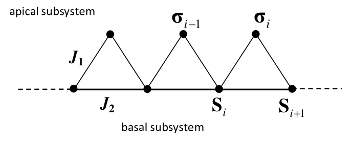
Figure 1: The delta-chain model.

The quantum $s=\frac{1}{2}$ delta-chain with antiferromagnetic (AF) exchange interactions $J_{1}$ and $J_{2}$ ($J_{1},J_{2}>0$) has been studied extensively and it exhibits a variety of peculiar properties sen ; nakamura ; blundell ; flat ; Zhit ; prl ; Derzhko2004 . At the same time the $s=\frac{1}{2}$ delta-chain with ferromagnetic $J_{1}$ and antiferromagnetic $J_{2}$ interaction (F-AF delta-chain) is very interesting as well and has unusual properties depending on the frustration parameter $\alpha=\frac{J_{2}}{\left|J_{1}\right|}$ Tonegawa ; Kaburagi ; KDNDR ; DK15 . In particular, the ground state of this model is ferromagnetic for $\alpha<\frac{1}{2}$ and it is believed Tonegawa that it is ferrimagnetic for $\alpha>\frac{1}{2}$. The critical point $\alpha=\frac{1}{2}$ is the transition point between these two ground state phases. The ground state properties of the model in this point are highly non-trivial. For example, the $s=\frac{1}{2}$ F-AF delta-chain studied in Ref. KDNDR has a class of localized magnon bound states which form a macroscopically degenerate ground state manifold hosting already half of the maximum total entropy $N\ln 2$. The $s=\frac{1}{2}$ F-AF delta-chain is a minimal model for a description of real compounds, in particular malonate-bridged copper complexes Inagaki ; Tonegawa ; ruiz ; Kaburagi as well as the new kagome fluoride Cs₂LiTi₃F₁₂, that hosts F-AF delta-chains as magnetic subsystems SUJ:PRB19 .

The $s=\frac{1}{2}$ F-AF model can be extended to the delta-chain composed of two types of spins ($\mathbf{\sigma}_{i},\mathbf{S}_{i}$) characterized by the spin quantum numbers $S_{a}$ and $S_{b}$ of the apical and basal spins, respectively. The ground state of this model is ferromagnetic (F) for $\alpha<\alpha_{c}$ and non-collinear ferrimagnetic for $\alpha>\alpha_{c}$, where $\alpha_{c}=S_{a}/2S_{b}$. The ground state of the model with any quantum numbers $S_{a}$ and $S_{b}$ in the critical point $\alpha_{c}$ consists of exact multi-magnon states as for the $s=\frac{1}{2}$ model and has similar macroscopic degeneracy KDNDR .

An additional motivation for the study of the ($S_{a},S_{b}$) F-AF delta-chain is the existence of a recently synthesized mixed $3d/4f$ cyclic coordination cluster [Fe₁₀Gd₁₀(Me-tea)₁₀(Me-teaH)₁₀(NO₃)₁₀]20MeCN (i.e. Fe₁₀Gd₁₀) S60 . This cluster consists of $10+10$ alternating gadolinium and iron ions and its spin arrangement corresponds to the delta-chain with Gd and Fe ions as the apical and basal spins correspondingly. As it was established in Ref. S60 that the exchange interaction between neighboring Fe ions is antiferromagnetic ($J_{2}\simeq 1.3K$) and the interaction between neighboring Fe and Gd is ferromagnetic ($J_{1}\simeq-2.0K$). The spin values of Fe and Gd ions are $S=\frac{5}{2}$ for Fe${}^{\text{III}}$ and $S=\frac{7}{2}$ for Gd${}^{\text{III}}$, respectively. The ground state spin of this cluster is $S=60$ which is one of the largest spins of a single molecule Sch:CP19 . This molecule is a finite-size realization of the F-AF delta-chain with $S_{a}=\frac{7}{2}$ and $S_{b}=\frac{5}{2}$. Remarkably, according to the estimate of the values of $J_{1}$ and $J_{2}$ in Ref. S60 the frustration parameter is $\alpha=0.65$, i.e. it is very close to the critical value of $\alpha_{c}=0.7$. Therefore, this molecule, although it is not directly at the critical point and located in the F phase, has properties which are strongly influenced by the nearby quantum critical point. Because the spin quantum numbers for Fe and Gd ions are rather large it seems that the classical approximation for the ($S_{a},S_{b}$) F-AF delta-chain is justified.

In our preceding work DKRS we study the classical version of the F-AF delta-chain at zero magnetic field. The ground state phase diagram of the classical model consists of the ferromagnetic at $\alpha<\alpha_{c}$ and the ferrimagnetic at $\alpha>\alpha_{c}$ phases. Remarkably, the transition between these phases occurs at the same frustration parameter $\alpha_{c}$ as in the quantum model. For $S_{a}=S_{b}$ the critical point between the ferromagnetic and ferrimagnetic phases is at $\alpha=\frac{1}{2}$. In Ref. DKRS we have obtained exact results for the partition function, the thermodynamics and spin correlation functions for different regions of the parameter $\alpha$. It was shown that the classical model provides a reasonable description of thermodynamics of Fe₁₀Gd₁₀ down to moderate temperatures. In Ref. DKRS we have studied also quantum corrections to the classical results which are essential at low temperature. It was shown that some properties of the quantum spin delta-chain are correctly described by the classical model. For example, the main features of the zero-field susceptibility $\chi$ of the quantum spin delta-chain are reproduced by the classical model. In particular, the behavior of the susceptibility in the F phase (at $\alpha<\alpha_{c}$) of the classical model coincides with the quantum model in both low and high temperature limits. The product $\chi T$ per spin diverges as $T^{-1}$ at $T\to 0$ in the infinite chain and it is proportional to $N$ for finite system and such a dependence of $\chi T$ takes place, in particular, in Fe₁₀Gd₁₀. However, the results of the paper DKRS are related to the zero field case. The experimental data for Fe₁₀Gd₁₀ presented in Ref. S60 demonstrate that there is a strong influence of a magnetic field on the low-temperature thermodynamics. That is related to the massively degenerate manifold of localized magnon states having different total magnetization. The Zeeman term will partly lift this degeneracy, this way influencing the low-energy spectrum substantially. Therefore, it is interesting to consider the thermodynamic behavior of the classical delta-chain in a magnetic field. In this paper we will study the classical delta-chain in the external magnetic field. This model is more complicated in comparison with that for $H=0$. Nevertheless, it can be solved exactly and the analytical results for the low-temperature properties are obtained explicitly. We calculate the magnetization curve $M(H)$ and the susceptibility and compare them with the results for the quantum model. For example, we can quantitatively explain the experimental result related to a maximum of $MT/H$ vs. $T$ for Fe₁₀Gd₁₀.

For simplicity and to avoid cumbersome formulas we will consider the spin-$s$ delta-chain, i.e. the model with $S_{a}=S_{b}=s$. (The extension of results for the case $S_{a}\neq S_{b}$ can be obtained straightforwardly). In accordance with the adopted simplification we will further consider the F-AF delta-chain with $s=3$ as a model for the Fe₁₀Gd₁₀ molecule.

The paper is organized as follows. In Sec. IIA we describe the ground state of the classical model (2) in different regions of the frustration parameter $\alpha$ including the critical value $\alpha=\frac{1}{2}$. The partition function and the magnetization are calculated in Sec. IIB. In Sec. IIC explicit analytical results in the low-temperature limit are presented for different regions of the parameter $\alpha$ and the scaling law for $\alpha\leq\frac{1}{2}$ is established. In Sec. III the quantum effects at low temperatures will be studied by a combination of full exact diagonalization (ED) using J. Schulenburg’s spinpack code spinpack and the finite temperature Lanczos (FTL) technique FTL1 ; FTL2 . We compare the magnetization of the classical and the quantum models and estimate finite-size effects.

II Classical spin $\Delta$-chain in a magnetic field

To obtain the classical version of Hamiltonian (1) we set $\sigma_{i}=s\vec{n}_{i}$ and $S_{i}=s\vec{n}_{i}$, where $\vec{n}_{i}$ is the unit vector at the $i$-th site. Taking the limit of infinite $s$ we arrive at the Hamiltonian of the classical delta-chain

$$\mathcal{H}=-\sum_{i=1}^{N}\vec{n}_{i}\cdot\vec{n}_{i+1}+\alpha\sum_{i=1}^{N/2}\vec{n}_{2i-1}\cdot\vec{n}_{2i+1}-h\sum_{i=1}^{N}n_{i}^{z},$$ (2)

where $N$ is the number of spins. In Eq. (2) we take the apical-basal interaction as $-1$ and the basal-basal interaction as $\alpha$.

In this Section we use the normalized magnetic field and temperature

$$h = H/s$$ (3)

$$t = T/s^{2}$$ (4)

and the corresponding inverse temperature $\beta=1/t$ to present the thermodynamic properties of model (2).

II.1 Ground state

We start our study of model (2) from the determination of the ground state. For this aim it is useful to represent Hamiltonian (2) as a sum over triangle Hamiltonians

$$\mathcal{H}=\sum_{i=1}^{N/2}\mathcal{H}_{\Delta}(i)$$ (5)

where the Hamiltonian of $i$-th triangle has the form

$$\mathcal{H}_{\Delta}(i)=-\vec{n}_{2i-1}\cdot\vec{n}_{2i}-\vec{n}_{2i}\cdot\vec{n}_{2i+1}+\alpha\vec{n}_{2i-1}\cdot\vec{n}_{2i+1}-\vec{h}\cdot(\frac{1}{2}\vec{n}_{2i-1}+\vec{n}_{2i}+\frac{1}{2}\vec{n}_{2i+1}).$$ (6)

To determine the ground state of model (5) we need to find the spin configuration on each triangle which minimizes the classical energy. It turns out that the lowest spin configuration on a triangle is different in the regions $\alpha\leq\frac{1}{2}$ and $\alpha>\frac{1}{2}$. For $\alpha\leq\frac{1}{2}$ the ground state is the trivial ferromagnetic one with all spins on each triangle pointing in the same direction. The global spin configuration of the whole system in this case is obviously ferromagnetic as well.

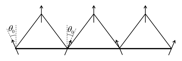
Figure 2: The ferrimagnetic ground state of classical delta-chain.

For $\alpha>\frac{1}{2}$ the lowest classical energy on each triangle is given by a non-collinear ferrimagnetic configuration, where all spins of triangle $\vec{n}_{1},\vec{n}_{2},\vec{n}_{3}$ lie in the same plane and spin $\vec{n}_{2}$ assumes an equal angle $\theta_{0}$ with spins $\vec{n}_{1}$ and $\vec{n}_{3}$. The global ground state without magnetic field of the whole system for $\alpha>\frac{1}{2}$ is macroscopically degenerate Chandra . The magnetic field lifts this degeneracy and stabilizes the ferrimagnetic configuration where all apical spins are directed along the magnetic field and the basal spins are inclined by an equal angle $\theta_{0}$ to the right and to the left of the field direction as shown in Fig. 2. Therefore,

$$\vec{h}\cdot\vec{n}_{2} = h$$ (7)

$$\vec{n}_{1}\cdot\vec{n}_{2} = \vec{n}_{2}\cdot\vec{n}_{3}=\cos\theta_{0}$$ (8)

$$\vec{n}_{1}\cdot\vec{n}_{3} = \cos\left(2\theta_{0}\right)$$ (9)

$$\cos\theta_{0} = \frac{2+h}{4\alpha}.$$ (10)

The magnetization of the ground state in the ferrimagnetic region is

$$M_{\mathrm{gs}}=\frac{2\alpha+1}{4\alpha}+\frac{h}{8\alpha}$$ (11)

for $h<h_{\mathrm{sat}}$, where the saturated field in the ground state is defined by condition $\theta_{0}=0$:

$$h_{\mathrm{sat}}=4\alpha-2.$$ (12)

II.2 Partition function

The partition function $Z$ of model (2) is

$$Z=(\prod_{i=1}^{N}\int d\vec{n}_{i})\exp\left(-\beta\mathcal{H}\right).$$ (13)

In our previous paper DKRS we used local coordinate systems associated with the $i$-th spin, which substantially simplified calculations. For the system in a magnetic field this trick does not work. Therefore, we follow a common transfer-matrix method which reduces the calculation of the partition function in 1D systems to an integral equation Blume ; Harada . In our case this integral equation is written for one triangle and has the form:

$$\int e^{-\beta\mathcal{H}_{\Delta}(1)}\psi_{i}(\vec{n}_{1})d\vec{n}_{2}d\vec{n}_{1}=\lambda_{i}\psi_{i}(\vec{n}_{3}).$$ (14)

The eigenvalues $\lambda_{i}$ define the partition function as

$$Z=\sum\lambda_{i}^{N/2}.$$ (15)

In the thermodynamic limit $N\to\infty$ only the largest eigenvalue $\lambda_{0}$ survives:

$$Z\to\lambda_{0}^{N/2}.$$ (16)

Selecting the terms containing the apical spin $\vec{n}_{2}$ in the Hamiltonian of one triangle (6)

$$\mathcal{H}_{\Delta}(1)=-\vec{n}_{2}\cdot\left(\vec{n}_{1}+\vec{n}_{3}+\vec{h}\right)+\alpha\vec{n}_{1}\cdot\vec{n}_{3}-\frac{1}{2}\vec{h}\cdot\left(\vec{n}_{1}+\vec{n}_{3}\right)$$ (17)

we can explicitly integrate the integral equation (14) over the apical spin $\vec{n}_{2}$

$$\int d\vec{n}_{2}\exp\left[\beta\vec{n}_{2}\cdot\left(\vec{n}_{1}+\vec{n}_{3}+\vec{h}\right)\right]=\frac{\sinh\left(\beta h_{a}\right)}{\beta h_{a}},$$ (18)

where $h_{a}$ is the effective magnetic field acting on the apical spin $\vec{n}_{2}$:

$$h_{a}=\sqrt{\left(\vec{n}_{1}+\vec{n}_{3}+\vec{h}\right)^{2}}.$$ (19)

Then, the integral equation (14) becomes

$$\int R(\vec{n}_{1},\vec{n}_{3})\psi_{i}(\vec{n}_{1})d\vec{n}_{1}=\lambda_{i}\psi_{i}(\vec{n}_{3})$$ (20)

with the kernel depending on the basal spins only:

$$R(\vec{n}_{1},\vec{n}_{3})=\frac{\sinh\left(\beta h_{a}\right)}{\beta h_{a}}\exp\left[-\beta\alpha\vec{n}_{1}\cdot\vec{n}_{3}+\frac{1}{2}\beta\vec{h}\cdot\left(\vec{n}_{1}+\vec{n}_{3}\right)\right].$$ (21)

Eq. (20) implies that the calculation of the thermodynamics of the delta-chain is reduced to the thermodynamics of the basal spin chain with special form of interactions, which depend on the temperature.

Now we choose the coordinate system so that the magnetic field is directed along the $Z$ axis. Then, $\vec{h}=\left(0,0,h\right)$, and unit vectors $\vec{n}$ have components $\left(\sin\theta\cos\varphi,\sin\theta\sin\varphi,\cos\theta\right)$, thus

$$\vec{n}_{1}\cdot\vec{n}_{3}=\cos\theta_{1}\cos\theta_{3}+\sin\theta_{1}\sin\theta_{3}\cos\left(\varphi_{1}-\varphi_{3}\right)$$ (22)

and the effective magnetic field (19) is

$$h_{a}=\sqrt{2+h^{2}+2\vec{n}_{1}\cdot\vec{n}_{3}+2h\left(\cos\theta_{1}+\cos\theta_{3}\right)}\ .$$ (23)

Now we notice that the kernel $R$ in Eq. (21) contains the azimuthal angles $\varphi_{1}$, $\varphi_{3}$ only as a difference $\left(\varphi_{1}-\varphi_{3}\right)$. Then we substitute for the eigenfunctions:

$$\psi_{i}\left(\vec{n}_{j}\right)=e^{im\varphi_{j}}\phi_{m,i}\left(\theta_{j}\right)$$ (24)

and in terms of $x_{j}=\cos\theta_{j}$ the integral equation (20) becomes

$$\int_{-1}^{1}K_{m}\left(x_{1},x_{3}\right)\phi_{m,i}\left(x_{1}\right)dx_{1}=\lambda_{m,i}\phi_{m,i}\left(x_{3}\right)$$ (25)

with symmetric kernel defined by an integral over $\varphi=\left(\varphi_{1}-\varphi_{3}\right)$:

$$K_{m}\left(x_{1},x_{3}\right)=\int_{0}^{2\pi}\frac{d\varphi}{4\pi}e^{im\varphi}R_{13}\left(\varphi,x_{1},x_{3}\right).$$ (26)

The largest eigenvalue is always given by $m=0$. The states with $m>0$ become relevant in calculations of transverse correlation functions Blume , which we do not consider here. Therefore, below we put $m=0$.

Thus, the thermodynamics of the delta-chain in the magnetic field (2) is reduced to the integral equation (25) over one variable, which can easily be calculated numerically. Numerical results of Eq. (25) will be discussed in the next sections.

II.3 Classical $\Delta$-chain in a magnetic field at low temperature

In general, Eq. (25) completely describes the thermodynamics of spin delta-chain in a magnetic field (2). However, in this Section we focus on the low temperature limit, where explicit analytical results for the magnetization curve are possible.

At $t\to 0$ the integration in Eq. (20) can be carried out using the saddle point method. For this aim we need to expand the kernel $R$ in Eq. (21) near its maximum. At first we notice that the effective magnetic field on the apical spin in the ground state is:

$$h_{gs} = 2+h,\qquad\alpha\leq\frac{1}{2}$$

$$h_{gs} = \frac{1}{\alpha}+\frac{1+2\alpha}{2\alpha}h,\qquad\alpha>\frac{1}{2}.$$ (27)

As follows from Eq. (27), $h_{gs}$ is of order of unity, except the case $\alpha\to\infty$ and $h=0$, which is not considered here. Therefore, in the low-temperature limit $\beta h_{a}\gg 1$ and one can neglect the second term in $\sinh\left(\beta h_{a}\right)$. Similarly, the denominator in Eq. (21) can be substituted by its ground state value, so that the kernel $R$ in the saddle point approach is approximated as

$$R\approx\frac{\exp\left(-\beta\mathcal{H}_{13}\right)}{2\beta h_{gs}},$$ (28)

where

$$\mathcal{H}_{13}=-h_{a}+\alpha\vec{n}_{1}\cdot\vec{n}_{3}-\frac{1}{2}\vec{h}\cdot\left(\vec{n}_{1}+\vec{n}_{3}\right).$$ (29)

This implies that in the low-$t$ limit the behavior of the delta chain system is described by the special form of the Hamiltonian acting on the basal chain only:

$$\mathcal{H}_{\mathrm{eff}}=-\sum\sqrt{2+2\vec{n}_{2i-1}\cdot\vec{n}_{2i+1}+2h\left(n_{2i-1}^{z}+n_{2i+1}^{z}\right)+h^{2}}+\alpha\sum\vec{n}_{2i-1}\cdot\vec{n}_{2i+1}-h\sum n_{2i-1}^{z}.$$ (30)

The integral equation (20) with the approximate expression for kernel (28) has the form:

$$\int\frac{\exp\left(-\beta\mathcal{H}_{13}\right)}{2\beta h_{gs}}\psi\left(\vec{n}_{1}\right)d\vec{n}_{1}=\lambda\psi\left(\vec{n}_{3}\right).$$ (31)

The saddle point of Eq. (31) corresponds to the ground state of the local Hamiltonian $H_{13}$. Since the ground state of $H_{13}$ is different in the regions $\alpha\leq\frac{1}{2}$ and $\alpha>\frac{1}{2}$, it is necessary to study these cases separately.

II.3.1 Ferromagnetic region and critical point $\alpha\leq\frac{1}{2}$

In the ferromagnetic region $\alpha<\frac{1}{2}$ including the vicinity of the critical point $\alpha=\frac{1}{2}$ at low $t$ nearest neighbor spins $\vec{n}_{1}$ and $\vec{n}_{3}$ are almost parallel. In the pure ferromagnetic case $\alpha=0$ the angle between the neighboring spin vectors is of the order of $t^{1/2}$ and the magnetic field scales as $h\sim t^{2}$ universality . As was pointed in Ref. DKRS , near the critical point the critical properties change so that the angle between the neighboring spin vectors is of the order of $t^{1/4}$ and as will be shown below the magnetic field scales as $h\sim t^{3/2}$ in the low-$t$ limit. Using these facts we expand the effective magnetic field acting on the apical spin as:

$$h_{a}\approx 2-\frac{1}{2}\left(1-\vec{n}_{1}\cdot\vec{n}_{3}\right)-\frac{1}{16}\left(1-\vec{n}_{1}\cdot\vec{n}_{3}\right)^{2}+\frac{1}{2}\vec{h}\cdot\left(\vec{n}_{1}+\vec{n}_{3}\right).$$ (32)

This results in the following effective local Hamiltonian (29)

$$\mathcal{H}_{13}=\left(\frac{1}{2}-\alpha\right)\left(1-\vec{n}_{1}\cdot\vec{n}_{3}\right)+\frac{1}{16}\left(1-\vec{n}_{1}\cdot\vec{n}_{3}\right)^{2}-\vec{h}\cdot\left(\vec{n}_{1}+\vec{n}_{3}\right).$$ (33)

Though the second term in Eq. (33) is of second order in the small parameter $\left(1-\vec{n}_{1}\cdot\vec{n}_{3}\right)$, it becomes relevant in the vicinity of the critical point when the factor $\left(\frac{1}{2}-\alpha\right)$ at the first order term is small.

Next, we can simplify Eq. (31) by substituting $h_{gs}=2$ from Eq. (27), and expanding the exponent with the magnetic field term ($\beta h\ll 1$):

$$\exp\left(\beta h\left(n_{1}^{z}+n_{3}^{z}\right)\right)\approx 1+\beta h\left(n_{1}^{z}+n_{3}^{z}\right)\approx 1+2\beta hn_{3}^{z}$$ (34)

which transforms Eq. (31) to the form

$$\left(1+2\beta hn_{3}^{z}\right)\int e^{-\beta\mathcal{H}\left(\vec{m}\right)}\psi\left(\vec{n}_{3}+\vec{m}\right)d\vec{m}=4\beta\lambda\psi\left(\vec{n}_{3}\right),$$ (35)

where

$$\mathcal{H}\left(\vec{m}\right)=\frac{1-2\alpha}{4}\vec{m}^{2}+\frac{1}{64}(\vec{m}^{2})^{2}$$ (36)

and

$$\vec{m}=\vec{n}_{1}-\vec{n}_{3}$$ (37)

is a small vector of length $\left|\vec{m}\right|\sim t^{1/4}$ which can be considered as a 2D vector ($m_{1}$,$m_{2}$) in the plane perpendicular to the spin vector $\vec{n}_{3}$.

Now we expand the function $\psi$ in Eq. (35) to the second order in $\vec{m}$:

$$\psi\left(\vec{n}+\vec{m}\right)=\psi\left(\vec{n}\right)+m_{i}\frac{\partial\psi\left(\vec{n}\right)}{\partial n_{i}}+\frac{1}{2}m_{i}m_{j}\frac{\partial^{2}\psi\left(\vec{n}\right)}{\partial n_{i}\partial n_{j}},$$ (38)

where derivatives are taken along two orthogonal directions in the plane perpendicular to the spin vector $\vec{n}$.

The Hamiltonian (36) is a function of $\vec{m}^{2}$. Therefore, linear terms in $m_{i}$ and terms $\sim m_{1}m_{2}$ in Eq. (38) vanish after integration over $\vec{m}$ in the integral equation (35). As a result, the integral equation (35) becomes

$$\left(1+2\beta hn^{z}\right)\psi\left(\vec{n}\right)\int e^{-\beta\mathcal{H}\left(\vec{m}\right)}d\vec{m}+\frac{1}{4}\frac{\partial^{2}\psi}{\partial n_{i}^{2}}\int e^{-\beta\mathcal{H}\left(\vec{m}\right)}\vec{m}^{2}d\vec{m}=4\beta\lambda\psi\left(\vec{n}\right),$$ (39)

where we omit the next-order terms $\sim\beta h\vec{m}^{2}$. Now we notice that

$$\frac{\partial^{2}}{\partial n_{1}^{2}}+\frac{\partial^{2}}{\partial n_{2}^{2}}=-\hat{L}^{2}$$ (40)

is nothing but the angular momentum operator. Therefore, we come to the Schrödinger equation for the quantum rotator in the gravitational field

$$\left(\frac{1}{2}\hat{L}^{2}-gn_{z}\right)\psi\left(\vec{n}\right)=\mu\psi\left(\vec{n}\right),$$ (41)

where the gravitational field

$$g=\frac{A}{B}\beta h$$ (42)

depends on the Hamiltonian $\mathcal{H}\left(\vec{m}\right)$ via the integrals $A$ and $B$:

$$A = \int e^{-\beta\mathcal{H}\left(\vec{m}\right)}d\vec{m}$$

$$B = \frac{1}{4}\int e^{-\beta\mathcal{H}\left(\vec{m}\right)}\vec{m}^{2}d\vec{m}$$ (43)

and the partition function $\lambda$ is given by the lowest eigenvalue $\mu_{0}$ by the equation

$$\lambda=\frac{A-2B\mu_{0}}{4\beta}.$$ (44)

The normalized magnetization is given by the scaling function $M(t,h)=\phi(g)$, where $\phi(g)$ is determined from the ground state energy $\mu_{0}$ of Eq. (41) by the relation universality

$$\phi(g)=-\frac{d\mu_{0}}{dg}.$$ (45)

The expansion of the function $\phi(g)$ for small and large $g$ as well as the numerical calculation of $\phi(g)$ was obtained in Ref. universality . It was shown in Ref. Marko that the function $\phi(g)$ is well described by the approximate equation

$$g=\phi(g)-\frac{1}{4}+\frac{1}{4\left(1-\phi(g)\right)^{2}}.$$ (46)

Calculating $A$ and $B$ in Eq. (43) for $\mathcal{H}\left(\vec{m}\right)$ given by Eq. (36)) we have

$$g=\frac{h}{2t^{3/2}}f(y),$$ (47)

where

$$f(y)=\left[\frac{e^{-y^{2}}}{\sqrt{\pi}[1+\text{erf}(y)]}+y\right]^{-1}$$ (48)

is the scaling function of the scaling parameter

$$y=\frac{2\alpha-1}{\sqrt{t}},.$$ (49)

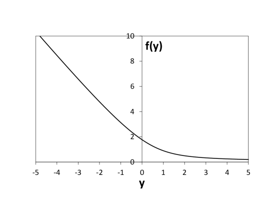
Figure 3: Scaling function $f(y)$ given by Eq. (48).

Eq. (48) represents the analytical expression for the scaling function $f(y)$ shown in Fig. 3. This function defines the magnetization curve and the zero-field susceptibility

$$\chi(t,\alpha)=\frac{1}{3t^{3/2}}f(y).$$ (50)

The behavior of the scaling function $f(y)$ defines two regions with different types of thermodynamics. The first region corresponds to the limit $y\to-\infty$, where the scaling function $f(y)$ tends to the asymptotic $f(y)=-2y$ and the gravitational field $g$ is

$$g=\frac{1-2\alpha}{t^{2}}h.$$ (51)

This region is limited by the condition $(1-2\alpha)\gg\sqrt{t}$ and extends up to the pure ferromagnetic case $\alpha=0$. Therefore, we name this region as ‘ferromagnetic’ regime. The thermodynamics in the ‘ferromagnetic’ regime is similar to that for the ferromagnetic chain. In particular, the zero-field susceptibility behaves as $\chi\sim t^{-2}$.

The second region is located near the critical point $\alpha=\frac{1}{2}$ and is restricted by the condition $|1-2\alpha|\ll\sqrt{t}$ ($|y|\ll 1$). In this ‘critical point’ region one can take the limit $f(0)=\sqrt{\pi}$ and the gravitational field becomes

$$g=\frac{\sqrt{\pi}}{2t^{3/2}}h.$$ (52)

The thermodynamics in this region is governed by the critical point. In particular, the zero-field susceptibility behaves as $\chi\sim t^{-3/2}$. The crossover between these two regimes takes place at the value $y\simeq-1$, or $t\simeq t_{0}=(1-2\alpha)^{2}$.

If we study the low-$t$ thermodynamics of the classical $\Delta$-chain for some fixed value of $\alpha$ (not far from the transition point), the above two regimes will manifest as follows. The ‘ferromagnetic’ regime taking place at very low temperatures $t\ll t_{0}$ will gradually be replaced by the ‘critical point’ regime for $t\gg t_{0}$ (but still $t\ll 1$).

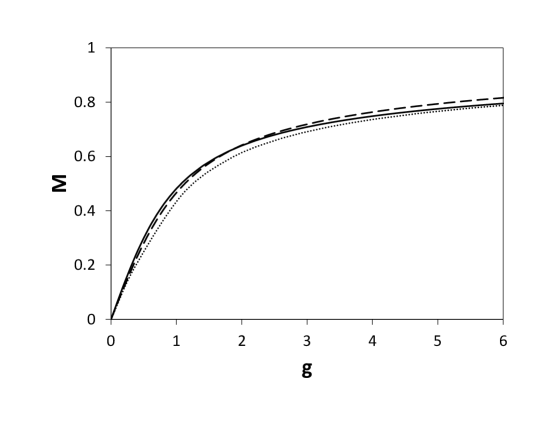
Figure 4: Magnetization curve obtained by numerical solution of the integral equation (25) and plotted as a function of the scaled magnetic gield $g$ (47) for $\alpha=0.2$ (dotted line) and $\alpha=0.5$ (dashed line) and $t=0.1$ in comparison with the scaling function $\phi(g)$ (solid line) representing the exact result in the $t\to 0$ limit.

The scaling function $\phi(g)$ describes the magnetization in $t\to 0$ limits. However, the comparison of the exact numerical solution of Eq. (25) for $\alpha=0.2$ and $\alpha=0.5$ with the scaling function given by Eq. (46) shows a good agreement of both results even for $t=0.1$ as shown in Fig. 4.

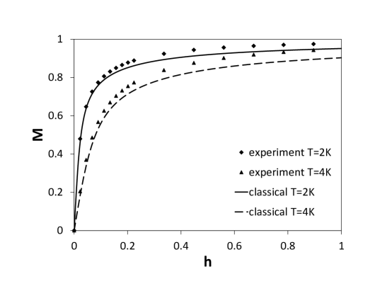
Figure 5: Magnetization curve obtained by numerical solution of the integral equation (25) for $\alpha=0.45$ in comparison with the experimental data for Fe₁₀Gd₁₀ for $T=2$ K and $T=4$ K. The real magnetic field $B$ is converted to the normalized one $h$ by equation $h=g\mu_{B}B/Jsk_{B}$ and the normalized temperature relates to real temperature by $t=T/Js(s+1)$ with $s=3$ and $J=2$ K S60 .

The comparison of the classical with the experimental magnetization curves for Fe₁₀Gd₁₀ is shown in Fig. 5. We find a reasonable agreement. The slight differences between the theoretical and the experimental curves can be attributed to quantum effects and to different apical and basal spins present in Fe₁₀Gd₁₀.

II.3.2 Ferrimagnetic region $\alpha>\frac{1}{2}$

In the ferrimagnetic region the neighboring basal spin vectors form an angle $2\theta_{0}$ in the ground state as shown in Fig. 2. In the vicinity of the transition point $(\alpha-\frac{1}{2})\ll 1$, the angle $\theta_{0}\ll 1$ (Eq. (10)), so that the ground state is close to the ferromagnetic one. In this case the approach developed in the previous subsection remains valid. This means that on the ferrimagnetic side of the transition point (and close to it) the magnetization curve is given by the same scaling function $\phi(g)$ with $g$ defined by Eq. (47). The behavior of the scaling function $f(y)$ for $y>0$ exhibits two low-$t$ regimes. The ‘critical point’ regime discussed in the previous subsection extends to the ferrimagnetic region and is restricted by the condition $(2\alpha-1)\ll\sqrt{t}$ ($y\ll 1$). In the limit $y\gg 1$ the scaling function behaves as $f(y)\sim 1/y$, which means that for very low temperature $t\ll(2\alpha-1)^{2}$ the system is in the ‘ferrimagnetic’ regime with different thermodynamic exponents. In particular, the temperature dependence of the susceptibility in this case is $\chi\sim t^{-1}$.

We stress that the above scaling approach is valid in the vicinity of the transition point only, where $\theta_{0}\ll 1$. Far from the transition point the angle $\theta_{0}$ is no longer small, and in order to describe the low temperature thermodynamics one needs to expand the local Hamiltonian near the ferrimagnetic ground state configuration described by Eq. (10). The magnetization curve in the ferrimagnetic ground state (11) and for several small values of $t$ for $\alpha=1$ is shown in Fig. 6. As can be seen the magnetization curves approach the ground state curve with decreasing $t$. According to Fig. 6 the magnetization curves have three different scales in the magnetic field which should be studied separately: $h\ll t$, $t<h<h_{\mathrm{sat}}$, and $h\geq h_{\mathrm{sat}}$.

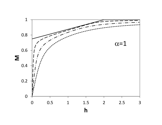
Figure 6: Magnetization curves for $\alpha=1$ and several temperatures $t=0.03$ (dashed line), $t=0.1$ (dotted-dashed line), $t=0.2$ (dotted line), obtained by numerical solution of the integral equation (25). The ground state magnetization curve (11) is shown by solid line.

For very low magnetic field, $h\ll t$, the ground state spin configurations can be described in terms of finite step random walk on the unit sphere in a weak gravitational field DKRS . The magnetization in this case increases linearly with the magnetic field and the zero field susceptibility was calculated in Ref. DKRS :

$$M = \chi h$$ (53)

$$\chi = \frac{1}{6t}\frac{2\alpha+1}{2\alpha-1}.$$ (54)

Then, for higher magnetic field $t<h<h_{\mathrm{sat}}$ the magnetization approaches its ground state value (11), and the integral equation (31) can be solved using the saddle point approximation. For this aim we introduce small deviations $\delta_{1},\delta_{3},\varepsilon$ from the ferrimagnetic ground state (10):

$$\cos\theta_{1} = \cos\theta_{0}+\delta_{1}$$

$$\cos\theta_{3} = \cos\theta_{0}+\delta_{3}$$

$$\varphi = \pi+\varepsilon.$$ (55)

The leading terms of the expansion of the local Hamiltonian in $\delta_{1},\delta_{3},\varepsilon$ is:

$$\mathcal{H}_{13}=E_{gs1}+A_{1}(\delta_{1}^{2}+\delta_{3}^{2})+2B_{1}\delta_{1}\delta_{3}+C_{1}\varepsilon^{2},$$ (56)

where

$$E_{gs1} = -\frac{(2+h)^{2}}{8\alpha}-h-\alpha$$ (57)

$$A_{1} = \frac{8\alpha^{3}(2\alpha h+h+2)-\alpha(h+2)^{2}}{[16\alpha^{2}-(h+2)^{2}](2\alpha h+h+2)}$$ (58)

$$B_{1} = A_{1}-\frac{\alpha h(2\alpha+1)(h+2)^{2}}{[16\alpha^{2}-(h+2)^{2}](2\alpha h+h+2)}$$ (59)

$$C_{1} = \frac{h(2\alpha+1)[16\alpha^{2}-(h+2)^{2}]}{32\alpha(2\alpha h+h+2)}$$ (60)

The solution of the integral equation (31) in this case is

$$\lambda=\exp\left(-\frac{E_{gs1}}{t}\right)\frac{\pi t^{2}}{h_{gs}\sqrt{A_{1}C_{1}+C_{1}\sqrt{A_{1}^{2}-B_{1}^{2}}}}.$$ (61)

The magnetization is given by the relation:

$$M=t\frac{\partial\ln\lambda}{\partial h}.$$ (62)

The magnetization curve approaches the ground state expression (11) in low-$t$ limit by the law:

$$M=M_{\mathrm{gs}}-tf_{M}\left(h,\alpha\right),$$ (63)

where the explicit form of the function $f_{M}\left(h,\alpha\right)$ is very cumbersome and we do not present it here.

Finally, when the magnetic field is higher than the saturation one, $h>h_{\mathrm{sat}}$, the ground state becomes ferromagnetic and the magnetization only slightly differs from its fully saturated value. That means that the angles $\theta_{1}$ and $\theta_{3}$ are small and the expansion of the local Hamiltonian becomes:

$$\mathcal{H}_{13} = E_{gs2}+A_{2}(\theta_{1}^{2}+\theta_{3}^{2})+2B_{2}\theta_{1}\theta_{3}\cos\varphi$$ (64)

$$E_{gs2} = -2+\alpha-2h$$ (65)

$$B_{2} = \frac{1}{2}\left(\alpha-\frac{1}{2+h}\right)$$ (66)

$$A_{2} = B_{2}+\frac{h-h_{\mathrm{sat}}}{4}.$$ (67)

In this case after some algebra the solution of the integral equation (31) yields the partition function

$$\lambda=\frac{1}{8A_{2}}\frac{t^{2}}{2+h}\exp\left(-\frac{E_{gs2}}{t}\right)\left(1+\frac{B_{2}^{2}}{4A_{2}^{2}}\right).$$ (68)

As shown in Fig. 7 for $\alpha=1$ Eqs. (53), (61), (62) and (68) perfectly describe the magnetization curve in the corresponding regions of the magnetic field.

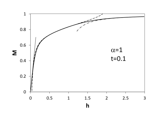
Figure 7: Magnetization curves for $\alpha=1$ and $t=0.1$ obtained by numerical solution of the integral equation (25) (solid line) and approximate equations (53), (61) and (68) in the corresponding regions (dashed lines).

III Quantum effects

In the preceding Section we represented results for the classical delta-chain in the magnetic field. Since the classical model corresponds to the limit $s\to\infty$, a natural question arises about the relation of the classical results to those of the quantum spin-$s$ model (1). In this respect it is important to mention Ref. universality where it was conjectured that the magnetization curves of the quantum and classical ferromagnetic chain coincide in the low-temperature limit and described by an universal function $\phi(g_{F})$ (Eq. (45)) of the scaling variable $g_{F}$

$$g_{F}=\frac{s^{3}H}{T^{2}}.$$ (69)

In this Section we will use non-renormalized temperature $T=ts^{2}$ and the magnetic field $H=sh$. As the ferromagnetic chain corresponds to the particular case $\alpha=0$ of our model, the problem of ‘universality’ of the classical results for $\alpha>0$ will be in the focus of our attention. Additional motivation to study the quantum effects to the classical results is that Fe₁₀Gd₁₀ is described by the quantum model with relatively high but nevertheless finite spin values. For the analysis of the magnetic properties of the quantum spin model we investigate finite chains imposing periodic boundary conditions using the numerical exact diagonalization (ED) spinpack and the finite-temperature Lanczos (FTL) technique FTL1 ; FTL2 .

III.1 Transition point

We start our analysis from the transition point $\alpha=\frac{1}{2}$. The spin-$\frac{1}{2}$ case of quantum model (1) at the transition point was studied in detail in Ref. KDNDR . It was shown that this model has many very specific properties: a flat one-magnon spectrum, localized one-magnon states and multi-magnon complexes, a macroscopic degeneracy of the ground state and a residual entropy, exponentially low-lying excitations, a multi-scale structure of the energy spectrum DK15 . It turns out that all these specific properties of the spin-$\frac{1}{2}$ model carry over to the models with higher values of spin with some inessential modifications, which we will briefly describe below.

The ground state of the quantum delta-chain with any value of $s$ at the critical point $\alpha=\frac{1}{2}$ consists of exact multi-magnon bound states exactly like the $s=\frac{1}{2}$ model and the number of the ground states, $B_{N/2}^{k}$, for fixed value $S^{z}=S_{\max}-k$ ($S_{\max}=sN$) is KDNDR

$$B_{N/2}^{k} = C_{N/2}^{k},\qquad 0\leq k\leq\frac{N}{4},\qquad 2S_{\max}-\frac{N}{4}<k\leq 2S_{\max}$$

$$B_{N/2}^{k} = C_{N/2}^{N/4},\qquad\frac{N}{4}+1\leq k\leq 2S_{\max}-\frac{N}{4}$$

where $C_{m}^{n}=\frac{m!}{n!(m-n)!}$ is the binomial coefficient.

The contribution to the partition function from only these degenerate ground states is

$$Z_{GS}=\sum_{k}B_{N/2}^{k}\exp(\frac{(S_{\max}-k)H}{T}).$$ (70)

Using a saddle-point approximation to estimate of Eq. (70) we obtain the corresponding normalized magnetization in the form

$$M_{GS}=1-\frac{1}{2s[1+\exp(H/T)]}$$ (71)

As follows from Eq. (71), the magnetization at the critical point for $H\to 0$ is

$$M_{GS}=1-\frac{1}{4s}$$ (72)

and it changes from $M_{GS}=\frac{1}{2}$ for $s=\frac{1}{2}$ to $M_{GS}=1$ for the classical limit $s\to\infty$.

Figure 8: Magnetization curves $M(H/s)$ for the quantum models with $s=\frac{1}{2}$ ($N=36$), $s=1,\frac{3}{2}$ ($N=16$), $s=2,\frac{5}{2},3$ ($N=12$) (solid lines) at the transition point $\alpha=\frac{1}{2}$ for $T/s(s+1)=0.1$. The magnetization curve of the classical model for $\alpha=\frac{1}{2}$ and $t=0.1$ is shown by the dashed line.

According to Eq. (72) the magnetization $M_{GS}$ is finite for $H\to 0$, which would clearly contradict the statement that long range order cannot exist in one-dimensional systems at $T>0$. For the correct description of $M(H,T)$ it is thus necessary to take into account the full spectrum of the model. Unfortunately, such analytical calculation is impossible, and we therefore carried out ED and FTL calculations of $M(H,T)$ for different values of $s$ and $N$. Corresponding results together with that for the classical model are shown in Fig. 8. As it can be seen from Fig. 8 the behaviors of the classical and quantum model are very different. It implies that there is no universality at the critical point. At the same time, there is one interesting point related to the behavior of the magnetization at low magnetic field. It was shown in Ref. KDNDR that the magnetization of the $s=\frac{1}{2}$ delta-chain is $M\sim H/T^{\gamma}$ with an exponent $\gamma=1.09$. On the other hand in the classical model ($s\to\infty$) $\gamma=\frac{3}{2}$ according to Eq. (50). Therefore, it can be expected that the exponent $\gamma$ is a function of $s$. To clarify this point we have calculated the zero-field susceptibility $\chi$ for different $s$ and $N$. The dependencies $\chi(T)$ are shown in Fig. 9 as log-log plot of $3\chi T/s(s+1)$ vs. $T/s(s+1)$. The solid lines denote from bottom to top: $s=\frac{1}{2}$ ($N=36$), $s=1$ ($N=16$) and $s=\frac{3}{2},2,\frac{5}{2},3$ with $N=12$. The classical curve is shown by dashed line. As it can be seen in Fig. 9 all curves tends to $1$ in the high temperature limit, which is in accord with high-$T$ behavior of the susceptibility $\chi=s(s+1)/3T$. Then, for lower temperature all curves diverge from each other and in a definite intermediate temperature region the curves have linear behavior with different slope which implies a power-law dependence

$$\chi=r(s)/T^{\gamma(s)}$$ (73)

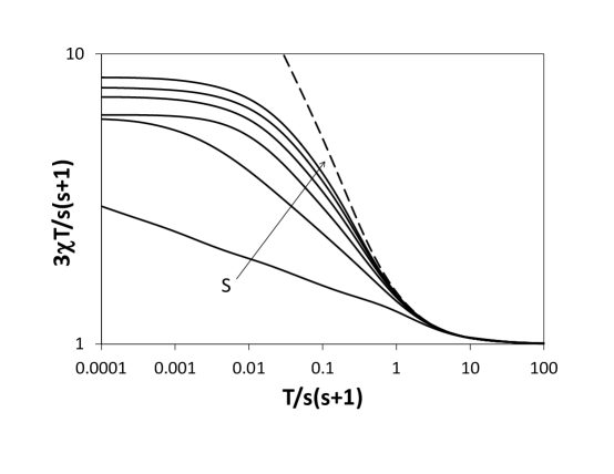
Figure 9: Dependence of $3\chi T/s(s+1)$ on the normalized temperature $T/s(s+1)$ for classical (dashed line) and quantum spin-$s$ (solid lines) delta-chain calculated at the critical point $\alpha=0.5$.

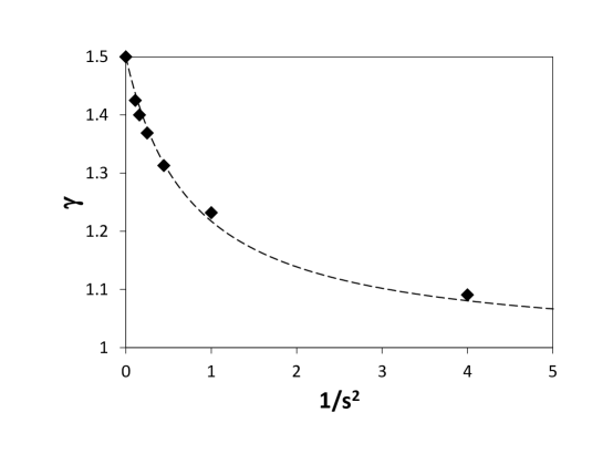
Figure 10: Dependence of the critical exponent $\gamma$ on the spin value $s$. The dashed line represents the approximate expression $\gamma=\frac{3s^{2}+2.6}{2s^{2}+2.6}$.

That means that the low-field behavior of the magnetization is $M\sim H/T^{\gamma(s)}$. The dependence of the critical exponent on spin value $\gamma(s)$ is shown in Fig. 10 and it can be seen that $\gamma\to\frac{3}{2}$ in the classical limit $s\gg 1$. As further decreasing $T/s(s+1)$ for all solid curves the sloping part in Fig. 9 is followed by a flat part related to finite-size effects. At $T\to 0$ the solid curves tend to the values determined by the contributions of the degenerate ground states. These contributions for finite delta-chains can be found by the calculations of the zero-field susceptibility per spin using Eq. (70), which results in

$$\chi=\frac{c_{N}(s)N}{T},$$ (74)

where $c_{N}(s)=\frac{1}{2}(s-\frac{1}{4})^{2}$ for $N\gg 1$. We suppose that both equations (73) and (74) for $\chi(T)$ are described by a single finite-size scaling function which has the form KDNDR

$$\chi(T)=T^{-\gamma}F(c_{N}(s)NT^{\gamma-1})$$ (75)

For small $x$ the function $F(x)$ gives (74) and in the thermodynamic limit $N\to\infty$ the scaling function tends to the value $r(s)$ in accord with Eq. (73). The crossover between these two types of the susceptibility behavior occurs at $x\simeq 1$ which defines the crossover temperature $T^{\ast}\sim N^{-1/(\gamma-1)}$. At $T<T^{\ast}$ finite-size effects are essential and $\chi$ is given by Eq. (74). The crossover temperature $T^{\ast}$ increases with $s$ and the region of finite-size behavior of $\chi$ increases.

III.2 Ferromagnetic phase

As was noted in the beginning of this Section, in the special case $\alpha=0$ the magnetization curves of both quantum and classical delta-chain models coincide in the low-temperature limit. According to the scaling hypothesis universality the normalized magnetization $M$ for the infinite chain is expressed at $T\to 0$ and $\frac{H}{T}\to 0$ (but with fixed $g_{F}$ (69)) as $M(T,h)=\phi(g_{F})$ and the function $\phi(g_{F})$ is obtained by calculating the eigenspectrum of the quantum rotator Hamiltonian (41) in the gravitational field $g_{F}$. As noted in Ref. universality the hypothesis of universality originates in the universal behavior of the spin-wave excitations above the ferromagnetic ground state in both quantum and classical models. Similarly to the case $\alpha=0$ one can expect that such universality remains in the ferromagnetic part of the ground state phase diagram ($\alpha<\frac{1}{2}$) with $g_{F}$ in Eq. (69) being replaced by

$$g_{F}=\frac{(1-2\alpha)s^{3}H}{T^{2}}.$$ (76)

in accordance with Eq. (51) for the classical model.

The universality for $\alpha<\frac{1}{2}$ is partly confirmed by the fact that the leading terms of the zero-field susceptibility at $T\to 0$ for the classical model and that obtained in a frame of the modified spin-wave theory MSWT for the quantum model coincide DKRS . Unfortunately, modified spin-wave theory is restricted to the zero magnetic field case and it can not confirm the universality of the magnetization curve.

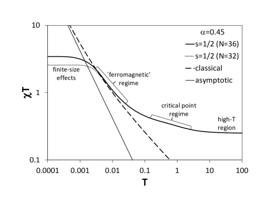
Figure 11: Susceptibility times temperature, $\chi T$, in dependence on $T$ for $\alpha=0.45$ obtained numerically by FTL for $s=1/2$ and $N=32$ (dotted line), $N=36$ (thick solid line). The classical curve is shown by the dashed line. The thin solid line describes low-$T$ asymptotic $\chi=(1-2\alpha)/24T^{2}$.

However, the extension of the hypothesis of the universality for the case $\alpha\neq 0$ and especially for $\alpha$ close to the transition point $\alpha=\frac{1}{2}$ needs some comments. As it was shown in the preceding Section the scaling parameter $g$ in the classical model has two different forms given by Eqs. (51) and (52) for $T\ll T_{0}$ and $T\gg T_{0}$, respectively, where $T_{0}=(1-2\alpha)^{2}s^{2}$ is the temperature of the crossover. For $T\ll T_{0}$ this parameter takes the form (76), while for $T\gg T_{0}$ it corresponds to that for the transition point regime, where the behavior of the classical and quantum models is very different. Therefore, one can expect that there is identical universality of the classical and quantum models in the low-temperature region $T\ll T_{0}$ only.

The quantum models also have different low-temperature regimes when $\alpha$ is close to the transition point. As an example we show in Fig. 11 the dependence of the susceptibility for the $s=\frac{1}{2}$ delta-chain and $\alpha=0.45$ with $N=32$ and $N=36$ obtained by FTL calculations, where for convenience we represent this dependence as log-log plot of $\chi T(T)$. At first we note that the curves with $N=32$ and $N=36$ perfectly coincide for $T>0.003$, which means that they correctly describe the thermodynamic limit in this region. In the high temperature limit the curves tend to a constant, which implies the correct asymptotic $\chi(T)=1/(4T)$. In the temperature range $0.1\lesssim T\lesssim 3$ the slope of the curve is very close to that obtained for $s=\frac{1}{2}$ at the transition point KDNDR : $\chi(T)\sim T^{-\gamma}$ with $\gamma=1.09$. Therefore, we refer this region to the ‘critical point’ regime.

For temperatures lower than the ‘critical point’ region the slope of the curves increases and after some crossover region the quantum curves approach the classical curve shown in Fig. 11 by a dashed line. We name the region, where the quantum curves are close to the classical one, $0.003\lesssim T\lesssim 0.02$, the ‘ferromagnetic’ one. Though the slope of the curves in this region corresponds to $\gamma\sim 1.7$ instead of a ‘ferromagnetic’ $\gamma=2$, we see that all curves converge to the ‘ferromagnetic’ low-$T$ asymptotic $\chi=(1-2\alpha)/24T^{2}$, shown by the thin solid line in Fig. 11. For $T<0.003$ the quantum curves for $N=32$ and $N=36$ diverge from each other and both from the classical curve, establishing the ‘finite-size effect’ region with non-thermodynamic behavior. Looking at Fig. 11 it is natural to assume that the quantum curve corresponding to very long chains would go further into the lower $T$ region close to the classical curve and both asymptotically approach the thin solid line, i.e., the ferromagnetic law $\chi=(1-2\alpha)/24T^{2}$. This means that for the infinite delta-chain the ferromagnetic region exists up to $T=0$. Unfortunately, for $\alpha\neq 0$ the quantum models can be studied only by numerical calculations of finite delta-chains, which due to finite-size effects restrict the low temperatures.

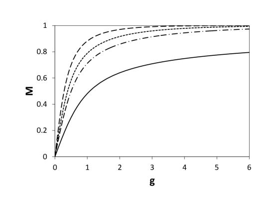
Figure 12: Magnetization curve for $\alpha=0.45$ obtained numerically by FTL for $s=1/2$, $N=36$ and three different temperatures located in the ‘ferromagnetic region’ of Fig. 11: $T=0.004$ (dashed-dotted line), $T=0.0075$ (short-dashed line), $T=0.015$ (long-dashed line). The data are plotted as a function of the scaled magnetic field $g_{F}$ (76). The exact universal magnetization curve $\phi(g_{F})$ is shown by the solid line.

The magnetization curves in the ‘ferromagnetic’ temperature region for the $s=\frac{1}{2}$ model with $N=36$ and for $\alpha=0.45$ obtained by numerical FTL calculations is shown in Fig. 12 as a function of the ‘ferromagnetically’ scaled field $g_{F}$ (76). In Fig. 12 we also show the scaling function $\phi(g)$. As it can be seen the quantum magnetization curves tend to the scaling function as the temperature decreases. However, the difference between these curves and $\phi(g)$ is rather appreciable. The point is that the function $\phi(g)$ represents the leading term in the low-temperature expansion of the magnetization. The temperatures corresponding to the magnetization of the $s=\frac{1}{2}$ model in Fig. 12 are about $T_{0}$. At such a temperature the next terms in the low-temperature expansion of the magnetization are of the same order as the leading term. This appreciable difference of the initial slope of the quantum magnetization curve and $\phi(g)$ can be also seen in Fig. 11: in the ‘ferromagnetic’ region the values $\chi(T)$ for quantum curve is approximately two times larger than that for the asymptotic line corresponding to the initial slope of $\phi(g)$. The comparison of the classical and asymptotic lines in Fig. 11 shows that the difference would become $\sim 10\%$ for $T\lesssim 0.0005$, but in order to avoid the finite-size effects at such low temperatures one needs to calculate very long chains.

In the ‘finite-size’ region the correlation length $\xi=(1-2\alpha)s^{2}/T$ is much larger than the system size (especially for $\alpha$ close to $\frac{1}{2}$) accessible in exact diagonalization (ED) ($N\sim 24$) or FTL ($N\sim 36$) calculations. In this region the finite-size effects are essential and the scaling function for the magnetization depends on two parameters $\phi(g_{F},q)$ universality with

$$q=\frac{(1-2\alpha)s^{2}}{TN}.$$ (77)

At $T\to 0$ and $q\gg 1$ the function $\phi(g,q)$ is given by the Langevin equation

$$M=\phi(g_{F},q)=\coth(x)-\frac{1}{x}$$ (78)

with

$$x=\frac{g_{F}}{q}=\frac{NsH}{T}.$$ (79)

The magnetization calculated for the quantum delta-chain at $\alpha=0.45$ with $s=\frac{1}{2}$ and $N=36$ well agrees with Eq. (78).

The numerical calculations of the magnetization of the quantum $s=\frac{1}{2}$ model for temperatures $T\gg T_{0}$ show significant difference from the classical scaling function $\phi(g)$. Therefore, we conclude that the magnetization for $0\leq\alpha<\frac{1}{2}$ is a universal function for both quantum and classical delta-chain only in the ‘ferromagnetic’ regime ($T\ll T_{0}$).

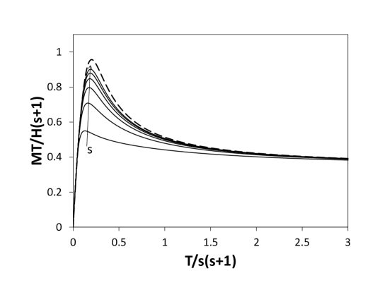
Figure 13: Comparison of quantum (solid lines) and classical (dashed line) dependencies $MT/H(s+1)$ vs. $T/s(s+1)$ calculated for $\alpha=0.45$ and $h=0.1$.

As discussed in Secs. I and II.3.1 the classical approximation for F-AF delta-chain is justified for Fe₁₀Gd₁₀, because the spin quantum numbers for Fe and Gd ions are rather large. The characteristic feature related to the susceptibility of Fe₁₀Gd₁₀ is a maximum in the temperature dependence of the quantity $MT/H$ in a fixed magnetic field. The calculation of this quantity for classical model shows good agreement with the experimental data. In particular, the maximum $(MT/H)_{max}\sim 720$ cm³K/mol is reached at $T_{max}\sim 4$ K in comparison with experimental data $(MT/H)_{max}\sim 745$ cm³K/mol is reached at $T_{max}\sim 3$ K. The temperature dependence of $MT/H$ for quantum models with different values of spin $s$ is shown in Fig. 13 together with that for the classical model. As it can be seen in Fig. 13 the dependencies $MT/H$ approach to the classical curve as $s$ increases.

III.3 Ferrimagnetic phase

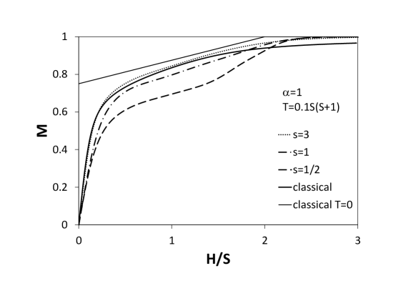
Figure 14: Comparison of the magnetization curves $M(H/s)$ for the classical (thick solid line) and quantum models with $s=1/2,N=36$ (dashed line), $s=1,N=16$ (dashed-dotted line), $s=3,N=12$ (dotted line) in the ferrimagnetic region $\alpha=1$ for $T/s(s+1)=0.1$. The ground state magnetization curve of the classical model (11) is shown by thin solid line.

The ground state of the classical model is ferrimagnetic at $\alpha>\frac{1}{2}$. As we noted before, in Ref. Tonegawa it was stated that a ferrimagnetic ground-state phase is also realized for the $s=\frac{1}{2}$ quantum delta-chain. At the same time the behavior of the magnetization curve of the classical and quantum models is very different as it is shown in Fig. 14 for $\alpha=1$. It is possible to state with certainty that there is no universality in this phase. At present it is not much known about the ground state phase of the quantum models with $s>\frac{1}{2}$ and this problem needs further study. One interesting point is the dependence of the magnetization behavior on $s$. As it is shown in Fig. 14 the magnetization curves rapidly approach to the classical one when $s$ increases. It can be expected that the magnetization of the quantum model in $s\gg 1$ limit will coincide with the classical curve.

IV Summary

In this paper we have studied the delta-chain with competing ferro- and antiferromagnetic interactions $J_{1}$ and $J_{2}$ in the external magnetic field. At $\alpha=J_{2}/|J_{1}|=1/2$, this model belongs to the class of flat-band models exhibiting a massively degenerated ground state leading to a residual entropy. Since, a magnetic field partially lifts the degeneracy, the influence of the field on the low-temperature physics is tremendous. Interestingly, there is a finite-size realization of the model, namely the magnetic molecule Fe₁₀Gd₁₀, that has $J_{1}$ and $J_{2}$ close to the flat-band point. In the present study, for the classical model exact results for the thermodynamics are obtained. It is shown that the calculation of the magnetization for $\alpha\leq\frac{1}{2}$ in the limit $T\to 0$ and $\frac{H}{T}\to 0$ reduces to the solution of the Schrödinger equation for the quantum rotator in the gravitational field $g$ which depends on the temperature. The low-temperature region of the classical model consists of two regions $T\ll T_{0}$ and $T\gg T_{0}$ ($T_{0}\sim(1-2\alpha)^{2}s^{2}$) with different type of the $g(T)$ dependence. The magnetization for $T\ll T_{0}$ is a universal function of the scaling parameter $g$ which is valid for both classical and the quantum models. In particular, the susceptibility behaves as $\chi\sim T^{-2}$. For $T\gg T_{0}$ the behavior of the magnetization and the susceptibility is the same as in the critical point $\alpha=\frac{1}{2}$ and it is different for the classical and the quantum models. In this case the susceptibility of the classical model behaves as $\chi\sim T^{-3/2}$ while $\chi\sim T^{-\gamma}$ with $\gamma=1.09$ for the quantum $s=\frac{1}{2}$ model. Generally, the value of the exponent $\gamma$ depends on $s$ and it tends to the classical value $\gamma=\frac{3}{2}$ when $s$ increases.

We compare the obtained results with the experimental data for Fe₁₀Gd₁₀, which is a finite-size realization of the considered model with $\alpha\simeq$0.45. We show that the magnetization $M(H)$ of both classical and quantum model with $s=3$ agrees well with the experimental magnetization curves measured at $T=2$ K and $T=4$ K. We also discuss the maximum in the temperature dependence of the quantity $MT/H$ at fixed magnetic field and show that it agrees very well with the experimentally observed one.

References

- (1) H. T. Diep (ed) 2013 Frustrated Spin Systems (Singapore: World Scientific).
- (2) C. Lacroix, P. Mendels and F. Mila, eds., Intoduction to frustrated magnetism. Materials, Experiments, Theory (Springer-Verlag, Berlin, 2011).
- (3) Quantum Magnetism, Lecture Notes in Physics 645, edited by U. Schollwöck, J. Richter, D. J. J. Farnell, and R. F. Bishop (Springer-Verlag, Berlin, Heidelberg, 2004).
- (4) D. Sen, B. S. Shastry, R. E. Walsteadt and R. Cava, Phys. Rev. B 53 ,6401 (1996).
- (5) T. Nakamura and K. Kubo, Phys. Rev. B 53, 6393 (1996).
- (6) S. A. Blundell and M. D. Nuner-Reguerio, Eur. Phys. J. B 31, 453 (2003).
- (7) O. Derzhko, J. Richter, M. Maksymenko, Int. J. Modern Phys. 29, 1530007 (2015).
- (8) M. E. Zhitomirsky and H. Tsunetsugu, Phys. Rev. B 70, 100403 (2004); Progr. Theor. Phys. Suppl. 160, 361 (2005).
- (9) J. Schulenburg, A. Honecker, J. Schnack, J. Richter, and H. J. Schmidt, Phys. Rev. Lett. 88, 167207 (2002).
- (10) O. Derzhko and J. Richter, Phys. Rev. B 70, 104415 (2004).
- (11) T. Tonegawa and M. Kaburagi, J. Magn. Magn. Materials, 272, 898 (2004).
- (12) M. Kaburagi, T. Tonegawa and M. Kang, J.Appl.Phys. 97, 10B306 (2005).
- (13) V. Ya. Krivnov, D. V. Dmitriev, S. Nishimoto, S.-L. Drechsler, and J. Richter, Phys. Rev. B 90, 014441 (2014).
- (14) D. V. Dmitriev and V. Ya. Krivnov, Phys. Rev. B 92, 184422 (2015); J. Phys.: Condens. Matter 28, 506002 (2016); J. Phys.: Condens. Matter 30, 385803 (2018).
- (15) Y. Inagaki, Y. Narumi, K. Kindo, H. Kikuchi, T. Kamikawa, T. Kunimoto, S. Okubo, H. Ohta, T. Saito, H. Ohta, T. Saito, M. Azuma, H. Nojiri, M. Kaburagi and T. Tonegawa, J. Phys. Soc. Jpn. 74, 2831 (2005).
- (16) C. Ruiz-Perez, M. Hernandez-Molina, P. Lorenzo-Luis, F. Lloret, J. Cano, and M. Julve, Inorg. Chem. 39 3845 (2000).
- (17) R. Shirakami, H. Ueda, H. O. Jeschke, H. Nakano, S. Kobayashi, A. Matsuo, T. Sakai, N. Katayama, H. Sawa, K. Kindo, C. Michioka, K. Yoshimura, Phys. Rev. B 100, 174401 (2019).
- (18) A. Baniodeh, N. Magnani, Y. Lan, G. Buth, C. E. Anson, J. Richter, M. Affronte, J. Schnack and A. K. Powell, npj Quantum Materials 3, 10 (2018).
- (19) J. Schnack, Contemp. Phys. 60, 127 (2019).
- (20) D. V. Dmitriev, V. Ya. Krivnov, J. Richter, and J. Schnack, Phys. Rev. B 99, 094410 (2019).
-
(21)
J. Richter, J. Schulenburg, Eur. Phys. J. B 73,
(2010) 117 (2010);
https://www-e.uni-magdeburg.de/jschulen/spinack - (22) J. Jaklic and P. Prelovsek, Phys. Rev. B 49, 5065 (1994); Adv. Phys. 49, 1 (2000).
- (23) J. Schnack and O. Wendland, Eur. Phys. J. B B 78, 535 (2010); J. Schnack, J. Schulenburg and J. Richter, Phys. Rev. B 98, 094423 (2018).
- (24) V. R. Chandra, D. Sen, N. B. Ivanov and J. Richter, Phys. Rev. B 69, 214406 (2004).
- (25) M.Blume, P.Heller, and N.A.Lurie, Phys.Rev. B11, 4483(1975).
- (26) I. Harada and H. J. Mikeska, Z. Phys. B: Condens. Matter 72, 391 (1988).
- (27) M. Takahashi, H. Nakamura, and S. Sachdev, Phys. Rev. B 54, R744 (1996).
- (28) J. F. Marko and E. D. Siggia, Macromolecules 28, 8759 (1995).
- (29) M. Takahashi, Phys. Rev. Lett. 58, 168 (1987); Phys.Rev. B 36, 3791 (1987).