Complete Spin and Valley Polarization by Total External Reflection from Potential Barriers in Bilayer Graphene and Monolayer Transition Metal Dichalcogenides

Abstract

It is shown that potential barriers in bilayer graphene (BLG) and monolayer transition metal dichalcogenides (TMDs) can split a valley unpolarized incident current into reflected and transmitted currents with opposite valley polarization. Valley asymmetric transmission inevitably occurs because of the low symmetry of the total Hamiltonian and when total external reflection occurs the transmission is 100% valley polarized in BLG and 100% spin and valley polarized in TMDs, except for exponentially small corrections. By adjusting the potential, 100% polarization can be obtained regardless of the crystallographic orientation of the barrier. A valley polarizer can be realized by arranging for a collimated beam of carriers to be incident on a barrier within the range of angles for total external reflection. The transmission coefficients of barriers with a relative rotation of $\pm\pi/3$ are related by symmetry. This allows two barriers to be used to demonstrate that the current is valley polarized. A soft-walled potential is used to model the barrier and the method used to find the transmission coefficients is explained. In the case of monolayer TMDs, a 4-band $\mathbf{k}\cdot\mathbf{p}$ Hamiltonian is used and the $\mathbf{k}\cdot\mathbf{p}$ parameters are obtained by fitting to ab-initio band structures.

I Introduction

One of the important objectives of valleytronics Vitale18 ; Amet15 ; Bussolotti18 ; Schaibley16 ; Shkolnikov02 ; Gunawan06 ; Takashina06 ; Zhu12 is to generate and detect valley polarized currents, that is currents restricted to one valley of a two-valley material. There are many proposals for electrical control of valley polarization in 2D materials Rycerz07 ; Xiao07 ; Garcia08 ; Abergel09 ; Pereira09 ; Schomerus10 ; Park12 ; Park15 ; Chen16 ; Cresti08 ; Tkachov09 ; Gunlycke11 ; Wu11 ; Koshino13 but fabrication of the necessary devices remains a challenge. This work is about an alternative approach which may be easy to realize as it only depends on components that have already been demonstrated. The idea is to arrange for carriers in one valley to be completely reflected from a potential barrier while carriers in the other valley are transmitted. This can be used to realize a valley polarizer in bilayer graphene (BLG) and a spin and valley polarizer in transition metal dichalcogenides (TMDs).

Existing proposals for valley polarizers are difficult to realize because they require structures with precise crystallographic orientation and in some cases very small size. In addition, the proposed designs typically separate the current into two streams whose direction is valley dependent. However a polarizer should produce one output stream and it is necessary to find a way of collecting the desired one. This is complicated by the strong trigonal warping of the constant energy contours in many 2D materials.

The difficulty is that the outgoing current streams typically emerge from a system of gates and because of trigonal warping the stream directions depend on the crystallographic orientation of the gates OrientationExample . However existing fabrication methods for 2D material based devices do not allow the crystallographic orientation of the 2D material to be controlled. Hence the gate orientation is unknown and in effect random. This means the desired current stream is difficult to collect because its direction is also unknown.

This difficulty does not arise in our approach because there is only one current stream on the output side of the device. The main idea is to use total external reflection to ensure that carriers in the undesired valley are reflected from the incident side of a potential barrier. This results in one current stream of practically 100% polarization in the desired valley on the transmitted side of the barrier.

Total external reflection occurs when there are propagating waves on one side of an interface but only evanescent waves occur on the other side. This situation occurs only in a certain range of incidence angles and when the energy contours are warped, this range is different in the two valleys. This results in a large angular region where the reflection is practically 100% in one of the valleys. When valley unpolarized carriers are incident within this region, the transmitted current is 100% valley polarized except for an exponentially small correction due to quantum tunneling. The valley polarization is insensitive to the barrier orientation because the barrier potential can be adjusted to optimize the region width.

These effects enable a valley polarizer to be realized by using an electron collimator to produce an incident current stream centered on the angular region required for total external reflection. The necessary collimator has been fabricated in monolayer graphene (MLG) Barnard17 and its beamwidth is similar to the angular widths of total external reflection regions in BLG and TMDs. In addition, the barrier can be realized with a structure similar to a FET. Hence the polarizer can be assembled from existing components.

In monolayer semiconducting TMDs strong spin-orbit (SO) coupling ensures that states of the same energy in opposite valleys have opposite spin. Consequently a valley polarizer made from a monolayer semiconducting TMD is also a spin polarizer.

While this work is centered on the large valley asymmetry that results from total external reflection, valley asymmetric transmission itself is inevitable because of the low symmetry of the Hamiltonian. For most barrier orientations time reversal is the only symmetry of the total Hamiltonian of the barrier and 2D material. This has the consequence that the barrier transmission coefficient is valley asymmetric but special conditions, for example total external reflection, are needed to make the asymmetry large.

The symmetry properties of the transmission coefficient are also relevant to detection of valley polarization. Although the Hamiltonian at an arbitrary barrier orientation has low symmetry, the trigonal symmetry of the constant energy contours leads to symmetry relations between the transmission coefficients for barriers of different orientation. The most important one is that the transmitted valley swaps when a barrier is rotated by $\pm\pi/3$. This means two valley polarizers may be used to demonstrate valley polarization in the same way that crossed Polaroid filters are used to demonstrate polarization of light.

In summary, the objectives of this work are first, to show that valley asymmetric transmission is a consequence of the low symmetry of the total Hamiltonian. Secondly, to show that the barrier transmission coefficient in the regime of total external reflection exhibits large valley asymmetry in both BLG and TMDs. Thirdly, to show that it should be feasible to use this effect to realize a valley polarizer and finally to show that it should be feasible to demonstrate valley polarization with a crossed pair of valley polarizers.

Existing work on valley polarization in 2D materials started with pioneering theoretical studies of valleytronics in MLG Rycerz07 ; Xiao07 . Subsequently, ways of realizing a valley polarizer were explored theoretically in a wide range of geometries in BLG and MLG, refs. Garcia08 ; Abergel09 ; Pereira09 ; Schomerus10 ; Park12 ; Park15 ; Chen16 ; Cresti08 ; Tkachov09 ; Gunlycke11 ; Wu11 ; Koshino13 for example. Other valley dependent effects are also known Low10 ; Peterfalvi12 ; Zhang13 . In addition experimental studies of valley polarization in BLG have been published recently Li20 ; Gold21 and steps have been taken towards realizing a valley polarizer Chen20 . In TMDs, optically induced valley polarization has been achieved in MoS₂ Mak14 and valley-sensitive photocurrents have been observed Zhang19 . In addition there are theoretical predictions of spin-dependent refraction at domain boundaries Habe15 and small valley polarization in crystallographically oriented potential barriers Hsieh18 . However total external reflection in graphene and TMDs has not been investigated. The present work centers on BLG and TMDs where the predicted effects should be easy to observe. Higher energies and potentials would be needed in the case of MLG Pereira09 ; Chen16 .

This paper begins with an outline of the physics (Section II) where we explain why total external reflection is valley asymmetric and give examples of valley asymmetric transmission in BLG and TMDs. Next we show that the valley asymmetric transmission is a consequence of the low symmetry of the total Hamiltonian (Section III). This requires a careful discussion because the velocity and momentum of the carriers are not parallel when trigonal warping occurs. We consider incident carriers selected by both velocity and momentum and show that valley asymmetric transmission occurs in both cases. Symmetry relations between the transmission coefficients of barriers of different orientation are also derived in this section. This is followed by an outline of the numerical methods used in this work (Section IV). Valley asymmetric transmission is detailed in sections V (BLG) and VI (TMDs). In the BLG section we first explain the device model used to obtain a realistic barrier potential, then show that potential can be adjusted to make the width of the single valley region large for all barrier orientations and finally discuss experimental feasibility. The TMD section begins with an explanation of the fitting procedure used to obtain a $\mathbf{k}\cdot\mathbf{p}$ Hamiltonian that reproduces the trigonal warping in ab-initio band structures. The remaining discussion parallels that for BLG. The feasibility of realizing a valley polarizer is examined in section VII with the conclusion that it should be possible provided that trigonal warping is strong enough and the device can be operated in the ballistic transport regime. An example of polarization detection with two crossed polarizers is given in section VIII and our results are summarized and discussed in section IX.

II Valley polarization by total external reflection

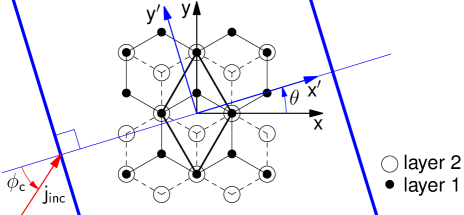
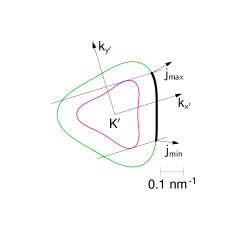
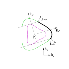
Figure 1: (Color online). Top: plan view of bilayer graphene and top gate (schematic). Bold lines (blue): gate edges; medium lines: unit cell; feint lines: bonds; open and filled circles: carbon atoms. In-plane current (j) is incident at angle $\phi_{c}$. The axis rotation angle, $\theta=17^{\circ}$. Bottom: scale drawing of energy contours and critical angles. Light outer line: contact contour (green); dark inner line: barrier contour (magenta). States on the bold part of each contact contour are transmitted. Arrows normal to the contours: critical current directions. The $KK^{\prime}$ distance is reduced so all the contours fit into one figure.

Fig. 1 illustrates how total external reflection and trigonal warping lead to valley polarized transmission through a potential barrier. The top part of the figure shows a potential barrier that is generated by a uniform bottom gate and a finite-width top gate. The top gate is rotated by an angle $\theta$ relative to the crystallographic co-ordinates, $x,y$. The external potential is expressed in co-ordinates, $x^{\prime},y^{\prime}$, fixed to the gate and is taken to be independent of $y^{\prime}$. The crystal structure is that of BLG; the geometry is similar in the case of TMDs.

The bottom part of the figure shows constant energy contours inside the barrier and the contact regions outside the barrier. The barrier contours are inside the contact contours because the potential in the barrier is higher than in the contacts so the band energy there is lower and so is the wave number, $k$. However $k_{y^{\prime}}$, the component of $\mathbf{k}$ parallel to the barrier, is a conserved quantity that is identical in the contacts and barrier.

The states in the barrier may be propagating or evanescent. Propagating states occur only in the $k_{y^{\prime}}$ range delimited by the lines that are tangential to the barrier contour and parallel to the $k_{x^{\prime}}$ axis. In this range there are two real $k_{x^{\prime}}$ values at each $k_{y^{\prime}}$ but outside the range all the $k_{x^{\prime}}$ values are complex and all the barrier states are evanescent. Then the current through the barrier is limited by tunneling and can be made exponentially small by making the barrier width sufficiently large. This is the regime of total external reflection.

Because of trigonal warping, the critical angles for total external reflection are very different in the two valleys. Propagating barrier states occur only when the contact states are in the limited range indicated by the bold lines in Fig. 1. The critical angles for total external reflection occur at the ends of this range. The current carried by a contact state with wave vector $\mathbf{k}$ is in the direction normal to the contact contour. The normals are shown in the figure and it is clear that the critical angles are very different in the two valleys.

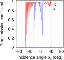
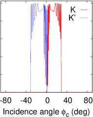
Figure 2: (Color online). Transmission coefficient for a potential barrier in BLG. The electron energy is 56 meV and the top gate width is 300 nm. Left: same-valley case, $V_{i}+U_{i}=$ 47.61 meV in layer 1, 5.586 meV in layer 2, $\theta=17^{\circ}$. Right: different-valley case, $V_{i}+U_{i}=$ 53.51 meV in layer 1, 9.124 meV in layer 2, $\theta=31^{\circ}$. See section V for details of potential.

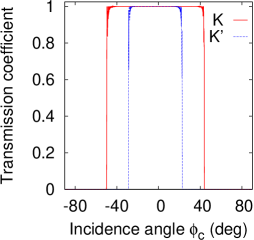
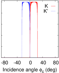
Figure 3: (Color online). Transmission coefficient for a potential barrier in MoTe₂. The hole energy is 116.9 meV and the top gate width is 300 nm. Left: same-valley case, $V=66.55$ meV, $\theta=17^{\circ}$. Right: different-valley case, $V=106.7$ meV, $\theta=31^{\circ}$. See section VI for details of potential.

The transmission coefficient as a function of current incidence angle is shown in Fig. 2 for electrons in BLG and Fig. 3 for holes in MoTe₂. In both cases the transmission coefficient approaches zero rapidly near the critical angles for total external reflection. This results in wide angular regions where the transmission coefficient is $\simeq 1$ in one valley and $\simeq 0$ in the other valley. If a collimated, valley unpolarized beam of carriers is incident on a barrier in one of these regions, the carriers in one valley are fully reflected while those in the other valley are transmitted. Hence a valley polarized current emerges on the exit side of the barrier.

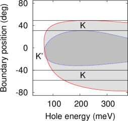
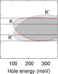
Figure 15: (Color online). Energy dependence of single valley regions in MoTe₂. The potentials and top gate width are as for Fig. 3. Solid red lines: $K$ transmission boundaries, dashed blue lines: $K^{\prime}$ boundaries. Horizontal lines indicate the beam width. Light fill: single valley transmission, dark fill: two valley transmission. Left: $\theta=17^{\circ}$ (same-valley case at $E=116.9$ meV). Right: $\theta=31^{\circ}$ (different-valley case at $E=116.9$ meV).

In general, there is one region of single valley transmission at positive angles of incidence and one at negative angles of incidence. These regions may be in the same valley or in different valleys. Figs. 2 and  3 show examples of both cases. No critical energy or potential is needed to observe these regions. They occur over a wide range of potentials and energies (Figs. 8, 13, 14 and 15) and the top gate voltage can be adjusted so they are observable at all crystallographic orientations of the barrier (Figs. 7 and 12).

III Theory

III.1 Overview

In this section we show that valley asymmetric transmission is inevitable in the presence of trigonal warping and low symmetry. The effect of trigonal warping on transmission has been investigated for some special cases Peterfalvi12 ; Park12 but the properties we need, particularly the role of points of inflection, have not been detailed and we derive them from first principles. We then show how the low symmetry of a potential barrier oriented at an arbitrary angle to the crystallographic axes inevitably leads to valley asymmetric transmission. Finally we show that the trigonal symmetry of the energy contours leads to useful symmetry relations between the transmission coefficients of barriers at different orientations.

To obtain the transmission coefficient theoretically one has to specify the direction of incidence. Experimentally, the incident particles can be selected by velocity or momentum but when the energy contours are warped, these vectors are not parallel. Hence the theoretical direction of incidence must be chosen to match the expected experimental conditions. Throughout this work the incident beam is taken to be collimated, i.e. selected by velocity, and the direction of incidence is specified by the polar angle of the incident current, $\phi_{c}$ (Fig. 1). However in this section we show that valley asymmetric transmission is inevitable regardless of whether the incident particles are selected by velocity or momentum.

This conclusion follows from straightforward but lengthy analysis. We state the Hamiltonians for BLG and TMDs in section III.2, then detail the symmetry properties of plane wave states (III.3) and currents (III.4). Next (III.5) we show how to find all the plane wave states that contribute to the incident current at angle $\phi_{c}$ (there may be more than one when there are points of inflection on the energy contour). In section III.6 we show that $k_{y^{\prime}}$ expressed as a function of $\phi_{c}$ is not the same in each valley and hence that the transmission coefficient expressed as a function of $\phi_{c}$ is valley asymmetric. Then (III.7) we prove that the transmission coefficient expressed as a function of $k_{y^{\prime}}$ is valley asymmetric because of the low symmetry of the total Hamiltonian. Finally we detail the symmetry relations between the transmission coefficients of barriers at different orientations (III.8).

III.2 Hamiltonians

The total Hamiltonians in each valley are obtained from band Hamiltonians in the literature by rotating co-ordinates anti-clockwise by an angle $\theta$ and applying a unitary transformation that reduces the $\theta$ dependence to factors of the form $\exp(\pm 3i\theta)$.

In the case of BLG and the $K$-valley, the unitary transformation is $\mathrm{diag}(e^{-i\theta},1,1,e^{i\theta})$ and the band Hamiltonian in ref. McCann13 becomes

$$H_{0K}=\left(\begin{array}[]{cccc}U_{1}&v_{0}\pi_{K}^{\dagger}&-v_{4}\pi_{K}^{\dagger}&v_{3}\pi_{K}e^{3i\theta}\\ v_{0}\pi_{K}&U_{1}+\Delta^{\prime}&t&-v_{4}\pi_{K}^{\dagger}\\ -v_{4}\pi_{K}&t&U_{2}+\Delta^{\prime}&v_{0}\pi_{K}^{\dagger}\\ v_{3}\pi_{K}^{\dagger}e^{-3i\theta}&-v_{4}\pi_{K}&v_{0}\pi_{K}&U_{2}\\ \end{array}\right),$$ (1)

where $\pi_{K}=p_{x^{\prime}}+ip_{y^{\prime}}$, $p_{x^{\prime}}$ and $p_{y^{\prime}}$ are momentum components and the parameter values are detailed in section V. The spatially uniform potentials $U_{i}$ in layer $i$ result from the bottom gate bias and the total Hamiltonian, $H_{K}=H_{0K}+V$, where $V=\mathrm{diag}(V_{1}(x^{\prime}),V_{1}(x^{\prime}),V_{2}(x^{\prime}),V_{2}(x^{\prime}))$ and $V_{i}$ is the top gate bias in layer $i$. In $K^{\prime}$, $\pi_{K}$ is replaced by $\pi_{K^{\prime}}\equiv-p_{x^{\prime}}+ip_{y^{\prime}}$ and $\theta$ by $-\theta$.

In the case of semiconducting TMDs, the band Hamiltonian for one monolayer is obtained by applying the unitary transformation $\mathrm{diag}(1,e^{i\theta},e^{-i\theta},e^{-i\theta})$ to the Hamiltonian in ref. Kormanyos13 . This gives

$$H_{0Ks_{z}}=\left(\begin{array}[]{cccc}\epsilon_{v}+\lambda s_{z}&c_{3}\pi_{K}^{\dagger}&c_{2}\pi_{K}&c_{4}\pi_{K}\\ c_{3}\pi_{K}&\epsilon_{c}&c_{5}\pi_{K}^{\dagger}e^{-3i\theta}&c_{6}\pi_{K}^{\dagger}e^{-3i\theta}\\ c_{2}\pi_{K}^{\dagger}&c_{5}\pi_{K}e^{3i\theta}&\epsilon_{v-3}&0\\ c_{4}\pi_{K}^{\dagger}&c_{6}\pi_{K}e^{3i\theta}&0&\epsilon_{c+2}-\lambda s_{z}\\ \end{array}\right),$$ (2)

where the spin index, $s_{z}=\pm 1$. The band edge energies are $\epsilon_{v}$ in the valence band, $\epsilon_{c}$ in the conduction band, $\epsilon_{v-3}$ three bands below the valence band and $\epsilon_{c+2}$ two bands above the conduction band. $c_{i}=\gamma_{i}/\hbar$ and the $\gamma_{i}$ are parameters defined in ref. Kormanyos13 . The SO splitting of the valence band is $2|\lambda|$ and the small SO splitting of the conduction band is neglected. In $K^{\prime}$, $-\lambda$ replaces $\lambda$. The parameter values are detailed in section VI.

The potential in the full TMD Hamiltonian is taken to be a scalar function, $V(x^{\prime})$ instead of the diagonal matrix that appears in the BLG Hamiltonian. This is because hole states are of interest and the effect of a perpendicular electric field on the valence bands appears to be small Rostami13 . However it is difficult to quantify this as there is no electrostatic model similar to the one in ref. McCann06 for BLG.

To analyze the symmetry of the transmission coefficients it is only necessary to consider the Hamiltonian without SO coupling. The reason is that SO coupling is negligible in BLG while in TMDs spin-valley locking occurs Xiao12 ; Liu13 . That is, the main effect of SO coupling in TMDs is to associate opposite spins with opposite valleys. For example, if there is a spin up state of energy $E$ in the $K$ valley, then there is a spin down state of energy $E$ in the $K^{\prime}$ valley. In the following, this spin reversal will be taken as understood. This allows the notation to be simplified and means the same analysis applies to BLG and TMDs.

III.3 Plane wave states

Plane wave states of energy $E$ and wave vector $\mathbf{k}$ in valley $\alpha$ satisfy

$$H_{0\alpha}\mathbf{e}_{\alpha}(\mathbf{k})\exp(i\mathbf{k}\cdot\mathbf{r}^{\prime})=E\mathbf{e}_{\alpha}(\mathbf{k})\exp(i\mathbf{k}\cdot\mathbf{r}^{\prime}),$$ (3)

where the band Hamiltonians, $H_{0\alpha}$, are defined in Eqs. (1) (BLG) and (2) (TMDs) and $\mathbf{e}_{\alpha}(\mathbf{k})$ is a 4-component polarization vector.

There are 4 distinct $\mathbf{k}$-vectors for each energy unless the energy coincides with a band extremum. Other than in this exceptional case, two of the plane wave states are propagating and two are evanescent, in the energy range considered here StateNote . However the evanescent part of the wave function vanishes at infinity. Therefore the symmetry of the transmission coefficients depends only on how the propagating wave polarization vectors transform under the symmetry operations of the full band Hamiltonian.

The full band Hamiltonian without SO coupling is the $8\times 8$ matrix

$$H_{0}=\left(\begin{array}[]{cc}\tilde{H}_{0K}&0\\ 0&\tilde{H}_{0K^{\prime}}\\ \end{array}\right),$$ (4)

where $\tilde{H}_{0\alpha}$ is the band Hamiltonian in valley $\alpha$ without SO coupling. The symmetries used in the present work are time reversal and $x^{\prime}$ inversion. The relevant invariance operators are:

Time reversal. For all $\theta$, $H_{0}$ is invariant under

$$\left(\begin{array}[]{cc}0&E_{4}\\ E_{4}&0\\ \end{array}\right)\Theta,$$ (5)

where $\Theta$ is the complex conjugation operator and $E_{4}$ is the $4\times 4$ unit matrix.

$x^{\prime}$inversion, $x^{\prime}\rightarrow-x^{\prime}$. When $\theta\equiv 0\pmod{2\pi/3}$, the $y^{\prime}$ axis is in a mirror plane of the atomic lattice and $H_{0}$ is invariant under

$$\left(\begin{array}[]{cc}0&E_{4}\\ E_{4}&0\\ \end{array}\right)I_{x^{\prime}},$$ (6)

where $I_{x^{\prime}}$ is the $x^{\prime}$ inversion operator. It follows that the polarization vectors in $K$ and $K^{\prime}$ are related as follows.

Time reversal. For all $\theta$,

$$\mathbf{e}_{K}(k_{x^{\prime}},k_{y^{\prime}})=\mathbf{e}_{K^{\prime}}^{*}(-k_{x^{\prime}},-k_{y^{\prime}}).$$ (7)

$x^{\prime}$inversion, $x^{\prime}\rightarrow-x^{\prime}$. When $\theta\equiv 0\pmod{2\pi/3}$,

$$\mathbf{e}_{K}(k_{x^{\prime}},k_{y^{\prime}})=\mathbf{e}_{K^{\prime}}(-k_{x^{\prime}},k_{y^{\prime}}).$$ (8)

III.4 Currents carried by plane wave states

The current density $\mathbf{j}_{\alpha}=(1/A)\langle\mathbf{v}_{\alpha}\rangle$ where $\langle\mathbf{v}_{\alpha}\rangle$ is the expectation value of the velocity in valley $\alpha$ and $A$ is the system area. The velocity operators are given by the matrix coefficients of the momentum terms in the band Hamiltonians. In the case of BLG

$$v_{x^{\prime}K} = \left(\begin{array}[]{cccc}0&v&-v_{4}&v_{3}e^{3i\theta}\\ v&0&0&-v_{4}\\ -v_{4}&0&0&v\\ v_{3}e^{-3i\theta}&-v_{4}&v&0\\ \end{array}\right),$$ (13)

$$v_{y^{\prime}K} = \left(\begin{array}[]{cccc}0&-iv&iv_{4}&iv_{3}e^{3i\theta}\\ iv&0&0&iv_{4}\\ -iv_{4}&0&0&-iv\\ -iv_{3}e^{-3i\theta}&-iv_{4}&iv&0\\ \end{array}\right).$$ (18)

In the case of TMDs

$$v_{x^{\prime}K} = \left(\begin{array}[]{cccc}0&c_{3}&c_{2}&c_{4}\\ c_{3}&0&c_{5}e^{-3i\theta}&c_{6}e^{-3i\theta}\\ c_{2}&c_{5}e^{3i\theta}&0&0\\ c_{4}&c_{6}e^{3i\theta}&0&0\\ \end{array}\right),$$ (23)

$$v_{y^{\prime}K} = \left(\begin{array}[]{cccc}0&-ic_{3}&ic_{2}&ic_{4}\\ c_{3}&0&-ic_{5}e^{-3i\theta}&-ic_{6}e^{-3i\theta}\\ -ic_{2}&ic_{5}e^{3i\theta}&0&0\\ -ic_{4}&ic_{6}e^{3i\theta}&0&0\\ \end{array}\right).$$ (28)

In the $K^{\prime}$ valley in both BLG and TMDs $-\theta$ replaces $\theta$ and in $v_{x^{\prime}K^{\prime}}$ the sign of the velocity parameters changes. The full velocity operator is an $8\times 8$ matrix with the same block structure as the full band Hamiltonian, Eq. (4).

The current densities in both BLG and TMDs satisfy symmetry relations that result from the polarization vector relations, Eqs. (7) and (8), and the facts that the velocity changes sign under time reversal, its $x^{\prime}$ component changes sign under $x^{\prime}$ inversion and both operations swap the blocks of the full velocity operator. The resulting symmetry relations are:

Time reversal. For all $\theta$,

$$j_{x^{\prime}K}(k_{x^{\prime}},k_{y^{\prime}}) = -j_{x^{\prime}K^{\prime}}(-k_{x^{\prime}},-k_{y^{\prime}})$$

$$j_{y^{\prime}K}(k_{x^{\prime}},k_{y^{\prime}}) = -j_{y^{\prime}K^{\prime}}(-k_{x^{\prime}},-k_{y^{\prime}}).$$ (29)

$x^{\prime}$inversion, $x^{\prime}\rightarrow-x^{\prime}$. When $\theta\equiv 0\pmod{2\pi/3}$,

$$j_{x^{\prime}K}(k_{x^{\prime}},k_{y^{\prime}}) = -j_{x^{\prime}K^{\prime}}(-k_{x^{\prime}},k_{y^{\prime}})$$

$$j_{y^{\prime}K}(k_{x^{\prime}},k_{y^{\prime}}) = j_{y^{\prime}K^{\prime}}(-k_{x^{\prime}},k_{y^{\prime}}).$$ (30)

III.5 States that carry current at angle $\phi_{c}$

To find the transmission coefficient for current incident at angle $\phi_{c}$ one has to find all the incident states that carry current at this angle. The current carried by a state with wave vector $\mathbf{k}$ flows in the direction of the group velocity $\mathbf{v}_{g}=(1/\hbar)\mbox{\boldmath$\nabla$}E(\mathbf{k})$. At constant energy, $\mathbf{v}_{g}$ only depends on the polar angle, $\phi_{k}$ of the $\mathbf{k}$-vector. The state or states that carry current at angle $\phi_{c}$, are found from the solution of

$$\phi_{v}(\phi_{k},E)=\phi_{c},$$ (31)

where $\phi_{v}$ is the polar angle of the group velocity. The group velocity may be found either from the gradient of $E(\mathbf{k})$ or from the expectation value of the velocity operator.

The number of solutions of Eq. (31) depends on whether there are points of inflection on the energy contour. In the case of TMDs there are no points of inflection and there is only one solution. However points of inflection occur in the case of BLG and three solutions occur in a small range of $\phi_{c}$.

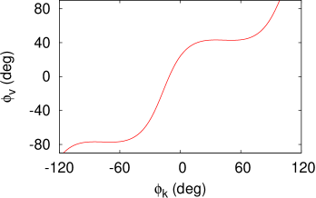
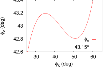
Figure 4: (Color online). Polar angle of group velocity for the $K$ valley (BLG) contact contour in Fig. 1. Upper: $-90^{\circ}\leq\phi_{v}\leq 90^{\circ}$. Lower: expanded view near $\phi_{v}=43^{\circ}$.

Fig. 4 shows $\phi_{v}(\phi_{k})$ for the case of BLG and the $K$ valley contact contour shown in Fig. 1. In most of the $\phi_{k}$ range, $\phi_{v}$ increases monotonically and $\phi_{v}(\phi_{k},E)=\phi_{c}$ has only one solution. However multiple solutions occur near $\phi_{v}=43^{\circ}$ and $-77^{\circ}$. These parts of the curve correspond to the nearly straight parts of the $K$ valley contour. $\phi_{v}(\phi_{k})$ near $\phi_{v}=43^{\circ}$ is shown on an enlarged scale in the lower part of Fig. 4. Three solutions occur between the maximum and minimum, for example at $\phi_{c}=43.15^{\circ}$. Then three distinct states carry current in the same direction and one has to sum over the currents carried by these states to find the transmission coefficient. In this work, each state is taken to contribute to the total current with equal weight.

The existence of the maximum and minimum is necessary for the multiple solutions to occur and the geometrical interpretation of this condition is that there are points of inflection on the energy contour. The vector $(-v_{gy^{\prime}},v_{gx^{\prime}})$ is tangential to the contour and by using this fact and taking the contour to be parametrized by $\phi_{k}$, the condition for a point of inflection (vanishing curvature) can be reduced to $d\phi_{v}/d\phi_{k}=0$. Hence points of inflection on the contour are necessary for multiple current carrying states to occur.

III.6 Valley Asymmetry of $T_{\alpha}(\phi_{c})$

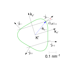
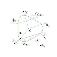
Figure 5: (Color online). Current directions (j) for all states with the same value of $|k_{y^{\prime}}|$ in the $K$ and $K^{\prime}$ valleys in BLG. The lines parallel to the $k_{x^{\prime}}$ axis indicate $|k_{y^{\prime}}|$ and the states occur at the intersections of these lines with the contact energy contours (green). Right: Current directions (black arrows) for incident (i) and reflected (r) states in $K$. The $\pm$ subscripts indicate the sign of $k_{y^{\prime}}$. Left: Current directions in the $K^{\prime}$ valley, obtained by time-reversing those in $K$. On time reversal, reflected states ($j_{x^{\prime}}<0$) in $K$ become incident states ($j_{x^{\prime}}>0$) in $K^{\prime}$. Arrows (blue) labeled $\pm k_{r-}$ and arcs (red) respectively show $\mathbf{k}$-vectors and current angles of the states discussed in section III.6. The axis rotation angle, $\theta=17^{\circ}$, and contours are as in Fig. 1.

The transmission coefficient $T_{\alpha}$ in valley $\alpha$ is the ratio of the total transmitted current to the total incident current. It can be obtained from the sum of the currents transmitted by each state that contributes to current incident at angle $\phi_{c}$. The solution of the scattering problem for each incident state gives the transmitted current as a function of $k_{y^{\prime}}$, then $T_{\alpha}(\phi_{c})$ is found by substituting $k_{y^{\prime}}(\phi_{c})$ for $k_{y^{\prime}}$. $T_{\alpha}(\phi_{c})$ is valley asymmetric because $k_{y^{\prime}}(\phi_{c})$ is not the same in each valley.

This is illustrated in Fig. 5 for a $\phi_{c}$ value for which there is only one current carrying state. There are four states with the same value of $|k_{y^{\prime}}|$ in each valley. The directions of the currents carried by these states are indicated by the arrows normal to the contours. The subscripts on the arrow labels indicate the current direction (i, incident or r, reflected) and sign of $k_{y^{\prime}}$ in the $K$ valley. The currents in $K^{\prime}$ are obtained by time-reversing those in $K$, see Eq. (29). For example, the current carried by the state incident with $k_{y^{\prime}}>0$ in $K^{\prime}$ is obtained by time reversing $\mathsf{j}_{r-}$ in $K$. The polar angles of the currents carried by states incident with $k_{y^{\prime}}>0$ are $\phi_{cKi+}$ in the $K$ valley and $\phi_{cK^{\prime}i+}$ in the $K^{\prime}$ valley. These angles are clearly different and this demonstrates $k_{y^{\prime}}(\phi_{c})$ is not the same in each valley.

The reason for this asymmetry is that the $\mathbf{k}$-vectors and currents in the $K^{\prime}$ valley are related to those in the $K$ valley by time reversal but the contours in each valley are not inversion symmetric about the valley center. Because of time reversal symmetry, the $\mathbf{k}$-vector of the incident state with $k_{y^{\prime}}>0$ in $K^{\prime}$ is $-\mathbf{k}_{r-}$ where $\mathbf{k}_{r-}$ is the $\mathbf{k}$-vector of the reflected state with $k_{y^{\prime}}<0$ in $K$. Hence the angle of incidence $\phi_{cK^{\prime}i+}$ in the $K^{\prime}$ valley is related by symmetry to the angle of reflection $\phi_{cKr-}$ in the $K$ valley. Thus $\phi_{cK^{\prime}i+}=\pi+\phi_{cKr-}$. However the angles $\phi_{cKr-}$ and $\phi_{cKi+}$ in the $K$ valley are not symmetry related because the contour is not inversion symmetric. Consequently there is in general no symmetry relation between the angles of incidence, $\phi_{cK^{\prime}i+}$ and $\phi_{cKi+}$. However the special case of $\theta\equiv 0\pmod{\pi/3}$ is an exception (section III.7).

It follows that $k_{y^{\prime}}(\phi_{c})$ is not the same function in each valley. Hence the transmitted current as a function of $\phi_{c}$ is valley asymmetric except for special incidence conditions where the curves of $T_{K}(\phi_{c})$ and $T_{K^{\prime}}(\phi_{c})$ cross. This remains true in the case of multiple current-carrying states but in this case additional asymmetry may occur because the number of current-carrying states may be different in the two valleys. Hence $T_{\alpha}(\phi_{c})$ is valley asymmetric, except for possible crossings.

III.7 Valley Asymmetry of $T_{\alpha}(k_{y^{\prime}})$

The transmission coefficient is also valley asymmetric when it is expressed as a function of $k_{y^{\prime}}$. Hence valley asymmetric transmission occurs when particles are selected by momentum as well as by velocity.

The origin of the valley asymmetry with respect to $k_{y^{\prime}}$ is that the energy contours are not mirror symmetric about the $k_{x^{\prime}}$ axis unless $\theta\equiv 0\pmod{\pi/3}$. Hence $T_{\alpha}(k_{y^{\prime}})$ in each valley is not a symmetric function of $k_{y^{\prime}}$. That is $T_{\alpha}(k_{y^{\prime}})\neq T_{\alpha}(-k_{y^{\prime}})$ unless $\theta\equiv 0\pmod{\pi/3}$. However by using time reversal symmetry it can be proved that

$$T_{K}(k_{y^{\prime}})=T_{K^{\prime}}(-k_{y^{\prime}}).$$

Therefore $T_{K}(k_{y^{\prime}})\neq T_{K^{\prime}}(k_{y^{\prime}})$, except for special incidence conditions where the curves of $T_{K}(k_{y^{\prime}})$ and $T_{K^{\prime}}(k_{y^{\prime}})$ cross.

It remains to prove that $T_{K}(k_{y^{\prime}})=T_{K^{\prime}}(-k_{y^{\prime}})$. This is done by using the $S$-matrix description of the asymptotic regime where the evanescent wave amplitudes are negligible. When $x^{\prime}$ approaches $-\infty$, the scattering states in the $K$ valley have the general form

$$\psi_{K-}=\left[i_{0}\mathbf{e}_{K}(k_{i},k_{y^{\prime}})e^{ik_{i}x^{\prime}}+r\mathbf{e}_{K}(k_{r},k_{y^{\prime}})e^{ik_{r}x^{\prime}}\right]e^{ik_{y^{\prime}}y^{\prime}}$$ (32)

and when $x^{\prime}$ approaches $+\infty$, the form is

$$\psi_{K+}=\left[t\mathbf{e}_{K}(k_{i},k_{y^{\prime}})e^{ik_{i}x^{\prime}}+x_{0}\mathbf{e}_{K}(k_{r},k_{y^{\prime}})e^{ik_{r}x^{\prime}}\right]e^{ik_{y^{\prime}}y^{\prime}}.$$ (33)

Here the $x^{\prime}$-component of the current is positive for the state with $k_{x^{\prime}}=k_{i}$ and negative for the state with $k_{x^{\prime}}=k_{r}$. $i_{0}$ is the amplitude of the incident wave, $r$ is the amplitude of the reflected wave, $t$ is the amplitude of the transmitted wave and $x_{0}$ is the amplitude of a wave incident from the right.

The asymptotic wave amplitudes are related by the $S$-matrix defined by

$$\left(\begin{array}[]{c}r\\ t\\ \end{array}\right)=\left(\begin{array}[]{cc}S_{Ka}&S_{Kb}\\ S_{Kc}&S_{Kd}\\ \end{array}\right)\left(\begin{array}[]{c}i_{0}\\ x_{0}\\ \end{array}\right).$$ (34)

The $S$-matrix is unitary provided the propagating state polarization vectors are normalized to unit current. If this normalization is not used, current conservation still constrains the form of the $S$-matrix but does not constrain it to be unitary because when the energy contours are warped, the currents carried by the incident and reflected states are not of the same magnitude. For example, the normalization $\mathbf{e}_{\alpha}(\mathbf{k})^{\dagger}\mathbf{e}_{\alpha}(\mathbf{k})=1$ is convenient for numerical calculations but with this normalization, the $S$-matrix satisfies the generalized unitarity relation $S^{\dagger}JS=\tilde{J}$ where $J=\mathrm{diag}(|j_{r}|,|j_{i}|)$ and $\tilde{J}=\mathrm{diag}(|j_{i}|,|j_{r}|)$.

The proof of the relation $T_{K}(k_{y^{\prime}})=T_{K^{\prime}}(-k_{y^{\prime}})$ is simplest when the $S$-matrices are unitary. We detail this case then state the change that is introduced by generalized unitarity. To prove the relation the $S$-matrix in the $K$ valley is related to the one in the $K^{\prime}$ valley. Application of the time reversal operator to the asymptotic states in Eqs. (32) and (33) gives

$$\psi_{K^{\prime}-} = \bigg{[}i_{0}^{*}\mathbf{e}_{K^{\prime}}(-k_{i},-k_{y^{\prime}})e^{-ik_{i}x^{\prime}}+$$ (35)

$$+ r^{*}\mathbf{e}_{K^{\prime}}(-k_{r},-k_{y^{\prime}})e^{-ik_{r}x^{\prime}}\bigg{]}e^{-ik_{y^{\prime}}y^{\prime}}$$

when $x^{\prime}$ approaches $-\infty$ and

$$\psi_{K^{\prime}+} = \bigg{[}t^{*}\mathbf{e}_{K^{\prime}}(-k_{i},-k_{y^{\prime}})e^{-ik_{i}x^{\prime}}+$$ (36)

$$+ x_{0}^{*}\mathbf{e}_{K^{\prime}}(-k_{r},-k_{y^{\prime}})e^{-ik_{r}x^{\prime}}\bigg{]}e^{-ik_{y^{\prime}}y^{\prime}}$$

when $x^{\prime}$ approaches $+\infty$. However because the sign of the current changes under time reversal, Eq. (29), the state that carries positive current in the $x^{\prime}$ direction has $k_{x^{\prime}}=-k_{r}$ and the state that carries negative current has $k_{x^{\prime}}=-k_{i}$. Consequently, the wave amplitudes in the time-reversed state are related by

$$\left(\begin{array}[]{c}i_{0}^{*}\\ x_{0}^{*}\\ \end{array}\right)=\left(\begin{array}[]{cc}S_{K^{\prime}a}&S_{K^{\prime}b}\\ S_{K^{\prime}c}&S_{K^{\prime}d}\\ \end{array}\right)\left(\begin{array}[]{c}r^{*}\\ t^{*}\\ \end{array}\right).$$ (37)

Then after using the unitarity of $S$ and complex conjugating the resulting equation, it can be seen that the $S$-matrices in the two valleys satisfy $S_{K}(k_{y^{\prime}})=S_{K^{\prime}}^{T}(-k_{y^{\prime}})$, where the sign change results from time reversal.

Next, this relation is used to prove that $T_{K}(k_{y^{\prime}})=T_{K^{\prime}}(-k_{y^{\prime}})$. The transmitted amplitude for a unit amplitude wave incident from the left is $S_{\alpha c}$ and the transmitted amplitude for a unit amplitude wave incident from the right is $S_{\alpha b}$. These amplitudes are related by $S_{Kc}(k_{y^{\prime}})=S_{K^{\prime}b}(-k_{y^{\prime}})$. In addition, $|S_{\alpha c}(k_{y^{\prime}})|=|S_{\alpha b}(k_{y^{\prime}})|$ because of unitarity. Hence $T_{K}(k_{y^{\prime}})=|S_{Kc}(k_{y^{\prime}})|^{2}=|S_{K^{\prime}b}(-k_{y^{\prime}})|^{2}=|S_{K^{\prime}c}(-k_{y^{\prime}})|^{2}=T_{K^{\prime}}(-k_{y^{\prime}})$. These relations remain valid when the $S$-matrices satisfy the generalized unitarity relation but in this case the $S$-matrices in the two valleys are related by $J_{K}S_{K}(k_{y^{\prime}})\tilde{J}_{K}^{-1}=S_{K^{\prime}}^{T}(-k_{y^{\prime}})$.

In the special case of $\theta\equiv 0\pmod{\pi/3}$, the transmission coefficient expressed as a function of $k_{y^{\prime}}$ has higher symmetry: when the potential is symmetric under $I_{x^{\prime}}$, $T_{\alpha}(k_{y^{\prime}})=T_{\alpha}(-k_{y^{\prime}})$ hence $T_{K}(k_{y^{\prime}})=T_{K^{\prime}}(k_{y^{\prime}})$. This can be proved by applying $I_{x^{\prime}}$ to the asymptotic states in Eqs. (32) and (33) and then using the definition of the $S$-matrix.

When multiple current-carrying states occur, the transmission is valley asymmetric for each state, except when $\theta\equiv 0\pmod{\pi/3}$. Hence $T_{\alpha}(k_{y^{\prime}})$ is valley asymmetric except for possible crossings and except when $\theta\equiv 0\pmod{\pi/3}$.

III.8 Transmission Coefficient Relations

The transmission coefficients at different values of $\theta$ are related by symmetry and we have found two particularly useful symmetry relations. The first is

$$T_{K}(\phi_{c},\theta)=\hat{T}_{K^{\prime}}(\phi_{c},\theta\pm\pi/3),$$ (38)

where $\hat{T}$ is the transmission coefficient for a barrier with the spatially inverted potential, $V(-x^{\prime})$. The second symmetry relation is

$$T_{K}(\phi_{c},\theta)=T_{K^{\prime}}(-\phi_{c},\pm\pi/3-\theta).$$ (39)

In both relations it is understood that the spins are opposite in the case of TMDs.

The symmetry relations occur because there are operators that transform the band Hamiltonian $H_{0K}(\theta)$ into $H_{0K^{\prime}}(\theta\pm\pi/3)$ and $H_{0K^{\prime}}(\pi/3-\theta)$. To show this $T_{\alpha}$ is first taken to be a function of $k_{y^{\prime}}$.

Then the relation equivalent to Eq. (38) is

$$T_{K}(k_{y^{\prime}},\theta)=\hat{T}_{K^{\prime}}(k_{y^{\prime}},\theta\pm\pi/3).$$ (40)

This is a consequence of the way the band Hamiltonians transform under the product of spatial inversion, $I_{x^{\prime}y^{\prime}}$, and complex conjugation, $\Theta$. The momentum transforms as $I_{x^{\prime}y^{\prime}}\Theta\pi_{K}\Theta I_{x^{\prime}y^{\prime}}=-\pi_{K^{\prime}}$ and the Hamiltonians satisfy

$$DI_{x^{\prime}y^{\prime}}\Theta H_{0K}(\theta)\Theta I_{x^{\prime}y^{\prime}}D=H_{0K^{\prime}}(\theta\pm\pi/3),$$ (41)

where $D=\mathrm{diag}(1,-1,-1,1)$ in the case of BLG and $D=\mathrm{diag}(-1,1,1,1)$ in the case of TMDs. Hence if $\psi$ is an eigenstate of $H_{0K}(\theta)+V(x^{\prime})$, then $DI_{xy}\Theta\psi$ is an eigenstate of $H_{0K^{\prime}}(\theta\pm\pi/3)+V(-x^{\prime})$ and the symmetry relation, Eq. (40), is proved. The relation holds for any $y^{\prime}$-independent potential.

The second symmetry relation, Eq. (39), is equivalent to

$$T_{K}(k_{y^{\prime}},\theta)=T_{K^{\prime}}(-k_{y^{\prime}},\pm\pi/3-\theta).$$ (42)

This is a consequence of the transformation of the Hamiltonians under inversion of the $y^{\prime}$ co-ordinate, $I_{y}^{\prime}$. In this case $I_{y^{\prime}}\pi_{K}I_{y^{\prime}}=-\pi_{K^{\prime}}$ and the Hamiltonians satisfy

$$DI_{y^{\prime}}H_{0K}(\theta)I_{y^{\prime}}D=H_{0K^{\prime}}(\pm\pi/3-\theta),$$ (43)

which leads to Eqs. (42).

The symmetry relations expressed as a function of $\phi_{c}$, Eqs. (38) and (39), follow from relations between the current components. By transforming the polarization vectors with $DI_{x^{\prime}y^{\prime}}\Theta$, it can be shown that $\mathbf{j}_{K}(\mathbf{k},\theta)=\mathbf{j}_{K^{\prime}}(\mathbf{k},\theta\pm\pi/3)$. Hence $\phi_{cK}(\theta)=\phi_{cK^{\prime}}(\theta\pm\pi/3)$ and this together with Eq. (40) leads to Eq. (38). Similarly ${j}_{x^{\prime}K}(k_{x^{\prime}},k_{y^{\prime}},\theta)=j_{x^{\prime}K^{\prime}}(k_{x^{\prime}},-k_{y^{\prime}},\pm\pi/3-\theta)$ and ${j}_{y^{\prime}K}(k_{x^{\prime}},k_{y^{\prime}},\theta)=-j_{y^{\prime}K^{\prime}}(k_{x^{\prime}},-k_{y^{\prime}},\pm\pi/3-\theta)$. Hence $\phi_{cK}(\theta)=-\phi_{cK^{\prime}}(\pm\pi/3-\theta)$ and this together with Eq. (42) leads to Eq. (39). These symmetry relations are valid for all $\phi_{c}$ hence remain valid when there is more than one current carrying state.

IV Numerical Methods

IV.1 Transmission Coefficients

The transmission coefficients are found numerically because we need to consider soft-walled barriers (Section V.2) for which the transmission coefficient cannot be found analytically. The numerical procedure is based on an S-matrix method Maksym97 that is used in surface science and is numerically stable when evanescent waves are present. In brief, the system is divided into short segments and the segment S-matrices are combined to find the system S-matrix and transmission coefficient. The segments must be short enough to allow the segment S-matrix to be computed from the segment transfer matrix to the required accuracy. The only difference between the procedure used in surface science and the present one is the method used to compute the transfer matrices.

The transfer matrices are obtained from the numerical solution of

$$(H_{0\alpha}+V_{c}+\Delta V)\psi_{\alpha}=E\psi_{\alpha},$$ (44)

where $H_{0\alpha}$ is the band Hamiltonian in valley $\alpha$ and $V_{c}$ is the position independent potential in the contacts. $\Delta V(x^{\prime})=V(x^{\prime})-V_{c}$ where $V(x^{\prime})$ is the total potential. The 4-component wave function is expressed in the form

$$\psi_{\alpha}=\exp(ik_{y^{\prime}}y^{\prime})\sum_{j=1}^{4}Q_{j}(x^{\prime})\mathbf{e}_{\alpha}(k_{j},k_{y^{\prime}})\exp(ik_{j}x^{\prime}).$$ (45)

The transfer matrix, $M$, for a segment of length $l$ with right boundary at position, $x^{\prime}$ is defined by

$$D(x^{\prime}-l)\mathbf{Q}(x^{\prime}-l)=M(x^{\prime}-l,x^{\prime})D(x^{\prime})\mathbf{Q}(x^{\prime}),$$ (46)

where $\mathbf{Q}(x^{\prime})$ is a vector whose elements are $Q_{j}(x^{\prime})$ and $D(x^{\prime})$ is a diagonal matrix whose diagonal elements are $\exp(ik_{j}x^{\prime})$.

$M$ is found by solving a differential equation for $\mathbf{Q}(x^{\prime})$. By substituting the form of $\psi_{\alpha}$ given by Eq. (45) into Eq. (44) and using the fact that the polarization vectors are orthogonal with respect to $v_{x}$ Maksym18 it can be shown that

$$\frac{d}{dx^{\prime}}\mathbf{Q}=\frac{-i}{\hbar c}D^{-1}P_{L}\Delta VP_{R}D\mathbf{Q},$$ (47)

where $P_{R}$ is a matrix whose columns are $\mathbf{e}_{\alpha}(k_{j},k_{y^{\prime}})$, $P_{L}$ is a matrix whose rows are $A_{j}\mathbf{e}^{\dagger}_{\alpha}(k_{j}^{*},k_{y^{\prime}})$ and $c=v_{0}$ in the case of BLG and $c=c_{3}$ in the case of TMDs. The constants $A_{j}$ are chosen so that $A_{j}\mathbf{e}^{\dagger}_{\alpha}(k_{j}^{*},k_{y^{\prime}})v_{x}\mathbf{e}_{\alpha}(k_{j},k_{y^{\prime}})=c$.

The calculation of the segment S-matrix requires half of the transfer matrix and half of its inverse Maksym97 . Each column of both matrices is found by solving Eq. (47) numerically with a fourth order Runge-Kutta method and appropriate initial conditions. The relative error in the transmission coefficients is $<10^{-6}$. The procedure defined by Eq. (47) is not the only way of finding the transfer matrix but we have not investigated the alternatives. The procedure can be generalized to deal with the case of $y^{\prime}$-dependent potentials.

IV.2 Propagating Region Boundaries

To find the range of current angles where single valley transmission occurs one has to find the range of current angles, $\phi_{c}$, on the propagating part of the energy contour in each valley, see bold lines and vectors normal to the contours in Fig. 1. The extrema of the current angle occur either at the end points of the propagating range or at points of inflection in the propagating range. Hence to find the range of current angles in the propagating part of the contour, one has to compute the current angles at the end points of the propagating part and at the points of inflection, then choose the angles that give the largest range. This method was used to find the propagating part of each contact contour in Fig. 1 and the regions of single valley transmission detailed in sections V and VI. In the case of Fig. 1, points of inflection occur within the propagating part but the extrema of the current angle occur at the end points.

V Single valley transmission in BLG

V.1 Overview

In this section we explain the device model used to find the barrier potential in BLG, detail the valley asymmetric transmission and show that the barrier potential can be adjusted so that large valley asymmetry occurs for all barrier orientations. We also give an extended discussion of the feasibility of observing the predicted valley asymmetry.

The device model and potential are detailed in section V.2. We then explain the valley asymmetric transmission section (V.3) and show that large valley asymmetry can be obtained for all barrier orientations by adjusting the potential (V.4). Next we show that the valley asymmetry persists over a range of Hamiltonian parameters (V.5) and is insensitive to substrate interactions (V.6). The section closes with a discussion of the requirements for observing the predicted valley asymmetry (V.7).

V.2 Model device and potential

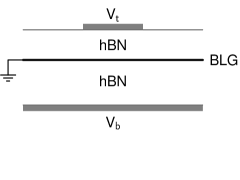
Figure 6: Cross section of device used to find model potential (schematic). The filled rectangles represent the top and bottom gates.

The barrier is taken to be generated by a device that has a narrow top gate and a wide bottom gate (Fig. 6). The bottom gate is 16 nm below the BLG and the top gate is 4 nm above it. The BLG is grounded and the space between the BLG and the gates is occupied with hBN. The electrostatic potentials in this device are estimated from a self-consistent solution of the Laplace equation based on the theory in ref. McCann06 and the numerical method in ref. Maksym19 . This allows the potential to be found for a realistic device structure but the potential is approximate because of approximations made in the theory.

The self-consistent potential is constant underneath the top gate and approaches a different constant in the contacts. Near the top gate edges it has the form of a soft step that varies monotonically between the two constant values. The self-consistent calculation of the potential is expensive but we only need potentials for a small range of device parameters. We therefore fit a model potential to the self-consistent one.

The contact potentials, $U_{1}=14$ meV, $U_{2}=-14$ meV, are obtained with a bottom gate voltage $\sim 2000$ mV. All calculations are done for these fixed values. The top gate voltage is varied over a small range to optimize the widths of the single valley regions. Within this range, the total potential is taken to vary linearly with top gate voltage, $V_{t}$,

$$U_{1}+V_{1} = V_{01}+\frac{dV_{1}}{dV_{t}}\Delta V_{t},$$

$$U_{2}+V_{2} = V_{02}+\frac{dV_{2}}{dV_{t}}\Delta V_{t},$$

where $V_{01}=37$ meV, $V_{02}=-0.78$ meV are the total potentials when $V_{t}\sim-200$ mV and $dV_{1}/dV_{t}=-0.12$, $dV_{2}/dV_{t}=-0.072$ are estimated by numerical differentiation of the self-consistent potential.

The model step function is chosen to reproduce the self-consistent potential. We have found that the self-consistent potential varies rapidly near the gate edges and slowly far from the gate edges. This variation cannot be reproduced well with a function that depends only on one length parameter, however a reasonable approximation is

$$F(x^{\prime}) = \frac{1}{2}[1+\tanh(x^{\prime}/a)],\quad x^{\prime}>x_{0},$$ (48)

$$= \frac{\alpha}{(x^{\prime}-\beta)^{2}+\gamma},\quad x^{\prime}\leq x_{0},$$

where two of the parameters are constrained by the requirements that $F$ and $dF/dx^{\prime}$ are continuous at $x^{\prime}=x_{0}$. The parameters $a,x_{0}$ and $\gamma$ are used to adjust the shape of $F$ while $\alpha$ and $\beta$ are used to enforce continuity. The continuity requirement can be satisfied with two different values of $\alpha$ and $\beta$; the values that give the best fit are chosen. The resulting parameter set is $a=3$ nm, $x_{0}=2.5$ nm, $\gamma=20$ nm², $\alpha=17.89$ nm² and $\beta=3.626$ nm. $F(x^{\prime})$ defined in Eq. (48) gives an upward step, the downward step is modeled with $F(-x^{\prime})$ so the barrier is symmetric.

V.3 Valley asymmetric transmission

	Set 1	Set 2	Set 3
$\gamma_{0}$	3160	3000	2900
$\gamma_{3}$	380	300	100
$\gamma_{4}$	140	150	120
$t$	381	400	300
$\Delta^{\prime}$	22	18	0

Table 1: Bilayer graphene Hamiltonian parameters in meV. The velocity parameters are related to the $\gamma$ parameters by $v_{i}=a\gamma_{i}\sqrt{3}/2\hbar$, where $a=0.246$ nm is the lattice constant. The parameters are taken from Table 1 in ref. McCann13 . In parameter set 3, $\Delta^{\prime}$ is not given in ref. McCann13 and is assumed to be 0.

The valley asymmetric transmission is shown in Fig. 2. The transmission coefficients are computed as described in section IV.1 and with Hamiltonian parameter set 1 in Table 1. Multiple current carrying states occur only in a narrow $\phi_{c}$ range, $\sim 0.4^{\circ}$. The sensitivity to the parameter values is discussed in section V.5.

Two types of valley asymmetry occur. When $\theta$ is not close to $\pi/6\pmod{2\pi/3}$ and not close to $\pi/2\pmod{2\pi/3}$ (Fig. 2, left) single valley transmission occurs in the same valley at both positive and negative $\phi_{c}$. But when $\theta$ is close to $\pi/6\pmod{2\pi/3}$ or close to $\pi/2\pmod{2\pi/3}$ (Fig. 2, right) the single valley transmission at positive and negative $\phi_{c}$ is in different valleys.

In both cases the transmission coefficient is large in a central region and goes to zero abruptly at two critical angles. In the central region the barrier states are propagating and transmission resonances occur. The resonances are sharp because the barrier is wide. Beyond the two critical angles, the barrier states are evanescent. Then tunneling occurs in the barrier and when the barrier width is large, the transmission coefficient is exponentially small. With the 300 nm gate width assumed in this work, the transmission coefficient is typically between $10^{-4}$ - $10^{-3}$ at about 0.1^∘ into the tunneling regime and several orders of magnitude smaller a few degrees into it. Then the transmission coefficient is practically zero and valley asymmetric total external reflection occurs as explained in section II. In addition, Fig. 1 shows that the range of incident current angles is larger in $K$ than in $K^{\prime}$. This explains why the width of $T_{K}$ in Fig. 2 (left) is larger than the width of $T_{K^{\prime}}$.

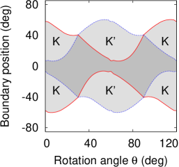
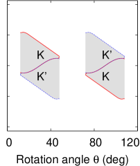
Figure 7: (Color online). Optimized single valley regions for 56 meV electrons in BLG. Solid red lines: $K$ transmission boundaries, dashed blue lines: $K^{\prime}$ boundaries. Light fill: single valley transmission, dark fill: two valley transmission. Left: same valley at $\pm$ incidence. Right: different valleys at $\pm$ incidence; in this case sharp cut-offs occur and, for clarity, some tiny regions are not shown; see section V.4 and Fig. 9.

V.4 Optimized single valley transmission

Fig. 2 shows that single valley transmission occurs in two regions that are bounded by critical angles for total external reflection. It is desirable to maximize the angular width of the single valley regions. We do this by varying the top gate voltage: the region boundaries are computed as described in section IV.2 and the gate voltage is adjusted to maximize the region widths.

Fig. 7 shows this leads to large angular widths. By choosing the case when the valleys are the same on both sides of $0^{\circ}$ (left) or different (right), single valley regions of width $\sim 17.3-53.0^{\circ}$ can be obtained for all $\theta$. The $\theta$ dependence of the single valley regions is quite different in the same-valley and different-valley cases. The explanation is as follows.

In the same-valley case, single valley regions of finite width are found for all $\theta$ except $\theta=\pi/6$ and $\theta=\pi/2$. When $\theta=\pi/6$, it follows from Eq. (39) that $T_{K}(\phi_{c},\pi/6)=T_{K^{\prime}}(-\phi_{c},\pi/6)$. Hence if single valley transmission occurs in one valley $\alpha$ for $\phi_{c}>0$, it must occur in the other valley when $\phi_{c}<0$. Therefore the same-valley case cannot occur at $\theta=\pi/6$ for any value of the potential. In the case of $\theta=\pi/2$, the fact that the barrier is symmetric gives $\hat{T}_{\alpha}=T_{\alpha}$ and it then follows from Eq. (38) that $T_{K}(\phi_{c},\pi/6)=T_{K^{\prime}}(\phi_{c},\pi/2)$ and $T_{K^{\prime}}(-\phi_{c},\pi/6)=T_{K}(-\phi_{c},\pi/2)$. These relations together with the relation $T_{K}(\phi_{c},\pi/6)=T_{K^{\prime}}(-\phi_{c},\pi/6)$ lead to $T_{K}(\phi_{c},\pi/2)=T_{K^{\prime}}(-\phi_{c},\pi/2)$. Again, the same-valley case cannot occur for any value of the potential. These arguments explain why the single valley regions widths in the same-valley case shrink to zero at $\theta=\pi/6$ and $\theta=\pi/2$.

In the different-valley case, single valley regions of large width occur near $\theta=\pi/6$ and $\theta=\pi/2$ but sharp cut-offs occur as $\theta$ departs from these values. Beyond the cut-offs it is difficult or even impossible to find potentials that lead to different-valley behavior. This is a consequence of the $\theta$ dependence of the propagating part of each energy contour. When $\theta$ changes, one end point of a propagating part may go around a corner of a contour. When this happens, $\phi_{c}$ changes rapidly with $\theta$ and the propagating range broadens rapidly. If the propagating range in the other valley remains narrow, a crossover from different-valley to same-valley behavior may occur.

For example, consider the cut-off near $\theta=12^{\circ}$ in Fig. 7. If $\theta$ decreases from $\sim 30^{\circ}$, the end point of the propagating range in the $K$ valley moves around the right hand corner of the contour. Then a crossover to same-valley behavior occurs but the different-valley behavior can be restored by raising the barrier height. This shrinks the barrier contour (Fig. 1) hence shrinks the propagating part of the contact contours in both valleys and restores the different-valley behavior. However the barrier height cannot be raised above $E$ as the transmission becomes exponentially small. This condition corresponds to the cut-off near $\theta=12^{\circ}$ and all the other cut-offs.

Beyond the cut-offs tiny regions of different-valley behavior can be found by changing the potential drastically. These regions correspond to $\theta$ and $\phi_{c}$ ranges of only a few degrees which is too small to be of practical use. For this reason and for clarity they are not shown in Fig. 7 but are detailed in section V.5.

The rapid variation of $\phi_{c}$ when the end point of a propagating part goes around a corner of an energy contour also affects the same-valley behavior. This is why small peaks and dips occur in the same-valley boundary lines near $\theta=0$, $60$ and $120^{\circ}$.

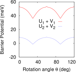
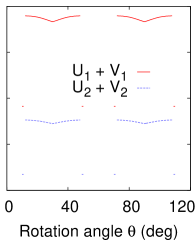
Figure 8: (Color online). Optimal barrier potentials in BLG. The corresponding single valley regions are shown in Fig. 7. Left: same-valley case. Right: different-valley case.

Fig. 8 shows the optimal barrier potentials used to compute the single valley region boundaries shown in Fig. 7. The range of potentials needed for two single valley regions in the same valley does not overlap with the range needed for two single valley regions in different valleys. In addition, if the region widths are calculated with a $\theta$-independent potential, equal to the mid-range optimal potential, they shrink by $\sim 10$-$20$%. These observations confirm it is necessary to adjust the top gate voltage to get single valley regions of large width for all $\theta$.

The required bias is modest and outside the range needed for a Lifshitz transition. A Lifshitz transition occurs in BLG when the interlayer bias is either very low McCann13 or very high Boswami13 . This does not affect the valley asymmetry but causes the energy contours to become disconnected and may be inconvenient because the transmitted current may be reduced. However the bias values in Fig. 8 are not in the range where disconnected contours occur.

V.5 Sensitivity to Hamiltonian Parameters

A wide range of Hamiltonian parameters appears in the literature so it is important to check the sensitivity of the single valley region widths to the parameter values (Table 1). This is done by repeating the calculations with parameter sets 2 and 3.

Fig. 9 shows region boundaries computed with parameter sets 1 and 2. The boundaries computed with parameter set 1 are identical to those in Fig. 7 and the tiny regions of different-valley behavior, which are omitted from Fig. 7 also shown. When parameter set 2 is used the range of single valley region widths becomes $\sim 17.4-47.0^{\circ}$ which is similar to the range found with parameter set 1. If parameter set 3 is used, the single valley range is smaller, $\sim 7.5-18.3^{\circ}$ (Fig. 10). However the range width depends on energy and when the energy is decreased to 19 meV, the range width becomes $\sim 9.6-29.0^{\circ}$.

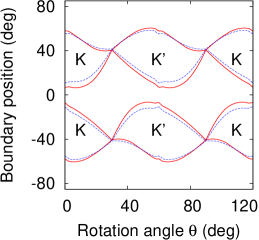
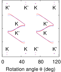
Figure 9: (Color online). Optimized single valley regions in BLG. Solid red lines: $K$ and $K^{\prime}$ region boundaries computed with parameter set 1 as in Fig. 7; dashed blue lines: $K$ and $K^{\prime}$ boundaries computed with parameter set 2. Left: same-valley case. Right: different-valley case. See Table 1 for parameter values.

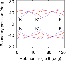
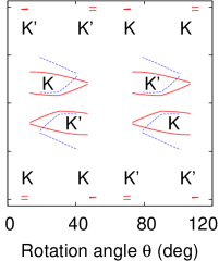
Figure 10: (Color online). Optimized single valley regions in BLG. Solid red lines: region boundaries computed with parameter set 3 and $E$ = 56 meV; dashed blue lines: boundaries computed with $E$ = 19 meV. Left: same-valley case. Right: different-valley case. See Table 1 for parameter values.

V.6 Sensitivity to Substrate

There are reports that a small band gap occurs in MLG on an hBN substrate mlggap . If a similar gap occurred in BLG on hBN it could affect the single valley regions, however there is experimental and theoretical evidence that this effect is either small or experimentally controllable. In particular, the authors of ref. Varlet14 were able to explain their data on Fabry-Perot resonances in a BLG potential barrier without considering interactions with the substrate. This is consistent with the ab-initio density functional calculations in ref. Ramasubramaniam11 . The authors of this reference computed the band structure of 3 different BLG-hBN heterostructures and found that a substrate-induced gap occurs only in one case where the heterostructure is asymmetric. The gap in this case is about 40 meV.

If a gap of this magnitude occurs, its effect can be compensated for by adjusting the gate voltage. To show this, the optimization calculations leading to Fig. 7 are repeated with substrate interactions included. In ref. Ramasubramaniam11 the 40 meV gap results from a $\sim+13$ meV shift of the conduction band edge and a $\sim-27$ meV shift of the valence band edge. The gap and shifts are modeled by adding the mass terms $\mathrm{diag}(13,-13,27,-27)$ to the Hamiltonian. These terms are similar to the mass terms given by other authors McCann13 ; Predin16 but are made asymmetric to model the asymmetric shifts of the band edges in ref. Ramasubramaniam11 .

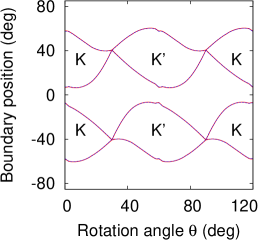
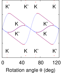
Figure 11: (Color online). Effect of gap on optimized single valley regions in BLG. Solid red lines: $K$ and $K^{\prime}$ region boundaries computed with parameter set 1 as in Fig. 7; dashed blue lines: $K$ and $K^{\prime}$ boundaries computed with gap included. Left: same-valley case. Right: different-valley case.

The optimized region boundaries with the gap included (Fig. 11) are almost identical to those computed without including the gap. The only differences are that the tiny regions of single valley transmission in the different-valley case are absent and the main regions shrink down to the cut-offs which occur within about $0.2^{\circ}$ of $0,60$ and $120^{\circ}$. These differences are too small to be of practical significance and are probably caused by minor changes to the energy contours. The optimal potentials with the gap are shifted by about 5-13 meV from those shown in Fig. 8.

V.7 Experimental Feasibility

There are three important questions about the feasibility of observing the predicted valley asymmetric transmission: Is the necessary bias in the experimentally feasible range? Is the system in the ballistic transport regime? and Is the trigonal warping strong enough?

The bias opens up a gap and to check whether the necessary bias is feasible the predicted gaps are compared with experimentally observed gaps. Fig. 8 shows that the gap is at most $\sim 45$ meV. This is significantly smaller than the largest reported transport gaps in bilayer graphene which are up to $80-130$ meV Xia10 ; Miyazaki10 ; Yan10 . So it is likely that the required bias can be achieved.

Ballistic transport in BLG occurs at sufficiently high carrier density Cobaleda14 ; Nam17 and there are reports of operation of potential barrier Varlet14 and antidot lattice Oka19 devices in the ballistic regime. The electron density and temperature are $1.9$ - $2.7\times 10^{12}$ cm^-2 and 1.6 K for the barrier device and $1$ - $3\times 10^{12}$ cm^-2 and 4.2 K for the antidot device. These densities can be compared with the density for the barrier device described in section V.2. It is difficult to determine the density accurately because of the uncertainty in the BLG Hamiltonian parameters however with the parameters in Table 1 the densities are in the range $\sim 1.4$ - $1.7\times 10^{12}$ cm^-2 while without trigonal warping the density for the same energy is $\sim 2.1\times 10^{12}$ cm^-2. These densities are similar to the experimental ones and this suggests that the barrier device described in section V.2 would operate in the ballistic regime at low temperature. In addition, the device described in ref. Varlet14 was used to observe Fabry-Perot interference and this clearly shows that experiments on barrier transmission in the ballistic regime are feasible.

There is less clarity about the trigonal warping. Table 1 shows that the value of the trigonal warping parameter, $\gamma_{3}$, is not known accurately. If the actual value lies between 380 and 300 meV as in parameter sets 1 and 2, the trigonal warping is strong enough. If $\gamma_{3}$ is significantly smaller, the predicted effects would be more difficult to observe but it is possible to work at a lower energy to compensate for reduced trigonal warping (Section V.5). In addition it may be possible to make a collimator of narrower beamwidth.

VI Single valley transmission in TMDs

VI.1 Overview

In this section we show that valley asymmetric transmission occurs in all the semiconducting monolayer TMDs and in the most favorable case, MoTe₂, the single valley region widths are similar to those in BLG. However there are two important differences between BLG and TMDs. First, the most favorable carriers are holes as trigonal warping in TMDs is strongest in the valence band. Secondly, spin-valley locking Xiao12 ensures that the valence bands at $K$ and $K^{\prime}$ are of definite and opposite spin. Consequently, valley polarized currents are also spin polarized provided that the Fermi level is above the top of the lower spin-split valence band.

We start by explaining the TMD Hamiltonian (section VI.2). To ensure the trigonal warping is described to sufficient accuracy we calculate the transmission coefficients with a 4-band $\mathbf{k}\cdot\mathbf{p}$ Hamiltonian Kormanyos13 . However the parameters of this Hamiltonian are not in the literature and we have obtained them by fitting to ab-initio band structures (VI.3). The valley asymmetric transmission and single valley regions for MoTe₂ are detailed in section VI.4. Single valley regions for all the semiconducting TMDs are compared in section VI.5 and the requirements for observing the predicted valley asymmetry are discussed in section VI.6.

VI.2 TMD Hamiltonians

	MoS2	MoSe2	MoTe2	WS2	WSe2	WTe2
$k$-range	$\pm$0.06	$\pm$0.06	$\pm$0.05	$\pm$0.03	$\pm$0.03	$\pm$0.03
$\epsilon_{v}$	0.0	0.0	0.0	0.0	0.0	0.0
$\epsilon_{c}$	1657.9	1429.3	1071.7	1806.2	1541.2	1066.8
$\epsilon_{v-3}$	-3500.0	-2897.0	-3670.0	-3370.0	-3220.0	-3180.0
$\epsilon_{c+2}$	3512.6	3003.4	2483.8	3990.6	3419.1	2805.9
$\gamma_{2}$	185.3	179.1	88.2	154.3	157.3	3.1
$\gamma_{3}$	309.2	274.9	243.5	322.2	342.7	269.7
$\gamma_{4}$	-275.1	-250.9	-189.4	-436.9	-294.3	-352.5
$\gamma_{5}$	-401.9	-333.8	-470.0	-608.3	-469.9	-592.4
$\gamma_{6}$	44.6	52.6	-97.2	52.3	61.2	-74.1
$\lambda$	74.0	92.0	107.5	215.0	233.0	243.0

Table 2: TMD Hamiltonian parameters. $k$-ranges are in nm^-1, band and SO energies are in meV and the $\gamma$ parameters are in meV nm.

The total Hamiltonian is the sum of the band Hamiltonian, the SO Hamiltonian and the external potential. A $\mathbf{k}\cdot\mathbf{p}$ Hamiltonian is appropriate for computing transmission coefficients because the potential barrier has a soft wall that varies slowly on an atomic scale. A 2-band $\mathbf{k}\cdot\mathbf{p}$ Hamiltonian is available Kormanyos13 ; Kormanyos15 but we have found it does not reproduce trigonal warping well in the required energy range. Instead we use the 4-band $\mathbf{k}\cdot\mathbf{p}$ Hamiltonian given in the same references. However the parameters of this Hamiltonian are not in the literature. We obtain them by fitting to ab-initio band structures (Table 2 and section VI.3).

The SO Hamiltonian is taken from ref. Kormanyos13 but only the lowest order contributions are included as in ref. Liu13 . This leads to the sum of band and SO Hamiltonians given in Eq. (2). The $\lambda$ parameter (Table 2) is taken to be 1/2 of the SO splitting reported in ref. Liu13 .

The external potential is taken to be a scalar function, $V(x^{\prime})$. As a function of lateral position, $V(x^{\prime})$ is constant in the barrier and at the barrier edges it decreases to zero with the same wall function, $F(x^{\prime})$, as used to model the BLG potential. The parameters of $F(x^{\prime})$ are also the same as for BLG.

The sum of the 4-band $\mathbf{k}\cdot\mathbf{p}$ Hamiltonian and $V(x^{\prime})$ is used to compute transmission coefficients and single valley regions. In addition the single valley regions are computed with the tight binding Hamiltonian in ref. Liu13 which includes interactions up to third neighbors. This gives excellent agreement with ab-initio bands and is used to check the accuracy of the single valley regions computed with the 4-band $\mathbf{k}\cdot\mathbf{p}$ Hamiltonian.

VI.3 4-band $\mathbf{k}\cdot\mathbf{p}$ Hamiltonian parameters

The 4-band $\mathbf{k}\cdot\mathbf{p}$ Hamiltonian is derived by symmetry arguments in ref. Kormanyos13 . In the $K$ valley, and without SO coupling, the 4-band Hamiltonian exactly as stated in ref. Kormanyos13 is

$$H_{0K}=\left(\begin{array}[]{cccc}\epsilon_{v}&\gamma_{3}q_{-}&\gamma_{2}q_{+}&\gamma_{4}q_{+}\\ \gamma_{3}q_{+}&\epsilon_{c}&\gamma_{5}q_{-}&\gamma_{6}q_{-}\\ \gamma_{2}q_{-}&\gamma_{5}q_{+}&\epsilon_{v-3}&0\\ \gamma_{4}q_{-}&\gamma_{6}q_{+}&0&\epsilon_{c+2}\\ \end{array}\right),$$ (49)

where $q_{\pm}=q_{x}\pm iq_{y}$ and $\mathbf{q}$ is the $\mathbf{k}$-vector relative to the $K$ point. When crystallographic co-ordinates are chosen as in ref. Kormanyos13 , $E(\mathbf{q})$ is a symmetric function of $q_{y}$. Consequently, the characteristic polynomial cannot contain any terms of odd order in $q_{y}$ and this implies that all the $\gamma$ parameters can be taken to be real. To prove this, notice that a unitary transformation can be used to make $\gamma_{2}$, $\gamma_{3}$ and $\gamma_{4}$ real. Then after multiplying out the secular determinant it can be seen that the characteristic polynomial contains no terms of odd order in $q_{y}$ provided that $\gamma_{5}$ and $\gamma_{6}$ are also real.

We require the values of the parameters $\gamma_{i}=\hbar c_{i}$ and obtain them by fitting to ab-initio band structures. The third neighbor tight-binding Hamiltonian in ref. Liu13 is used to generate ab-initio data for fitting and the tight binding parameters used are the GGA parameters in Table III of this reference. However this Hamiltonian does not include the $v-3$ band. The value of $\epsilon_{v-3}$ is taken from the Materials Project database Jain13 .

The $\gamma_{i}$ are fitted with non-linear least squares. It is only necessary to fit on the $\Gamma KM$ line because the 4-band Hamiltonian is based on symmetry and gives the correct interpolation of $E(\mathbf{k})$ away from this line. This has been confirmed with numerical tests. The fit is restricted to the valence and conduction bands because the 4-band Hamiltonian does not reproduce the remote bands, $v-3$ and $c+2$, well. 100 $k$-points on a uniform grid are sampled from each band. The $k$-range used for the fitting has to be chosen carefully. If it is too small, $E(\mathbf{k})$ is not reproduced well at the desired energies. However if it is too large, artifacts appear in the form of extra peaks in $E(\mathbf{k})$; presumably because the $\mathbf{k}\cdot\mathbf{p}$ approximation breaks down far from the $K$ point. To minimize these difficulties the fitting range is made as a large as possible without introducing artifacts.

The $k$-ranges, band edge energies and fitted $\gamma$ parameters are given in Table 2. The signs of the $\gamma$ parameters are determined only to within a unitary transformation. For example, the unitary transformation $\mathrm{diag}(1,1,1,-1)$ can be used to change the signs of $\gamma_{4}$ and $\gamma_{6}$.

VI.4 Valley asymmetry in MoTe₂

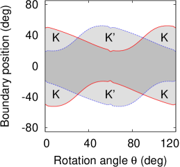
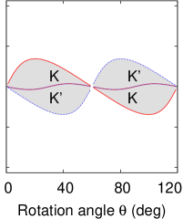
Figure 12: (Color online). Optimized single valley regions for 116.9 meV holes in MoTe₂. Solid red lines: $K$ transmission boundaries, dashed blue lines: $K^{\prime}$ boundaries. Light fill: single valley transmission, dark fill: two valley transmission. Left: same valley at $\pm$ incidence. Right: different valleys at $\pm$ incidence; in this case cut-offs similar to those in Fig. 7 occur very close to $\theta=0$, $60$ and $120^{\circ}$.

Fig. 3 shows single valley transmission of holes in MoTe₂. $K$ and $K^{\prime}$ are defined as in ref. Kormanyos13 and spin up holes are transmitted in the $K$ valley. The barrier width is 300 nm, as for BLG, and the transmission coefficients are qualitatively similar to those for BLG. However the cut-offs at the critical angles are much sharper than for BLG. The reason is that the evanescent wave decay lengths in TMDs are typically an order of magnitude smaller than in BLG. Consequently the transmission coefficients in the total external reflection regime are much smaller, typically $<10^{-27}$ at 0.1^∘ into this regime in MoTe₂.

MoTe₂ is the most favorable TMD as it has the largest single valley region widths of all the TMDs. Fig. 12 shows that the optimized region widths, $\sim 16.0-30.6^{\circ}$, are similar to those in BLG. The region widths of all the semiconducting TMDs are compared in the next sub-section.

VI.5 Comparison of Single Valley Regions in semiconducting TMDs

	MoS2	MoSe2	MoTe2	WS2	WSe2	WTe2
$\mathbf{k}\cdot\mathbf{p}$	121.7	112.2	116.9	97.3	95.2	114.2
ab-initio	125.3	116.9	117.7	108.3	108.1	129.2

Table 3: Hole Fermi energies in meV corresponding to hole densities of $3\times 10^{13}$ cm^-2 in MoX₂ and $1.5\times 10^{13}$ cm^-2 in WX₂.

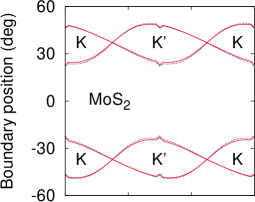
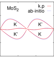
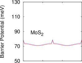
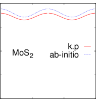
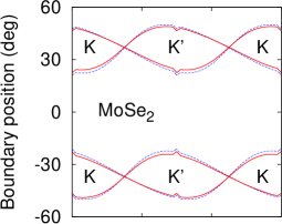
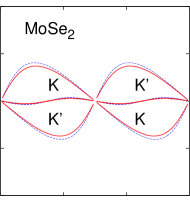
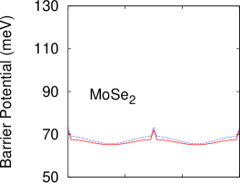
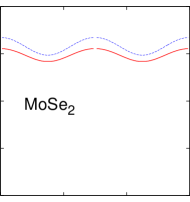
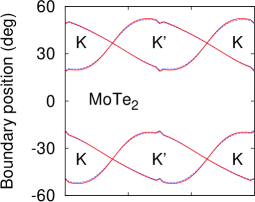
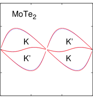
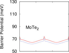
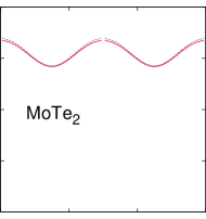
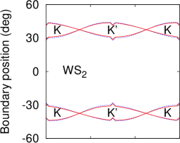
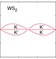
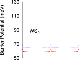
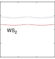
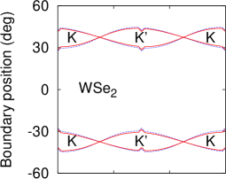
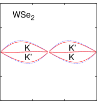
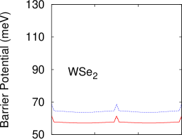
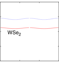
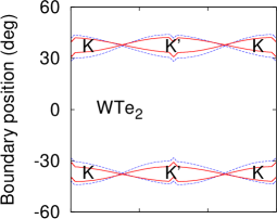
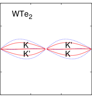
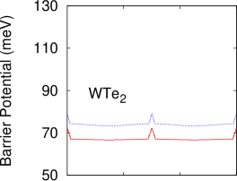
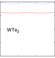
Figure 13: (Color online). Left two columns: single valley regions in the semiconducting TMDs (left side, same valley; right side, different valleys). Transmission of holes occurs between the $K$ and $K^{\prime}$ boundary lines in the indicated valleys. Right two columns: corresponding optimal barrier potentials (left side, same valley; right side, different valleys).

Region widths obtained from the $\mathbf{k}\cdot\mathbf{p}$ and ab-initio tight binding Hamiltonians are compared at constant hole density. The reason for working at constant density is that the density is proportional to the area enclosed by a constant energy contour. So when the comparison is done at constant density, differences in the region widths may be attributed to differences in the shape of the contour. This allows one to assess whether the $\mathbf{k}\cdot\mathbf{p}$ Hamiltonian reproduces trigonal warping accurately.

The hole density is taken to be $3\times 10^{13}$ cm^-2 in the Mo materials. However $E(\mathbf{k})$ varies more rapidly in the W materials so a significantly larger gate bias would be needed to achieve the same hole density as in the Mo materials. For this reason the density is taken to be $1.5\times 10^{13}$ cm^-2 in the W materials. The hole Fermi energies at which these densities occur are given in Table 3, relative to the edge of the upper spin split valence band.

Fig. 13 (left two columns) shows single valley region boundaries for all six semiconducting TMD monolayers. The boundaries computed with the $\mathbf{k}\cdot\mathbf{p}$ and ab-initio tight binding Hamiltonians typically agree to within 1.0-2.7^∘ for all materials except WTe₂. This suggests that the $\mathbf{k}\cdot\mathbf{p}$ Hamiltonian is reliable except in the case of WTe₂ so the transmission coefficients for MoTe₂ shown in Fig. 3 should also be reliable. In addition, Fig. 13 shows that the single valley region widths are largest in MoTe₂ so, as stated section VI.4, MoTe₂ is the most favorable TMD. This is consistent with ref. Habe15 in which the authors suggest the use of MoTe₂ to observe spin-dependent refraction, an effect that also depends on trigonal warping.

In the different-valley case, cut-offs occur as for BLG but only within about $1^{\circ}$ of $\theta=0$, $60$ and $120^{\circ}$. Hence single valley transmission in different valleys occurs in a much wider $\theta$ range than in BLG. The reason for this difference is that in TMDs the typical radial size of the barrier contour relative to the size of the contact contour is much smaller than in BLG. (For example, near the cut-off closest to $\theta=0^{\circ}$, the ratio of the barrier contour size to the contact contour size on the positive $k_{x}$-axis is 0.017 in MoTe₂ and 0.27 in BLG.) Hence in TMDs a larger rotation away from $\theta=30^{\circ}$ or $\theta=90^{\circ}$ is needed to take the end point of a propagating part around a corner of a contour. Thus the different-valley regions persist over a wider $\theta$ range in TMDs, for the energies considered here.

Fig. 13 (right two columns) shows the optimal potential barrier heights used to compute the single valley region boundaries shown in Fig. 13. As in BLG, the potentials needed for single valley regions in same and different valleys do not overlap and the potential has to be adjusted to get single valley regions of large width for all $\theta$. In addition, and as in BLG, the region widths calculated with a fixed $\theta$-independent potential, equal to the mid-range optimal potential are up to $\sim 20\%$ smaller than the optimized regions.

VI.6 Experimental Feasibility

The necessary experimental conditions are the same as for BLG: the material must be in the ballistic regime, the incident hole beam must be collimated and gates are needed to set the hole density and provide a barrier potential. The ballistic regime in monolayer TMDs has not yet been reached; the current experimental situation is detailed in section VII.2.1. The other two conditions are probably close to being satisfied. The MLG collimator Barnard17 simply consists of suitably shaped gates deposited on hBN encapsulated graphene. There seems to be no reason why similar gates should not be deposited on insulated TMDs, although two top gates or two collimators may be needed as the same-valley and different-valley cases occur at different angles of incidence. The bottom and top gates, that are needed to control the hole density and provide the barrier, resemble the gates used to make FETs and TMD FETs have been fabricated. For example n-FETs have been made from monolayer MoS₂ Baugher13 ; Radisavljevic13 , p-FETs from monolayer WSe₂ Fang12 and ambipolar FETs from monolayer MoTe₂ Larentis17 .

However the question of whether the hole density of $3\times 10^{13}$ cm^-2 used here can be achieved in MoTe₂ is open as the hole density in the ambipolar MoTe₂ FET has not been reported. Typical carrier densities in TMD FETs exceed about $10^{12}$ - $10^{13}$ cm^-2 and the hole density used here is slightly less than the maximum electron density reported in monolayer MoS₂ ($3.6\times 10^{13}$ cm^-2, Radisavljevic13 ). If this density cannot be achieved it would be possible to use a lower hole density which would require a lower hole Fermi level. However this would lead to reduced trigonal warping and narrower single valley region widths and hence require an incident hole beam of narrower width.

VII Possible realization of a valley polarizer

In sections V and VI we have shown that transmission of carriers through potential barriers in BLG and TMDs is valley asymmetric and single valley transmission occurs over a wide range of incidence angles. In this section we suggest these effects can be used to realize a valley polarizer.

We detail the minimum requirements for this device in section VII.1. Then in section VII.2 we examine factors which may affect the operating temperature and the accuracy of valley polarization. The maximum operating temperature is likely to be the maximum temperature at which ballistic transport occurs (VII.2.1). Thermally excited minority carriers could affect the polarization accuracy but only in BLG and their effect can be suppressed by raising the back gate voltage(VII.2.2). Because of the thermal spread of energies in the incident beam, the same-valley regime is most favorable for higher temperature operation (VII.2.3). The effect of in-plane electric fields is likely to be small (VII.2.4).

VII.1 Minimum requirements for a valley polarizer

The main requirement is a collimated beam of carriers in the ballistic regime. If a macroscopic contact was used instead of a collimator, it would probably supply carriers with valley symmetric and equal probability at each point on each energy contour. Then time reversal symmetry would ensure that the conductance is valley symmetric. However a collimator operating in the ballistic regime can be arranged to supply carriers only in the range of velocities where single valley transmission occurs and thus make a valley polarizer. The necessary collimator has been demonstrated in graphene Barnard17 and its beamwidth is $18^{\circ}$, similar to the minimum range widths in Figs. 7 and 12. Another requirement is to dispose of the reflected carriers which are in the undesired valley and could be backscattered from the edges of the 2D material and pass through the barrier. This can be done by putting grounded electrodes at the edges to absorb the undesired carriers. A similar absorber has been demonstrated as a key part of the collimator in ref. Barnard17 . The ballistic regime has been reached in BLG Cobaleda14 ; Nam17 ; Varlet14 ; Oka19 hence a BLG valley polarizer can be realized from components that have been demonstrated. In TMDs, the hole regime is experimentally accessible in monolayer MoTe₂ Larentis17 but ballistic transport in this material has not yet been investigated.

VII.2 Factors affecting temperature of operation and polarization accuracy

VII.2.1 Ballistic Transport

Ballistic transport in BLG at low temperature is well established experimentally Cobaleda14 ; Nam17 ; Varlet14 ; Oka19 but the maximum temperature for ballistic transport is not known. The authors of ref. Cobaleda14 investigated the temperature dependence of transport in hBN encapsulated BLG and found that ballistic transport occurs above a temperature-independent critical carrier density of $2.5\times 10^{11}$ cm^-2 up to 50 K, the maximum temperature used in the experiment. The authors of ref. Nam17 investigated transport in suspended BLG and found that ballistic transport occurs above a temperature-dependent critical density. The maximum experimental temperature was 70 K and the corresponding critical density is $\sim 2\times 10^{11}$ cm^-2. Hence the available experimental evidence suggests that ballistic transport in BLG occurs at least up to $\sim 50$ - $70$ K but further work is needed to determine the upper limit.

In the case of TMDs ballistic transport has been investigated only for electrons in MoS₂ English16 . The authors of this work observed the onset of ballistic transport at a device temperature of 175 K and suggested that the ballistic limit can be achieved. As the electron and hole masses are similar ($\sim 0.5$) in all the semiconducting TMDs Kormanyos15 , it is possible that ballistic transport of holes can be achieved. However there is no relevant data and further experimental investigations are needed.

In summary, the temperature dependence of ballistic transport may limit the maximum operating temperature of a valley polarizer but there is insufficient experimental evidence to estimate this temperature.

VII.2.2 Minority Carriers

Thermally excited minority carriers in the contacts could affect the valley polarization but the physics is different in BLG and TMDs.

In the case of BLG and the device model in V.2, the electron Fermi level is 56 meV and the layer potentials in the contacts are $\pm 14$ meV. The physics depends on the alignment of the bands in the contacts and underneath the top gate. From Fig. 8 it can be seen that for almost all $\theta$, the layer 1 potential under the top gate is $>14$ meV and the layer 2 potential is $>-14$ meV. Hence the top gate generates a barrier for electrons and a well for holes. This means that thermally excited holes in both valleys could flow underneath the top gate, leading to a reduction in valley polarization.

The magnitude of this effect depends on the thermal distribution of the holes. The Fermi function is equal to 0.01 when $E-E_{F}\sim 4.6k_{B}T$, where $E_{F}$ is the Fermi level, $T$ is the absolute temperature and $k_{B}$ is Boltzmann’s constant. This condition should give a rough approximation to the temperature at which the valley polarization is affected by a few %. For the device model in section V.2, the energy needed to create a hole is 70 meV and the corresponding temperature is $\sim 177$ K.

It should be possible to reduce the effect of the holes by increasing the back gate voltage. In the device model detailed in section V.2, the electron Fermi level becomes 105 meV if the back gate voltage is raised to 4000 mV, and the layer potentials in the contact become $\pm 31$ meV. Then the hole creation energy increases to 136 meV and the corresponding temperature is $\sim 343$ K. This shows it should be possible to overcome the effects of holes in BLG with a suitable device design.

In the case of TMDs, the band gap exceeds 1 eV so thermal excitation of carriers across the gap is unlikely to be significant at room temperature and beyond. However the effect of excitation across the spin split valence bands needs to be considered.

The holes in both of the spin split bands are subjected to the same potential barrier. In addition, $E(\mathbf{k})$ is similar for both spins. Hence the single valley regions for both spins are similar. Consequently the valley polarization should not be affected by minority spin holes. However the spin polarization could be affected.

Minority spin holes can be transmitted through the barrier only if their energy relative to the bottom of the minority spin band exceeds the barrier height. Creation of holes of this energy requires a thermal excitation of energy $2|\lambda|-E_{F}+V$ where $E_{F}$ is the hole Fermi energy in the majority spin band and $V$ is the barrier height. With $E_{F}=116.9$ meV and $V=66.55$ meV as for Fig. 3, this gives an energy of 164.65 meV and the corresponding temperature, obtained with the same criterion as for BLG, is 415 K.

In summary, minority carriers are unlikely to affect the spin and valley polarizations in TMDs and their effect on the valley polarization in BLG can be suppressed by increasing the back gate voltage.

VII.2.3 Thermal Spread of Energies in Incident Beam

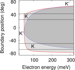
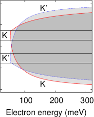
Figure 14: (Color online). Energy dependence of single valley regions in BLG. The potentials and top gate width are as for Fig. 2. Solid red lines: $K$ transmission boundaries, dashed blue lines: $K^{\prime}$ boundaries. Horizontal lines indicate the beam extent. Light fill: single valley transmission, dark fill: two valley transmission. Left: $\theta=17^{\circ}$ (same-valley case at $E=56$ meV). Right: $\theta=31^{\circ}$ (different-valley case at $E=56$ meV).

The single valley regions depend significantly on energy. Therefore at finite temperature the spread of energies in the incident beam could affect the valley polarization. To investigate this, the single valley region boundaries are computed as a function of energy at $\theta=17^{\circ}$ and $31^{\circ}$. Figs. 2 and 3 show that same-valley transmission occurs at $\theta=17^{\circ}$ when $E=56$ meV in BLG and $E=116.9$ meV in MoTe₂ while different-valley transmission occurs at the same energies when $\theta=31^{\circ}$. However Figs. 14 (BLG) and 15 (MoTe₂) confirm that the form of the transmission is energy-dependent.

In both materials there is a threshold energy equal to the barrier height. If $\phi_{c}$ is fixed and only the energy is varied, then in BLG at both angles and MoTe₂ at $31^{\circ}$, there is a critical energy where single valley transmission changes to transmission in both valleys (light fill changes to dark fill when the energy increases). This limits the maximum operating temperature.

To quantify this, a beam of width $18^{\circ}$ is indicated by the parallel, horizontal lines in the figures. Each pair of lines is centered on the angle that makes the threshold energy approximately equal to the Fermi energy, 56 meV for electrons in BLG and 116.9 meV for holes in MoTe₂. With this choice, carriers whose energy is significantly less than the Fermi energy are below the first threshold and are not transmitted. Then the maximum operating temperature is determined by the carrier population above the critical energy.

For example, in BLG at $31^{\circ}$ the critical energy at $\phi_{c}=-13.2^{\circ}$ is 61.7 meV and with the criterion used in section VII.2.2 this corresponds to a temperature of 14.4 K. For the $\phi_{c}=11.2^{\circ}$ line the temperature is 8.8 K. In MoTe₂ the equivalent temperatures are 86.8 K and 64.6 K. This suggests that the regime where single valley transmission occurs in different valleys at positive and negative incidence is not very suitable for high temperature operation.

The regime where the single valley transmission occurs in the same valley is much more suitable. In BLG at $\theta=17^{\circ}$, the critical energy at $\phi_{c}=-49^{\circ}$ corresponds to a temperature of 190 K. However the critical energy at $\phi_{c}=25.2^{\circ}$ corresponds to 27.5 K and generally in BLG the second threshold only occurs at high energy in one of the single valley regions. In MoTe₂ at $\theta=17^{\circ}$ there is no crossover to transmission in both valleys up to an energy of at least 377.5 meV. This is very favorable for high temperature operation. The physical reason for the different behavior of BLG and MoTe₂ is that in the energy range considered here, trigonal warping weakens with energy in BLG but strengthens with energy in TMDs.

In summary, the regime where single valley transmission occurs in the same valley at both positive and negative angles of incidence is very favorable for high temperature operation. However in BLG this is the case for only one of the single valley regions. Which one it is depends on $\theta$ as consequence of Eq. (39).

VII.2.4 In-plane Electric Fields

In-plane electric fields should deflect a collimated carrier beam and change the angle of incidence. This could cause loss of polarization if the incident beam is shifted away from a single valley region into a two valley region. However we estimate that this effect is likely to be small.

The magnitude of the effect depends on the experimental voltages and device dimensions. The Fabry-Perot interference experiments described in ref. Varlet14 were done with a source-drain bias of around 1 mV over a distance of around 1-3 $\mu$m while the collimation experiments described in ref. Barnard17 probably involved smaller fields. Hence 1000 Vm^-1 is taken to be an upper limit to the in-plane field.

To estimate the deflection, the field is taken to be normal to the barrier and classical trajectories for a charged particle with energy-momentum relation $E(\mathbf{p}/\hbar)$ are computed for each valley, where $E(\mathbf{k})$ is the band energy. The results show that the incident beam can undergo a small deflection towards the two valley region. The deflection angle depends on $\theta$ but is only $\sim 0.1$ - $0.2^{\circ}$ for BLG and only $\sim 0.05$ - $0.14^{\circ}$ for MoTe₂. This is small compared to single valley region widths and suggests the effect of in-plane electric fields will be small under typical experimental conditions.

VIII Detection of valley polarization

Valley polarization can be detected via the valley Hall effect Xiao07 ; Sui15 ; Shimazaki15 and it has been suggested that two valley polarizers of opposite polarity can block current Rycerz07 . When the polarizers are made from barriers, the blockage is exact because of the symmetry relation, Eq. (38), between the transmission coefficients of two barriers with a relative rotation angle of $\pi/3$.

This relation allows a polarization detector to be made from two identical and inversion symmetric barriers in series, with a relative rotation of $\pm\pi/3$ (Fig. 16). When the two single valley regions are in the same valley at positive and negative $\phi_{c}$, as in Fig. 2 (left), Eq. (38) guarantees that the second barrier transmits in the opposite valley to the first barrier. Hence the barrier pair blocks current and can be used like a pair of Polaroid filters to demonstrate valley polarization.

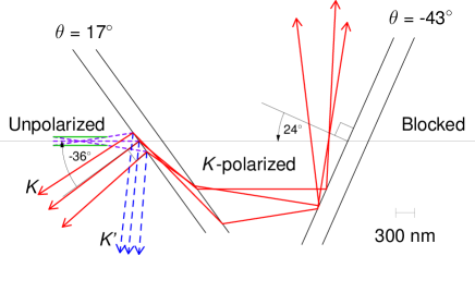
Figure 16: (Color online). Example of current blocking by two barriers. Sloping lines indicate barrier edges, the horizontal feint line is the optic axis and the short parallel lines (green) represent the collimator. Other lines show the current directions at the center and edges of each electron beam. Short dashed lines (purple): unpolarized incident current; solid lines (red): $K$ polarized; long dashed lines (blue): $K^{\prime}$ polarized. For clarity, current paths that enter the collimator from the left are not shown. Beam center reflection coefficients at the first barrier: 100% in $K^{\prime}$ and 5.5% in $K$.

In practice, this requires that two more conditions are satisfied. The first is that the current that is transmitted through the first barrier should be incident on the second barrier at an angle within the single valley range for that barrier. As the two barriers must have a relative rotation of $\pm 60^{\circ}$ to swap the valleys, the angles of incidence on the two barriers differ by $\mp 60^{\circ}$. To satisfy this condition, the angles of incidence in the two single valley regions should differ by about $60^{\circ}$. This is the case only in part of the $\theta$ range.

The second condition is that the reflected current from the front edge of the second barrier is not incident on the back edge of the first barrier. If this condition is not satisfied, multiple reflection between the two barriers could occur and this could change the transmission characteristics of the barrier combination. This can be prevented by adjusting the barrier lengths and separation so that the current reflected from the second barrier does not reenter the first barrier.

To demonstrate that the two conditions can be satisfied, ray tracing is used to compute the current paths through the two barriers for the case of BLG and $\theta=17^{\circ}$. The angles of reflection and refraction are obtained from the BLG band structure and the incident beam width is taken to be $18^{\circ}$. The current paths are shown in Fig. 16 and it is clear that the two conditions are satisfied. The angles of incidence on each barrier fall within the single valley ranges as can be checked by looking at Figs. 2 and 7. In addition, the current reflected from the second barrier clearly passes out of the region between the barriers. This suggests that the current blocking is experimentally observable, at least at one value of $\theta$.

The full $\theta$ range in which current blocking should be observable is probably somewhat smaller than the $\theta$ range of the same valley regions (Fig. 7, left). These regions become narrower and vanish as $\theta$ approaches $30^{\circ}\pmod{120^{\circ}}$ and $90^{\circ}\pmod{120^{\circ}}$. A significant fraction of the $\theta$ range should still be available but how much depends on the experimental conditions and extensive ray tracing calculations for the full range of $\theta$ angles and beam widths would be needed to determine this.

The current paths in Fig. 16 differ qualitatively from the paths of optical rays passing through a refractive medium. In particular, the order of the paths reverses at the first barrier, for example the top path on the entrance side becomes the bottom path on the exit side. The reason is that the $\mathbf{k}$-vectors of the states involved are by chance close to points of inflection on the barrier energy contour. Between the points of inflection, $\phi_{v}$ increases when $\phi_{k}$ decreases (see Fig. 4 (lower) for an example) and this leads to the reversed order. Another difference is that the angle of reflection is not equal to the angle of incidence when the energy contours are warped. This has a significant effect on the current paths reflected from the second barrier.

IX Discussion

Valley asymmetric transmission through a potential barrier in BLG and TMDs inevitably occurs because of the low symmetry of the total Hamiltonian. However it may be necessary to use additional physics to make the valley asymmetry large. We have suggested the use of total external reflection but this is not the only approach. For example, the valley asymmetry is enhanced in barriers with broken inversion symmetry Maksym18 .

The large valley asymmetry found in this work occurs because trigonal warping leads to a large difference in the critical angles for total external reflection in the two valleys. This results in single valley transmission over a wide range of incidence angles and enables a valley polarized incident current to be split into reflected and transmitted currents with opposite valley polarization. A valley polarizer can be realized in BLG by arranging for a collimated beam of carriers to be incident in one of the single valley regions. The same arrangement in TMDs forms a spin and valley polarizer. The barrier potential can be adjusted to ensure that single valley region widths are similar to or exceed the beam width of a MLG electron collimator that has already been fabricated Barnard17 . In addition, we have shown that the transmitted valley swaps when a barrier is rotated by $\pm\pi/3^{\circ}$ with respect to the crystallographic axes. This allows two barriers with a relative rotation of $\pm\pi/3^{\circ}$ to be used like Polaroid filters to demonstrate valley polarization.

Our investigations show that the proposed valley polarizer appears to be experimentally feasible and should have some advantages. First, the polarizer is relatively immune to the crystallographic orientation of the barrier because the top gate voltage can be adjusted to optimize the single valley region widths. Secondly, the current on the exit side flows only in the desired valley so there is no need for additional components to collect the desired current stream. However some uncertainty about the feasibility remains because the trigonal warping parameters in BLG are not known reliably and accurate experimental values are desirable. Experimental studies to determine the conditions for ballistic transport in BLG and TMDs, particularly the temperature range, are also needed. Further theoretical work should await these experimental developments.

The inevitability of valley asymmetry is expected to be relevant to other applications and materials. It may be possible to use switchable pairs of spin filters to inject spin-polarized holes into a TMD pn-junction and hence make a polarized light emitting diode with electrically controllable photon polarization. In addition, the strong $\theta$ dependence of the transmission may be useful for determining the crystallographic orientation of the 2D material. Beyond BLG and TMDs, the total Hamiltonian of any 2D material in the presence of a gate should have low symmetry and transmission through a gate-induced barrier should be strongly $\theta$-dependent when the constant energy contours are not circular. Further afield, the present work may be relevant to valley photonic metamaterials Garcia08 ; Dong17 .

- (1) S. A. Vitale, D. Nezich, J. O. Varghese, P. Kim, N. Gedik, P. Jarillo-Herrero, D. Xiao and M. Rothschilde, Small 14, 1801483 (2018).
- (2) F. Amet and G. Finkelstein, Nat. Phys. 11, 989 (2015).
- (3) F. Bussolotti, H. Kawai, Z. E. Ooi, V. Chellappan, D. Thian, A. L. C. Pang and K. E. J. Goh, Nano Futures 2, 032001 (2018).
- (4) J. R. Schaibley, H. Yu, G. Clark, P. Rivera1, J. S. Ross, K. L. Seyler, W. Yao and X. Xu, Nat. Rev. Mat. 1, 16055 (2016).
- (5) Y. P. Shkolnikov, E. P. De Poortere, E. Tutuc and M. Shayegan, Phys. Rev. Lett. 89, 226805 (2002).
- (6) O. Gunawan, B. Habib, E. P. De Poortere and M. Shayegan, Phys. Rev. B 74, 155436 (2006).
- (7) K. Takashina, Y. Ono, A. Fujiwara, Y. Takahashi and Y. Hirayama, Phys. Rev. Lett. 96, 236801 (2006).
- (8) Z. Zhu, A. Collaudin, B. Fauqué, W. Kang and K. Behnia, Nat. Phys. 8, 89 (2012).
- (9) A. Rycerz, J. Tworzydło and C. W. J. Beenakker, Nat. Phys. 3, 172 (2007).
- (10) D. Xiao, W. Yao and Q. Niu, Phys. Rev. Lett, 99 236809 (2007).
- (11) J. L. Garcia-Pomar, A. Cortijo and M. Nieto-Vesperinas Phys. Rev. Lett. 100, 236801 (2008).
- (12) D. S. L. Abergel and T. Chakraborty, Appl. Phys. Lett. 95, 062107 (2009).
- (13) J. M. Pereira Jr, F. M. Peeters, R. N. Costa Filho and G. A. Farias, J. Phys: Condens. Matter 21 045301 (2009).
- (14) H. Schomerus, Phys. Rev. B 82, 165409 (2010).
- (15) C. Park, Solid State Commun. 152, 2018 (2012).
- (16) C. Park, J. Appl. Phys. 118, 244301 (2015).
- (17) F. W. Chen, M. Y. Chou, Y. R. Chen and Y. S. Wu, Phys. Rev. B 94, 075407 (2016).
- (18) A. Cresti, G. Grosso and G. P. Parravicini, Phys. Rev. B 77, 233402 (2008).
- (19) G. Tkachov, Phys. Rev. B 79, 045429 (2009).
- (20) D. Gunlycke and C. T. White, Phys. Rev. Lett. 106, 136806 (2011).
- (21) Z. Wu, F. Zhai, F. M. Peeters, H. Q. Xu and K. Chang, Phys. Rev. Lett. 106, 176802 (2011).
- (22) M. Koshino, Phys. Rev. B 88, 115409 (2013).
- (23) See Fig. 2 of ref. Garcia08 for an example.
- (24) A. W. Barnard, A. Hughes, A. L. Sharpe, K. Watanabe, T. Taniguchi and D. Goldhaber-Gordon, Nat. Commun. 8, 15418 (2017).
- (25) T. Low and F. Guinea, Nano Lett. 10, 3551 (2010).
- (26) C. Péterfalvi, L. Oroszlány, C. J. Lambert and J. Cserti, New Journal of Physics. 14, 063028 (2012).
- (27) F. Zhang, A. H. MacDonald and E. J. Mele, PNAS 110, 10546 (2013).
- (28) Si-Yu Li, Ying Su, Ya-Ning Ren and Lin He, Phys. Rev. Lett. 124, 106802 (2020).
- (29) Carolin Gold, Angelika Knothe, Annika Kurzmann, Aitor Garcia-Ruiz, Kenji Watanabe Takashi Taniguchi, Vladimir Fal’ko, Klaus Ensslin and Thomas Ihn, Phys. Rev. Lett. 127, 046801 (2021).
- (30) Hao Chen, Pinjia Zhou, Jiawei Liu, Jiabin Qiao, Barbaros Oezyilmaz and Jens Martin, Nat. Commun. 11, 1202 (2020).
- (31) K. F. Mak, K. L. McGill, J. Park and P. L. McEuen, Science 344, 1489 (2014).
- (32) X. X. Zhang, Y. Lai, E. Dohner, S. Moon, T. Taniguchi, K. Watanabe, D. Smirnov and T. F. Heinz, Phys. Rev. Lett. 122, 127401 (2019).
- (33) T. Habe and M. Koshino, Phys. Rev. B 91, 201407(R) (2015).
- (34) T. C. Hsieh, M. Y. Chou and Y. S. Wu, Phys. Rev. Mat. 2, 034003 (2018).
- (35) E. McCann and M. Koshino, Rep. Prog. Phys. 76, 056503 (2013).
- (36) A. Kormányos, V. Zólyomi, N. D. Drummond, P. Rakyta, G. Burkard and V. I. Fal’ko, Phys. Rev. B 88, 045416 (2013).
- (37) H. Rostami, A. G. Moghaddam and R. Asgari, Phys. Rev. B 88 085440 (2013).
- (38) E. McCann, Phys. Rev. B 74, 161403(R) (2006).
- (39) Outside this range four propagating states or four evanescent states may occur.
- (40) D. Xiao, G. B. Liu, W. Feng, X. Xu and W. Yao, Phys. Rev. Lett, 108 196802 (2012).
- (41) G. B. Liu, W. Y. Shan, Y. Yao, W. Yao and D. Xiao, Phys. Rev. B 88, 085433 (2013).
- (42) P. A. Maksym, Surf. Rev. Lett., 4, 513 (1997).
- (43) P. A. Maksym and H. Aoki, in preparation.
- (44) P. A. Maksym and H. Aoki, in preparation.
- (45) P. Goswami, Graphene 2, 88 (2013).
- (46) G. Giovannetti, P. A. Khomyakov, G. Brocks, P. J. Kelly and J. van den Brink, Phys. Rev. B 76, 073103 (2007); L. Ci, L. Song, C. Jin, D. Jariwala, D. Wu, Y. Li, A. Srivastava, Z. F. Wang, K. Storr, L. Balicas, F. Liu, and P. M. Ajayan, Nat. Mater. 9, 430 (2010); C. Yelgel and G. P. Srivastava, Appl. Surf. Sci. 258, 8342 (2012).
- (47) A. Varlet, M. H. Liu, V. Krueckl, D. Bischoff, P. Simonet, K. Watanabe, T. Taniguchi, K. Richter, K. Ensslin and T. Ihn, Phys. Rev. Lett. 113, 116601 (2014).
- (48) A. Ramasubramaniam, D. Naveh and E. Towe, Nano Lett. 11, 1070 (2011).
- (49) S. Predin, P. Wenk and J. Schliemann, Phys. Rev. B 93, 115106 (2016).
- (50) F. Xia, D. B. Farmer, Y. Lin and P. Avouris, Nano Lett., 10, 715 (2010).
- (51) H. Miyazaki, K. Tsukagoshi, A. Kanda, M. Otani and S. Okada, Nano Lett., 10, 3888 (2010).
- (52) J. Yan and M. S. Fuhrer, Nano Lett., 10, 4521 (2010).
- (53) C. Cobaleda, S. Pezzini, E. Diez and V. Bellani, Phys. Rev. B 89 121404(R) (2014).
- (54) Y. Nam, D. Ki, D. Soler-Delgado and A. F. Morpurgo, Nat. Phys. 13 1207 (2017).
- (55) T. Oka, S. Tajima, R. Ebisuoka, T. Hirahara, K. Watanabe, T. Taniguchi and R. Yagi, Phys. Rev. B 99 035440 (2019).
- (56) A. Kormányos, G. Burkard, M. Gmitra, J. Fabian, V. Zólyomi, N. D. Drummond and V. Fal’ko, 2D Mater 2, 022001 (2015).
- (57) A. Jain, S. P. Ong, G. Hautier, W. Chen, W. D. Richards, S. Dacek, S. Cholia, D. Gunter, D. Skinner, G. Ceder and K. A. Persson, APL Materials 1, 011002 (2013).
- (58) C. D. English, K. K. H. Smithe, R. Xu and E. Pop, Proc. 2016 IEEE Int. Elect. Dev. Meeting (IEDM) (2016).
- (59) B. W. H. Baugher, H. O. H. Churchill, Y. Yang, and P. Jarillo-Herrero, Nano Lett. 13, 4212 (2013).
- (60) B. Radisavljevic and A. Kis, Nat. Mat. 12, 815 (2013).
- (61) H. Fang, S. Chuang, T. C. Chang, K. Takei, T. Takahashi and A. Javey, Nano Lett. 12, 3788 (2012).
- (62) S. Larentis, B. Fallahazad, H. Movva, K. Kim, A. Rai, T. Taniguchi, K. Watanabe, S. K. Banerjee and E. Tutuc, ACS Nano 11, 4832 (2017).
- (63) M. Sui, G. Chen, L. Ma, W. Shan, D. Tian, K. Watanabe, T. Taniguchi, X. Jin, W. Yao, D. Xiao and Y. Zhang, Nat. Phys. 11, 1027 (2015).
- (64) Y. Shimazaki, M. Yamamoto, I. V. Borzenets, K.Watanabe, T. Taniguchi and S. Tarucha, Nat. Phys. 11, 1032 (2015).
- (65) J. Dong, X. Chen, H. Zhu, Y. Wang and X. Zhang, Nat. Mat. 16, 298 (2017).