NGTS-8b and NGTS-9b: two non-inflated hot-Jupiters

Abstract

We report the discovery, by the Next Generation Transit Survey (NGTS), of two hot-Jupiters NGTS-8b and NGTS-9b. These orbit a $V\,=\,13.68$ K0V star ($T_{eff}$ = $5241\pm 50$ K) with a period of $2.49970$ days, and a $V\,=\,12.80$ F8V star ($T_{eff}$ = $6330\pm 130$ K) in $4.43527$ days, respectively. The transits were independently verified by follow-up photometric observations with the SAAO 1.0-m and Euler telescopes, and we report on the planetary parameters using HARPS, FEROS and CORALIE radial velocities. NGTS-8b has a mass, $0.93\,^{+0.04}_{-0.03}$ M_J and a radius, $1.09\pm 0.03$ R_J similar to Jupiter, resulting in a density of $0.89\,^{+0.08}_{-0.07}$ g cm^-3. This is in contrast to NGTS-9b, which has a mass of $2.90\pm 0.17$ M_J and a radius of $1.07\pm 0.06$ R_J, resulting in a much greater density of $2.93^{+0.53}_{-0.49}$ g cm^-3. Statistically, the planetary parameters put both objects in the regime where they would be expected to exhibit larger than predicted radii. However, we find that their radii are in agreement with predictions by theoretical non-inflated models.

1 Introduction

Hot-Jupiters are giant gas exoplanets similar to Jupiter, but with a shorter orbital period, inferior to 10 days. While rare, these planets are the easiest to detect from ground-based surveys due to their relatively deep transits ($\sim 1\%$), their large radial velocity (RV) signals, and their short periods, which make hot-Jupiters important targets in order to understand the structure, composition and evolution of planetary systems.

From the currently observed population of exoplanets with known radii, masses and orbital distances, the evolution of planetary radii has been modelled (e.g. Fortney et al. 2007; Baraffe et al. 2008). These models, where the effects of stellar irradiation and heavy element cores are included, agree with observations at low stellar irradiation. However, the observed radii of highly irradiated gas giants are discrepant with theoretical expectations. For instance, at fluxes greater than $2\times 10^{5}$ W m^-2 (Miller & Fortney 2011; Demory & Seager 2011) the gas giants are increasingly found with anomalously large radii. This is the case for the hot-Jupiters WASP-17 b, WASP-121 b and Kepler-435 b, which all have measured radii R > 1.8 R_J(Anderson et al. 2011; Almenara et al. 2015; Delrez et al. 2016). A number of possible mechanisms have been postulated to explain these inflated planetary radii including kinetic heating (Guillot & Showman, 2002), enhanced atmospheric opacities (Burrows et al., 2007), double diffusive convection (Chabrier & Baraffe, 2007), Ohmic heating through magnetohydrodynamic effects (Batygin & Stevenson 2010; Perna et al. 2010; Wu & Lithwick 2012; Ginzburg & Sari 2016), tidal dissipation (Bodenheimer et al. 2001; Bodenheimer et al. 2003; Arras & Socrates 2010; Jermyn et al. 2017) and vertical advection of potential temperature (Youdin & Mitchell 2010; Tremblin et al. 2017). However, the exact mechanisms responsible are still, as yet, unidentified and the problem remains unsolved. In order to perform robust statistical studies of hot-Jupiter radii and constrain the dominant ‘inflation’ mechanisms at work (e.g. as done by Sestovic et al. 2018) we need to increase the sample of planets spanning a range of planetary masses, radii, stellar irradiation levels, as well as planetary system ages.

In this paper we present two hot-Jupiters that appear to be non-inflated, despite being highly irradiated with an incident flux greater than $2\times 10^{5}$ W m^-2 (like many inflated planets). In §2, the NGTS discovery data is described. §3 explains the photometric follow-up campaigns and §4 reports the mass determination via RV monitoring from spectroscopy. §5 details the analysis of the stellar parameters, presents the stellar activity and its relation with the stellar rotation and shows the global modelling process to characterize the planets. §6 presents an investigation regarding the incident flux, the planetary mass and the radius. Finally we finish with our conclusions in §7.

2 Discovery Photometry From NGTS

The Next Generation Transit Survey (NGTS), operating since early 2016, is a wide-field transit survey located at ESO’s Paranal Observatory in Chile, whose primary goal is to discover Neptune-sized or bigger exoplanets. NGTS has a fully robotized array of twelve 20 cm Newtonian telescopes, and each telescope is equipped with 2K$\times$2K e2V deep-depleted Andor IKon-L CCD cameras with 13.5 µm pixels and an instantaneous field of view of 8 deg². For a description of this facility and its capabilities, optimised for detecting planets, we refer the reader to Wheatley et al. (2018). NGTS has already detected 4 hot-Jupiters: NGTS-1b (Bayliss et al., 2018), NGTS-2b (Raynard et al., 2018), NGTS-3Ab (Günther et al., 2018) and NGTS-6b (Vines et al., 2019). Here we report the latest hot-Jupiter discoveries from NGTS: NGTS-8b and NGTS-9b.

NGTS-8 was observed using a single NGTS camera (#811) over a 227 night baseline between the 21st of April 2016 and the 3rd of December 2016. NGTS-9  was also observed using a single camera (#806) over a 234 night baseline between the 8th of October 2016 and the 29th of May 2017. A total of 177 799 and 167 933 images were obtained, respectively, each with an exposure time of $10$ s. These data were taken using the custom NGTS filter (520 – 890 nm) (Wheatley et al., 2018) and the telescope was auto-guided using an improved version of the DONUTS auto-guiding algorithm (McCormac et al., 2013). The data were reduced and aperture photometry was extracted using the CASUTools photometry package. A total of 177120 and 166043 valid data-points were extracted from the raw images and then de-trended for nightly trends, such as atmospheric extinction, using our implementation of the SysRem algorithm (Tamuz et al., 2005).

Both datasets were searched for transit-like signals using orion, an optimized implementation of the box-least-squares (BLS) fitting algorithm (Collier Cameron et al., 2006). A 1.6% deep transit signal was detected at a period of $2.49970$ days for the K0V star, NGTS-8, and a 0.6% deep transit signal at $4.43527$ days for the F8V star, NGTS-9. These periods were distinguished from other aliases using the photometry and spectroscopy follow-up – see Section 3 and Section 4 for details. The detrended NGTS data for the two stars, phase-folded on the planetary orbital periods, are shown in Figure 1 and Figure 2. A sample of the NGTS reduced photometric measurements are presented in Table 1 and Table 2, with the full data available electronically from the journal.

The NGTS data were searched for signs that would indicate that the planetary candidates were false positives. No evidence for a secondary eclipse or out-of-transit variations indicating an eclipsing binary system were identified in the NGTS light curves of the two stars. However, for both sources, some stars were found to be in close proximity to our targets. Using Gaia  we confirmed that these nearby stars did not appreciably dilute the light from NGTS-8 or NGTS-9, and also confirmed that NGTS-8 and NGTS-9 were not giants stars – see Section 5.1.1 for details. Based on the NGTS detection, NGTS-8 and NGTS-9 were followed-up with further photometry and spectroscopy to confirm the planetary nature of the system and to measure the planetary parameters, which we report on in the next section.

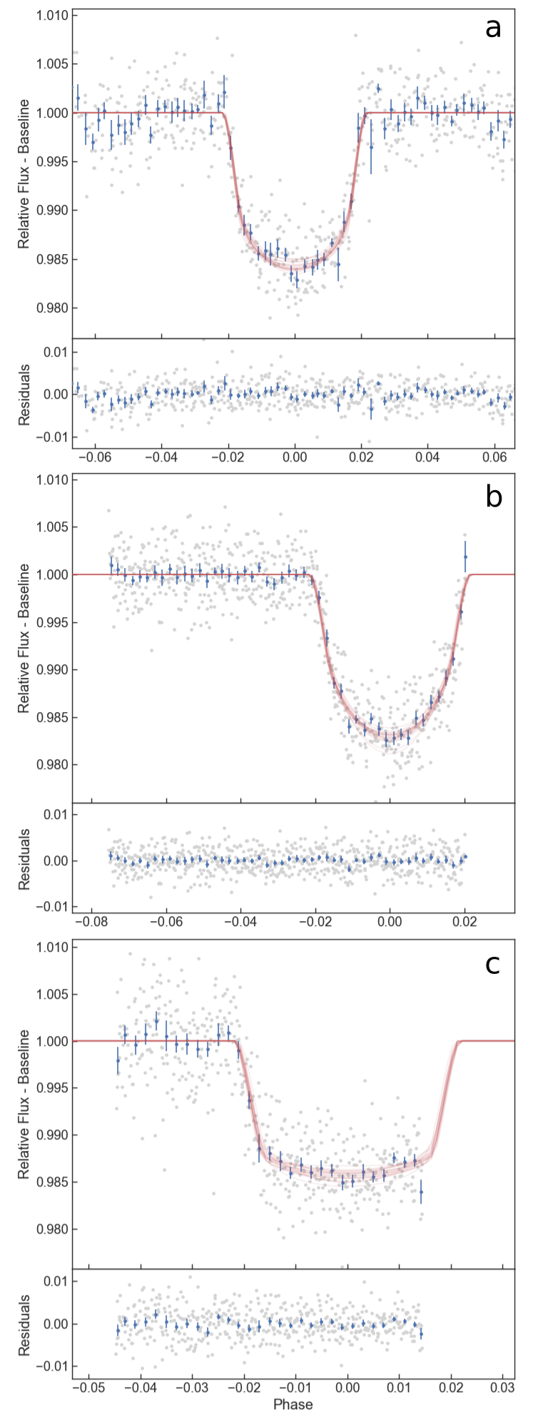
Figure 1: From top to bottom: Figure 1.a represents the NGTS discovery light curve of NGTS-8b with residuals, phase-folded on the orbital period and zoomed on the transit. Figure 1.b represnts the ingress and mid-transit of NGTS-8b observed with SAAO, with residuals. Figure 1.c represents the ingress and mid transit of NGTS-8b observed with Euler, with residuals. For all the plots, the blue data points are binned every 7 min to aid visualisation. The red lines show 20 light curve models generated from randomly drawn posterior samples of the allesfitter fit.

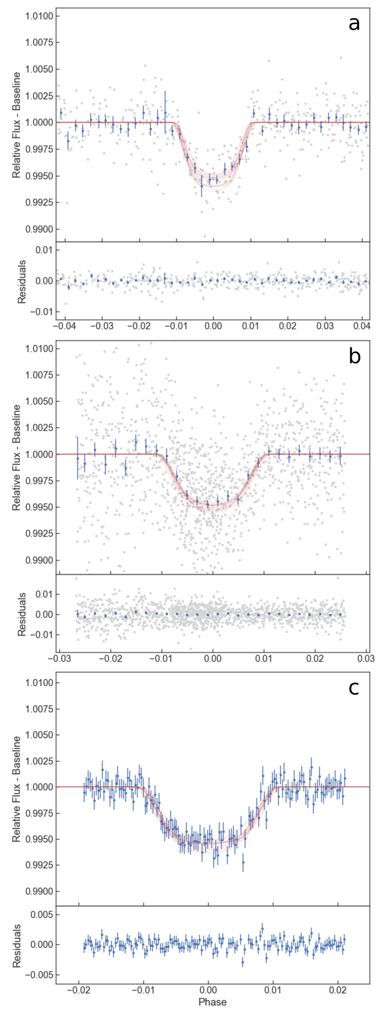
Figure 2: From top to bottom: Figure 2.a represents the NGTS discovery light curve of NGTS-9b with residuals, phase-folded on the orbital period and zoomed on the transit. Figure 2.b represents the full transit of NGTS-9b observed with SAAO, with residuals. This image uses night 20181221, where ingress and mid-transit can be seen, and night 20190103, with mid-transit and egress. For both figures, the blue data points are binned every 10 min to aid visualisation. Figure 2.c represents the full transit of NGTS-9b observed with Euler, with residuals. The data was taken on a 100sec cadence, shown in blue. For all the plots, the red lines show 20 light curve models generated from randomly drawn posterior samples of the allesfitter fit.

Table 1: A sample of the photometric data of NGTS-8 from NGTS, SAAO and Eulercam. The full dataset is available electronically from the journal.

Time	Relative	Flux	Filter	Instrument
(BJD-2450000)	flux	error
7499.8655	1.0179	0.0221	NGTS	NGTS
7499.8657	1.0320	0.0221	NGTS	NGTS
7499.8658	1.0016	0.0220	NGTS	NGTS
7499.8660	0.9964	0.0220	NGTS	NGTS
7499.8661	0.9911	0.0220	NGTS	NGTS
7499.8663	0.9995	0.0220	NGTS	NGTS
7499.8664	0.9892	0.0220	NGTS	NGTS
7499.8666	1.0054	0.0220	NGTS	NGTS
7499.8667	0.9910	0.0219	NGTS	NGTS
7499.8669	0.9901	0.0219	NGTS	NGTS
…	…	…	…	…

Table 2: A sample of the photometric data of NGTS-9 from NGTS, SAAO and Eulercam. The full dataset is available electronically from the journal.

Time	Relative	Flux	Filter	Instrument
(BJD-2450000)	flux	error
7669.8612	0.9871	0.0087	NGTS	NGTS
7669.8614	1.0027	0.0087	NGTS	NGTS
7669.8617	0.9919	0.0087	NGTS	NGTS
7669.8618	0.9848	0.0087	NGTS	NGTS
7669.8620	1.0107	0.0087	NGTS	NGTS
7669.8621	1.0014	0.0087	NGTS	NGTS
7669.8623	0.9956	0.0087	NGTS	NGTS
7669.8624	1.0167	0.0087	NGTS	NGTS
7669.8626	1.0076	0.0087	NGTS	NGTS
7669.8627	1.0000	0.0087	NGTS	NGTS
…	…	…	…	…

Table 3: A summary of the follow-up photometry of NGTS-8 and NGTS-9.

Night	Instrument	Target	Nimages	Exptime	Binning	Filter	Comment
				(seconds)	(X$\times$Y)
20170717	Shoc’n’awe	NGTS-8b	676	30	$4\times 4$	z’	shown in Figure 1.b
20170718	Shoc’n’awe	NGTS-8b	606	60	$4\times 4$	z’	no transit observed
20170821	Eulercam	NGTS-8b	502	12	$1\times 1$	IC	shown in Figure 1.c
20181221	Shoc’n’awe	NGTS-9b	550	20	$4\times 4$	$I$	shown in Figure 2.b
20190103	Shoc’n’awe	NGTS-9b	648	20	$4\times 4$	$I$	shown in Figure 2.b
20190112	Eulercam	NGTS-9b	134	100	$1\times 1$	RG	shown in Figure 2.c

3 Follow-up Photometry

3.1 SAAO photometry

Follow-up photometry of NGTS-8 was obtained with the 1.0 m Elizabeth telescope at the South African Astronomical Observatory (SAAO) on 2017 July 17 and 2017 July 18, utilising the frame-transfer CCD Sutherland High-speed Optical Camera "SHOC’n’awe" (Coppejans et al., 2013, SHOC).

With a pixel scale of 0.167 arcsec/pixel, the SHOC cameras on the 1 m telescope were binned $4\times 4$ pixels in the X and Y directions. The field of view of its instruments is $2.85\arcmin\times 2.85$′. This allow to observe simultaneously the target and a comparison star of similar brightness for differential photometry. The data, obtained using a $z^{\prime}$ filter with an exposure of 30 s, were bias and flat field corrected. This was performed in python using the standard procedure with the CCDPROC package (Craig et al., 2015). Then, using the ‘SEP’ package (Barbary, 2016), the aperture photometry of both the target and the comparison star were extracted. Finally, the sky background was measured and substracted using the SEP background map.

We also obtained two follow-up light curves of NGTS-9 on 2018 December 21 and 2019 January 30, with the same telescope and instrument set-up as described above. This time the data were obtained with an $I$ filter and an exposure time of 20 s. The data were reduced with the local SAAO SHOC pipeline, which is driven by python scripts running iraf tasks (pyfits and pyraf), and incorporating the usual bias and flat-field calibrations. Aperture photometry was performed using the Starlink package autophotom. For the first observation of NGTS-9 we used a 4 pixel radius aperture that maximised the signal/noise, and the background was measured in an annulus surrounding this aperture with inner and outer radii of 7 and 9 pixels, respectively. Two comparison stars were then used to perform differential photometry on the target. The 2019 January 30 observation was obtained in slightly poorer seeing conditions, and we therefore utilised a 6 pixel aperture, a correspondingly larger background annulus, and only one comparison star for differential photometry.

The transits of these two exoplanets observed from SAAO are shown in Figures 1.b and 2.b. Regarding NGTS-8, only a partial transit was observed with SAAO. For NGTS-9, 2 nights were combined: night 20181221, where ingress and mid-transit were seen, and night 20190103, where mid-transit and egress were seen. While only partial transits were observed, these SAAO data were able to confirm the transits and the consistency of the transit depths and were used to revise the orbital ephemerides for subsequent follow-up observations. In particular, the 2017 July observations of NGTS-8 were helpful in confirming the orbital period and ruling out aliases of similar power in the original NGTS data.

3.2 Eulercam

We also observed both objects with Eulercam (Lendl et al., 2012) on the 1.2 m Euler Telescope at La Silla Observatory. NGTS-8 was observed on the 21st of August 2017, 502 exposures were acquired using the Cousins-I filter, an exposure time of 12 s and a defocus of 0.05 mm. NGTS-9 was observed on the 12th of January 2019. We acquired 134 images using the Gunn-R filter, a 100 s exposure time and no defocus. For both target, their data were reduce using the standard procedure of bias subtraction and flat field correction. The aperture photometry as well as x- and y-position, FWHM, airmass and sky background of the target star were extracted using the PyRAF implementation of the phot routine. The comparison stars and the photometric aperture radius were carefully chosen in order to reduce the RMS in the scatter out of transit.

Using both follow-up photometry for the 2 stars, we can conclude that the nearby stars did not blend with the two targets. The Euler data for the two stars are shown in Figures 1.c and 2.c. Regarding NGTS-8, only a partial transit was observed with Euler. Concerning NGTS-9, the full transit was observed, with some systematics that were removed using a Gaussian process. Again, these data confirm the transits as we see the ingress or the full transit around the predicted times.

4 Spectroscopy

4.1 NGTS-8

NGTS-8 was observed with the HARPS spectrograph (Mayor et al., 2003) on the ESO 3.6 m telescope at La Silla Observatory, Chile, between the 5th of August 2017 and the 28th of October 2017 under programmes 099.C-0303 and 0100.C-0474. We used the high-efficiency mode, EGGS, due to the faintness of the host star and large expected RV amplitude. The exposure times for each spectrum varied between 1800 and 1200 s resulting in a signal-to-noise (SNR), measured around 550 nm, of 10-15 per exposure. The standard HARPS data reduction software (DRS) was used to measure the RVs of NGTS-8 at each epoch. This was done via cross-correlation with a K0 binary mask.

Three additional spectra were obtained with FEROS (Kaufer & Pasquini, 1998), mounted on the MPG 2.2 m telescope at La Silla Observatory, Chile, on the 20th and 21st of August 2017. All spectra were obtained with an exposure time of 1800 s, and the data were reduced using the FEROS routine of the CERES pipeline (Brahm et al., 2017). CERES also performed a radial velocity extraction, by cross-correlating the spectra with a G2 binary mask. The resulting SNR of the spectra, taken around 550 nm per resolution element, was around 45.

The RVs from both HARPS and FEROS are listed in Table 4, along with their associated error, FWHM and bisector span. While not presented in this table, the error on the BIS and on the FWHM were calculated using the same standard treatment as done previously (West et al., 2018). The errors for the BIS and for the FWHM are set to equal twice the error and 2.3548 times the error on the RV, respectively. The RV measurements of NGTS-8, shown phase folded in Figure 3, are in phase with the period detected by orion, with a semi-amplitude of $K=$ $149.95\pm 3.56$ m s^-1. This indicates a transiting planet with the mass of a hot-Jupiter. No evidence of a correlation between the RVs and the measured bisector spans or FWHMs were found, with a Spearman correlation of -0.05 and -0.21, respectively. Thus, the RV signal does not originate from cool stellar spots or a blended eclipsing binary (Queloz et al., 2001b).

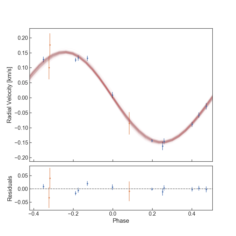
Figure 3: Phase folded radial velocity data in km s^-1 and residuals from HARPS, in blue, and FEROS, in orange, for NGTS-8. The red lines show 50 light curve models generated from randomly drawn posterior samples of the allesfitter fit.

4.2 NGTS-9

NGTS-9 was observed with the CORALIE spectrograph (Queloz et al., 2001a) on the 1.2 m Euler telescope at La Silla Observatory, Chile, between the 24th of December 2017 and the 5th of April 2018. Exposure times of either 1800  or 2700 s were used depending on seeing and general observing conditions at the time. RVs were calculated with a G2 binary mask using the standard data reduction pipelines. Initial analysis, shown phase folded in Figure 4, confirm the planetary nature of the candidate with a mass of a hot-Jupiter. The RV variations are in phase with the period detected by orion with a semi-amplitude of $K=$ $293.44\pm 15.08$ m s^-1. Correlations between RVs and bisector span and FWHM were also checked but no evidence for any such correlations was found, with a Spearman correlation of -0.05 and -0.15, respectively. The CORALIE RVs for NGTS-9 are listed in Table 5, along with their associated error, FWHM and bisector span.

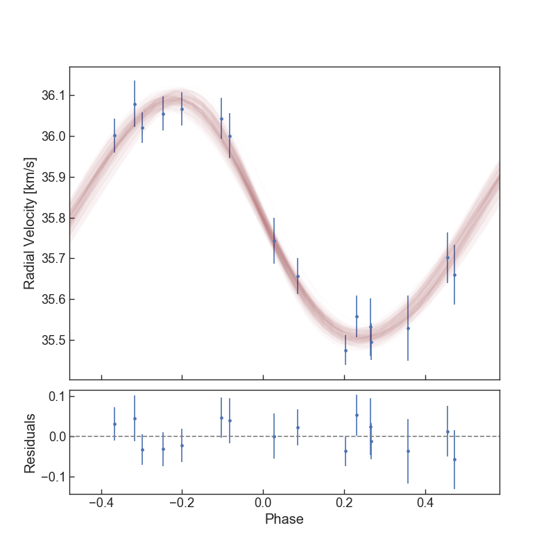
Figure 4: Phase folded radial velocity data in km s^-1 and residuals from CORALIE for NGTS-9. The red lines show 50 light curve models generated from randomly drawn posterior samples of the allesfitter fit.

Table 4: HARPS and FEROS radial velocities for NGTS-8.

JDB	RV	RV error	FWHM	BIS	Exptime	Instrument
(-2400000)	(km s-1)	(km s-1)	(km s-1)	(km s-1)	(s)
57970.7400	15.4538	0.0141	7.0583	-0.1398	1800	HARPS
57979.7893	15.7466	0.0084	6.9506	-0.0254	1800	HARPS
57980.7591	15.4692	0.0096	6.9007	-0.0021	1800	HARPS
57986.8002	15.3768	0.0147	10.4776	0.0000	1800	FEROS
57986.8147	15.4527	0.0147	10.4080	0.0360	1800	FEROS
57987.8182	15.1913	0.0108	10.5177	-0.0620	1800	FEROS
57993.6958	15.5568	0.0089	6.9108	0.0092	1800	HARPS
57994.6689	15.7472	0.0093	6.9062	-0.0238	1800	HARPS
57998.7907	15.5861	0.0109	6.9314	-0.0221	1200	HARPS
58023.6064	15.5259	0.0082	6.9028	-0.0128	1800	HARPS
58025.5985	15.4713	0.0057	6.9379	-0.0243	1800	HARPS
58026.7251	15.7423	0.0091	6.8863	-0.0141	1800	HARPS
58052.5954	15.6232	0.0107	6.9310	-0.0558	1200	HARPS
58054.6266	15.7407	0.0073	6.9014	-0.0074	1200	HARPS

Table 5: CORALIE radial velocities for NGTS-9.

JDB	RV	RV error	FWHM	BIS	Exptime	Instrument
(-2400000)	(km s-1)	(km s-1)	(km s-1)	(km s-1)	(s)
58111.8084	35.4749	0.0369	11.7616	-0.2434	2700	CORALIE
58113.7093	36.0010	0.0411	11.9519	0.0337	2700	CORALIE
58118.6806	36.0550	0.0418	12.0847	0.0198	2700	CORALIE
58129.8234	35.5313	0.0702	11.8283	0.0679	1800	CORALIE
58169.7427	35.4951	0.0448	12.0594	0.0809	2700	CORALIE
58172.5402	36.0431	0.0497	12.0437	-0.0176	2700	CORALIE
58195.5527	35.6563	0.0450	11.8628	-0.0829	2700	CORALIE
58201.7069	35.6593	0.0735	12.1195	0.0072	1800	CORALIE
58202.7184	36.0204	0.0382	11.9054	-0.0995	2700	CORALIE
58207.5924	36.0663	0.0410	11.7546	-0.0344	2700	CORALIE
58208.5990	35.7431	0.0561	11.8260	-0.0614	2700	CORALIE
58209.5025	35.5571	0.0513	12.0882	0.0690	2700	CORALIE
58210.4972	35.7017	0.0624	12.1724	0.0087	1800	CORALIE
58211.5079	36.0788	0.0566	11.8893	0.2033	1800	CORALIE
58212.5487	36.0007	0.0556	12.0946	-0.1138	1800	CORALIE
58214.4983	35.5283	0.0796	12.3596	0.1707	1800	CORALIE

5 Analysis

5.1 Stellar Properties

5.1.1 Gaia

To obtain astrometric information for NGTS-8 and NGTS-9 we crossmatched both sources with Gaia DR2. To check the quality of the astrometric solutions we calculated the unit weight error (UWE) and then renormalised UWE (RUWE). We find that both sources pass the filters recommended by the Gaia team (RUWE < 1.4, see Lindegren et al., 2018, for a discussion on the recommended UWE filters). Along with this, the two targets also have zero astrometric noise, giving us confidence that they are both single sources without evidence of unresolved binarity. They also pass the photometric filters specified by Arenou et al. (2018) to identify blended stars. With the Gaia information for each source, we calculate the absolute magnitude and plot their positions on the Hertzsprung-Russell diagram in Figure 5, where we can see that both NGTS-8 and NGTS-9 lie in the region expected for single main sequence stars.

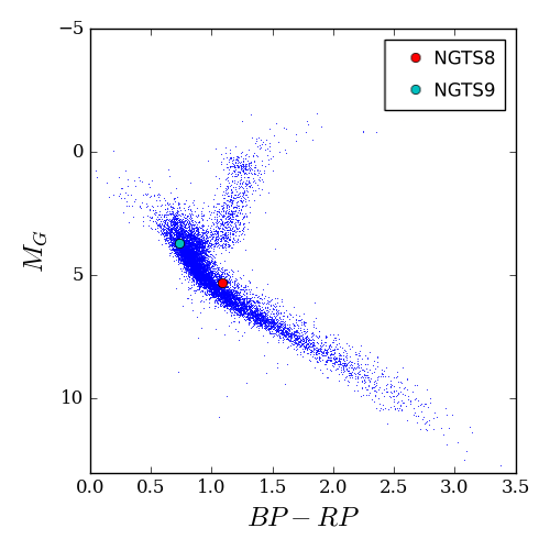
Figure 5: HR diagram using Gaia DR2 absolute magnitude. The K0V star, NGTS-8, is shown in red and the F8V, NGTS-9 in light blue.

5.1.2 SPECIES

The stacked spectra for both targets were also analyzed using SPECIES (Soto & Jenkins, 2018), a python tool to derive stellar parameters in an automated fashion from high resolution echelle spectra. By measuring the equivalent widths (EWs) for a list of irons lines, and by using the ATLAS9 model atmospheres (Castelli & Kurucz, 2004), SPECIES first solves the radiative transfer equation using MOOG (Sneden, 1973). From an iterative process, SPECIES derives then the atmospheric parameters (T_eff, log g, $[$Fe/H$]$) of our target. By interpolation through a grid of MIST isochrones (Dotter, 2016), the mass and radius are estimated, using a Bayesian approach. This method delivers an estimate of the age of the system as well. However, due to the fact that solar-type stars spend most of their lives in the evolutionary stage and because the dependence of their effective temperature and luminosity with the age of the system is weak, the estimation of the age of the system is very unconstrained for main sequence stars. Finally, SPECIES derives the rotational and macroturbulent velocities from the stellar temperature and by line-fitting to a set of five absorption lines. Parameters found by SPECIES for both targets are displayed in Table 6 and Table 7.

Table 6: Stellar Properties for NGTS-8.

Property	Value	Source
Astrometric Properties
R.A.	$21^{\mathrm{h}}55^{\mathrm{m}}54\aas@@fstack{s}2$	2MASS
Dec	$-14\degr 04\arcmin 05\aas@@fstack{\prime\prime}85$	2MASS
2MASS I.D.	$21555419$-$1404062$	2MASS
Gaia source I.D.	$6840435777723109888$	Gaia DR2
$\mu_{{\rm R.A.}}$ (mas y-1)	$21.363\pm 0.047$	Gaia DR2
$\mu_{{\rm Dec.}}$ (mas y-1)	$-10.194\pm 0.048$	Gaia DR2
parallax (mas)	$2.3027\pm 0.0299$	Gaia DR2
Photometric Properties
V (mag)	$13.68\pm 0.06$	APASS
B (mag)	$14.59\pm 0.03$	APASS
g (mag)	$14.12\pm 0.03$	APASS
r (mag)	$13.43\pm 0.06$	APASS
i (mag)	$13.21\pm 0.06$	APASS
G (mag)	$13.4954\pm 0.0003$	Gaia DR2
$\text{G}_{\text{RP}}$ (mag)	$12.8780\pm 0.0006$	Gaia DR2
$\text{G}_{\text{BP}}$ (mag)	$13.9606\pm 0.0015$	Gaia DR2
J (mag)	$12.14\pm 0.02$	2MASS
H (mag)	$11.75\pm 0.02$	2MASS
K (mag)	$11.64\pm 0.02$	2MASS
W1 (mag)	$11.59\pm 0.02$	WISE
W2 (mag)	$11.62\pm 0.02$	WISE
W3 (mag)	$11.86\pm 0.38$	WISE
Derived Properties
Spectral type	K0V	Gaia DR2
Teff (K)	$5241\pm 50$	SPECIES
$[$Fe/H$]$	$0.24\pm 0.09$	SPECIES
$v\sin i_{*}$ (km s-1)	$3.56\pm 0.67$	SPECIES
vmac (km s-1)	$1.49\pm 0.64$	SPECIES
log g	$4.41\pm 0.03$	SPECIES
Ms($M_{\odot}$)	$0.89\,^{+0.05}_{-0.04}$	SPECIES
Rs($R_{\odot}$)	$0.98\pm 0.02$	SPECIES
Age (Gyrs)	$12.48\,^{+3.23}_{-3.68}$	SPECIES
Distance (pc)	$434.273\pm 5.639$	Gaia DR2
2MASS (Skrutskie et al., 2006); APASS (Henden & Munari, 2014);
WISE (Wright et al., 2010);
Gaia DR2 (Gaia Collaboration et al., 2018)

Table 7: Stellar Properties for NGTS-9.

Property	Value	Source
Astrometric Properties
R.A.	$09^{\mathrm{h}}27^{\mathrm{m}}41\aas@@fstack{s}0$	2MASS
Dec	$-19\degr 20\arcmin 50\aas@@fstack{\prime\prime}33$	2MASS
2MASS I.D.	$09274096$-$1920515$	2MASS
Gaia source I.D.	$5678340222972504832$	Gaia DR2
$\mu_{{\rm R.A.}}$ (mas y-1)	$-6.078\pm 0.057$	Gaia DR2
$\mu_{{\rm Dec.}}$ (mas y-1)	$1.723\pm 0.063$	Gaia DR2
parallax (mas)	$1.6136\pm 0.0416$	Gaia DR2
Photometric Properties
V (mag)	$12.80\pm 0.02$	APASS
B (mag)	$13.36\pm 0.04$	APASS
g (mag)	$13.03\pm 0.05$	APASS
r (mag)	$12.65\pm 0.02$	APASS
i (mag)	$12.55\pm 0.07$	APASS
G (mag)	$12.6547\pm 0.0002$	Gaia DR2
$\text{G}_{\text{RP}}$ (mag)	$12.2157\pm 0.0013$	Gaia DR2
$\text{G}_{\text{BP}}$ (mag)	$12.9503\pm 0.0015$	Gaia DR2
J (mag)	$11.71\pm 0.03$	2MASS
H (mag)	$11.49\pm 0.02$	2MASS
K (mag)	$11.45\pm 0.02$	2MASS
W1 (mag)	$11.39\pm 0.02$	WISE
W2 (mag)	$11.42\pm 0.02$	WISE
W3 (mag)	$11.58\pm 0.20$	WISE
Derived Properties
Spectral type	F8V	Gaia DR2
Teff (K)	$6330\pm 130$	SPECIES
$[$Fe/H$]$	$0.31\pm 0.15$	SPECIES
$v\sin i_{*}$ (km s-1)	$6.38\pm 1.05$	SPECIES
vmac (km s-1)	$5.47\pm 1.05$	SPECIES
log g	$4.37\pm 0.20$	SPECIES
Ms($M_{\odot}$)	$1.34\pm 0.05$	SPECIES
Rs($R_{\odot}$)	$1.38\pm 0.04$	SPECIES
Age (Gyrs)	$0.96\pm 0.60$	SPECIES
Distance (pc)	$619.732\pm 15.977$	Gaia DR2
2MASS (Skrutskie et al., 2006); APASS (Henden & Munari, 2014);
WISE (Wright et al., 2010);
Gaia DR2 (Gaia Collaboration et al., 2018)

5.2 Stellar Activity and Rotation on NGTS-8

In addition to modeling the stellar parameters, we also attempted to search for stellar activity and rotation signals. As mentioned earlier, the out-of-eclipse light curves of both targets show no appreciable variability, and there are no correlations with the measured RVs and the bisector or the FWHM for the two targets – see Section 4. Nonetheless, determining the stellar rotation period, along with knowledge of the stellar radius and $v\sin i_{*}$, can enable the inclination angle of the stellar rotation axis to be constrained. This can enable misaligned star-planet systems to be identified (Watson et al., 2010).

In order to put constraints on the stellar rotation period, two methods were used. The first one consists of using the activity of the star. Using the formulae described in Lovis et al. (2011), the $\log R^{\prime}_{HK}$ was measured for each individual HARPS spectrum. Since the $\log R^{\prime}_{HK}$ of NGTS-9, an F8V star, was not measurable, we will only focus on the K0V star, NGTS-8, in this section. The calculated value of the $\log R^{\prime}_{HK}$ varied between $-4.643$ and $-5.053$ in the individual spectra due to a low signal-to-noise ratio in the blue band, with a mean value of $-4.783$. In order to increase the precision of the measured data, a stacked spectrum of all the spectra was created. Figure 6 shows this spectrum, zoomed on the H (3933.664 Å) and K (3968.470 Å) bands, represented with dashed lines. Using this spectrum, we found a value of $-4.817\pm 0.110$ for the $\log R^{\prime}_{HK}$. Finally, using the relation from Noyes et al. (1984), the stellar rotation period of NGTS-8 was derived to be $37.7\pm 4.1$ days.

Our second approach used the $v\sin i_{*}$ of the star measured from SPECIES and assumed that the stellar inclination angle, $i_{*}$, was 90^∘ (i.e. $\sin(i_{*})=1$). This then enables an upper limit to be placed on the stellar rotation period when the stellar radius is known (e.g. Watson et al. 2010). An upper limit of $13.92\pm 2.64$ days was found, which is discrepant with our previous result by almost 5 sigma and would rule out the long rotation period inferred from the $\log R^{\prime}_{HK}$ measurement. Even adopting the most extreme individual $\log R^{\prime}_{HK}$ measurement implies a stellar rotation period greater than 26 days.

Given this discrepancy, we decided to verify the $v\sin i_{*}$ value measured by SPECIES with another technique. We did this by taking a stellar spectrum of a slowly rotating star of the same spectral type as NGTS-8  and artificially broadening it by different $v\sin i_{*}$ amounts (using a Gray rotational broadening profile). The projected rotational broadening of NGTS-8  was then measured using an optimal-subtraction technique in which the broadened template spectra were multiplied by a constant and then subtracted from the NGTS-8  spectrum. This is done after correcting for radial velocity shifts and re-interpolating to a constant velocity scale. The value of the rotational broadening is then the one that minimises the scatter in the residual spectrum after performing the optimal subtraction. For our template spectrum, we used $\alpha$ Cen B, which has a spectral type very close to NGTS-8  and a low rotation rate. We constructed the template spectrum by stacking archival HARPS spectra taken over 1 night when $\alpha$ Cen B was known to be inactive. The result of this analysis yielded a value consistent with that found by SPECIES.

Adopting the firm upper-limit on the stellar rotation period from the $v\sin i_{*}$ measurement would ordinarily lead to a much higher $\log R^{\prime}_{HK}$ level than the one observed. While no definitive answer can explain this difference, some systems hosting hot-Jupiters are known to have suppressed Ca II H & K re-emission (e.g. WASP-12 – Fossati et al. 2013), leading to a lower measured value of the $\log R^{\prime}_{HK}$. However, these systems generally contain hot-Jupiters very close to filling their Roche lobes, which is not the case for our planet, NGTS-8b. We therefore conclude that the most likely explanation of the discrepancy is that we have caught NGTS-8 in an extended low-activity state.

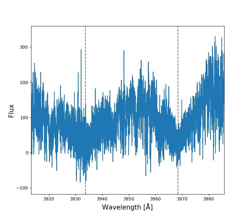
Figure 6: Stacked spectrum of NGTS-8 from HARPS, zoomed on the H (3933.664 Å) and K (3968.470 Å) bands, represented with dashed lines.

5.3 Global Modelling

Analysis of the different photometric and spectroscopic data was performed on NGTS-8 and NGTS-9 data using allesfitter (Günther & Daylan, 2019, and in prep.). allesfitter is a user-friendly and publicly available software package for modeling data from photometric and RV instruments. Its generative model can account for multi-star systems, stellar flares, star spots and multiple exoplanets. For this, it constructs an inference framework that unites the versatile packages ellc (light curve and RV models; Maxted, 2016), aflare (flare model; Davenport et al., 2014), dynesty (nested samplingl; Speagle, 2019), emcee (MCMC sampling; Foreman-Mackey et al., 2013), and celerite (GP models; Foreman-Mackey et al., 2017). allesfitter is accesible at https://github.com/MNGuenther/allesfitter.

For NGTS-8 and NGTS-9, the Nested Sampling approach (see Skilling 2004) was used, which enables simultaneous fitting of the transit light curves and radial velocity data. In particular, we fit for the following astrophysical parameters: a planet’s orbital period $P$, the transit epoch $T_{C}$, the radius ratio $R_{p}/R_{\star}$, the sum of radii over the semi-major axis $(R_{p}+R_{\star})/a$, the cosine of the inclination $\cos{i}$, the eccentricity and argument of periastron parameterized as $\sqrt{e}\sin{\omega}$ and $\sqrt{e}\cos{\omega}$, and the RV semi-amplitude $K$. For the transit light curve modeling, a quadratic limb-darkening law was adopted parameterized after Kipping (2013) as $u_{1}$ and $u_{2}$. Systematic trends in the transit light curves were modeled by a Gaussian process with Matern 3/2 kernels parameterized by the GP’s amplitude $\ln{\rho}$ and time scale $\ln{\sigma}$. For both planets, all photometric data were used for the fits as well as all spectroscopic data, with instrumental offsets taken into account, relevant for NGTS-8  where HARPS and FEROS data were combined for the modelling.

We find that NGTS-8b has a mass of $0.93\,^{+0.04}_{-0.03}$ M_J and a radius $1.09\pm 0.03$ R_J, while NGTS-9b has a mass of $2.90\pm 0.17$ M_J and a radius $1.07\pm 0.06$ R_J. The results of the fits for the two planets are summarized in Tables 8 and 9 and shown in earlier plots. Figure 1 shows (in red) 20 light curve models generated from randomly drawn posterior samples of the allesfitter fit to the NGTS, SAAO and Euler light curves, respectively, for NGTS-8. In the same way, Figure 2 shows the photometric data of NGTS, SAAO and Euler, respectively, for NGTS-9, with (in red) 20 light curve models generated from randomly drawn posterior samples of the allesfitter fit. For the RV data, Figure 3 shows the modelling of HARPS, blue points, and FEROS, orange points, for NGTS-8 and Figure 4 shows the modelling of the CORALIE data for NGTS-9.

In order to check our results, we also performed another analysis of the photometric data from NGTS and available spectroscopic data on NGTS-8 and NGTS-9 using the EXOplanet traNsits and rAdIal veLocity fittER (EXO-NAILER – Espinoza et al. 2016). Using the Markov chain Monte Carlo (MCMC) with a total of 250 walkers for 20000 jumps and 5000 burn-in steps, the modelling was done assuming pure white-noise for the inputted light curves. A logarithmic limb-darkening law was adopted with limb-darkening coefficients taken from Claret et al. (2013), and sampled according to Espinoza & Jordán (2015). The results from this second analysis all agreed, within the error bars, with those found from allesfitter.

5.4 TESS

During the preparation of this manuscript TESS photometry was released for NGTS-9, which was observed in Sector 8. In response to this data release, we re-analysed, using all available data, NGTS-9 with allesfitter. The TESS photometric data is presented in Figure 7 with the models generated from the fit. We confirmed that using TESS data in our modelling of NGTS-9 did not change or improve the values obtained, and thus the TESS data was not taken into account in the analysis presented in this work. The fact that TESS does not improve the results can be explained by the magnitude of NGTS-9, $V=12.80\pm 0.02$. At these magnitudes we have found that NGTS and TESS perform similarly (Wheatley et al., 2018). No TESS data is available for NGTS-8.

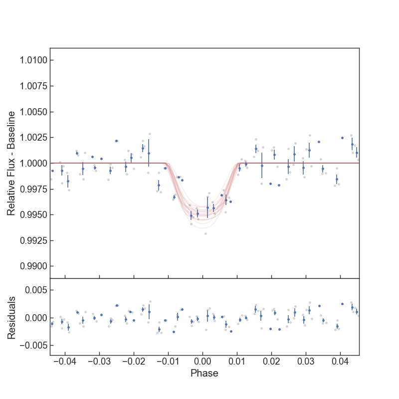
Figure 7: TESS light curve of NGTS-9b with residuals. The blue data points are binned every 7 min to aid visualisation. The red lines show 20 light curve models generated from randomly drawn posterior samples of the allesfitter fit.

Table 8: Planetary properties for NGTS-8b using allesfitter.

Property	Value
P (days)	$2.49970\pm 0.00001$
TC (BJD)	$2457500.17830\pm 0.00072$
T14 (hours)	$2.61\pm 0.06$
$a/R_{*}$	$7.60\pm 0.18$
$R/R_{*}$	$0.114\pm 0.002$
K (m s-1)	$149.95\pm 3.56$
e	$0.010\,^{+0.014}_{-0.010}$
i (degrees)	$86.9\pm 0.5$
Mp(MJ)	$0.93\,^{+0.04}_{-0.03}$
Rp(RJ)	$1.09\pm 0.03$
$\rho_{p}$ (g cm-3)	$0.89\,^{+0.08}_{-0.07}$
a (AU)	$0.035\pm 0.001$
Teq (K)	$1345\pm 19$

Table 9: Planetary properties for NGTS-9b using allesfitter.

Property	Value
P (days)	$4.43527\pm 0.00002$
TC (BJD)	$2457671.81086\pm 0.00265$
T14 (hours)	$2.05\pm 0.07$
$a/R_{*}$	$9.06\pm 0.31$
$R/R_{*}$	$0.080\pm 0.004$
K (m s-1)	$293.44\pm 15.08$
e	$0.060^{+0.076}_{-0.052}$
i (degrees)	$84.1\pm 0.4$
Mp(MJ)	$2.90\pm 0.17$
Rp(RJ)	$1.07\pm 0.06$
$\rho_{p}$ (g cm-3)	$2.93^{+0.53}_{-0.49}$
a (AU)	$0.058^{+0.003}_{-0.002}$
Teq (K)	$1448\pm 36$

6 Discussion

As outlined in the introduction, at incident fluxes greater than $2\times 10^{5}$ W m^-2 (Miller & Fortney 2011; Demory & Seager 2011), hot-Jupiters are increasingly found with radii that are significantly larger than theoretically predicted (Anderson et al. 2011; Delrez et al. 2016; Almenara et al. 2015). Using Gaia DR2 measurements for the stellar luminosity and the orbital parameters listed in Tables 6 and 8 for NGTS-8b and listed in Tables 7 and 9 for NGTS-9b, we calculated the flux received by both planets to be greater than this limit ($6.85\pm 0.45\times 10^{5}$ W m^-2 and $9.92\pm 1.09\times 10^{5}$ W m^-2 for NGTS-8b and NGTS-9b, respectively). Thus, the stellar irradiation levels received by both of these planets puts them firmly in the regime where we might expect them to exhibit larger than predicted planetary radii.

Sestovic et al. (2018) conducted a statistical investigation on hot-Jupiter radii and found that above a threshold in incident flux ($2\times 10^{5}$ W m^-2 Miller & Fortney 2011; Demory & Seager 2011), the observed radius follow the thermal evolution models (Miller & Fortney 2011; Thorngren et al. 2016) with the addition of an inflation parameter, $\Delta R$. This observed radius ‘inflation’ is dependent on both the incident stellar flux and the mass of the planet. They proposed a flux-mass-radius relationship that has distinct forms for 4 different planetary mass regimes: below 0.37 M_J, between 0.37 – 0.98 M_J, between 0.98 – 2.50 M_J and over 2.50 M_J. Using these relationships, we calculated what would be the expected radius inflation ($\Delta R$) values for our two planets. For NGTS-8b, its mass lies on the edge of two regimes in Sestovic et al. (2018) (M_p < 0.98 M_J and M_p > 0.98 M_J), we thus determined predicted $\Delta R$s from both relationships of $0.24\pm 0.02$ and $0.02\pm 0.01$ R_J, respectively. While the first value would suggest a highly inflated radius, the second value however suggests almost no inflation. Concerning NGTS-9b, the predicted radius inflation, $\Delta R$, is $0.18\pm 0.01$ R_J. Thus, from the work of Sestovic et al. (2018), these two planets would be expected to exhibit planetary radii larger than predicted.

Table 10: A summary of the mass-radius model for NGTS-8b with radius $1.09\pm 0.03$ R_J.

Model	Mass of the	Orbital	Age of the	Mass fraction of	Core	Radius
	planet (MJ)	separation (AU)	system (Gyrs)	heavy material	mass (%)	(RJ)
Baraffe et al. (2008)	1	0.045	8.93 - 10.00	0.02 - 0.1		1.025 - 1.074
Fortney et al. (2007)	1	0.045	4.5		0 - 25	1.050 - 1.107

Table 11: A summary of the mass-radius model for NGTS-9b with radius $1.07\pm 0.06$ R_J.

Model	Mass of the	Orbital	Age of the	Mass fraction of	Core	Radius
	planet (MJ)	separation (AU)	system (Gyrs)	heavy material	mass (%)	(RJ)
Baraffe et al. (2008)	2 - 5	0.045	0.30 - 1.78	0.02 - 0.1		1.063 - 1.177
Fortney et al. (2007)	2.44	0.045	0.30 - 1		0 - 100	1.065 - 1.199

We finally compared the observed planetary radii of NGTS-8b and NGTS-9b to the mass-radius models of Baraffe et al. (2008) and Fortney et al. (2007) who present, assuming a solar-type star, tables of planetary radii as a function of core mass, mass of the planet, orbital separation and age of the system. Since neither of the host stars of the planets presented here are solar-like, we had to renormalise the orbital separation in order to keep the same incident flux. In this scenario, the distance from their host star would be equal to $0.044$ AU and $0.038$ AU for NGTS-8b and NGTS-9b, respectively. As one can see in Tables 10 and 11, both models seem consistent and correctly predict the measured radius of NGTS-8b, $1.09\pm 0.03$ R_J, and NGTS-9b, $1.07\pm 0.06$ R_J, using the described parameters.

To conclude, even if both planets are in a regime where we expect planets to exhibit larger than predicted radii, our two planets are non-inflated hot-Jupiters. This could be due to the planets being enriched with heavy elements, yielding a more compact structure and thus a smaller radius, like HD 149026b (Sato et al., 2005).

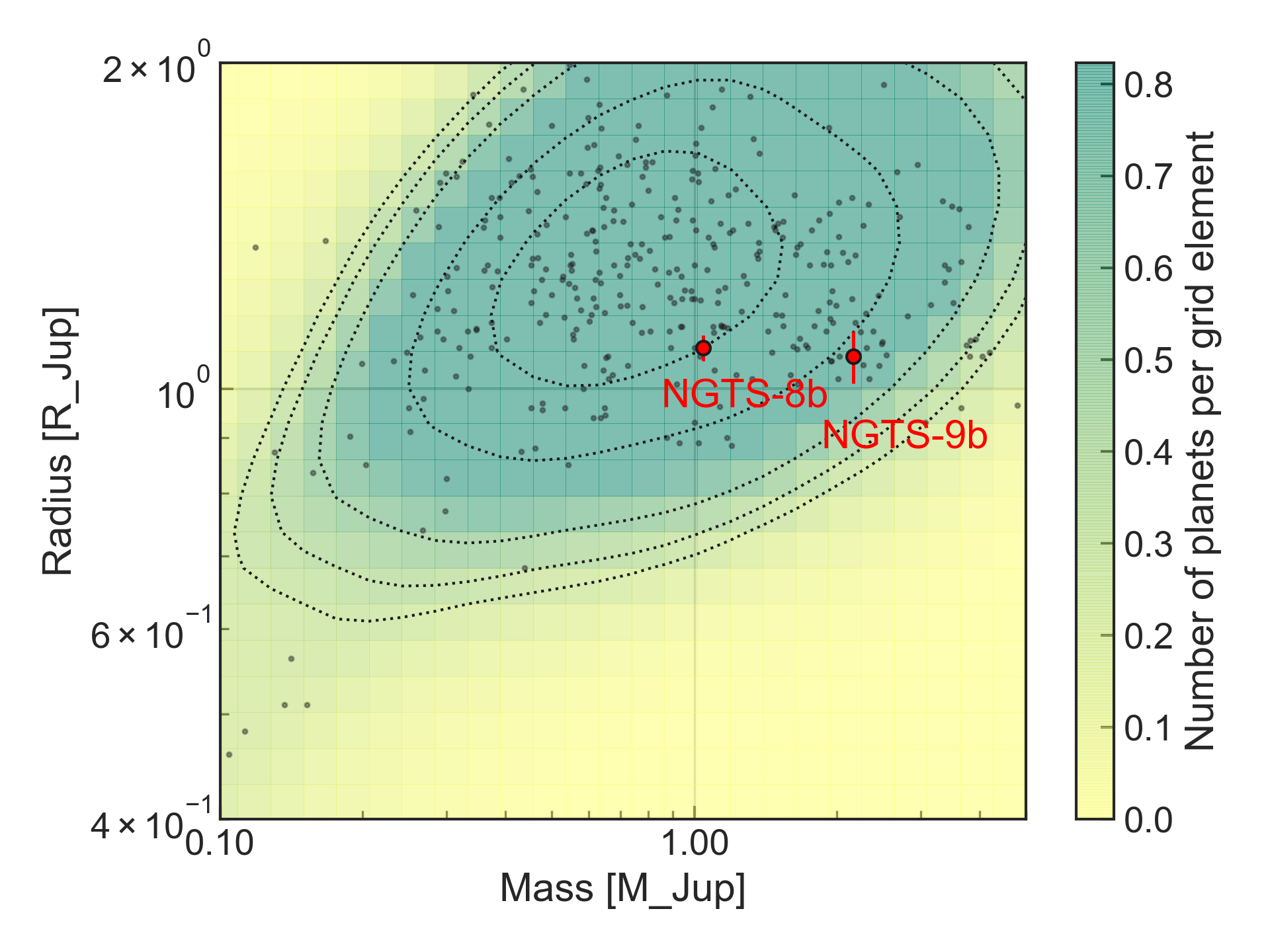
Figure 8: Shows NGTS-8b and NGTS-9b in the planetary radius vs planetary mass plot, in regards with all exoplanets from the NASA Exoplanet Archive with radius uncertainty below 10% or mass uncertainty below 50% and with an incident flux received by the planets greater than $2\times 10^{5}$ W m^-2. The background and the dotted black lines represents the point density per grid element.

7 Conclusions

We have presented the latest discovery by the Next Generation Transit Survey (NGTS) of two non-inflated hot-Jupiters: NGTS-8b and NGTS-9b. NGTS, SAAO and Euler photometric data and spectroscopic data from HARPS, FEROS and CORALIE were used to confirm the detection of these two planets. By combining some of these data, an analysis of the transiting planets was performed using allesfitter and confirmed with EXO-NAILER. From this model, both planets have orbits consistent with being circular, as expected for such short period hot-Jupiters. The characteristic of the planets were calculated such as: NGTS-8b with a mass of $0.93\,^{+0.04}_{-0.03}$ M_J and a radius $1.09\pm 0.03$ R_J, and NGTS-9b with a mass of $2.90\pm 0.17$ M_J and a radius of $1.07\pm 0.06$ R_J. Figure 8 shows these discoveries in comparison to known planets with radius higher than 0.4 R_J.

A study of the rotational period of the K0V star, NGTS-8, was performed using different models and despite a significant discrepancy that we assume is due to an extended low activity of the star, we measured an upper limit of $13.92\pm 2.64$ days. While its host is considerably fainter, our analysis also suggests that its planet, NGTS-8b, could have similar properties to HD 189733b, one of the best studied hot-Jupiters. Further observations of NGTS-8b will allow direct comparisons to be drawn between these two hot-Jupiters. The upcoming launch of JWST will enable high-precision observations of NGTS-8b’s full-phase curve, which would be of particular interest due to the efficient dayside to nightside heat recirculation that HD 189733b exhibits relative to other hot-Jupiters (Knutson et al. 2007; Schwartz et al. 2017).

Concerning NGTS-9b, the planet is highly irradiated, with an incident flux around $9.59\pm 0.74\times 10^{5}$ W m^-2, yet non-inflated. This radius could be due to the planet being extremely enriched with heavy elements, explaining its density, $2.93^{+0.53}_{-0.49}$ g cm^-3, one of the highest compare to planets with similar masses, as shown in Figure 8.

References

- Almenara et al. (2015) Almenara J., et al., 2015, Astronomy & Astrophysics, 575, A71
- Anderson et al. (2011) Anderson D., et al., 2011, Monthly Notices of the Royal Astronomical Society, 416, 2108
- Arenou et al. (2018) Arenou F., et al., 2018, A&A, 616, A17
- Arras & Socrates (2010) Arras P., Socrates A., 2010, The Astrophysical Journal, 714, 1
- Baraffe et al. (2008) Baraffe I., Chabrier G., Barman T., 2008, A&A, 482, 315
- Barbary (2016) Barbary K., 2016, SEP: Source Extractor as a library, The Journal of Open Source Software, doi:10.21105/joss.00058
- Batygin & Stevenson (2010) Batygin K., Stevenson D. J., 2010, The Astrophysical Journal Letters, 714, L238
- Bayliss et al. (2018) Bayliss D., et al., 2018, MNRAS, 475, 4467
- Bodenheimer et al. (2001) Bodenheimer P., Lin D., Mardling R., 2001, The Astrophysical Journal, 548, 466
- Bodenheimer et al. (2003) Bodenheimer P., Laughlin G., Lin D. N., 2003, The Astrophysical Journal, 592, 555
- Brahm et al. (2017) Brahm R., Jordán A., Espinoza N., 2017, Publications of the Astronomical Society of the Pacific, 129, 034002
- Burrows et al. (2007) Burrows A., Hubeny I., Budaj J., Hubbard W., 2007, The Astrophysical Journal, 661, 502
- Castelli & Kurucz (2004) Castelli F., Kurucz R. L., 2004, ArXiv Astrophysics e-prints,
- Chabrier & Baraffe (2007) Chabrier G., Baraffe I., 2007, The Astrophysical Journal Letters, 661, L81
- Claret et al. (2013) Claret A., Hauschildt P. H., Witte S., 2013, A&A, 552, A16
- Collier Cameron et al. (2006) Collier Cameron A., et al., 2006, MNRAS, 373, 799
- Coppejans et al. (2013) Coppejans R., et al., 2013, Publications of the Astronomical Society of the Pacific, 125, 976
- Craig et al. (2015) Craig M. W., et al., 2015, ccdproc: CCD data reduction software, Astrophysics Source Code Library (ascl:1510.007)
- Davenport et al. (2014) Davenport J. R. A., et al., 2014, ApJ, 797, 122
- Delrez et al. (2016) Delrez L., et al., 2016, Monthly Notices of the Royal Astronomical Society, 458, 4025
- Demory & Seager (2011) Demory B.-O., Seager S., 2011, ApJS, 197, 12
- Dotter (2016) Dotter A., 2016, ApJS, 222, 8
- Espinoza & Jordán (2015) Espinoza N., Jordán A., 2015, MNRAS, 450, 1879
- Espinoza et al. (2016) Espinoza N., et al., 2016, The Astrophysical Journal, 830, 43
- Foreman-Mackey et al. (2013) Foreman-Mackey D., Hogg D. W., Lang D., Goodman J., 2013, PASP, 125, 306
- Foreman-Mackey et al. (2017) Foreman-Mackey D., Agol E., Ambikasaran S., Angus R., 2017, celerite: Scalable 1D Gaussian Processes in C++, Python, and Julia, Astrophysics Source Code Library (ascl:1709.008)
- Fortney et al. (2007) Fortney J. J., Marley M. S., Barnes J. W., 2007, The Astrophysical Journal, 659, 1661
- Fossati et al. (2013) Fossati L., Ayres T. R., Haswell C. A., Bohlender D., Kochukhov O., Flöer L., 2013, ApJ, 766, L20
- Gaia Collaboration et al. (2018) Gaia Collaboration Brown A. G. A., Vallenari A., Prusti T., de Bruijne J. H. J., Babusiaux C., Bailer-Jones C. A. L., 2018, preprint, (arXiv:1804.09365)
- Ginzburg & Sari (2016) Ginzburg S., Sari R., 2016, The Astrophysical Journal, 819, 116
- Guillot & Showman (2002) Guillot T., Showman A. P., 2002, Astronomy & Astrophysics, 385, 156
- Günther & Daylan (2019) Günther M. N., Daylan T., 2019, allesfitter: Flexible star and exoplanet inference from photometry and radial velocity (ascl:1903.003)
- Günther et al. (2018) Günther M. N., et al., 2018, MNRAS, 478, 4720
- Henden & Munari (2014) Henden A., Munari U., 2014, Contributions of the Astronomical Observatory Skalnate Pleso, 43, 518
- Jermyn et al. (2017) Jermyn A. S., Tout C. A., Ogilvie G. I., 2017, Monthly Notices of the Royal Astronomical Society, 469, 1768
- Kaufer & Pasquini (1998) Kaufer A., Pasquini L., 1998, in D’Odorico S., ed., Proc. SPIEVol. 3355, Optical Astronomical Instrumentation. pp 844–854, doi:10.1117/12.316798
- Kipping (2013) Kipping D. M., 2013, MNRAS, 435, 2152
- Knutson et al. (2007) Knutson H. A., et al., 2007, Nature, 447, 183
- Lendl et al. (2012) Lendl M., et al., 2012, A&A, 544, A72
- Lindegren et al. (2018) Lindegren L., et al., 2018, A&A, 616, A2
- Lovis et al. (2011) Lovis C., et al., 2011, arXiv e-prints, p. arXiv:1107.5325
- Maxted (2016) Maxted P. F. L., 2016, A&A, 591, A111
- Mayor et al. (2003) Mayor M., et al., 2003, The Messenger, 114, 20
- McCormac et al. (2013) McCormac J., Pollacco D., Skillen I., Faedi F., Todd I., Watson C. A., 2013, PASP, 125, 548
- Miller & Fortney (2011) Miller N., Fortney J. J., 2011, The Astrophysical Journal Letters, 736, L29
- Noyes et al. (1984) Noyes R. W., Hartmann L. W., Baliunas S. L., Duncan D. K., Vaughan A. H., 1984, ApJ, 279, 763
- Perna et al. (2010) Perna R., Menou K., Rauscher E., 2010, The Astrophysical Journal, 724, 313
- Queloz et al. (2001a) Queloz D., et al., 2001a, The Messenger, 105, 1
- Queloz et al. (2001b) Queloz D., et al., 2001b, A&A, 379, 279
- Raynard et al. (2018) Raynard L., et al., 2018, MNRAS, 481, 4960
- Sato et al. (2005) Sato B., et al., 2005, The Astrophysical Journal, 633, 465
- Schwartz et al. (2017) Schwartz J. C., Kashner Z., Jovmir D., Cowan N. B., 2017, ApJ, 850, 154
- Sestovic et al. (2018) Sestovic M., Demory B.-O., Queloz D., 2018, A&A, 616, A76
- Skilling (2004) Skilling J., 2004, in AIP Conference Proceedings. pp 395–405
- Skrutskie et al. (2006) Skrutskie M. F., et al., 2006, AJ, 131, 1163
- Sneden (1973) Sneden C. A., 1973, PhD thesis, THE UNIVERSITY OF TEXAS AT AUSTIN.
- Soto & Jenkins (2018) Soto M. G., Jenkins J. S., 2018, A&A, 615, A76
- Speagle (2019) Speagle J. S., 2019, arXiv e-prints, p. 1904.02180
- Tamuz et al. (2005) Tamuz O., Mazeh T., Zucker S., 2005, MNRAS, 356, 1466
- Thorngren et al. (2016) Thorngren D. P., Fortney J. J., Murray-Clay R. A., Lopez E. D., 2016, ApJ, 831, 64
- Tremblin et al. (2017) Tremblin P., et al., 2017, The Astrophysical Journal, 841, 30
- Vines et al. (2019) Vines J. I., et al., 2019, arXiv e-prints, p. arXiv:1904.07997
- Watson et al. (2010) Watson C., Littlefair S., Cameron A. C., Dhillon V., Simpson E., 2010, Monthly Notices of the Royal Astronomical Society, 408, 1606
- West et al. (2018) West R. G., et al., 2018, arXiv e-prints, p. arXiv:1809.00678
- Wheatley et al. (2018) Wheatley P. J., et al., 2018, MNRAS, 475, 4476
- Wright et al. (2010) Wright E. L., et al., 2010, AJ, 140, 1868
- Wu & Lithwick (2012) Wu Y., Lithwick Y., 2012, The Astrophysical Journal, 763, 13
- Youdin & Mitchell (2010) Youdin A. N., Mitchell J. L., 2010, The Astrophysical Journal, 721, 1113