Estimating the molecular gas mass of low-redshift galaxies from a combination of mid-infrared luminosity and optical properties

Abstract

We present CO(J=1-0) and/or CO(J=2-1) spectroscopy for 31 galaxies selected from the ongoing Mapping Nearby Galaxies at Apache Point Observatory (MaNGA) survey, obtained with multiple telescopes. This sample is combined with CO observations from the literature to study the correlation of the CO luminosities ($L_{\rm CO(1-0)}$) with the mid-infrared luminosities at 12 ($L_{\mbox{12\micron}}$) and 22 µm ($L_{\mbox{22\micron}}$), as well as the dependence of the residuals on a variety of galaxy properties. The correlation with $L_{\mbox{12\micron}}$ is tighter and more linear, but galaxies with relatively low stellar masses ($M_{\ast}\lesssim 10^{10}$ M_⊙) and blue colors ($g-r\lesssim 0.5$ and/or NUV$-r$ $\lesssim 3$) fall significantly below the mean $L_{\rm CO(1-0)}$–$L_{\mbox{12\micron}}$ relation. We propose a new estimator of the CO(1-0) luminosity (and thus the total molecular gas mass $M_{\rm mol}$) that is a linear combination of three parameters: $L_{\mbox{12\micron}}$, $M_{\ast}$ and $g-r$. We show that, with a scatter of only 0.18 dex in log $(L_{\rm CO(1-0)})$, this estimator provides unbiased estimates for galaxies of different properties and types. An immediate application of this estimator to a compiled sample of galaxies with only CO(J=2-1) observations yields a distribution of the CO(J=2-1) to CO(J=1-0) luminosity ratios ($R21$) that agrees well with the distribution of real observations, in terms of both the median and the shape. Application of our estimator to the current MaNGA sample reveals a gas-poor population of galaxies that are predominantly early-type and show no correlation between molecular gas-to-stellar mass ratio and star formation rate, in contrast to gas-rich galaxies. We also provide alternative estimators with similar scatters, based on $r$ and/or $z$ band luminosities instead of $M_{\ast}$. These estimators serve as cheap and convenient $M_{\rm mol}$ proxies to be potentially applied to large samples of galaxies, thus allowing statistical studies of gas-related processes of galaxies.

1 Introduction

In current galaxy formation models, galaxies form at the centers of dark matter haloes, where gas is able to cool, condense and form stars (e.g. White & Rees, 1978). It is thus crucial to understand the physical processes that regulate gas accretion and cycling in/around galaxies before one can have a complete picture of galaxy formation and evolution. Despite of a rich history of studies, however, our understanding of the cold gas content of galaxies has been rather limited due to the lack of large surveys at radio/mm/sub-mm wavelengths. Large surveys aiming to detect Hi in nearby galaxies have become available only in recent years, such as the Hi Parkes All-Sky Survey (HIPASS; Zwaan et al., 2005) and the Arecibo Legacy Fast ALFA (ALFALFA) survey (Giovanelli et al., 2005). For molecular gas content, there have also been recent efforts of establishing uniform samples of CO detections for nearby galaxies, such as the CO Legacy Data base for the GASS (COLD GASS; Saintonge et al., 2011) and the extended COLD GASS (xCOLD GASS; Saintonge et al., 2017) surveys. Unfortunately, when compared to optical surveys, these surveys are still relatively shallow and small, limited to low redshifts (mostly $z<0.2$) and with poor spatial resolution.

In order for statistical studies of both the stellar and gaseous content of galaxies, there have been many attempts to estimate the cold gas content (both Hi and H₂ mass) for large samples of optically-detected galaxies, using galaxy properties that can be more easily obtained. The current Hi surveys, together with compiled catalogs of Hi detections from the literature (e.g. HyperLeda; Paturel et al., 2003), have revealed that the Hi gas-to-stellar mass ratio ($M_{\rm HI}/M_{\ast}$) correlates with a variety of galaxy properties, including specific star formation rate (sSFR) and related parameters such as optical, optical–near-infrared (NIR) and near-ultraviolet (NUV)–optical colors (e.g. Kannappan, 2004; Zhang et al., 2009; Catinella et al., 2010), as well as structural parameters such as stellar light or mass surface density (e.g. Zhang et al., 2009; Li et al., 2012). Such scaling relations have motivated many attempts to calibrate colors, H$\alpha$ luminosity, or a combination of multiple parameters as proxies for $M_{\rm HI}/M_{\ast}$, providing estimated Hi masses for large samples of galaxies, thus allowing statistical studies of gas-related processes (e.g. Kannappan, 2004; Tremonti et al., 2004; Erb et al., 2006; Zhang et al., 2009; Catinella et al., 2010; Li et al., 2012; Brinchmann et al., 2013; Kannappan et al., 2013; Zhang et al., 2013; Eckert et al., 2015; Rafieferantsoa et al., 2018; Zu, 2018). Such estimators typically have a scatter of $\sim 0.25-0.4$ dex in log$(M_{\rm HI}/M_{\ast})$.

As pointed out in Zhang et al. (2009, see their Section 3.2), such Hi gas mass estimators can be understood from the Kennicutt-Schmidt (KS) star formation relation (Schmidt, 1959; Kennicutt, 1998), that relates the star formation rate per unit area ($\Sigma_{\rm SFR}$) to the surface mass density of cold gas ($\Sigma_{\rm gas}$) in a galactic disc. Because star formation is expected to occur in cold giant molecular clouds (Solomon et al., 1987; McKee & Ostriker, 2007; Bolatto et al., 2008), one might expect the CO (and H₂) emission to present tighter correlations with SFR-related properties than the Hi emission. Indeed, the KS law with molecular gas surface densities measured from CO emission is found to be more linear (with a slope closer to unity) than that from Hi emission (e.g. Bigiel et al., 2008; Leroy et al., 2008). Meanwhile, Gao & Solomon (2004) find a tight linear relation between the integrated SFRs and dense molecular gas masses (derived from HCN emission) of normal and starburst galaxies. Combined with some CO observations at high redshifts (e.g. Carilli & Walter, 2013; Riechers et al., 2019), previous studies have also shown that the molecular gas content of galaxies is well correlated with the cosmic star formation rate density (e.g. Kruijssen, 2014; Saintonge et al., 2017; Tacconi et al., 2018). In addition, the ratio of H₂ mass (inferred from CO emission observations) to stellar mass ($M_{\rm H_{2}}/M_{\ast}$) is found to correlate with sSFR and NUV$-r$ of nearby galaxies, as nicely shown by the COLD GASS (Saintonge et al., 2011) and xCOLD GASS (Saintonge et al., 2017) surveys. However, in the same surveys, $M_{\rm H_{2}}/M_{\ast}$ shows only a mild dependence on stellar mass at $M_{\ast}<10^{10.5}$ M_⊙ and on stellar surface mass density at $\mu_{\ast}\lesssim 10^{8.7}$ M_⊙ kpc^-2, before it drops sharply at higher masses and/or surface densities. This behavior is in contrast to $M_{\rm HI}/M_{\ast}$, that decreases quasi-linearly with increasing $M_{\ast}$ or $\mu_{\ast}$ down to $M_{\rm HI}/M_{\ast}\sim 0.01$ at log$(\mu_{\ast}$/ (M_⊙ kpc^-2)) $\sim 9.6$ (e.g. Zhang et al., 2009, see their Fig. 2).

Apparently, the molecular gas content of galaxies doesn’t scale with their optical properties in a simple way. Many studies have attempted to link the molecular gas content of galaxies with their infrared luminosities. For instance, far-infrared (FIR) or sub-mm continuum observations are commonly used to derive total dust masses, from which total gas masses are inferred with the (metallicity-dependent) gas-to-dust mass ratio (e.g. Israel, 1997; Leroy et al., 2011; Magdis et al., 2011; Eales et al., 2012; Sandstrom et al., 2013; Scoville et al., 2014; Groves et al., 2015). This gas-to-dust ratio is relatively constant, considering the extremely large CO-to-H2 conversion factor in extremely metal-poor galaxies (Shi et al., 2016). A new survey, JINGLE (JCMT dust and gas In Nearby Galaxies Legacy Exploration), is obtaining both integrated CO line spectroscopy and 850 µm continuum fluxes for nearby galaxies using the 15-m James Clark Maxwell Telescope (JCMT). It will study the scaling relations of cold gas and dust masses with global galaxy properties such as stellar mass, SFR and gas-phase metallicity (Saintonge et al., 2018).

Furthermore, thanks to the Wide-field Infrared Survey Explorer (WISE; Wright et al., 2010), mid-infrared (MIR) luminosities have recently been found to strongly correlate with CO emission in both nearby star-forming late-type and (generally non-star-forming) early-type galaxies (Kokusho et al., 2017, 2019). Some authors found WISE 4.6-12 µm color to strongly correlate with star formation activity (Donoso et al., 2012) and molecular gas mass fraction (Yesuf et al., 2017). By jointly analyzing the WISE data and the CO observations from COLD GASS, Analysis of the interstellar Medium of Isolated GAlaxies (AMIGA; Lisenfeld et al., 2011) and their own sample observed with Sub-millimeter Telescope (SMT), Jiang et al. (2015) found both the CO(J=1-0) and CO(2-1) luminosities ($L_{\rm CO(1-0)}$ and $L_{\rm CO(2-1)}$) to tightly correlate with the W3 (12 µm) luminosity ($L_{\mbox{12\micron}}$), the relation being well described by a power law with a slope close to unity for CO(J=2-1) and $\sim 0.9$ for CO(J=1-0). These relations are anticipated, as the authors pointed out, considering the previous finding that the majority ($\sim 80$%) of the 12 µm emission from star-forming galaxies in WISE is produced by stars younger than $\sim 0.6$ Gyr (Donoso et al., 2012). Therefore, the 12 µm luminosity, that is available from the WISE all-sky catalogue, can be adopted as a cheap and convenient estimator of CO luminosity for galaxies. In fact, this single-parameter estimator as proposed in Jiang et al. (2015) has been adopted to estimate the observing times for target selection for the JINGLE project (Saintonge et al., 2018).

The tight correlation between CO luminosities and the 12 µm luminosity as found by Jiang et al. (2015) can in principle be applied to large samples of galaxies, thus enabling star formation and gas-related processes to be studied statistically. However, before performing such analyses, one might wonder whether and how this molecular gas mass estimator can be further improved. In this work we present CO (J=1-0) and/or CO (J=2-1) observations of 31 galaxies selected from the ongoing Mapping Nearby Galaxies at Apache Point Observatory (MaNGA) survey (Bundy et al., 2015), obtained using the Purple Mountain Observatory (PMO) 13.7-m millimeter telescope located in Delingha, China, the JCMT and the 10.4-m Caltech Submillimeter Observatory (CSO) in Hawaii. We extend the work of Jiang et al. (2015) by combining our sample with public data from xCOLD GASS, AMIGA and the Herschel Reference Sample (HRS; Boselli et al., 2014), and studying the residuals about the CO versus MIR luminosity relation as a function of various galaxy properties.

The purpose of our work is multifold. First, we attempt to extend the $L_{\rm CO}$-$L_{\mbox{12\micron}}$ relation by including one or more parameters, in the hope of finding a better and unbiased estimator of $L_{\rm CO}$ (thus the total molecular gas mass $M_{\rm mol}$) for future applications. As we will show, once combined with one additional property from optical observations, the 12 µm luminosity can more accurately predict the CO (1-0) luminosity of galaxies with a scatter < 0.2dex and no obvious biases. Second, the PMO 13.7-m telescope has so far been mainly dedicated to Galactic observations, and it is important to determine under what conditions this telescope may also be useful for extra-galactic observations. Third, the JCMT-based observations of this work were proposed initially as a pilot for the JINGLE project. All observations presented in this work should thus be complementary to the JINGLE CO observations. Finally, our galaxies are selected from MaNGA, and the integral field spectroscopy will allow us to link the global measurements of cold gas with spatially-resolved stellar and ionized gas properties. This will be the topic of our next work. In the current paper we will present an application of our estimator to the current sample of MaNGA, and examine the correlation of molecular gas-to-stellar mass ratio (${\mbox{M}}_{\mbox{mol}}/{\mbox{M}}_{\ast}$) with star formation rate (SFR) for different classes of galaxies.

In the next section we describe our sample selection, observations and data reduction. In Section 3 we examine the correlations of CO luminosities with mid-infrared luminosities. We present a new estimator of the CO(J=1-0) luminosity, as well as a simple application of the estimator to derive the CO(2-1)-to-CO(1-0) line ratio for a sample of local galaxies. In Section 4 we calculate the molecular gas mass from the observed CO spectra of our galaxies, and apply our CO luminosity estimator to the MaNGA sample. Finally, we summarize and discuss our work in Section 5. Throughout the paper, distance-dependent quantities are calculated by assuming a standard flat ${\Lambda}$CDM cosmology with a matter density parameter $\Omega_{\rm m}=0.275$ , a dark energy density parameter $\Omega_{\Lambda}=0.725$ and a Hubble constant of $h$ = 0.7 following Komatsu et al. (2011).

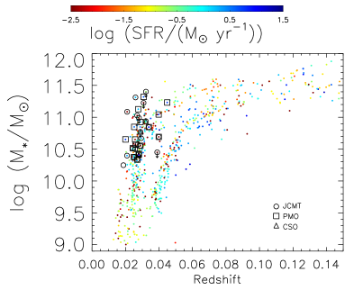
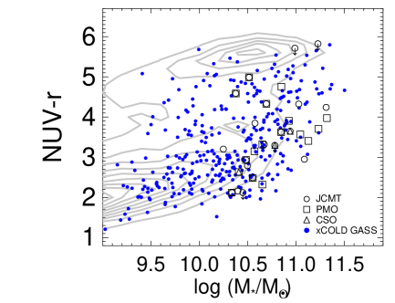
Figure 1: Distribution of our target galaxies on the plane of stellar mass versus redshift (left panel) and the plane of NUV$-r$ color versus stellar mass (right panel). In both panels, the open circles, squares and triangles represent our targets that are observed with the JCMT, PMO and CSO respectively. Symbols with a downward arrow represent CO upper limits from our JCMT observations. Small filled circles in the left panel show the MaNGA MPL-3 sample for comparison, color-coded by star formation rate taken from Salim et al. (2016). Blue dots in the right panel show CO detections from the xCOLD GASS survey, while the grey contours show the distribution of a volume-limited galaxy sample selected from the SDSS/DR7 main galaxy sample.

2 Sample and Observations

2.1 Target selection

Our parent sample is selected from the MaNGA Product Launch 3 (MPL-3), the latest MaNGA sample available when this work was initiated. The MPL-3 included $720$ galaxies with redshifts $z<0.15$ and stellar masses above $\sim 10^{9}$ M_⊙. It is a random subset of the 10,000 galaxies planned for the full MaNGA survey (Bundy et al., 2015). The MaNGA survey sample was selected from the Sloan Digital Sky Survey (SDSS) spectroscopic sample, mainly to have a flat distribution of $i$-band absolute magnitudes and for the assigned integral-field unit bundles to reach 1.5 or 2.5 effective radii ($R_{\rm e}$). The MaNGA sample design and optimisation is described in detail in Wake et al. (2017). The left panel of Figure 1 shows all the galaxies from the MaNGA MPL-3 on the plane of $\log$($M_{\ast}$) versus redshift, color-coded by the star formation rate (SFR) taken from Salim et al. (2016). The galaxies are distributed on two separate loci, corresponding to the two radius limits adopted in the MaNGA sample selection, i.e. 1.5 and 2.5 $R_{\rm e}$. Considering both the limited capability of our telescopes and the limited observing time, we restrict ourselves to low-redshift massive galaxies with redshifts $z<0.05$ and stellar masses $M_{\ast}$ $>10^{10}$ M_⊙. This restriction gives rise to a parent sample of 281 galaxies.

We have utilized three telescopes, the PMO 13.7-m telescope, the JCMT and CSO in Hawaii to obtain CO spectra for our target galaxies. We select targets from the same parent sample as described above, but for the three telescopes independently considering the following aspects. Firstly, the three telescopes have quite different sensitivities. JCMT is the most sensitive for a given observing time, while PMO is much less sensitive and so can only observe the brightest targets. Secondly, the PMO telescope can observe only the CO(1-0) line, while JCMT and CSO observe the CO(2-1) line. It is hard to construct a homogeneous sample of galaxies by obtaining CO observations for different galaxies from different telescopes. Therefore, we decided to first select a parent sample from the MaNGA survey, and then perform CO observations for three sub-samples of galaxies, each using one of the three telescopes independently. In this way, we expect to have some targets that are observed by more than one telescope, and these observations will be helpful both to cross-check the flux calibration of the different telescopes and to probe the ratio between the CO(2-1) and CO(1-0) lines.

For the PMO 13.7-m telescope, we select 17 galaxies that are brightest in the 12 µm, with the WISE W3 flux $f_{\mbox{12\micron}}$> 28 mJy. We detected CO(1-0) emission in all the 17 galaxies with a signal to noise ratio $S/N\geq$ 3. For the JCMT, we randomly selected a subset of the parent sample, but requiring that the total observing time per target required to reach $S/N=5$ must not exceed 5 hours, assuming Band 4 weather conditions. For this purpose we have estimated the observing time for each galaxy in MaNGA MPL-3 using the $L_{\mathrm{CO}}$-$L_{\mbox{12\micron}}$ relation from Jiang et al. (2015), and randomly select 21 out of 49 galaxies that meet the requirements. We detected CO(2-1) emission with $S/N\geq$ 3 in 16 galaxies, of which 7 are also observed with the PMO 13.7-m telescope. Finally, the CSO was used to obtain additional CO(2-1) observations for a small number of galaxies that are randomly selected from the parent sample without considering the observations at the other two telescopes. Due to the limited allocated time, only three galaxies are observed with this telescope, of which one is also observed with PMO, and two with JCMT. These observations are described in more detail in Section 2.2.

In summary, we have observed a sample of 31 galaxies using the three telescopes, of which 27 yielded a reliable detection. These 31 galaxies are highlighted in Figure 1 as black symbols, and their general properties including redshift, stellar mass, UV-to-optical color and infrared luminosity are listed in Table 1. In the right panel of Figure 1, we show the 31 galaxies in our sample on the plane of NUV$-r$ versus stellar mass. For comparison, we also show the xCOLD GASS sample galaxies (Saintonge et al., 2017) as blue dots which include 532 galaxies with CO(1-0) measurements from the IRAM (Institut de Radioastronomie Millimétrique) 30-m telescope, as well as a volume-limited galaxy sample selected from the SDSS main galaxy sample as grey contours which consists of 33,208 galaxies with redshifts $0.01<z<0.03$ and stellar masses $M_{\ast}>10^{9}$ M_⊙. Stellar masses, NUV$-r$ colors and redshifts for all galaxies in Figure 1 are taken from the NASA Sloan Atlas (NSA), a catalogue of images and parameters of more than 640,000 galaxies with $z<0.15$ from SDSS, as described in detail in Blanton et al. (2011).

As can be seen from Figure 1, our sample is limited to relatively massive galaxies with $M_{\ast}\gtrsim 2\times 10^{10}$ M_⊙. Our sample is also biased to blue colors when compared to the general population of galaxies from SDSS, but it appears to cover the NUV$-r$ space in a similar way to the galaxies detected in the xCOLD GASS survey.

Table 1: List of targets and their general properties.

Target No.	SDSS ID	$z$	$\log({\rm M}_{\ast}/{\rm M}_{\odot})$	NUV$-r$	$\log({\rm L}_{12\micron}/{\rm L}_{\odot})$	$\log({\rm L}_{22\micron}/{\rm L}_{\odot})$
				(mag)
1	J093637.19+482827.9	0.026	10.57	3.15 $\pm$ 0.06	9.80 $\pm$ 0.02	10.74 $\pm$ 0.03
2	J093106.75+490447.1	0.034	10.85	3.62 $\pm$ 0.07	9.82 $\pm$ 0.02	10.77 $\pm$ 0.03
3	J091554.70+441951.0	0.040	11.04	3.57 $\pm$ 0.05	10.11 $\pm$ 0.02	11.00 $\pm$ 0.03
4	J032057.90-002155.9	0.021	11.09	2.95 $\pm$ 0.06	9.40 $\pm$ 0.02	9.88 $\pm$ 0.03
5	J110158.99+451340.9	0.020	10.65	2.32 $\pm$ 0.05	9.46 $\pm$ 0.02	10.22 $\pm$ 0.03
6	J091500.75+420127.8	0.028	10.41	2.63 $\pm$ 0.05	9.59 $\pm$ 0.02	10.41 $\pm$ 0.03
7	J032043.20-010633.0	0.021	10.40	2.16 $\pm$ 0.05	9.10 $\pm$ 0.03	9.67 $\pm$ 0.03
8	J110637.35+460219.6	0.025	10.38	4.59 $\pm$ 0.06	9.37 $\pm$ 0.03	10.33 $\pm$ 0.03
9	J141225.99+454129.9	0.027	10.34	2.12 $\pm$ 0.06	9.34 $\pm$ 0.03	10.15 $\pm$ 0.03
10	J152950.65+423744.1	0.019	10.25	3.20 $\pm$ 0.05	8.64 $\pm$ 0.03	9.24 $\pm$ 0.03
11	J073749.42+462351.5	0.032	10.94	3.65 $\pm$ 0.05	9.39 $\pm$ 0.03	9.86 $\pm$ 0.03
12	J074442.28+422129.3	0.039	10.45	2.12 $\pm$ 0.05	9.45 $\pm$ 0.03	10.09 $\pm$ 0.03
13	J211557.49+093237.9	0.029	10.67	3.32 $\pm$ 0.08	9.44 $\pm$ 0.02	9.99 $\pm$ 0.03
14	J090015.61+401748.3	0.029	10.93	3.91 $\pm$ 0.07	9.34 $\pm$ 0.03	10.01 $\pm$ 0.03
15	J152625.50+422114.0	0.028	10.48	2.93 $\pm$ 0.05	9.38 $\pm$ 0.03	9.89 $\pm$ 0.03
16	J031345.21-001429.2	0.026	11.31	4.24 $\pm$ 0.05	9.22 $\pm$ 0.03	9.64 $\pm$ 0.03
17	J221134.29+114744.9	0.027	11.03	4.32 $\pm$ 0.05	9.17 $\pm$ 0.03	9.71 $\pm$ 0.03
18	J220943.19+133802.9	0.027	10.58	3.85	9.46 $\pm$ 0.02	10.01 $\pm$ 0.03
19	J171100.29+565600.9	0.029	10.55	2.49 $\pm$ 0.05	9.38 $\pm$ 0.03	10.01 $\pm$ 0.03
20	J093813.89+482317.9	0.026	10.50	2.79 $\pm$ 0.06	9.09 $\pm$ 0.03	9.58 $\pm$ 0.03
21	J072333.23+412605.6	0.028	11.13	3.41 $\pm$ 0.06	9.32 $\pm$ 0.03	9.80 $\pm$ 0.03
22	J110704.16+454919.6	0.025	10.85	4.75 $\pm$ 0.06	9.12 $\pm$ 0.03	9.73 $\pm$ 0.03
23	J092138.71+434334.2	0.040	10.69	4.33 $\pm$ 0.06	9.74 $\pm$ 0.03	10.33 $\pm$ 0.03
24	J121336.85+462938.2	0.026	10.65	3.32 $\pm$ 0.05	9.36 $\pm$ 0.03	9.81 $\pm$ 0.03
25	J074637.70+444725.8	0.031	11.32	3.97 $\pm$ 0.05	9.51 $\pm$ 0.02	9.94 $\pm$ 0.05
26	J134145.21+270016.9	0.029	10.78	3.29 $\pm$ 0.07	9.05 $\pm$ 0.03	9.40 $\pm$ 0.04
27	J103731.86+433913.7	0.024	10.51	4.99 $\pm$ 0.06	9.12 $\pm$ 0.03	9.54 $\pm$ 0.04
28	J083445.04+524256.4	0.045	11.23	3.71 $\pm$ 0.05	9.69 $\pm$ 0.03	10.04 $\pm$ 0.04
29	J103038.52+440045.7	0.028	10.99	5.71 $\pm$ 0.15	8.36 $\pm$ 0.05	8.40 $\pm$ 0.11
30	J171523.26+572558.3	0.032	11.40	12.62	8.13 $\pm$ 0.06	$\dots$
31	J110310.99+414219.0	0.031	11.23	5.82 $\pm$ 0.13	8.85 $\pm$ 0.06	$\dots$

Note. — From left to right, the columns are: (1) serial number unique to each target and kept the same in Table 2; (2) SDSS name formed by the R.A. and Dec. of the target; (3) optical redshift from SDSS; (4) & (5) stellar mass (a detailed discussion in Section 3.4) and NUV$-r$ color (and its uncertainty) from NSA; (6) & (7) mid-infrared luminosities at 12 and 22 µm (and their uncertainties) as measured by ourselves from the WISE images. There are two non-detections at 22µm.

2.2 CO Observations

Our observations of the CO(1-0) emission line at the PMO 13.7-m telescope were carried out over two periods in 2015, one from May 5th to June 1st, the other from November 6th to December 25th. These observations were taken with a nine-beam superconducting spectroscopic array receiver (Shan et al., 2012) with a main beam efficiency $\eta_{\rm mb}=0.513$ and a half–power beam width (HPBW) $\theta_{\rm HPBW}\sim 52^{\prime\prime}$. We have examined the optical size of our galaxies, as quantified by R₉₀ from the NSA (Blanton et al., 2011), the radius enclosing 90% of the total light in r-band, and we found more than 75% of our galaxies have a R₉₀ that is smaller than half of the HPBM of the PMO 13.7m telescope. In practice, the observations were made in ON-and-OFF mode. For each target galaxy, two of the nine beams were used, one covering the target and one pointing to an off-target area, thus simultaneously obtaining two short scans (each of 1 minute) of both the target and the background, that are then switched between the two beams. For each galaxy, we then combined a selected set of reliable scans to obtain the final integrated spectrum. For this, we visually examined all the scans, and discarded the spectra of scans with strongly distorted baselines, extremely large noise and/or any anomalous feature (mainly due to bad weather or high system temperature). We find the fraction of usable scans is $\sim$60% when the system temperature $T_{\rm sys}\lesssim 200$K, and decreases sharply at higher temperatures. The effective on-source time is $\sim$ 75 hours for the observations in the winter period, but only 95 minutes for those in May, although the actual allocated time was much longer in the latter period.

The observations of CO(2-1) at JCMT were taken from March to November in 2015 (project codes: M15AI28 and M15BI060; PI: Ting Xiao) with the RxA receiver in weather band 4 and 5. In total 16 hours of on-source time were allocated to the 21 target galaxies. RxA is a single receiver dual sideband (DSB) system, covering the frequency range 212 to 274 GHz, with $\eta_{\rm mb}=0.65$ and $\theta_{\rm HPBW}\sim 20^{\prime\prime}$ at 230 GHz. During these observations, the opacity $\tau$ at 225 GHz was less than 0.5. Once fully reduced, the observations yielded 16 detections and 5 non-detections for the 21 targeted galaxies.

At CSO, the CO(2-1) observations were obtained for the three target galaxies on 2015 February 19 and 20, using the heterodyne receiver with a full–width at half–maximum beam size of $30.\!{{}^{\prime\prime}}3\times 30.\!{{}^{\prime\prime}}7$ and a main beam efficiency of 76$\%$ at 230 GHz. For our observations, the typical system temperature ranged from 250 to 340 K, and the opacity $\tau$ was less than 0.2.

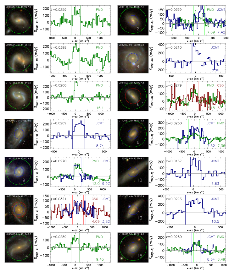
Figure 2: SDSS color images and CO spectra of our target galaxies. Each galaxy’s SDSS name and target number are overlaid on each image, while the telescope used and the $S/N$ are noted in the top-right and bottom-right corner of each spectrum. The green, blue and red circles overlaid on the images show the beam size of respectively PMO, JCMT and CSO as relevant. We used PMO to observe CO(1-0) and JCMT and CSO to observe CO(2-1). To directly compare the intensities from different telescopes, all spectra are in $S_{\rm CO(1-0)}$ units (assuming $R21$ = 0.7) and binned into channels $\sim$ 30 km s^-1 wide. The velocity scale displayed was obtained by subtracting the systemic velocity (redshift) from NSA catalogue. The vertical lines overplotted on the spectra indicate the velocity ranges (FWZI) of the CO emissions.

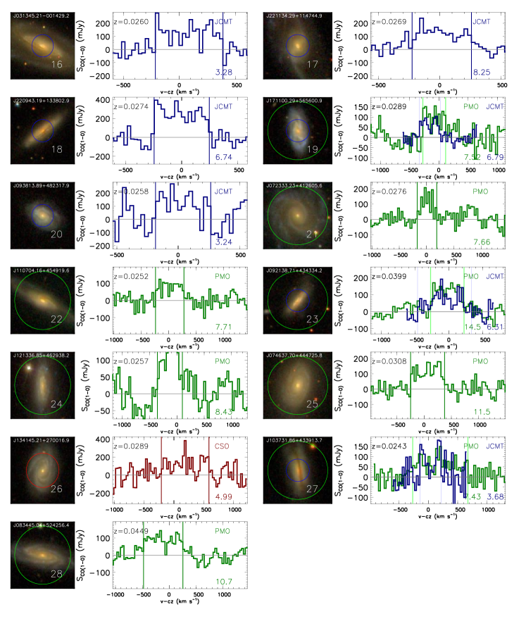
Figure 2: (Continued)

2.3 Data Reduction

We use the CLASS package to reduce the data obtained at PMO and CSO, part of the GILDAS software package (Pety, 2005). As described above, we visually examined all the scans and discarded unusable scans. In some of the selected scans, there are abnormally strong "line-like" features (stronger than 5 $\sigma$), where $\sigma$ is the root mean square (rms) noise. These spikes appear in individual original scans with channel width of $\delta v\sim$ 0.16 km s^-1; they contribute very little to the CO emission line measurement, but may affect the determination of the baseline. We replace the fluxes of the channels with spike features by the average flux of the neighbouring channels, following Tan et al. (2011). For a given galaxy, we then first obtain a linear baseline for each scan by fitting the spectrum over the full frequency range (except the expected range of the CO emission line), and subtract the fit from the spectrum. All the baseline-subtracted scans are then stacked to obtain an average spectrum of the galaxy. During the stacking, the different scans are weighted by the inverse of their rms noise. The STARLINK package (Currie et al., 2014) is used to reduce the JCMT data, with the default pipeline. We subtract the baselines to obtain the final spectra, that are then binned to a channel width of $\delta v\sim$ 30 km s^-1. The intensities are converted to main beam temperature $T_{\rm mb}$ from antenna temperature $T^{*}_{\rm A}$ using $T_{\rm mb}=T^{*}_{\rm A}/\eta_{\rm mb}$.

If a CO emission feature in the average spectrum appears significant, we select its velocity range manually as the full–width at zero–intensity (FWZI). We then measure the velocity-integrated CO line intensity, $I_{\rm CO}\equiv\int{T_{\rm mb}}\;dv$, by integrating the spectrum over this velocity range that reasonably covers the line feature. The uncertainty of the integrated intensity is estimated using the standard error formula in Gao (1996):

$$\Delta I_{\rm CO}\equiv T_{\rm rms}\Delta v_{\rm FWZI}\;/\;[f(1-\Delta v_{\rm FWZI}/W)]^{1/2},$$ (1)

where $T_{\rm rms}$ is the rms noise computed over the full spectrum (excluding the emission line), $f\equiv\Delta v_{\rm FWZI}/\delta v$ where $\Delta v_{\rm FWZI}$ is the FWZI of the emission feature and $\delta v$ the velocity channel width, and $W$ is the entire velocity coverage of the spectrum.

In cases where the CO line is undetected ($S/N<$3) or very weak, few of the targets have an Hi line width, so we compute a value of ${\Delta}I_{\rm CO}$ in the same way as above, but adopting a fixed FWZI of 300 km $\textrm{s}^{-1}$ following Saintonge et al. (2011). For these non-detections, an upper limit to the velocity-integrated intensity is then given as $3{\Delta}I_{\rm CO}$.

Assuming these galaxies are point-like sources, we convert the velocity-integrated line intensities in main beam brightness temperature ($T_{\rm mb}$) scale, i.e. $I_{\rm CO}$ as obtained above, to $S_{\rm CO}$, the CO line flux density in units of Jy km s^-1 using a conversion factor of 24.9, 18.4 and 40.2 Jy K^-1 for PMO, JCMT and CSO, respectively. Figure 2 displays the SDSS image (with the relevant telescope primary beam overlaid) and the final CO spectrum for the 27 detected galaxies in our sample. The spectra are plotted in terms of $S_{\rm CO(1-0)}$, that is the flux density of the CO (J=1-0) line. For the galaxies observed with JCMT or CSO, we have converted the CO (2-1) flux density to the CO (1-0) flux density assuming a CO(2-1)/CO(1-0) line ratio $R21$ = 0.7 (Leroy et al., 2013). In fact, the median $R21$ of the galaxies in our sample that have both CO(1-0) and CO(2-1) detections is also $\sim$0.7. For the galaxies observed by more than one telescope, we plot the spectra from the different telescopes with different colors. The repeated observations are generally in good agreement, in terms of both the intensity and width of the CO line.

Finally, we calculate the CO line luminosity following Bolatto et al. (2013):

$$\Big{(}\frac{L_{\rm CO}}{{\rm K\;km\;s}^{-1}\;{\rm pc^{2}}}\Big{)}=2453~{}\Big{(}\frac{S_{\rm CO}\Delta v}{{\rm Jy\;km\;s}^{-1}}\Big{)}\Big{(}\frac{D_{\rm L}}{\rm Mpc}\Big{)}^{2}(1+z)^{-1},$$ (2)

where $S_{\rm CO}\Delta v$ is the velocity integrated CO line flux density, $D_{\rm L}$ is the luminosity distance to the source, and $z$ is the source redshift from SDSS. The CO luminosity and corresponding uncertainty for each galaxy in our sample are listed in Table 2. For the galaxies observed by more than one telescope, we list the results from all the telescopes. In total, there are 41 observations including 36 detections for 27 galaxies, and 5 non-detections for 5 galaxies (1 galaxy has both a detection and a non-detection). Of the 31 galaxies, 10 were repeatedly observed: 7 with both PMO and JCMT, 2 with both JCMT and CSO, and 1 with both PMO and CSO. One galaxy with non-detection has a very blue color (NUV$-r$ $=2.12$) and a stellar mass of $M_{\ast}=10^{10.45}$ M_⊙ (target No. 11). This non-detection should be attributed to the relatively short integration of the observation due to our limited observing time.

We have attempted to correct the CO luminosities for the effect of the limited apertures of the telescopes. This aperture effect is negligible for the CO(1-0) observations obtained with the PMO 13.7-m telescope, that has a rather large beam size, larger than the optical diameter of our galaxies. In fact, following Saintonge et al. (2012), we estimated the ratio between the predicted total CO(1-0) flux and the flux observed within the beam, finding a median difference of less than 5% for PMO galaxies. Therefore, their CO flux can be nearly perfectly recovered with a single pointing, and we choose to not make a correction for these observations. For the CO(2-1) observations obtained with JCMT and/or CSO, the aperture effect cannot be ignored. We have thus performed an aperture correction for these observations adopting the method of Saintonge et al. (2012), based on the assumption that molecular gas within galaxies follows the same exponential profile as their stellar light. The correcting factors range from 1.05 to 1.96 (as shown in Table 2), and are included in all figures.

Table 2: Observed and derived properties of molecular gas for the target galaxies.

Target No.	Obs. No.	Telescope	Useful Exp.	$I_{\rm CO(1-0)}$	$I_{\rm CO(2-1)}$	$\log(L{{}^{\prime}}_{\rm CO(1-0)})$	$S_{\rm CO,tot}/S_{\rm CO,obs}$	log($M_{\rm mol}$)
			(min)	(K km s-1)	(K km s-1)	(${\rm K\;km\;s}^{-1}\;{\rm pc^{2}}$)		(M⊙)
1	1	PMO	55	1.75 $\pm$ 0.23	$\dots$	9.11 $\pm$ 0.06	$\dots$	9.74
2	2	PMO	358	1.21 $\pm$ 0.15	$\dots$	9.19 $\pm$ 0.06	$\dots$	9.82
	3	JCMT	48	$\dots$	5.36 $\pm$ 0.72	9.27 $\pm$ 0.06	1.15	9.96
3	4	PMO	54	2.07 $\pm$ 0.24	$\dots$	9.56 $\pm$ 0.05	$\dots$	10.19
4	5	JCMT	53.3	$\dots$	2.24 $\pm$ 0.58	8.47 $\pm$ 0.11	1.11	9.15
5	6	PMO	167	1.64 $\pm$ 0.11	$\dots$	8.86 $\pm$ 0.03	$\dots$	9.49
6	7	PMO	135	1.44 $\pm$ 0.18	$\dots$	9.09 $\pm$ 0.05	$\dots$	9.72
	8	CSO	6.7	$\dots$	2.28 $\pm$ 0.73	9.03 $\pm$ 0.14	1.05	9.68
7	9	JCMT	66.2	$\dots$	2.17 $\pm$ 0.25	8.45 $\pm$ 0.05	1.63	9.30
8	10	PMO	341	1.19 $\pm$ 0.16	$\dots$	8.91 $\pm$ 0.06	$\dots$	9.54
	11	JCMT	16	$\dots$	8.18 $\pm$ 1.09	9.19 $\pm$ 0.06	1.1	9.86
9	12	PMO	328	1.62 $\pm$ 0.14	$\dots$	9.11 $\pm$ 0.04	$\dots$	9.74
	13	JCMT	57.1	$\dots$	4.1 $\pm$ 0.41	8.95 $\pm$ 0.04	1.29	9.69
10	14	JCMT	80	$\dots$	1.6 $\pm$ 0.24	8.22 $\pm$ 0.07	1.65	9.07
11	15	JCMT	36.3	$\dots$	2.61 $\pm$ 0.68	8.91 $\pm$ 0.11	1.96	9.84
	16	CSO	30	$\dots$	1.21 $\pm$ 0.30	8.87 $\pm$ 0.11	1.39	9.65
12	17	JCMT	16.4	$\dots$	<3.58	<9.14	1.14	<9.83
13	18	JCMT	60.5	$\dots$	4.42 $\pm$ 0.42	9.06 $\pm$ 0.04	1.23	9.78
14	19	PMO	249	1.33 $\pm$ 0.14	$\dots$	9.09 $\pm$ 0.05	$\dots$	9.72
15	20	PMO	133	1.21 $\pm$ 0.14	$\dots$	9.02 $\pm$ 0.05	$\dots$	9.65
	21	JCMT	40	$\dots$	4.04 $\pm$ 0.47	8.98 $\pm$ 0.05	1.17	9.68
16	22	JCMT	60.5	$\dots$	2.82 $\pm$ 0.86	8.76 $\pm$ 0.13	1.7	9.62
17	23	JCMT	110.6	$\dots$	3.2 $\pm$ 0.39	8.84 $\pm$ 0.05	1.39	9.62
18	24	JCMT	40	$\dots$	6.3 $\pm$ 0.94	9.15 $\pm$ 0.06	1.28	9.89
19	25	PMO	51	1.68 $\pm$ 0.22	$\dots$	9.19 $\pm$ 0.06	$\dots$	9.82
	26	JCMT	68	$\dots$	3.01 $\pm$ 0.44	8.88 $\pm$ 0.06	1.27	9.62
20	27	JCMT	32	$\dots$	2.95 $\pm$ 0.91	8.77 $\pm$ 0.13	1.22	9.49
21	28	PMO	204	1.58 $\pm$ 0.21	$\dots$	9.12 $\pm$ 0.06	$\dots$	9.75
22	29	PMO	207	1.66 $\pm$ 0.21	$\dots$	9.06 $\pm$ 0.06	$\dots$	9.69
23	30	PMO	141	2.61 $\pm$ 0.18	$\dots$	9.66 $\pm$ 0.03	$\dots$	10.29
	31	JCMT	26.3	$\dots$	8.33 $\pm$ 1.32	9.60 $\pm$ 0.07	1.14	10.29
24	32	PMO	130	1.93 $\pm$ 0.23	$\dots$	9.15 $\pm$ 0.05	$\dots$	9.78
25	33	PMO	89	2.96 $\pm$ 0.26	$\dots$	9.49 $\pm$ 0.04	$\dots$	10.12
26	34	JCMT	52.6	$\dots$	<1.29	<8.51	1.49	<9.32
	35	CSO	23	$\dots$	2.11 $\pm$ 0.42	9.02 $\pm$ 0.09	1.26	9.75
27	36	PMO	137	2.55 $\pm$ 0.34	$\dots$	9.22 $\pm$ 0.06	$\dots$	9.85
	37	JCMT	16	$\dots$	4.32 $\pm$ 1.18	8.89 $\pm$ 0.12	1.4	9.67
28	38	PMO	132	2.67 $\pm$ 0.25	$\dots$	9.78 $\pm$ 0.04	$\dots$	10.41
29	39	JCMT	26.3	$\dots$	<1.69	<8.60	1.27	<9.34
30	40	JCMT	49.4	$\dots$	<1.68	<8.72	3.27	<9.35
31	41	JCMT	16	$\dots$	<2.5	<8.85	1.82	<9.74

Note. — From left to right, the columns are: (1) serial number unique to the target; (2) serial number of the observation; (3) telescope used for the observation; (4) on-source observing time; (5)&(6) CO(1-0) or CO(2-1) integrated intensity (and its uncertainty) of the CO emission line; (7) derived CO(1-0) luminosity (and its uncertainty) without aperture correction; (8) aperture corrections for the CO(2-1) observations; (9)molecular gas mass (and its uncertainty) after aperture correction, which is computed as introduced in Section 4.1.

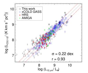
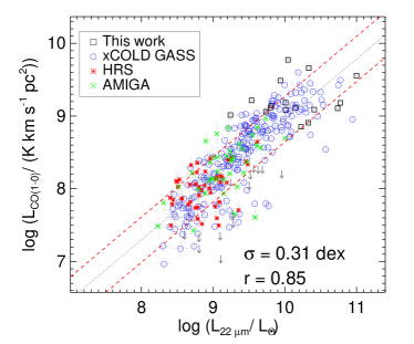
Figure 3: Correlation of the CO(1-0) luminosities with the mid-infrared luminosities from WISE measured in the 12 (left panel) and 22 µm (right panel) band . Different colors/symbols indicate detections in different CO samples, as indicated in the top-left corner of each panel, and the grey error bars to show their measurement uncertainties, while the dark grey downward-pointing arrows mean upper limits from xCOLD GASS. In each panel, the dotted black line and two dashed red lines show respectively the best-fitting linear relation (with parameters listed in Table 3) and the $1\sigma$ total/observed scatter for detections only obtained from all the samples together. The total/observed scatter ($\sigma$) and the Spearman’s correlation coefficient ($r$) for all the detections are listed in the bottom-right corner of each panel.

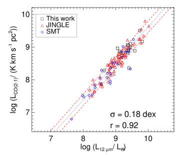
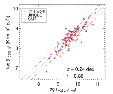
Figure 4: As Figure 3, but for the CO(2-1) luminosities.

3 Correlations between the CO and MIR luminosities

In this section we first examine the correlations of the CO (1-0) and CO (2-1) luminosities with the mid-infrared luminosities from the WISE 12µm and 22µm bands. We then extend the correlation of the CO(1-0) luminosity with the 12 µm luminosity to derive an estimator of the CO(1-0) luminosity, by considering other galaxy properties as additional parameters to the 12 µm luminosity. Finally we apply this estimator to our galaxies with only CO(2-1) observations, as well as those from the JINGLE and SMT surveys, examining the dependence of the CO(2-1)-to-(1-0) line ratio on a variety of galaxy properties.

We have measured the 12 and 22 µm luminosities of all the galaxies to be included in the following analyses. For each galaxy we reprocessed the W3 (12 µm) and W4 (22 µm) images from WISE using the SEXTRACTOR package (Bertin & Arnouts, 1996). We manually adjusted the shape and size of the ellipse to properly cover the MIR emission of each galaxy. Before estimating the fluxes and luminosities, we carefully masked out by hand foreground and background sources as well as neighboring galaxies identified in the corresponding SDSS image. We used redshift from SDSS when computing the distance. The 12 and 22 µm luminosities (and their respective uncertainties) thus estimated for our galaxies are listed in Table 1, with median uncertainties of 0.021 and 0.026 dex, respectively. The uncertainty includes both the photometric uncertainty (is consistent with flux uncertainty in WISE catalog) and the uncertainty of the magnitude zero-point (Jarrett et al., 2011).

3.1 Correlations between CO and mid-infrared luminosities

Figure 3 shows the correlation of the CO(1-0) luminosities, $L_{\rm CO(1-0)}$, with the mid-infrared luminosities measured from WISE in the 12 (left panel) and 22 µm  (right panel) band. Our galaxies observed with the PMO 13.7-m telescope are plotted as black squares. For comparison, we show the detected galaxies from xCOLD GASS (Saintonge et al., 2017), HRS (Boselli et al., 2014) and AMIGA (Lisenfeld et al., 2011), that have significant detections in both CO(1-0) and WISE ($S/N$ > 3), as blue circles, red stars and green crosses, respectively. The figure thus includes all types of galaxies, early- and late-type galaxies as well as active galactic nucleus (AGN) hosts, interacting/paired galaxies and luminous infrared galaxies (LIRGs). Analogously, Figure 4 shows the correlation of the CO(2-1) luminosities, $L_{\rm CO(2-1)}$, with the WISE 12 and 22 µm  luminosities. Our galaxies detected with JCMT and/or CSO are plotted as black squares, while those detections from JINGLE (Saintonge et al., 2018) and the SMT observations of Jiang et al. (2015) are plotted as red triangles and blue diamonds, respectively.

Table 3: Best-fit relations between CO and MIR luminosities.

${\rm log}(L_{\mbox{12\micron}}{\rm L_{\odot}})$	${\rm log}(L_{\rm CO}/[{\rm K\;km\;s}^{-1}\;{\rm pc^{2}}])$	Sample	k	b	$\sigma_{\rm int}$	corresponding panel
12 µm	CO(1-0)	CO detections (412)	0.98 $\pm$ 0.02	-0.14 $\pm$ 0.18	0.20	the left panel of Figure 3
12 µm	CO(1-0)	CO detections and upper limits (565)	1.03 $\pm$ 0.02	-0.64 $\pm$ 0.18	0.21
12 µm	CO(2-1)	CO detections (118)	1.11 $\pm$ 0.04	-1.52 $\pm$ 0.33	0.15	the left panel of Figure 4
22 µm	CO(1-0)	CO detections (318)	0.83 $\pm$ 0.03	0.63 $\pm$ 0.30	0.30	the right panel of Figure 3
22 µm	CO(1-0)	CO detections and upper limits (332)	0.84 $\pm$ 0.03	0.50 $\pm$ 0.32	0.33
22 µm	CO(2-1)	CO detections (114)	0.94 $\pm$ 0.04	-0.47 $\pm$ 0.44	0.21	the right panel of Figure 4

Notes. The relations are parametrized as $y=kx+b$, with all the quantities given in this table. The number of galaxies included in the fitting is indicated in parenthesis in the sample column. The derived intrinsic scatter of each relation is listed as $\sigma_{\rm int}$.

As one can see from Figure 3, our galaxies are located in the upper-right corner of both panels, with the highest CO(1-0) and MIR luminosities, slightly extending the trend defined by existing observations towards high luminosities. This is expected as our PMO sample was selected to be brightest in the 12 µm band. In Figure 4, our galaxies appear to span a similar range of CO(2-1) luminosities as the JINGLE sample galaxies at mid-to-high end, although with less coverage at both the high- and low-luminosity ends due to the much smaller sample size. This is again understandable, as we selected our JCMT targets randomly from the parent sample.

From Figures 3 and 4, we see that the CO and MIR luminosities are well-correlated in all cases, but the correlations are tighter and more linear when the MIR luminosity is measured in the 12 µm band rather than the 22 µm band. This is true for both the CO(1-0) and CO(2-1) lines. To quantify this effect, we performed a Bayesian linear regression of $L_{\rm CO}$ as a function of MIR luminosity at both 12µm and 22µm, taking into account uncertainties in both the x and y axes using LinMix (Kelly, 2007), implemented in the IDL script linmix_err.pro. In each panel of Figures 3 and 4, we plot the best-fit line to detections only and the $1\sigma$ scatter (i.e. the standard deviation of the data points around the fit) about each line. The scatters are $\sigma=$ 0.22, 0.31, 0.18 and 0.24 dex, and the Spearman’s correlation coefficients are 0.93, 0.85, 0.92 and 0.86, respectively, for the correlation of $L_{\rm CO(1-0)}$ vs. $L_{\mbox{12\micron}}$, $L_{\rm CO(1-0)}$ vs. $L_{\mbox{22\micron}}$, $L_{\rm CO(2-1)}$ vs. $L_{\mbox{12\micron}}$ and $L_{\rm CO(2-1)}$ vs. $L_{\mbox{22\micron}}$, as indicated in each panel. The parameters of the best-fitting relations are listed in Table 3 including the derived intrinsic scatters. For the relations with $L_{\rm CO(1-0)}$, we also carried out fits taking into account non-detections in xCOLD GASS (as "censored" data), and the fitting results do not change significantly.

The fits suggest that the MIR luminosities are slightly more tightly correlated with the CO(2-1) luminosities than with the CO(1-0) luminosities. This can be easily understood, as CO(2-1) is associated with denser and/or warmer gas than CO(1-0), and is thus more likely to be associated with the star-formation traced by the MIR luminosities. As the CO(1-0) observations come from several different telescopes/surveys, the slightly larger scatters in the correlations of the CO(1-0) observations could also be partly (if not fully) attributed to the systematic differences between the different samples. In particular, the CO(2-1) observations in Figure 4 are dominated by the JINGLE sample. For the CO(1-0) observations, the total/observed (intrinsic) scatter is reduced to 0.20 (0.18) dex if we consider only the xCOLD GASS sample. The K-correction of the MIR luminosities probably also partly contributes to the scatter in these relations (see Lee et al., 2013).

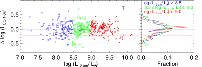
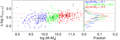
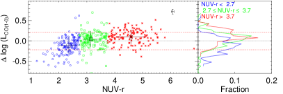
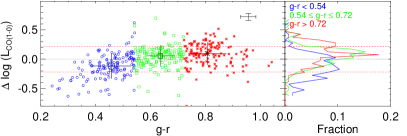
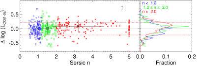
Figure 5: In the left-hand panels, for CO(1-0) detections, we plot the residuals (${\Delta}$ log($L_{\rm CO(1-0)})\equiv$ log($L_{\rm CO(1-0),obs}$)- log($L_{\rm CO(1-0),est}$)) of CO(1-0) luminosity predicted from the best-fitting relation (Eq. 3) between $L_{\rm CO(1-0)}$ and $L_{12\micron}$ and the observed $L_{\rm CO(1-0)}$ as a function of 12 µm luminosity $L_{12\micron}$, stellar mass $M_{\ast}$  NUV$-r$ color, $g-r$ color and Sersic index $n$ (from top to bottom). The dashed red horizontal lines show the $1\sigma$ total/observed scatter of all galaxies, and the characteristic error bars illustrate the median value of available measurement uncertainties. In each panel, we divide the galaxies into 3 sub-samples (with the same number of galaxies in each) according to the parameter considered. Blue circles, green squares and red stars correspond to respectively the smallest, intermediate and largest parameter values, and the large symbols show the median and scatter in each bin. In the right-hand panels, the different colors show the distribution of the residuals in each sub-sample.

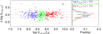
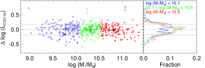
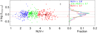
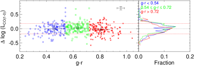
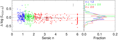
Figure 6: As Figure 5 but for the residuals of the predicted value of $L_{\rm CO(1-0)}$ using the three-parameter estimator (Eq. 4).

On the other hand, we notice that another more important reason for the larger total/observed and intrinsic scatters in the $L_{\rm CO(1-0)}$ correlations is the systematic deviation of some of the low-luminosity galaxies, many being well below the linear relation of the whole sample. As can be clearly seen in Figure 3, this effect occurs mainly at $L_{\mbox{12\micron}}\lesssim 10^{8}$ L_⊙and $L_{\mbox{22\micron}}\lesssim 10^{9}$ L_⊙. The CO(2-1) samples contain very few galaxies at these luminosities. When data become available in the future, it would thus be interesting to see whether the $L_{\rm CO(2-1)}$ versus MIR luminosity correlations also show similar downturns at the low-luminosity end.

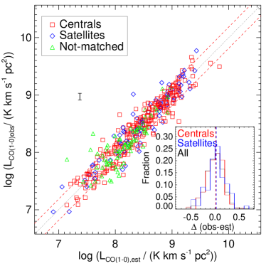
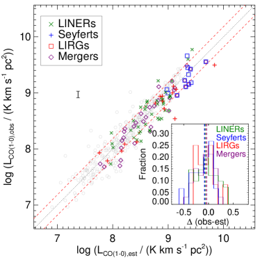
Figure 7: New estimator of the CO(1-0) luminosity ($L_{\rm CO(1-0)}$) based on $L_{12\micron}$, $M_{\ast}$ and $g-r$, as well as the distribution of the residuals of some sub-samples. In each panel, the dotted black line and two dashed red lines show respectively the best-fitting relation (with parameters listed in Table 4) and the $1\sigma$ total/observed scatter (0.18 dex) of all galaxies. In the left panel, different symbols/colors are used to highlight any difference between central and satellite galaxies. In the right panel, we highlight particular galaxy populations including BPT-selected AGN hosts (LINERs as dark green crosses and Seyferts as blue plus signs), LIRGs (red squares) and interacting galaxies or mergers (purple diamonds). In insets, the histograms and vertical dashed lines show respectively the distributions and median values of the residuals for different sub-samples.

3.2 Residuals in the CO vs. MIR luminosity relation

To better understand the scatters and the systematic deviations discussed above (Section 3.1) in relation to the CO versus 12 µm luminosity relations, we hereby examine the residuals about the best-fitting relations as a function of a variety of galaxy parameters. As a byproduct, this analysis is expected to produce a new estimator of CO(1-0) luminosity, that is a linear combination of multiple parameters, thus providing estimated CO(1-0) luminosities with smaller uncertainties and biases than those estimated from the 12 µm luminosity alone.

We primarily consider the linear fit between $L_{\rm CO(1-0)}$ and $L_{\mbox{12\micron}}$, that is

$$\textrm{log}\Big{(}\frac{L_{\rm CO(1-0)}}{{\rm K\;km\;s}^{-1}\;{\rm pc^{2}}}\Big{)}=(0.98\pm 0.02)\textrm{log}\Big{(}\frac{L_{12\micron}}{\rm L_{\odot}}\Big{)}-(0.14\pm 0.18),$$ (3)

as indicated in the left panel of Figure 3. In Figure 5 we plot the residual of the CO(1-0) luminosity as a function of five different galaxy parameters (from top to bottom) for all available galaxies: 12 µm-band luminosity ($L_{\mbox{12\micron}}$), stellar mass ($M_{\ast}$), $NUV-r$ color, $g-r$ color and Sersic index ($n$). The residual is defined as the logarithm of the ratio of the observed CO(1-0) luminosity to the estimated one. In this case, a positive (negative) residual indicates a higher (lower) molecular gas mass than that predicted by $L_{\mbox{12\micron}}$. Optical colors and the $NUV-r$ color are known to be sensitive to the cold gas fraction of galaxies (Saintonge et al., 2011), while the Sersic index is a structural parameter whereby larger $n$ indicate earlier-type morphologies (and a prominent bulge for late-type galaxies). In each panel, galaxies in different bins of the parameter considered are plotted with different symbols/colors. The two red dotted horizontal lines in each panel indicate the $1\sigma$ scatter of all the sample galaxies about the best-fitting relation, $0.22$ dex in this case. To the right of each panel we add a smaller panel showing the histogram of the $L_{\rm CO(1-0)}$ residuals for the three sub-samples including the same number of objects defined by the parameter considered.

Overall, the residuals are constant about zero with no/weak dependence for $L_{\mbox{12\micron}}$ (as expected) and the Sersic index $n$, but are significantly negative for galaxies with the lowest masses (${M_{\ast}}\lesssim 10^{10}$ M_⊙) and bluest colors (NUV$-r$ $\lesssim 3$ and/or $g-r\lesssim 0.5$). This echoes the downturn at the low-luminosity end seen above in the $L_{\rm CO(1-0)}-L_{\mbox{12\micron}}$ relation (Figure 3).

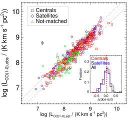
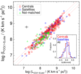
Figure 8: As Figure 7 but for alternative estimators of the CO(1-0) luminosity ($L_{\rm CO(1-0)}$) based on $L_{12\micron}$, $g-r$ color and $r$–band luminosity (left); $L_{12\micron}$, $g-r$ color and $z$– band luminosity (center); $L_{12\micron}$ , $r$–and $z$–band luminosities (right). The characteristic error bars shown illustrate the median (direct or derived) measurement uncertainties.

3.3 A three-parameter estimator of CO(1-0) luminosity

We therefore include the stellar mass and $g-r$ color as additional parameters, and estimate $L_{\rm CO(1-0)}$ using LinMix (see above) over multiple parameters ($L_{\rm 12\micron}$, $M_{\ast}$ and $g-r$) as provided in Table 4:

$$\begin{split}\textrm{log}\Big{(}\frac{L_{\rm CO(1-0)}}{{\rm K\;km\;s}^{-1}\;{\rm pc^{2}}}\Big{)}=(0.76\pm 0.03)\textrm{log}\Big{(}\frac{L_{12\micron}}{\rm L_{\odot}}\Big{)}+(0.29\pm 0.04)(g-r)\\ +(0.29\pm 0.08)\textrm{log}\Big{(}\frac{M_{\ast}}{\rm M_{\odot}}\Big{)}-(1.41\pm 0.25).\end{split}$$ (4)

Figure 6 shows the residuals of the CO(1-0) luminosities predicted by this 3-parameter estimator as a function of $L_{\mbox{12\micron}}$, $M_{\ast}$, NUV$-r$, $g-r$ and Sersic index $n$, in the same manner as Figure 5. The residuals show no dependence on any parameter. The additional two parameters also improve a bit the estimate for the high-mass or red galaxies, though which are used to mainly remove the residuals in low mass and blue galaxies. The total/observed scatter of all the galaxies about the best-fitting relation is 0.18 dex, considerably smaller than the scatter of 0.22 dex when estimating $L_{\rm CO(1-0)}$ from the 12µm luminosity alone.

One might wonder whether it is necessary to include both $M_{\ast}$ and $g-r$ as additional parameters. In fact, we have attempted to add only one parameter, either $M_{\ast}$ or NUV$-r$ or $g-r$, in addition to the 12µm luminosity, and we find none of them taken alone can provide unbiased estimates. A third parameter is always necessary to remove systematic biases, although it does not help to significantly reduce the scatter. We have also examined a 3-parameter estimator combining $L_{\mbox{12\micron}}$, $M_{\ast}$ and NUV$-r$, i.e. replacing $g-r$ by NUV$-r$ in Eq. 4. We find the estimator using $g-r$ works better, yielding smaller biases and slightly smaller scatter.

One may also worry about possible biases in the CO(1-0) luminosities of galaxies located in different environments, that were previously shown to influence the cold gas content of galaxies (e.g. Li et al., 2012; Zhang et al., 2013). In the left panel of Figure 7, we compare the observed CO luminosities of the galaxies in this work with those predicted by our estimator, showing the results for central galaxies (red squares) and satellite galaxies (blue diamonds) differently (unmatched galaxies are shown as green triangles). The central/satellite classification is taken from the SDSS galaxy group catalog constructed by Yang et al. (2007) in which the central galaxy of a given group of galaxies is defined to be the most massive galaxy in the group. The inset shows the histograms of the residuals for both central and satellite galaxy subsets; there is no obvious bias. We also carry out a Kolmogorov-Smirnov (K$-$S) test between the residuals of the centrals/satellites and those of the total sample. The K$-$S probability (p-value) is 0.98 and 0.41, respectively, suggesting the two samples to be drawn from the same parent sample randomly.

In the right-hand panel of Figure 7, we show the same relation again, but using different symbols/colors to differentiate the subsets of Seyfert galaxies, LINERs (low ionization nuclear emission regions), LIRGs and merging galaxies. The identification of Seyferts and LINERs is done using the Baldwin, Phillips & Terlevich (BPT) diagram (Baldwin et al., 1981), adopting the AGN classification curve of Kauffmann et al. (2003) and the Seyfert-LINER dividing line of Cid Fernandes et al. (2010). The relevant emission-line ratios are taken from the Max-Planck-Institute for Astrophysics-John Hopkins University (MPA-JHU) SDSS database (Brinchmann et al., 2004). The LIRGs in our sample are identified according to their infrared luminosity over 8–1000 µm, $L_{8-1000\mbox{\micron}}$. To this end, we first estimate the infrared luminosity over 40–500 µm, $L_{40-500\mbox{\micron}}$, based on the luminosities at 60 and 100 µm from the Infrared Astronomical Satellite (IRAS) database (Moshir et al., 1992) according to Sanders & Mirabel (1996, see their Table 1), and then convert $L_{40-500\mbox{\micron}}$ to $L_{8-1000\mbox{\micron}}$ adopting a conversion factor of 1.75 following Hopkins et al. (2003). The identification of interacting galaxy systems is similar to Lin et al. (2004). In short, two close galaxies are classified as a pair and included in the subset of interacting systems if their projected separation is < 50 $h^{-1}$ kpc and their line-of-sight velocity difference is < 500 km s^-1. Additional interacting systems are identified by visually inspecting the SDSS images. We again compare their distributions of residuals with that of the total sample, and K$-$S test returns a p-value = 0.23, 0.21, 0.66 and 0.24 for LINERs, Seyfert, LIRGs and mergers, respectively. Again, there is no/weak differences between different types of galaxies in the right panel of Figure 7.

These results demonstrate that Eq. 4 provide unbiased estimator of the CO luminosity of a galaxy, and can thus be applied to large samples of galaxies for which CO observations are not available.

Table 4: Best-fit relations for three-parameter molecular gas mass estimators.

$x_{2}$ parameter	$x_{3}$ parameter	$k_{1}$	$k_{2}$	$k_{3}$	b	$\sigma_{\rm int}$	corresponding panel
$g-r$	log $({M_{\ast}}/{\rm M_{\odot}})$	0.77 $\pm$ 0.03	0.29 $\pm$ 0.08	0.28 $\pm$ 0.04	-1.40 $\pm$ 0.24	$\dots$	Figure 7
$g-r$	log $({L_{r}}/{\rm L_{\odot}})$	0.82 $\pm$ 0.03	0.55 $\pm$ 0.06	0.18 $\pm$ 0.03	-0.94 $\pm$ 0.21	0.16	the left panel of Figure 8
$g-r$	log $({L_{z}}/{\rm L_{\odot}})$	0.81 $\pm$ 0.03	0.47 $\pm$ 0.06	0.20 $\pm$ 0.03	-0.99 $\pm$ 0.20	0.16	the middle panel of Figure 8
log $({L_{r}}/{\rm L_{\odot}})$	log $({L_{z}}/{\rm L_{\odot}})$	0.79 $\pm$ 0.03	-1.89 $\pm$ 0.22	2.07 $\pm$ 0.21	-0.72 $\pm$ 0.21	0.15	the right panel of Figure 8

Notes. The relations are parametrized as log $(L_{\rm CO(1-0)}/({\rm K\;km\;s}^{-1}\;{\rm pc^{2}}))=k_{1}log~{}(L_{\mbox{12\micron}}/{\rm L_{\odot}})+k_{2}x_{2}+k_{3}x_{3}+b$, with all the quantities given in this table. The derived intrinsic scatter of each relation is listed as $\sigma_{\rm int}$.

3.4 Alternative estimators

It should be noted that the estimators mentioned in Section 3.3 can only be used with $M_{\ast}$ measured in the same manner as that used here, i.e. NSA $M_{\ast}$, as there are significant systematic uncertainties/biases on $M_{\ast}$ associated with the different methods and assumptions used to infer it (e.g. stellar initial mass function IMF and population models; e.g. Bell et al., 2003; Li & White, 2009). In addition, for these estimators, we can not separate the intrinsic scatter from the total/observed scatter (as shown in Table 4), as the NSA catalogue does not include a random/measurement uncertainty on $M_{\ast}$ for each galaxy. According to the analysis of different stellar masses estimated in different manner based on similar IMF, the typical uncertainty is about 0.15 - 0.2 dex, but it increases substantially at lower masses, reaching 0.3 dex at $10^{8}$ $h^{-2}$ M_⊙. We therefore provide other estimators using instead the $r$– and/or $z$– band stellar luminosities in Table 4, that are not subject to these large systematic effects and are less dependent on stellar population models.

These relations, shown in Figure 8, arise naturally from the data through multiple-parameter linear regression fitting, without any assumption. All of these estimators appear to be similarly good, with small total/observed scatters of $\sim$ 0.18 dex (intrinsic scatters of $\sim$ 0.16 dex) and no obvious difference between central and satellite galaxies.

3.5 The CO(2-1)-to-CO(1-0) line ratio $R21$

Here we present an immediate application of the $L_{\rm CO(1-0)}$ estimator (Eq. 4), whereby we estimate the CO(1-0) luminosity of galaxies that have only CO(2-1) observations and then investigate the inferred CO(2-1)-to-CO(1-0) line ratios ($R21$). For this purpose we have compiled a sample of galaxies with CO(2-1) but no CO(1-0) observations, including 72 galaxies from JINGLE (Saintonge et al., 2018), 27 from the SMT sample of Jiang et al. (2015), and 10 from our own sample (see Table 2). We first estimate the CO(1-0) luminosity of each galaxy from its 12µm luminosity, stellar mass and $g-r$ color according to Eq. 4, and then infer $R21$ from the ratio of the observed CO(2-1) luminosity to the estimated CO(1-0) luminosity. For comparison, we also consider two samples of galaxies from previous studies where both CO(1-0) and CO(2-1) integrated fluxes are available:18 galaxies from the HERA CO-Line Extragalactic Survey (HERACLES; Leroy et al., 2009), and 27 xCOLD GASS galaxies with detections in both IRAM CO(1-0) and APEX CO(2-1) measurements (Saintonge et al., 2017).

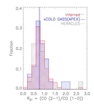
Figure 9: Distribution of CO(2-1)-to-CO(1-0) line ratios for the inferred (based on observed $L_{\rm CO(2-1)}$ and predicted $L_{\rm CO(1-0)}$) and observed (literature) samples. The red histogram shows the inferred $R21$, while the blue and gray histograms show the observed xCOLD GASS (with APEX) and HERACLES survey, respectively. The colored vertical lines indicate the median $R21$ of each sample.

Figure 9 shows the histogram of the inferred $R21$ (red), compared to those of the observed $R21$ from the two previous studies considered (blue and gray). It is encouraging to see that the $R21$ distribution based on our estimates agrees very well with the real observations, that are also in good agreement with each other. This is true in terms of both the median $R21$ of the samples and the overall shape of the distributions. The median $R21$ is 0.78 for the inferred sample, very close to the median value of 0.75 and 0.77 for xCOLD GASS and HERACLES. The $1\sigma$ widths of the distributions are also very similar, 0.17, 0.18 and 0.18 dex, respectively. The K$-$S test yields p-value of 0.96 and 0.76 for xCOLD GASS and HERACLES, respectively, suggesting the probabilities are larger than 75% that they are drawn from the same sample. Finally, we nevertheless notice a tail of galaxies with higher-than-average $R21$ in both xCOLD GASS and HERACLES, dominated by merging systems. The only such galaxy in our inferred sample is also a merging galaxy. Given the relatively small sample sizes, however, this different fraction of higher-than-average $R21$ should not be overemphasized.

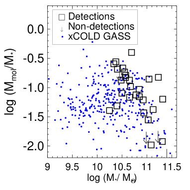
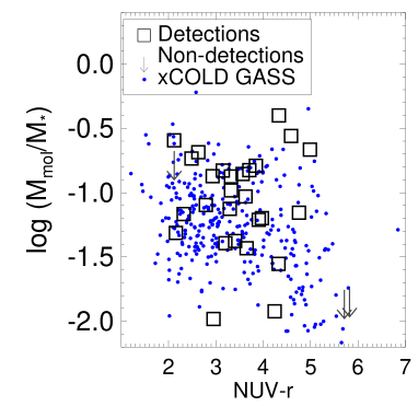
Figure 10: Distribution of our sample galaxies on the planes of molecular-to-stellar mass ratio log $(M_{\rm mol}/M_{\ast})$ versus log $(M_{\ast})$ (middle) and log $(M_{\rm mol}/M_{\ast})$ versus NUV$-r$ (right). In each panel, our galaxies are plotted as large symbols (black squares for CO detections and downward-pointing arrows for upper limits), while the detections from the xCOLD GASS survey are plotted as blue dots.

4 Total molecular gas content $M_{\rm mol}$

In this section we examine the correlation of molecular gas mass fraction with star formation rate, using both real gas masses from our sample and the xCOLD GASS and estimated gas masses for the current MaNGA sample obtained from the three-parameter CO (1-0) luminosity estimator as presented in Section 3.3.

4.1 $M_{\rm mol}$ of our sample

For the galaxies observed with the PMO 13.7-m telescope, we estimate the total molecular gas mass by multiplying the CO (1-0) luminosity (corrected for aperture effect) by a CO-to-H₂ conversion factor: $M_{\rm mol}=\alpha_{\rm CO}L_{\rm CO(1-0)}$. A Galactic conversion factor $\alpha_{\rm CO}=4.3$ M_⊙(K km s${}^{-1}{\rm pc^{2}})^{-1}$ corresponding to $X_{\rm CO}=2\times 10^{20}$ cm^-2 (K km s${}^{-1})^{-1}$ is adopted, so the resulting molecular gas mass includes a factor of 1.36 for the presence of heavy elements (mainly helium). For the galaxies observed with JCMT or CSO, we convert their CO (2-1) luminosities to CO (1-0) luminosities assuming a CO (2-1)/CO (1-0) line ratio of $R21=0.7$ following Leroy et al. (2013), and we caculate the total molecular gas mass in the same manner as above. Although slightly smaller than the median values of the samples studied in the previous section (Section 3.5), the line ratio of $R21=0.7$ is adopted for the convenience of potential comparisons of our results with the literature. The H₂ masses are listed in the last column of Table 2.

Figure 10 shows the molecular-to-stellar mass ratio $M_{\rm mol}$/$M_{\ast}$ as a function of respectively stellar mass $M_{\ast}$ and NUV$-r$ color, this for both our galaxies and the xCOLD GASS detections. Although biased to massive gas-rich galaxies, our sample spans wide ranges in both NUV$-r$ and $M_{\rm mol}$/$M_{\ast}$, similarly to the xCOLD GASS sample galaxies, which allows the statistical analyses presented below.

4.2 Correlation of $M_{mol}$ with star formation rate

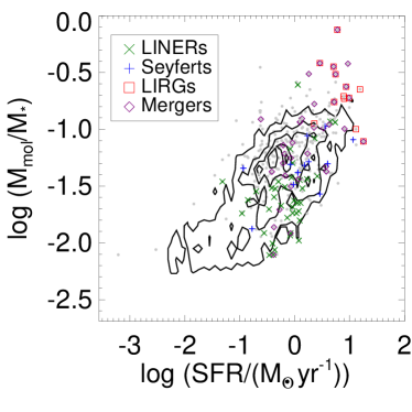
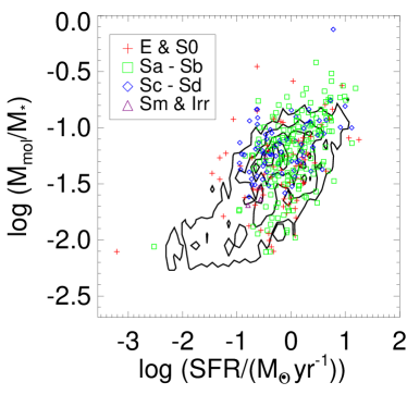
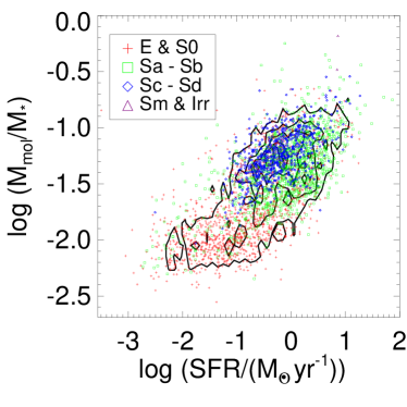
Figure 11: Distribution of galaxies on the plane of molecular gas-to-stellar mass ratio versus star formation rate. The upper panels show the distribution of our sample and xCOLD GASS with observed gas masses, and the lower panels show the distribution of the MaNGA/MPL-8 sample for which the gas masses are estimated using our three-parameter $L_{\mbox{CO(1-0)}}$ estimator (Eq. 4). Different colors/symbols represent different types of galaxies (left) or different morphologies (right), as indicated. Black contours show the distribution of the whole MaNGA/MPL-8 sample, repeated in every panel for comparison.

Hereby we persent an application of our CO estimator to the current sample of the MaNGA survey, the MaNGA/MPL-8 sample which consists of 6,487 galaxies. In most cases CO observation is not available. In particular, we focus on the correlation of molecular gas-to-stellar mass ratio, $M_{\rm mol}$/$M_{\ast}$ with the star formation rate (SFR). We estimate an H₂ mass for each galaxy in MaNGA/MPL-8 using our three-parameter $L_{\mbox{CO(1-0)}}$ estimator (see Eq. 4), and we make use of the $M_{\ast}$ and SFR estimates from the GALEX-SDSS-WISE Legacy Catalog (GSWLC; Salim et al., 2016, 2018) for this analysis. As in Section 3.3, the galaxies are divided into subsets of LINERs, Seyfert galaxies, LIRGs and merging galaxies, as well as subsets of different morphological types according to Hubble type from the HyperLeda database (Makarov et al., 2014). For comparison we also include in the analysis the xCOLD GASS and our sample which have observed molecular gas masses.

In Figure 11 we show the distributions of different types of galaxies in the $M_{\rm mol}$/$M_{\ast}$—SFR plane. The top panels display the galaxies from the xCOLD GASS and our sample, but highlighting subsets of LINERs/Syeferts/LIRGs/Mergers with different symbols/colors in the left panel and subsets of different morphologies in the right panel. The lower panels display the MaNGA/MPL-8 sample, highlighting the different subsets in the same manner as the upper panels. The black contours present the distribution of all MPL-8 galaxies, and are repeated in every panel for comparison.

We see that, overall, $M_{\rm mol}$/$M_{\ast}$ is positively correlated with SFR in all panels, as expected. When comparing the samples with real gas mass fractions with the MaNGA/MPL-8 sample with estimated gas mass fractions, we find similar correlations and scatters in the upper-right part of the diagram ($\log(M_{\mbox{mol}}/M_{\ast})\gtrsim-2$ and $\log SFR\gtrsim-1$) where data is available for both samples. This is true not only for the whole samples, but also for subsamples of different types. LIRGs are expectably located in the upper-right corner with highest SFRs and molecular gas fractions. Other types of galaxies span a wide range in both SFR and $M_{\mbox{mol}}/M_{\ast}$, but present systematic differences. For instance, at given SFR, merging galaxies appear to be more gas-rich than LINERs, while Seyfert galaxies are found in between; on average Sc and Sd-type spirals are more gas-rich than earlier morphological types which are distributed more broadly and scatteringly. These trends are more clearly seen in the lower panels thanks to the much larger sample sizes.

A remarkable difference between the real gas samples and the estimated gas samples occurs in the lower-left part of the panels where the MaNGA sample extends well below the detection limit of the xCOLD GASS, thus adding a significant population of gas-poor galaxies to this diagram which are predominantly early-type (E or S0). In contrast to the gas-rich galaxies from xCOLD GASS, the gas-poor population presents almost no correlation between the molecular gas mass fraction and the SFR, although their SFR spands a wide range from $\log(SFR/M_{\odot}{\mbox{yr}}^{-1})\sim-1$ to $\sim-3$. The lower-left panel shows that the majority of these galaxies are LINERs, while many mergers and some Seyferts also fall in this regime. The mergers should be dry mergers given their relatively low gas fractions. All these trends are interesting, and deserve more detailed analyses. In the next work we will come back to the MaNGA sample, and we will combine the estimated global molecular gas mass with integral field spectroscopy to better understand the role of cold gas in driving the star formation and nuclear activity of galaxies.

5 Summary and Discussion

We have obtained CO(1-0) and/or CO(2-1) spectra for a sample of 31 galaxies selected from the ongoing MaNGA survey. We utilized three different telescopes: PMO 13.7-m millimeter telescope located in Delingha, China, CSO and JCMT located in Hawaii. We measured the total CO flux/luminosities and molecular gas masses of our galaxies. Combining our sample with other samples of CO observations from the literature, we examined the correlations of the CO luminosities with the infrared luminosities at 12 ($L_{\mbox{12\micron}}$) and 22 µm ($L_{\mbox{22\micron}}$). We then examined the residuals of the $L_{\rm CO(1-0)}$-$L_{\mbox{12\micron}}$ relation as a function of a variety of galaxy properties including stellar mass ($M_{\ast}$), color (NUV$-r$ and $g-r$) and Sersic index ($n$), to find a linear combination of multiple parameters that may be used to estimate molecular gas masses for large samples of galaxies.We applied the resulting best-fitting estimator to a sample of galaxies with only CO (2-1) observations and investigated the resulting CO(2-1)-to-CO(1-0) ratios, as well as the current sample of MaNGA to study the correlation of molecular gas-to-stellar mass ratio as a function of SFR, galaxy type and morphology.

Our main conclusions can be summarized as follows:

1. Our sample consists of 31 relatively massive galaxies with stellar masses $\gtrsim 2\times 10^{10}$ M_⊙, spanning all morphological types and covering wide ranges of colors and molecular gas-to-stellar mass ratios, that are similar to those of the xCOLD GASS sample.

2. The CO luminosities are tightly correlated with the MIR luminosities, and the correlation with the 12 µm band has a smaller scatter and is more linear than the one with the 22 µm band. The $L_{\rm CO(1-0)}$–$L_{\mbox{12\micron}}$ relation shows no/weak dependence on the MIR luminosities and Sersic indices, while galaxies with the lowest masses and/or bluest colors are below the mean relation.

3. A linear combination of the 12 µm-band luminosity $L_{\mbox{12\micron}}$, stellar mass ($M_{\ast}$) and optical color $g-r$ provides unbiased estimates of the CO(1-0) luminosities (and thus molecular gas masses). This estimator works well for both central and satellite galaxies, and for different types of galaxies such as LIRGs, Seyferts, LINERs and mergers. Replacing $M_{\ast}$ by the luminosity in the $r$ or $z$ band yields similarly good estimators.

4. The distribution of $R21$ obtained from estimated CO(1-0) luminosities agrees well with real measurements from previous studies. The median $R21$ of this inferred sample is $R21=0.78$, with a scatter of 0.17 dex, consistent with the typical value of 0.7 that is commonly-adopted in previous studies.

5. Applying our $L_{\mbox{CO(1-0)}}$ estimator to $\sim 6,400$ galaxies in the current sample of MaNGA, we find a significant population of gas-poor galaxies which are predominantly early-type. The molecular gas-to-stellar mass ratio of these galaxies shows no correlation with star formation rate, in contrast to gas-rich galaxies that have been previously studied in depth.

The tight correlation between CO luminosity and 12 µm luminosity was already reported and studied in some detail by Jiang et al. (2015). This correlation is not unexpected, given both the tight relation between the surface densities of star formation rate and cold gas mass, known as the Kennicutt-Schmidt law (Schmidt, 1959; Kennicutt, 1998), and the correlations of SFR with infrared luminosities. For the latter, in particular, Donoso et al. (2012) found that $\sim$ 80% of the 12 µm emission from star-forming galaxies in the WISE survey is produced by stellar populations younger than $\sim$ 0.6 Gyr, implying a strong correlation of SFR with the 12 µm luminosity.

When compared to $L_{\mbox{12\micron}}$, the luminosities at 22µm show larger scatter and a more non-linear correlation with the CO luminosities. This is true for both CO(1-0) and CO(2-1) (see Figures 3 and 4). Assuming the SFR is the driving factor for the correlations of $L_{\rm CO}$ with MIR luminosities, this result implies that the 12 µm luminosity is a better indicator of star formation than the 22 µm luminosity. This may be understood from the fact that the W3 band of WISE, which spans a wavelength range from 7.5 to 16.5 µm, includes and is almost centered on the prominent polycyclic aromatic hydrocarbon (PAH) emission at 11.3 µm (Wright et al., 2010), and that our sample does not include any strong AGN (e.g. quasar). The mid-infrared spectra from the Spitzer Infrared Nearby Galaxies Survey (SINGS; Kennicutt et al., 2003), as obtained by the Spitzer Infrared Spectrograph (Houck et al., 2004), revealed that the PAH emission can contribute up to $\sim 20\%$ of the total infrared emission. In addition, both the dust continuum emission and the PAH emission are well correlated with CO emission (Wilson et al., 2000; Cortzen et al., 2019), while the W4 band of WISE may detect stochastic emission from heated small grains with temperatures of $\sim\ 100-150$ K (in addition to the Wien tail of thermal emission from large grains; Wright et al., 2010).

The $L_{\rm CO(1-0)}$–$L_{\mbox{12\micron}}$ relation should in principle provide a very useful estimator, that can be easily applied to estimate the molecular gas masses of large samples of galaxies, particularly considering the all-sky survey data from WISE and the small scatter ($\sim$ 0.2 dex) of the relation. In fact, this simple estimator has been successfully applied by the JINGLE team to estimate observing times for the purpose of target selection (Saintonge et al., 2018). In this work, we have further improved the estimator by including two more parameters, $M_{\ast}$ and $g-r$, that are also available for large samples of galaxies thanks to the imaging data from SDSS and other large optical surveys. We have shown that such estimators provide unbiased CO luminosity estimates for different types of galaxies. Our new three-parameter estimator will be helpful to provide more accurate estimates of molecular gas masses and thus to study gas-related processes in a wider range of galaxies than currently possible (e.g. gas-poor galaxies and gas-related quenching processes; e.g. Li et al., 2012; Zhang et al., 2013). As an example, in this paper we have performed a quick application of our estimator to the current MaNGA sample (MPL-8), and found a significant population of gas-poor galaxies that fall below the detection limit of existing CO surveys (e.g. xCOLD GASS). This population is dominated by early-type galaxies and shows no correlation between $M_{\mbox{mol}}/M_{\ast}$ and SFR, differently from gas-rich galaxies which show a strong correlation. We will come back to the MaNGA sample in future works and combine our estimated gas masses with the MaNGA integral field spectroscopy to better understand this gas-poor population.

Appendix A The capability of PMO to detect external galaxies

Figure 12: Fraction of usable scans taken with the PMO telescope as a function of the system temperature. The diamonds and error bars are the mean and $1\sigma$ scatter of the fraction within each $T_{\rm sys}$ bin.

The PMO 13.7-m telescope has traditionally been mostly used to observe Galactic sources (e.g. Ma et al., 2019) or extra-galactic sources in the very nearby Universe ($z<0.01$; e.g. Li et al., 2015). All our targets are beyond $z=0.01$. Our work is thus the first attempt to observe a sample of non-local galaxies with this telescope. Therefore, this is a good opportunity to test the capability of PMO to detect external galaxies. We find the fraction of usable scans to strongly depend on the system temperature, $T_{\rm sys}$. This is clearly shown in Figure 12, where we plot the fraction of selected scans as a function of $T_{\rm sys}$. The fraction is roughly constant at 60% when $T_{\rm sys}\lesssim 200$ K, but it decreases dramatically at higher temperatures. At $T_{\rm sys}>220$ K, the observation efficiency is very low, with only $20-30\%$ of usable scans. Figure 12 shows that the PMO telescope can be effectively used to observe external galaxies, as long as the system temperature is lower than $\sim 200$ K. Our observations were carried out in two period, one in May and one in winter. Typically, the system temperature in the winter period of our observations ranges from 150 to 220 K. In May, however, the situation is already much worse, with a mean of $T_{\rm sys}\sim 200$ K. Therefore, most of the discarded scans were taken in May (after around mid-May). In total, the effective on-source time is $\sim$ 75 hours for the observations in the winter period, but only 95 minutes for those in May, although the actual allocated time was much longer in the latter period.

References

- Baldwin et al. (1981) Baldwin, J. A., Phillips, M. M., & Terlevich, R. 1981, PASP, 93, 5
- Bell et al. (2003) Bell, E. F., McIntosh, D. H., Katz, N., & Weinberg, M. D. 2003, ApJS, 149, 289
- Bertin & Arnouts (1996) Bertin, E., & Arnouts, S. 1996, A&AS, 117, 393
- Bigiel et al. (2008) Bigiel, F., Leroy, A., Walter, F., et al. 2008, AJ, 136, 2846
- Blanton et al. (2011) Blanton, M. R., Kazin, E., Muna, D., Weaver, B. A., & Price-Whelan, A. 2011, AJ, 142, 31
- Bolatto et al. (2008) Bolatto, A. D., Leroy, A. K., Rosolowsky, E., Walter, F., & Blitz, L. 2008, ApJ, 686, 948
- Bolatto et al. (2013) Bolatto, A. D., Wolfire, M., & Leroy, A. K. 2013, ARA&A, 51, 207
- Boselli et al. (2014) Boselli, A., Cortese, L., & Boquien, M. 2014, A&A, 564, A65
- Brinchmann et al. (2013) Brinchmann, J., Charlot, S., Kauffmann, G., et al. 2013, MNRAS, 432, 2112
- Brinchmann et al. (2004) Brinchmann, J., Charlot, S., White, S. D. M., et al. 2004, MNRAS, 351, 1151
- Bundy et al. (2015) Bundy, K., Bershady, M. A., Law, D. R., et al. 2015, ApJ, 798, 7
- Carilli & Walter (2013) Carilli, C. L., & Walter, F. 2013, ARA&A, 51, 105
- Catinella et al. (2010) Catinella, B., Schiminovich, D., Kauffmann, G., et al. 2010, MNRAS, 403, 683
- Cid Fernandes et al. (2010) Cid Fernandes, R., Stasińska, G., Schlickmann, M. S., et al. 2010, MNRAS, 403, 1036
- Cortzen et al. (2019) Cortzen, I., Garrett, J., Magdis, G., et al. 2019, MNRAS, 482, 1618
- Currie et al. (2014) Currie, M. J., Berry, D. S., Jenness, T., et al. 2014, in Astronomical Society of the Pacific Conference Series, Vol. 485, Astronomical Data Analysis Software and Systems XXIII, ed. N. Manset & P. Forshay, 391
- Donoso et al. (2012) Donoso, E., Yan, L., Tsai, C., et al. 2012, ApJ, 748, 80
- Eales et al. (2012) Eales, S., Smith, M. W. L., Auld, R., et al. 2012, ApJ, 761, 168
- Eckert et al. (2015) Eckert, K. D., Kannappan, S. J., Stark, D. V., et al. 2015, ApJ, 810, 166
- Erb et al. (2006) Erb, D. K., Shapley, A. E., Pettini, M., et al. 2006, ApJ, 644, 813
- Gao (1996) Gao, Y. 1996, PhD thesis, STATE UNIVERSITY OF NEW YORK AT STONY BROOK
- Gao & Solomon (2004) Gao, Y., & Solomon, P. M. 2004, ApJ, 606, 271
- Giovanelli et al. (2005) Giovanelli, R., Haynes, M. P., Kent, B. R., et al. 2005, AJ, 130, 2598
- Groves et al. (2015) Groves, B. A., Schinnerer, E., Leroy, A., et al. 2015, ApJ, 799, 96
- Hopkins et al. (2003) Hopkins, A. M., Miller, C. J., Nichol, R. C., et al. 2003, ApJ, 599, 971
- Houck et al. (2004) Houck, J. R., Roellig, T. L., van Cleve, J., et al. 2004, ApJS, 154, 18
- Israel (1997) Israel, F. P. 1997, A&A, 328, 471
- Jarrett et al. (2011) Jarrett, T. H., Cohen, M., Masci, F., et al. 2011, The Astrophysical Journal, 735, 112
- Jiang et al. (2015) Jiang, X.-J., Wang, Z., Gu, Q., Wang, J., & Zhang, Z.-Y. 2015, ApJ, 799, 92
- Kannappan (2004) Kannappan, S. J. 2004, ApJ, 611, L89
- Kannappan et al. (2013) Kannappan, S. J., Stark, D. V., Eckert, K. D., et al. 2013, ApJ, 777, 42
- Kauffmann et al. (2003) Kauffmann, G., Heckman, T. M., Tremonti, C., et al. 2003, MNRAS, 346, 1055
- Kelly (2007) Kelly, B. C. 2007, ApJ, 665, 1489
- Kennicutt (1998) Kennicutt, Robert C., J. 1998, ApJ, 498, 541
- Kennicutt et al. (2003) Kennicutt, Robert C., J., Armus, L., Bendo, G., et al. 2003, PASP, 115, 928
- Kokusho et al. (2017) Kokusho, T., Kaneda, H., Bureau, M., et al. 2017, A&A, 605, A74
- Kokusho et al. (2019) —. 2019, A&A, 622, A87
- Komatsu et al. (2011) Komatsu, E., Smith, K. M., Dunkley, J., et al. 2011, ApJS, 192, 18
- Kruijssen (2014) Kruijssen, J. M. D. 2014, Classical and Quantum Gravity, 31, 244006
- Lee et al. (2013) Lee, J. C., Hwang, H. S., & Ko, J. 2013, ApJ, 774, 62
- Leroy et al. (2008) Leroy, A. K., Walter, F., Brinks, E., et al. 2008, AJ, 136, 2782
- Leroy et al. (2009) Leroy, A. K., Walter, F., Bigiel, F., et al. 2009, AJ, 137, 4670
- Leroy et al. (2011) Leroy, A. K., Bolatto, A., Gordon, K., et al. 2011, ApJ, 737, 12
- Leroy et al. (2013) Leroy, A. K., Walter, F., Sandstrom, K., et al. 2013, AJ, 146, 19
- Li et al. (2012) Li, C., Kauffmann, G., Fu, J., et al. 2012, MNRAS, 424, 1471
- Li & White (2009) Li, C., & White, S. D. M. 2009, MNRAS, 398, 2177
- Li et al. (2015) Li, F.-C., Wu, Y.-W., & Xu, Y. 2015, Research in Astronomy and Astrophysics, 15, 785
- Lin et al. (2004) Lin, L., Koo, D. C., Willmer, C. N. A., et al. 2004, ApJ, 617, L9
- Lisenfeld et al. (2011) Lisenfeld, U., Espada, D., Verdes-Montenegro, L., et al. 2011, A&A, 534, A102
- Ma et al. (2019) Ma, Y. J., Toth, G., Nagy, A. F., & Russell, C. T. 2019, in Lunar and Planetary Science Conference, Lunar and Planetary Science Conference, 2903
- Magdis et al. (2011) Magdis, G. E., Daddi, E., Elbaz, D., et al. 2011, ApJ, 740, L15
- Makarov et al. (2014) Makarov, D., Prugniel, P., Terekhova, N., Courtois, H., & Vauglin, I. 2014, A&A, 570, A13
- McKee & Ostriker (2007) McKee, C. F., & Ostriker, E. C. 2007, ARA&A, 45, 565
- Moshir et al. (1992) Moshir, M., Kopman, G., & Conrow, T. A. O. 1992, IRAS Faint Source Survey, Explanatory supplement version 2
- Paturel et al. (2003) Paturel, G., Theureau, G., Bottinelli, L., et al. 2003, A&A, 412, 57
- Pety (2005) Pety, J. 2005, in SF2A-2005: Semaine de l’Astrophysique Francaise, ed. F. Casoli, T. Contini, J. M. Hameury, & L. Pagani, 721
- Rafieferantsoa et al. (2018) Rafieferantsoa, M., Andrianomena, S., & Davé, R. 2018, MNRAS, 479, 4509
- Riechers et al. (2019) Riechers, D. A., Pavesi, R., Sharon, C. E., et al. 2019, ApJ, 872, 7
- Saintonge et al. (2011) Saintonge, A., Kauffmann, G., Kramer, C., et al. 2011, MNRAS, 415, 32
- Saintonge et al. (2012) Saintonge, A., Tacconi, L. J., Fabello, S., et al. 2012, ApJ, 758, 73
- Saintonge et al. (2017) Saintonge, A., Catinella, B., Tacconi, L. J., et al. 2017, ApJS, 233, 22
- Saintonge et al. (2018) Saintonge, A., Wilson, C. D., Xiao, T., et al. 2018, MNRAS, 481, 3497
- Salim et al. (2018) Salim, S., Boquien, M., & Lee, J. C. 2018, ApJ, 859, 11
- Salim et al. (2016) Salim, S., Lee, J. C., Janowiecki, S., et al. 2016, ApJS, 227, 2
- Sanders & Mirabel (1996) Sanders, D. B., & Mirabel, I. F. 1996, ARA&A, 34, 749
- Sandstrom et al. (2013) Sandstrom, K. M., Leroy, A. K., Walter, F., et al. 2013, ApJ, 777, 5
- Schmidt (1959) Schmidt, M. 1959, ApJ, 129, 243
- Scoville et al. (2014) Scoville, N., Aussel, H., Sheth, K., et al. 2014, ApJ, 783, 84
- Shan et al. (2012) Shan, W., Yang, J., Shi, S., et al. 2012, IEEE Transactions on Terahertz Science and Technology, 2, 593
- Shi et al. (2016) Shi, Y., Wang, J., Zhang, Z.-Y., et al. 2016, Nature Communications, 7, 13789
- Solomon et al. (1987) Solomon, P. M., Rivolo, A. R., Barrett, J., & Yahil, A. 1987, ApJ, 319, 730
- Tacconi et al. (2018) Tacconi, L. J., Genzel, R., Saintonge, A., et al. 2018, ApJ, 853, 179
- Tan et al. (2011) Tan, Q.-H., Gao, Y., Zhang, Z.-Y., & Xia, X.-Y. 2011, Research in Astronomy and Astrophysics, 11, 787
- Tremonti et al. (2004) Tremonti, C. A., Heckman, T. M., Kauffmann, G., et al. 2004, ApJ, 613, 898
- Wake et al. (2017) Wake, D. A., Bundy, K., Diamond-Stanic, A. M., et al. 2017, AJ, 154, 86
- White & Rees (1978) White, S. D. M., & Rees, M. J. 1978, MNRAS, 183, 341
- Wilson et al. (2000) Wilson, C. D., Scoville, N., Madden, S. C., & Charmandaris, V. 2000, ApJ, 542, 120
- Wright et al. (2010) Wright, E. L., Eisenhardt, P. R. M., Mainzer, A. K., et al. 2010, AJ, 140, 1868
- Yang et al. (2007) Yang, X., Mo, H. J., van den Bosch, F. C., et al. 2007, ApJ, 671, 153
- Yesuf et al. (2017) Yesuf, H. M., French, K. D., Faber, S. M., & Koo, D. C. 2017, MNRAS, 469, 3015
- Zhang et al. (2013) Zhang, W., Li, C., Kauffmann, G., & Xiao, T. 2013, MNRAS, 429, 2191
- Zhang et al. (2009) Zhang, W., Li, C., Kauffmann, G., et al. 2009, MNRAS, 397, 1243
- Zu (2018) Zu, Y. 2018, arXiv e-prints, arXiv:1808.10501
- Zwaan et al. (2005) Zwaan, M. A., Meyer, M. J., Staveley-Smith, L., & Webster, R. L. 2005, MNRAS, 359, L30