Charged dust close to outer mean-motion resonances in the heliosphere

Abstract

We investigate the dynamics of charged dust close to outer mean-motion resonances with planet Jupiter. The importance of the interplanetary magnetic field on the orbital evolution of dust is clearly demonstrated. New dynamical phenomena are found that do not exist in the classical problem of uncharged dust. We find changes in the orientation of the orbital planes of dust particles, an increased amount of chaotic orbital motions, sudden ’jumps’ in the resonant argument, and a decrease in time of temporary capture due to the Lorentz force. Variations in the orbital planes of dust grain orbits are found to be related to the angle between the orbital angular momentum and magnetic axes of the heliospheric field and the rotation rate of the Sun. These variations are bound using a simplified model derived from the full dynamical problem using first order averaging theory. It is found that the interplanetary magnetic field does not affect the capture process, that is still dominated by the other non-gravitational forces. Our study is based on a dynamical model in the framework of the inclined circular restricted three-body problem. Additional forces include solar radiation pressure, solar wind drag, the Poynting-Robertson effect, and the influence of a Parker spiral type interplanetary magnetic field model. The analytical estimates are derived on the basis of Gauss’ form of planetary equations of motion. Numerical results are obtained by simulations of dust grain orbits together with the system of variational equations. Chaotic regions in phase space are revealed by means of Fast Lyapunov Chaos Indicators.

Keywords Charged dust, mean-motion resonance, temporary capture, chaos

1 Introduction

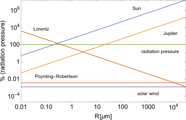
Figure 1: Magnitudes of forces (evaluated using (2), (3), (6) at $8[AU]$ with dust grain density $2.8[g/cm^{3}]$, and surface charge $5[V]$) in $\%$ of force due to solar radiation pressure versus dust grain diameter $R$ (in microns). We assume slow solar wind conditions with mean solar wind speed equal $400[km/s]$, and mean background magnetic field strength defined at $1[AU]$ to be equal $3[nT]$.

Dust in space is subject to various non-gravitational forces originating from stellar radiation, i.e. due to the interaction of dust with solar photons, the solar wind, as well as the heliospheric magnetic field. The magnitudes of these forces do not only depend on the position and velocity of these grains relative to the central star, but also on their physical and chemical composition (Kimura and Mann, 1998). The orbital motion of dust is clearly affected by the magnetic field in interplanetary space (Morfill and Gruen, 1979; Gruen et al., 1994). However, the role of it on motion close to mean motion-resonances is still unclear. Previous studies (Sicardy et al., 1993; Beauge and Ferraz-Mello, 1994; Beauge, 1994; Liou and Zook, 1997; Jancart et al., 2003; Klačka and Kocifaj, 2008; Pástor et al., 2009; Kocifaj and Kundracik, 2012; Pástor, 2014; Lhotka and Celletti, 2015; Pástor, 2016) investigated the dynamical problem under the assumption that dust is uncharged. This assumption is only valid in the case where the dust grain is heavy enough and where the magnitude of the Lorentz force is much smaller compared to the magnitudes of the other ones. However, for sub-micron and micron sized particles this assumption is clearly invalid as can already be seen in Fig. 1. The figure compares the magnitudes of different forces that act on the orbit of micron-sized dust grains in our solar system: gravitational attraction of the Sun and Jupiter, solar radiation, force due to the Poynting-Robertson effect and solar wind drag, as well as the Lorentz force. We clearly see that Lorentz force starts as the dominant force for submicron sized particles until radiation pressure, solar attraction, and the force related to charge become similar in magnitude around $R=0.2[\mu m]$. Electro-magnetic force decreases further for larger particles until it becomes of the same order as Jupiter’s gravity (around $3[\mu m]$). Interestingly enough, force related to charge is still larger in magnitude than the other non-gravitational effects, that are usually taken into account in these kinds of studies: solar wind drag and the force due to the Poynting-Robertson effect. For the choice of our parameters, Lorentz force becomes smaller in magnitude than these other non-gravitational forces around $1[cm]$. The figure clearly demonstrates the importance of the interplanetary magnetic field on charged-particle dynamics. In recent years, the effect of the interplanetary magnetic field on dust motion has already been included in Kocifaj et al. (2006), where the authors studied the role of temperature-dependent optical properties on the life-time of dust particles. In Lhotka et al. (2016), the authors investigated the role of the normal component of the heliospheric magnetic field on the stability of dust motion in interplanetary space. Both fore-mentioned studies excluded the phenomenon of resonant capture of dust. The charging history of dust grains is strongly influenced by the surrounding space plasma environment: currents due to the presence of free electrons and ions, secondary electron emission, and the photoelectric effect are known to be the dominant charging effects in interplanetary space (Popel et al., 2018; Mann et al., 2014; Popel et al., 2011; Popel and Gisko, 2006). In studies of dusty plasmas the current balance equation allows to model the charge history of dust grains on time-scales relevant for plasma physicists. Simulation studies show that charge of dust grains becomes constant if the sum over all currents (from and to the surrounding space plasma) vanishes. The existence of stationary solutions enables us to investigate long-term phenomena, i.e. the stability of dust grain orbits, in interplanetary space with the assumption of constant charge. However, it should be noted that all results based on this assumption are only valid as long as we assume consistency of the surrounding space plasma environment. This is the case in the current study. We assume a positive constant charge of dust grains solely due to the photoelectric effect. We thus neglect variations in time of the charging process. For additional information, also see Shukla and Mamun (2002).

The aim of the current study is to investigate the influence of the interplanetary magnetic field on charged dust grain orbits close to outer mean-motion resonances. Special focus is made to test the results in Beauge and Ferraz-Mello (1994) in presence of an additional Lorentz force term in the equations of motion of the dust particles. Our study is based on a simple dynamical formulation of the problem, i.e. the circular, inclined, restricted three-body problem. However, we also include various non-gravitational effects, which are all detailed in Sec. 2. For the interplanetary magnetic field we assume the validity of a Parker spiral model (Parker, 1958; Meyer-Vernet, 2012) throughout the solar system, i.e. we neglect the effect of solar cycle variations, solar flares, or coronal mass ejections. Already this very simple formulation of the magnetic field in the heliosphere allows us to demonstrate its effects on the orbits of charged dust grains: 1. A strong influence on the inclination and ascending node of the orbital planes of the dust grains with respect to the inertial plane, which is strongly related to the separation angle between the magnetic axis and the direction of the angular momentum. 2. A ’jumping’ effect of the resonant argument due to additional perturbations. 3. A decrease in capture time due to the increased level of chaotic regions in phase space close to resonance.

The model description can be found in Sec. 2, the isolated influence of the magnetic field on the orientation of the orbital plane is described in Sec. 3. The detailed numerical study of the unaveraged equations of motion is provided in Sec. 4. The main results are summarized and discussed in Sec. 5.

2 Model and Methodology

We consider a micrometer-sized dust particle orbiting in our solar system. We study its orbital evolution by taking into account the gravity and the forces due to the interaction of the dust grain with the solar radiation and the interplanetary medium. We refer to the motion of the particle in a heliocentric, ecliptic reference frame, $\mathcal{G}_{Sun}=\{\vec{g}_{x},\vec{g}_{y},\vec{g}_{z}\}$, were $\vec{g}_{z}$ is directed to the ecliptic pole, $\vec{g}_{x}$ is aligned with the direction to the vernal equinox, and $\vec{g}_{y}$ completes the right handed set. The equation of motion of the dust particle is given by:

$$m\ \ddot{\vec{r}}=\vec{F}_{g}+\vec{F}_{s/p}+\vec{F}_{L}\ .$$ (1)

Here, $m$ and $\vec{r}$ are the mass and position of the particle in space and $\ddot{\vec{r}}=d^{2}{\vec{r}}/dt^{2}$ is the acceleration vector. The particle experiences a force $\vec{F}_{g}$ due to the gravity of the Sun and additional celestial bodies in the solar system, the force $\vec{F}_{s/p}$ due to the interaction of the particle with solar radiation and photons, and the Lorentz force $\vec{F}_{L}$ due to the interplanetary magnetic field. In this study we aim to investigate a simplified gravitational problem, where the particle only moves in the framework of the restricted three-body problem (Murray and Dermott, 2000):

$$\vec{F}_{g}=-\frac{\mu m}{r^{3}}\vec{r}-\frac{\mu m_{1}m}{m_{0}}\left(\frac{\vec{r}_{1}}{r_{1}^{3}}+\frac{\vec{r}-\vec{r}_{1}}{\|\vec{r}-\vec{r}_{1}\|^{3}}\right)\ .$$ (2)

Here, $\mu=Gm_{0}$ is the mass parameter that depends on the gravitational constant $G$, the mass of the Sun $m_{0}$, while $m_{1}$ denotes the mass of the main perturber, i.e. Jupiter in our case. In addition, the force depends on the distance of the particle from the Sun $r$, as well as the position of Jupiter ${\vec{r}}_{1}$ and distance of the planet from the Sun $r_{1}$. Jupiter’s orbit is assumed to be circular and included in the ecliptic plane. In the absence of $\vec{F}_{s/p}$, $\vec{F}_{L}$, and the second term in (2), the dynamical problem given in terms of (1) reduces to the integrable Kepler problem, while the second term in (2) renders (1) into a nearly integrable problem, provided $m_{1}<<m_{0}$.

The form of $\vec{F}_{s/p}$ in (1) expanded up to first order in $v/c$ is given by (Klačka et al., 2014, equation 37), and equation 58 of Klačka et al. (2012):

$$\vec{F}_{s/p}=-{\vec{\nabla}}\frac{\mu m\beta}{r}-\frac{\mu m\beta}{r^{2}}\left(1+\frac{\eta}{Q}\right)\left(\frac{\left(\dot{\vec{r}}\cdot\vec{g}_{r}\right)\vec{g}_{r}+\dot{\vec{r}}}{c}\right)\ .$$ (3)

Here, dimensionless parameter $0\leq\beta\leq 1$ denotes the ratio between the magnitudes of the forces due to radiation pressure of the Sun and solar gravity, parameter $\eta=1/3$ is the ratio of the magnitudes of the forces due to the solar wind and the Poynting-Robertson effect, parameter $Q$ is the spectrally averaged efficiency factor (see Klačka et al. (2012) for choice of parameters and further information on the symbols). Parameter $c$ denotes the speed of light. The force also depends on the unit vector $\vec{g}_{r}=\vec{r}/r$, which is directed towards the position of the particle. The isolated force ${\vec{F}}_{s/p}$ alone is a velocity dependent force that cannot be derived from a potential, and renders (1) to be a weakly dissipative dynamical system (see, e.g. Celletti and Lhotka, 2012; Lhotka and Celletti, 2013). However, we note that the first term in (3), usually referred to as radiation pressure, can be derived from the gradient of a potential. The mathematical form of the potential coincides with the Kepler problem. For this reason it is convenient to rewrite the equation of motion (1) in the form

$$m\ \ddot{\vec{r}}={\vec{F}}_{Kep}+{\vec{F}}_{Jup}+\vec{F}_{s/p}^{\prime}+\vec{F}_{L}\ ,$$ (4)

where

$${\vec{F}}_{Kep}=-\frac{\mu(1-\beta)m}{r^{3}}\vec{r}\ ,$$ (5)

while ${\vec{F}}_{Jup}$ and ${\vec{F}}_{s/p}^{\prime}$ denote the second terms in (2) and (3), respectively. Clearly, ${\vec{F}}_{Jup}$ represents Jupiter’s gravitational attraction and the velocity–dependent component ${\vec{F}}_{s/p}^{\prime}$ is due to the Poynting-Robertson effect and solar wind drag. From a mathematical point of view, the net effect of the solar radiation pressure term alone is a reduction of the mass of the Sun by the factor $1-\beta$.

The last term that appears in (1) is the Lorentz force $\vec{F}_{L}$ that is given in terms of (Gruen et al., 1994, equation 10):

$${\vec{F}}_{L}=q\left({\dot{\vec{r}}}-{\vec{u}}_{sw}\right)\times\vec{B}\ ,$$ (6)

where $q$ is the charge of the dust particle, ${\vec{u}}_{sw}$ denotes the velocity vector of a radially expanding and uniform solar wind, that is

$${\vec{u}}_{sw}=u_{sw}\vec{g}_{r}\ ,$$ (7)

and $\vec{B}=\vec{B}(\vec{r})$ is the interplanetary magnetic field. We make use of the so-called Parker spiral model, which is given in Webb et al. (2010). In order to provide the mathematical expression of the magnetic field $\vec{B}$, we introduce first the following additional reference frames as shown in Fig. 2.

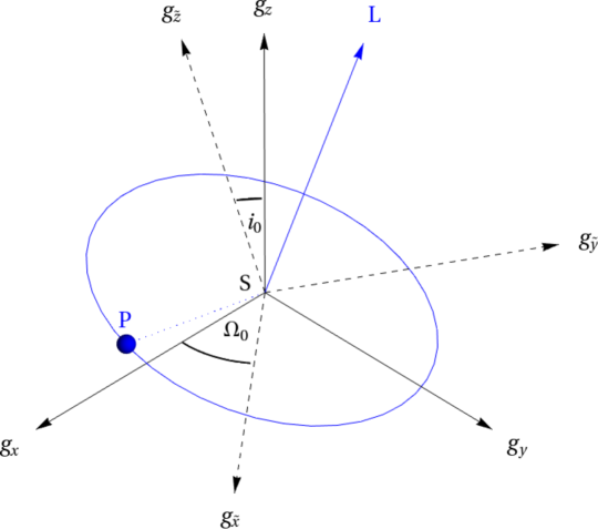
Figure 2: Heliocentric reference frames: ecliptic $(\vec{g}_{x},\vec{g}_{y},\vec{g}_{z})$ - thick, equatorial $(\vec{g}_{\tilde{x}},\vec{g}_{\tilde{y}},\vec{g}_{\tilde{z}})$ - dashed. The orbit frame is shown in blue with vector of angular momentum $\vec{L}$.

The heliocentric reference frame $\mathcal{G}_{Sun}=\{\vec{g}_{x},\vec{g}_{y},\vec{g}_{z}\}$ described above, we consider the heliocentric frames $\tilde{\mathcal{G}}_{Sun}=\{\vec{g}_{\tilde{x}},\vec{g}_{\tilde{y}},\vec{g}_{\tilde{z}}\}$ and $\tilde{\mathcal{G}}^{sc}_{Sun}=\{\vec{g}_{r},\vec{g}_{\theta},\vec{g}_{\phi}\}$ defined as follows: The unit vectors ($\vec{g}_{\tilde{x}}$, $\vec{g}_{\tilde{y}}$) span the Sun’s equatorial plane, with $\vec{g}_{\tilde{x}}$ directed along the line of intersection between the ecliptic and equatorial planes, and $\vec{g}_{\tilde{z}}$ is aligned with the rotation axis of the Sun. Then, the following relation holds

$$\vec{g}_{\tilde{x}} = \cos\left(\Omega_{0}\right)\vec{g}_{x}+\sin\left(\Omega_{0}\right)\vec{g}_{y}\ ,$$

$$\vec{g}_{\tilde{y}} = \cos\left(i_{0}\right)\left[-\sin\left(\Omega_{0}\right)\vec{g}_{x}+\cos\left(\Omega_{0}\right)\vec{g}_{y}\right]+\sin\left(i_{0}\right)\vec{g}_{z}\ ,$$

$$\vec{g}_{\tilde{z}} = \sin\left(i_{0}\right)\left[\sin\left(\Omega_{0}\right)\vec{g}_{x}-\cos\left(\Omega_{0}\right)\vec{g}_{y}\right]+\cos\left(i_{0}\right)\vec{g}_{z}\ ,$$ (8)

where $\Omega_{0}$ is the angle in the ecliptic plane between the direction of the vernal equinox and the line of nodes between the equatorial and ecliptic planes, and $i_{0}$ is the inclination of the Sun’s equator with respect to the ecliptic plane.

Let $(r,\theta,\phi)$ be the spherical coordinates in the equatorial system of reference, that is $r\geq 0$ is the radial distance, $0\leq\theta\leq\pi$ is the polar angle and $0\leq\phi<2\pi$ is the azimuthal angle. $\vec{g}_{r}$, $\vec{g}_{\theta}$, $\vec{g}_{\phi}$ are the local orthogonal unit vectors in the directions of increasing $r$, $\theta$ and $\phi$, respectively, defined as

$$\vec{g}_{r} = \sin\left(\theta\right)\left[\cos\left(\phi\right)\vec{g}_{\tilde{x}}+\sin\left(\phi\right)\vec{g}_{\tilde{y}}\right]+\cos\left(\theta\right)\vec{g}_{\tilde{z}}\ ,$$

$$\vec{g}_{\theta} = \cos\left(\theta\right)\left[\cos\left(\phi\right)\vec{g}_{\tilde{x}}+\sin\left(\phi\right)\vec{g}_{\tilde{y}}\right]-\sin\left(\theta\right)\vec{g}_{\tilde{z}}\ ,$$

$$\vec{g}_{\phi} = -\sin\left(\phi\right)\vec{g}_{\tilde{x}}+\cos\left(\phi\right)\vec{g}_{\tilde{y}}\ .$$ (9)

For later convenience, we also introduce a reference frame centered at the position of the dust grain, denoted by $\mathcal{G}^{RTN}_{Dust}=\{\vec{g}_{R},\vec{g}_{T},\vec{g}_{N}\}$. This orbital frame of reference is defined as follows. $\vec{g}_{R}=\vec{g}_{r}$ is directed along the radial vector that connects the origin (located in the center of the Sun) and the position of the dust grain. The unit vector $\vec{g}_{N}$ is aligned with the direction of the angular orbital momentum of the unperturbed dust grain, i.e. subject only to the gravitational attraction of the Sun. The right handed set is completed by means of the unit vector $\vec{g}_{T}$ oriented in the direction of the velocity vector of the grain. We note that this $RTN$ system is different from the $RTN$ system that has been defined in literature to implement the interplanetary magnetic field (see Horvath et al., 2006). In this study, the electromagnetic fields are solely referred in a $(r,\theta,\phi)$ system.

Let the angles $i$, $\omega$, $\Omega$, $f$ denote the inclination, argument of perihelion, longitude of the ascending node, and true anomaly of the dust grain orbit, defined with respect to the ecliptic system, respectively. We define the true longitude $u=\omega+f$ and we introduce the matrix

$${\mathbf{R}}={\mathbf{R}}_{3}\left(-u\right){\mathbf{R}}_{1}\left(-i\right){\mathbf{R}}_{3}\left(-\Omega\right)\ ,$$ (10)

where ${\mathbf{R}}_{j}(\psi)$ denotes the rotation matrix of angle $\psi$ around the axis $j$ with $j=1,3$, such that:

$${\mathbf{R}}_{1}\left(\psi\right) = \left(\begin{array}[]{ccc}1&0&0\\ 0&\cos(\psi)&-\sin(\psi)\\ 0&\sin(\psi)&\cos(\psi)\\ \end{array}\right)\ ,$$

$${\mathbf{R}}_{3}\left(\psi\right) = \left(\begin{array}[]{ccc}\cos(\psi)&-\sin(\psi)&0\\ \sin(\psi)&\cos(\psi)&0\\ 0&0&1\\ \end{array}\right)$$

Then, the components $F_{x}$, $F_{y}$, $F_{z}$ of the force $\vec{F}$, expressed in the reference frame $\mathcal{G}_{Sun}$, are transformed into the components $F_{R}$, $F_{T}$, $F_{N}$ in the orbital RTN system $\mathcal{G}^{RTN}_{Dust}=\{\vec{g}_{R},\vec{g}_{T},\vec{g}_{N}\}$ through the relation:

$$\left(F_{R},F_{T},F_{N}\right)^{T}={\mathbf{R}}\left(F_{x},F_{y},F_{z}\right)^{T}\ .$$ (13)

Parker spiral model.

In this paper, the interplanetary magnetic field is described by the Parker spiral model (Webb et al., 2010; Bieber et al., 1987), given as:

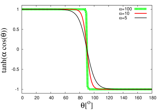
Figure 3: The function $\tanh(\alpha\cos(\theta))$ for various values of the parameter $\alpha$.

$$\vec{B}=\frac{Af\left(\theta\right)}{r^{2}}\left(\vec{g}_{r}-\frac{\Omega_{s}r\sin\left(\theta\right)}{u_{sw}}\vec{g}_{\phi}\right)\ ,$$ (14)

where the dimensional constant $A=B_{0}r_{0}^{2}$ is expressed in terms of the background magnetic field strength $B_{0}$, given at the reference distance $r_{0}$. The Lorentz force depends on the magnitude of the radial component of the solar wind speed $u_{sw}$, the solar rotation rate $\Omega_{s}$, and the sign change function $f(\theta)$, which defines the polarity of the magnetic field (magnetic north) of the Sun and can be given in terms of the Heaviside step function as $f(\theta)=1-2H(\theta-\pi/2)$. Thus, $f(\theta)$ is equal to $1$ above the equator ($\theta<\pi/2$) and $f(\theta)$ will change sign to $-1$ for $\theta>\pi/2$. We note that $f(\theta)$ can easily be modified to incorporate additional effects, like the sectorial structure of the interplanetary magnetic field.

Since $f(\theta)$ is discontinuous at $\theta=90^{o}$, we will replace this function by the smooth function $\tanh(\alpha\cos(\theta))$, where $\alpha$ is a positive parameter. Figure 3 shows that in simulations it is enough to consider $\alpha\geq 100$.

Denoting $\tilde{x}$, $\tilde{y}$ and $\tilde{z}$ the components of $\vec{r}$ in the frame $\tilde{\mathcal{G}}^{sc}_{Sun}$, that is we have $\tilde{x}=r\sin\theta\cos\phi$, $\tilde{y}=r\sin\theta\sin\phi$, $\tilde{z}=r\cos\theta$, it is easy to write the term $r\sin\theta\,\,\vec{g}_{\phi}$, appearing in (14), in the form

$$r\sin\theta\,{\vec{g}}_{\phi}=-\tilde{y}{\vec{g}}_{\phi}+\tilde{x}{\vec{g}}_{\phi}={\vec{g}}_{\tilde{z}}\times{\vec{r}}\ .$$ (15)

Moreover, from the first equation of $\eqref{e:s2e}$ we obtain

$$\cos\theta=\frac{{\vec{r}}\cdot{\vec{g}}_{\tilde{z}}}{r}\ .$$ (16)

Therefore, by using the relations (15) and (16), the relation (14) can be rewritten in the form

$$\vec{B}=\frac{B_{0}r_{0}^{2}}{r^{2}}\left(\frac{\vec{r}}{r}-\frac{\Omega_{s}}{u_{sw}}{\vec{g}}_{\tilde{z}}\times{\vec{r}}\right)\tanh\Bigl{(}\alpha\frac{{\vec{r}}\cdot{\vec{g}}_{\tilde{z}}}{r}\Bigr{)}\ .$$ (17)

Combining (6), (7) and (17), we obtain that the Lorentz force ${\vec{F}}_{L}$ has the form:

$${\vec{F}}_{L}=-\frac{qB_{0}r_{0}^{2}}{r^{2}}\Bigl{[}{\frac{1}{r}\,\vec{r}}\times\dot{\vec{r}}+\frac{\Omega_{s}}{r}{\vec{r}}\times({\vec{r}}\times{\vec{g}}_{\tilde{z}})+\frac{\Omega_{s}}{u_{sw}}({\vec{r}}\times{\vec{g}}_{\tilde{z}})\times\dot{\vec{r}}\Bigr{]}\tanh\Bigl{(}\alpha\frac{{\vec{r}}\cdot{\vec{g}}_{\tilde{z}}}{r}\Bigr{)}$$ (18)

where ${\vec{g}}_{\tilde{z}}$ is given by the third relation of $\eqref{e:ec2eq}$.

Remark 1

Lorentz force defined by (18) is conservative, that is there exists the function

$$\Upsilon(\vec{r})=-\frac{qB_{0}r_{0}^{2}\Omega_{s}}{\alpha}\ln\Bigr{[}\cosh\Bigl{(}\alpha\frac{{\vec{r}}\cdot{\vec{g}}_{\tilde{z}}}{r}\Bigr{)}\Bigr{]}\ ,$$ (19)

such that

$${\vec{F}}_{L}\cdot d{\vec{r}}=-d\Upsilon.$$

Indeed, from (18) we deduce

$${\vec{F}}_{L}\cdot d{\vec{r}}=-\frac{qB_{0}r_{0}^{2}\Omega_{s}}{r^{3}}\Bigl{[}({\vec{r}}\cdot{\vec{g}}_{\tilde{z}})\,({\vec{r}}\cdot d{\vec{r}})-r^{2}({\vec{g}}_{\tilde{z}}\cdot d{\vec{r}})\Bigr{]}\tanh\Bigl{(}\alpha\frac{{\vec{r}}\cdot{\vec{g}}_{\tilde{z}}}{r}\Bigr{)}$$

$$=qB_{0}r_{0}^{2}\Omega_{s}\tanh\Bigl{(}\alpha\frac{{\vec{r}}\cdot{\vec{g}}_{\tilde{z}}}{r}\Bigr{)}\,d\Bigl{(}\frac{{\vec{r}}\cdot{\vec{g}}_{\tilde{z}}}{r}\Bigr{)}=-d\Upsilon.$$

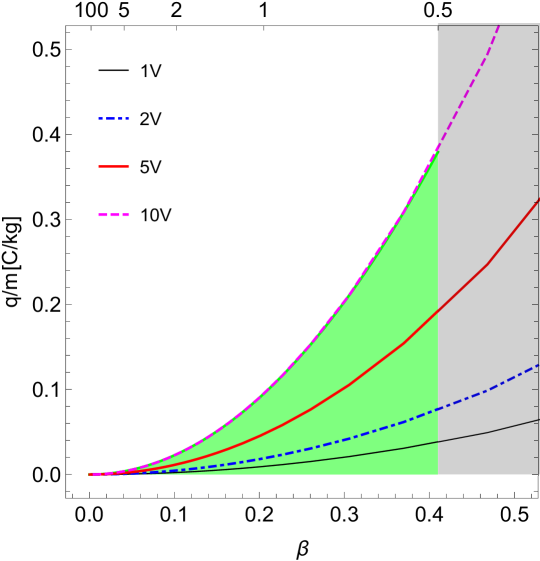
Figure 4: Region of interest (light green) in the space $(\beta,\gamma)$. Numbers at the top correspond to $R$ in $\mu m$.

Choice of parameters.

As described above, equation of motion (1), i.e. (2)–(7), depends on the following parameters: the ratio $q/m$ between the charge and mass of the dust grain, the ratio $\beta$ between the magnitudes of the forces due to solar radiation pressure and the gravitational attraction of the Sun, the ratio $\eta$ of the magnitudes of the forces due to the solar wind and the Poynting-Robertson effect, the spectrally averaged efficiency factor $Q$ and the solar wind speed $u_{sw}$. Following Lhotka et al. (2016); Kocifaj et al. (2006), in this paper we consider the following parameters as fixed constants: $\eta=1/3$, $Q=1$ and $u_{sw}=400\,[km/s]$.

Parameters $\beta$ and $q/m$ are related to other physical parameters of the problem. Let the density and radius of the dust grain be parameterized by $\rho$, and $R$, respectively. We assume that the dust grain is of spherical shape, and has constant density and radius. Under this assumption the mass of the grain is simply given by the formula $m=4\pi/3\rho R^{3}$. On the other hand, the charge $q$ of the dust grain is related to $U$, the surface electric potential of the grain, by the formula: $q=4\pi\varepsilon_{0}\,U\,R$, where $\varepsilon_{0}$ denotes the dielectric constant in vacuum. Assuming perfectly absorbing dust particles (Beauge and Ferraz-Mello, 1994) and setting $\rho=2.8\,[g/cm^{3}]$, we obtain approximate formulas that are sufficient for the purpose of our study:

$$\beta=0.205/R\quad\gamma=0.0094U/R^{2}\ .$$ (20)

Here, $\gamma$ is the numerical value of $q/m$ expressed in $[C/kg]$ ($q/m=\gamma[C/kg]$), the particle radius $R$ is given in microns and the surface potential $U$ in Volts. Thus, the dimensionless quantities $(\beta,\gamma)$ are given in terms of $(R,U)$ (and vice versa). Table 1 gives various quantities and numerical values that we use in our study.

Table 1: Parameters that we use in our study. ^(a) taken from NASA planetary fact sheet https://nssdc.gsfc.nasa.gov/planetary/factsheet/. ^(b) calculated from $\rho$, $U$, $R$. ^(c) obtained from $i_{0}$, $\Omega_{0}$.

symbol	values	reference
$a_{1}$	$a_{J}$	(a)
$\alpha$	$100$	this work
$B_{0}$	3nT	Meyer-Vernet (2012)
$\beta$	0…0.5	Beauge and Ferraz-Mello (1994)
$c$	299792458km/s	Stöcker (2014)
$\varepsilon_{0}$	$8.854187\times 10^{-12}F/m$	Stöcker (2014)
$\eta$	$1/3$	Klačka (2014)
$\gamma$	$0\dots 0.5C/kg$	(b)
$i_{0}$	$7.15^{o}$	Beck and Giles (2005)
$m_{0}$	$M_{\odot}$	(a)
$m$	$4\pi/3\rho R^{3}$	Stöcker (2014)
$m_{1}$	$m_{J}$	(a)
$r_{0}$	$1AU$	Meyer-Vernet (2012)
$r_{1}$	$a_{1}$	(a)
$\Omega_{0}$	$73.5^{o}$	Beck and Giles (2005)
$\Omega_{s}^{-1}$	$24.47d$	Meyer-Vernet (2012)
$Q$	$1$	Beauge and Ferraz-Mello (1994)
$R$	$0\dots 500\mu m$	Gruen et al. (1994)
$\rho$	$2.8g/cm^{3}$	Beauge and Ferraz-Mello (1994)
$u_{sw}$	400km/s	Meyer-Vernet (2012)
$U$	$0\dots 10V$	Mann et al. (2014)
$x_{0},y_{0},z_{0}$	$(0.12,0.04,0.99)$	(c)

To ensure the dominant term in (1) is due to solar gravity only, we limit the region of interest of our study in the space $(\beta,\gamma)$ as shown in light green in Fig. 4. The dark shaded rectangle marks regions in $(\beta,\gamma)$ where central gravity is less than twice the force due to solar radiation pressure (see top of Fig. 1).

Choice of initial conditions.

In this study we are interested in the behaviour of the orbital elements of the charged particle in the vicinity of outer $p+q:p$ mean-motion resonances with Jupiter, where the effect of radiation pressure on the mean-motion of the dust particle, see (5), is taken into account. The value of the semi-major axis of the dust particle at exact resonance is given by the relation (equation 16 in Beauge and Ferraz-Mello, 1994):

$$a_{p+q:p}=\left(\frac{p}{p+q}\right)^{2/3}a_{1}\left(1-\beta\right)^{1/3}$$

which follows from

$$n^{2}a^{3}=\mu(1-\beta)\quad n_{1}^{2}a_{1}^{3}=\mu\ ,$$

and using the relation $n:n_{1}=p+q:p$. Here, $a_{1}$, $n_{1}$ denote the semi-major axis and mean-motion of Jupiter. Let $\lambda=M+\omega+\Omega$, $\lambda_{1}=M_{1}$ denote the orbital longitudes of the dust particle and Jupiter, respectively (in agreement with the choice of reference frame such that the argument of perihelion and longitude of the ascending node of Jupiter vanish). The resonant angular argument $s$ at $p+q:p$ resonance is thus given by (Beauge, 1994; Beauge and Ferraz-Mello, 1994):

$$qs=(p+q)\lambda_{1}-p\lambda-q\bar{\omega}\ ,$$

where we used the notation $\bar{\omega}=\omega+\Omega$.

3 Isolated influence of the interplanetary magnetic field

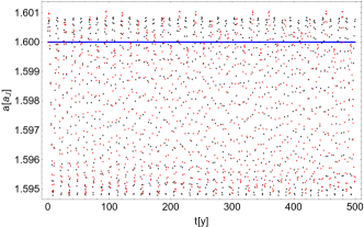
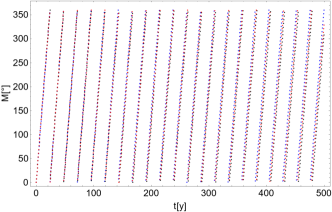
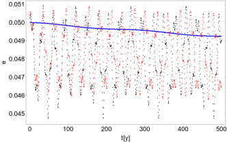
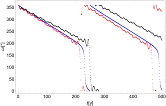
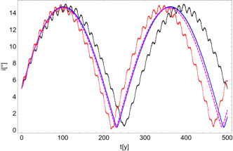
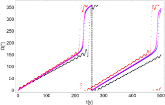
Figure 5: Orbit for $a(0)=1.6a_{J}$, $e(0)=0.05$, $i(0)=5^{o}$, and $\Omega(0)=\omega(0)=M(0)=0$. Comparison of Cartesian model (black), Gauss model (red), and averaged Gauss model (blue). The dominant dynamics takes place in the $(\Omega,i)$-plane. The magenta (dashed) line is the solution obtained from (3), the vertical dashed line in the lower right figure is calculated from the period of (27).

In this section we derive an analytical model that takes into account the influence of the Keplerian part (5) and the Lorentz force (18). The aim of such a simplified model is to understand the orbital evolution of a charged dust particle subject to the polarity change of the Sun’s magnetic field in the long-term. The information provided by such a toy model is relevant in the study of the full model that also takes into account the influence of Jupiter, the Poynting-Robertson effect and solar wind drag. The analytical results are used in Section 4 to describe the complex phenomena arising in the neighbourhood of outer resonances with Jupiter.

The procedure for deriving this toy model is presented in detail in Lhotka et al. (2016). Since this uses averaging theory, we underline the fact that the analytical results will only be valid on the average over one orbital period of the charged dust particle, and under the assumption that the eccentricities are small, the inclinations have moderate values, and the deviations of the magnetic axis from the angular momentum axis of the system are also small. Our approach differs from Lhotka et al. (2016) as follows: 1) we allow the magnetic axis of the magnetic field to be misaligned with the angular momentum vector of the Kepler problem. 2) In the present study we also include a sign change function unlike our approach in Lhotka et al. (2016).

Our results in this section are based on the simplified dynamical problem:

$$m\vec{\ddot{r}}={\vec{F}}_{Kep}+{\vec{F}}_{L}\ ,$$ (21)

with ${\vec{F}}_{Kep}$ given by (5) and ${\vec{F}}_{L}$ given by (18). The Lorentz force is not affected by the position of Jupiter. The perturbation due to the planet is thus not taken into account in the present discussion. Without loss of generality, we set $\beta=0$ in (5). First we derive Gauss’ planetary equations of motion (see, e.g. Fitzpatrick, 2012) on the basis of (21):

$$\frac{d{\vec{O}}}{dt}={\vec{G}}\left(\vec{O}\right),$$ (22)

with $\vec{O}=\left(a,e,i,\omega,\Omega,M\right)$, and $\vec{G}$ is used to denote the vector field that enters Gauss’ planetary equations. Starting from (18) we first express $r$, $\vec{r}$, $\dot{\vec{r}}$ in terms of series expansions of the orbital elements by making use of Bessel functions (see, e.g. Dvorak and Lhotka, 2013). The force ${\vec{F}}_{L}$ depends on the hyperbolic tangent of the term ${\vec{r}}\cdot{\vec{g}}_{\tilde{z}}/r$ that corresponds to $(xx_{0}+yy_{0}+zz_{0})/r$ with $x_{0}=\sin\Omega_{0}\sin i_{0}$, $y_{0}=-\sin i_{0}\cos\Omega_{0}$, $z_{0}=\cos i_{0}$, and $x$, $y$, $z$ are the components of $\vec{r}$ in the frame $\mathcal{G}_{Sun}$. We make use of Lambert’s continued fraction representation of the function $\tanh$: to zeroth order in eccentricity $e$, and for $x_{0},y_{0}<<1$, $z_{0}\sim 1$ we find:

$$\frac{\tanh\Bigl{(}\alpha\frac{{\vec{r}}\cdot{\vec{g}}_{\tilde{z}}}{r}\Bigr{)}}{\alpha} \simeq \cos(\Omega)\left(x_{0}\cos(M+\omega)+y_{0}\cos(i)\sin(M+\omega)\right)-$$ (23)

$$\sin(\Omega)\left(x_{0}\cos(i)\sin(M+\omega)-y_{0}\cos(M+\omega)\right)+$$

$$z_{0}\sin(i)\sin(M+\omega)\ .$$

We note that (23) is valid for small deviations of the magnetic axis from the inertial $z$-axis, for small eccentricities, and moderate inclinations. Further calculations to obtain Gauss’ planetary equations in the form (22) are straightforward (see, e.g. Lhotka et al., 2016) and have been implemented using specialized computer algebra routines in Wolfram Mathematica. In the following exposition we mainly address the secular contributions of the dynamics that are obtained by averaging $\vec{G}$ over one orbital period of the dust grain expanded up to first order in $x_{0}$, $y_{0}$, $1-z_{0}$, and vanishing $e$. As numerical simulations show (e.g. Kocifaj et al., 2006), the mean effect of the Lorentz force mainly affects the orientation of the orbital planes of the dust particles. In this section we confirm this result by analysis of the averaged equations of motions. The averaged parts of the force system $F_{R}$, $F_{T}$, $F_{N}$ in (13) and (22) reduce to a non-vanishing normal component equal to:

$${\bar{F}}_{N} \simeq -\alpha\frac{3}{2}\frac{q}{m}B_{0}r_{0}^{2}\mu^{1/2}\frac{e}{a^{5/2}}\big{\{}\cos(\omega)\big{[}x_{0}\cos(\Omega)+y_{0}\sin(\Omega)\big{]}+$$ (24)

$$\sin(\omega)\big{[}\cos(i)\left(y_{0}\cos(\Omega)-x_{0}\sin(\Omega)\right)+z_{0}\sin(i)\big{]}\big{\}}\ .$$

Since the averages of $\bar{F}_{R}$, $\bar{F}_{T}$ are zero we conclude that the secular effects due to the interplanetary magnetic field mainly act on inclination $i$ and on the ascending node $\Omega$, while the Lorentz force does not alter the remaining Kepler elements on secular time scales. Ignoring the short-periodic effects, we therefore fix the orbital elements $a$, $e$, and investigate the dynamics in the phase plane ($i$, $\Omega$). The components $i$ and $\Omega$ in Gauss’ planetary equations of motions are given by (see, e.g. Fitzpatrick, 2012):

$$\frac{di}{dt} = \frac{\cos\left(u\right)rF_{N}}{na^{2}\left(1-e^{2}\right)^{1/2}},\$$

$$\frac{d\Omega}{dt} = \frac{\sin\left(u\right)rF_{N}}{na^{2}\left(1-e^{2}\right)^{1/2}\sin\left(i\right)}\ .$$ (25)

To first order in $x_{0}$, $y_{0}$, $1-z_{0}$, and vanishing $e$, the secular part that enters (22), (3) reduces to:

$$\frac{di}{dt} \simeq -\alpha\frac{q}{m}\frac{B_{0}}{2}\left(\frac{r_{0}}{a}\right)^{2}\bigg{\{}\left[1-\cos\left(i\right)z_{0}\frac{\Omega_{s}}{n}\right]\times\bigg{(}x_{0}\cos\left(\Omega\right)+y_{0}\sin\left(\Omega\right)\bigg{)}\bigg{\}},\$$

$$\frac{d\Omega}{dt} \simeq -\alpha\frac{q}{m}\frac{B_{0}}{2}\left(\frac{r_{0}}{a}\right)^{2}\bigg{\{}\left[\cot\left(i\right)-z_{0}\frac{\cos\left(2i\right)}{\sin\left(i\right)}\frac{\Omega_{s}}{n}\right]\times$$ (26)

$$\bigg{(}y_{0}\cos\left(\Omega\right)-x_{0}\sin\left(\Omega\right)\bigg{)}+\cos\left(i\right)\left(1-2z_{0}\right)\frac{\Omega_{s}}{n}+z_{0}\bigg{\}}\ .$$

We conclude that variations in inclinations and the ascending node are proportional to the charge-to-mass ratio $q/m=\gamma[C/kg]$, the background magnetic field strength $B_{0}$, and the square of the inverse distance of the dust grain from the Sun $1/a^{2}$. Variations in inclinations are furthermore amplified by the magnitudes of $x_{0}$ and $y_{0}$, proportional to a common proportionality factor $1-\cos\left(i\right)z_{0}\Omega_{s}/n$. The dominant frequency term in the second equation in (3) depends on $\cos\left(i\right)$, the ratio $\Omega_{s}/n$, and $z_{0}$, which is the cosine of $i_{0}$. We conclude that the overall effect of the perturbations due to the interplanetary magnetic field (in absence of a normal magnetic field component, see Lhotka et al., 2016) on the orbital plane of a charged dust particle mainly depends on the actual value of $i_{0}$, inclination $i$, and the ratio $\Omega_{s}/n$. Let

$$\Gamma=\alpha\frac{q}{m}\frac{B_{0}}{2}\left(\frac{r_{0}}{a}\right)^{2}\ .$$

In the limit $x_{0},y_{0}\to 0$ and $z_{0}\to 1$, for fixed values of the semi-major axis $a$, and inclination $i$, the solution for the ascending node becomes:

$$\Omega(t)=\left(\cos\left(i\right)\frac{\Omega_{s}}{n}-1\right)\Gamma t+\Omega(0)\ .$$ (27)

Thus, for fixed $\Gamma$ the period of the ascending node decreases for larger values of inclination $i$, and increases for larger values of $\Omega_{s}/n$. Next, we aim to solve (3) in the limit $\Omega_{s}/n\to 0$, which minimizes the period of the ascending node. Assuming small inclination $i$, we introduce the non-singular and non-canonical variables:

$$p = \tan\left(i\right)\sin\left(\Omega\right)$$

$$q = \tan\left(i\right)\cos\left(\Omega\right)\ ,$$ (28)

which transforms (3) up to $O(p,q)$:

$$\frac{dp}{dt}=-\Gamma\left(y_{0}+z_{0}q\right)\ ,\frac{dq}{dt}=-\Gamma\left(x_{0}-z_{0}p\right)\ ,$$ (29)

The linearised system has the solution:

$$p(t)\simeq\frac{\left(p_{0}z_{0}-x_{0}\right)\cos\left(z_{0}\Gamma t\right)-\left(q_{0}z_{0}+y_{0}\right)\sin\left(z_{0}\Gamma t\right)+x_{0}}{z_{0}}\ ,$$

$$q(t)\simeq\frac{\left(p_{0}z_{0}-x_{0}\right)\sin\left(z_{0}\Gamma t\right)+\left(q_{0}z_{0}+y_{0}\right)\cos\left(z_{0}\Gamma t\right)-y_{0}}{z_{0}}\ .$$ (30)

From the solution it follows that the motion in the $(p,q)$-plane takes place along a circle with radius $(x_{0}+y_{0}+q_{0}z_{0})/z_{0}$ (with $q(0)=\tan\left(i(0)\right)$ and $p(0)=0$), centered around $(x_{0},-y_{0})$. We note that the estimates are based on averaged and linearised equations that are only valid for $x_{0},y_{0}<<1$, $z_{0}\simeq 1$, vanishing eccentricities, small inclinations, and in the limit $\Omega_{s}/n\to 0$. To demonstrate the validity of the analytical results of the current section we show a specific orbit in Fig. 5. The full, unaveraged solution obtained from (21) is shown in black, the unaveraged solution obtained from (22) is shown in red. The solution is well approximated with the fully averaged model obtained from (22), and the numerical solution of the reduced dynamical system (3), which is shown in magenta. We note that the estimate of the period of $\Omega$ obtained from (27), indicated by the dashed vertical line at the bottom right of Fig. 5, is in perfect agreement with the numerical solution of the problem. However, the simplified solution given by (27) is unable to reproduce the complex evolution in time of the ascending node longitude since it is lacking of higher order terms in its derivation. We also show the same orbit projected on the phase-plane $(p,q)$ in Fig. 6. The unaveraged solution based on (21) is shown in black, the averaged solution based on (3) in magenta. The analytical solution (3) is indicated by the green line, and is confirmed by the dashed circle with center and radius based on the considerations above.

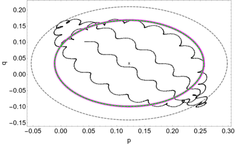
Figure 6: Orbit of Fig. 5 projected to the $(p,q)$-plane. See text.

We conclude that the dynamics in the $(i,\Omega)$-plane of charged dust in the heliosphere is dominated by the deviation of the magnetic and orbital angular momentum axis and the rotation period of the Sun. In our simplified model the motion is regular and follows invariant curves in the $(p,q)$-plane. We note that the rotation period in the $(p,q)$ plane, and thus the frequency of $\Omega$ strongly depend on the choice for $\alpha$ that is present in the formulae due to the approximation of the $\tanh$ in (18). For the presentation of the results a reasonable choice of $\alpha$ has been made to show the agreement between the averaged and unaveraged equations of motion. For different values of $\alpha$ the frequencies may be over- or underestimated.

4 Numerical study of the full problem

In this section we perform several numerical experiments in order to highlight the role of the Lorentz force on the long-term evolution of the orbital elements of a charged dust grain located in the vicinity of outer mean-motion resonances with Jupiter. By merging arguments given by analytical theories with numerical investigations, in the following section we unveil a rich dynamical behavior in the vicinity of resonance consisting of chaotic motions, trapped motions, temporary captures, escapes from resonance, jumps, etc. Such phenomena are highly influenced, or rather induced, by the complex interactions between the Lorentz force and the other perturbations. For the purpose of exposition we focus on the neighborhood of the 1:2 mean-motion resonance only. While only specific test cases are shown to demonstrate various effects, many numerical simulations have been performed to come to our conclusions. Similar results are found close to the 1:3 and 2:3 mean-motion resonances. A complete survey of the parameter and initial condition space for different resonances will be the subject of a subsequent paper.

The dynamics of exterior mean-motion resonances has been studied in detail in several works, such as Message (1958); Sicardy et al. (1993); Lazzaro et al. (1994); Beauge (1994); Beauge and Ferraz-Mello (1994), within both the conservative planar circular restricted three body problem and the framework of the dissipative model that includes, in addition, the influence of the Poynting-Robertson effect. These studies have revealed a plethora of interesting dynamical features of outer mean-motion resonances (as compared with interior resonances) for example: the existence of asymmetric libration regions, namely regions in which the resonant angle does not librate around zero or $\pi$, temporary captures into resonances due to Poynting-Robertson drag, the existence of a so-called universal eccentricity - that is an eccentricity towards which all librational orbits will evolve regardless the values of the drag coefficient or the planetary mass, etc.

Before describing the dynamical phenomena due to the Lorentz force and the combined influence of the Lorentz force and dissipative effects, let us recall first the structure of the phase portrait of the 1:2 resonance. We disregard for the moment the influence of the Lorentz force, Poynting-Robertson effect and solar wind drag - that is we consider, as a starting point of discussion, the restricted three body problem (the model that takes into account the effects of ${\vec{F}}_{Kep}$ and ${\vec{F}}_{Jup}$) and we focus on the case of 1:2 resonance, located at $a_{1:2}=2^{2/3}a_{1}\,(1-\beta)^{1/3}$ (Beauge and Ferraz-Mello, 1994).

The dynamics of exterior mean-motion resonances, within the context of planar restricted problem of three bodies, has been investigated in Beauge (1994) by using the Hamiltonian formalism. Starting from a two-degrees-of-freedom non-autonomous Hamiltonian and assuming that the system lies in the vicinity of an exterior mean-motion resonance, the problem was reduced, by averaging the Hamiltonian with respect to the synodic period, to a single-degree-of-freedom problem characterized by a Hamiltonian depending on the action $J=L-G$, where $L$ and $G$ are the well-known Delaunay variables, the critical angle $s$ and an external parameter $N$ that is a constant of motion within the averaged problem (see Beauge, 1994). For the resonance considered here, $N$ has the expression

$$N=\sqrt{\mu(1-\beta)a}\,\Bigl{(}2\sqrt{1-e^{2}}-1\Bigr{)}.$$ (31)

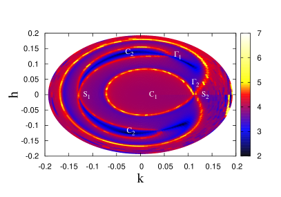
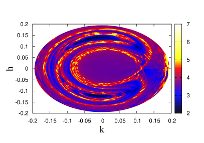
Figure 7: FLI map for 1:2 resonance at $N=1.155$ with $i(0)=0^{o}.1$, $\omega(0)=0^{o}$, $\Omega(0)=0^{o}$, $\beta=0.1$, $\gamma=0$ (left) and $\gamma=0.00227$ (right). Parameters correspond to particles with diameter $R=2\,[\mu m]$ and $1\,[V]$ surface charge.

Left panel of Figure 7 shows the phase portrait of the 1:2 resonance, within the context of the model defined by ${\vec{F}}_{Kep}$, ${\vec{F}}_{Jup}$ and the conservative part in (3). Results are shown in the non-canonical variables $(k,h)=(e\cos(s),e\sin(s))$, for $N=1.155$, in units of $\mu=1$, $a_{1}=1$ (see, Beauge, 1994). Using Cartesian equations of motion and plotting the Fast Lyapunov Indicator, hereafter denoted by FLI (Froeschlé et al., 1997; Guzzo et al., 2002; Guzzo and Lega, 2013), we numerically recover the dynamical features of the 1:2 resonance, described in Beauge (1994) by using analytical arguments related to single-degree-of-freedom Hamiltonians. Indeed, FLI reveals after a short computational time the entire topological structure of the phase space. Namely: two asymmetric libration regions (dark blue) with the centers $C_{2}$ situated at $s\simeq\pm 95^{o}$, two separatrices $\Gamma_{1}$ and $\Gamma_{2}$ (yellow lines) associated with the saddle points $S_{1}$ and $S_{2}$ respectively, an inner circulation region (dark-red) with the center $C_{1}$, and the outer circulation region. The separatrix $\Gamma_{1}$ surrounds the two asymmetric libration regions, while $\Gamma_{2}$ splits the $(k,h)$ plane into the inner circulation region, the libration zone (i.e. with orbits along which the critical angle $s$ does not take all values between $0^{o}$ and $360^{o}$) and the outer circulation region. The libration zone includes the two asymmetric libration regions and the region bounded by $\Gamma_{1}$ and $\Gamma_{2}$, which contain the orbits exhibiting large-amplitude librations around the unstable point $S_{1}$.

Within the dynamical background described above, let us now consider the effects induced by the Lorentz force (18). In this section, we consider a fixed value of the parameter $\beta=0.1$, which correspond to a sample object having the size $R=2[\mu m]$, provided the density is $\rho=2.8[g/cm^{3}]$, and let the parameter $\gamma$ vary. The right panel of Figure 7 was obtained under the same conditions as the left panel, but now the Lorentz force was ”switched on”. We note that even if the parameter $q/m=\gamma[C/kg]$ is small (namely the numerical value $\gamma=0.00227$, corresponding to just $1\,[V]$ surface charge), the FLI map shows several yellow regions that infer the onset of chaotic motions. Indeed, the color scale in Figure 7 provides a measure of the FLI, which gives an indication of the regular or chaotic dynamics: small values (i.e., dark colors) correspond to regular motions, while larger values (i.e., red to yellow colors) denote chaotic regions. The yellow regions suggest the appearance of chaotic motions, that is some orbits might pass in an unpredictable way from the libration regime to the circulation regime, or from small-amplitude librations around one of the centers $C_{2}$ to large-amplitude librations around the saddle point $S_{1}$ and vice versa.

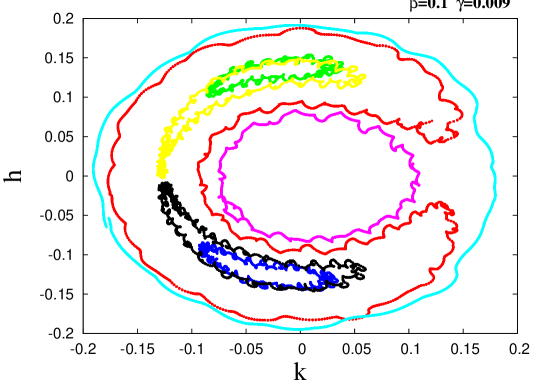
Figure 8: Phase portrait for the 1:2 resonance, for $N=1.155$ in units of $\mu=1$, $a_{1}=1$ (see the text), under the effect of the following perturbations: Jupiter, the conservative part of the solar radiation pressure and Lorentz force. Parameters $\beta=0.1$ and $\gamma=0.009$ correspond to particles with diameter $R=2\,[\mu m]$ and $4\,[V]$ surface charge. The osculating initial conditions of the seven orbits are $i(0)=0^{o}.1$, $\omega(0)=0^{o}$, $\Omega(0)=0^{o}$ and: $e=0.14$, $s=30^{o}$ (red), $e=0.139$, $s=80^{o}$ (green), $e=0.124$, $s=276^{o}$ (blue), $e=0.08$, $s=200^{o}$ (pink), $e=0.19$, $s=200^{o}$ (light blue), $e=0.13$, $s=186^{o}$ (yellow), $e=0.13$, $s=188^{o}$ (black).

Since chaos occurs for rather small values of $\gamma$, one may ask whether librational motions are still possible for larger values of this parameter. The question is also motivated by the analytical results described in the previous section showing that the Lorentz force induces a large-amplitude variation of inclination, up to $10$ degrees (see e.g. Figure 5), which is not present for $q=0$. The answer is provided by Figure  8, obtained for the value of $\gamma$ that corresponds to $4[V]$ surface charge. This Figure shows that in the $(k,h)$ plane all the motions described within the framework of the planar restricted three body problem are possible. However, this plot was obtained by propagating seven orbits for a relatively short period of time on the order of hundreds of years. Depending on initial conditions and the parameter $\gamma$, on a longer time scale the perturbations due to the Lorentz force lead to chaotic variations of the orbital elements.

Figure 9: Variation of semimajor axis $a$, resonant angle $s$, eccentricity $e$ and inclination $i$ for an orbit inside the 1:2 resonant regime. The parameters and osculating initial conditions are: $N=1.155$, $\beta=0.1$, $q/m=0.009[C/kg]$, $e=0.14$, $s=72.5^{o}$, $i(0)=0^{o}.1$, $\omega(0)=0^{o}$ and $\Omega(0)=0^{o}$.

Figure 9 depicts a trapping trajectory into the resonance for more than $45\,[ky]$. We remark that the initial conditions are close to the green orbit of Figure 8. Left panels show the evolution of semi-major axis and eccentricity, while the right panels describe the behavior of the resonant angle $s$ and the inclination $i$. The resonance does not affect the evolution of inclination, which varies periodically due to the Lorentz force (see the previous section); the right bottom plot of Figure 9 shows the variation of inclination over 5$\,[ky]$. One particular phenomenon revealed by the top right panel of Figure 9 is the jump from one type of librational motion to another and vice versa. Thus, as an effect of the Lorentz force, this particular orbit exhibits short-amplitude librations around either the center situated at $s\simeq 95^{o}$, or the stable point located at $s\simeq-95^{o}$, and even large-amplitude librations around the saddle point $S_{1}$. Of course, the jumps are unpredictable, and a small change in the initial conditions leads to a different dynamical behavior.

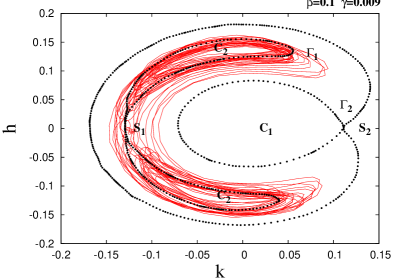
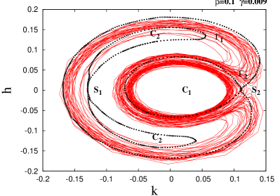
Figure 10: Trapped motion into 1:2 resonance (left) and escape motion from it (right), under the same effects as in Figure 9. Left panel: variation of the $(k,h)$ variables for the orbit shown in Figure 9. Right panel: the orbit characterized by the following parameters and initial conditions: $N=1.155$ in units of $\mu=1$, $a_{1}=1$, $\beta=0.1$, $q/m=0.009[C/kg]$, $e=0.16$, $s=180^{o}$, $i(0)=0^{o}.1$, $\omega(0)=0^{o}$ and $\Omega(0)=0^{o}$.

The left panel of Figure 10 shows the evolution in the $(k,h)$ plane of the orbit presented in Figure 9. To highlight various dynamical behaviors, in particular the jumps from one libration region to another, on the background of Figure 10 we draw the separatrices $\Gamma_{1}$ and $\Gamma_{2}$ from the planar restricted three body model. In the right panel of Figure 10 we present another dynamical behavior due to the Lorentz force, that is the escape from the libration region of the 1:2 resonance. Indeed, this panel shows an orbit initially exhibiting large-amplitude librations around the unstable point $S_{1}$, namely in the libration region bounded by $\Gamma_{1}$ and $\Gamma_{2}$, but due to the perturbations it crosses the separatrix and reaches into the inner circulation region.

The figures described above are obtained within the conservative framework (with all forces except (3)), and provide an image of the dynamical behavior inside the resonance (Figures 9 and 10). Let us consider now the full dynamical model characterized by equation (1) and analyze the orbital evolution of non-resonant initial conditions. Within the dissipative regime it is well known (Sicardy et al., 1993) that Poynting-Robertson effect leads to temporary capture into exterior resonances, a dynamical mechanism that was analyzed in Beauge and Ferraz-Mello (1994) by applying the adiabatic invariant theory. Moreover, it has been shown (Sicardy et al., 1993; Lazzaro et al., 1994; Beauge and Ferraz-Mello, 1994) that there exists a so-called universal eccentricity towards which all librational orbits will evolve regardless of the values of the drag coefficient or the planetary mass. The question we address here is the following: how does the Lorentz force (18) influence the process of capture into resonance? All numerical simulations suggest that the Lorentz force does not influence the capture process itself; all non-resonant initial conditions placed at a longer distance from the Sun than the location of resonance evolve to a librational orbit. However, the resulted trapped motions are shorter than in the absence of the Lorentz force. Depending on the initial conditions and the value of $\gamma$, the orbits could be trapped in resonance from $10^{4}$ to $10^{6}$ years. Figure 11 reports some results obtained by propagating three orbits having the same initial conditions and the same parameters, but $q/m$ set to $\gamma=0$ (red), $\gamma=0.015$ (green) and $\gamma=0.022$ (blue). The values $\gamma=0.015$ (green) and $\gamma=0.022$ (blue) correspond to large surface charges of $6.6\,[V]$ and $9.7\,[V]$, respectively. These examples show that even for large magnitudes of the Lorentz force the capture mechanism is not affected. For the orbit in blue both the capture and escape phenomena are clearly depicted by the bottom left panel of Figure 11. The orbit in green is captured into resonance for more than 450 years. We also note that orbits can be captured in any of the two asymmetric libration regions. As a final remark, the top right panel of Figure 11 provides a numerical evidence that also in this case there exists an universal eccentricity; eccentricities of the orbits trapped in resonance evolve toward a value independently from the rest of the orbital elements, in particular the inclination, and independent of the perturbations.

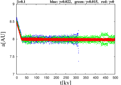
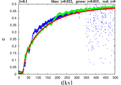
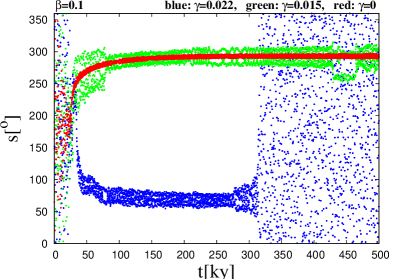
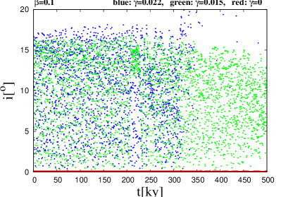
Figure 11: Capture into the 1:2 resonance and escape from it. Variation of the semimajor axis $a$, resonant angle $s$, eccentricity $e$ and inclination $i$ for three orbits. The orbits in green and blue are obtained under the perturbing effects of the attraction of Jupiter, solar radiation pressure, Poynting-Robertson drag and Lorentz force, while the orbit drawn in red was obtained under the influence of Jupiter, solar radiation pressure and Poynting-Robertson drag. The parameters and osculating initial conditions are: $N=1.155$, $\beta=0.1$, $e(0)=0.001$, $s(0)=0^{o}$, $i(0)=0^{o}.1$, $\omega(0)=50^{o}$, $\Omega(0)=15^{o}$ and respectively $q/m=0.022[C/kg]$ (blue), $q/m=0.015[C/kg]$ (green) and $q/m=0$ (red). The values $\gamma=0.022$ ($\gamma=0.015$) correspond to about $9.7\,[V]$ ($6.6\,[V]$) surface charge.

Finally, we perform numerical simulations in the full parameter space (green in Fig. 4) on the grid $(\beta,\gamma)$ using discrete steps of $0.005$ in $\beta$ and $0.001$ in $\gamma$. We start the dust grain on a circular orbit within the orbital plane of Jupiter at the distance $a(0)=8.326AU$ and $M(0)=0$. We investigate the time for which the orbit of a charged grain stays in the vicinity of the outer 1:2 resonance of the uncharged problem. For this reason we define the region $D_{1:2}$ as follows. The semi-major axis of the uncharged dust grain shrinks until the particle is trapped at resonance. Let $D_{1:2}$ be the interval $(0.95a_{min},1.05a_{max})$ within the time interval $(0,100ky)$ of the orbit of the uncharged particle. Here, $a_{min}$ and $a_{max}$ are the minimum and maximum values of $a(t)$ during the time of integration equal to $T=100ky$ of the uncharged grain. For the charged particles we determine the first moment in time, say $T_{s}$ when the semi-major axis of the charged grain lies outside of $D_{1:2}$. We then calculate the ratio $T_{s}/T$ for each set of parameters $(\beta,\gamma)$, that is, the time for which the orbit of the charged particle stays in the vicinity of the uncharged problem. We note that the ratio does not imply that the orbit of the charged particle is always trapped in resonance. However, it serves as a rough measure for the stability in semi-major axis $a$. The results are summarized in Fig. 12. Black dots indicate pairs of $(\beta,\gamma)$ for which $T_{s}/T=1$ and white dots indicate $T_{s}/T=0$, while intermediate cases are shown in gray. The figure clearly demonstrates that in the majority of the cases, the time of temporary capture is decreased when including the effects of the Lorentz force due to the interaction of charged particles with the interplanetary magnetic field.

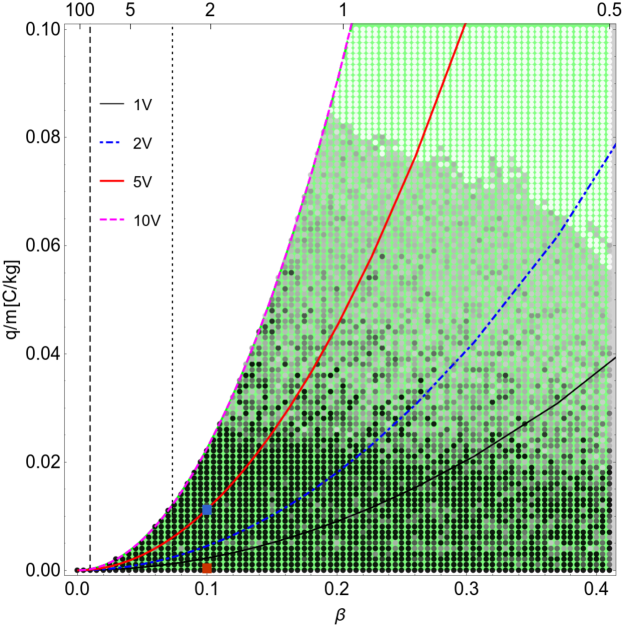
Figure 12: Magnification of Fig. 4. Dots label the parameters $\beta,q/m=\gamma[C/kg]$ that have been used in our study. The color code indicates how long the dust grain stays within the vicinity of the 1:2 resonance compared to the orbit with $\gamma=0$ (black = 100%, white = 0%).

We note that in Fig. 11 inclinations vary with amplitudes around $15^{o}$ for $\gamma\neq 0$. The effect on the inclination stems from the Lorentz force due to the interaction with the interplanetary magnetic field (see model (3) obtained in Section 3). For $\gamma=0$, variations in inclinations vanish, which can also be observed in the full model (see case red in Fig. 11). To investigate the effect of $\gamma$ on the orbital parameters, we look for the maximum values of $e$ and $i$ during their evolution in time. The results are summarized in Figure 13, where we show $\max(e)$ and $\max(i)$ for the same simulation data as in Fig. 12. The black region in Fig. 12 corresponds to the orange (dark gray) region in Fig. 13. Within this region, eccentricities are bound within ($0\leq e\leq 0.7$) and inclinations stay within the interval ($0\leq i\leq 30^{o}$) throughout the numerical integrations. Outside this region eccentricities may reach $e=1$ (white dots) and values beyond (blank) in Fig. 12, while inclinations are found up to values about $i\simeq 180^{o}$. As a direct consequence, the possibility of collisions and close encounters of the dust particle with planet Jupiter is increased, which will lead to reduced times in temporary capture in comparison to the uncharged problem. We notice, that the gray and white regions in Fig. 12 cannot be seen in Fig. 13. The light gray region in Fig. 12 indicates the range of parameters $\beta$ and $\gamma$ for which the dust grains are captured - about half the capture time of the uncharged dust grains with equivalent diameters. In this region, release from resonance occurs due to an increase of orbital parameters $e$ and $i$ somewhere in the middle of the orbital evolution, but the maximum values that have been calculated to produce Fig. 13 show values stemming from the second half of the orbital evolution of the dust grain orbits. The same arguments hold true in the white region of Fig. 12. The mechanism for the reduction of temporary capture of dust grain orbits in mean-motion resonance with Jupiter can be explained by the enlargement of the chaotic regimes close to resonance (see Fig. 7). As a result, the time of temporary capture in resonance is decreased - charged dust particles in the solar system are less stable than neutral ones.

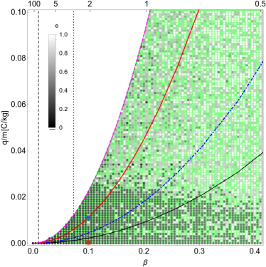
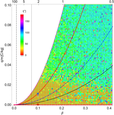
Figure 13: Maximum values of $e$ (left) and $i$ (right) in the parameter plane $\beta,q/m=\gamma[C/kg]$. Color code of lines correpsonds to the color code of Fig. 12. Within the orange (gray) region variations in inclinations are less than $30^{o}$.

5 Summary of the results and discussion

In this work we investigated the effect of the Lorentz force due to the heliospheric magnetic field on the orbits of charged, micron-sized dust grains in the vicinity of outer mean-motion resonances with Jupiter with special focus on the 1:2 resonance. We confirm previous results based on the assumption of uncharged particles with some minor modifications. Our main results can be summarized as follows:

• The effect of the Lorentz force strongly affects the orbital planes of the dust grains. Therefore, the problem cannot be understood within the framework of the planar problem. We extend the problem to the spatial case, and find by means of averaging theory the amplitudes of variations in orbital inclinations of dust grains orbits. Moreover, the orbital planes experience a drift in ascending node longitudes on secular time scales. The effect on inclinations is related to the angle between the angular momentum and magnetic axes of the problem and the rotation rate of the Sun, see the discussion of (3) in Section 3.

• No major effect of the interplanetary magnetic field on the capture mechanism in outer mean-motion resonances could be found. The capture process is dominated by solar wind drag and the Poynting-Robertson effect like for uncharged particles. The transient time (before capture) turns out to be the same for charged and uncharged particles, see the discussion of Figure 11 in Section 4.

• Resonant motion is present for charged dust grains like already found for uncharged particles. However, the effect of the Lorentz force induces additional perturbations that lead to complex dynamical phenomena. Most notably we find jumps of the resonant argument from one libration center to the other, and separatrix crossings (see the discussions in Section 4).

• The presence of the interplanetary magnetic field affects the capture process. The existence of the Lorentz force makes some dynamical processes faster, i.e. escape from the resonant region (see, e.g. Figure 11).

This work is the second in a series of papers devoted to the dynamics of charged, micron-sized dust grains in the heliosphere (see also Lhotka et al., 2016). A detailed survey of the parameter space for different outer mean-motion resonances is going to be finalized in the near future and should include more sophisticated models of the interplanetary magnetic field.

Acknowledgements This work is supported by the Austrian Science Fund (FWF) with project number P-30542. CG was supported by a grant of the Romanian National Authority for Scientific Research and Innovation, CNCS-UEFISCDI, project number PN-III-P1-1.1-TE-2016-2314. We thank the members of the Space Plasma Group at the Space Research Institute of the Austrian Academy of Science for useful discussions about modelling the interplanetary magnetic field.

The authors declare that they have no conflict of interest.

References

- Froeschlé et al. [1997] C. Froeschlé, E. Lega, and R. Gonczi. Fast Lyapunov Indicators. Application to asteroidal motion. Celestial Mechanics and Dynamical Astronomy, 67(1):41–62, January 1997. ISSN 1572-9478. doi: 10.1023/A:1008276418601.
- Guzzo and Lega [2013] M. Guzzo and E. Lega. The numerical detection of the Arnold web and its use for long-term diffusion studies in conservative and weakly dissipative systems. Chaos, 23(1):023124, June 2013. doi: 10.1063/1.4807097.
- Guzzo et al. [2002] M. Guzzo, E. Lega, and Froeschlé. On the numerical detection of the effective stability of chaotic motions in quasi-integrable systems. Physica D: Nonlinear Phenomena, 163(1):1–25, March 2002. doi: 10.1016/S0167-2789(01)00383-9.
- Beauge [1994] C. Beauge. Asymmetric liberations in exterior resonances. Celestial Mechanics and Dynamical Astronomy, 60:225–248, October 1994. doi: 10.1007/BF00693323.