Linear Constrained Rayleigh Quotient Optimization:
Theory and Algorithms

Abstract

We consider the following constrained Rayleigh quotient optimization problem (CRQopt)

$$\min_{x\in\mathbb{R}^{n}}x^{\operatorname{T}}Ax\,\,\mbox{subject to}\,\,x^{\operatorname{T}}x=1\,\mbox{and}\,C^{\operatorname{T}}x=b,$$

where $A$ is an $n\times n$ real symmetric matrix and $C$ is an $n\times m$ real matrix. Usually, $m\ll n$. The problem is also known as the constrained eigenvalue problem in the literature because it becomes an eigenvalue problem if the linear constraint $C^{\operatorname{T}}x=b$ is removed. We start by equivalently transforming CRQopt into an optimization problem, called LGopt, of minimizing the Lagrangian multiplier of CRQopt, and then an problem, called QEPmin, of finding the smallest eigenvalue of a quadratic eigenvalue problem. Although such equivalences has been discussed in the literature, it appears to be the first time that these equivalences are rigorously justified. Then we propose to numerically solve LGopt and QEPmin by the Krylov subspace projection method via the Lanczos process. The basic idea, as the Lanczos method for the symmetric eigenvalue problem, is to first reduce LGopt and QEPmin by projecting them onto Krylov subspaces to yield problems of the same types but of much smaller sizes, and then solve the reduced problems by some direct methods, which is either a secular equation solver (in the case of LGopt) or an eigensolver (in the case of QEPmin). The resulting algorithm is called the Lanczos algorithm. We perform convergence analysis for the proposed method and obtain error bounds. The sharpness of the error bound is demonstrated by artificial examples, although in applications the method often converges much faster than the bounds suggest. Finally, we apply the Lanczos algorithm to semi-supervised learning in the context of constrained clustering.

1 Introduction

In this paper, we are concerned with the following linear constrained Rayleigh quotient (CRQ) optimization:

$$\min~{} v^{\operatorname{T}}Av,$$ (1.1a)

s.t. $$v^{\operatorname{T}}v=1,$$ (1.1b)

$$C^{\operatorname{T}}v=b,$$ (1.1c)

where $A\in\mathbb{R}^{n\times n}$ is symmetric, i.e., $A=A^{\operatorname{T}}$, $C\in\mathbb{R}^{n\times m}$ has full column rank, and $b\in\mathbb{R}^{m}$. Necessarily $m<n$ but often $m\ll n$. We are particularly interested in the case where $A$ is large and sparse and $b\neq 0$.

CRQopt (1.1) is also known as the constrained eigenvalue problem, a term coined in [10] in 1989. However, it had appeared in the literature much earlier than that [15]. In that sense, it is a classical problem. However, past studies are fragmented with some claims, although often true, not rigorously justified or needed conditions to hold. In this paper, our goal is to provide a thorough investigation into this classical problem, including rigorous justifications of statements previously taken for granted in the literature and addressing the theoretical subtleties that were not paid attention to. We also present a quantitative convergence analysis for the Krylov type subspace projection method, which we will also call the Lanczos algorithm, for solving large scale CRQopt (1.1).

Related works.

CRQopt (1.1) has found a wide range of applications, such as ridge regression [5, 12], trust-region subproblem [27, 33], constrained least square problem [9], spectral image segmentation [6, 36], transductive learning [19], and community detection [28].

The first systematic study of CRQopt (1.1) perhaps belongs to Gander, Golub and von Matt [10]. Using the full QR and eigen-decompositions, they first reformulated CRQopt (1.1) as an optimization problem of finding the minimal Lagrangian multiplier via solving a secular equation (in a way that is different from our secular equation solver in Appendix A). Alternatively, they also turned CRQopt (1.1) into an optimization problem of finding the smallest real eigenvalue of a quadratic eigenvalue problem (QEP). However, the equivalence between the QEP optimization and the Lagrangian multiplier problem was not rigorously justified there.

Numerical algorithms proposed in [10] are not suitable for large scale CRQopt (1.1) because they requires a full eigen-decomposition of $A$ as a dense matrix. Later in [14], Golub, Zhang and Zha considered large and sparse CRQopt (1.1) but only with the homogeneous constraint, i.e, $b=0$. In this special case, CRQopt (1.1) is equivalent to computing the smallest eigenvalue of $A$ restricted to the null space of $C^{\operatorname{T}}$. An inner-outer iterative Lanczos method was proposed to solve the homogeneous CRQopt (1.1). In [41], Xu, Li and Schuurmans proposed a projected power method for solving CRQopt (1.1). The projected power method is an iterative method only involving matrix-vector products, and thus it is suitable for large and sparse CRQopt (1.1). However, its convergence is linear at best and often too slow. In [6], Eriksson, Olsson and Kahl reformulated CRQopt (1.1) into an eigenvalue optimization problem (see Appendix B for details) An algorithm based on the line search was used to find the optimal solution. This algorithm is suitable for CRQopt (1.1) with a large and sparse matrix $A$, but it is too costly because the smallest eigenvalue has to be computed multiple times during each line search action.

Contributions.

Our study in this paper on CRQopt (1.1) begins with the standard approach of Lagrangian multipliers, as was taken in [10], which leads to an optimization problem of minimizing the Lagrangian multiplier of CRQopt, called LGopt (Section 2.2), and then an optimization problem of finding the smallest real eigenvalue of a quadratic eigenvalue problem (QEP), called QEPmin (Section 2.3). We summarize our major contributions as follows.

1. Although transforming CRQopt into LGopt and QEPmin is not really new, our formulations of LGopt and QEPmin set them up onto a natural path for use in Krylov subspace type projection methods that only requires matrix-vector products. Therefore, the formulations are suitable for large scale CRQopt. We rigorously proved the equivalences among the three problems while they were only loosely argued previously as, e.g., in [10]. As far as subtle technicalities are concerned, we prove that the leftmost eigenvalue in the complex plane is real, which has a significant implication when it comes to numerical computations.

2. We devise a Lanczos algorithm to solve the induced optimization problems: LGopt and QEPmin. This algorithm is made possible, as we argued moments ago, by our different formulations from what in the literature. Along the way, we also propose an efficient numerical algorithm for the type of secular equations arising from solving each projected LGopt.

3. We establish a quantitative convergence analysis for the Lanczos algorithm and obtain error bounds on approximations generated by the algorithm. These error bounds are in general sharp in the worst case as demonstrated by artificially designed numerical examples.

4. We apply our algorithm to the large scale CRQopt from the constrained clustering that arises from the standard spectral algorithm with linear constraints to encode prior knowledge labels. During our tests, we observed that our algorithm was $2$ to $23$ times faster than FAST-GE-2.0 [18] for constrained image segmentation, depending on given image data.

Organization.

In Section 2, we investigate the theoretical aspect of CRQopt (1.1) such as the feasible set, the existence of a minimizer, and transforming CRQopt (1.1) into two equivalent optimization problems with rigorous justifications. A Krylov subspace projection approach for solving CRQopt (1.1) via its equivalent optimization problems just mentioned are detailed in Section 3 and its convergence analysis is given in Section 4. Numerical examples that demonstrate the sharpness of our error bounds for convergence are presented in Section 5. Section 6 describes an application of our algorithms to the constrained image segmentation problem. Concluding remarks are in Section 7. There are three appendices. Appendix A explains how to solve the secular equation arising from solving the reduced LGopt. Appendix B proves the equivalence between CRQopt (1.1) and an eigenvalue optimization problem proposed by Eriksson, Olsson and Kahl [6]. Appendix C documents CRQPACK, a software package for an implementation of Lanczos algorithm and reproducing numerical experiments presented in this paper.

Notation.

Throughout the article, $\mathbb{R}$, $\mathbb{R}^{n}$ and $\mathbb{R}^{m\times n}$ are set of real numbers, columns vectors of dimension $n$, and $m\times n$ matrices, respectively. $\mathbb{C}$, $\mathbb{C}^{n}$ and $\mathbb{C}^{m\times n}$ are set of complex numbers, columns vectors of dimension $n$, and $m\times n$ matrices, respectively. We use MATLAB-like notation $X_{(i:j,k:l)}$ to denote the submatrix of $X$, consisting of the intersections of rows $i$ to $j$ and columns $k$ to $l$, and when $i:j$ is replaced by $:$, it means all rows, similarly for columns. For a vector $v\in\mathbb{C}$, $v_{(k)}$ refers the $k$th entry of $v$ and $v_{(i:j)}$ is the subvector of $v$ consisting of the $i$th to $j$th entries inclusive. The $n\times n$ identity matrix is $I_{n}$ or simply $I$ if its size is clear from the context, and $e_{j}$ is the $j$th column of an identity matrix whose size is determined by the context. $\operatorname{diag}(c_{1},c_{2},\dots,c_{n})$ is an $n\times n$ diagonal matrix with diagonal elements $c_{1},c_{2},\dots,c_{n}$. The imaginary unit is $\mbox{\tt i}=\sqrt{-1}$.

For $X\in\mathbb{C}^{m\times n}$, $X^{\operatorname{T}}$, ${\cal R}(X)$, ${\cal N}(X)$ denote its transpose, range and null space, respectively. For a real symmetric matrix $H$, $\operatorname{eig}(H)$ stands for the set of all eigenvalues of $H$, and $\lambda_{\min}(H)$ and $\lambda_{\max}(H)$ denote the smallest and largest eigenvalue of $H$, respectively. $\|\cdot\|_{p}$ $(1\leq p\leq\infty$) is the $\ell_{p}$-vector or $\ell_{p}$-operator norm, respectively, depending on the argument. As a special case, $\|\cdot\|_{2}$ or $\|\cdot\|$ is either the Euclidean norm of vector or the spectral norm of a matrix.

2 Theory

2.1 Feasible set and solution existence

In CRQopt (1.1), we assumed $\operatorname{rank}(C)=m$. Let

$$n_{0}=(C^{\operatorname{T}})^{{\dagger}}b,$$ (2.1)

i.e., $n_{0}$ is the unique minimal norm solution of $C^{\operatorname{T}}v=b$, where $C^{{\dagger}}$ is the Moore-Penrose inverse of $C$. Because of the assumption $\operatorname{rank}(C)=m$, we have [1, 4, 38]

$$C^{{\dagger}}=(C^{\operatorname{T}}C)^{-1}C^{\operatorname{T}},\,\,(C^{\operatorname{T}})^{{\dagger}}=(C^{{\dagger}})^{\operatorname{T}}=C(C^{\operatorname{T}}C)^{-1}.$$

The most important orthogonal projection throughout this article is

$$P=I-CC^{{\dagger}}$$ (2.2)

which orthogonally projects any vector onto ${\cal N}(C^{\operatorname{T}})$, the null space of $C^{\operatorname{T}}$ [38]. Any $v\in\mathbb{R}^{n}$ that satisfies $C^{\operatorname{T}}v=b$ can be orthogonally decomposed as

$$v=(I-P)v+Pv=n_{0}+Pv\in n_{0}+{\cal N}(C^{\operatorname{T}}).$$ (2.3)

Evidently $\|v\|^{2}=\|n_{0}\|^{2}+\|Pv\|^{2}$, which, together with the unit length constraint (1.1b), lead to the following immediate conclusions about the solvability of CRQopt (1.1):

• If $\|n_{0}\|>1$, then there is no unit vector $v$ satisfying $C^{\operatorname{T}}v=b$. This is because for any $v$ satisfying $C^{\operatorname{T}}v=b$ has norm no smaller than $\|n_{0}\|$. Thus CRQopt (1.1) has no minimizer.

• If $\|n_{0}\|=1$, then $v=n_{0}$ is the only unit vector that satisfies $C^{\operatorname{T}}v=b$. Thus CRQopt (1.1) has a unique minimizer $v=n_{0}$.

• If $\|n_{0}\|<1$, then there are infinitely many feasible vectors $v$ that satisfy $C^{\operatorname{T}}v=b$.

Therefore only the case $\|n_{0}\|<1$ needs further investigation. Consequently, throughout the rest of the article, we will assume $\|n_{0}\|<1$.

2.2 Equivalent LGopt

Using the orthogonal decomposition (2.3), we have

$$v^{\operatorname{T}}Av =v^{\operatorname{T}}PAPv+2v^{\operatorname{T}}PAn_{0}+n_{0}^{\operatorname{T}}An_{0},$$ (2.4a)

$$v^{\operatorname{T}}v =\|n_{0}\|^{2}+\|Pv\|^{2}.$$ (2.4b)

Since $n_{0}^{\operatorname{T}}An_{0}$ and $\|n_{0}\|$ are constants, CRQopt (1.1) is equivalent to the following constrained quadratic minimization problem

$$\min~{} v^{\operatorname{T}}PAPv+2v^{\operatorname{T}}b_{0},$$ (2.5a)

s.t. $$\|Pv\|=\gamma,$$ (2.5b)

$$v\in n_{0}+{\cal N}(C^{\operatorname{T}}),$$ (2.5c)

where

$$b_{0}=PAn_{0}\in{\cal N}(C^{\operatorname{T}}),\quad\gamma:=\sqrt{1-\|n_{0}\|^{2}}>0.$$ (2.6)

Necessarily, $0<\gamma<1$. However, in the rest of our development, unless we refer back to CRQopt (1.1), $\gamma<1$ can be removed, i.e., $\gamma$ can be any positive number.

Theorem 2.1.

$v_{\ast}$ is a minimizer of CRQopt (1.1) if and only if $v_{\ast}$ is a minimizer of CQopt (2.5).

One way to solve CQopt (2.5) is the method of the Lagrangian multipliers. It seeks the stationary points of the Lagrangian function

$$\mathscr{L}(v,\lambda)=v^{\operatorname{T}}PAPv+2v^{\operatorname{T}}b_{0}-\lambda(v^{\operatorname{T}}Pv-\gamma^{2}).$$ (2.7)

Differentiating $\mathscr{L}$ with respect to $v$ and $\lambda$, we get

$$(PA-\lambda I)Pv =-b_{0},$$ (2.8a)

$$\|Pv\| =\gamma.$$ (2.8b)

Let $u=Pv\in{\cal N}(C^{\operatorname{T}})$. Then $u=Pu$ and $v=n_{0}+u$. The Lagrangian equations in (2.8) are equivalent to the following equations:

$$(PAP-\lambda I)u =-b_{0},$$ (2.9a)

$$\|u\| =\gamma,$$ (2.9b)

$$u \in{\cal N}(C^{\operatorname{T}}).$$ (2.9c)

In fact, any solution $(\lambda,v)$ of (2.8) gives rise to a solution $(\lambda,u)$ with $u=Pv$ of (2.9), and conversely any solution $(\lambda,u)$ of (2.9) leads to a solution $(\lambda,v)$ with $v=n_{0}+u$ of (2.8).

The system of equations (2.9) has more than one solution pairs $(\lambda,u)$. We seek a pair $(\lambda,u)$ among them that minimizes the objective function of (2.5) for $v\in\mathbb{R}^{n}$. Note that

$$f(v): =v^{\operatorname{T}}PAPv+2v^{\operatorname{T}}b_{0}$$

$$=v^{\operatorname{T}}PAPv+2v^{\operatorname{T}}PAn_{0}$$

$$\stackrel{{\scriptstyle\text{$u=Pv$}}}{{=}}u^{\operatorname{T}}Au+2u^{\operatorname{T}}An_{0}$$

$$\stackrel{{\scriptstyle\text{$u=Pu$}}}{{=}}u^{\operatorname{T}}PAPu+2u^{\operatorname{T}}PAn_{0}$$

$$=u^{\operatorname{T}}PAPu+2u^{\operatorname{T}}b_{0}$$

$$=f(u),$$ (2.10)

i.e., $f(v)=f(u)$ for $v\in\mathbb{R}^{n}$ and $u=Pv$. Therefore minimizing $f(v)$ over $v\in\mathbb{R}^{n}$ is equivalent to minimizing $f(u)$ over $u\in{\cal N}(C^{\operatorname{T}})$. The following lemma compares the value of $f$ at different solution pairs $(\lambda,u)$ of the system (2.9). The proof of the lemma is inspired by Gander [9] on solving a least squares problem with a quadratic constraint,

Lemma 2.1.

For two solution pairs $(\lambda_{i},u_{i})$ for $i=1,2$ of the Lagrangian system of equations (2.9), $\lambda_{1}<\lambda_{2}$ if and only if $f(u_{1})<f(u_{2})$.

Proof.

The proof relies on the following three facts:

1. For any solution pair $(\lambda,u)$ of (2.9), we have

   $$\lambda u=PAPu+b_{0}\quad\Rightarrow\quad\lambda=\frac{1}{u^{\operatorname{T}}u}{u^{\operatorname{T}}(PAPu+b_{0})}=\frac{1}{\gamma^{2}}{u^{\operatorname{T}}(PAPu+b_{0})}.$$ (2.11)

2. Given $(\lambda_{i},u_{i})$ for $i=1,2$, satisfying (2.9), we have

   $$f(u_{1}) =u_{1}^{\operatorname{T}}PAPu_{1}+2u^{\operatorname{T}}_{1}b_{0}$$

   $$\stackrel{{\scriptstyle\text{ \eqref{eq:CQopt-LagEq'-1}}}}{{=}}-b^{\operatorname{T}}_{0}u_{1}+\lambda_{1}u_{1}^{\operatorname{T}}u_{1}+2u^{\operatorname{T}}_{1}b_{0}$$

   $$\stackrel{{\scriptstyle\text{ \eqref{eq:CQopt-LagEq'-2}}}}{{=}}u^{\operatorname{T}}_{1}b_{0}+\lambda_{1}\gamma^{2}$$

   $$\stackrel{{\scriptstyle\text{ \eqref{eq:CQopt-LagEq'-1}}}}{{=}}-u_{2}^{\operatorname{T}}(PAP-\lambda_{2}I)u_{1}+\lambda_{1}\gamma^{2}.$$

   Similarly, we have $f(u_{2})=-u_{1}^{\operatorname{T}}(PAP-\lambda_{1}I)u_{2}+\lambda_{2}\gamma^{2}$. Therefore

   $$f(u_{1})-f(u_{2})=(\lambda_{1}-\lambda_{2})(\gamma^{2}-u_{1}^{\operatorname{T}}u_{2}).$$ (2.12)

3. For $u_{i}$ of norm $\gamma$, by the Cauchy-Schwartz inequality, $u_{1}^{\operatorname{T}}u_{2}\leq\|u_{1}\|\,\|u_{2}\|=\gamma^{2}$, and $u_{1}^{\operatorname{T}}u_{2}=\|u_{1}\|\,\|u_{2}\|=\gamma^{2}$ if and only if $u_{1}=u_{2}$. Hence if $u_{1}\neq u_{2}$, then $\gamma^{2}-u_{1}^{\operatorname{T}}u_{2}>0$.

Now we are ready to prove the claim of the lemma. If $\lambda_{1}<\lambda_{2}$, then $u_{1}\neq u_{2}$ otherwise (2.11) would imply $\lambda_{1}=\lambda_{2}$, and thus $f(u_{1})<f(u_{2})$ by (2.12). On the other hand, if $f(u_{1})<f(u_{2})$, then $\gamma^{2}-u_{1}^{\operatorname{T}}u_{2}>0$ because $\gamma^{2}-u_{1}^{\operatorname{T}}u_{2}\geq 0$ always and it cannot be $0$ by (2.12), and thus $\lambda_{1}-\lambda_{2}<0$ again by (2.12). ∎

As a consequence of Lemma 2.1, we find that solving CQopt (2.5) is equivalent to solving the smallest Lagrangian multiplier $\lambda$ of (2.7), i.e., those $\lambda$ that satisfy (2.9). Specifically, solving CQopt (2.5) is equivalent to solving the following Lagrangian minimization problem:

$$\min~{} \lambda$$ (2.13a)

s.t. $$(PAP-\lambda I)u=-b_{0},$$ (2.13b)

$$\|u\|=\gamma,$$ (2.13c)

$$u\in{\cal N}(C^{\operatorname{T}}).$$ (2.13d)

Theorem 2.2.

If $v_{\ast}$ is a minimizer of CQopt (2.5), then $(\lambda_{*},u_{*})$ with

$$u_{*}=Pv_{*},\,\,\lambda_{*}=\frac{1}{\gamma^{2}}{u_{*}^{\operatorname{T}}(PAPu_{*}+b_{0})}$$

is a minimizer of LGopt (2.13). Conversely if $(\lambda_{*},u_{*})$ is a minimizer of LGopt (2.13), then $v_{\ast}=n_{0}+u_{\ast}$ is a minimizer of CQopt (2.5).

The case $b_{0}=PAn_{0}=0$, which includes but is not equivalent to the homogeneous CRQopt (1.1) (i.e., $b=0$) [15, 14], can be dealt with as follows. Suppose $b_{0}=0$ and let $\theta_{1}$ be the smallest eigenvalue of $PAP$. Keep in mind that $PAP$ always has an eigenvalue $0$ with multiplicity $m$ associated with the subspace ${\cal N}(C^{\operatorname{T}})^{\bot}={\cal R}(C)$, the column space of $C$. There are the following two subcases:

• Subcase $\theta_{1}\neq 0$: Then $\theta_{1}<0$. Let $z_{1}$ be a corresponding eigenvector of $PAP$. Then $z_{1}=PAPz_{1}/\theta_{1}\in{\cal N}(C^{\operatorname{T}})$. So $(\theta_{1},z_{1})$ is a minimizer of LGopt (2.13) and therefore $z_{1}$ is a minimizer of CQopt (2.5), which in turn implies that $v_{\ast}=n_{0}+\gamma z_{1}/\|z_{1}\|$ is a minimizer of CRQopt (1.1).

• Subcase $\theta_{1}=0$: If there exists a corresponding eigenvector $z_{1}\in{\cal N}(C^{\operatorname{T}})$, i.e., $Pz_{1}\neq 0$, then $(\theta_{1},Pz_{1})$ is a minimizer of LGopt (2.13) and therefore $Pz_{1}$ is a minimizer of CQopt (2.5), which in turn implies that $v_{\ast}=n_{0}+\gamma Pz_{1}/\|Pz_{1}\|$ is a minimizer of CRQopt (1.1). Otherwise there exists no corresponding eigenvector $z_{1}$ such that $Pz_{1}\neq 0$. Let $\theta_{2}$ be the second smallest eigenvalue of $PAP$, which is nonzero, and $z_{2}$ a corresponding eigenvector. Then $z_{2}=PAPz_{2}/\theta_{2}\in{\cal N}(C^{\operatorname{T}})$, and $(\theta_{2},z_{2})$ is a minimizer of LGopt (2.13) and therefore $z_{2}$ is a minimizer of CQopt (2.5), which in turn implies that $v_{\ast}=n_{0}+\gamma z_{2}/\|z_{2}\|$ is a minimizer of CRQopt (1.1).

In view of such a quick resolution for the case $b_{0}=0$, in the rest of this article, we will assume

$$b_{0}=PAn_{0}\neq 0.$$ (2.14)

2.3 Equivalent QEPmin

Let $(\lambda,u)$ be a feasible pair of LGopt (2.13) and $\lambda\not\in\operatorname{eig}(PAP)$. We can write $u=-(PAP-\lambda I)^{-1}b_{0}$, and then

$$\gamma^{2}=u^{\operatorname{T}}u=b_{0}^{\operatorname{T}}(PAP-\lambda I)^{-2}b_{0}=b_{0}^{\operatorname{T}}z,$$ (2.15)

where $z=(PAP-\lambda I)^{-2}b_{0}$, or equivalently, $(PAP-\lambda I)^{2}z=b_{0}$. Therefore $b_{0}^{\operatorname{T}}z/\gamma^{2}=1$ by (2.15), and thus the pair $(\lambda,z)$ satisfies the quadratic eigenvalue problem (QEP):

$$(PAP-\lambda I)^{2}z=b_{0}=b_{0}\cdot 1=b_{0}\left(b_{0}^{\operatorname{T}}z/\gamma^{2}\right)=\frac{1}{\gamma^{2}}b_{0}b_{0}^{\operatorname{T}}z.$$ (2.16)

We claim that any $z$ satisfying (2.16) is in ${\cal N}(C^{\operatorname{T}})$. To see this, we expand $(PAP-\lambda I)^{2}z$ and extract $\lambda^{2}z$ from $(PAP-\lambda I)^{2}z=b_{0}$ to get

$$z=\frac{1}{\lambda^{2}}\left[-(PAP)^{2}z+2\lambda\cdot PAPz+b_{0}\right]\in{\cal N}(C^{\operatorname{T}}),$$

where we have used the assumption $\lambda\not\in\operatorname{eig}(PAP)$ to conclude $\lambda\neq 0$, and $b_{0}=PAn_{0}\in{\cal N}(C^{\operatorname{T}})$. Therefore we have shown that under the assumption that LGopt (2.13) has no feasible pair $(\lambda,u)$ with $\lambda\in\operatorname{eig}(PAP)$, any feasible pair $(\lambda,u)$ of LGopt (2.13) satisfies QEP (2.16) with $z\in{\cal N}(C^{\operatorname{T}})$.

Next, we prove that any pair $(\lambda,z)$ satisfying

$$0\neq z\in{\cal N}(C^{\operatorname{T}}),\,\,\lambda\not\in\operatorname{eig}(PAP)\,\,\mbox{and QEP \eqref{eq:QEP-deriv}},$$ (2.17)

leads to a feasible pair of the Lagrange equations (2.13). First we note that $b_{0}^{\operatorname{T}}z\neq 0$; otherwise we would have $(PAP-\lambda I)^{2}z=0$ by (2.16), implying $z=0$ since $\lambda\not\in\operatorname{eig}(PAP)$, a contradiction. Let $(\lambda,z)$ be a scalar-vector pair that satisfying (2.17). Define $u:=-(PAP-\lambda I)^{-1}b_{0}$. Then $(PAP-\lambda I)u=-b_{0}$, i.e., (2.13b) holds, and also

$$\lambda u=PAPu+b_{0}\quad\Rightarrow\quad u=\frac{1}{\lambda}(PAPu+b_{0})\in{\cal N}(C^{\operatorname{T}}),$$

i.e., (2.13d) holds. Without loss of generality, we may scale $z$ such that $b_{0}^{\operatorname{T}}z=\gamma^{2}$. It follows from (2.16) that

$$(PAP-\lambda I)^{2}z=b_{0}\quad\Rightarrow\quad z=(PAP-\lambda I)^{-2}b_{0},$$

implying

$$1=\frac{1}{\gamma^{2}}b_{0}^{\operatorname{T}}z=\frac{1}{\gamma^{2}}b_{0}^{\operatorname{T}}(PAP-\lambda I)^{-2}b_{0}=\frac{1}{\gamma^{2}}u^{\operatorname{T}}u\quad\Rightarrow\quad\|u\|=\gamma,$$

i.e., (2.13c) holds. Lemma 2.2 summarizes what we have just proved.

Lemma 2.2.

Suppose the constraints of LGopt (2.13) has no feasible pair $(\lambda,u)$ with $\lambda\in\operatorname{eig}(PAP)$, and suppose that QEP (2.16) has no solution pair $(\lambda,z)$ with $0\neq z\in{\cal N}(C^{\operatorname{T}})$ and $\lambda\in\operatorname{eig}(PAP)$. Then any pair $(\lambda,u)$ satisfying the constraints of LGopt (2.13) gives rise to a pair $(\lambda,z)$ with $z=(PAP-\lambda I)^{-2}b_{0}$ that satisfies QEP (2.16). Conversely, any pair $(\lambda,z)$ with $z\neq 0$ satisfying QEP (2.16) leads to a pair $(\lambda,u)$ with $u:=-(PAP-\lambda I)^{-1}b_{0}$ that satisfies the constraints of LGopt (2.13).

As a corollary of Lemma 2.2, we conclude that LGopt (2.13) is equivalent to

$$\min~{} \lambda$$ (2.18a)

s.t. $$(PAP-\lambda I)^{2}z=\gamma^{-2}b_{0}b_{0}^{\operatorname{T}}z,$$ (2.18b)

$$\lambda\in\mathbb{R},0\neq z\in{\cal N}(C^{\operatorname{T}}),$$ (2.18c)

under the assumptions of Lemma 2.2. Soon we show that LGopt (2.13) and QEPmin (2.18) are still equivalent even without the assumptions.

We name the minimization problem (2.18) QEPmin because the constraint (2.18b) is a quadratic eigenvalue problem (QEP). Although this QEP generally may have complex eigenvalues $\lambda$, the “$\min$” in (2.18a) implicitly restricts the consideration only to the real eigenvalues $\lambda$ of QEP (2.18b) in the context of QEPmin (2.18). In this sense, there is no need to specify $\lambda\in\mathbb{R}$ in (2.18c), but we are doing it anyway to emphasize the implication. This comment applies to two other minimization problems pQEPmin (2.27) and rQEPmin (3.22) later that involve a QEP as a constraint as well.

In the rest of this section, we prove the equivalence between LGopt (2.13) and QEPmin (2.18) without the assumptions of Lemma 2.2. The key idea is is to remove the null space conditions $u,z\in\mathcal{N}(C^{\operatorname{T}})$ by projecting equations (2.13b), (2.13c) in LGopt and (2.18b) in QEPmin onto an appropriate subspace.

2.4 pLGopt

Let $S=[S_{1},\ S_{2}]\in\mathbb{R}^{n\times n}$ be an orthogonal matrix with

$${\cal R}(S_{1})={\cal N}(C^{\operatorname{T}}),\,\,{\cal R}(S_{2})={\cal N}(C^{\operatorname{T}})^{\perp}.$$ (2.19)

Since $\operatorname{rank}(C)=m$, we know $S_{1}\in\mathbb{R}^{n\times(n-m)}$ and $S_{2}\in\mathbb{R}^{n\times m}$. It can be verified that the projection matrix $P=I-CC^{{\dagger}}$ in (2.2) can be written as

$$P=S_{1}S_{1}^{\operatorname{T}}=I-S_{2}S_{2}^{\operatorname{T}},$$ (2.20)

and we have

$$PS_{1}=S_{1},\,\,PS_{2}=0.$$ (2.21)

Set

$$g_{0}=S_{1}^{\operatorname{T}}b_{0},\,\,H=S_{1}^{\operatorname{T}}PAPS_{1}=S_{1}^{\operatorname{T}}AS_{1}\in\mathbb{R}^{(n-m)\times(n-m)},$$ (2.22)

we have

$$S^{\operatorname{T}}PAPS =\begin{bmatrix}S_{1}^{\operatorname{T}}PAPS_{1}&S_{1}^{\operatorname{T}}PAPS_{2}\\ S_{2}^{\operatorname{T}}PAPS_{1}&S_{2}^{\operatorname{T}}PAPS_{2}\end{bmatrix}=\hbox{}\vbox{\kern 0.86108pt\hbox{$\kern 0.0pt\kern 2.5pt\kern-5.0pt\left[\kern 0.0pt\kern-2.5pt\kern-5.55557pt\vbox{\kern-0.86108pt\vbox{\vbox{ \halign{\kern\arraycolsep\hfil\@arstrut$\kbcolstyle#$\hfil\kern\arraycolsep& \kern\arraycolsep\hfil$\@kbrowstyle#$\ifkbalignright\relax\else\hfil\fi\kern\arraycolsep&& \kern\arraycolsep\hfil$\@kbrowstyle#$\ifkbalignright\relax\else\hfil\fi\kern\arraycolsep\cr 5.0pt\hfil\@arstrut$\scriptstyle$\hfil\kern 5.0pt&5.0pt\hfil$\scriptstyle\scriptscriptstyle n-m$\hfil\kern 5.0pt&5.0pt\hfil$\scriptstyle\scriptscriptstyle m\\\scriptscriptstyle n-m$\hfil\kern 5.0pt&5.0pt\hfil$\scriptstyle H$\hfil\kern 5.0pt&5.0pt\hfil$\scriptstyle 0\\\scriptscriptstyle m$\hfil\kern 5.0pt&5.0pt\hfil$\scriptstyle 0$\hfil\kern 5.0pt&5.0pt\hfil$\scriptstyle 0$\hfil\kern 5.0pt\crcr}}}}\right]$}},\\S^{\operatorname{T}}b_{0} =\begin{bmatrix}S_{1}^{\operatorname{T}}b_{0}\\ S_{2}^{\operatorname{T}}b_{0}\end{bmatrix}=\hbox{}\vbox{\kern 0.86108pt\hbox{$\kern 0.0pt\kern 2.5pt\kern-5.0pt\left[\kern 0.0pt\kern-2.5pt\kern-5.55557pt\vbox{\kern-0.86108pt\vbox{\vbox{ \halign{\kern\arraycolsep\hfil\@arstrut$\kbcolstyle#$\hfil\kern\arraycolsep& \kern\arraycolsep\hfil$\@kbrowstyle#$\ifkbalignright\relax\else\hfil\fi\kern\arraycolsep&& \kern\arraycolsep\hfil$\@kbrowstyle#$\ifkbalignright\relax\else\hfil\fi\kern\arraycolsep\cr 5.0pt\hfil\@arstrut$\scriptstyle$\hfil\kern 5.0pt&5.0pt\hfil$\scriptstyle\\\scriptscriptstyle n-m$\hfil\kern 5.0pt&5.0pt\hfil$\scriptstyle g_{0}\\\scriptscriptstyle m$\hfil\kern 5.0pt&5.0pt\hfil$\scriptstyle 0$\hfil\kern 5.0pt\crcr}}}}\right]$}}.$$ (2.23c)

Immediately from the decomposition (2.23c), we conclude the following lemma:

Lemma 2.3.

The eigenvalues of $PAP$ consist of those of $H$ and $0$ with multiplicities $m$, i.e., $\operatorname{eig}(PAP)=\operatorname{eig}(H)\cup\{0,0,\ldots,0\}$. If $0\neq\lambda\in\operatorname{eig}(PAP)$, then $\lambda\in\operatorname{eig}(H)$ and its associated eigenvector must be in ${\cal N}(C^{\operatorname{T}})$. The matrix $PAP$ has more than $m$ eigenvalues $0$ if and only if $H$ is singular. For each eigenvalue $0$ of $PAP$ coming from $\operatorname{eig}(H)$, there is an eigenvector $z$ of $PAP$ such that $Pz\neq 0$ (in fact, $Pz$ is an eigenvector for that particular eigenvalue $0$ as well).

To explicitly eliminate the constraint $u\in{\cal N}(C^{\operatorname{T}})$ in LGopt (2.13), we project LGopt (2.13) onto $\mathcal{R}(S_{1})$ and introduce the following projected minimization problem

$$\min~{} \lambda$$ (2.24a)

s.t. $$(H-\lambda I)y=-g_{0},$$ (2.24b)

$$\|y\|=\gamma.$$ (2.24c)

The next theorem establishes the equivalence between LGopt (2.13) and pLGopt (2.24).

Theorem 2.3.

The pair $(\lambda_{\ast},y_{\ast})$ is a minimizer of pLGopt (2.24) if and only if $(\lambda_{\ast},u_{\ast})$ with $u_{\ast}=S_{1}y_{\ast}$ is a minimizer of LGopt (2.13).

Proof.

We begin by showing the equivalence between the constraints of LGopt (2.13) and those of pLGopt (2.24). Note that any $0\neq u\in{\cal N}(C^{\operatorname{T}})$ can be expressed by $u=S_{1}y$ for some $0\neq y\in\mathbb{R}^{n-m}$ and vice versa. Making use of (2.23), we have

$$S^{\operatorname{T}}[(PAP-\lambda I)u+b_{0}] =S^{\operatorname{T}}(PAP-\lambda I)SS^{\operatorname{T}}u+S^{\operatorname{T}}b_{0}$$

$$=\begin{bmatrix}H-\lambda I&0\\ 0&-\lambda I\end{bmatrix}\begin{bmatrix}y\\ 0\end{bmatrix}+\begin{bmatrix}g_{0}\\ 0\end{bmatrix},$$ (2.25)

and

$$u^{\operatorname{T}}u=y^{\operatorname{T}}S_{1}^{\operatorname{T}}S_{1}y=y^{\operatorname{T}}y.$$ (2.26)

Now if $(\lambda,u)$ satisfies the constraints of LGopt (2.13), then $S^{\operatorname{T}}[(PAP-\lambda I)u+b_{0}]=0$ because of (2.13b), $u=S_{1}y$ for some $y$ because of (2.13d), and $\|y\|=\gamma$ because of (2.13c) and (2.26). It follows from (2.25) that $(H-\lambda I)y+g_{0}=0$. Thus $(\lambda,y)$ satisfies the constraints of pLGopt (2.24).

On the other hand, suppose $(\lambda,y)$ satisfies the constraints of pLGopt (2.24). Let $u=S_{1}y\in{\cal N}(C^{\operatorname{T}})$. Both (2.25) and (2.26) remain valid. Then $S^{\operatorname{T}}[(PAP-\lambda I)u+b_{0}]=0$ which implies $(PAP-\lambda I)u+b_{0}=0$ because $S^{\operatorname{T}}$ is an orthogonal matrix. Also $\|u\|=\gamma$ by (2.26). This completes the proof of that $(\lambda,u)$ satisfies the constraints of LGopt (2.13).

Therefore, LGopt (2.13) and pLGopt (2.24) have the same optimal value $\lambda_{\ast}$. More than that, if $(\lambda_{\ast},u_{\ast})$ is a minimizer of LGopt (2.13), then there exists $y_{\ast}$ such that $u_{\ast}=S_{1}y_{\ast}$ and that $(\lambda_{\ast},y_{\ast})$ is a minimizer of pLGopt (2.24), and vice versa. ∎

We note that for a modest-sized CRQopt (1.1), say $n$ up to $2000$, we may as well perform the reduction to form pLGopt (2.24) explicitly. Due to its modest size, pLGopt (2.24) can be solved as a dense matrix computational problem. The detail is buried later in the proof of Lemma 2.4.

2.5 pQEPmin

For the same purpose as we projected the Lagrange equations, we introduce the following projected minimization problem as the counterpart of QEPmin (2.18):

$$\min~{} \lambda$$ (2.27a)

s.t. $$(H-\lambda I)^{2}w=\gamma^{-2}g_{0}g_{0}^{\operatorname{T}}w,$$ (2.27b)

$$\lambda\in\mathbb{R},w\neq 0.$$ (2.27c)

The equation in (2.27b) has an appearance of a QEP. As stated, the optimal value of pQEPmin (2.27) is the smallest real eigenvalue of QEP (2.27b). The next theorem establishes the equivalence between QEPmin (2.18) and pQEPmin (2.27).

Theorem 2.4.

The pair $(\lambda_{\ast},w_{\ast})$ is a minimizer of pQEPmin (2.27) if and only if $(\lambda_{\ast},z_{\ast})$ with $z_{\ast}=S_{1}w_{\ast}$ is a minimizer of QEPmin (2.18).

Proof.

Similarly, we begin by showing the equivalence between the constraints of QEPmin (2.18) and those of pQEPmin (2.27). Keeping (2.23) in mind, we have for any $z=S_{1}w$

$$S^{\operatorname{T}} \left[(PAP-\lambda I)^{2}z-\gamma^{-2}\,{b_{0}b_{0}^{\operatorname{T}}}z\right]$$

$$=S^{\operatorname{T}}(PAP-\lambda I)SS^{\operatorname{T}}(PAP-\lambda I)SS^{\operatorname{T}}z-\gamma^{-2}\,S^{\operatorname{T}}b_{0}b_{0}^{\operatorname{T}}SS^{\operatorname{T}}z$$

$$=\begin{bmatrix}(H-\lambda I)^{2}&0\\ 0&\lambda^{2}I\end{bmatrix}\begin{bmatrix}w\\ 0\end{bmatrix}-\begin{bmatrix}\gamma^{-2}\,{g_{0}g_{0}^{\operatorname{T}}}&0\\ 0&0\end{bmatrix}\begin{bmatrix}w\\ 0\end{bmatrix}.$$ (2.28)

Now if $(\lambda,z)$ satisfies the constraints of QEPmin (2.18), then $0\neq z\in{\cal N}(C^{\operatorname{T}})$ and thus $z=S_{1}w$ for some $0\neq w\in\mathbb{R}^{n-m}$. Therefore, by (2.28), $(\lambda,w)$ satisfies (2.27b).

On the other hand, suppose $(\lambda,w)$ satisfies (2.27b) and (2.27c). Let $z=S_{1}w\in{\cal N}(C^{\operatorname{T}})$. Then $z\neq 0$ and by (2.28), $S^{\operatorname{T}}[(PAP-\lambda I)^{2}z-\gamma^{-2}{b_{0}b_{0}^{\operatorname{T}}}z]=0$. Since $S^{\operatorname{T}}$ is orthogonal, we get (2.18b). This proves that $(\lambda,z)$ satisfies the constraints of QEPmin (2.18).

Therefore, QEPmin (2.18) and pQEPmin (2.27) have the same optimal value $\lambda_{\ast}$. More than that, if $(\lambda_{\ast},z_{\ast})$ is a minimizer of QEPmin (2.18), then there exists $w_{\ast}\neq 0$ such that $z_{\ast}=S_{1}w_{\ast}$ and that $(\lambda_{\ast},w_{\ast})$ is a minimizer of pQEPmin (2.27), and vice versa. ∎

2.6 pLGopt and pQEPmin are equivalent

Although, in leading to pLGopt (2.24) and pQEPmin (2.27), the matrix $H$ and the vector $g_{0}$ are derived from reducing $A$, $C$, and $b$ in the original CRQopt (1.1), the developments in this section does not require that. Given this, in the rest of this section, we consider general pLGopt (2.24) and pQEPmin (2.27) with

$$H\in\mathbb{R}^{\ell\times\ell},\,\,H^{\operatorname{T}}=H,\,\,0\neq g_{0}\in\mathbb{R}^{\ell},\,\,\mbox{and}\,\,\gamma>0.$$

To set up the stage for the rest of this subsection, we let $H=Y\Theta Y^{\operatorname{T}}$ be the eigen-decomposition of $H$:

$$H=Y\Theta Y^{\operatorname{T}}\,\,\mbox{with}\,\,\Theta=\operatorname{diag}(\theta_{1},\theta_{2},\ldots,\theta_{\ell}),\,\,Y=[y_{1},y_{2},\ldots,y_{\ell}],\,\,Y^{\operatorname{T}}Y=I_{\ell}.$$ (2.29)

Without loss of generality, we arrange $\theta_{i}$ in the ascending order, i.e.,

$$\theta_{1}=\theta_{2}=\cdots=\theta_{d}<\theta_{d+1}\leq\cdots\leq\theta_{\ell},$$

so $\lambda_{\min}(H)=\theta_{1}$. Define the secular function

$$\chi(\lambda):=g_{0}^{\operatorname{T}}(H-\lambda I)^{-2}g_{0}-\gamma^{2}=(Y^{\operatorname{T}}g_{0})^{\operatorname{T}}(\Theta-\lambda I)^{-2}(Y^{\operatorname{T}}g_{0})-\gamma^{2}=\sum_{i=1}^{l}\frac{\xi_{i}^{2}}{(\lambda-\theta_{i})^{2}}-\gamma^{2},$$ (2.30)

where $\xi_{i}=g_{0}^{\operatorname{T}}y_{i}$ for $i=1,2,\cdots,n$, and let

$$j_{0}=\min\{i\,:\,\xi_{i}\neq 0\}.$$ (2.31)

Lemma 2.4.

Let $(\lambda_{\ast},y_{\ast})$ be a minimizer of pLGopt (2.24). The following statements hold.

1. $\lambda_{\ast}\leq\lambda_{\min}(H)$.

2. $\lambda_{\ast}=\lambda_{\min}(H)$ if and only if

   $$g_{0}\,\bot\,\,{\cal U}\,\,\mbox{and}\,\,\|(H-\lambda_{\min}(H)I)^{\dagger}g_{0}\|_{2}\leq\gamma,$$

   where ${\cal U}$ is the eigenspace of $H$ associated with its eigenvalue $\lambda_{\min}(H)$.

3. If $g_{0}\notperp{\cal U}$, then $\lambda_{\ast}<\lambda_{\min}(H)$ and $\lambda_{\ast}$ is the smallest root of the secular function $\chi(\lambda)$, and $y_{\ast}=-(H-\lambda_{\ast}I)^{-1}g_{0}$.

Proof.

The secular function $\chi(\lambda)$ in (2.30) is continuous on $(-\infty,\theta_{1})$ and $\lim\limits_{\lambda\rightarrow-\infty}\chi(\lambda)=-\gamma^{2}<0$. Since

$$\chi^{\prime}(\lambda)=-2\sum_{i=1}^{\ell}\frac{\xi_{i}^{2}}{(\lambda-\theta_{i})^{3}}>0\quad\mbox{for $\lambda<\theta_{1}$},$$

$\chi(\lambda)$ is strictly increasing in $(-\infty,\theta_{1})$. We have the following situations to deal with:

1. If $g_{0}\notperp{\cal U}$, then $\sum_{i=1}^{d}\xi_{i}^{2}>0$, i.e., $j_{0}\leq d$, then $\lim\limits_{\lambda\rightarrow\theta_{1}^{-}}\chi(\lambda)=+\infty>0$. There exists a unique $\lambda_{\ast}\in(-\infty,\theta_{1})$ such that $\chi(\lambda_{\ast})=0$. Let $y_{\ast}=-(H-\lambda_{\ast}I)^{-1}g_{0}$. We have

   $$(H-\lambda_{\ast}I)y_{\ast}=-g_{0},\quad y_{\ast}^{\operatorname{T}}y_{\ast}=g_{0}^{\operatorname{T}}(H-\lambda_{\ast}I)^{-2}g_{0}=\chi(\lambda_{\ast})+\gamma^{2}=\gamma^{2}.$$

   Therefore, $(\lambda_{\ast},y_{\ast})$ satisfies the constraints of pLGopt (2.24).

2. Suppose that $g_{0}\,\bot\,{\cal U}$, then $\sum_{i=1}^{d}\xi_{i}^{2}=0$, i.e., $j_{0}>d$. Let

   $$w=-(H-\theta_{1}I)^{{\dagger}}g_{0}=-\sum_{i=d+1}^{\ell}\frac{\xi_{i}}{\theta_{i}-\theta_{1}}y_{i}.$$

   Then $(H-\theta_{1}I)w=-g_{0}$ and $\lim\limits_{\lambda\rightarrow\theta_{1}^{-}}\chi(\lambda)=w^{\operatorname{T}}w-\gamma^{2}$. There are three subcases to consider.

   1. If $\|w\|>\gamma$, then there exists a unique $\lambda_{\ast}\in(-\infty,\theta_{1})$ such that $\chi(\lambda_{\ast})=0$. Moreover $(\lambda_{\ast},y_{\ast})$ with $y_{\ast}=-(H-\lambda_{\ast}I)^{-1}g_{0}$ satisfies the constraints of pLGopt (2.24).

   2. If $\|w\|=\gamma$, then $(\lambda_{\ast},y_{\ast})$ with $\lambda_{\ast}=\theta_{1}$ and $y_{\ast}=w$ satisfies the constraints of pLGopt (2.24).

   3. If $\|w\|<\gamma$, then $(\lambda_{\ast},y_{\ast})$ with $\lambda_{\ast}=\theta_{1}$ and $y_{\ast}=w+\sqrt{\gamma^{2}-\|w\|^{2}}\,y_{1}$ satisfies the constraints of pLGopt (2.24).

So far we have proved that $(\lambda_{\ast},y_{\ast})$ satisfies the constraints of pLGopt (2.24) for all situations. Now we prove $\lambda_{\ast}$ is the smallest Lagrange multiplier of pLGopt (2.24). Suppose there exists $\widehat{\lambda}<\lambda_{\ast}$ such that $(\widehat{\lambda},\widehat{y})$ satisfies the constraints of pLGopt (2.24), then $\widehat{\lambda}<\lambda_{\ast}\leq\theta_{1}$, so $\widehat{\lambda}\notin\text{eig}(H)$. Therefore, in order to make $(\widehat{\lambda},\widehat{y})$ satisfies (2.24b), we have $\widehat{y}=-(H-\widehat{\lambda}I)^{-1}g_{0}$. Note that $\lim\limits_{\lambda\rightarrow\lambda_{\ast}^{-}}\chi(\lambda)\leq 0$ for all cases and $\chi(\lambda)$ is strictly increasing in $(-\infty,\lambda_{\ast})$, so $\chi(\widehat{\lambda})=\widehat{y}^{\operatorname{T}}\widehat{y}-\gamma^{2}<0$, which is contradictory to (2.24c) that $\|\widehat{y}\|=\gamma$. Therefore, $\lambda_{\ast}$ is the smallest Lagrangian multiplier, and thus $(\lambda_{\ast},y_{\ast})$ is a minimizer of pLGopt (2.24).

For all situations, the smallest Lagrangian multiplier $\lambda_{\ast}$ of pLGopt (2.24) satisfies $\lambda_{\ast}\leq\lambda_{\min}(H)$, as expected. Also $\lambda_{\ast}=\theta_{1}$ can only happen in the subcase (ii) or (iii). ∎

Buried in the proof above is a viable numerical algorithm to solve pLGopt (2.24), provided $\lambda_{*}$ in the case (a) and the subcase (i) of the case (b) can be efficiently solved. In both cases, it is the unique root of secular equation $\chi(\lambda)=0$ in $(-\infty,\theta_{1})$ in which $\chi(\lambda)$ monotonically increasing. A default method is Newton’s method which applies the tangent line approximation, since both $\chi(\lambda)$ and its derivative $\chi^{\prime}(\lambda)$ is rather straightforward to evaluate. However, this secular equation $\chi(\lambda)=0$ has a special rational form. Previous ideas in solving secular equations of similar types [2, 10, 21, 43] can be adopted to devise a much fast method than Newton’s method. Details are presented in Appendix A.

Lemma 2.5.

If $(\lambda,y)$ satisfies the constraints of pLGopt (2.24), then there exists a vector $w\in\mathbb{R}^{\ell}$ such that $(\lambda,w)$ satisfies the constraints of pQEPmin (2.27). Specifically,

$$w=\begin{cases}(H-\lambda I)^{-1}y,&\quad\mbox{if $\lambda\notin\operatorname{eig}(H)$},\\ \mbox{the corresponding eigenvector of $H$},&\quad\mbox{if $\lambda\in\operatorname{eig}(H)$}.\end{cases}$$

In particular, the optimal value of pQEPmin (2.27) is less than or equal to the optimal value of pLGopt (2.24).

Proof.

There are two cases to consider.

• Case $\lambda\in\operatorname{eig}(H)$: Let $w$ be an eigenvector of $H$ corresponding to eigenvalue $\lambda$, i.e., $Hw=\lambda w$. By (2.24b), $g_{0}=-(H-\lambda I)y$, and thus

  $$\gamma^{-2}g_{0}g_{0}^{\operatorname{T}}w=-\gamma^{-2}g_{0}y^{\operatorname{T}}(H-\lambda I)w=0.$$

  Evidently, $(H-\lambda I)^{2}w=0$. Hence $(\lambda,w)$ satisfies (2.27b).

• Case $\lambda\not\in\operatorname{eig}(H)$: Let $w=(H-\lambda I)^{-1}y$. Using (2.24b), we have

  $$(H-\lambda I)^{2}w =(H-\lambda I)y=-g_{0},$$

  $$\gamma^{-2}g_{0}g_{0}^{\operatorname{T}}w =\gamma^{-2}g_{0}g_{0}^{\operatorname{T}}(H-\lambda I)^{-1}y=-\gamma^{-2}g_{0}y^{\operatorname{T}}y=-g_{0}.$$

  Again $(\lambda,w)$ satisfies (2.27b).

This proves that $(\lambda,w)$ satisfies the constraints of pQEPmin (2.27). As a corollary, the optimal value of pQEPmin (2.27) is less than or equal to the optimal value of pLGopt (2.24). ∎

The next lemma claims a stronger conclusion than the last statement in the previous lemma.

Lemma 2.6.

The optimal value of pLGopt (2.24) is equal to the optimal value of pQEPmin (2.27).

Proof.

Let $(\lambda_{\ast},y_{\ast})$ be a minimizer of pLGopt (2.24), and let $\widehat{\lambda}$ be the optimal value of pQEPmin (2.27). By Lemma 2.5, we have $\widehat{\lambda}\leq\lambda_{\ast}$. It suffices to show that $\widehat{\lambda}<\lambda_{\ast}$ cannot happen. Assume, to the contrary, that $\widehat{\lambda}<\lambda_{\ast}$. By Lemma 2.4, we have $\widehat{\lambda}<\lambda_{\min}(H)$. In particular, $\widehat{\lambda}\notin\operatorname{eig}(H)$. Let $(\widehat{\lambda},\widehat{w})$ be a minimizer of pQEPmin (2.27). By (2.27b), we have

$$\frac{1}{\gamma^{2}}(\widehat{w}^{\operatorname{T}}g_{0})^{2}=\widehat{w}^{\operatorname{T}}\frac{1}{\gamma^{2}}g_{0}g_{0}^{\operatorname{T}}\widehat{w}=\widehat{w}^{\operatorname{T}}(H-\widehat{\lambda}I)^{2}\widehat{w}>0,$$

implying $g_{0}^{\operatorname{T}}\widehat{w}\neq 0$. Let $\widehat{y}=-({\gamma^{2}}/{g_{0}^{\operatorname{T}}\widehat{w}})\,(H-\widehat{\lambda}I)\widehat{w}$, and observe that

$$(H-\widehat{\lambda}I)\widehat{y} =-\frac{\gamma^{2}}{g_{0}^{\operatorname{T}}\widehat{w}}\cdot(H-\widehat{\lambda}I)^{2}\widehat{w}=-\frac{\gamma^{2}}{g_{0}^{\operatorname{T}}\widehat{w}}\cdot\gamma^{-2}g_{0}g_{0}^{\operatorname{T}}\widehat{w}=-g_{0},$$ (2.32a)

$$\widehat{y}^{\operatorname{T}}\widehat{y} =\left(\frac{\gamma^{2}}{g_{0}^{\operatorname{T}}\widehat{w}}\right)^{2}\widehat{w}^{\operatorname{T}}(H-\widehat{\lambda}I)^{2}\widehat{w}=\left(\frac{\gamma^{2}}{g_{0}^{\operatorname{T}}\widehat{w}}\right)^{2}\frac{\widehat{w}^{\operatorname{T}}g_{0}g_{0}^{\operatorname{T}}\widehat{w}}{\gamma^{2}}=\gamma^{2},$$ (2.32b)

i.e., $(\widehat{\lambda},\widehat{y})$ satisfies the constraints of pLGopt (2.24). This implies $\lambda_{\ast}\leq\widehat{\lambda}$, contradicting the assumption $\widehat{\lambda}<\lambda_{\ast}$. Therefore, $\widehat{\lambda}=\lambda_{\ast}$, as expected. ∎

We are ready to establish the equivalence between pLGopt (2.24) and pQEPmin (2.27).

Theorem 2.5 (pLGopt (2.24) and pQEPmin (2.27) are equivalent).

• Let $(\lambda_{\ast},y_{\ast})$ be a minimizer of pLGopt (2.24). Then either $\lambda_{\ast}<\lambda_{\min}(H)$ or $\lambda_{\ast}=\lambda_{\min}(H)$, and there exists $w_{\ast}$ such that $(\lambda_{\ast},w_{\ast})$ is a minimizer of pQEPmin (2.27). Specifically,

  $$w_{\ast}=\begin{cases}(H-\lambda_{\ast}I)^{-1}y_{\ast},&\quad\mbox{if $\lambda_{\ast}<\lambda_{\min}(H)$},\\ \mbox{the corresponding eigenvector of $H$},&\quad\mbox{if $\lambda_{\ast}=\lambda_{\min}(H)$}.\end{cases}$$

• Conversely, if $(\lambda_{\ast},w_{\ast})$ is a minimizer of pQEPmin (2.27), then there exists $y_{\ast}$ such that $(\lambda_{\ast},y_{\ast})$ is a minimizer of pLGopt (2.24). Specifically,

  $$y_{\ast}=\begin{cases}-({\gamma^{2}}/{g_{0}^{\operatorname{T}}w_{\ast}})\,(H-\lambda_{\ast}I)w_{\ast},&\quad\mbox{if $g_{0}^{\operatorname{T}}w_{\ast}\neq 0$},\\ x_{\ast}+\sqrt{\gamma^{2}-\|x_{\ast}\|^{2}}\,({w_{\ast}}/{\|w_{\ast}\|}),&\quad\mbox{if $g_{0}^{\operatorname{T}}w_{\ast}=0$},\end{cases}$$

  where $x_{\ast}=-(H-\lambda_{\ast}I)^{{\dagger}}g_{0}$ in the case $g_{0}^{\operatorname{T}}w_{\ast}=0$, and it is guaranteed that $\|x_{\ast}\|\leq\gamma$.

Proof.

Item (1) is a consequence of Lemmas 2.5 and 2.6.

Consider item (2). Suppose $(\lambda_{\ast},w_{\ast})$ is a minimizer of pQEPmin (2.27). By Lemma 2.6, it suffices to show that there exists $y_{\ast}$ such that $(\lambda_{\ast},y_{\ast})$ satisfies the constraints of pLGopt (2.24).

• Case $g_{0}^{\operatorname{T}}w_{\ast}\neq 0$: The equations in (2.32) hold with substitutions

  $$\widehat{\lambda}\to\lambda_{\ast},\quad\widehat{y}\to y_{\ast}=-({\gamma^{2}}/{g_{0}^{\operatorname{T}}w_{\ast}})\,(H-\lambda_{\ast}I)w_{\ast}.$$

  So $(\lambda_{\ast},y_{\ast})$ satisfies the constraints of pLGopt (2.24).

• Case $g_{0}^{\operatorname{T}}w_{\ast}=0$: By (2.27b), we find that $(H-\lambda_{\ast}I)^{2}w_{\ast}=0$, implying $(H-\lambda_{\ast}I)w_{\ast}=0$ since $H-\lambda_{\ast}I$ is real symmetric. Hence $\lambda_{\ast}\in\operatorname{eig}(H)$ and $w_{\ast}$ is an associated eigenvector. Let $x_{\ast}$ be the minimum norm solution of $(H-\lambda_{\ast}I)x_{\ast}=-g_{0}$. Note that we already know $\lambda_{\ast}$ is the optimal value of pLGopt (2.24), which means there exists $y$ such that $(\lambda_{\ast},y)$ satisfies (2.24b) and $\|y\|=\gamma$. On the other hand, $x$ is minimal norm solution of (2.24b), so $\|x\|\leq\|y\|=\gamma$. Then it can be verified that $(\lambda_{\ast},y_{\ast})$ with $y_{\ast}=x_{\ast}+\sqrt{\gamma^{2}-\|x_{\ast}\|^{2}}\,({w_{\ast}}/{\|w_{\ast}\|})$ satisfies the constraints of pLGopt (2.24).

This proves that $(\lambda_{\ast},y_{\ast})$ satisfies the constraints of pLGopt (2.24). In addition, by Lemma 2.6, $\lambda_{\ast}$ is the optimal value of pLGopt (2.24), which proves the result. ∎

The following theorem is about the uniqueness of the solution for pLGopt (2.24).

Theorem 2.6 (Uniqueness of the minimizer for pLGopt (2.24)).

Let $(\lambda_{\ast},w_{\ast})$ be a minimizer of pQEPmin (2.27).

• If $g_{0}^{\operatorname{T}}w_{\ast}\neq 0$ for all possible minimizers for pQEPmin (2.27), then $\lambda_{\ast}<\lambda_{\min}(H)$ and the minimizer of pLGopt (2.24) is unique.

• If there exists a minimizer for pQEPmin (2.27) such that $g_{0}^{\operatorname{T}}w_{\ast}=0$, then $\lambda_{\ast}=\lambda_{\min}(H)$ and the minimizer of pLGopt (2.24) is unique if and only if $\|x_{\ast}\|=\gamma$, where $x_{\ast}=-(H-\lambda_{\ast}I)^{{\dagger}}g_{0}$.

Proof.

• First we prove $\lambda_{\ast}<\lambda_{\min}(H)$. Suppose it is not true, i.e., $\lambda_{\ast}=\lambda_{\min}(H)$, let $w_{\ast}$ be an eigenvector of $H$ corresponding with eigenvalue $\lambda_{\min}(H)$, then by Theorem 2.5, $(\lambda_{\ast},w_{\ast})$ is a minimizer of pQEPmin (2.27). Since QEP (2.27b) leads to $\gamma^{-2}g_{0}g_{0}^{\operatorname{T}}w_{\ast}=(H-\lambda_{\ast}I)^{2}w_{\ast}=0$ and $w_{\ast}\neq 0$, we have $g_{0}^{\operatorname{T}}w_{\ast}=0$, which is contradictory to our assumption that $g_{0}^{\operatorname{T}}w_{\ast}\neq 0$ for all possible minimizers $(\lambda_{\ast},w_{\ast})$ of pQEPmin (2.27). Therefore, $\lambda_{\ast}<\lambda_{\min}(H)$.

  In this case $(\lambda_{\ast},x_{\ast}=-(H-\lambda_{\ast}I)^{-1}g_{0})$ is the unique minimizer of pLGopt (2.24) since the $H-\lambda_{\ast}I$ is nonsingular and $x_{\ast}$ is the unique solution of (2.24b).

• Making use of (2.27b), we have

  $$(H-\lambda_{\ast}I)^{2}w_{\ast}=\gamma^{-2}g_{0}g_{0}^{\operatorname{T}}w_{\ast}=0\quad\Rightarrow\quad(H-\lambda_{\ast}I)w_{\ast}=0$$

  because $H-\lambda_{\ast}I$ is real symmetric. Therefore $\lambda_{\ast}\in\operatorname{eig}(H)$, which yields $\lambda_{\ast}=\lambda_{\min}(H)$. Note that $x_{\ast}$ is unique and $w_{\ast}$ can be chosen arbitrarily in the eigenspance of $H$ corresponding with eigenvalue $\lambda_{\min}(H)$, so $w_{\ast}$ is not unique. Therefore, $y_{\ast}=x_{\ast}+\sqrt{\gamma^{2}-\|x_{\ast}\|^{2}}\,({w_{\ast}}/{\|w_{\ast}\|})$ is unique if and only if $\|x_{\ast}\|=\gamma$.

∎

Remark 2.1.

In [10], the authors investigate the relationship between the problems

pLG: $$(H-\lambda I)y=-g_{0},\,\,\|y\|=\gamma,$$ (2.33)

pQEP: $$(H-\lambda I)^{2}w=\gamma^{-2}g_{0}g_{0}^{\operatorname{T}}w,\,\,\lambda\in\mathbb{R},\,\,w\neq 0.$$ (2.34)

They differ from pLGopt and pQEPmin, respectively, just without taking the min over $\lambda$. The following results were obtained there:

1. If $(\lambda,y)$ is a solution of pLG (2.33), then there exists $w$ such that $(\lambda,w)$ is a solution of pQEP (2.34).

2. Suppose that $(\lambda,w)$ is a solution of pQEP (2.34).

   • If $\lambda\notin\text{eig}(H)$, then there exists $y$ such that $(\lambda,y)$ is a solution of pLG (2.33).

   • If $\lambda\in\text{eig}(H)$, then there exists $y$ such that $(\lambda,y)$ is a solution of pLG (2.33) if and only if $\|(H-\lambda I)^{{\dagger}}g_{0}\|\leq\gamma$.

Consequently, these results provide no guarantee that for any solution $(\lambda,w)$ of pQEP (2.34), there exists a corresponding solution $(\lambda,y)$ of pLG (2.33). Nonetheless, the authors stated without any proof that for the solution $(\lambda_{\ast},w_{\ast})$ of pQEP (2.34) with $\lambda_{\ast}$ being the smallest eigenvalue of pQEP (2.34), there does exist a solution $(\lambda_{\ast},y_{\ast})$ of pLGopt (2.24), a conclusion that doesn’t look like a straightforward one to us. Because of that, in Theorem 2.5 we rigorously proved that for any minimizer $(\lambda_{\ast},w_{\ast})$ of pQEPmin (2.27), there exists $y_{\ast}$ such that $(\lambda_{\ast},y_{\ast})$ is a minimizer of pLGopt (2.24). $\Box$

Next we will establish an important result in Theorem 2.7 below that says the leftmost eigenvalue of QEP (2.27b) is real. We begin by establishing a close relationship in Lemma 2.7 between the zeros of the secular function $\chi(\lambda)$ in (2.30) and the eigenvalues of QEP (2.27b), and then using the relation to expose an eigenvalue distribution property of QEP (2.27b) in Lemmas 2.8 and 2.9, in preparing for proving our main result in Theorem 2.7.

Lemma 2.7.

Suppose $\lambda\notin\operatorname{eig}(H)$, $\lambda$ (possibly complex) is an eigenvalue of QEP (2.27b) if and only if $\chi(\lambda)=0$, where $\chi(\lambda)$ is defined in (2.30).

Proof.

Let $\chi(\lambda)=0$ and $\lambda\notin\operatorname{eig}(H)$. Define $z=(H-\lambda I)^{-2}g_{0}$. Then we have $(H-\lambda I)^{2}z=g_{0}$ and

$$g_{0}^{\operatorname{T}}z=\sum_{i=1}^{\ell}\frac{\xi_{i}^{2}}{(\theta_{i}-\lambda)^{2}}=\gamma^{2}\,\,\mbox{and thus}\,\,(H-\lambda I)^{2}z=g=\gamma^{-2}gg_{0}^{\operatorname{T}}z,$$

i.e., $(\lambda,z)$ is an eigenpair of QEP (2.27b).

On the other hand, suppose $\lambda$ is an eigenvalue of QEP (2.27b) and $\lambda\notin\operatorname{eig}(H)$. Pre-multiply (2.27b) by $g_{0}^{\operatorname{T}}(H-\lambda I)^{-2}$ to get

$$g_{0}^{\operatorname{T}}z=\gamma^{-2}g_{0}^{\operatorname{T}}(H-\lambda I)^{-2}g_{0}g_{0}^{\operatorname{T}}z.$$ (2.35)

We claim that $g_{0}^{\operatorname{T}}z\neq 0$. Otherwise, $(H-\lambda I)^{2}z=0$ by (2.27b), which implies $(H-\lambda I)z=0$, i.e., $\lambda\in\operatorname{eig}(H)$, a contradiction. So $g_{0}^{\operatorname{T}}z\neq 0$ and thus it follows from (2.35) that

$$\gamma^{-2}g_{0}^{\operatorname{T}}(H-\lambda I)^{-2}g_{0}=1,$$

i.e., $\lambda$ is a zero of $\chi(\lambda)$, as was to be shown. ∎

Lemma 2.8.

QEP (2.27b) has no eigenvalue $\lambda=\alpha+\mbox{\tt i}\beta$ with $\alpha<\theta_{j_{0}}$ and $\beta\neq 0$, where $\alpha,\,\beta\in\mathbb{R}$, i is the imaginary unit, and $j_{0}$ is defined in (2.31).

Proof.

Suppose, to the contrary, that QEP (2.27b) has an eigenvalue $\lambda=\alpha+\mbox{\tt i}\beta$ with $\alpha<\theta_{j_{0}}$ and $\beta\neq 0$. Evidently $\lambda=\alpha+\mbox{\tt i}\beta\notin\operatorname{eig}(H)$ because all eigenvalues of $H$ are real. By Lemma 2.7, $\alpha+\mbox{\tt i}\beta$ must be a zero of the secular function $\chi(\lambda)$ in (2.30), i.e.,

$$0=\chi(\alpha+\mbox{\tt i}\beta) =\sum_{i=1}^{\ell}\frac{\xi_{i}^{2}}{(\alpha-\theta_{i}+\mbox{\tt i}\beta)^{2}}-\gamma^{2}$$

$$=\sum_{i=1}^{\ell}\frac{\xi_{i}^{2}}{(\alpha-\theta_{i})^{2}-\beta^{2}+2\mbox{\tt i}(\alpha-\theta_{i})\beta}-\gamma^{2}$$

$$=\sum_{i=1}^{\ell}\frac{\xi_{i}^{2}[(\alpha-\theta_{i})^{2}-\beta^{2}-2\mbox{\tt i}(\alpha-\theta_{i})\beta]}{[(\alpha-\theta_{i})^{2}-\beta^{2}]^{2}+4\beta^{2}(\alpha-\theta_{i})^{2}}-\gamma^{2}.$$

In particular, the imaginary part of $\chi(\alpha+\mbox{\tt i}\beta)$ is zero, i.e.,

$$\sum_{i=1}^{\ell}\frac{-2(\alpha-\theta_{i})\beta\xi_{i}^{2}}{[(\alpha-\theta_{i})^{2}-\beta^{2}]^{2}+4\beta^{2}(\alpha-\theta_{i})^{2}}=\beta\left(\sum_{i=j_{0}}^{\ell}\frac{-2(\alpha-\theta_{i})\xi_{i}^{2}}{[(\alpha-\theta_{i})^{2}-\beta^{2}]^{2}+4\beta^{2}(\alpha-\theta_{i})^{2}}\right)=0.$$ (2.36)

Since $\alpha<\theta_{i}$ for all $i\geq j_{0}$, $\xi_{j_{0}}^{2}>0$ and $\xi_{i}^{2}\geq 0$ for all $i>j_{0}$, we know

$$\sum_{i=j_{0}}^{\ell}\frac{-2(\alpha-\theta_{i})\xi_{i}^{2}}{[(\alpha-\theta_{i})^{2}-\beta^{2}]^{2}+4\beta^{2}(\alpha-\theta_{i})^{2}}>0.$$

Therefore, by (2.36), we conclude $\beta=0$, a contradiction. ∎

Lemma 2.9.

QEP (2.27b) has an eigenvalue $\widetilde{\lambda}<\theta_{j_{0}}$ (necessarily $\widetilde{\lambda}\in\mathbb{R}$), where $j_{0}$ is defined in (2.31).

Proof.

There are two possible cases:

• Case $\theta_{j_{0}}=\theta_{1}$: Without loss of generality, let $\xi_{1}\neq 0$. Since $\chi(\lambda)$ is continuous and strictly increasing in $(-\infty,\theta_{1})$, and

  $$\lim\limits_{\lambda\rightarrow-\infty}\chi(\lambda)=-\gamma^{2}<0,\,\,\lim_{\lambda\rightarrow\theta_{1}^{-}}\chi(\lambda)\geq\lim_{\lambda\rightarrow\theta_{1}^{-}}\frac{\xi_{1}^{2}}{(\lambda-\theta_{1})^{2}}-\gamma^{2}=+\infty>0,$$

  there exists a zero $\widetilde{\lambda}\in(-\infty,\theta_{1})$ of $\chi(\lambda)$. Evidently $\widetilde{\lambda}\notin\operatorname{eig}(H)$, and then by Lemma 2.7, $\widetilde{\lambda}$ must be an eigenvalue of QEP (2.27b).

• Case $\theta_{j_{0}}>\theta_{1}$: Let $\widetilde{\lambda}=\theta_{1}$ and $z=y_{1}$. We have $(H-\widetilde{\lambda}I)^{2}z=(H-\widetilde{\lambda}I)^{2}y_{1}=0$. Furthermore, $g_{0}^{\operatorname{T}}z=g_{0}^{\operatorname{T}}y_{1}=\xi_{1}=0$. Therefore $(\widetilde{\lambda},z)$ satisfies (2.27b), impliying $\widetilde{\lambda}$ is an eigenvalue of QEP (2.27b) and $\tilde{\lambda}=\theta_{1}<\theta_{j_{0}}$.

The proof is completed. ∎

With the three lemmas above, now we are ready to prove our main result on the leftmost eigenvalue of QEP (2.27b).

Theorem 2.7.

The leftmost eigenvalue, by which we mean the one with the smallest real part, of QEP (2.27b) is real. As a consequence, the optimal value of pQEPmin (2.27) $\lambda_{\ast}$ is the leftmost eigenvalue of QEP (2.27b).

Proof.

Let $\lambda_{\ast}=\alpha_{\ast}+\mbox{\tt i}\beta_{\ast}$ be the leftmost eigenvalue. By Lemma 2.9, QEP (2.27b) has a real eigenvalue $\widetilde{\lambda}$ with $\widetilde{\lambda}<\theta_{j_{0}}$. Hence $\alpha_{\ast}\leq\widetilde{\lambda}<\theta_{j_{0}}$, which together with Lemma 2.8 tell us that $\beta_{\ast}=0$ and thus $\lambda_{\ast}\in\mathbb{R}$. ∎

Remark 2.2.

In [37], the authors stated without proof that the rightmost eigenvalue of the QEP

$$((W+\lambda I)^{2}-\delta^{-2}hh^{\operatorname{T}})x=0$$ (2.37)

is real and positive, where $W$ is a real symmetric matrix, $h$ is a vector, and $\delta>0$ is a scalar. It was pointed out in [20] that the rightmost eigenvalue of (2.37) may not always be positive and the authors proved in [20, Theorem 4.1] that the largest real eigenvalue of (2.37) is the rightmost eigenvalue. The authors applied a maximin principle for nonlinear eigenproblems for the proof. In Theorem 2.7 we have proved the leftmost eigenvalue $\lambda_{\ast}$ of (2.27b) is real, i.e., there is no complex eigenvalue of QEP (2.27b) with real part equal to $\lambda_{\ast}$ and nonzero complex part. This result cannot be obtained by the approach used in [20]. $\Box$

2.7 LGopt and QEPmin are equivalent

Theorem 2.5 says that pLGopt (2.24) and pQEPmin (2.27) are equivalent. Previously in Lemma 2.2, we showed that LGopt (2.13) and QEPmin (2.18) are also equivalent under the assumptions stated there. Our goal in this subsection is to have the assumptions of Lemma 2.2 removed.

For convenience, we restate LGopt (2.13) and QEPmin (2.18) as follows:

$$\min~{} \lambda$$ (2.13a)

s.t. $$(PAP-\lambda I)u=-b_{0},$$ (2.13b)

$$\|u\|=\gamma,$$ (2.13c)

$$u\in{\cal N}(C^{\operatorname{T}});$$ (2.13d)

$$\min~{} \lambda$$ (2.18a)

s.t. $$(PAP-\lambda I)^{2}z=\gamma^{-2}b_{0}b_{0}^{\operatorname{T}}z,$$ (2.18b)

$$\lambda\in\mathbb{R},~{}0\neq z\in{\cal N}(C^{\operatorname{T}}).$$ (2.18c)

Recall $S_{1}$ and $S_{2}$ as defined in (2.19) and $H$ and $g$ as defined in (2.22). Before stating our main result in this subsection, we need two lemmas. The first one is about an eigen-relationship between $PAP$ and $H$ and the second one is on the relationships among $PAP-\lambda I$, $H-\lambda I$, $(PAP-\lambda I)^{\dagger}$ and $(H-\lambda I)^{\dagger}$.

Lemma 2.10.

$(\lambda,s)$ is an eigenpair of $H$ if and only if $(\lambda,S_{1}s)$ is an eigenpair of $PAP$ with $S_{1}s\in\mathcal{N}(C^{\operatorname{T}})$.

Proof.

This is a consequence of the decomposition (2.23c). ∎

Lemma 2.11.

For any $\lambda\in\mathbb{R}$, $(PAP-\lambda I)S_{1}=S_{1}(H-\lambda I)$ and $(PAP-\lambda I)^{{\dagger}}S_{1}=S_{1}(H-\lambda I)^{{\dagger}}$.

Proof.

Let $H=Y\Theta Y^{\operatorname{T}}$ be the eigen-decomposition of $H$, where $Y\in\mathbb{R}^{(n-m)\times(n-m)}$ is orthogonal and $\Theta$ is a diagonal matrix. Then the eigen-decomposition of $PAP$ is given by

$$PAP=[S_{1}\ S_{2}]\begin{bmatrix}Y&0\\ 0&I\end{bmatrix}\begin{bmatrix}\Theta&0\\ 0&0\end{bmatrix}\begin{bmatrix}Y^{\operatorname{T}}&0\\ 0&I\end{bmatrix}[S_{1}\ S_{2}]^{\operatorname{T}}.$$ (2.38)

Therefore $(PAP-\lambda I)S_{1}=S_{1}Y(\Theta-\lambda I)Y^{\operatorname{T}}=S_{1}(H-\lambda I).$ On the other hand, for $\lambda\neq 0$,

$$(PAP-\lambda I)^{{\dagger}}=[S_{1}\ S_{2}]\begin{bmatrix}Y&0\\ 0&I\end{bmatrix}\begin{bmatrix}(\Theta-\lambda I)^{{\dagger}}&0\\ 0&-\frac{1}{\lambda}I\end{bmatrix}\begin{bmatrix}Y^{\operatorname{T}}&0\\ 0&I\end{bmatrix}[S_{1}\ S_{2}]^{\operatorname{T}},$$

and for $\lambda=0$,

$$(PAP)^{{\dagger}}=[S_{1}\ S_{2}]\begin{bmatrix}Y&0\\ 0&I\end{bmatrix}\begin{bmatrix}\Theta^{{\dagger}}&0\\ 0&0\end{bmatrix}\begin{bmatrix}Y^{\operatorname{T}}&0\\ 0&I\end{bmatrix}[S_{1}\ S_{2}]^{\operatorname{T}}.$$

Hence $(PAP-\lambda I)^{{\dagger}}S_{1}=S_{1}Y(\Theta-\lambda I)^{{\dagger}}Y^{\operatorname{T}}=S_{1}(H-\lambda I)^{{\dagger}},$ as was to be shown. ∎

Now we are ready to state the main result of the subsection.

Theorem 2.8 (LGopt (2.13) and QEPmin (2.18) are equivalent).

1. Let $(\lambda_{\ast},u_{\ast})$ be a minimizer of LGopt (2.13). Then there exists $z_{\ast}$ such that $(\lambda_{\ast},z_{\ast})$ is a minimizer of QEPmin (2.18). Specifically,

   $$z_{\ast}=\begin{cases}(PAP-\lambda_{\ast}I)^{{\dagger}}u_{\ast},&\parbox[t]{256.0748pt}{if $\lambda_{\ast}\notin\operatorname{eig}(PAP)$ or $\lambda_{\ast}\in\operatorname{eig}(PAP)$ but there is no corresponding eigenvector entirely in ${\cal N}(C^{\operatorname{T}})$,}\\ s,&\parbox[t]{256.0748pt}{if $\lambda_{\ast}\in\operatorname{eig}(PAP)$ and there is a corresponding eigenvector $s\in{\cal N}(C^{\operatorname{T}})$.}\end{cases}$$

2. Let $(\lambda_{\ast},z_{\ast})$ be a minimizer of QEPmin (2.18). Then there exists $u_{\ast}\in\mathbb{R}^{n}$ such that $(\lambda_{\ast},u_{\ast})$ is a minimizer of LGopt (2.13). Specifically,

   $$u_{\ast}=\begin{cases}-({\gamma^{2}}/{b_{0}^{\operatorname{T}}z_{\ast}})(PAP-\lambda_{\ast}I)z_{\ast},&\mbox{if $b_{0}^{\operatorname{T}}z_{\ast}\neq 0$,}\\ x_{\ast}+\sqrt{\gamma^{2}-\|x_{\ast}\|^{2}}\,({z_{\ast}}/{\|z_{\ast}\|}),&\mbox{if $b_{0}^{\operatorname{T}}z_{\ast}=0$},\end{cases}$$

   where $x_{\ast}=-(PAP-\lambda_{\ast}I)^{{\dagger}}b_{0}$ in the case $b_{0}^{\operatorname{T}}z_{\ast}=0$ and it is guaranteed that $\|x_{\ast}\|\leq\gamma$.

Proof.

We prove item (1) first. By Theorem 2.3, $(\lambda_{\ast},y_{\ast})$ with $y_{\ast}=S_{1}^{\operatorname{T}}u_{\ast}$ is a minimizer of pLGopt (2.24). We have two cases to consider.

• If $\lambda_{\ast}\notin\operatorname{eig}(PAP)$ or $\lambda_{\ast}\in\operatorname{eig}(PAP)$ but there is no corresponding eigenvector $s\in{\cal N}(C^{\operatorname{T}})$, then $\lambda\notin\operatorname{eig}(H)$ by Lemma 2.10. Using Theorem 2.5, we conclude that $(\lambda_{\ast},w_{\ast})$ with

  $$w_{\ast}=(H-\lambda_{\ast}I)^{-1}y_{\ast}=(H-\lambda_{\ast}I)^{{\dagger}}y_{\ast}$$

  is a minimizer of pQEPmin (2.27). Now use Theorem 2.4 to conclude that $(\lambda_{\ast},z_{\ast})$ with $z_{\ast}=S_{1}(H-\lambda_{\ast}I)^{{\dagger}}y_{\ast}$ is a minimizer of QEPmin (2.18). By Lemma 2.11,

  $$z_{\ast}=S_{1}(H-\lambda_{\ast}I)^{{\dagger}}w_{\ast}=(PAP-\lambda_{\ast}I)^{{\dagger}}S_{1}w_{\ast}=(PAP-\lambda_{\ast}I)^{{\dagger}}u_{\ast}.$$

• Suppose that $\lambda_{\ast}\in\operatorname{eig}(PAP)$ and there is a corresponding eigenvector $s\in{\cal N}(C^{\operatorname{T}})$. Then $s=S_{1}r$ for some $0\neq r\in\mathbb{R}^{n-m}$. By Lemma 2.10, $r$ is an eigenvector of $H$ corresponding to the eigenvalue $\lambda_{\ast}$. Use Theorem 2.5 to conclude that $(\lambda_{\ast},w_{\ast})$ with $w_{\ast}=r$ is a minimizer of pQEPmin (2.27), which in turn, by Theorem 2.4, yields that $(\lambda_{\ast},z_{\ast})$ with $z_{\ast}=s=S_{1}r$ is a minimizer of QEPmin (2.18).

Next we consider item (2). By Theorem 2.4, $(\lambda_{\ast},w_{\ast})$ with $w_{\ast}=S_{1}^{\operatorname{T}}z_{\ast}$ is a minimizer of pQEPmin (2.27). Since $b_{0},\,z_{\ast}\in{\cal N}(C^{\operatorname{T}})$, we have $z_{\ast}=S_{1}w_{\ast}$ and $b_{0}^{\operatorname{T}}z_{\ast}=g_{0}^{\operatorname{T}}S_{1}^{\operatorname{T}}S_{1}w_{\ast}=g_{0}^{\operatorname{T}}w_{\ast}$.

• Case $b_{0}^{\operatorname{T}}z_{\ast}\neq 0$: We have $g_{0}^{\operatorname{T}}w_{\ast}\neq 0$. By Theorem 2.5, $(\lambda_{\ast},y_{\ast})$ with $y_{\ast}=-({\gamma^{2}}/{g_{0}^{\operatorname{T}}w_{\ast}})\,(H-\lambda_{\ast}I)w_{\ast}$ solves pLGopt (2.24). By Theorem 2.3, $(\lambda_{\ast},u_{\ast})$ with $u_{\ast}=-({\gamma^{2}}/{g_{0}^{\operatorname{T}}w_{\ast}})\,S_{1}(H-\lambda_{\ast}I)w_{\ast}$ solves LGopt (2.13). Furthermore, by Lemma 2.11, $(PAP-\lambda_{\ast}I)z_{\ast}=(PAP-\lambda_{\ast}I)S_{1}w_{\ast}=S_{1}(H-\lambda_{\ast}I)w_{\ast}$. Therefore $u_{\ast}=-({\gamma^{2}}/{g_{0}^{\operatorname{T}}w_{\ast}})\,S_{1}(H-\lambda_{\ast}I)w_{\ast}=-({\gamma^{2}}/{b_{0}^{\operatorname{T}}z})\,(PAP-\lambda_{\ast}I)z_{\ast}$.

• Case $b_{0}^{\operatorname{T}}z_{\ast}=0$: We have $g_{0}^{\operatorname{T}}w_{\ast}=0$ and $z_{\ast}$ is an eigenvector of $PAP$ corresponding to its eigenvalue $\lambda_{\ast}$. By Lemma 2.10, $y_{\ast}=S_{1}^{\operatorname{T}}z_{\ast}$ is an eigenvector of $H$ corresponding to its eigenvalue $\lambda_{\ast}$. Let $s=-(H-\lambda_{\ast}I)^{{\dagger}}g$, according to Theorem 2.5, $\|s\|\leq\gamma$ and $(\lambda_{\ast},w_{\ast})$ with $w_{\ast}=s+\sqrt{\gamma^{2}-\|s\|^{2}}\,(y_{\ast}/\|y_{\ast}\|)$ solves pLGopt (2.24). By Theorem 2.4, $(\lambda_{\ast},u_{\ast})$ with $u_{\ast}=S_{1}w_{\ast}$ is a minimizer of LGopt (2.13). Now set

  $$x_{\ast}=S_{1}s=-S_{1}(H-\lambda_{\ast}I)^{{\dagger}}g=-(PAP-\lambda_{\ast}I)^{{\dagger}}b_{0},$$

  and thus

  $$u_{\ast}=S_{1}w_{\ast}=S_{1}s+\sqrt{\gamma^{2}-\|S_{1}s\|^{2}}\,\frac{S_{1}y_{\ast}}{\|S_{1}y_{\ast}\|}=x_{\ast}+\sqrt{\gamma^{2}-\|x_{\ast}\|^{2}}\,\frac{z_{\ast}}{\|z_{\ast}\|},$$

  as expected.

This completes the proof. ∎

We note that proving the equivalence between LGopt (2.13) and QEPmin (2.18) is of theoretical interest. The proof in [10] is incomplete since in Remark 2.1 we mentioned that they did not prove that pLGopt (2.24) and pQEPmin (2.27) are equivalent. Here we provided a complete proof in Theorem 2.8.

Returning to the original CRQopt (1.1), we observe that if $(\lambda_{\ast},u_{\ast})$ solves LGopt (2.13), then $n_{0}+u_{\ast}$ solves CRQopt (1.1). Therefore immediately we obtain the following theorem.

Theorem 2.9.

Suppose $(\lambda_{\ast},z_{\ast})$ is a minimizer of QEPmin (2.18). Then a minimizer $v_{*}$ of CRQopt (1.1) is given by

$$v_{*}=\begin{cases}n_{0}-({\gamma^{2}}/{b_{0}^{\operatorname{T}}z_{\ast}})\,(PAP-\lambda_{\ast}I)z_{\ast},&\quad\mbox{if $b_{0}^{\operatorname{T}}z_{\ast}\neq 0$},\\ n_{0}+x_{\ast}+\sqrt{\gamma^{2}-\|x_{\ast}\|^{2}}\,({z_{\ast}}/{\|z_{\ast}\|}),&\quad\mbox{if $b_{0}^{\operatorname{T}}z_{\ast}=0$},\end{cases}$$

where $x_{\ast}=-(PAP-\lambda_{\ast}I)^{{\dagger}}b_{0}$ in the case of $b_{0}^{\operatorname{T}}z_{\ast}=0$ and it is guaranteed that $\|x_{\ast}\|\leq\gamma$.

What the next theorem says is that solving QEPmin (2.18) is equivalent to calculating the leftmost eigenvalue of QEP (2.18b) among those having eigenvectors in ${\cal N}(C^{\operatorname{T}})$. This result paves the way for the use of a Krylov subspace method to calculate the minimizer of QEPmin (2.18) in Section 3 ahead.

Theorem 2.10.

If $(\lambda_{\ast},z_{\ast})$ is a minimizer of QEPmin (2.18), then $\lambda_{\ast}$ is the leftmost eigenvalue of QEP (2.18b) among those having eigenvectors in ${\cal N}(C^{\operatorname{T}})$.

Proof.

Following the argument in the proof of Theorem 2.4, we find that the set of eigenvalues of QEP (2.18b) that have eigenvectors in $\in{\cal N}(C^{\operatorname{T}})$ and the set of eigenvalues of QEP (2.27b) are the same. The conclusion is an immediate consequence of Theorems 2.4 and 2.7. ∎

2.8 Summary

Starting with CRQopt (1.1), we have introduced five equivalent optimization problems. Figure 1 summarizes the relationships of these problems. The edge “$\longleftrightarrow$” in Figure 1 connecting two optimization problems indicates that we have an equivalent relationship in the previous subsections. We note that CRQopt (1.1) and CQopt (2.5) share the same minimizers $v_{\ast}$, while correspondingly the minimizer for LGopt (2.13) is $u_{\ast}=Pv_{\ast}$. Slightly more efforts are needed to describe corresponding minimizers for other equivalent optimization problems as shown in Figure 1. The optimal values for the objective functions of LGopt (2.13), pLGopt (2.24), QEPmin (2.18), and pQEPmin (2.27) are all the same. The proof of Theorem 2.8 relies on Theorems 2.3, 2.4, and 2.5.

Figure 1: Equivalence of optimization problems

2.9 Easy and hard cases

Motivated by the treatments of the trust-region subproblem [27, 43], QEPmin (2.18) can be classified into two categories: the easy case and the hard case, defined as follows.

Definition 2.1.

QEPmin (2.18) is in the hard case if it has a minimizer $(\lambda_{\ast},z_{\ast})$ with $b_{0}^{\operatorname{T}}z_{\ast}=0$. Otherwise, QEPmin (2.18) is in the easy case. Furthermore, any one of the equivalent optimization problems as shown in Figure 1 is said to be in the hard or easy case if the corresponding QEPmin is.

This notion of hardness and easiness exists has its historical reason in dealing with the trust-region subproblem. The hard case is not really hard as its name suggests when it comes to numerical computation. It is just a degenerate and rare case that needs special attention. The easy case is a generic one. Consider the hard case, let ${\cal V}$ be the maximal eigenspace of $PAP$ corresponding to eigenvalue $\lambda_{\ast}$, then $b_{0}\,\bot\,{\cal V}$ by Theorem 2.11. This creates difficulties to our later Lanczos method to solve QEPmin (2.18) in that the Krylov subspace $\mathcal{K}_{k}(PAP,b_{0})\subset{\cal V}^{\perp}$ for any $k$. So in theory there is no vector in $\mathcal{K}_{k}(PAP,b_{0})$ can approximate any eigenvector $z\in{\cal V}$ well.

In Theorems 2.11 and 2.12 below, we present a number of characterizations about the hard case.

Lemma 2.12.

QEPmin (2.18) is in the hard case if and only if pQEPmin (2.27) has a minimizer $(\lambda_{\ast},w_{*})$ satisfying $g_{0}^{\operatorname{T}}w_{*}=0$.

Proof.

To see this, we let $(\lambda_{\ast},z_{\ast})$ be a minimizer QEPmin (2.18) satisfying $b_{0}^{\operatorname{T}}z_{\ast}=0$. By Theorem 2.4, we know that $z_{*}$ and $w_{*}$ are related by $z_{*}=S_{1}w_{*}$. Since also $b_{0}=S_{1}g_{0}$, $b_{0}^{\operatorname{T}}z_{\ast}=g_{0}^{\operatorname{T}}w_{*}$. ∎

Theorem 2.11.

Suppose that QEPmin (2.18) is in the hard case, and let $(\lambda_{\ast},z_{\ast})$ be a minimizer such that $b_{0}^{\operatorname{T}}z_{\ast}=0$. Then we have the following statements:

1. $\lambda_{\ast}=\lambda_{\min}(H)$, the smallest eigenvalue of $H$;

2. $g_{0}\,\bot\,{\cal U}$, where ${\cal U}$ is the eigenspace of $H$ associated with its eigenvalue $\lambda_{\min}(H)$;

3. $b_{0}\,\bot\,{\cal V}$, where ${\cal V}$ is the eigenspace of $PAP$ associated with its eigenvalue $\lambda_{\min}(H)\in\operatorname{eig}(PAP)$.

Proof.

By Lemma 2.12, pQEPmin (2.27) has a minimizer $(\lambda_{\ast},w_{*})$ satisfying $g_{0}^{\operatorname{T}}w_{*}=0$. Theorem 2.6 immediately leads to item (1). Item (2) is a corollary of Lemma 2.4.

For item (3), it follows from Lemma 2.3 that if $\lambda_{\min}(H)\neq 0$, then ${\cal V}=S_{1}{\cal U}$. Since $b_{0}=S_{1}g_{0}$ and $g_{0}\,\bot\,{\cal U}$ by item (2), we conclude that $b_{0}\,\bot\,S_{1}{\cal U}$ . If, however, $\lambda_{\min}(H)=0$, then ${\cal V}=S_{1}{\cal U}+{\cal R}(S_{2})$. Since again $g_{0}\,\bot\,{\cal U}$ by item (2) and also $b_{0}\,\bot\,{\cal R}(S_{2})$, we still have $b_{0}\,\bot\,{\cal V}$. ∎

Theorem 2.12.

QEPmin (2.18) is in the hard case if and only if

$$g_{0}\,\bot\,{\cal U}\,\,\mbox{and}\,\,\|[H-\lambda_{\min}(H)I]^{\dagger}g_{0}\|_{2}\leq\gamma,$$ (2.39)

where ${\cal U}$ is as defined in Theorem 2.11.

Proof.

If QEPmin (2.18) is in the hard case, then its optimal value (which is also the one of LGopt (2.13)) $\lambda_{*}=\lambda_{\min}(H)$. This can only happen when (2.39) holds. On the other hand, if (2.39) holds, then $\lambda_{*}=\lambda_{\min}(H)$ by Lemma 2.4. By Theorem 2.5, pQEPmin (2.27) has a minimizer $(\lambda_{*},w_{*})$, where $Hw_{*}=\lambda_{*}w_{*}$. Thus $g_{0}^{\operatorname{T}}w_{*}=0$ because $g_{0}\,\bot\,{\cal U}$ and $w_{*}\in{\cal U}$. Hence QEPmin (2.18) is in the hard case by Lemma 2.12. ∎

When QEPmin (2.18) is in the easy case, the situation is much simpler to characterize.

Theorem 2.13.

CRQopt (1.1) has a unique minimizer when QEPmin (2.18) is in the easy case.

Proof.

Suppose that QEPmin (2.18) is in the easy case. By Definition 2.1, all minimizers $(\lambda_{\ast},w_{\ast})$ of pQEPmin (2.27) satisfy $g_{0}^{\operatorname{T}}w_{\ast}\neq 0$. Theorem 2.6 guarantees that pLGopt (2.24) has a unique minimizer. Consequently, the minimizer of LGopt (2.13) is unique by Theorem 2.3 and so is the minimizer of CRQopt (1.1). ∎

We use the remaining part of this subsection to explain how CRQopt (1.1) and the well-known trust-region subproblem (TRS) are related.

We have already proved in Theorem 2.1 that CRQopt (1.1) is equivalent to CQopt (2.5). Set $u=Pv$. Solving CQopt (2.5) is equivalent to solving

$$\min~{} u^{\operatorname{T}}PAPu+2u^{\operatorname{T}}b_{0},$$ (2.40a)

s.t. $$\|u\|=\gamma,$$ (2.40b)

$$u\in{\cal N}(C^{\operatorname{T}}).$$ (2.40c)

Let $H$ and $g_{0}$ be defined in (2.22) and $S_{1}$ be defined in (2.19). Then $u$ is a minimizer of optimization problem (2.40) if and only if $y=S_{1}^{\operatorname{T}}u$ is a minimizer of the following equality constrained optimization problem

$$\min~{} y^{\operatorname{T}}Hy+2y^{\operatorname{T}}g_{0},$$ (2.41a)

s.t. $$\|y\|=\gamma.$$ (2.41b)

The Lagrange equations for (2.41) is exactly the same as pLGopt (2.24). The problem (2.41) is similar to TRS

$$\min~{} y^{\operatorname{T}}Hy+2y^{\operatorname{T}}g_{0},$$ (2.42a)

s.t. $$\|y\|\leq\gamma,$$ (2.42b)

except that its constraint is an equality instead of an inequality. When $H$ is not positive definite, solution of (2.41) and TRS (2.42) are exactly the same. But when $H$ is positive definite, we need to check whether $\|H^{-1}g_{0}\|<\gamma$. If so, $H^{-1}g_{0}$, instead of the minimizer of (2.41), is the minimizer of TRS (2.42). If, however, $\|H^{-1}g_{0}\|\geq\gamma$, then the minimizer of TRS (2.42) is the same as that of (2.41).

Lemma 2.1 in [17] shows that $y$ is the (2.42) of (2.41) if and only if there exists $\widehat{\lambda}\in\mathbb{R}$ such that $(\widehat{\lambda},y)$ satisfies the constraints of pLGopt (2.24) and $H-\widehat{\lambda}I$ is positive semi-definite. According to Lemma 2.4, the optimal value of pLGopt (2.24) satisfies $\lambda_{\ast}\leq\lambda_{\min}(H)$, which indicates that $H-\lambda_{\ast}I$ is positive semi-definite. Therefore, solving the equality constrained problem (2.41) is equivalent to solving pLGopt (2.24).

As we have mentioned, the terms “easy” and “hard” were adopted from the treatments of the trust-region subproblem [27, 43], where the term “easy” means the associated case is easy to explain, not implying the case is easy to solve, however. A more detailed connection with TRS (2.42) is as follows.

1. In the easy case of QEPmin (2.18), $b_{0}^{\operatorname{T}}z_{\ast}\neq 0$ for all mimimizers $(\lambda_{\ast},z_{\ast})$. By Theorem 2.4, $z_{\ast}=S_{1}w_{\ast}$ for some $w_{\ast}\in\mathbb{R}^{n-m}$ and thus $g_{0}^{\operatorname{T}}w_{\ast}=b_{0}^{\operatorname{T}}S_{1}w_{\ast}=b_{0}^{\operatorname{T}}z_{\ast}\neq 0$. By Theorem 2.6, $\lambda_{\ast}<\lambda_{\min}(H)$, and thus $(\lambda_{\ast},y_{\ast})$ with $y_{\ast}=(H-\lambda_{\ast}I)^{-1}g_{0}$ is the unique minimizer of pLGopt (2.24). Hence $y_{\ast}$ is the unique minimizer of (2.41), which is related to the easy case of TRS (2.42).

2. In the hard case of QEPmin (2.18), there exists a minimizer $(\lambda_{\ast},z_{\ast})$ such that $b_{0}^{\operatorname{T}}z_{\ast}=0$. Again by Theorem 2.4, $z_{\ast}=S_{1}w_{\ast}$ for some $w_{\ast}\in\mathbb{R}^{n-m}$ and $g_{0}^{\operatorname{T}}w_{\ast}=0$. By Theorem 2.5, a minimizer of pLGopt (2.24) is given by

   $$(\lambda_{\ast},y_{\ast})\quad\mbox{with}\,\,y_{\ast}=x_{\ast}+\sqrt{\gamma^{2}-\|x_{\ast}\|^{2}}\,\frac{w_{\ast}}{\|w_{\ast}\|},$$

   where $x_{\ast}=-(H-\lambda_{\ast}I)^{{\dagger}}g_{0}$ and it is guaranteed that $\|x_{\ast}\|\leq\gamma$. Therefore, in general a minimizer of (2.41) can be expressed by $y_{\ast}=x_{\ast}+\sqrt{\gamma^{2}-\|x_{\ast}\|^{2}}\,({w_{\ast}}/{\|w_{\ast}\|})$, which is related to hard case of TRS (2.42).

It is known that the generalized Lanczos method does not work for TRS (2.42) in the hard case [43, Theorem 4.6]. A restarting strategy was proposed to overcome the difficulty, but it was commented that the strategy computationally is very expensive for large scale problems [16, Theorem 5.8].

In the next section, we present that the Lanczos algorithms for CRQopt (1.1), which resemble the generalized Lanczos method for TRS and are suitable for handling the easy case. However, with some additional effort, the hard case can be detected. In the rest of this article, we mostly focus only on the easy case.

3 Lanczos algorithm

As was shown in Section 2, solving CRQopt (1.1) is equivalent to solving LGopt (2.13) or QEPmin (2.18). In this section we present algorithms to solve CRQopt (1.1) by solving LGopt (2.13) and QEPmin (2.18). We first review the Lanczos procedure in section 3.1, then we apply the procedure to reduce LGopt (2.13) and QEPmin (2.18), and finally solve the reduced LGopt and QEPmin to yield approximations to the minimizer of the original CRQopt (1.1). Besides, we prove the finite step stopping property of the proposed algorithms and comment on how to detect the hard case.

3.1 Lanczos process

We review the standard symmetric Lanczos process [4, 13, 30, 34]. Given a real symmetric matrix $M\in\mathbb{R}^{n\times n}$ and a starting vector $r_{0}\in\mathbb{R}^{n}$, the Lanczos process partially computes the decomposition $MQ=QT$, where $T\in\mathbb{R}^{n\times n}$ is symmetric and tridiagonal, $Q\in\mathbb{R}^{n\times n}$ is orthogonal and the first column of $Q$ is parallel to $r_{0}$.

Specifically, let $Q=[q_{1},q_{2},\ldots,q_{n}]$ and denote by $\alpha_{i}$ for $1\leq i\leq n$ the diagonal entries of $T$, and by $\beta_{i}$ for $2\leq i\leq n$ the sub-diagonal and super-diagonal entries of $T$. The Lanczos process goes as follows: set $q_{1}=r_{0}/\|r_{0}\|$, and equate the first column of both sides of the equation $MQ=QT$ to get

$$Mq_{1}=q_{1}\alpha_{1}+q_{2}\beta_{2}.$$ (3.1)

Pre-multiply both sides of the equation (3.1) by $q_{1}^{\operatorname{T}}$ to get $\alpha_{1}=q_{1}^{\operatorname{T}}Mq_{1}$, and then let

$$\widehat{q}_{2}=Mq_{1}-q_{1}\alpha_{1},\,\,\beta_{2}=\|\widehat{q}_{2}\|.$$

Now if $\beta_{2}>0$, we set $q_{2}=\widehat{q}_{2}/\beta_{2}$; otherwise the process breaks down. In general for $j\geq 2$, equating the $j$th column of both sides of the equation $MQ=QT$ leads to

$$Mq_{j}=q_{j-1}\beta_{j}+q_{j}\alpha_{j}+q_{j+1}\beta_{j+1}.$$ (3.2)

Up to this point, $q_{i}$ for $1\leq i\leq j$, $\alpha_{i}$ for $1\leq i\leq j-1$, and $\beta_{i}$ for $2\leq i\leq j$ have already been determined. Pre-multiply both sides of the equation (3.2) by $q_{j}^{\operatorname{T}}$ to get $\alpha_{j}=q_{j}^{\operatorname{T}}Mq_{j}$, and then let

$$\widehat{q}_{j+1}=Mq_{j}-q_{j-1}\beta_{j}-q_{j}\alpha_{j},\,\,\beta_{j+1}=\|\widehat{q}_{j+1}\|.$$

Now if $\beta_{j+1}>0$, we set $q_{j+1}=\widehat{q}_{j+1}/\beta_{j+1}$; otherwise the process breaks down. The process can be compactly expressed by

$$MQ_{k}=Q_{k}T_{k}+\beta_{k+1}q_{k+1}e_{k}^{\operatorname{T}}$$ (3.3)

assuming the process encounters no breakdown for the first $k$ steps, i.e., no $\beta_{i}=0$ for $2\leq i\leq k$, where

$$Q_{k}=[q_{1},q_{2},\ldots,q_{k}],\,\,T_{k}=Q_{k}^{\operatorname{T}}MQ_{k}=\left[\begin{array}[]{ccccc}\alpha_{1}&\beta_{2}&&&\\ \beta_{2}&\alpha_{2}&\beta_{3}&&\\ &\ddots&\ddots&\ddots&\\ &&\beta_{k-1}&\alpha_{k-1}&\beta_{k}\\ &&&\beta_{k}&\alpha_{k}\end{array}\right].$$

Furthermore, the column space ${\cal R}(Q_{k})$ is the same as the $k$th Krylov subspace

$$\mathcal{K}_{k}(M,r_{0}):=\operatorname{span}(r_{0},Mr_{0},\cdots,M^{k-1}r_{0}).$$

In the case of a breakdown with $\beta_{k+1}=0$, $MQ_{k}=Q_{k}T_{k}$ and ${\cal R}(Q_{k})$ is an invariant subspace of $M$.

3.2 Solving LGopt

In this subsection, we first use (3.3) obtained by the Lanczos process with $M=PAP$ to reduce LGopt (2.13), and then solve the reduced LGopt via an approach based on a secular equation solver.

3.2.1 Dimensional reduction of LGopt

For the dimensional reduction of LGopt (2.13), we restate the Lagrange equations (2.13b) and (2.13b) here

$$(PAP-\lambda I)u=-b_{0},\quad\|u\|=\gamma,\quad Pu=u,$$ (3.4)

where we include the constraint $Pu=u$ since we are only interested in those vectors $u\in{\cal N}(C^{\operatorname{T}})$.

Apply the Lanczos process with $M=PAP$ and the starting vector $r_{0}=b_{0}$ to get (3.3) with $M=PAP$. It then follows that for any scalar $\lambda$

$$Q_{k}^{\operatorname{T}}(PAP-\lambda I)Q_{k}=T_{k}-\lambda I\quad\mbox{and}\quad Q_{k}^{\operatorname{T}}b_{0}=\|b_{0}\|e_{1}.$$

Consequently, we arrive at the reduced LGopt (2.13)

$$\min~{} \lambda$$ (3.5a)

s.t. $$(T_{k}-\lambda I)x=-\|b_{0}\|e_{1},$$ (3.5b)

$$\|x\|=\gamma.$$ (3.5c)

A couple of comments are for the efficiency of the Lanczos process with $M=PAP$. In the process, we have to calculate matrix-vector products $Mx=P(A(Pq_{j}))$ efficiently. For that purpose, it suffices for us to be able to calculate the product $Pc$ efficiently for any given $c\in\mathbb{R}^{n}$. In fact

$$Pc=q_{j}-CC^{{\dagger}}c=q_{j}-Cy,$$

where $y=C^{{\dagger}}c$ is the minimum-norm solution of the least squares problem

$$y=\arg\min_{z\in\mathbb{R}^{m}}\|Cz-c\|_{2},$$ (3.6)

which can be computed by using the QR decomposition of $C\in\mathbb{R}^{n\times m}$ or an iterative method such as LSQR [7, 29, 35]. Another cost-saving observation due to [14] is that for the matrix-vector product $Mq_{j}=P(A(Pq_{j}))$, the first application of $P$ in $Pq_{j}$ can be skipped due to the fact that if the initial vector $b_{0}\in{\cal N}(C^{\operatorname{T}})$, then $Pq_{j}=q_{j}$ for all $1\leq j\leq k+1$.

We end this subsection by pointing out rLGopt (3.5) cannot fall into the hard case. The same phenomenon happens to the tridiagonal TRS generated by the generalized Lanczos method [16, Theorem 5.3] as well. Let the eigen-decomposition of $T_{k}$ be

$$T_{k}=Y\Theta Y^{\operatorname{T}},\,\,Y^{\operatorname{T}}Y=I_{k},\,\,\Theta=\operatorname{diag}(\vartheta_{1},\vartheta_{2},\ldots,\vartheta_{k}),$$ (3.7)

where we suppress the dependency of $Y$, $\Theta$, and $\vartheta_{j}$ on $k$ for notational convenience. Further, we arrange $\vartheta_{j}$ in nondecreasing order, i.e., $\vartheta_{1}\leq\vartheta_{2}\leq\cdots\leq\vartheta_{k}$ and $Y=[y_{1},y_{2},\cdots,y_{k}]$. Let $\mu^{(k)}$ be the optimal value of rLGopt (3.5).

Theorem 3.1.

Suppose that $\beta_{j}\neq 0$ for $j=2,3,\ldots,k$ in the Lanczos process. Then $\mu^{(k)}<\vartheta_{1}\equiv\lambda_{\min}(T_{k})$, and rLGopt cannot fall into the hard case.

Proof.

It is well-known that the first components of all eigenvectors $y_{i}$ of irreducible $T_{k}$ are nonzero [30, p.140]. In particular, $e_{1}^{\operatorname{T}}y_{1}\neq 0$. Lemma 2.4 immediately leads to $\mu^{(k)}<\vartheta_{1}$.

Since $\mu^{(k)}<\lambda_{\min}(T_{k})$ by Theorem 2.11(1), we conclude that rLGopt cannot fall into the hard case. ∎

3.2.2 Solving rLGopt

Now we explain how to solve rLGopt (3.5). Suppose that $\beta_{j}\neq 0$ for $j=2,3,\ldots,k$, and let the eigen-decomposition of $T_{k}$ be given by (3.7).

Theorem 3.2.

The optimal value $\mu^{(k)}$ of rLGopt (3.5) is the smallest root of the secular function

$$\widehat{\chi}(\lambda)=\|b_{0}\|^{2}e_{1}^{\operatorname{T}}(T_{k}-\lambda I)^{-2}e_{1}-\gamma^{2}=\sum_{i=1}^{k}\frac{\zeta_{i}^{2}}{(\lambda-\vartheta_{i})^{2}}-\gamma^{2},$$ (3.8)

where $\zeta_{i}=\|b_{0}\|e_{1}^{\operatorname{T}}y_{i}$ for $i=1,2,\cdots,k$. Furthermore,

$$(\mu^{(k)},x^{(k)})=(\mu^{(k)},\,-\|b_{0}\|(T_{k}-\mu^{(k)}I)^{-1}e_{1})$$ (3.9)

is a minimizer of rLGopt (3.5).

Proof.

rLGopt (3.5) takes the same form as pLGopt (2.24). By Theorem 3.1, $\mu^{(k)}<\lambda_{\min}(T_{k})$. The conclusions of the lemma are now consequences of Lemma 2.4. ∎

Theorem 3.2 naturally leads to a method for solving rLGopt (3.5) through calculating the smallest root of the secular function $\widehat{\chi}(\lambda)$. Algorithm 3.5 outlines the method, based on an efficient secular equation solver in Appendix A.

Algorithm 1 Solving rLGopt (3.5)

1:$T_{k}\in\mathbb{R}^{k\times k}$, $\|b_{0}\|$, $\gamma>0$, and tolerance $\epsilon$;

2:$(\mu^{(k)},x^{(k)})$, approximate minimizer of rLGopt (3.5);

3:Compute the eigenvalues $\theta_{1}\leq\theta_{2}\leq\cdots\leq\theta_{k}$ of $T_{k}$ and the corresponding eigenvectors $y_{1},\cdots,y_{k}$;

4:$\xi_{i}\leftarrow\|b_{0}\|e_{1}^{\operatorname{T}}y_{i}$ for $i=1,2,\cdots,k$;

5:$\delta_{0}\leftarrow\frac{1}{\gamma}\sqrt{\sum_{i=1}^{k}\xi_{i}^{2}}$, $\alpha^{(0)}\leftarrow\theta_{1}-\delta_{0}$, $\beta^{(0)}\leftarrow\theta_{1}$ and $\eta\leftarrow\gamma^{2}-\sum_{i=2}^{k}\frac{\xi_{i}^{2}}{([\theta_{1}-\delta_{0}]-\theta_{i})^{2}}$;

6:if $\eta>0$ then $\lambda^{(0)}\leftarrow\theta_{1}-|\xi_{1}|/\sqrt{\eta}$ else $\lambda^{(0)}\leftarrow\theta_{1}-\delta_{0}/2$;

7:for $j=0,1,2,\ldots$ do

8:     $\chi\leftarrow\sum_{i=1}^{k}\frac{\xi_{i}^{2}}{(\lambda^{(j)}-\theta_{i})^{2}}-\gamma^{2}$;

9:     if $\chi>0$ then $\alpha^{(j+1)}\leftarrow\alpha^{(j)}$, $\beta^{(j+1)}\leftarrow\lambda^{(j)}$ else $\alpha^{(j+1)}\leftarrow\lambda^{(j)}$, $\beta^{(j+1)}\leftarrow\beta^{(j)}$;

10:     $a\leftarrow(\lambda^{(j)}-\theta_{1})^{3}\sum_{i=1}^{n}\frac{\xi_{i}^{2}}{(\lambda^{(j)}-\theta_{i})^{3}}$, $b\leftarrow(\lambda^{(j)}-\theta_{1})\sum_{i=1}^{n}\frac{\xi_{i}^{2}}{(\lambda^{(j)}-\theta_{i})^{3}}-\chi$;

11:     if $b>0$ then

12:         $\lambda_{1}\leftarrow\theta_{1}-\sqrt{a/b}$;

13:         if $\lambda_{1}\in(\alpha^{(j+1)},\beta^{(j+1)})$ then $\lambda^{(j+1)}\leftarrow\lambda_{1}$ else $\lambda^{(j+1)}\leftarrow(\alpha^{(j+1)}+\beta^{(j+1)})/2$;

14:     else

15:         $\lambda^{(j+1)}\leftarrow(\alpha^{(j+1)}+\beta^{(j+1)})/2$;

16:     end if

17:     if $|\lambda^{(j+1)}-\lambda^{(j)}|<\epsilon$ then stop;

18:end for

19:return $(\mu^{(k)},x^{(k)})=(\lambda^{(j+1)},-(T_{k}-\mu^{(k)}I)^{-1}\|b_{0}\|e_{1})$ as a solution of rLGopt (3.5).

Although Theorem 3.2 assures us that the hard case cannot happen for rLGopt (3.5), cases where $|e_{1}^{\operatorname{T}}y_{1}|$ is very tiny are possible. Such a nearly hard case has to be treated with care, a subject of further future study.

Remark 3.1.

Let us discuss the relationship between solving rLGopt (3.5) and solving TRS by a generalized Lanczos (GLTRS) method proposed in [16]. GLTRS projects a similar problem to (2.40a) and (2.40b) by a Krylov subspace to yield a small-size problem. Ignoring (2.40c) for the moment, we run the Lanczos process with $M=PAP$ and the starting vector be $r_{0}=b_{0}$ to generate the orthonormal basis matrix $Q_{k}$ and the tridiagonal matrix $T_{k}$. Since $b_{0}\in{\cal N}(C^{\operatorname{T}})$, it can be verified that ${\cal R}(Q_{k})\subset{\cal N}(C^{\operatorname{T}})$, which means that (2.40c) is automatically taken care of. Project (2.40a) and (2.40b) onto the column space of $Q_{k}$ and we arrive at the following equality constrained optimization problem:

$$\min~{} x^{\operatorname{T}}T_{k}x+2x^{\operatorname{T}}\|g_{0}\|e_{1},$$ (3.10a)

s.t. $$\|x\|=\gamma.$$ (3.10b)

Problem (3.10) is similar to the tridiagonal TRS generated by GLTRS except that the constraint here is equality instead of inequality. Solving (3.10) by the method of the Lagrangian multipliers leads to exactly rLGopt (3.5). $\Box$

3.2.3 Solving LGopt

After computing $(\mu^{(k)},x^{(k)})$, the minimizer of rLGopt (3.5), we deduce an approximate minimizer of LGopt (2.13):

$$(\mu^{(k)},u^{(k)})=(\mu^{(k)},Q_{k}x^{(k)})$$ (3.11)

It can be verified that

$$\|u^{(k)}\|=\|x^{(k)}\|=\gamma,\,\,u^{(k)}\in\mathcal{R}(Q_{k})\subset{\cal N}(C^{\operatorname{T}}).$$ (3.12)

That is the pair in (3.11) satisfies the constraints (2.13c) and (2.13d).

The accuracy of this approximate minimizer $(\mu^{(k)},u^{(k)})$ can be measured by the residual vector

$$r_{k}^{\operatorname{LGopt}}=(PAP-\mu^{(k)}I)u^{(k)}+b_{0}.$$ (3.13)

For simplicity, we may assume that $(\mu^{(k)},x^{(k)})$ satisfies the constraint of rLGopt (3.5) exactly, in particular $(T_{k}-\mu^{(k)}I)x^{(k)}=-\|b_{0}\|e_{1}$, since it is reasonable to assume that the error in $(\mu^{(k)},u^{(k)})$ as an approximate minimizer of LGopt (2.13) is much larger than the error in $(\mu^{(k)},x^{(k)})$ as the computed minimizer of rLGopt (3.5). Subsequently, we have the following expression for the residual vector $r_{k}^{\operatorname{LGopt}}$, similar to the one on the generalized Lanczos method for TRS [16].

Proposition 3.1.

Suppose that the approximate minimizer $(\mu^{(k)},x^{(k)})$ of rLGopt (3.5) satisfies the constraints of rLGopt (3.5) exactly. We have

$$r_{k}^{\operatorname{LGopt}}=\beta_{k+1}q_{k+1}e_{k}^{\operatorname{T}}x^{(k)}.$$ (3.14)

Proof.

We have by (3.3)

$$r_{k}^{\operatorname{LGopt}} =(PAP-\mu^{(k)}I)Q_{k}x^{(k)}+b_{0}$$

$$=[Q_{k}(T_{k}-\mu^{(k)}I)+\beta_{k+1}q_{k+1}e_{k}^{\operatorname{T}}]x^{(k)}+b_{0}$$

$$=-Q_{k}\|b_{0}\|e_{1}+\beta_{k+1}q_{k+1}e_{k}^{\operatorname{T}}x^{(k)}+b_{0}$$

$$=\beta_{k+1}q_{k+1}e_{k}^{\operatorname{T}}x^{(k)},$$

as was to be shown. ∎

In deciding if $r_{k}^{\operatorname{LGopt}}$ is sufficiently small, a sensible way is to check some kind of normalized residual. In view of (3.13), a reasonable one is

$$\operatorname{NRes}_{k}^{\operatorname{LGopt}}:=\frac{\|r_{k}^{\operatorname{LGopt}}\|}{(\|A\|+|\mu^{(k)}|)\|x^{(k)}\|+\|b_{0}\|}=\frac{|\beta_{k+1}|\,|e_{k}^{\operatorname{T}}x^{(k)}|}{(\|A\|+|\mu^{(k)}|)\|x^{(k)}\|+\|b_{0}\|}=:\delta_{k}^{\operatorname{LGopt}}.$$ (3.15)

The Lanczos process is stopped if $\delta_{k}^{\operatorname{LGopt}}\leq\epsilon$, a prescribed tolerance. In summary, the Lanczos algorithm for solving LGopt (2.13) is given in Algorithm 2.

Algorithm 2 Solving LGopt (2.13)

1:$A\in\mathbb{R}^{n\times n}$, $C\in\mathbb{R}^{n\times m}$, $b_{0}\in\mathbb{R}^{n}$, $\gamma>0$, and tolerance $\epsilon$;

2:$(\mu^{(k)},u^{(k)})$, approximate minimizer of LGopt (2.13);

3:$\beta_{1}\leftarrow\|b_{0}\|$;

4:if $\beta_{1}=0$ then stop;

5:$q_{1}\leftarrow r_{0}/\beta_{1}$, $q_{0}\leftarrow 0$;

6:for $k=1,2,\ldots$ do

7:     $\hat{q}\leftarrow Aq_{k}$, $\hat{q}\leftarrow P\hat{q}$, $\hat{q}\leftarrow\hat{q}-\beta_{k}q_{k-1}$;

8:     $\alpha_{k}\leftarrow q_{k}^{\operatorname{T}}\hat{q}$, $\hat{q}\leftarrow\hat{q}-\alpha_{k}q_{k}$, $\beta_{k+1}\leftarrow\|\hat{q}\|$;

9:     compute the minimizer $(\mu^{(k)},x^{(k)})$ of rLGopt (3.5) by Algorithm 1;

10:     if $\delta_{k}^{\operatorname{LGopt}}\leq\epsilon$ then stop;

11:     $q_{k+1}\leftarrow\hat{q}/\beta_{k+1}$;

12:end for

13:$Q_{k}=[q_{1},q_{2},\cdots,q_{k}]$;

14:return $(\mu^{(k)},u^{(k)})$ with $u^{(k)}=Q_{k}x^{(k)}$ as an approximate minimizer of LGopt (2.13).

3.3 Solving QEPmin

In this section, we propose our Lanczos algorithm for the numerical solution of QEPmin (2.18). It follows the same idea as the previous subsection. First, we reduce QEPmin (2.18) to a smaller problem by projection, and then solve the reduced QEPmin by an eigensolver. One immediate advantage of doing so is the availability of mature eigensolvers for use to solve the underlying QEP. Independently, QEPmin (2.18) is of interest of its own, e.g., it plays a role in solving the total least square problems [20, 37].

3.3.1 Dimensional reduction of QEPmin

The Lanczos process is natural as a method to solve QEP (2.18b) for its leftmost eigenvalue and the corresponding eigenvector. For convenience, we restate QEP (2.18b) here:

$$(PAP-\lambda I)^{2}z=\gamma^{-2}b_{0}b_{0}^{\operatorname{T}}z,\quad Pz=z.$$ (3.16)

Note that we have added the constraint $Pz=z$ since we are only interested in those eigenvectors $z\in{\cal N}(C^{\operatorname{T}})$.

Now we discuss how to perform the dimensional reduction of the QEP (3.16) via the projection onto the Krylov subspace generated by the Lanczos process described in Section 3.1. Let $Q_{k}$ be the orthogonal matrix and $T_{k}$ be the tridiagonal matrix generated by $k$ steps of the Lanczos process with the matrix $M=PAP$ and the starting vector $b_{0}$. We will again have (3.3), i.e.,

$$PAPQ_{k}=Q_{k}T_{k}+\beta_{k+1}q_{k+1}e_{k}^{\operatorname{T}}\quad\mbox{and}\quad Q_{k}^{\operatorname{T}}b_{0}b_{0}^{\operatorname{T}}Q_{k}=\|b_{0}\|^{2}e_{1}e_{1}^{\operatorname{T}}.$$ (3.17)

By a straightforward calculation, we have

$$(PAP-\lambda I)^{2}Q_{k} =(PAP-\lambda I)\big{[}Q_{k}(T_{k}-\lambda I)+\beta_{k+1}q_{k+1}e_{k}^{\operatorname{T}}\big{]}$$

$$=\big{[}Q_{k}(T_{k}-\lambda I)+\beta_{k+1}q_{k+1}e_{k}^{\operatorname{T}}\big{]}(T_{k}-\lambda I)+(PAP-\lambda I)\beta_{k+1}q_{k+1}e_{k}^{\operatorname{T}}$$

$$=Q_{k}(T_{k}-\lambda I)^{2}+\beta_{k+1}q_{k+1}e_{k}^{\operatorname{T}}(T_{k}-\lambda I)+\beta_{k+1}(PAP-\lambda I)q_{k+1}e_{k}^{\operatorname{T}}$$ (3.18)

and

$$Q_{k}^{\operatorname{T}}(PAP-\lambda I)^{2}Q_{k} =(T_{k}-\lambda I)^{2}+0+\beta_{k+1}Q_{k}^{\operatorname{T}}(PAP-\lambda I)q_{k+1}e_{k}^{\operatorname{T}}$$

$$=(T_{k}-\lambda I)^{2}+\beta_{k+1}\big{[}Q_{k}(T_{k}-\lambda I)+\beta_{k+1}q_{k+1}e_{k}^{\operatorname{T}}\big{]}^{\operatorname{T}}q_{k+1}e_{k}^{\operatorname{T}}$$

$$=(T_{k}-\lambda I)^{2}+\beta_{k+1}^{2}e_{k}e_{k}^{\operatorname{T}}.$$ (3.19)

By (3.17) and (3.19), naturally one would like to take the reduced QEP (3.16) to be

$$\big{[}(T_{k}-\lambda I)^{2}+\beta_{k+1}^{2}e_{k}e_{k}^{\operatorname{T}}\big{]}w={\gamma^{-2}}{\|b_{0}\|^{2}}e_{1}e_{1}^{\operatorname{T}}w.$$ (3.20)

Unfortunately, this reduced QEP may not have any real eigenvalue, not to mention that the leftmost eigenvalue is guaranteed to be real, as demonstrated by Example 3.1 below. To overcome it, we propose to drop the term $\beta_{k+1}^{2}e_{k}e_{k}^{\operatorname{T}}$ in (3.19) and use the following reduced QEP

$$(T_{k}-\lambda I)^{2}w={\gamma^{-2}}{\|b_{0}\|^{2}}e_{1}e_{1}^{\operatorname{T}}w.$$ (3.21)

Since it has the same form as the QEP in pQEPmin (2.27b), the leftmost eigenvalue of the reduced QEP (3.21) is guaranteed to be real by Theorem 2.7.

It can be seen that the corresponding reduced QEPmin (2.18) to QEP (3.21) is given by

$$\min~{} \lambda$$ (3.22a)

s.t. $$(T_{k}-\lambda I)^{2}w={\gamma^{-2}}{\|b_{0}\|^{2}}e_{1}e_{1}^{\operatorname{T}}w,$$ (3.22b)

$$\lambda\in\mathbb{R},w\neq 0.$$ (3.22c)

We note that the Lanczos process of $PAP$ on $b_{0}$ is the same as, upon a linear transformation by $S_{1}^{\operatorname{T}}$, that of $H$ on $g_{0}$ in pQEPmin (2.27). Therefore, rQEPmin (3.22) can be viewed as a reduced-form of pQEPmin (2.27).

Example 3.1.

Let $A=\operatorname{diag}(1,2,3,4,5)$, $C=[0.65,1,0.68,1.13,-0.23]^{\operatorname{T}}$ and $b=[1]$. The eigenvalues of QEP (2.18b) and (2.18c) in QEPmin, computed by MATLAB, are

$${\tt 0.8333},\,\,{\tt 1.6493},\,\,{\tt 2.0000},\,\,{\tt 2.9916\pm 0.2369i},\,\,{\tt 3.8786},\,\,{\tt 4.8236},\,\,{\tt 5.1196}.$$

We see the leftmost eigenvalue 0.8333$\in\mathbb{R}$. Apply the Lanczos process with $k=2$ leads to a $2\times 2$ QEP (3.20) whose eigenvalues are computed to be

$${\tt 1.8124\pm 0.4172i},\,\,{\tt 3.3714\pm 0.2547i},$$

both are genuine complex numbers! In contrast, the eigenvalues of QEP (3.21) are

$${\tt 1.1429},\,\,{\tt 2.2661},\,\,{\tt 2.8915},\,\,{\tt 4.0672},$$

all of which are real.

3.3.2 Solving rQEPmin

To solve rQEPmin (3.21), we first linearize it into a linear eigenvalue problem (LEP). The reader is referred to [11, Chapter 1] for many different ways to linearize a general polynomial eigenvalue problem. Our rQEPmin (3.21) takes a rather particular form, and we use similar ideas but slightly different linearization. Specifically, we let $y=(T_{k}-\lambda I)w$ and $s=\begin{bmatrix}y\\ w\end{bmatrix}$. Then QEP (3.22b) can be converted to the following LEP:

$$\begin{bmatrix}T_{k}&-{\gamma^{-2}}{\|b_{0}\|^{2}}e_{1}e_{1}^{\operatorname{T}}\\ -I&T_{k}\end{bmatrix}s=\lambda s.$$ (3.23)

At this point, one can use a standard eigensolver to find the leftmost real eigenvalue $\mu^{(k)}$ of LEP (3.23) and its corresponding eigenvector $s^{(k)}=\begin{bmatrix}y^{(k)}\\ w^{(k)}\end{bmatrix}$. Subsequently, an approximate optimizer of rQEPmin (3.22) is given by $(\mu^{(k)},w^{(k)})$.

3.3.3 Solving QEPmin

The minimizer $(\mu^{(k)},w^{(k)})$ of rQEPmin (3.22) yields an approximate minimizer of QEPmin (2.18) as

$$(\mu^{(k)},z^{(k)})=(\mu^{(k)},Q_{k}w^{(k)}).$$ (3.24)

The accuracy of this pair $(\mu^{(k)},z^{(k)})$ as an approximate minimizer can be measured by the norm of the following the residual vector

$$r_{k}^{\operatorname{QEPmin}}=\left(PAP-\mu^{(k)}I\right)^{2}z^{(k)}-\gamma^{-2}b_{0}b_{0}^{\operatorname{T}}z^{(k)}.$$ (3.25)

The following proposition shows that this residual vector can be efficiently obtained during computation.

Proposition 3.2.

Suppose that $(\mu^{(k)},w^{(k)})$ is an exact minimizer of rQEPmin (3.22) and $y^{(k)}=(T_{k}-\mu^{(k)}I)w^{(k)}$. Then

$$r_{k}^{\operatorname{QEPmin}}=\beta_{k+1}q_{k+1}e_{k}^{\operatorname{T}}y^{(k)}+\beta_{k+1}(PAP-\mu^{(k)}I)q_{k+1}e_{k}^{\operatorname{T}}w^{(k)}.$$ (3.26)

Proof.

Keeping (3.18) in mind, we find that

$$r_{k}^{\operatorname{QEPmin}} =\left(PAP-\mu^{(k)}I\right)^{2}Q_{k}w^{(k)}-\gamma^{-2}b_{0}b_{0}^{\operatorname{T}}Q_{k}w^{(k)}$$

$$\stackrel{{\scriptstyle{\text{ \eqref{eq:(PAP)sq-proj}}}}}{{=}}Q_{k}(T_{k}-\mu^{(k)}I)^{2}w^{(k)}+\beta_{k+1}q_{k+1}e_{k}^{\operatorname{T}}(T_{k}-\mu^{(k)}I)w^{(k)}$$

$$\qquad+\beta_{k+1}({PAP}-\mu^{(k)}I)q_{k+1}e_{k}^{\operatorname{T}}w^{(k)}-Q_{k}\frac{\|b_{0}\|^{2}}{\gamma^{2}}e_{1}e_{1}^{\operatorname{T}}w^{(k)}$$

$$\stackrel{{\scriptstyle{\text{ \eqref{eq:rQEPmin-1}}}}}{{=}}\beta_{k+1}q_{k+1}e_{k}^{\operatorname{T}}(T_{k}-\mu^{(k)}I)w^{(k)}+\beta_{k+1}({PAP}-\mu^{(k)}I)q_{k+1}e_{k}^{\operatorname{T}}w^{(k)}$$

$$=\beta_{k+1}q_{k+1}e_{k}^{\operatorname{T}}y^{(k)}+\beta_{k+1}({PAP}-\mu^{(k)}I)q_{k+1}e_{k}^{\operatorname{T}}w^{(k)},$$

as expected. ∎

We note that if the $(k+1)$st step are carried out in the Lanczos process (3.3), then the term $(PAP-\mu^{(k)}I)q_{k+1}$ in (3.26) can be expressed as a linear combination of $q_{k}$, $q_{k+1}$, and $q_{k+2}$. We propose to use the following normalized residual norm as a stopping criterion for the Lanczos process:

$$\operatorname{NRes}_{k}^{\operatorname{QEPmin}} :=\frac{\|r_{k}^{\operatorname{QEPmin}}\|}{[(\|A\|+|\mu^{(k)}|)^{2}+\gamma^{-2}\|b_{0}\|^{2}\big{]}\|w^{(k)}\|_{2}}$$ (3.27a)

$$\leq\frac{|\beta_{k+1}|\big{[}|e_{k}^{\operatorname{T}}y^{(k)}|+(\|A\|+|\mu^{(k)}|)\,|e_{k}^{\operatorname{T}}w^{(k)}|\big{]}}{[(\|A\|+|\mu^{(k)}|)^{2}+\gamma^{-2}\|b_{0}\|^{2}\big{]}\|w^{(k)}\|_{2}}=:\delta_{k}^{\operatorname{QEPmin}}.$$ (3.27b)

The Lanczos algorithm for solving QEPmin (2.18) is summarized in Algorithm 3.

Algorithm 3 Solving QEPmin (2.18)

1:$A\in\mathbb{R}^{n\times n}$, $C\in\mathbb{R}^{n\times m}$, $b_{0}\in\mathbb{R}^{n}$, $\gamma>0$, and tolerance $\epsilon$;

2:$(\mu^{(k)},z^{(k)})$, approximate minimizer of QEPmin (2.18)

3:$\beta_{1}\leftarrow\|b_{0}\|$;

4:if $\beta_{1}=0$ then stop;

5:$q_{1}\leftarrow r_{0}/\beta_{1}$, $q_{0}\leftarrow 0$;

6:for $k=1,2,\ldots$ do

7:     $\hat{q}\leftarrow Aq_{k}$, $\hat{q}\leftarrow P\hat{q}$, $\hat{q}\leftarrow\hat{q}-\beta_{k}q_{k-1}$;

8:     $\alpha_{k}\leftarrow q_{k}^{\operatorname{T}}\hat{q}$, $\hat{q}\leftarrow\hat{q}-\alpha_{k}q_{k}$, $\beta_{k+1}\leftarrow\|\hat{q}\|$;

9:     compute the leftmost eigenpair $(\mu^{(k)},s)$ of LEP (3.23);

10:     $y^{(k)}\leftarrow s_{(1:k)}$, $w^{(k)}\leftarrow s_{(k+1:2k)}$;

11:     if $\delta_{k}^{\operatorname{QEPmin}}\leq\epsilon$ then stop;

12:     $q_{k+1}\leftarrow\hat{q}/\beta_{k+1}$;

13:end for

14:$Q_{k}=[q_{1},q_{2},\cdots,q_{k}]$;

15:$z^{(k)}=Q_{k}w^{(k)}$ and $u^{(k)}=-\frac{\gamma^{2}}{\|b_{0}\|e_{1}^{\operatorname{T}}w^{(k)}}Q_{k}y^{(k)}$;

16:return $(\mu^{(k)},z^{(k)})$ as an approximated minimizer of QEPmin (2.18) and, as a by-product, $(\mu^{(k)},u^{(k)})$ as an approximated minimizer of LGopt (2.13).

It remains to explain why $(\mu^{(k)},u^{(k)})$ at Line 14 of Algorithm 3 is an approximated minimizer of LGopt (2.13). Let $(\mu^{(k)},\begin{bmatrix}y^{(k)}\\ w^{(k)}\end{bmatrix})$ be the leftmost eigenpair of LEP (3.23). By Theorem 3.2, $\mu^{(k)}\notin\text{eig}(T_{k})$, and so $(T_{k}-\mu^{(k)}I)^{2}w^{(k)}\neq 0$ and $e_{1}^{\operatorname{T}}w^{(k)}\neq 0$. Through a straightforward application of Theorem 2.5 to rLGopt (3.5) and rQEPmin (3.22), we find that $(\mu^{(k)},x^{(k)})$ is the minimizer of rLGopt (3.5) where

$$x^{(k)}=-\frac{\gamma^{2}}{\|b_{0}\|e_{1}^{\operatorname{T}}w^{(k)}}(T_{k}-\mu^{(k)}I)w^{(k)}=-\frac{\gamma^{2}}{\|b_{0}\|e_{1}^{\operatorname{T}}w^{(k)}}y^{(k)}.$$ (3.28)

Therefore, as a by-product, an approximate minimizer of LGopt (2.13) is given by

$$(\mu^{(k)},u^{(k)})=\left(\mu^{(k)},\,\,-\frac{\gamma^{2}}{\|b_{0}\|e_{1}^{\operatorname{T}}w^{(k)}}Q_{k}y^{(k)}\right).$$ (3.29)

3.4 Lanczos algorithm for CRQopt

Having obtained approximate minimizers of LGopt (2.13) and QEPmin (2.18), by Theorem 2.2 we can recover an approximate minimizer of CRQopt (1.1) as

$$v^{(k)}=n_{0}+u^{(k)}.$$ (3.30)

where $u^{(k)}$ is given by (3.11) if via solving LGopt (2.13) or by (3.29) if via solving QEPmin (2.18). The overall algorithm called the Lanczos Method, is outlined in Algorithm 4.

Algorithm 4 Solving CRQopt (1.1)

1:$A\in\mathbb{R}^{n\times n}$, $C\in\mathbb{R}^{n\times m}$ with full column rank, $b\in\mathbb{R}^{m}$, tolerance $\epsilon$;

2:approximate minimizer $v$ of CRQopt (1.1);

3:$n_{0}\leftarrow(C^{\operatorname{T}})^{{\dagger}}b$ (by, e.g., the QR decomposition of $C$);

4:if $\|n_{0}\|>1$ then output no solution;

5:if $\|n_{0}\|=1$ then $v\leftarrow n_{0}$ and output $v$;

6:if $\|n_{0}\|<1$ then

7:     $\gamma\leftarrow\sqrt{1-\|n_{0}\|^{2}}$, $q\leftarrow An_{0}$, $b_{0}\leftarrow(I-CC^{{\dagger}})q$;

8:     compute an approximate solution of LGopt (2.13) $(\mu^{(k)},u^{(k)})$ by Algorithm 2 or 3

9:     return $v^{(k)}=n_{0}+u^{(k)}$, approximate minimizer of CRQopt (1.1);

10:end if

3.4.1 Finite step stopping property

As in many Lanczos type methods for numerical linear algebra problems [4, 13, 30, 34], Algorithm 4 also enjoys a finite-step-stopping property in the exact arithmetic, i.e., it will deliver an exact solution in at most $n$ steps. It is an excellent theoretic property but of little or no practical significance for large scale problems. We often expect that the Lanczos process would stop much sooner before the $n$th step for otherwise the method would be deemed too expensive to be practical.

We will show the property using LGopt (2.13) as an example, which, for convenience, is restated here.

$$\min~{} \lambda$$ (2.13a)

s.t. $$(PAP-\lambda I)u=-b_{0},$$ (2.13b)

$$\|u\|=\gamma,$$ (2.13c)

$$u\in{\cal N}(C^{\operatorname{T}}).$$ (2.13d)

Let $(\lambda_{\ast},u_{\ast})$ be the minimizer of LGopt (2.13) and $k_{\max}$ be the smallest $k$ such that $\beta_{k+1}=0$ in the Lancozs process, namely the Lanczos process breaks down at step $k=k_{\max}$. We will prove that $\mu^{(k_{\max})}=\lambda_{\ast}$ and $u^{(k_{\max})}=u_{\ast}$.

We have already shown in (3.12) that the second and third constraints of LGopt (2.13) are satisfied by $u^{(k_{\max})}$. Besides, since $\beta_{k_{\max}+1}=0$, $r_{k_{\max}}^{\operatorname{LGopt}}=0$ by Proposition 3.1, i.e., the first constraint of LGopt (2.13) holds. It remains to show that $\mu^{(k_{\max})}=\lambda_{\ast}$.

Lemma 3.1.

$\mu^{(k_{\max})}$ is the smallest root of

$${\widetilde{\chi}(\lambda)}:=g^{\operatorname{T}}[(H-\lambda I)^{{\dagger}}]^{2}g^{\operatorname{T}}-\gamma^{2}.$$ (3.31)

In addition, if LGopt (2.13) is in the easy case, then $\mu^{(k_{\max})}=\lambda_{\ast}$, where $(\lambda_{\ast},z_{\ast})$ is the minimizer of LGopt (2.13).

Proof.

Let $\vartheta_{1}\leq\vartheta_{2}\leq\cdots\leq\vartheta_{k_{\max}}$ be the eigenvalues of $T_{k_{\max}}$ and let $y_{1},y_{2},\cdots,y_{k_{\max}}$ be the corresponding orthonormal eigenvectors. Expand $\|b_{0}\|e_{1}=\sum_{i=1}^{k_{\max}}\zeta_{i}y_{i}$ and define the secular function

$${\widehat{\chi}(\lambda)=\|b_{0}\|^{2}e_{1}^{\operatorname{T}}(T_{k_{\max}}-\lambda I)^{-2}e_{1}-\gamma^{2}=\sum_{i=1}^{k_{\max}}\frac{\zeta_{i}^{2}}{(\lambda-\vartheta_{i})^{2}}-\gamma^{2}.}$$ (3.32)

By Theorem 3.2, $\mu^{(k_{\max})}<\vartheta_{1}$. Apply Lemma 2.7 with $H=T_{k_{\max}}$ and $g=\|b_{0}\|e_{1}$ to conclude that $\mu^{(k_{\max})}$ is a root of the secular function (3.32). Since ${\widehat{\chi}}(\lambda)$ is strictly increasing in $(-\infty,\mu^{(k_{\max})})$, $\mu^{(k_{\max})}$ is the smallest root of ${\widehat{\chi}}(\lambda)$.

Expand $Q_{k_{\max}}$ to form an the orthogonal matrix $\widehat{Q}:=[Q_{k_{\max}},\ Q_{\perp}]\in\mathbb{R}^{n\times n}$ and let $T=\widehat{Q}^{\operatorname{T}}PAP\widehat{Q}$. Since the column space of $Q_{k_{\max}}$ is an invariant subspace of $PAP$, we have

$$T=\begin{bmatrix}T_{k_{\max}}&\\ &T_{\perp}\end{bmatrix}.$$

Let $S=[S_{1},S_{2}]$ be defined in (2.19), and let $H=S_{1}^{\operatorname{T}}PAPS_{1}$ and $g_{0}=S_{1}^{\operatorname{T}}b_{0}$. For any $\lambda<\vartheta_{1}$, we have

$$\begin{split}{\widehat{\chi}}(\lambda)&=\|b_{0}\|e_{1}^{\operatorname{T}}[(T_{k_{\max}}-\lambda I)^{-1}]^{2}\|b_{0}\|e_{1}-\gamma^{2}\\ &=\|b_{0}\|e_{1}^{\operatorname{T}}[(T-\lambda I)^{{\dagger}}]^{2}\|b_{0}\|e_{1}-\gamma^{2}\\ &=b_{0}^{\operatorname{T}}\widehat{Q}\widehat{Q}^{\operatorname{T}}[(PAP-\lambda I)^{{\dagger}}]^{2}\widehat{Q}\widehat{Q}^{\operatorname{T}}b_{0}-\gamma^{2}\\ &=b_{0}^{\operatorname{T}}[(PAP-\lambda I)^{{\dagger}}]^{2}b_{0}-\gamma^{2}\\ &=b_{0}^{\operatorname{T}}SS^{\operatorname{T}}[(PAP-\lambda I)^{{\dagger}}]^{2}SS^{\operatorname{T}}b_{0}-\gamma^{2}\\ &=[g_{0}^{\operatorname{T}}\ 0]\begin{bmatrix}[(H-\lambda I)^{{\dagger}}]^{2}&0\\ 0&[(-\lambda I)^{{\dagger}}]^{2}\end{bmatrix}[g_{0}^{\operatorname{T}}\ 0]^{\operatorname{T}}-\gamma^{2}\\ &=g_{0}^{\operatorname{T}}[(H-\lambda I)^{{\dagger}}]^{2}g_{0}-\gamma^{2}=:{\widetilde{\chi}(\lambda)}.\\ \end{split}$$

Therefore, ${\widetilde{\chi}(\lambda)}=0$ and ${\widetilde{\chi}(\lambda)}<0$ for $\lambda<\mu^{(k_{\max})}$, implying $\mu^{(k_{\max})}$ is the smallest root of ${\widetilde{\chi}(\lambda)}$.

On the other hand, by the definition of the easy case, $b_{0}^{\operatorname{T}}z_{\ast}\neq 0$ for all possible minimizers $(\lambda_{\ast},z_{\ast})$ of QEPmin (2.18). Theorem 2.4 says that $z_{\ast}=S_{1}w_{\ast}$ for some $w_{\ast}\in\mathbb{R}^{n-m}$ and thus $g^{\operatorname{T}}w_{\ast}=b_{0}^{\operatorname{T}}S_{1}w_{\ast}=b_{0}^{\operatorname{T}}z_{\ast}\neq 0$. By Theorem 2.6, $\lambda_{\ast}<\lambda_{\min}(H)$. Therefore, it is related to case (1) or subcase (i) in case (2) of the proof in Lemma 2.4, for which $\lambda_{\ast}$ is the smallest root of $\widetilde{\chi}(\lambda)$, and thus $\lambda_{\ast}=\mu^{(k_{\max})}$. ∎

Theorem 2.13 guarantees that the minimizer of CRQopt (1.1) is unique if QEPmin (2.18) is in the easy case. We also have established a finite step stopping property for Algorithm 4 as detailed in the following theorem, since $k_{\max}\leq n$.

Corollary 3.1.

Suppose QEPmin (2.18) is in the easy case, and let $(\mu^{(k)},w^{(k)})$ be the minimizer of rQEPmin (3.22). Define $u^{(k)}$ as in (3.11) and $k_{\max}$ is the smallest $k$ such that $\beta_{k+1}=0$. Then $\left(\mu^{(k_{\max})},u^{(k_{\max})}\right)$ solves LGopt (2.13), and $v^{(k_{\max})}=u^{(k_{\max})}+n_{0}$ is the unique minimizer of CRQopt (1.1).

3.4.2 Hard case

The hard case is characterized by Theorem 2.12 and we translate $g_{0}\,\bot\,{\cal U}$ into $b_{0}\,\bot\,{\cal V}$, where ${\cal V}$ is the eigenspace of $PAP$ associated with its eigenvalue $\lambda_{\min}(H)$. For this reason, $\mathcal{K}_{k}(PAP,b_{0})$ will contain no eigen-information of $PAP$ associated with $\lambda_{\min}(H)$. Nonetheless, rLGopt (3.5) and rQEPmin (3.22) can be still formed and solved to yield approximations to the original CRQopt (1.1) with suitable stoping criteria satisfied. But the approximations will be utterly wrong if it is indeed in the hard case. Hence in practice it is important to detect when the hard case occurs.

Denote by $(\lambda_{\ast},z_{\ast})$ the minimizer of LGopt (2.13). In the easy case, the smallest root of ${\widetilde{\chi}(\lambda)}$ is $\lambda_{\ast}$ and $\lambda_{\ast}<\lambda_{\min}(H)$, while in the hard case, $\lambda_{\ast}=\lambda_{\min}(H)$ and the smallest root of ${\widetilde{\chi}(\lambda)}$ defined in (3.31) is greater than or equal to $\lambda_{\min}(H)$. Since $\mu^{(k)}$ converges to $\mu^{(k_{\max})}$, eventually whether $\mu^{(k)}<\lambda_{\min}(H)$ provide a reasonably good test to see if it is the easy case. Therefore, we propose to detect hard case as follows:

1. Solve rLGopt (3.5) or rQEPmin (3.22).

2. Run the Lanczos process with $M=PAP$ with $r_{0}=Pc$, where $c\in\mathbb{R}^{n}$ is random to compute $\lambda_{\min}(H)$ of $PAP$ and its associated eigenvector $\tilde{z}$;

3. Check if the optimal value of rLGopt (3.5) or rQEPmin (3.22) is greater than or equal to $\lambda_{\min}(H)$ within a prescribed accuracy.

4. If it is, then QEPmin (2.18) is in the hard case; Compute an approximation $\tilde{x}$ of $x_{\ast}=-(PAP-\lambda_{\ast}I)^{{\dagger}}b_{0}$ as follows:

   $$\tilde{y}=\arg\min_{y\in\mathbb{R}^{k}}\left\|\begin{bmatrix}T_{k}\\ \beta_{k+1}e_{k}^{\operatorname{T}}\end{bmatrix}y+\|b_{0}\|e_{1}\right\|,\,\,\tilde{x}=Q_{k}\tilde{y}.$$

   Finally an approximate minimizer of LGopt (2.13) is given by $\tilde{x}+\sqrt{\gamma^{2}-\|\tilde{x}\|^{2}}\,({\tilde{z}}/{\|\tilde{z}\|})$.

A remark is in order for item 2 above. Because of the randomness in $c$, with probability $1$, $r_{0}=Pc$ will have a significant component in $S_{1}{\cal U}$, where ${\cal U}$ is as defined in Theorem 2.11. Thus $\lambda_{\min}(H)$ will get computed.

4 Convergence analysis of the Lanczos algorithm

In this section, we present a convergence analysis of the Lanczos algorithm (Algorithm 4) for solving CRQopt (1.1) in the easy case. Let $h(v)=v^{\operatorname{T}}Av$ be the objective function of CRQopt (1.1), $v_{\ast}$ be the unique solution of CRQopt (1.1) and $(\lambda_{\ast},u_{\ast})$ be the solution of LGopt (2.13). Our main results are upper bounds on the errors $h(v^{(k)})-h(v_{\ast})$, $\|v^{(k)}-v_{\ast}\|$ and $|\mu^{(k)}-\lambda_{\ast}|$, where $v^{(k)}$, defined in (3.30), is the $k$th approximation by Algorithm 4 and $(\mu^{(k)},x^{(k)})$ is the solution of rLGopt (3.5). Our technique is analogous to that in [43].

We start by establishing an optimality property of $v^{(k)}$, as an approximation of $v_{\ast}$, that minimizes $h(v)$ over $n_{0}+\mathcal{K}_{k}(PAP,b_{0})$.

Theorem 4.1.

Let $v^{(k)}$ be defined in (3.30). Then it holds that

$$h(v^{(k)})=\min_{v\in n_{0}+\mathcal{K}_{k}(PAP,b_{0}),\|v\|=1}h(v).$$ (4.1)

Proof.

Recall that $(\mu^{(k)},x^{(k)})$ solves rLGopt (3.5). Consider the optimization problem

$$\min~{} \ell(x):=x^{\operatorname{T}}T_{k}x+2\|b_{0}\|e_{1}^{\operatorname{T}}x,$$ (4.2a)

s.t. $$\|x\|=\gamma.$$ (4.2b)

By the theory of Lagrangian multipliers, we find the Lagrangian equations for (4.2) are

$$(T_{k}-\lambda I)x=-\|b_{0}\|e_{1},\quad\|x\|=\gamma.$$ (4.3)

Following the same argument as we did to prove Lemma 2.1, we can reach the same conclusion that $\ell(x)$ is strictly increasing with respect to $\lambda$ in the solution pair $(\lambda,x)$ of (4.3). Therefore, in order to minimize $\ell(x)$, we need to find the smallest Lagrangian multiplier satisfying (4.3). Hence, solving (4.2) is equivalent to solving rLGopt (3.5) for which $(\mu^{(k)},x^{(k)})$ is a minimizer and thus $x^{(k)}$ solves (4.2), where $x^{(k)}$ is defined in (3.28).

By definition, $u^{(k)}=Q_{k}x^{(k)}$ and $v^{(k)}=u^{(k)}+n_{0}$. For any $v\in n_{0}+\mathcal{K}_{k}(PAP,b_{0})$ with $\|v\|=1$, let

$$u=v-n_{0}\in\mathcal{K}_{k}(PAP,b_{0})\subset{\cal N}(C^{\operatorname{T}}).$$ (4.4)

Hence $Pu=u$, $\|u\|=\gamma$, and $u=Q_{k}\widetilde{u}$ for some $\widetilde{u}\in\mathbb{R}^{k}$. We have $v=u+n_{0}=Pu+n_{0}$ and

$$h(v) =(Pu+n_{0})^{\operatorname{T}}A(Pu+n_{0})$$

$$=u^{\operatorname{T}}PAPu+2b_{0}^{\operatorname{T}}u+n_{0}^{\operatorname{T}}An_{0}$$

$$=\widetilde{u}^{\operatorname{T}}Q_{k}^{\operatorname{T}}PAPQ_{k}\widetilde{u}+2b_{0}^{\operatorname{T}}Q_{k}\widetilde{u}+n_{0}^{\operatorname{T}}An_{0}$$

$$=\widetilde{u}^{\operatorname{T}}T_{k}\widetilde{u}+2\|b_{0}\|e_{1}^{\operatorname{T}}\widetilde{u}+n_{0}^{\operatorname{T}}An_{0}$$

$$\geq[x^{(k)}]^{\operatorname{T}}T_{k}x^{(k)}+2\|b_{0}\|e_{1}^{\operatorname{T}}x^{(k)}+n_{0}^{\operatorname{T}}An_{0}\qquad\mbox{(since $x^{(k)}$ solves \eqref{eq:rCQopt})}$$

$$=[x^{(k)}]^{\operatorname{T}}Q_{k}^{\operatorname{T}}PAPQ_{k}x^{(k)}+2b_{0}^{\operatorname{T}}Q_{k}x^{(k)}+n_{0}^{\operatorname{T}}An_{0}$$

$$=[u^{(k)}]^{\operatorname{T}}PAPu^{(k)}+2b_{0}^{\operatorname{T}}u^{(k)}+n_{0}^{\operatorname{T}}An_{0}$$

$$=(u^{(k)}+n_{0})^{\operatorname{T}}A(u^{(k)}+n_{0})$$

$$=h(v^{(k)}).$$

Since $v\in n_{0}+\mathcal{K}_{k}(PAP,b_{0})$ with $\|v\|=1$ but otherwise is arbitrary, (4.1) holds. ∎

Recall that $H$ and $g_{0}$ are defined in (2.22) and $S_{1}$, $S_{2}$ in (2.19). Let $\theta_{\min}$ and $\theta_{\max}$ be the smallest and the largest eigenvalue of $H$, respectively, $v_{\ast}$ be the minimizer of CRQopt (1.1), and $\lambda_{\ast}$ be the optimal objective value of LGopt (2.13). Then

$$(\lambda_{\ast},u_{\ast})\quad\mbox{with}\,\,u_{\ast}=Pv_{\ast}=v_{\ast}-n_{0}$$

is a minimizer of LGopt (2.13). Set

$$\kappa\equiv\kappa(H-\lambda_{\ast}I):=\frac{\theta_{\max}-\lambda_{\ast}}{\theta_{\min}-\lambda_{\ast}}.$$

To estimate $h(v^{(k)})-h(v_{\ast})$, $\|v^{(k)}-v_{\ast}\|$ and $|\mu^{(k)}-\lambda_{\ast}|$, we first establish a lemma that provides a way to bound $h(v^{(k)})-h(v_{\ast})$, $\|v^{(k)}-v_{\ast}\|$ and $|\mu^{(k)}-\lambda_{\ast}|$ in terms of any nonzero $v\in n_{0}+\mathcal{K}_{k}(PAP,b_{0})$.

Lemma 4.1.

For any nonzero $v\in n_{0}+\mathcal{K}_{k}(PAP,b_{0})$, we have

$$0\leq h(v^{(k)})-h(v_{\ast}) \leq 4\|H-\lambda_{\ast}I\|_{2}\cdot\|v-v_{\ast}\|_{2}^{2},$$ (4.5a)

$$\|v^{(k)}-v_{\ast}\| \leq 2\sqrt{\kappa}\,\|v-v_{\ast}\|_{2},$$ (4.5b)

$$|\mu^{(k)}-\lambda_{\ast}| \leq\frac{1}{\gamma^{2}}\left[4\|H-\lambda_{\ast}I\|_{2}\cdot\|v-v_{\ast}\|_{2}^{2}+2\sqrt{\kappa}\,\|b_{0}\|_{2}\cdot\|v-v_{\ast}\|_{2}\right].$$ (4.5c)

Proof.

For $v\in n_{0}+\mathcal{K}_{k}(PAP,b_{0})$, let

$$u=v-n_{0}\in\mathcal{K}_{k}(PAP,b_{0}),\,\,\widetilde{u}=\gamma u/\|u\|,\,\,\widetilde{v}=n_{0}+\widetilde{u}\in n_{0}+\mathcal{K}_{k}(PAP,b_{0}).$$ (4.6)

First, we have $|\|u\|-\gamma|=|\|u\|-\|u_{\ast}\||\leq\|u-u_{\ast}\|=\|v-v_{\ast}\|$, which leads to

$$\left|1-\frac{\gamma}{\|u\|}\right|\leq\frac{\|v-v_{\ast}\|}{\|u\|}.$$ (4.7)

Let $r=\widetilde{v}-v_{\ast}$. We have

$$\|r\|=\|v_{\ast}-\widetilde{v}\| \leq\|v_{\ast}-v\|+\|v-\widetilde{v}\|$$

$$\leq\|v_{\ast}-v\|+\|u-\widetilde{u}\|$$

$$=\|v_{\ast}-v\|+\left\|u-\frac{\gamma u}{\|u\|}\right\|$$

$$=\|v_{\ast}-v\|+\|u\|\times\left|1-\frac{\gamma}{\|u\|}\right|$$

$$\leq 2\|v_{\ast}-v\|,$$ (4.8)

where we have used (4.7) to infer the last inequality.

The first inequality in (4.5a) holds because

$$h(v^{(k)})=\min_{v\in n_{0}+\mathcal{K}_{k}(PAP,b_{0}),\,\|v\|=1}h(v)\geq\min_{v\in n_{0}+{\cal N}(C^{\operatorname{T}}),\,\|v\|=1}h(v)=h(v_{\ast}).$$

Let $f(u)=u^{\operatorname{T}}Au+2u^{\operatorname{T}}b_{0}$, it can be verified that $h(v)=h(u+n_{0})=f(u)+n_{0}^{\operatorname{T}}An_{0}$. Therefore,

$$\widetilde{u}-u_{\ast}=\widetilde{v}-v_{\ast}=r,\,\,h(\widetilde{v})-h(v_{\ast})=f(\widetilde{u})-f(u_{\ast}).$$ (4.9)

Set $s=S_{1}^{\operatorname{T}}r$. It follows from $r\in{\cal N}(C^{\operatorname{T}})$ that $r=S_{1}s$ and $\|s\|=\|r\|$. Noting that $\widetilde{v}$ satisfies the constraint of CRQopt (1.1) and that $\widetilde{u}=u_{*}+r$, we have

$$0\leq h(v^{(k)})-h(v_{\ast}) \leq h(\widetilde{v})-h(v_{\ast})$$ (4.10)

$$\stackrel{{\scriptstyle{\text{ \eqref{eq:LM4cvg:pf-3}}}}}{{=}}f(\widetilde{u})-f(u_{\ast})=f(u_{*}+r)-f(u_{\ast})$$

$$=r^{\operatorname{T}}PAPr+2r^{\operatorname{T}}(PAPu_{*}+b_{0})$$

$$=r^{\operatorname{T}}PAPr+2\lambda_{\ast}r^{\operatorname{T}}u_{\ast}$$ (4.11)

$$=r^{\operatorname{T}}(PAP-\lambda_{\ast}I)r$$ (4.12)

$$=s^{\operatorname{T}}S_{1}^{\operatorname{T}}(PAP-\lambda_{\ast}I)S_{1}s$$

$$=s^{\operatorname{T}}(H-\lambda_{\ast}I)s$$

$$\leq\|H-\lambda_{\ast}I\|\|s\|^{2}=\|H-\lambda_{\ast}I\|\|r\|^{2}$$

$$\stackrel{{\scriptstyle{\text{\eqref{eq:LM4cvg:pf-2}}}}}{{\leq}}4\|H-\lambda_{\ast}I\|\|v_{\ast}-v\|^{2},$$ (4.13)

yielding the second inequality in (4.5a), where we have used $(PAP-\lambda_{*}I)u_{*}=-b_{0}$ to get (4.11) and

$$\|r\|^{2}+2r^{\operatorname{T}}u_{\ast}=\|u_{\ast}+r\|^{2}-\|u_{\ast}\|^{2}=\|\widetilde{u}\|^{2}-\|u_{\ast}\|^{2}=0$$

to obtain $2r^{\operatorname{T}}u_{\ast}=-r^{\operatorname{T}}r$ and then (4.12).

Next we prove (4.5b). Define

$$\widetilde{f}(u):=f(u)-\lambda_{*}u^{\operatorname{T}}u=u^{\operatorname{T}}(PAP-\lambda_{\ast}I)u+2u^{\operatorname{T}}b_{0}.$$

Noticing $(PAP-\lambda_{\ast}I)u_{\ast}+b_{0}=0$ by (2.13b), let ${u}^{(k)}={v}^{(k)}-n_{0}$, we have

$$\widetilde{f}(u^{(k)})=\widetilde{f}(u_{\ast})+(u^{(k)}-u_{\ast})^{\operatorname{T}}(PAP-\lambda_{\ast}I)(u^{(k)}-u_{\ast}).$$

Therefore

$$\widetilde{f}(u^{(k)})-\widetilde{f}(u_{\ast})\geq(\theta_{\min}-\lambda_{\ast})\|u^{(k)}-u_{\ast}\|^{2}=(\theta_{\min}-\lambda_{\ast})\|v^{(k)}-v_{\ast}\|^{2}.$$

On the other hand,

$$\widetilde{f}(u^{(k)})-\widetilde{f}(u_{\ast})=[f(u^{(k)})+\lambda_{\ast}\|u^{(k)}\|^{2}]-[f(u_{\ast})+\lambda_{\ast}\|u_{\ast}\|^{2}]=f(u^{(k)})-f(u_{\ast})=h(v^{(k)})-h(v_{\ast}),$$

yielding

$$(\theta_{\max}-\lambda_{\ast})\|v^{(k)}-v_{\ast}\|^{2}\leq h(v^{(k)})-h(v_{\ast})\leq 4\|H-\lambda_{\ast}I\|\|v-v_{*}\|^{2},$$ (4.14)

which leads to (4.5b).

To prove (4.5c), we pre-multiply $(PAP-\lambda_{*}I)u_{*}=-b_{0}$ by $u_{*}^{\operatorname{T}}$ and use $u_{*}^{\operatorname{T}}u_{*}=\gamma^{2}$ to get

$$\gamma^{2}\lambda_{*}=u_{*}^{\operatorname{T}}PAPu_{*}+u_{*}^{\operatorname{T}}b_{0}=v_{*}^{\operatorname{T}}PAPv_{*}+v_{*}^{\operatorname{T}}b_{0},$$ (4.15)

since $Pv_{*}=u_{*}$ and $Pb_{0}=b_{0}$. By (2.4a), we have $h(v_{*})=v_{*}^{\operatorname{T}}PAPv_{*}+2v_{*}^{\operatorname{T}}b_{0}+n_{0}^{\operatorname{T}}An_{0}$ and thus

$$\gamma^{2}\lambda_{*}=h(v_{*})-v_{*}^{\operatorname{T}}b_{0}-n_{0}^{\operatorname{T}}An_{0}.$$

On the other hand, it follows from rLGopt (3.5) that $[x^{(k)}]^{\operatorname{T}}T_{k}x^{(k)}+\|b_{0}\|_{2}[x^{(k)}]^{\operatorname{T}}e_{1}=\gamma^{2}\mu^{(k)}$. Plug in

$$T_{k}=Q_{k}^{\operatorname{T}}PAPQ_{k},\,\,u^{(k)}=Q_{k}x^{(k)},\,\,Q_{k}^{\operatorname{T}}b_{0}=\|b_{0}\|_{2}e_{1},\,\,v^{(k)}=u^{(k)}+n_{0}$$

to get

$$\gamma^{2}\mu^{(k)}=h(u^{(k)})-[u^{(k)}]^{\operatorname{T}}b_{0}=h(v^{(k)})-[v^{(k)}]^{\operatorname{T}}b_{0}-n_{0}^{\operatorname{T}}An_{0}.$$ (4.16)

It follows from (4.15) and (4.16) that

$$\left|\mu^{(k)}-\lambda_{\ast}\right|=\frac{1}{\gamma^{2}}\left|h(v^{(k)})-h(v_{\ast})-b_{0}^{\operatorname{T}}(v^{(k)}-v_{\ast})\right|\leq\frac{1}{\gamma^{2}}\left[|h(v^{(k)})-h(v_{\ast})|+\|b_{0}\|_{2}\|v^{(k)}-v_{\ast}\|_{2}\right],$$ (4.17)

which combined with (4.5a) and (4.5b) yield (4.5c). ∎

The inequalities in (4.5) hold for any $v\in n_{0}+\mathcal{K}_{k}(PAP,b_{0})$ which, in general can be expressed as

$$v=n_{0}+\phi_{k-1}(PAP)b_{0},$$

where $\phi_{k-1}(\,\cdot\,)$ is a polynomial of degree $k-1$. By judicially picking certain $\phi_{k-1}$, meaningful upper bounds on $h(v^{(k)})-h(v_{\ast})$, $\|v^{(k)}-v_{\ast}\|$ and $|\mu^{(k)}-\lambda_{\ast}|$ are readily obtained. These upper bounds expose the convergence behavior of $v^{(k)}$. The next theorem contains our main results of the section.

Theorem 4.2.

Suppose CRQopt (1.1) is in the easy case, and let $v_{\ast}$ be its minimizer. Let $(\lambda_{\ast},u_{\ast})$ be the minimizer of the corresponding LGopt (2.13), and, for its corresponding pLGopt (2.24), let $\theta_{\min}$ and $\theta_{\max}$ be the smallest and largest eigenvalue of $H$, respectively, and set

$$\kappa=\kappa(H-\lambda_{\ast}I):=\frac{\theta_{\max}-\lambda_{\ast}}{\theta_{\min}-\lambda_{\ast}}.$$

Then the following statements hold:

1. The sequence $\{h(v^{(k)})\}$ is nonincreasing;

2. For $k\leq k_{\max}$, the smallest $k$ such that $\beta_{k+1}=0$,

   $$0\leq h(v^{(k)})-h(v_{\ast}) \leq 16\gamma^{2}\|H-\lambda_{\ast}I\|_{2}\,\left[\Gamma_{\kappa}^{k}+\Gamma_{\kappa}^{-k}\right]^{-2},$$ (4.18a)

   $$\|v^{(k)}-v_{\ast}\|_{2} \leq 4\gamma\sqrt{\kappa}\left[\Gamma_{\kappa}^{k}+\Gamma_{\kappa}^{-k}\right]^{-1},$$ (4.18b)

   $$|\mu^{(k)}-\lambda_{\ast}| \leq 16\|H-\lambda_{\ast}I\|_{2}\,\left[\Gamma_{\kappa}^{k}+\Gamma_{\kappa}^{-k}\right]^{-2}+\frac{4}{\gamma}\|b_{0}\|_{2}\sqrt{\kappa}\left[\Gamma_{\kappa}^{k}+\Gamma_{\kappa}^{-k}\right]^{-1},$$ (4.18c)

   where

   $$\Gamma_{\kappa}:=\frac{\sqrt{\kappa}+1}{\sqrt{\kappa}-1}.$$ (4.19)

Proof.

Item (a) holds because for any $0\leq k\leq k_{\max}$,

$$h(v^{(k)})=\min_{v\in n_{0}+\mathcal{K}_{k}(PAP,b_{0}),\,\|v\|=1}h(v)\geq\min_{v\in n_{0}+\mathcal{K}_{k+1}(PAP,b_{0}),\,\|v\|=1}h(v)=h({v}^{(k+1)}).$$

Before we prove item (b), we note that $(\lambda_{\ast},S_{1}^{\operatorname{T}}v_{\ast})$ solves pLGopt (2.24). In particular, since pLGopt (2.24) is in the easy case,

$$S_{1}^{\operatorname{T}}v_{\ast}=-(H-\lambda_{\ast}I)^{-1}g_{0}.$$ (4.20)

Consider now $v\in n_{0}+\mathcal{K}_{k}(PAP,b_{0})$. Then $S_{1}^{\operatorname{T}}v\in\mathcal{K}_{k}(H,g_{0})=\mathcal{K}_{k}(H-\lambda_{\ast}I,g_{0})$. Therefore by (4.20)

$$S_{1}^{\operatorname{T}}v-S_{1}^{\operatorname{T}}v_{\ast} =\phi_{k-1}(H-\lambda_{\ast}I)g+(H-\lambda_{\ast}I)^{-1}g_{0}$$

$$=[\phi_{k-1}(H-\lambda_{\ast}I)\,(H-\lambda_{\ast}I)+I](H-\lambda_{\ast}I)^{-1}g_{0}$$

$$=-\psi_{k}(H-\lambda_{\ast}I)S_{1}^{\operatorname{T}}v_{\ast},$$ (4.21)

where $\phi_{k-1}$ is a polynomial of degree $k-1$, and $\psi_{k}(t)=1+t\phi_{k-1}(t)$, a polynomial of degree $k$, that satisfies $\psi_{k}(0)=1$. Note that $\psi_{k}(0)=1$ but otherwise $\psi_{k}$ is an arbitrary polynomial of degree $k$, offering the freedom that we will take advantage of in a moment.

Given that $v_{\ast}$ solves CRQopt (1.1), we have

$$\gamma=\|Pv_{\ast}\|=\|S_{1}S_{1}^{\operatorname{T}}v_{\ast}\|=\|S_{1}^{\operatorname{T}}v_{\ast}\|.$$

Thus

$$\min_{v\in n_{0}+\mathcal{K}_{k}(PAP,b_{0})}\|v-v_{\ast}\| =\min_{v\in n_{0}+\mathcal{K}_{k}(PAP,b_{0})}\|S_{1}^{\operatorname{T}}v-S_{1}^{\operatorname{T}}v_{\ast}\|\qquad(\mbox{use \eqref{eq:nondeer:pf-2}})$$

$$\leq\gamma\min_{\psi_{k}(0)=1}\|\psi_{k}(H-\lambda_{\ast}I)\|$$

$$\leq\gamma\min_{\psi_{k}(0)=1}\max_{1\leq i\leq n-m}|\psi_{k}(\theta_{i}-\lambda_{\ast})|$$ (4.22)

$$\leq\gamma\min_{\psi_{k}(0)=1}\max_{t\in[\theta_{\min}-\lambda_{\ast},\theta_{\max}-\lambda_{\ast}]}|\psi_{k}(t)|.$$ (4.23)

The inequality (4.23) holds for any polynomial $\psi_{k}$ of degree $k$ such that $\psi_{k}(0)=1$. For the purpose of establishing upper bounds, we will pick one that is defined through the $k$th Chebyshev polynomial of the first kind:

$$\mathscr{T}_{k}(t) =\cos(k\arccos t) \mbox{for $|t|\leq 1$},$$ (4.24a)

$$=\frac{1}{2}\left[\left(t+\sqrt{t^{2}-1}\right)^{k}+\left(t+\sqrt{t^{2}-1}\right)^{-k}\right] |t|\geq 1$$ for . (4.24b)

Specifically, we take

$$\psi_{k}(t)=\mathscr{T}_{k}\left(\frac{2t-(\alpha+\beta)}{\beta-\alpha}\right)\left/\mathscr{T}_{k}\left(\frac{-(\alpha+\beta)}{\beta-\alpha}\right)\right.,$$ (4.25)

where $\alpha=\theta_{\min}-\lambda_{\ast}$ and $\beta=\theta_{\max}-\lambda_{\ast}$. Evidently, $\psi_{k}(0)=1$, and for $t\in[\theta_{\min}-\lambda_{\ast},\theta_{\max}-\lambda_{\ast}]=[\alpha,\beta]$, we have

$$|2t-(\alpha+\beta)|=\left||t+\lambda_{\ast}-\theta_{\min}|-|t+\lambda_{\ast}-\theta_{\max}|\right|\leq|\theta_{\max}-\theta_{\min}|=\beta-\alpha.$$

Therefore, ${[2t-(\alpha+\beta)]}/{(\beta-\alpha)}\in[-1,1],$ and thus for $t\in[\alpha,\beta]$ [23]

$$|\psi_{k}(t)|\leq\left|\mathscr{T}_{k}\left(\frac{-(\alpha+\beta)}{\beta-\alpha}\right)\right|^{-1}=\left|\mathscr{T}_{k}\left(\frac{\kappa+1}{\kappa-1}\right)\right|^{-1}=2\left[\Gamma_{\kappa}^{k}+\Gamma_{\kappa}^{-k}\right]^{-1}.$$ (4.26)

Minimize the right-most quantities in (4.5) over $v\in n_{0}+\mathcal{K}_{k}(PAP,b_{0})$, utilize (4.23) and (4.26) to get the inequalities in (4.18). ∎

We end this section with remarks regarding the results in Theorem 4.2.

Remark 4.1.

The rate of convergence for our Lanczos algorithm depends on $\kappa$. Recall that $\kappa=\frac{\theta_{\max}-\lambda_{\ast}}{\theta_{\min}-\lambda_{\ast}}$. When $\lambda_{\ast}$ is far away from $\theta_{\min}$, we may regard that CRQopt (1.1) is far from hard case. In this case, $\kappa$ moves towards $1$, and we expect faster convergence of our Lanczos algorithm. However, when CRQopt (1.1) is near hard case, i.e., $\theta_{\min}\approx\lambda_{\ast}$, $\kappa$ is large, and Theorem 4.2 suggests slow convergence. These conclusions derived from Theorem 4.2 are consistent with the numerical observations in [17] that “a Lanczos type process seems to be very effective when the problem is far from the hard case”. We provide an example in example 5.2 later to illustrate the relationship between the rate of convergence and $\kappa$. $\Box$

Remark 4.2.

For most examples, the bounds suggested in (4.18a) and (4.18b) are sharp. However, there are some cases where the bounds suggested in (4.18a) and (4.18b) are pessimistic. This occurs for near-hard situations where $\lambda_{\ast}\approx\theta_{\min}$ and sometimes the Lanczos method can still enjoy fast convergence, even though the bounds in (4.18a) and (4.18b) do not suggest so. One of such situations is when

$$\kappa_{+}:=\frac{\theta_{\max}-\lambda_{\ast}}{\theta_{2}-\lambda_{\ast}}$$

is small, even though $\theta_{\min}\approx\lambda_{\ast}$ and thus $\kappa$ is huge, where $\theta_{2}$ is the second smallest eigenvalue of $H$. This suggests that the bounds by (4.18a) and (4.18b) have room for improvement. In fact, instead of (4.25), we may choose

$$\psi_{k}(t)=\frac{t-\alpha}{-\alpha}\cdot\mathscr{T}_{k-1}\left(\frac{2t-(\alpha_{+}+\beta)}{\beta-\alpha_{+}}\right)\left/\mathscr{T}_{k-1}\left(\frac{-(\alpha_{+}+\beta)}{\beta-\alpha_{+}}\right)\right.,$$ (4.27)

where $\alpha$ and $\beta$ are as before, and $\alpha_{+}=\theta_{2}-\lambda_{\ast}$. Evidently, again $\psi_{k}(0)=1$, but now $\psi_{k}(\theta_{1}-\lambda_{\ast})=0$. We have

$$\max_{1\leq i\leq n-m}|\psi_{k}(\theta_{i}-\lambda_{\ast})| =\max_{2\leq i\leq n-m}|\psi_{k}(\theta_{i}-\lambda_{\ast})|\leq\max_{t\in[\alpha_{+},\beta]}|\psi_{k}(t)|$$ (4.28)

$$\leq\max_{t\in[\alpha_{+},\beta]}\left|\frac{t-\alpha}{-\alpha}\right|\cdot 2\left[\Gamma_{\kappa_{+}}^{(k-1)}+\Gamma_{\kappa_{+}}^{-(k-1)}\right]^{-1}$$

$$=\frac{2(\theta_{\max}-\theta_{\min})}{\theta_{\min}-\lambda_{\ast}}\left[\Gamma_{\kappa_{+}}^{(k-1)}+\Gamma_{\kappa_{+}}^{-(k-1)}\right]^{-1}.$$

It combined with (4.22) will lead to bounds

$$h(v^{(k)})-h(v_{\ast}) \leq\frac{16\gamma^{2}\|H-\lambda_{\ast}I\|_{2}(\theta_{\max}-\theta_{\min})}{(\theta_{\min}-\lambda_{\ast})}\,\left[\Gamma_{\kappa_{+}}^{(k-1)}+\Gamma_{\kappa_{+}}^{-(k-1)}\right]^{-2},$$ (4.29a)

$$\|v^{(k)}-v_{\ast}\|_{2} \leq 4\gamma\sqrt{\kappa}\frac{\theta_{\max}-\theta_{\min}}{\theta_{\min}-\lambda_{\ast}}\left[\Gamma_{\kappa_{+}}^{(k-1)}+\Gamma_{\kappa_{+}}^{-(k-1)}\right]^{-1},$$ (4.29b)

$$|\mu^{(k)}-\lambda_{\ast}| \leq\frac{\theta_{\max}-\theta_{\min}}{\theta_{\min}-\lambda_{\ast}}\left[16\|H-\lambda_{\ast}I\|_{2}\,\left[\Gamma_{\kappa_{+}}^{(k-1)}+\Gamma_{\kappa_{+}}^{-(k-1)}\right]^{-2}\right.$$

$$\hskip 85.35826pt\left.+\frac{4}{\gamma}\|b_{0}\|_{2}\sqrt{\kappa}\left[\Gamma_{\kappa_{+}}^{(k-1)}+\Gamma_{\kappa_{+}}^{-(k-1)}\right]^{-1}\right].$$ (4.29c)

which can be much sharper than the ones by (4.18a) and (4.18b) and they will be sharper if $\theta_{\min}\approx\lambda_{\ast}$ and there is a reasonably gap between $\theta_{\min}$ and $\theta_{2}$. We show such an example later in example 5.3. $\Box$

Remark 4.3.

In our numerical experiments, we observed that the bound (4.18c) often decays much slower than $|\mu^{(k)}-\lambda_{\ast}|$. Recall that in obtaining (4.18c), we used

$$\left|b_{0}^{\operatorname{T}}(v^{(k)}-v_{\ast})\right|\leq\|b_{0}\|\left\|v^{(k)}-v_{\ast}\right\|$$ (4.30)

in (4.17). It turns out that $\|b_{0}\|\left\|v^{(k)}-v_{\ast}\right\|$ decays much slower than $\left|b_{0}^{\operatorname{T}}(v^{(k)}-v_{\ast})\right|$, as evidenced by our numerical tests. While at this point we don’t know how to estimate $\left|b_{0}^{\operatorname{T}}(v^{(k)}-v_{\ast})\right|$ much more than accurately than via the inequality (4.30), we offer a plausible explanation as follows. Let $u^{(k)}=v^{(k)}-n_{0}$ and $u_{\ast}=v_{\ast}-n_{0}$. Since $u_{\ast}^{\operatorname{T}}u_{\ast}=[u^{(k)}]^{\operatorname{T}}u^{(k)}=\gamma^{2}$, we have

$$\left|u_{\ast}^{\operatorname{T}}(v^{(k)}-v_{\ast})\right| =\left|u_{\ast}^{\operatorname{T}}u^{(k)}-u_{\ast}^{\operatorname{T}}u_{\ast}\right|=\frac{1}{2}\left|2u_{\ast}^{\operatorname{T}}u^{(k)}-u_{\ast}^{\operatorname{T}}u_{\ast}-[u^{(k)}]^{\operatorname{T}}u^{(k)}\right|$$ (4.31)

$$=\frac{1}{2}\left\|u^{(k)}-u_{\ast}\right\|_{2}^{2}=\frac{1}{2}\left\|v^{(k)}-v_{\ast}\right\|_{2}^{2}.$$

By (4.18b), $\left\|v^{(k)}-v_{\ast}\right\|_{2}^{2}$ is of order $O\left(\left[\Gamma_{\kappa}^{k}+\Gamma_{\kappa}^{-k}\right]^{-2}\right)$, and thus $\left|u_{\ast}^{\operatorname{T}}(v^{(k)}-v_{\ast})\right|$ is also of order $O\left(\left[\Gamma_{\kappa}^{k}+\Gamma_{\kappa}^{-k}\right]^{-2}\right)$ as (4.31) suggests. Let $\theta_{1}\leq\theta_{2}\leq\cdots\leq\theta_{n-m}$ be the eigenvalues of $PAP$ restricted to the subspace ${\cal R}(P)$, $y_{1},y_{2},\cdots,y_{n-m}$ be the corresponding orthonormal eigenvectors in ${\cal R}(P)$, $u_{\ast}=\sum_{i=1}^{n-m}\xi_{i}y_{i}$, and $v^{(k)}-v_{\ast}=u^{(k)}-u_{\ast}=\sum_{i=1}^{n-m}\epsilon_{i}y_{i}$. Then we have

$$\left|u_{\ast}^{\operatorname{T}}(v^{(k)}-v_{\ast})\right|=\left|\sum_{i=1}^{n-m}\xi_{i}\epsilon_{i}\right|.$$

On the other hand $b_{0}=-(PAP-\lambda_{\ast}I)u_{\ast}=-\sum_{i=1}^{n-m}(\theta_{i}-\lambda_{\ast})\xi_{i}y_{i}$ and thus

$$\left|b_{0}^{\operatorname{T}}(v^{(k)}-v_{\ast})\right|=\left|\sum_{i=1}^{n}(\theta_{i}-\lambda_{\ast})\xi_{i}\epsilon_{i}\right|.$$

Note that sequence $\{\theta_{i}-\lambda_{\ast}\}$ is positive and increasing for the easy case and sequence $\{\xi_{i}y_{i}\}$ oscillates for most cases in practice. Therefore, when $\kappa(PAP-\lambda_{\ast}I)=\frac{\theta_{n-m}-\lambda_{\ast}}{\theta_{1}-\lambda_{\ast}}$ is modest, i.e., the difference between $\theta_{i}-\lambda_{\ast}$ for different $i$ is modest, we expect that the difference between $\left|b_{0}^{\operatorname{T}}(v^{(k)}-v_{\ast})\right|=\left|\sum_{i=1}^{n-m}(\theta_{i}-\lambda_{\ast})\xi_{i}\epsilon_{i}\right|$ and $\left|u_{\ast}^{\operatorname{T}}(v^{(k)}-v_{\ast})\right|=\left|\sum_{i=1}^{n-m}\xi_{i}\epsilon_{i}\right|$ is small. Therefore, the convergence rate of $\left|b_{0}^{\operatorname{T}}(v^{(k)}-v_{\ast})\right|$ can be similar to the convergence rate of $\left|u_{\ast}^{\operatorname{T}}(v^{(k)}-v_{\ast})\right|$, which is $O\left(\left[\Gamma_{\kappa}^{k}+\Gamma_{\kappa}^{-k}\right]^{-2}\right)$. Plausibly, we have explained why the bound (4.18c) decays much slower than the actual $|\mu^{(k)}-\lambda_{\ast}|$. $\Box$

5 Numerical examples – sharpness of error bounds

In this section, we demonstrate the sharpness of our convergence error bounds in Theorem 4.2 for the Lanczos algorithm (Algorithm 4) for solving CRQopt (1.1). For that purpose, we first test examples that are hard for the Lanczos algorithm. The basic idea is similar to that in [24]. Also shown are the history of the normalized residual $\operatorname{NRes}_{k}^{\operatorname{QEPmin}}$ and its upper bound $\delta_{k}^{\operatorname{QEPmin}}$ in (3.27b). All numerical examples were carried out in MATLAB.

5.1 Construction of difficult CRQopt problems

The convergence analysis of the Lanczos algorithm (Algorithm 4) for solving CRQopt (1.1) presented in Theorem 4.2 indicates that the convergence behavior is determined by the spectral distribution of the matrix $H$ defined in pLGopt (2.24) and the optimal value $\lambda_{\ast}$ of LGopt (2.13). Therefore, we construct matrices $A$, $C$ and vector $b$ through constructing matrices $H$ and $g_{0}$ of pLGopt (2.24).

$H$ and $g_{0}$.

It is not a secret that approximations by the Lanczos procedure converge most slowly when the eigenvalues of these matrices distribute like the zeros or the extreme nodes of Chebyshev polynomials of the first kind [23, 22, 24, 43]. In what follows, we describe one set of test matrix-vector pair $(H,g_{0})$ using the extreme nodes of Chebyshev polynomials of the first kind.

The $\ell$th Chebyshev polynomials of the first kind $\mathscr{T}_{\ell}(t)$ has $\ell+1$ extreme points in $[-1,1]$, defined by

$$\tau_{j\ell}=\cos\vartheta_{j\ell},\quad\mbox{with}\quad\vartheta_{jl}=\frac{j}{\ell}\pi\quad\mbox{for}\quad j=0,1,\ldots,\ell.$$ (5.1)

At these extreme points, $|\mathscr{T}_{\ell}(\tau_{j\ell})|=1$. Given scalars $\alpha$ and $\beta$ such that $\alpha<\beta$, set

$$\omega=\frac{\beta-\alpha}{2},\quad\tau=-\frac{\alpha+\beta}{\beta-\alpha}.$$ (5.2)

The so-called the $\ell$th translated Chebyshev extreme nodes on $[\alpha,\beta]$ are given by [23, 22]

$$\tau_{j\ell}^{\operatorname{trans}}=\omega(\tau_{j\ell}-\tau)\quad\mbox{for}\quad j=0,1,\ldots,\ell.$$ (5.3)

It can be verified that $\tau^{\operatorname{trans}}_{0\ell}=\beta$ and $\tau^{\operatorname{trans}}_{\ell\ell}=\alpha$.

Given integers $n$ and $m$ with $m<n$, and the interval $[\alpha,\beta]$, we take

$$H=\operatorname{diag}\left(\tau_{0\,n-m-1}^{\operatorname{trans}},\tau_{1\,n-m-1}^{\operatorname{trans}},\dots,\tau_{n-m-1\,n-m-1}^{\operatorname{trans}}\right).$$ (5.4)

Now we construct $g_{0}=[g_{1},g_{2},\cdots,g_{n-m}]^{\operatorname{T}}\in\mathbb{R}^{n-m}$. Recall that the eigenvector of $H$ corresponding to the smallest eigenvalue is $e_{n-m}$. In order to make pLGopt (2.24) in the easy case, we need to make $g_{0}$ not perpendicular to that eigenvector $e_{n-m}$, i.e., $g_{n-m}\neq 0$. As a simple choice, we take

$$g_{0}=[1,1,\cdots,1]^{\operatorname{T}}\in\mathbb{R}^{n-m}.$$ (5.5)

$A$, $C$ and $b$.

With $H$ and $g_{0}$ set, we construct matrices $A$, $C$ and vector $b$ in the following way:

1. Pick $0<\zeta<1$, and $a\in\mathbb{R}^{m}$ with $\|a\|=1/\zeta$;

2. Pick a random $C\in\mathbb{R}^{n\times m}$ and compute its QR decomposition

   $$C=\hbox{}\vbox{\kern 0.86108pt\hbox{$\kern 0.0pt\kern 2.5pt\kern-5.0pt\left[\kern 0.0pt\kern-2.5pt\kern-5.55557pt\vbox{\kern-0.86108pt\vbox{\vbox{ \halign{\kern\arraycolsep\hfil\@arstrut$\kbcolstyle#$\hfil\kern\arraycolsep& \kern\arraycolsep\hfil$\@kbrowstyle#$\ifkbalignright\relax\else\hfil\fi\kern\arraycolsep&& \kern\arraycolsep\hfil$\@kbrowstyle#$\ifkbalignright\relax\else\hfil\fi\kern\arraycolsep\cr 5.0pt\hfil\@arstrut$\scriptstyle$\hfil\kern 5.0pt&5.0pt\hfil$\scriptstyle\scriptscriptstyle m$\hfil\kern 5.0pt&5.0pt\hfil$\scriptstyle\scriptscriptstyle n-m\\$\hfil\kern 5.0pt&5.0pt\hfil$\scriptstyle S_{2}$\hfil\kern 5.0pt&5.0pt\hfil$\scriptstyle S_{1}$\hfil\kern 5.0pt\crcr}}}}\right]$}}\times\hbox{}\vbox{\kern 0.86108pt\hbox{$\kern 0.0pt\kern 2.5pt\kern-5.0pt\left[\kern 0.0pt\kern-2.5pt\kern-5.55557pt\vbox{\kern-0.86108pt\vbox{\vbox{ \halign{\kern\arraycolsep\hfil\@arstrut$\kbcolstyle#$\hfil\kern\arraycolsep& \kern\arraycolsep\hfil$\@kbrowstyle#$\ifkbalignright\relax\else\hfil\fi\kern\arraycolsep&& \kern\arraycolsep\hfil$\@kbrowstyle#$\ifkbalignright\relax\else\hfil\fi\kern\arraycolsep\cr 5.0pt\hfil\@arstrut$\scriptstyle$\hfil\kern 5.0pt&5.0pt\hfil$\scriptstyle\scriptscriptstyle m\\\scriptscriptstyle m$\hfil\kern 5.0pt&5.0pt\hfil$\scriptstyle R\\\scriptscriptstyle n-m$\hfil\kern 5.0pt&5.0pt\hfil$\scriptstyle 0$\hfil\kern 5.0pt\crcr}}}}\right]$}}\equiv S_{2}R.$$ (5.6)

3. Let $b=\zeta^{2}R^{\operatorname{T}}a$.

4. Take $A_{12}=g_{0}a^{\operatorname{T}}$, $A_{22}=\eta I_{m}$ with $\eta=(g_{0}^{\operatorname{T}}H^{-1}g_{0})/\zeta^{2}$.

5. Set $A=S\begin{bmatrix}H&A_{12}\\ A_{12}^{\operatorname{T}}&A_{22}\end{bmatrix}S^{\operatorname{T}}$, where $S=[S_{1},S_{2}]$.

Note that by the construction, the matrix $A$ is positive semidefinite when $H$ is positive definite. This is because the Schur complement of $H$ in the matrix $\begin{bmatrix}H&A_{12}\\ A_{12}^{\operatorname{T}}&A_{22}\end{bmatrix}$:

$$A_{22}-A_{12}^{\operatorname{T}}H^{-1}A_{12} =A_{22}-ag_{0}^{\operatorname{T}}H^{-1}g_{0}a^{\operatorname{T}}=A_{22}-(g_{0}^{\operatorname{T}}H^{-1}g_{0})aa^{\operatorname{T}}$$

$$=\eta I-(g_{0}^{\operatorname{T}}H^{-1}g_{0})aa^{\operatorname{T}}=(g_{0}^{\operatorname{T}}H^{-1}g_{0})(\|a\|^{2}I-aa^{\operatorname{T}})$$

is positive semidefinite since $H$ is positive definite and $g_{0}^{\operatorname{T}}H^{-1}g_{0}>0$.

Verification.

Now we verify that CRQopt (1.1) with $A$, $C$, $b$ constructed from the process above will yield pLGopt (2.24) with matrices $H$ and $g_{0}$ and scalar $\gamma=\sqrt{1-\zeta^{2}}$, as desired.

Recall the definitions in (2.22):

$$g_{0}=S_{1}^{\operatorname{T}}b_{0},\,\,H=S_{1}^{\operatorname{T}}PAPS_{1}=S_{1}^{\operatorname{T}}AS_{1}\in\mathbb{R}^{(n-m)\times(n-m)}.$$ (5.7)

By the construction of $A$, $S_{1}^{\operatorname{T}}AS_{1}=H$, which is consistent with $H$ defined in (5.7). Further recall that $P$ is a projection matrix onto $\mathcal{N}(C^{\operatorname{T}})$ and the columns of $S_{1}$ form an orthonormal basis of $\mathcal{N}(C^{\operatorname{T}})$. So $P=S_{1}S_{1}^{\operatorname{T}}$. In addition, by the QR factorization (5.6), $(C^{\operatorname{T}})^{\dagger}=S_{2}R^{-\operatorname{T}}$, and so $n_{0}=(C^{\operatorname{T}})^{\dagger}b=S_{2}R^{-\operatorname{T}}b$. By the definition of matrix $A$, $S_{1}^{\operatorname{T}}AS_{2}=A_{12}$, we have

$$S_{1}^{\operatorname{T}}b_{0}=S_{1}^{\operatorname{T}}PAn_{0}=S_{1}^{\operatorname{T}}S_{1}S_{1}^{\operatorname{T}}AS_{2}R^{-\operatorname{T}}b=S_{1}^{\operatorname{T}}AS_{2}R^{-\operatorname{T}}b=\zeta^{2}A_{12}a=\zeta^{2}g_{0}a^{\operatorname{T}}a=g_{0}.$$ (5.8)

which is consistent with $g_{0}$ defined in (5.7). Finally,

$$\gamma=\sqrt{1-\|n_{0}\|^{2}}=\sqrt{1-\|S_{2}R^{-\operatorname{T}}b\|^{2}}=\sqrt{1-\|R^{-\operatorname{T}}b\|^{2}}=\sqrt{1-\|\zeta^{2}a\|^{2}}=\sqrt{1-\zeta^{2}}.$$

5.2 Numerical results

For testing purpose, we compute a solution $v_{\ast}$ by the direct method in [10] as a reference (exact) solution; otherwise it is generally unknown. We also compute $\kappa=\frac{\lambda_{\max}(H)-\lambda_{\ast}}{\lambda_{\min}(H)-\lambda_{\ast}}$ to examine our error bounds in Theorem 4.2.

The Lanczos algorithm (Algorithm 4) is applied to solve CRQopt (1.1) via QEPmin (2.18) and via LGopt (2.13). For each computed $v^{(k)}$, the $k$th iteration, we compute relative errors

$$\operatorname{err}_{1}=\frac{|(v^{(k)})^{\operatorname{T}}Av^{(k)}-v_{\ast}^{\operatorname{T}}Av_{\ast}|}{|v_{\ast}^{\operatorname{T}}Av_{\ast}|},\quad\operatorname{err}_{2}=\|v^{(k)}-v_{\ast}\|,\quad\mbox{and}\quad\operatorname{err}_{3}=\frac{|\mu^{(k)}-\lambda_{\ast}|}{|\lambda_{\ast}|}.$$

Since $\|v_{\ast}\|=1$, the absolute error $\operatorname{err}_{2}$ is also relative. The stoping criterion for solving QEPmin (2.18) is either $\delta_{k}^{\operatorname{QEPmin}}<10^{-15}$ or the number of Lanczos steps reaches ${\tt maxit}=200$, where $\delta_{k}^{\operatorname{QEPmin}}$ is defined in (3.27). The stoping criterion for solving LGopt (2.13) is either $\operatorname{NRes}_{k}^{\operatorname{LGopt}}<10^{-15}$ or the number of Lanczos steps reaches ${\tt maxit}=200$.

Example 5.1.

In this example, we test the correctness and convergence behavior of the Lanczos algorithm to solve CRQopt (1.1). Let $n=1100$, $m=100$, $\alpha=1$, $\beta=100$ or $1000$, and construct $H$ as in (5.4) and $g_{0}$ as in (5.5). For $(A,C,b)$, let $\zeta=0.9$ and $a$ be random vector normalized to have norm $1/\zeta$ and then the rest follows Subsection 5.1 in constructing $A$, $C$ and $b$.

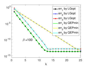
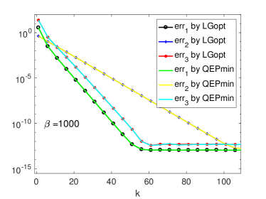
Figure 2: Example 5.1: history of $\operatorname{err}_{1}$, $\operatorname{err}_{2}$ and $\operatorname{err}_{3}$ for the cases where $\beta=100$ (left) and $\beta=1000$ (right).

The convergence histories for $\operatorname{err}_{1}$, $\operatorname{err}_{2}$ and $\operatorname{err}_{3}$ are plotted in Figure 2. It can be seen that all converge to the machine precision. Also $\operatorname{err}_{1}$, $\operatorname{err}_{2}$ and $\operatorname{err}_{3}$ are the same, respectively, at every iteration whether CRQopt (1.1) is solved via QEPmin (2.18) or LGopt (2.13), which is consistent with our theory that solving rLGopt (3.5) is equivalent to solving rQEPmin (3.22).

Example 5.2.

We illustrate the sharpness of the error bounds (4.18) in Theorem 4.2 and the relationship between the convergence rate of our Lanczos algorithm and $\kappa$.

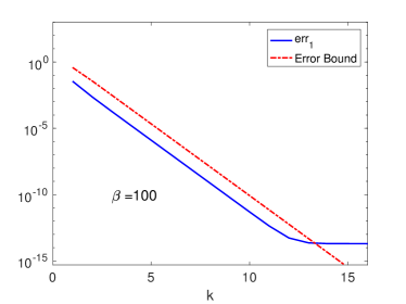
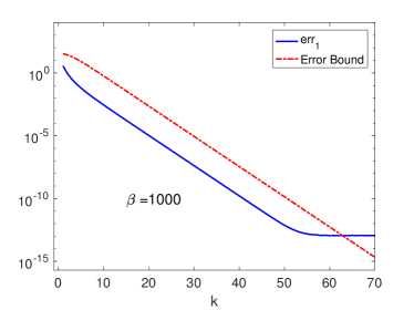
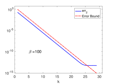
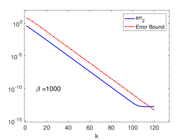
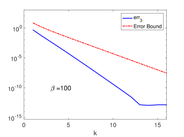
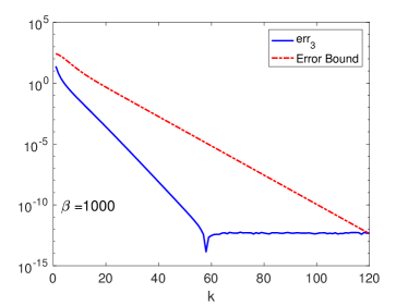
Figure 3: Example 5.2: histories for $\operatorname{err}_{1}$ (first row), $\operatorname{err}_{2}$ (second row), $\operatorname{err}_{3}$ (third row) and their upper bounds for $\beta=100$ (left column) and $\beta=1000$ (right column).

The same test matrices as in Example 5.1, with $\beta=100$ and $1000$ are used. We solve CRQopt (1.1) by solving QEPmin (2.18) and choose the same parameters as in Example 5.1. For $\alpha=1$ and $\beta=100$, We calculate

$$(\lambda_{\ast},\kappa)=\begin{cases}(-42.6007,3.2706),&\quad\mbox{for $(\alpha,\beta)=(1,100)$};\\ (-18.2629,52.8613),&\quad\mbox{for $(\alpha,\beta)=(1,1000)$}.\end{cases}$$

Judging from the corresponding $\kappa$, we expect our Lanczos algorithm will converge faster for the case $\beta=100$ than the case $\beta=1000$. We plot in Figure 3 the convergence histories for

$$\operatorname{err}_{1}\,\, \mbox{and its upper bound $\frac{16\gamma^{2}\|H-\lambda_{\ast}I\|}{v_{\ast}^{\operatorname{T}}Av_{\ast}}\,\left[\Gamma_{\kappa}^{k}+\Gamma_{\kappa}^{-k}\right]^{-2}$ by \eqref{eq:rLGopt-UBs-1}},$$

$$\operatorname{err}_{2}\,\, \mbox{and its upper bound $4\gamma\sqrt{\kappa}\left[\Gamma_{\kappa}^{k}+\Gamma_{\kappa}^{-k}\right]^{-1}$ by \eqref{eq:rLGopt-UBs-2}},$$

$$\operatorname{err}_{3}\,\, \mbox{and its upper bound $\frac{16}{|\lambda_{\ast}|}\|H-\lambda_{\ast}I\|\,\left[\Gamma_{\kappa}^{k}+\Gamma_{\kappa}^{-k}\right]^{-2}+\frac{4}{\gamma|\lambda_{\ast}|}\sqrt{\kappa}\left[\Gamma_{\kappa}^{k}+\Gamma_{\kappa}^{-k}\right]^{-1}$ by \eqref{eq:rLGopt-UBs-3}}.$$

The bounds for $\operatorname{err}_{1}$ and $\operatorname{err}_{2}$ by (4.18a) and (4.18b) for both $\beta=100$ and $\beta=1000$ appear sharp. However, the bound for $\operatorname{err}_{3}$ by (4.18c) is pessimistic. In the plots, $\operatorname{err}_{3}$ goes to $0$ at about a similar rate of $\operatorname{err}_{1}$, but the bounds by (4.18b) and (4.18c) for $\operatorname{err}_{3}$ progress at the same rate as the bound by (4.18a) for $\operatorname{err}_{2}$. We unsuccessfully tried to establish a better bound for $\operatorname{err}_{3}$ to reflect what we just witnessed, but we offered a plausible explanation in Remark 4.3.

As expected, $\operatorname{err}_{1}$, $\operatorname{err}_{2}$ and $\operatorname{err}_{3}$ go to $0$ faster for the case $\beta=100$ than the case $\beta=1000$. It is consistent with our convergence results in Theorem 4.2 that our Lanczos algorithm for CRQopt (1.1) converges faster when $\kappa$ is smaller.

Example 5.3.

We consider an example where the error bounds in Theorem 4.2 are pessimistic, while those by (4.29) can correctly reveal the speed of convergence. This occurs when CRQopt is a “nearly hard case”, i.e., where the optimal value of the corresponding pLGopt (2.24) $\lambda_{\ast}\approx\lambda_{\min}(H)$. Specifically, we choose $n=1100$, $m=100$, $\zeta=0.9$, $a$ a random vector with the norm $1/\zeta$, and

$$H=\operatorname{diag}(\tau_{0\,n-m-2}^{\operatorname{trans}},\tau_{1\,n-m-2}^{\operatorname{trans}},\dots,\tau_{n-m-2\,n-m-2}^{\operatorname{trans}},1)$$

with $(\alpha,\beta)=(2,1000)$ in (5.2) and (5.3), and

$$g_{0}=\left[e^{\eta},e^{2\eta},\cdots,e^{(n-m)\eta}\right]^{\operatorname{T}}$$

where $\eta=-5\times 10^{-3}$. In this case, $\lambda_{\min}(H)=1$ and $\lambda_{\ast}=0.9845$, so $\lambda_{\min}(H)\approx\lambda_{\ast}$ and thus it is a nearly hard case. It is computed that

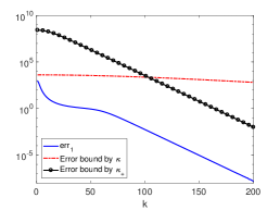
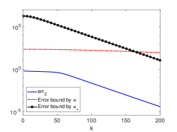
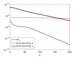
Figure 4: Example 5.3: histories of $\operatorname{err}_{1}$, $\operatorname{err}_{2}$, $err_{3}$ and their upper bounds. “Error bound by $\kappa$” and “Error bound by $\kappa_{+}$” means upper bounds in (4.18) and (4.29), respectively.

$$\kappa=\frac{\lambda_{\max}(H)-\lambda_{\ast}}{\lambda_{\min}(H)-\lambda_{\ast}}\approx 6.4466\times 10^{4}$$

which is big. We solve the associated CRQopt (1.1) via QEPmin (2.18). In Figure 4, we plot the convergence history:

$$\operatorname{err}_{1} \frac{16\gamma^{2}\|H-\lambda_{\ast}I\|}{v_{\ast}^{\operatorname{T}}Av_{\ast}}\,\left[\Gamma_{\kappa}^{k}+\Gamma_{\kappa}^{-k}\right]^{-2}$$ , its upper bounds by (4.18a), and

$$\mbox{$\frac{16\gamma^{2}\|H-\lambda_{\ast}I\|(\theta_{\max}-\theta_{\min})}{(\theta_{\min}-\lambda_{\ast}){v_{\ast}^{\operatorname{T}}Av_{\ast}}}\,\left[\Gamma_{\kappa_{+}}^{(k-1)}+\Gamma_{\kappa_{+}}^{-(k-1)}\right]^{-2}$ by \eqref{eq:bound211}},$$

$$\operatorname{err}_{2} 4\gamma\sqrt{\kappa}\left[\Gamma_{\kappa}^{k}+\Gamma_{\kappa}^{-k}\right]^{-1}$$ , its upper bounds by (4.18b), and

$$\mbox{$4\gamma\sqrt{\kappa}\frac{\theta_{\max}-\theta_{\min}}{\theta_{\min}-\lambda_{\ast}}\left[\Gamma_{\kappa_{+}}^{(k-1)}+\Gamma_{\kappa_{+}}^{-(k-1)}\right]^{-1}$ by \eqref{eq:bound212}},$$

$$\operatorname{err}_{3} \frac{16}{|\lambda_{\ast}|}\|H-\lambda_{\ast}I\|\,\left[\Gamma_{\kappa}^{k}+\Gamma_{\kappa}^{-k}\right]^{-2}+\frac{4\|b_{0}\|}{\gamma|\lambda_{\ast}|}\sqrt{\kappa}\left[\Gamma_{\kappa}^{k}+\Gamma_{\kappa}^{-k}\right]^{-1}$$ , its upper bounds by (4.18c), and

$$\frac{\theta_{\max}-\theta_{\min}}{|\lambda_{\ast}|(\theta_{\min}-\lambda_{\ast})}\left[16\|H-\lambda_{\ast}I\|\,\left[\Gamma_{\kappa_{+}}^{(k-1)}+\Gamma_{\kappa_{+}}^{-(k-1)}\right]^{-2}+\frac{4}{\gamma}\|b_{0}\|\sqrt{\kappa}\left[\Gamma_{\kappa_{+}}^{(k-1)}+\Gamma_{\kappa_{+}}^{-(k-1)}\right]^{-1}\right]$$

$$\mbox{ by \eqref{eq:bound213}}.$$

It can be observed that The error bounds by Theorem 4.2 decay much slower than $\operatorname{err}_{1}$, $\operatorname{err}_{2}$ and $\operatorname{err}_{3}$ in this “near hard case”. This is an example for which $\kappa$ is large but $\kappa_{+}$ is small:

$$\kappa_{+}:=\frac{\theta_{\max}-\lambda_{\ast}}{\theta_{2}-\lambda_{\ast}}\approx 983.7702,$$

As commented in Remark 4.2, sharper bounds like ones by (4.29) should be used. They are also included in Figure 4. We can see that the bounds (4.29) correctly reflect the speed of convergence, but they are bigger than the corresponding errors by several order of magnitudes.

Example 5.4.

In this example, we test the effectiveness of the residual bound $\delta_{k}^{\operatorname{QEPmin}}$ in (3.27). We use the same test problem as in Example 5.1 for both $\beta=100$ and $\beta=1000$. We run our Lanczos algorithm for QEPmin (2.18) and record the residual $\operatorname{NRes}_{k}^{\operatorname{QEPmin}}$ and its bound $\delta_{k}^{\operatorname{QEPmin}}$ defined in (3.27) for every Lanczos step. They are plotted in Figure 5. We observe that both $\operatorname{NRes}_{k}^{\operatorname{QEPmin}}$ and $\delta_{k}^{\operatorname{QEPmin}}$ in (3.27) converge to $0$ at the same rate, suggesting $\delta_{k}^{\operatorname{QEPmin}}$ is an very effective upper bound of the residual $\operatorname{NRes}_{k}^{\operatorname{QEPmin}}$.

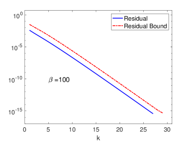
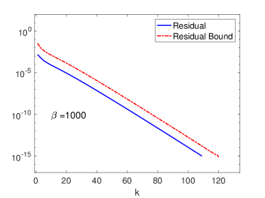
Figure 5: Example 5.4: relative residual of QEP $\operatorname{NRes}_{k}^{\operatorname{QEPmin}}$ and the bound of the relative residual $\delta_{k}^{\operatorname{QEPmin}}$ for the case where $\beta=100$ (left) and $\beta=1000$ (right).

6 Application to the constrained clustering

In this section, we use semi-supervised learning for clustering as an application of CRQopt (1.1). We first discuss unconstrained clustering in Section 6.1 and then discuss a new model for constrained clustering in Section 6.2. Numerical experiments are shown in Sections 6.3 and 6.3.

6.1 Unconstrained clustering

Clustering is an important technique for data analysis and is widely used in machine learning [8, Chapter 14.5.3], bioinformatics [32], social science [26] and image analysis [36]. Clustering uses some similarity metric to group data into different categories. In this section, we discuss the normalized cut, a spectral clustering method that are popular for image segmentation [36, 39].

Given an undirected graph $G=({\cal V},{\cal E})$ whose edge weights are represented by an affinity matrix $W=[w_{ij}]$, we define the cut of a partition on its vertices ${\cal V}$ into two disjoint sets ${\cal A}$ and ${\cal B}$, i.e., ${\cal A}\cup{\cal B}={\cal V}$, ${\cal A}\cap{\cal B}=\emptyset$ as

$$\operatorname{cut}({\cal A},{\cal B})=\sum_{i\in{\cal A},j\in{\cal B}}w_{ij}.$$ (6.1)

Intuitively one would minimize the $\operatorname{cut}$ to achieve an optimal bipartition of the graph $G$, but it often results in a partition $({\cal A},{\cal B})$ with one of them containing only a few isolated vortices in the graph while the other containing the rest. Such a bipartition is not balanced and not useful in practice. To avoid such an unnatural bias that leads to small sets of isolated vortices, the following normalized cut [36] is introduced:

$$\operatorname{Ncut}({\cal A},{\cal B})=\frac{\operatorname{cut}({\cal A},{\cal B})}{\operatorname{vol}({\cal A})}+\frac{\operatorname{cut}({\cal A},{\cal B})}{\operatorname{vol}({\cal B})},$$ (6.2)

where

$$\operatorname{vol}({\cal A})=\sum_{i\in{\cal A},j\in{\cal V}}w_{ij}\quad\mbox{and}\quad\operatorname{vol}({\cal B})=\sum_{i\in{\cal B},j\in{\cal V}}w_{ij}.$$

It turns out that minimizing $\operatorname{Ncut}({\cal A},{\cal B})$ usually yields a more balanced bipartition. Let

$$c_{+}=\sqrt{\frac{\operatorname{vol}({\cal B})}{\operatorname{vol}({\cal A})\cdot\operatorname{vol}({\cal V})}}\quad\mbox{and}\quad c_{-}=-\sqrt{\frac{\operatorname{vol}({\cal A})}{\operatorname{vol}({\cal B})\cdot\operatorname{vol}({\cal V})}},$$

and $x\in\mathbb{R}^{n}$ ($n=|{\cal V}|$, the cardinality of ${\cal V}$) be the indicator vector for bipartition $({\cal A},{\cal B})$, i.e.,

$$x_{(i)}=\left\{\begin{aligned} c_{+},\quad i\in{\cal A},\\ c_{-},\quad i\in{\cal B},\end{aligned}\right.$$ (6.3)

and $D$ be a diagonal matrix with the row sums of $W$ on the diagonal, i.e., $D=\operatorname{diag}(W\mathbf{1})$. Then it can be verified that

$$\operatorname{Ncut}({\cal A},{\cal B})=x^{\operatorname{T}}(D-W)x,\quad x^{\operatorname{T}}Dx=1,\quad(Dx)^{\operatorname{T}}{\bf 1}=0,$$

where ${\bf 1}$ is a vector of ones. Therefore in order to minimize $\operatorname{Ncut}({\cal A},{\cal B})$, we will solve the following combinatorial optimization problem

$$\min~{} x^{\operatorname{T}}(D-W)x,$$ (6.4a)

s.t. $$x_{(i)}\in\{c_{+},\,c_{-}\},$$ (6.4b)

$$x^{\operatorname{T}}Dx=1,$$ (6.4c)

$$(Dx)^{\operatorname{T}}{\bf 1}=0.$$ (6.4d)

However, the problem (6.4) is a discrete optimization problem and known to be NP-complete. A common practice to make it numerical feasible is to relax $x$ to a real vector and solve instead the following optimization problem

$$\min~{} x^{\operatorname{T}}(D-W)x,$$ (6.5a)

s.t. $$x^{\operatorname{T}}Dx=1,$$ (6.5b)

$$(Dx)^{\operatorname{T}}{\bf 1}=0,$$ (6.5c)

$$x\in\mathbb{R}^{n}.$$ (6.5d)

Under the assumption that $D$ is positive definite, by the Courant-Fisher variational principle [13, Sec 8.1.1], solving (6.5) is equivalent to finding the eigenvector $x$ corresponding to the second smallest eigenvalue of the generalized symmetric definite eigenproblem

$$(D-W)x=\lambda Dx.$$

Note that the setting here is different from the one in [36], where the indicator vector $x_{(i)}\in\{1,-b\}$ and $b=\frac{\operatorname{vol}({\cal A})}{\operatorname{vol}({\cal B})}$. Instead of minimizing a quotient of two quadratic functions in [36], we use the constraint that $x^{\operatorname{T}}Dx=1$. The model (6.4) is similar to the one in [39, section 5.1], where they use the number of vertices in the sets ${\cal A}$ and ${\cal B}$ instead of the volumes. The model (6.4) is derived in a similar way to the derivation in [39, section 5.1].

6.2 Constrained clustering

When partial grouping information is known in advance, we can use partial grouping information to set up different models for better clustering. These models are known as constrained clustering. Existing methods for constrained spectral clustering includes implicitly incorporating the constraints into Laplacians [3, 18] and imposing the constraints in linear forms [6, 41, 42] or bilinear forms [40].

We encode the partial grouping information into a linear constraint, which can be either homogeneous [42] or nonhomogeneous [6, 41]. In [6], the authors set up a model where the objective function is the quotient of two quadratic functions and used hard coding for the known associations of pixels to specific classes in terms of linear constraints. In [41], the authors used a model for which the objective function is quadratic and encoded known labels by linear constraints. This is an approach that we take to set up the model.

Let $\mathcal{I}=\{i_{1},\cdots,i_{\ell}\}$ be the index set for which we have the prior information such as ${\cal I}\subseteq{\cal A}$. According to (6.3), we set $x_{(i)}=c_{+}$ for $i\in\mathcal{I}$. Similarly, let $\mathcal{J}=\{j_{1},\cdots,j_{k}\}$ be the index set for which we have the prior information that ${\cal J}\subseteq{\cal B}$, and we set $x_{(j)}=c_{-}$ for $j\in\mathcal{J}$. This leads to the following discrete constrained normalized cut problem

$$\min~{} x^{\operatorname{T}}(D-W)x,$$ (6.6a)

s.t. $$x_{(i)}\in\left\{c_{+},\,c_{-}\right\},$$ (6.6b)

$$x^{\operatorname{T}}Dx=1,$$ (6.6c)

$$(Dx)^{\operatorname{T}}{\bf 1}=0,$$ (6.6d)

$$x_{(i)}=c_{+}\quad\mbox{for}\quad i\in\mathcal{I},$$ (6.6e)

$$x_{(i)}=c_{-}\quad\mbox{for}\quad i\in\mathcal{J}.$$ (6.6f)

However, there are two imminent issues associated with the model (6.6):

1. the combinatorial optimization (6.6) is NP-hard;

2. the model is incomplete because to calculate $c_{+}$ and $c_{-}$ we need to know $\operatorname{vol}({\cal A})$ and $\operatorname{vol}({\cal B})$, which are unknown before the clustering.

Common workarounds, which we use, are as follows. For the first issue, we relax the model (6.6) by allowing $x$ to be a real vector, i.e., $x\in\mathbb{R}^{n}$. For the second issue, we use ${\frac{\operatorname{vol}(\mathcal{J})}{\operatorname{vol}(\mathcal{I})}}$ as an estimate of ${\frac{\operatorname{vol}({\cal B})}{\operatorname{vol}({\cal A})}}$ to get

$$c_{+}\approx\widehat{c}_{+}=\sqrt{\frac{\operatorname{vol}(\mathcal{J})}{\operatorname{vol}(\mathcal{I})\cdot\operatorname{vol}({\cal V})}},\,\,c_{-}\approx\widehat{c}_{-}=-\sqrt{\frac{\operatorname{vol}(\mathcal{I})}{\operatorname{vol}(\mathcal{J})\cdot\operatorname{vol}({\cal V})}}.$$

By these relaxation, we reach a computational feasible model:

$$\min~{} x^{\operatorname{T}}(D-W)x,$$ (6.7a)

s.t. $$x^{\operatorname{T}}Dx=1,$$ (6.7b)

$$(Dx)^{\operatorname{T}}{\bf 1}=0,$$ (6.7c)

$$x_{(i)}=\widehat{c}_{+},\quad i\in\mathcal{I},$$ (6.7d)

$$x_{(i)}=\widehat{c}_{-}.\quad i\in\mathcal{J},$$ (6.7e)

The last three equations are linear constraints and can be collectively written as a linear system of equations:

$$N^{\operatorname{T}}x=b.$$

Let $v=D^{1/2}x$, and define

$$A=D^{-1/2}(D-W)D^{-1/2}\quad\mbox{and}\quad C=D^{1/2}N.$$

Then the optimization problem (6.7) is turned into CRQopt (1.1) with matrices $A$, $C$ and $b$ just defined.

6.3 Numerical results

Experimental setting.

For a grayscale image, we can construct a weighted graph $G=({\cal V},{\cal E})$ by taking each pixel as a node and connecting each pair $(i,j)$ of pixel $i$ and $j$ by an edge with a weight given by

$$w_{ij}=e^{-\frac{\|F(i)-F(j)\|_{2}^{2}}{\delta_{F}}}\times\begin{cases}1&\quad\mbox{if }\|X(i)-X(j)\|_{\infty}<r,\\ 0&\quad\mbox{otherwise},\end{cases}$$ (6.8)

where $\delta_{F}$ and $r$ are chosen parameters, $F$ is the brightness value and $X$ is the location of a pixel [36]. In our experiment, we take

$$\delta_{F}=\delta\max_{i,j}\|F(i)-F(j)\|_{2}^{2}$$

for some parameter $\delta$ to be specified.

The definition of weight in (6.8) ensures that every pixel is connected with an edge to at most $(2r+1)^{2}$ other pixels. As shown in Table 1, in our experiments, $r$ is taken either $5$ or $10$, and thus the weight matrix $W$ is sparse, which in turn makes the matrix $A$ in CRQopt (1.1) sparse, too. Note that for the example Crab, the contrast between the upper right of the object and the background is not significant. Therefore, we choose $r$ to be twice as much as other examples to ensure the weight matrix correctly reflect the connectivity of the graph. In addition, in our experiments $\delta$ is around $0.1$, to be consistent with the statement in [36] that “$\delta_{F}$ is typically set to 10 to 20 percent of the total range of the feature distance function”. Besides, size $m$ of linear constraints is relatively small compared with the number of pixels $n$, yielding CRQopt (1.1) with $m\ll n$.

Table 1: The number of pixels $n$, parameters $\delta$ and $r$ and size $m$ of linear constraints.

Image Number of pixels $n$ $\delta$ $r$ $m$ Flower 30,000 0.1 5 24 Road 50,268 0.1 5 46 Crab 143,000 0.1 10 32 Camel 240,057 0.08 5 24 Dog 395,520 0.1 5 33 Face1 562,500 0.1 5 31 Face2 922,560 0.1 5 19 Daisy 1,024,000 0.08 5 29 Daisy2 1,024,000 0.08 5 59

All experiments were conducted on a PC with Intel Core i7-4770K CPU@3.5GHz and 16-GB RAM. CRQopt (1.1) is solved via solving QEPmin (2.18). In our tests, we choose the maximum Lanczos steps ${\tt maxit}=300$ and use $\delta_{k}^{\operatorname{QEPmin}}<8\times 10^{-5}$ as the stopping criterion. Besides, we choose the minimum Lanczos steps ${\tt minit}=120$ and check the stopping conditions every $5$ Lanczos steps to reduce the cost of checking the stopping conditions.

Quality of the model.

We apply the model (6.7) and Lanczos algorithm for CRQopt (1.1) on different kinds of images and show the results for segmentation and the computed eigenvector in Figure 6. We can see that the image cut results of the model (6.7) indeed agree with our natural visual separation of the object and the background. Daisy and Daisy2 are the same image but with two different ways of prior partial labeling. For both ways of prior partial labelling, the computed image cuts look equally well. Table 2 displays the wall-clock runtime and the numbers of Lanczos steps used for the images.

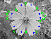
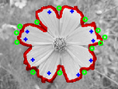
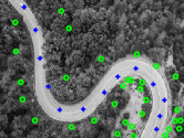
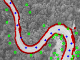
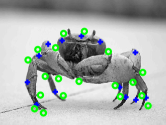
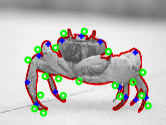
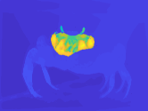
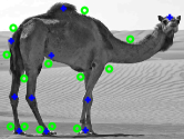
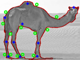
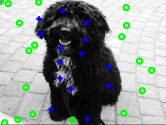
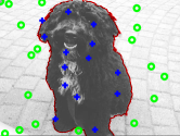
Figure 6: The left, middle and right columns are labels, results of image cut and the heat maps of the solutions by the Lanczos algorithm for CRQopt, respectively. Images from top to bottom are Flower, Road, Crab, Camel, Dog, Face1, Face2, Daisy and Daisy2, respectively.

Table 2: Runtime (in seconds) and number of Lanczos steps

Image Run Time Lanczos steps Flower 4.61 210 Road 14.92 200 Crab 21.58 135 Camel 31.12 300 Dog 22.33 135 Face1 67.46 215 Face2 35.54 165 Daisy 84.09 235 Daisy2 105.80 245

The purpose of experiments on Daisy and Daisy2 which are the same images but with two different ways of labeling is to observe how the size $m$ of the linear constraints may affect running time. Daisy has $29$ linear constraints while Daisy2 has $59$. As shown in Table 2, the Lanczos algorithm took $84.09$ seconds for Daisy and $105.80$ seconds for Daisy2, suggesting the larger $m$ is, the more times the Lanczos algorithm needs, as expected, to solve the associated CQRopt. This is because matrix-vector product $Px$ does more work as $m$ increases.

In Table 3, we show the running time for Fast-GE-2.0 [18], projected power method [41], and the Lanczos algorithm for a few examples. For comparable segmentation quality, the runtime of the Lanczos algorithm for CRQopt (1.1) is significantly less than the existing methods, including Fast-GE-2.0 and the projected power method. For example, with the same prior labeling on the image Crab, Fast-GE-2.0 and the projected power method take $47.13$ seconds and $446.76$ seconds, respectively, while our Lanczos algorithm only takes $21.18$ seconds. Again, with the same labeling on Daisy and Daisy2, Fast-GE-2.0 takes $1572.81$ and seconds $1319.58$ seconds, respectively, the projected power method fails to converge in three hours, while the Lanczos algorithm only takes $84.09$ seconds and $105.80$ seconds, respectively.

Table 3: Runtime for Fast-GE-2.0, projected power method and the Lanczos algorithm

Image Fast-GE-2.0 Projected Power Method Lanczos algorithm Crab 47.13 s 446.76 s 21.58 s Daisy 1572.81 s 3+ hours 84.09 s Daisy2 1319.58 s 3+ hours 105.80 s

7 Conclusions

Although the constrained Rayleigh quotient optimization problem (CRQopt) (1.1), also known as the linear constrained eigenvalue problem, has been around since 1970s, some of the mathematical claims were not rigorously justified. There are not many numerical methods that are suitable for large scale CRQopt (1.1), such as those arising from constrained image segmentation. The projected power method [41] converges too slow while the method in [14] is for the homogeneous constraints only. Eigenvalue optimization method [6] could be too expensive. In this paper, we launched a systematical and rigorous theoretical study of the problem and, as a result, devised an efficient Lanczos algorithm for large scale CRQopt (1.1). We perform a detailed convergence analysis. As an application, we apply our Lanczos algorithm to the image cut problem with partial prior labeling. Numerical experiments on several images demonstrate the effectiveness of the algorithm in terms of accuracy and superior efficiency compared to Fast-GE-2.0 [18] and the projected power method [41]. For future work, our goal is to solve rLGopt (3.5) for nearly hard case and applications of our algorithms on more machine learning problems such as outlier removal [25], semi-supervised kernel PCA [31], and transductive learning [19].

Although our developments in this article have been restricted to the real numbers, their extensions to the complex version of CRQopt (1.1)

$$\min_{v\in\mathbb{C}^{n}}v^{\operatorname{H}}Av\quad\mbox{s.t.}\,\,v^{\operatorname{H}}v=1\,\,\mbox{and}\,\,C^{\operatorname{H}}v=b$$

is rather straightforward, where $A\in\mathbb{C}^{n\times n}$ is Hermitian, i.e., $A=A^{\operatorname{H}}$, $C\in\mathbb{C}^{n\times m}$. Essentially, all we need to do is to replace all transposes ${\,\cdot\,}^{\operatorname{T}}$ by complex conjugate transposes ${\,\cdot\,}^{\operatorname{H}}$.

Appendix A Solve secular equation

We are interested in computing the smallest zero $\lambda_{\ast}$ of the secular function

$$\chi(\lambda):=\sum_{i=1}^{n}\frac{\xi_{i}^{2}}{(\lambda-\theta_{i})^{2}}-\gamma^{2},$$ (A.1)

where it is assumed

$$\gamma>0,\,\,\theta_{1}\leq\theta_{2}\leq\cdots\leq\theta_{n},\,\,\mbox{and},$$

$$\mbox{either $\xi_{1}\neq 0$, or $\xi_{1}=0$ but}\,\,\lim_{\lambda\to\theta_{1}^{-}}\chi(\lambda)>0.$$

Those assumptions guarantee that $\chi(\lambda)$ has a unique zero $\lambda_{\ast}$ in $(-\infty,\theta_{1})$. This is because

$$\lim_{\lambda\to-\infty}\chi(\lambda)=-\gamma^{2}<0,\,\,\lim_{\lambda\to\theta_{1}^{-}}\chi(\lambda)>0,\,\,\mbox{and}\,\,\chi^{\prime}(\lambda)=-2\sum_{i=1}^{n}\frac{\xi_{i}^{2}}{(\lambda-\theta_{i})^{3}}>0\,\,\mbox{for $\lambda<\theta_{1}$}.$$

First, we find an initial lower bound $\alpha^{(0)}$ of $\lambda_{\ast}$, i.e., $\alpha^{(0)}<\theta_{1}$ such that $\chi(\alpha^{(0)})<0$. Note

$$\chi(\lambda)\leq\sum_{i=1}^{n}\frac{\xi_{i}^{2}}{(\lambda-\theta_{1})^{2}}-\gamma^{2}\quad\mbox{for $\lambda<\theta_{1}$}.$$

One such $\alpha^{(0)}$ can be found by solving

$$\sum_{i=1}^{n}\frac{\xi_{i}^{2}}{(\alpha^{(0)}-\theta_{1})^{2}}-\gamma^{2}=0\quad\Rightarrow\quad\alpha^{(0)}=\theta_{1}-\delta_{0}\,\,\mbox{with}\,\,\delta_{0}=\frac{1}{\gamma}\sqrt{\sum_{i=1}^{n}\xi_{i}^{2}}\,.$$

We conclude that $\lambda_{\ast}\in[\alpha^{(0)},\beta^{(0)}]$, where $\beta^{(0)}=\theta_{1}$. Quantities $\alpha^{(k)}$ and $\beta^{(k)}$ will be determined during our iterative process to be described such that $\lambda_{\ast}\in[\alpha^{(k)},\beta^{(k)}]$.

Without loss of generality, we may assume that

if $$\theta_{1}=\cdots=\theta_{d}<\theta_{d+1} \xi_{2}=\cdots=\xi_{d}=0$$, then .

Let

$$j_{0}=\min\{i\,:\,\xi_{i}\neq 0\}.$$ (A.2)

To find the initial guess of the root, we solve

$$\frac{\xi_{j_{0}}^{2}}{(\lambda-\theta_{j_{0}})^{2}}+\underbrace{\sum_{i=j_{0}+1}^{n}\frac{\xi_{i}^{2}}{([\theta_{j_{0}}-\delta_{0}]-\theta_{i})^{2}}-\gamma^{2}}_{=:-\eta}=0$$

for $\lambda$ to get

$$\lambda^{(0)}=\begin{cases}\theta_{j_{0}}-|\xi_{j_{0}}|/\sqrt{\eta},&\quad\mbox{if $\eta>0$},\\ \theta_{j_{0}}-\delta_{0}/2,&\quad\mbox{if $\eta\leq 0$},\end{cases}$$

where the second case is based on bisection.

For the iterative scheme, suppose we have an approximation $\lambda^{(k)}\approx\lambda_{\ast}$. First, the interval $(\alpha^{(k)},\beta^{(k)})$ will be updated as

$$\alpha^{(k+1)}\leftarrow\lambda^{(k)} \beta^{(k+1)}\leftarrow\beta^{(k)} \chi(\lambda^{(k)})<0$$ and if

$$\beta^{(k+1)}\leftarrow\lambda^{(k)} \alpha^{(k+1)}\leftarrow\alpha^{(k)} \chi(\lambda^{(k)})>0$$ and if .

Then we find the next approximation $\lambda^{(k+1)}$. For that purpose, we seek to approximate $\chi$, in the neighborhood of $\lambda^{(k)}$, by

$$g(\lambda):=-b+\frac{a}{(\lambda-\theta_{j_{0}})^{2}}\approx\chi(\lambda),$$

such that

$$g(\lambda^{(k)}) \equiv-b+\hphantom{2}\frac{a}{(\lambda^{(k)}-\theta_{j_{0}})^{2}} =\chi(\lambda^{(k)})=\hphantom{-2}\sum_{i=1}^{n}\frac{\xi_{i}^{2}}{(\lambda^{(k)}-\theta_{i})^{2}}-\gamma^{2},$$

$$g^{\prime}(\lambda^{(k)}) \equiv\hphantom{-b}-2\frac{a}{(\lambda^{(k)}-\theta_{j_{0}})^{3}} =\chi^{\prime}(\lambda^{(k)})=-2\sum_{i=1}^{n}\frac{\xi_{i}^{2}}{(\lambda^{(k)}-\theta_{i})^{3}},$$

yielding

$$a =-\frac{1}{2}(\lambda^{(k)}-\theta_{j_{0}})^{3}\chi^{\prime}(\lambda^{(k)})=(\lambda^{(k)}-\theta_{j_{0}})^{3}\sum_{i=1}^{n}\frac{\xi_{i}^{2}}{(\lambda^{(k)}-\theta_{i})^{3}}>0,$$

$$b =\frac{a}{(\lambda^{(k)}-\theta_{j_{0}})^{2}}-\chi(\lambda^{(k)})=(\lambda^{(k)}-\theta_{j_{0}})\sum_{i=1}^{n}\frac{\xi_{i}^{2}}{(\lambda^{(k)}-\theta_{i})^{3}}-\chi(\lambda^{(k)}).$$

Ideally, $b>0$ so that $g(\lambda)=0$ has a solution in $(-\infty,\theta_{j_{0}})$. Assuming $b>0$, we find the next approximation $\lambda^{(k+1)}\approx\lambda_{\ast}$ is given by

$$\lambda^{(k+1)}=\theta_{1}-\sqrt{a/b}.$$ (A.3)

Now if $b\leq 0$ (then $\lambda^{(k+1)}$ as in (A.3) is undefined) or if $\lambda^{(k+1)}\not\in(\alpha,\beta)$, we let $\lambda^{(k+1)}$ be $(\alpha^{(k+1)}+\beta^{(k+1)})/2$ according to bisection method.

Appendix B Proof of the equivalence between CRQopt and the eigenvalue optimization problem

Suppose $U\in\mathbb{R}^{n\times(n-m)}$ has full column rank and that ${\cal R}(U)={\cal N}(C^{\operatorname{T}})$ and let $u\in\mathbb{R}^{n}$ satisfies $C^{\operatorname{T}}u=\sqrt{n}\,b$. Define

$$\widehat{C}=[C^{\operatorname{T}},\ -\sqrt{n}b],\,\,N=\hbox{}\vbox{\kern 0.86108pt\hbox{$\kern 0.0pt\kern 2.5pt\kern-5.0pt\left[\kern 0.0pt\kern-2.5pt\kern-5.55557pt\vbox{\kern-0.86108pt\vbox{\vbox{ \halign{\kern\arraycolsep\hfil\@arstrut$\kbcolstyle#$\hfil\kern\arraycolsep& \kern\arraycolsep\hfil$\@kbrowstyle#$\ifkbalignright\relax\else\hfil\fi\kern\arraycolsep&& \kern\arraycolsep\hfil$\@kbrowstyle#$\ifkbalignright\relax\else\hfil\fi\kern\arraycolsep\cr 5.0pt\hfil\@arstrut$\scriptstyle$\hfil\kern 5.0pt&5.0pt\hfil$\scriptstyle\scriptscriptstyle n-m$\hfil\kern 5.0pt&5.0pt\hfil$\scriptstyle\scriptscriptstyle 1\\\scriptscriptstyle n$\hfil\kern 5.0pt&5.0pt\hfil$\scriptstyle U$\hfil\kern 5.0pt&5.0pt\hfil$\scriptstyle u\\\scriptscriptstyle 1$\hfil\kern 5.0pt&5.0pt\hfil$\scriptstyle 0$\hfil\kern 5.0pt&5.0pt\hfil$\scriptstyle 1$\hfil\kern 5.0pt\crcr}}}}\right]$}}.$$ (B.1)

and

$$L=N^{\operatorname{T}}\begin{bmatrix}A&0\\ 0&0\end{bmatrix}N,\,\,E=N^{\operatorname{T}}\begin{bmatrix}-\frac{I}{n+1}&0\\ 0&1-\frac{1}{n+1}\end{bmatrix}N,\,\,M=N^{\operatorname{T}}\begin{bmatrix}I_{n}&0\\ 0&0\end{bmatrix}N.$$

Note that it is easy to see that ${\cal R}(N)=\mathcal{N}(\widehat{C})$.

In this appendix we prove that CRQopt (1.1) is equivalent to the following eigenvalue optimization problem

$$\max_{t\in\mathbb{R}}\lambda_{\min}(L+tE,M),$$ (B.2)

where $\lambda_{\min}(L+tE,M)$ is the smallest eigenvalue of $(L+tE)x=\lambda Mx$. This equivalency was initiately established by Eriksson, Olsson and Kahl [6]. However, the statements presented here are stronger than the related ones in [6]. For examples, we will prove $M$ is positive definite, and we can use ’$\max$’ in (B.2) instead of ’$\sup$’ in [6].

Let $\widetilde{v}=\sqrt{n}v$, $\widehat{v}=\begin{bmatrix}\widetilde{v}\\ 1\end{bmatrix}$, $\widehat{A}=\begin{bmatrix}A&0\\ 0&0\end{bmatrix}$, $\widehat{B}=\begin{bmatrix}I_{n}&0\\ 0&0\end{bmatrix}$. Then $v$ is a minimizer of CRQopt (1.1) if and only if $\widehat{v}$ is a minimizer of

$$\min\frac{\widehat{v}^{\operatorname{T}}\widehat{A}\widehat{v}}{\widehat{v}^{\operatorname{T}}\widehat{B}\widehat{v}},\quad\mbox{s.t.}\,\,\widehat{v}_{(n+1)}^{2}=1,\,\,\widehat{v}^{\operatorname{T}}\widehat{v}=n+1,\,\,\widehat{C}\widehat{v}=0.$$ (B.3)

Since ${\cal R}(N)=\mathcal{N}(\widehat{C})$, for any $\widehat{v}$ satisfying $\widehat{C}\widehat{v}=0$, there exists $\widehat{y}\in\mathbb{R}^{n-m+1}$ such that $\widehat{v}=N\widehat{y}$, $N$ is defined in (B.1). By the matrix structure in (B.1), we know that $\widehat{v}_{(n+1)}^{2}=1$ if and only if $\widehat{y}_{(n-m+1)}^{2}=1$. Therefore, solving (B.3) is equivalent to solving

$$\min\frac{\widehat{y}^{\operatorname{T}}L\widehat{y}}{\widehat{y}M\widehat{y}},\quad\mbox{s.t.}\,\,\widehat{y}_{(n-m+1)}^{2}-1=0,\,\,\widehat{y}^{\operatorname{T}}N^{\operatorname{T}}N\widehat{y}=n+1.$$ (B.4)

To prove (B.4) is equivalent to its dual problem, we use the following result on the duality of the quadratic constrained optimization problems.

Lemma B.1 ([6, Corollary 1]).

Let $y^{\operatorname{T}}A_{2}y+2b^{\operatorname{T}}_{2}y+c_{2}$ be a positive semidefinite quadratic form. If there exists $y$ such that $y^{\operatorname{T}}A_{3}y+2b^{\operatorname{T}}_{3}y+c_{3}<0$ and if $A_{3}$ is positive semidefinite, then the primal problem

$$\inf_{y}\frac{y^{\operatorname{T}}A_{1}y+2b_{1}^{\operatorname{T}}y+c_{1}}{y^{\operatorname{T}}A_{2}y+2b_{2}^{\operatorname{T}}y+c_{2}},\quad\mbox{\rm s.t.}\,\,y^{\operatorname{T}}A_{3}y+2b^{\operatorname{T}}_{3}y+c_{3}=0$$

and the dual problem

$$\sup_{\lambda}\inf_{y}\frac{y^{\operatorname{T}}(A_{1}+\lambda A_{3})y+2(b_{1}+\lambda b_{3})^{\operatorname{T}}y+(c_{1}+\lambda c_{3})}{y^{\operatorname{T}}A_{2}y+2b^{\operatorname{T}}_{2}y+c_{2}}$$

has no duality gap.

Proof.

See [6, Corollary 1]. ∎

With the help of Lemma B.1, we have the following theorem to show that that there is no duality gap between the optimization problem (B.4) and its dual problem.

Theorem B.1 ([6, Theorem 1]).

Let $\widehat{A}_{i}=\begin{bmatrix}A_{i}&b_{i}\\ b_{i}^{\operatorname{T}}&c_{i}\end{bmatrix}$ for $i=1,2,3$. If $\widehat{A}_{2}$ and $A_{3}$ are positive semidefinite and if there exists $\widehat{y}$ such that $\widehat{y}^{\operatorname{T}}\widehat{A}_{3}\widehat{y}<n+1$ and $\widehat{y}_{n+1}^{2}=1$, then the primal problem

$$\inf_{y^{\operatorname{T}}A_{3}y+2b^{\operatorname{T}}_{3}y+c_{3}=n+1}\frac{y^{\operatorname{T}}A_{1}y+2b_{1}^{\operatorname{T}}y+c_{1}}{y^{\operatorname{T}}A_{2}y+2b_{2}^{\operatorname{T}}y+c_{2}}=\inf_{\widehat{y}^{\operatorname{T}}\widehat{A}_{3}\widehat{y}=n+1,\widehat{y}_{n+1}^{2}=1}\frac{\widehat{y}^{\operatorname{T}}\widehat{A}_{1}\widehat{y}}{\widehat{y}^{\operatorname{T}}\widehat{A}_{2}\widehat{y}}$$ (B.5)

and its dual

$$\sup_{t}\inf_{\widehat{y}^{\operatorname{T}}\widehat{A}_{3}\widehat{y}=n+1}\frac{\widehat{y}^{\operatorname{T}}\widehat{A}_{1}\widehat{y}-t\widehat{y}_{n+1}^{2}-t}{\widehat{y}^{\operatorname{T}}\widehat{A}_{2}\widehat{y}}$$

has no duality gap.

Proof.

Let $\gamma_{\ast}$ be the optimal value of (B.5), then

$$\gamma_{\ast} =\inf_{\widehat{y}^{\operatorname{T}}\widehat{A}_{3}\widehat{y}=n+1,\widehat{y}_{n+1}^{2}=1}\frac{\widehat{y}^{\operatorname{T}}\widehat{A}_{1}\widehat{y}}{\widehat{y}^{\operatorname{T}}\widehat{A}_{2}\widehat{y}}$$

$$=\sup_{t}\inf_{\widehat{y}^{\operatorname{T}}\widehat{A}_{3}\widehat{y}=n+1,\widehat{y}_{n+1}^{2}=1}\frac{\widehat{y}^{\operatorname{T}}\widehat{A}_{1}\widehat{y}+t\widehat{y}_{n+1}^{2}-t}{\widehat{y}^{\operatorname{T}}\widehat{A}_{2}\widehat{y}}$$

$$\geq\sup_{t}\inf_{\widehat{y}^{\operatorname{T}}\widehat{A}_{3}\widehat{y}=n+1}\frac{\widehat{y}^{\operatorname{T}}\widehat{A}_{1}\widehat{y}+t\widehat{y}_{n+1}^{2}-t}{\widehat{y}^{\operatorname{T}}\widehat{A}_{2}\widehat{y}}$$

$$\geq\sup_{t,\lambda}\inf_{\widehat{y}}\frac{\widehat{y}^{\operatorname{T}}\widehat{A}_{1}\widehat{y}+t\widehat{y}_{n+1}^{2}-t+\lambda(\widehat{y}^{\operatorname{T}}\widehat{A}_{3}\widehat{y}-(n+1))}{\widehat{y}^{\operatorname{T}}\widehat{A}_{2}\widehat{y}}$$

$$=\sup_{t,\lambda}\inf_{\widehat{y}}\frac{{y}^{\operatorname{T}}{A}_{1}{y}+2b_{1}^{\operatorname{T}}y+c_{1}+t\widehat{y}_{n+1}^{2}-t+\lambda({y}^{\operatorname{T}}{A}_{3}{y}+2b_{3}^{\operatorname{T}}y+c_{3}-(n+1))}{{y}^{\operatorname{T}}{A}_{2}{y}+2b_{2}^{\operatorname{T}}y+c_{2}}$$

$$=\sup_{t,\lambda}\inf_{\widehat{y}_{n+1}^{2}=1}\frac{{y}^{\operatorname{T}}{A}_{1}{y}+2b_{1}^{\operatorname{T}}y+c_{1}+\lambda({y}^{\operatorname{T}}{A}_{3}{y}+2b_{3}^{\operatorname{T}}y+c_{3}-(n+1))}{{y}^{\operatorname{T}}{A}_{2}{y}+2b_{2}^{\operatorname{T}}y+c_{2}}$$ (B.6)

$$=\inf_{y^{\operatorname{T}}A_{3}y+2b^{\operatorname{T}}_{3}y+c_{3}=n+1}\frac{y^{\operatorname{T}}A_{1}y+2b_{1}^{\operatorname{T}}y+c_{1}}{y^{\operatorname{T}}A_{2}y+2b_{2}^{\operatorname{T}}y+c_{2}}=\gamma_{\ast},$$ (B.7)

where (B.6) and (B.7) apply Lemma B.1. ∎

Remark B.1.

One of the conditions in [6, Theorem 1] is “$\widehat{A}_{3}$ is positive semidefinite”. However, the proof of Theorem B.1 applies Lemma B.1, which requires $A_{3}$ to be positive semidefinite and there exists $\widehat{y}$ such that $\widehat{y}^{\operatorname{T}}\widehat{A}_{3}\widehat{y}<n+1$ and $\widehat{y}_{n+1}^{2}=1$. Therefore, the condition “$\widehat{A}_{3}$ is positive semidefinite” is not necessary. In addition, in the statement of [6, Theorem 1], one of the constraints is ${y}_{n+1}^{2}=1$. However, in (B.5), the size of the matrix $A_{i}$ and $\widehat{A_{i}}$ is $n\times n$ and $(n+1)\times(n+1)$ for $i=1,2,3$, respectively. Therefore, we consider $y\in\mathbb{R}^{n}$ and $\widehat{y}\in\mathbb{R}^{n+1}$. Therefore, we change the constraint ${y}_{n+1}^{2}=1$ to $\widehat{y}_{n+1}^{2}=1$.

We now prove that the conditions of Theorem B.1 are staisfied for the constrained Rayleigh quotient optimization problem (B.4).

Lemma B.2.

Suppose $\|v_{0}\|<1$, where $v_{0}=(C^{\operatorname{T}})^{\dagger}b$. Then there exists $\widehat{y}$ such that $\|\widehat{y}\|_{N}^{2}=\widehat{y}^{\operatorname{T}}N^{\operatorname{T}}N\widehat{y}<n+1$ and $\widehat{y}_{(n-m+1)}=1$.

Proof.

Note that $v_{0}=(C^{\operatorname{T}})^{\dagger}b$ is the minimum norm solution of $C^{\operatorname{T}}v=b$. Let $\widehat{v}=[\sqrt{n}v_{0}^{\operatorname{T}},1]^{\operatorname{T}}$. Then $\widehat{v}\in\mathcal{N}(\widehat{C})$ and thus there exists $\widehat{y}$ such that $\widehat{v}=N\widehat{y}$ for which we have $\|\widehat{y}\|_{N}=\|\widehat{v}\|_{2}<\sqrt{n+1}$, and, at the same time, $\widehat{y}_{(n-m+1)}=\widehat{v}_{(n+1)}=1$. ∎

By Lemma B.2 and Theorem B.1, the optimization problem (B.4) is equivalent to its dual problem

$$\sup_{t}\inf_{\widehat{y}^{\operatorname{T}}N^{\operatorname{T}}N\widehat{y}=n+1}\frac{\widehat{y}^{\operatorname{T}}L\widehat{y}+t\widehat{y}_{n-m+1}^{2}-t}{\widehat{y}^{\operatorname{T}}M\widehat{y}}.$$ (B.8)

Since

$$t\widehat{y}_{n-m+1}^{2}-t=t\widehat{y}_{n-m+1}^{2}-t\frac{\widehat{y}^{\operatorname{T}}N^{\operatorname{T}}N\widehat{y}}{n+1}=\widehat{y}^{\operatorname{T}}E\widehat{y},$$

(B.8) is equivalent to

$$\sup_{t}\inf_{\widehat{y}^{\operatorname{T}}N^{\operatorname{T}}N\widehat{y}=n+1}\frac{\widehat{y}^{\operatorname{T}}(L+tE)\widehat{y}}{\widehat{y}^{\operatorname{T}}M\widehat{y}}.$$ (B.9)

To transform the dual problem (B.9) to an eigenvalue problem, we first prove that $M$ is positive definite.

Lemma B.3.

Let $b$ be as defined in (1.1c) and $b\neq 0$. $N$ has full column rank, then $M$ is positive definite.

Proof.

It is clear that $M$ is positive semi-definite. We claim that $M$ is nonsingular. Suppose, to the contrary, that $M$ is singular. Then there exists a nonzero $x$ such that $Mx=0$.

We claim that $x_{(n-m+1)}\neq 0$; otherwise suppose $x_{(n-m+1)}=0$ and write $x=\begin{bmatrix}x_{1}\\ 0\end{bmatrix}$. It follows from $Mx=0$ that $U^{\operatorname{T}}Ux=0$, implying $x_{1}=0$ because $U$ has full column rank. Thus $x=0$, a contradiction.

Without loss of generality, we may normalize $x_{(n-m+1)}$ to $1$, i.e., $x=\begin{bmatrix}x_{1}\\ 1\end{bmatrix}$. Note that $M=N^{\operatorname{T}}N-e_{n-m+1}e_{n-m+1}^{\operatorname{T}}$. $Mx=0$ implies $N^{\operatorname{T}}Nx=\begin{bmatrix}0\\ 1\end{bmatrix}$. $N^{\operatorname{T}}N$ is invertible. We now express $(N^{\operatorname{T}}N)^{-1}_{(n-m+1,n-m+1)}$ in two different ways. $N^{\operatorname{T}}Nx=\begin{bmatrix}0\\ 1\end{bmatrix}$ yields $x=(N^{\operatorname{T}}N)^{-1}\begin{bmatrix}0\\ 1\end{bmatrix}$ and thus

$$1=\begin{bmatrix}0\\ 1\end{bmatrix}^{\operatorname{T}}x=\begin{bmatrix}0\\ 1\end{bmatrix}^{\operatorname{T}}(N^{\operatorname{T}}N)^{-1}\begin{bmatrix}0\\ 1\end{bmatrix}=(N^{\operatorname{T}}N)^{-1}_{(n-m+1,n-m+1)}.$$

On the other hand,

$$N^{\operatorname{T}}N=\begin{bmatrix}U^{\operatorname{T}}U&U^{\operatorname{T}}u\\ u^{\operatorname{T}}U&u^{\operatorname{T}}u+1\end{bmatrix}.$$

By the assumption that $U$ has full column rank, $U^{\operatorname{T}}U$ is invertible. With help of a formula of the determinant of block matrices, we have

$$\det(N^{\operatorname{T}}N)=\det(U^{\operatorname{T}}U)\det[(1+u^{\operatorname{T}}u-u^{\operatorname{T}}U(U^{\operatorname{T}}U)^{-1}U^{\operatorname{T}}u].$$

According to the relationship between the inverse and the adjoint of a matrix, we find

$$(N^{\operatorname{T}}N)^{-1}_{(n-m+1,n-m+1)} =(-1)^{n-m+1+n-m+1}\frac{\det(U^{\operatorname{T}}U)}{\det(N^{\operatorname{T}}N)}$$

$$=\frac{\det(U^{\operatorname{T}}U)}{\det(U^{\operatorname{T}}U)\det[(1+u^{\operatorname{T}}u-u^{\operatorname{T}}U(U^{\operatorname{T}}U)^{-1}U^{\operatorname{T}}u]}$$

$$=\frac{\det(U^{\operatorname{T}}U)}{\det(U^{\operatorname{T}}U)[1+u^{\operatorname{T}}(I-P_{U})u]},$$

where $P_{U}$ is the orthogonal projection onto ${\cal R}(U)$. Therefore, $(N^{\operatorname{T}}N)^{-1}_{(n-m+1,n-m+1)}=1$ if and only if $u^{\operatorname{T}}(I-P_{U})u=0$ implying that $u$ is in the column space of $U$. Without loss of generality, we may assume the first column of $U$ is $u$. Now subtract the first column of $N$ from its last column to conclude that $e_{n+1}$ is in the null space of $\widehat{C}$, which contradicts that $b\neq 0$. ∎

By Lemma B.3 and Courant-Fisher minimax theorem [13, Theorem 8.1.2], finding

$$\inf_{\widehat{y}^{\operatorname{T}}N^{\operatorname{T}}N\widehat{y}=n+1}\frac{\widehat{y}^{\operatorname{T}}(L+tE)\widehat{y}}{\widehat{y}^{\operatorname{T}}M\widehat{y}}$$

is equivalent to finding the smallest eigenvalue of $K^{-1}(L+tE)K^{-\operatorname{T}}x=\lambda x$, where $M=KK^{\operatorname{T}}$ is the Cholesky factorization of $M$. Therefore, (B.9) is equivalent to

$$\sup_{t}\lambda_{\min}(L+tE,M).$$ (B.10)

Finally, we prove that the maximum value can be obtained, i.e., ’$\sup$’ in (B.10) can be replaced by ’$\max$’.

Lemma B.4.

Let $f(t)=\lambda_{\min}(L+tE,M)$. There exits $t_{0}\in\mathbb{R}$ such that $f(t_{0})=\sup_{t\in\mathbb{R}}f(t)$.

Proof.

We prove the claim by showing that

$$\lim_{t\rightarrow+\infty}f(t)=\lim_{t\rightarrow-\infty}f(t)=-\infty.$$

First, let $v_{1}\in{\cal R}(N)$ with the last component being zero, and set $y_{1}=N^{\operatorname{T}}v_{1}$. We have $y_{1}^{\operatorname{T}}Ey_{1}=-\frac{\|v_{1}\|^{2}_{2}}{n+1}<0$ and $y_{1}^{\operatorname{T}}My_{1}>0$ since $M$ is positive definite. Hence

$$\lim_{t\rightarrow+\infty}f(t)=\lim_{t\rightarrow+\infty}\inf_{\widehat{y}}\frac{\widehat{y}^{\operatorname{T}}(L+tE)\widehat{y}}{\widehat{y}^{\operatorname{T}}M\widehat{y}}\leq\lim_{t\rightarrow+\infty}\frac{y_{1}^{\operatorname{T}}(L+tE)y_{1}}{y_{1}^{\operatorname{T}}My_{1}}\leq\lim_{t\rightarrow+\infty}t\frac{y_{1}^{\operatorname{T}}Ey_{1}}{y_{1}^{\operatorname{T}}My_{1}}+\lambda_{\max}(L,M)=-\infty.$$

Recall $v_{0}=(C^{\operatorname{T}})^{{\dagger}}b$ and the assumption that $\|v_{0}\|<1$. Let $v_{2}=[\sqrt{n}v_{0}^{\operatorname{T}},\ 1]^{\operatorname{T}}$. Clearly $v_{2}\in{\cal R}(N)$ and let $y_{2}=N^{\operatorname{T}}v_{2}$. We have $y_{2}^{\operatorname{T}}Ey_{2}=-\frac{\|v_{0}\|^{2}_{2}}{n+1}+1-\frac{1}{n+1}>0$ since $\|v_{0}\|<1$ and $y_{2}^{\operatorname{T}}My_{2}>0$ since $M$ is positive definite. Hence

$$\lim_{t\rightarrow-\infty}f(t)=\lim_{t\rightarrow-\infty}\inf_{\widehat{y}}\frac{\widehat{y}^{\operatorname{T}}(L+tE)\widehat{y}}{\widehat{y}^{\operatorname{T}}M\widehat{y}}\leq\lim_{t\rightarrow-\infty}\frac{y_{2}^{\operatorname{T}}(L+tE)y_{2}}{y_{2}^{\operatorname{T}}My_{2}}\leq\lim_{t\rightarrow-\infty}t\frac{y_{2}^{\operatorname{T}}Ey_{2}}{y_{2}^{\operatorname{T}}My_{2}}+\lambda_{\max}(L,M)=-\infty.$$

Therefore, there exits $t_{1}<0$ such that $f(t)<f(0)$ for $t<t_{1}$ and there exits $t_{2}>0$ such that $f(t)<f(0)$ for when $t>t_{2}$. Therefore

$$\sup_{t\in\mathbb{R}}f(t)=\sup_{t\in[t_{1},t_{2}]}f(t).$$

Because $f(t)=\lambda_{\min}(L+tE,M)$ is a continuous function [38], there exists $t_{0}\in[t_{1},t_{2}]$ such that $f(t_{0})=\sup_{t\in\mathbb{R}}f(t)$. ∎

In conclusion, we have shown that CRQopt (1.1) is equivalent to the eigenvalue optimization problem (B.2).

Appendix C CRQPACK

The Lanczos algorithm for solving CRQopt (1.1) described in this paper has been implemented in MATLAB. In the spirit of reproducible research, MATLAB scripts of the implementation of the Lanczos algorithm and the data that used to generate numerical results presented in this paper are packed in a software called package called CRQPACK. CRQPACK can be obtained from

https://www.math.ucdavis.edu/~yszhou/CRQPACK.zip.

CRQPACK consists of three folders:

• src: the source code for solving CRQopt (1.1).

  It consists of four functions CRQ_Lanczos, QEPmin, LGopt and rLGopt. CRQ_Lanczos is the driver and calls QEPmin and LGopt. LGopt is dependent on rLGopt.

  In addition, we also provide two other drivers for solving CRQopt (1.1), namely CRQ_explicit for the direct method [10] and CRQ_ppm for the projected power method [41].

• synthetic: the drivers for numerical examples in section 5.

  correct.m and QEPres.m are for the examples in Sections 5.1 and 5.4, respectively. CRQsharp.m is used to generate the plots for Example 5.2 on error bounds in (4.18a) and (4.18b), while CRQnotsharp.m on the error bounds (4.18a) and (4.18b).

• imagecut: the code for constrained image segmentation.

  It has three subfolders: examples contains the drivers, data contains image data including prior labeling information, and auxiliary contains program to generate the matrices $A$, $C$, and vector $b$ of CRQopt (1.1).

The syntax of calling the driver CRQ_Lanczos is as follows:

[v,info] = CRQopt(A,C,b,opts)

where

• A: the matrix $A$ in CRQopt (1.1)

• C: the matrix $C$ in CRQopt (1.1)

• b: the vector $b$ in CRQopt (1.1)

• opts: option parameters:

  • opts.maxit: maximum number of Lanczos iteraions

  • opts.minit: minimum number of Lanczos iteraions

  • opts.tol: tolerance of relative residual

  • opts.method: method to solve the optimization problem

    1: solve CRQopt via LGopt (default)

    2: solve CRQopt via QEPmin

  • opts.checkstep: the number of Lanczos steps between solving two rLGopt or two rQEPmin and checking the residuals

  • opts.resopt: option for computing the residual (only valid when opts.method=2)

    0 : using residual bound (3.27b) to estimate residual (default)

    1: using residual (3.27a)

  • opts.returnQ: indicator that whether the algorithm returns $Q_{k}$ in structure info

• v: computed solution of CRQopt (1.1)

• info: information for some internal data:

  • info.n0: vector $n_{0}$

  • info.b0: vector $b_{0}$

  • info.gamma2: the square of parameter $\gamma$

  • info.k: the number of Lanczos steps

  • info.T: tridiagonal matrix $T_{k}$

  • info.mu: computed eigenvalue or Lagrange multipliers in each iteration

  • info.res: norms of relative residual of Lagrange equations/QEP in each iteration

  • info.Q: the matrix $Q_{k}$. This field is valid only when opts.returnQ=1

  • info.x: a cell, whose elements are the solutions of all rLGopt (3.5) solved. This field is valid only whenopts.method=1.

  • info.s: a cell, whose element are the eigenvectors of all LEP (3.23) corresponding to the desired eigenvalue. This field is valid only when opts.method=2.

References

- [1] Åke Björck. Numerical Methods for Least Squares Problems. SIAM, Philadelphia, 1996.
- [2] J. R. Bunch, Ch. P. Nielsen, and D. C. Sorensen. Rank-one modification of the symmetric eigenproblem. Numer. Math., 31:31–48, 1978.
- [3] S. E. Chew and N. D. Cahill. Semi-supervised normalized cuts for image segmentation. In Proceedings of the IEEE International Conference on Computer Vision, pages 1716–1723, 2015.
- [4] J. Demmel. Applied Numerical Linear Algebra. SIAM, Philadelphia, PA, 1997.
- [5] N. R. Draper. “Ridge analysis” of response surfaces. Technometrics, 5(4):469–479, 1963.
- [6] A. Eriksson, C. Olsson, and F. Kahl. Normalized cuts revisited: A reformulation for segmentation with linear grouping constraints. Journal of Mathematical Imaging and Vision, 39(1):45–61, 2011.
- [7] D. Fong and M. Saunders. LSMR: An iterative algorithm for sparse least-squares problems. SIAM J. Sci. Comput., 33(5):2950–2971, 2011.
- [8] Jerome Friedman, Trevor Hastie, and Robert Tibshirani. The Elements Of Statistical Learning. Springer, 2001.
- [9] W. Gander. Least squares with a quadratic constraint. Numer. Math., 36:291–307, 1981.
- [10] W. Gander, G. H. Golub, and U. von Matt. A constrained eigenvalue problem. Linear Algebra Appl., 114-115:815–839, 1989.
- [11] I. Gohberg, P. Lancaster, and L. Rodman. Matrix Polynomials. Academic Press, New York, 1982.
- [12] G. H. Golub, M. Heath, and G. Wahba. Generalized cross-validation as a method for choosing a good ridge parameter. Technometrics, 21(2):215–223, 1979.
- [13] G. H. Golub and C. F. Van Loan. Matrix Computations. Johns Hopkins University Press, Baltimore, Maryland, 4th edition, 2013.
- [14] Gene H. Golub, Zhenyue Zhang, and Hongyuan Zha. Large sparse symmetric eigenvalue problems with homogeneous linear constraints: the Lanczos process with inner-outer iterations. Linear Algebra Appl., 309(1):289–306, 2000.
- [15] G. Golubr. Some modified matrix eigenvalue problems. SIAM Rev., 15:318–334, 1973.
- [16] N. I. M. Gould, S. Lucidi, M. Roma, and P. L. Toint. Solving the trust-region subproblem using the Lanczos method. SIAM J. Optim., 9(2):504–525, 1999.
- [17] W. W. Hager. Minimizing a quadratic over a sphere. SIAM J. Optim., 12(1):188–208, 2001.
- [18] C. Jiang, H. Xie, and Z. Bai. Robust and efficient computation of eigenvectors in a generalized spectral method for constrained clustering. In Artificial Intelligence and Statistics, pages 757–766, 2017.
- [19] T. Joachims. Transductive learning via spectral graph partitioning. In Proceedings of the Twentieth International Conference on International Conference on Machine Learning, ICML’03, pages 290–297, 2003.
- [20] J. Lampe and H. Voss. On a quadratic eigenproblem occurring in regularized total least squares. Computational Statistics & Data Analysis, 52(2):1090–1102, 2007.
- [21] R.-C. Li. Solving secular equations stably and efficiently. Technical Report UCB//CSD-94-851, Computer Science Division, Department of EECS, University of California at Berkeley, 1993.
- [22] R.-C. Li. Vandermonde matrices with Chebyshev nodes. Linear Algebra Appl., 428:1803–1832, 2007.
- [23] R.-C. Li. On Meinardus’ examples for the conjugate gradient method. Math. Comp., 77(261):335–352, 2008.
- [24] R.-C. Li. Sharpness in rates of convergence for symmetric Lanczos method. Math. Comp., 79(269):419–435, 2010.
- [25] W. Liu, G. Hua, and J. R. Smith. Unsupervised one-class learning for automatic outlier removal. In 2014 IEEE Conference on Computer Vision and Pattern Recognition, pages 3826–3833, June 2014.
- [26] N. Mishra, R. Schreiber, I. Stanton, and R. E. Tarjan. Clustering social networks. In International Workshop on Algorithms and Models for the Web-Graph, pages 56–67, 2007.
- [27] J. Moré and D. Sorensen. Computing a trust region step. SIAM J. Sci. Statist. Comput., 4(3):553–572, 1983.
- [28] M. E. J. Newman. Spectral methods for community detection and graph partitioning. Phys. Rev. E, 88:042822, 2013.
- [29] C. C. Paige and M. A. Saunders. LSQR: An algorithm for sparse linear equations and sparse least squares. ACM Trans. Math. Software, 8(1):43–71, 1982.
- [30] B. N. Parlett. The Symmetric Eigenvalue Problem. SIAM, Philadelphia, 1998.
- [31] D. Paurat, D. Oglic, and T. Gärtner. Supervised PCA for interactive data analysis. In Proceedings of the Conference on Neural Information Processing Systems (NIPS) 2nd Workshop on Spectral Learning, 2013.
- [32] W. Pentney and M. Meila. Spectral clustering of biological sequence data. In Association for the Advancement of Artificial Intelligence, pages 845–850, 2005.
- [33] F. Rendl and H. Wolkowicz. A semidefinite framework for trust region subproblems with applications to large scale minimization. Math. Program., Ser. A, 77(1):273–299, 1997.
- [34] Y. Saad. Numerical Methods for Large Eigenvalue Problems. Manchester University Press, Manchester, UK, 1992.
- [35] M. A. Saunders. Solution of sparse rectangular systems using LSQR and CRAIG. BIT Numer. Math., 35(4):588–604, 1995.
- [36] J. Shi and J. Malik. Normalized cuts and image segmentation. IEEE Transactions on Pattern Analysis and Machine Intelligence, 22(8):888–905, 2000.
- [37] D. M. Sima, S. Van Huffel, and G. H. Golub. Regularized total least squares based on quadratic eigenvalue problem solvers. BIT Numerical Mathematics, 44(4):793–812, 2004.
- [38] G. W. Stewart and J.-G. Sun. Matrix Perturbation Theory. Academic Press, Boston, 1990.
- [39] U. Von Luxburg. A tutorial on spectral clustering. Statistics and computing, 17(4):395–416, 2007.
- [40] X. Wang, B. Qian, and I. Davidson. On constrained spectral clustering and its applications. Data Mining and Knowledge Discovery, 28(1):1–30, 2014.
- [41] L. Xu, W. Li, and D. Schuurmans. Fast normalized cut with linear constraints. In 2009 IEEE Conference on Computer Vision and Pattern Recognition, pages 2866–2873, June 2009.
- [42] S. X. Yu and J. Shi. Segmentation given partial grouping constraints. IEEE Transactions on Pattern Analysis and Machine Intelligence, 26(2):173–183, 2004.
- [43] L.-H. Zhang, C. Shen, and R.-C. Li. On the generalized Lanczos trust-region method. SIAM J. Optim., 27(3):2110–2142, 2017.