Small, Highly Accurate Quantum Processor for Intermediate-Depth Quantum Simulations

Abstract

Analog quantum simulation is widely considered a step on the path to fault tolerant quantum computation. With current noisy hardware, the accuracy of an analog simulator will degrade after just a few time steps, especially when simulating complex systems likely to exhibit quantum chaos. Here we describe a quantum simulator based on the combined electron-nuclear spins of individual Cs atoms, and its use to run high fidelity simulations of three different model Hamiltonians for ${>}100$ time steps. While not scalable to exponentially large Hilbert spaces, it provides the accuracy and programmability required to explore the interplay between dynamics, imperfections, and accuracy in quantum simulation.

Absent errors, machines that process information according to quantum mechanics can in principle solve problems beyond the computational power of any classical computer. In practice, a scalable, general purpose quantum computer must include error correction and fault tolerance as an integral part of its operation, leading to requirements on the underlying quantum hardware that could be out of reach for years to come Campbell2017 . Thus, in the current era of noisy, intermediate-scale quantum (NISQ) devices Preskill2018 , much of the effort in the field has focused on seemingly less ambitious challenges. High on the list is the development of analog quantum simulators, defined here as devices that operate without error correction but still have the potential to surpass classical computers for tasks such as modeling complex quantum systems Georgescu2014 ; Tacchino2019 . Recent examples include work using traped ions Zhang2017 ; Hempel2018 ; SafaviNaini2018 , Rydberg atoms Labuhn2016 ; Bernien2017 , and superconducting qubits Barends2016 ; Harris2018 to simulate phase transitions and other phenomena in large (${>}50$) spin systems. This is roughly the scale at which numerical modeling on classical computers is currently infeasible.

Quantum simulation generally requires access to highly entangled states of interacting many body systems. It has long been known that such systems also tend to support quantum chaos, in the sense that their time evolution is hypersensitive to perturbation Peres1991 ; Georgeot2000 ; Georgeot2007 . This suggests two separate notions of complexity relevant for quantum simulation, one related to the nature of the quantum state, and another related to the nature of the system dynamics. Entangled states are complex because the information required to predict interparticle correlations grows exponentially with system size, while chaotic dynamics are complex because the information required to predict the quantum trajectory grows exponentially with time Schack1997 . Both will contribute to the overall complexity and fragility of analog quantum simulation and related NISQ-era objectives such as quantum annealing Albash2019 ; Pearson2019 . Indeed, one can expect an inverse relationship between the accessible Hilbert space and the length of time one can meaningfully simulate, with those properties playing a role analogous to the width and depth in quantifying the complexity of a quantum circuit. So far, experiments have focused mostly on the width of a simulation (after all, this is the crucial resource when looking for a quantum advantage), with limited attention paid to the fidelity of the output state as one seeks to increase its depth in terms of simulated time. Yet, to fully understand the computational power of an analog quantum simulation, it is necessary to look carefully at the accessible simulation depth and how it depends on the nature of the dynamics, before one can trust its outcome Hauke2012 .

In this letter we present a new platform for analog quantum simulation (AQS) with tradeoffs that are complementary to NISQ devices: it is modest in terms of accessible Hilbert space, but highly accurate and therefore uniquely suited to the study of dynamical complexity in time. Our small, highly accurate quantum (SHAQ) simulator is based on the combined electron-nuclear spins of individual Cs atoms in the electronic ground state, driven by phase modulated radio-frequency (rf) and microwave ($\mu$w) magnetic fields, and provides access to a fixed $16$-dimensional Hilbert space formally equivalent to four qubits. In place of the quantum circuit model where control is predicated on access to a universal gate set, we rely on a universal control Hamiltonian and quantum Optimal Control Merkel2008 ; Smith2013 to ensure that our simulator is fully programmable, in the sense that we can implement arbitrary unitary maps with average fidelities ${>}0.98$ Anderson2015 . We show that Optimal Control can be further adapted for AQS, allowing us to set up coarse-grained simulations of the dynamics driven by arbitrary model Hamiltonians. Thus, while Optimal Control does not scale to exponentially large Hilbert spaces, it delivers a combination of flexibility and accuracy that is uniquely suited for AQS on SHAQ hardware. We demonstrate experimental AQS of three different spin Hamiltonians on the same device, for ${>}100$ time steps with average fidelity ${>}0.99$ per step. Our work stands out by directly measuring the fidelity of the evolving quantum state as a simulation proceeds. This is the ultimate metric for accuracy, yet quantum state fidelity is rarely reported in contemporary AQS experiments with NISQ hardware, perhaps because indirect measures based on quantum state tomography involve complex protocols that are prone to their own errors SosaMartinez2017 . For examples of other ways to estimate fidelity without resorting to full quantum state tomography, see Flammia2011 ; daSilva2011 ; Lanyon2017 ; Elben2020 . More conventionally, we demonstrate experimental AQS of the time evolution of a bulk observable (magnetization), with a simulation depth and accuracy that lies well beyond the capabilities of universal simulators based on current NISQ hardware (see, for example, refs. Lanyon2011 ; Chiesa2019 ; Smith2019 ; Gustafson2019 ). These are key elements required for future exploration of the interplay between dynamics, hardware imperfections, and accuracy in AQS.

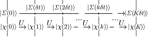
Figure 1: Analog Quantum Simulation. Top: The system evolves continuously from the initial state $|{\it\Sigma}(0)\rangle$ to the final state $|{\it\Sigma}(K\delta t)\rangle$ according to the system Hamiltonian. Bottom: The simulator evolves from the initial state $|\chi(0)\rangle$ to the final state $|\chi(K)\rangle$, coinciding with the system state at intervals $k{=}0,1,2,...,K$.

AQS falls into two broad categories sometimes referred to as “emulation” and “simulation”. A quantum emulator is a special-purpose device governed by the same Hamiltonian and having the same Hilbert space structure as the system of interest. Emulators have been realized on a variety of physical platforms and used to study a range of phenomena with considerable success Zhang2017 ; Britton2012 ; Jurcevic2014 ; Gross2017 . A quantum simulator, by contrast, is a universal device that is controllable, in the sense that one can “program” it to implement any $\text{SU}(d)$ map of Hilbert space onto itself. Given an arbitrary system Hamiltonian and a mapping of the system Hilbert space $\mathscr{H}_{\text{sys}}$ onto the simulator Hilbert space $\mathscr{H}_{\text{sim}}$, one can then implement unitary time steps on the simulator and iterate to perform stroboscopic simulations of the system dynamics (Fig. 1).

Our Cs-atom based “device” is a quantum simulator in the second sense, and requires unitary control over the entire accessible Hilbert space. As shown in Merkel2008 , the spin degrees of freedom of a Cs atom in its electronic ground state are controllable with a combination of phase modulated rf and $\mu$w magnetic fields whose piecewise constant phases $\{\phi_{i}^{\text{rf}x}{,}\phi_{i}^{\text{rf}y}{,}\phi_{i}^{\mu\text{w}}\}{=}\{\vec{\phi}_{i}\}$, $1{\leq}i{\leq}N_{\phi}$, serve as control variables (“controls” for short). We can then apply the generic toolbox of quantum Optimal Control to find (non-unique) controls that accomplish the control task at hand. In this article we focus on the adaptation of Optimal Control to AQS, and refer the reader to past work Merkel2008 ; Smith2013 ; Anderson2015 ; SosaMartinez2017 and SupplementalMaterial for details of the laboratory implementation.

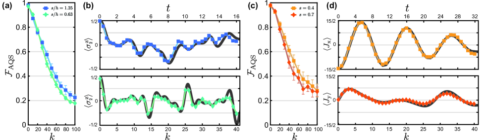
Figure 2: (Color online) AQS of two popular model systems corresponding to the Hamiltonians in Eqs. 2a,b. (a) Measured $\mathcal{F}_{\mathrm{AQS}}(k)$ for two versions of the TI model with $\delta t{=}0.4,s/h{=}1.25$ (squares) and $\delta t{=}0.4,s/h{=}0.63$ (diamonds). (b) Simulation results for $\langle\sigma_{2}^{z}\rangle$ at $\delta t{=}0.4,s/h{=}1.25$ (top) and $\delta t{=}0.4,s/h{=}0.63$ (bottom). (c) Measured $\mathcal{F}_{\mathrm{AQS}}(k)$ for two versions of the LMG model with $\delta t{=}0.8,s{=}0.4$ (squares) and $\delta t{=}1.6,s{=}0.7$ (diamonds). (d) Simulation results for $\langle J_{x}\rangle$ at $\delta t{=}0.8,s{=}0.4$ (top) and $\langle J_{y}\rangle$ at $\delta t{=}0.8,s{=}0.7$ (bottom). Thin lines connect the data points to guide the eye. Thick solid lines in (b) and (d) shows predictions of the exact model. Error bars are the standard error of the mean for the chosen sample of initial states.

To set up an AQS we first choose orthonormal bases in $\mathscr{H}_{\text{sys}}$ and $\mathscr{H}_{\text{sim}}$. Having done so, a straightforward way of mapping from system to simulator is to represent states and operators by identical vectors and matrices in the two bases. Next, given a unitary time propagator $W$ acting on the system, we seek controls $\{\vec{\phi}_{i}\}$ for which the transformation $U(\{\vec{\phi}_{i}\})$ acting on the simulator is a good approximation to $W$. Note that $W$ can be chosen as the exact propagator for a time step of any length; there will be no Trotter errors Georgescu2014 ; Tacchino2019 unless deliberately introduced as part of the simulation. Given $W$, we then use one of two versions of Optimal Control to find high-performing controls:

Conventional Control. This version uses an objective function $\mathcal{F}(\{\vec{\phi}_{i}\}){=}|\text{Tr}[W^{\dagger}U(\{\vec{\phi}_{i}\})]|^{2}/{d^{2}}$ (the fidelity). Numerical optimization of $\mathcal{F}(\{\vec{\phi}_{i}\})$ as a function of $\{\vec{\phi}_{i}\}$ will find controls for which the matrices $W$ and $U(\{\vec{\phi}_{i}\})$ are near identical in the chosen bases. That is, within a global phase, they have the same eigenvalues and eigenstates. In prior work we have found that $N_{\phi}{=}150$ phase steps (450 phase values) is sufficient to consistently achieve a theoretical $\mathcal{F}(\{\vec{\phi}_{i}\}){\geq}0.99999$ for any $W$. In the laboratory where control errors and decoherence are present, the corresponding controls achieve $\mathcal{F}{\geq}0.98$ on average, as measured by randomized benchmarking Anderson2015 .

EigenValue Only (EVO) Control. In AQS there are in principle no restrictions on the map from system to simulator. To take advantage of this, we note that it suffices for $W$ and $U(\{\vec{\phi}_{i}\})$ to have near identical eigenvalues, in which case $W$ and $VU(\{\vec{\phi}_{i}\})V^{\dagger}$ will be nearly identical for some $V$. Accordingly, the EVO approach uses an objective function

$$\mathcal{F}_{\mathrm{EVO}}(\{\vec{\phi}_{i}\}{,}\{v_{j}\}){=}\frac{1}{d^{2}}|\text{Tr}[W^{\dagger}VU(\{\vec{\phi}_{i}\})V^{\dagger}]|^{2}$$ (1)

where $V{=}e^{iA}$, $A{=}\sum_{j=1}^{d^{2}-1}v_{j}\Lambda_{j}$, $\{\Lambda_{j}\}$ is a set of generalized Gell-Mann matrices forming a basis of traceless hermitian $d{\times}d$ matrices, and $\{v_{j}\}$ is a set of $d^{2}{-}1$ real-valued variables, sufficient to generate all $V{\in}\text{ SU}(16)$. Simultaneous optimization of $\mathcal{F}_{\mathrm{EVO}}(\{\vec{\phi}_{i}\}{,}\{v_{j}\})$ with respect to $\{\vec{\phi}_{i}\}$ and $\{v_{j}\}$ will then find co-optimal controls and system-simulator maps.

Our experience suggests the search complexity and computational effort is comparable for Conventional and EVO Control. Furthermore, we find that optimizing for EVO rather than the entire $W$ can reduce the number of phase steps from $N_{\phi}{=}150$ to something in the range from $N_{\phi}{=}10$ to $N_{\phi}{=}60$, depending on the nature of $W$. This brings a significant advantage in terms of the possible number of time steps and overall fidelity in an AQS. On the downside we have found that EVO Control performs poorly when $W$ is close to the identity. This is generally not an issue for AQS where one typically chooses time steps that change the state appreciably. A second issue arises if the system Hamiltonian is time dependent and the propagators $W(k)$ are different for different time steps $k$. One must then do separate EVO searches for solutions $V_{k}U_{k}(\{\vec{\phi}_{i}\})V_{k}^{\dagger}$, where inevitably $V_{k}{\neq}V_{k+1}$. The resulting basis mismatch means one cannot simply concatenate the $U_{k}(\{\vec{\phi}_{i}\})$, and any attempt to restrict the $V_{k}$’s negates the original advantage. Therefore, when necessary, we revert to Conventional Control which works in every scenario we have explored. See SupplementalMaterial for details.

To establish the baseline performance of our quantum simulator we have tested it on three popular model systems described by the Hamiltonians

$$H_{\text{TI}}={-}\sum_{i{=}1}^{N}h\sigma_{i}^{z}{-}\sum_{i{=}1}^{N{-}1}s\sigma_{i}^{x}\sigma_{i{+}1}^{x},\quad{N=4}$$ (2a)

$$H_{\text{LMG}}={-}(1{-}s)J_{z}{-}sJ_{x}^{2},\qquad J=15/2$$ (2b)

$$H_{\text{QKT}}={-}pJ_{z}\sum_{n{=}0}^{\infty}\delta(\tau{-}nT){-}\frac{\kappa}{2JT}J_{x}^{2},\quad J=15/2$$ (2c)

The nearest-neighbor Transverse Ising (TI) Suzuki2013 and Lipkin-Meshkov-Glick (LMG) Lipkin1965 ; Zibold2010 models are common paradigms for the study of phase transitions, and while integrable they nevertheless feature nontrivial dynamics. The Quantum Kicked Top (QKT) is a time-discrete version of the LMG model whose classical phase space can be regular, mixed or globally chaotic depending on the parameters $p,\kappa$ Haake1987 ; Chaudhury2009 . For each model we choose the system size $N$ or $J$ to use the entire $16$-dimensional Hilbert space available on our simulator.

In the laboratory each AQS follows the same basic template. Given a model Hamiltonian, we use Conventional or EVO Control to find controls $\{\vec{\phi}_{i}\}$ and a corresponding propagator $U(\{\vec{\phi}_{i}\})$ that simulates the system evolution during a time step $\delta t$. Knowing the system-simulator map, we then prepare the simulator in the chosen initial state $|\chi(0)\rangle$, take $k$ time steps, measure the observable $M$ of interest, and repeat for $1{\leq}k{\leq}K$ to build up a stroboscopic record of the expectation value $\langle M(k)\rangle$. In AQS of systems such as the TI and LMG models, $M$ might be a spin observable. As a measure of the accuracy of the simulation we can also look at the fidelity of the quantum state itself, $\mathcal{F}_{\mathrm{AQS}}(k){=}\text{Tr}[\rho_{\text{a}}(k)|\chi(k)\rangle\langle\chi(k)|]$, where $|\chi(k)\rangle$ and $\rho_{\text{a}}(k)$ are the predicted and actual states after $k$ steps. To access this quantity we measure the projector $M(k){=}|\chi(k)\rangle\langle\chi(k)|$, i. e., the probability of finding the simulator in the predicted state after $k$ steps. In practice, using laser cooling to prepare a large sample of non-interacting Cs atoms allows us to run as many as $10^{7}$ identical quantum simulators in parallel. This leads to small variations in the control fields from atom to atom, but ensures excellent averaging over noise in the controls and the measurement. In our setup the time per phase step is $4\mu$s and the maximum overall duration of a quantum simulation is $12$ms, limited by the time a free-falling atom spends in the region of uniform control fields.

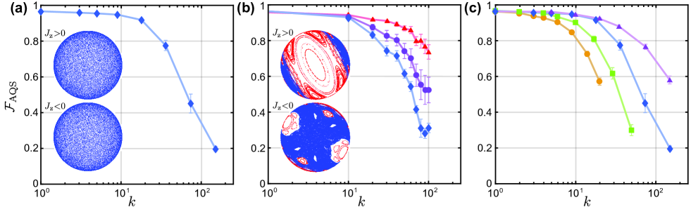
Figure 3: (Color online) AQS of the Quantum Kicked Top, Eq. 2c. (a) Measured $\mathcal{F}_{\mathrm{AQS}}(k)$, averaged over 10 initial coherent states, in the globally chaotic regime $(p{=}1{,}\kappa{=}7)$ . Insert: Classical phase space map for the hemispheres $J_{z}{>}0$ and $J_{z}{<}0$ showing global chaos. (b) Measured $\mathcal{F}_{\mathrm{AQS}}(k)$ in a mixed regime $(p{=}0.99,\kappa{=}2.3)$, averaged over $5$ initial coherent states in the large regular island in the $J_{z}{>}0$ hemisphere (triangles), over $5$ initial coherent states in the sea of chaos in the $J_{z}{<}0$ hemisphere (diamonds), and over all $10$ initial states (circles). Insert: Classical phase space map. (c) Measured $\mathcal{F}_{\mathrm{AQS}}(k)$ ($p{=}1{,}\kappa{=}7)$, averaged over $10$ initial coherent states, for different control strategies: Conventional Control with $N_{\phi}{=}150,K{=}20$ (circles), EVO Control with $N_{\phi}{=}60,K{=}50$ (squares) and $N_{\phi}{=}20,K{=}150$ (diamonds), and finally randomized EVO Control with $N_{\phi}{=}20,K{=}150$ where coherent errors are scrambled (triangles). Thin lines connect the data points to guide the eye. Error bars are the standard error of the mean for the chosen sample of initial states

Figures 2a,c show $\mathcal{F}_{\mathrm{AQS}}(k)$ for two versions of a $4$-site TI model and a $J{=}15/2$ LMG model, each for $0{\leq}k{\leq}100$ time steps. The simulations use EVO Control with $N_{\phi}{=}20$ phase steps, the fidelities are averages over $10$ randomly chosen initial states, and the cut-off at $K{=}100$ is to ensure the fidelity of the time steps does not vary with $k$. The TI data corresponds to ferromagnetic and paramagnetic regimes respectively, while the LMG data correspond to regimes below and just above the critical point. In all cases the simulation fidelity declines smoothly with time but remains well above that of a mixed state, $\mathcal{F}_{\mathrm{AQS}}(k){>}1/16{=}0.0625$, even after $k{=}100$ time steps. As examples of AQS of dynamical observables, Figs. 2b,d show simulations of $\langle\sigma_{2}^{z}\rangle$ for the TI model, and collective spin components $\langle J_{x}\rangle$ and $\langle J_{y}\rangle$ for the LMG model; these examples were chosen because of their varied and nontrivial behavior. Each AQS extends over $1{\leq}k{\leq}40$ time steps, enough to densely sample for long enough that the nature of the dynamics becomes apparent. Overall, quantum simulation of the TI model appears somewhat more challenging than the LMG model, but both track the spin dynamics with good accuracy. Notably, $40$ time steps is enough for a considerable loss of fidelity, $\mathcal{F}_{\mathrm{AQS}}(k){\sim}0.5$, showing that useful simulation of physical observables can be achieved even when accuracy at the level of the quantum state is fairly poor.

As a third test we apply our simulator to the Quantum Kicked Top. An AQS of the QKT consists of repeated applications of the Floquet Operator, and the only meaningful time step is one period of $H_{\mathrm{QKT}}.$ This assures that the propagator $W$ is far from the identity for all but a small subset of parameters, and thus ideally suited for EVO Control. Figs. 3a,b show fidelities $\mathcal{F}_{\mathrm{AQS}}(k)$ for two versions of the QKT with globally chaotic $(p{=}1,\kappa{=}7)$ and mixed $(p{=}0.99,\kappa{=}2.3)$ phase spaces, averaged over $10$ initial coherent states of the collective spin. Based on general arguments relating quantum chaos to hypersensitivity Peres1991 , one might expect that AQS will be more challenging for the globally chaotic case than for the mixed case, and this may explain the lower fidelity seen for the former. For the mixed case we can separate out initial states in regular versus chaotic regions, with the former achieving significantly higher fidelity than the latter. Somewhat counter to expectations, however, every AQS of the QKT shown here does at least as well, and in some case significantly better in terms of fidelity per step, than AQS of the integrable TI and LMG models.

Finally, we use the QKT in the globally chaotic regime to explore how the fidelity of an AQS depends on the control strategy and the errors present in the experiment. Figure 3c shows simulation fidelities for three scenarios: EVO Control with $N_{\phi}{=}20$ and $N_{\phi}{=}60$ phase steps, and Conventional Control with $N_{\phi}{=}150$; the corresponding maximum number of QKT steps are $K{=}150$, $K{=}50$, and $K{=}20$, and the fidelities decline smoothly to $\mathcal{F}_{\mathrm{AQS}}(k){\sim}0.2$, $\mathcal{F}_{\mathrm{AQS}}(k){\sim}0.3$, and $\mathcal{F}_{\mathrm{AQS}}(k){\sim}0.58$ at the end points. To our knowledge, this demonstrates an accessible simulation depth that compares favorably with current state of the art for AQS on NISQ hardware.

It is worth recalling that every AQS discussed here involves repeated application of the time propagator over and over again, a scenario in which coherent control errors have the potential to compound much faster than random noise. We can explore the role of coherent errors versus noise by comparing to a scenario akin to randomized benchmarking Knill2008 . To do so, we use EVO optimization with $N_{\phi}{=}20$ to find a number of time propagators $U(\{\vec{\phi}_{i}\})$, all with identical eigenvalues but different and effectively random controls $\{\vec{\phi}_{i}\}$ and maps $V$. These are put together in random sequences of various lengths, at the end of which we measure the fidelity of the output state relative to the output predicted in the absence of errors. As seen in Figure 3c, the resulting decline in fidelity is significantly slower than for each of the three quantum simulations, with an end point fidelity of $\mathcal{F}_{\mathrm{AQS}}(k){\sim}0.6$ at $k{=}150$, and an average fidelity per step of $0.997$. We take this as evidence that quantum simulations such as those studied here are more strongly affected by coherent errors than random noise, and that efforts to improve the simulation fidelity should focus on the former.

In conclusion, we have demonstrated a small, universal and highly accurate analog quantum simulator based on the spin-degrees of freedom in the ground state of individual Cs atoms. We have further shown how Optimal Control can be adapted to program such a simulator, and we have established its baseline performance by applying it to both integrable and chaotic model systems. Notably, the idea of looking for co-optimal controls and system-simulator maps is not restricted to quantum simulation, and could lead to similar gains in other contexts where a generic control task is mapped onto a specific piece of hardware. Going forward, we plan to use our Cs atom quantum simulator to develop and test a general model of the interplay between the native errors of a generic quantum simulator and the types of observables one might use it to access. Ultimately, we hope testbeds such as ours can help better understand the computational power of analog quantum devices and their use in lieu of error corrected and fault tolerant quantum computers.