Curvature, a mechanical link between the geometrical complexities of a fault.

Abstract

Many recent studies have tried to determine the influence of geometry of faults in earthquake mechanics. In this paper, we suggest a new interpretation of the effect of geometry on the stress on a fault. Starting from the representation theorem, which links the displacement in a medium to the slip distribution on its boundary, and assuming homogeneous infinite medium, a regularized boundary-element equation can be obtained. Using this equation, it is possible to separate the influence of geometry, as expressed by the curvatures and torsions of the field line of a dislocation on the fault surface, which multiply the slip, from the effect of the gradient of slip. This allows us to shed new light on the mechanical effects of geometrical complexities on the fault surface, with the key parameters being the curvatures and torsions of the slip field on the fault surface. We have used this new approach to explain further the false paradox between smooth-and-abrupt-bends (see Sato et al., (2019)) as well as to re-interpret the effect of roughness on a fault.

1 Introduction

The geometry of a fault has an effect on the mechanics of earthquakes, as has been supported by many studies, including observations (King and Nabelek,, 1985; Wesnousky,, 2006, 2008; Bletery et al.,, 2016), theoretical work (Poliakov et al.,, 2002; Rice et al.,, 2005), and numerical modeling (Aochi et al., 000b, ; Bhat et al.,, 2004; Oglesby,, 2005; Li and Liu,, 2016; Ando et al.,, 2017; Romanet et al.,, 2018; Ando and Kaneko,, 2018). Although it is now easy to study the consequences of geometry from numerical models, the underlying mechanics remain unsolved. All faults present some degree of geometrical complexities; it can be a curved subduction zone along the strike, like Sumatra or Cascadia, bends or kinks, or maybe even multiple faults and branches. Even at smaller scales, faults presents complexities. In fact it has been shown that faults are rough on scales covering more than nine orders of magnitude (Candela et al.,, 2012). Knowing that geometrical complexities are present at all scales and that they do have effects, one natural question is whether we can actually discriminate among all the geometrical complexities to see which one has the strongest effect. How exactly does the geometry come into play in the mechanics of an earthquake? In this paper we use elastodynamics to shed new light on these questions from an analytical perspective.

Our starting point is to take advantage of a regularized boundary-element equation, first recalling some established results. We start from the representation theorem, which links the slip on a fault to the resulting displacement everywhere in the medium (Aki and Richards,, 2002):

$$\begin{split}u_{n}(\mathbf{x},t)&=\int_{0}^{t}\iint_{\Sigma}\Delta u_{i}(\mathbf{y},\tau)c_{ijpq}n_{j}(\mathbf{y})\frac{\partial}{\partial y_{q}}G_{np}(\mathbf{x},t-\tau;\mathbf{y},0)\mathrm{d}\Sigma(\mathbf{y})\mathrm{d}\tau.\end{split}$$ (1)

Here $u_{n}(\mathbf{x},t)$ represents the $n$-th component of the displacement, at location $\mathbf{x}$ and time $t$. $c_{ijpq}$ is the Hooke tensor, $n_{j}$ is the $j$-th component of the vector normal to the fault, $\Delta u_{i}(\mathbf{y},\tau)$ is the $i$-th component of the slip on the fault, and $G_{np}(\mathbf{x},t-\tau;\mathbf{y},0)$ is the $n$-th component of the Green’s function, due to a delta function in component $p$ at location $\mathbf{y}$. Finally, $\Sigma$ represents the surface of the fault and $\tau$ the time history of the fault. From this equation, by assuming an elastic medium it is possible to derive the boundary-integral equation that relates the slip on the fault to the stresses everywhere in the medium. By an abuse of language, we will use the word ”slip”, to refer either to the shear slip or the opening in the following of the paper. Using Hooke’s law, and noting that the stress $\sigma_{ab}$is given by:

$$\sigma_{ab}=c_{abcd}\left(\frac{\partial u_{d}}{\partial x_{c}}+\frac{\partial u_{c}}{\partial x_{d}}\right),$$ (2)

we can derive the boundary-integral equations after some algebra (Tada and Yamashita, (1997); Tada et al., (2000)):

$$\sigma_{ab}(\mathbf{x},t)=c_{abcd}\int_{0}^{t}d\tau\iint_{\Sigma}\Delta u_{i}c_{ijpq}n_{j}\frac{\partial}{\partial y_{q}}\frac{\partial}{\partial x_{d}}G_{cp}d\Sigma.$$ (3)

This equation is difficult to interpret because the slip is expressed in a general coordinate system, and also because, this equation is hypersingular (Martin et al.,, 1989) (this integral naturally diverges, but can be evaluated if we use Hadamard finite part definition of the integral). A way to be able to physically interpret this integral is to regularize it.

2 Fundamental results

Following various authors (Sladek and Sladek, (1983),Bonnet, (1999) p345), we introduce the tangential differential operator $D_{ij}=n_{i}\dfrac{\partial}{\partial x_{j}}-n_{j}\dfrac{\partial}{\partial x_{i}}$, where $n_{i}$ represents the i-th componant of the vector $\mathbf{n}$ normal to the surface. Using this operator and assuming a linear, elastic, infinite, homogenous medium allows to perform the regularization of eq. (3) by using integration by parts (Sladek and Sladek, (1984); Bonnet, (1999) p 175). More details are given in appendix A. For the connection with the local coordinate system that has frequently been adopted in the rock mechanics literature (e.g., Tada and Yamashita, (1997); Tada et al., (2000)) please refer to Sato et al., (2019).

$$\begin{split}\sigma_{ab}(\mathbf{x},t)&=c_{abcd}\int_{0}^{t}d\tau\iint_{\Sigma}c_{ijpq}D_{jd}[\Delta u_{i}]G_{cp}d\Sigma\\ &-c_{abcd}\int_{0}^{t}d\tau\iint_{\Sigma}\rho\frac{\partial^{2}}{\partial t^{2}}\Delta u_{i}n_{d}G_{ic}d\Sigma\end{split}$$ (4)

Figure 1: Figure showing the four curvatures of a fault in 3D medium. The curve in red is the field line of tangential slip, as projected onto the fault. The blue line is the field line perpendicular to the field line of tangential slip at every point. The color of the surface represents the elevation.

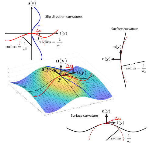
This equation can be interpreted by projecting the derivatives and the slip onto a local coordinate system that is chosen as follows (see Fig. 1): the tangential vector $\mathbf{t}$ is parallel to the projection of the slip vector $\Delta\mathbf{u}$ on the surface at any point, and $\mathbf{s}$ is the perpendicular cotangent vector; the slip vector has no component on $\mathbf{s}$. The last step is to separate the contributions from shear slip and opening: $\Delta u_{i}=t_{i}\Delta u^{t}+n_{i}\Delta u^{n}$. By doing so, it is possible to write the integral in eq. (4) in a form involving different contributions with physical meanings: the effects of the slip gradients (the second and third lines of eq. 5 below), the effects of the curvatures ($\kappa^{t}$, $\kappa^{s}$, $\kappa^{\parallel}$, and $\kappa^{\bot}$ ) and the torsions ($\tau^{t}$ and $\tau^{s}$) of the slip field lines on the fault surface multiplying the slip (the fourth and fifth lines of eq. 5), and the effect of inertia (the sixth line of eq. 5).

$$\begin{split}&\sigma_{ab}(\mathbf{x},t)=\\ &\text{\text@underline{Gradient of slip:}}\\ &c_{abcd}\int_{0}^{t}\iint_{\Sigma}c_{ijpq}\frac{\partial}{\partial x_{q}}G_{cp}(n_{d}t_{j}-n_{j}t_{d})\\ &\qquad\qquad\qquad\qquad\qquad\left[t_{i}\frac{\partial}{\partial y^{t}}\Delta u^{t}+n_{i}\frac{\partial}{\partial y^{t}}\Delta u^{n}\right]d\Sigma d\tau\\ +&c_{abcd}\int_{0}^{t}\iint_{\Sigma}c_{ijpq}\frac{\partial}{\partial x_{q}}G_{cp}(n_{d}s_{j}-n_{j}s_{d})\\ &\qquad\qquad\qquad\qquad\qquad\left[t_{i}\frac{\partial}{\partial y^{s}}\Delta u^{t}+n_{i}\frac{\partial}{\partial y^{s}}\Delta u^{n}\right]d\Sigma d\tau\\ &\text{\text@underline{Curvature and torsion times slip:}}\\ +&c_{abcd}\int_{0}^{t}\iint_{\Sigma}c_{ijpq}\frac{\partial}{\partial x_{q}}G_{cp}(n_{d}t_{j}-n_{j}t_{d})\\ &\qquad\qquad\left[(\kappa^{t}n_{i}+\kappa^{\parallel}s_{i})\Delta u^{t}+(\tau^{t}s_{i}-\kappa^{t}t_{i})\Delta u^{n}\right]d\Sigma d\tau\\ +&c_{abcd}\int_{0}^{t}\iint_{\Sigma}c_{ijpq}\frac{\partial}{\partial x_{q}}G_{cp}(n_{d}s_{j}-n_{j}s_{d})\\ &\qquad\qquad\left[(\tau^{s}n_{i}+\kappa^{\bot}s_{i})\Delta u^{t}-(\kappa^{s}s_{i}+\tau^{s}t_{i})\Delta u^{n}\right]d\Sigma d\tau\\ &\text{\text@underline{Inertia term:}}\\ -&c_{abcd}\int_{0}^{t}\iint_{\Sigma}\frac{\partial^{2}}{\partial t^{2}}\Delta u_{i}(\mathbf{y},\tau)n_{d}\rho G_{ic}d\Sigma d\tau\end{split}$$ (5)

This equation allows us to understand better the different sources of stress due to a slip distribution on a fault. The last term is the inertial term, which is due to the second derivative of slip with time; it disappears when the fault is no longer slipping for a sufficiently long time. The other terms are each constructed in a similar manner:

$$\begin{split}&\int_{0}^{t}\iint_{\Sigma}\underbrace{c_{abcd}c_{ijpq}\frac{\partial}{\partial x_{q}}G_{cp}(n_{d}t_{j}-n_{j}t_{d})}_{\text{Kernel}}\\ &\qquad\qquad\underbrace{\left[(\kappa^{t}n_{i}+\kappa^{\parallel}s_{i})\Delta u^{t}+(\tau^{t}s_{i}-\kappa^{t}t_{i})\Delta u^{n}\right]\vphantom{c_{abcd}c_{ijpq}\frac{\partial}{\partial x_{q}}G_{cp}(n_{d}t_{j}-n_{j}t_{d})}}_{\text{Source}}d\Sigma d\tau.\end{split}$$ (6)

There are two different kernels, which differ only in the projection onto the fault, and two different sources. One novelty of the present work is that the source is not only the gradient of the slip along the fault, called the dislocation, but in addition another kind of source arises from the curvatures and torsion that multiply the slip. This is not the first time that a curvature term has been found in the development of a boundary-element equation. Koller et al., (1992) found a similar term for the dynamic antiplane case in which the boundary-element equation is fully regularized (i.e., there is no Cauchy integral to evaluate). However, our work is truly different from the curvature term as treated in the anti-plane case of Koller et al., (1992), where the traction becomes null when the dislocation goes to zero. The curvature and torsion terms in our work do not vanish when the dislocation is null. These curvatures and torsions are fully defined by the field line of the slip on the fault surface (e.g., the red line in Fig. 1). Interestingly, the kernels for both source contributions are exactly the same. The interpretation of the curvatures and torsions is as follows (see Fig. 1): two are related to the curvature of the fault surface, respectively parallel to the direction of slip projected onto the fault ($\kappa^{t}$), and perpendicular to that projection of the slip direction ($\kappa^{s}$). We call these two terms ”fault-surface curvatures”, because they are related to the geometry of the fault. The other two curvatures are related to changes in the direction of slip projected onto the fault: the change in the direction of the slip itself ($\kappa^{\parallel}$) and the change in the perpendicular direction ($\kappa^{\bot}$); hence, we call them ”slip-direction curvatures” (strictly speaking, we should call them geodetic curvatures). The two last terms are the torsions $\tau^{t}$ and $\tau^{s}$ (strictly speaking, the relative torsions). They can be thought of as the conjugate effect of the geometry of the fault and the change in direction of the slip. The stress due to tangential slip depends only on one fault-surface curvature, the one that is in the direction of the slip. It also depends on the two slip-direction curvatures and one torsion. On the other hand, the stress due to opening does not depend on the slip-direction curvatures, but only on the fault-surface curvatures and torsions. This provides a fundamental difference between the non-planar geometry of opening and shear cracks: although other inertial and gradient contributions can be exactly the same, the contribution from the curvatures and torsions is fundamentally different.

3 Results and discussion

Figure 2: a) Illustration of the smooth-and-abrupt-bend paradox. Calculation of the stresses yields different results for a smooth bend (left panel) or an abrupt bend (right panel), even in the limit of infinitesimally small segments. b) Sketch showing the need for a minimum lengthscale when considering linear elasticity, which is required by the small-strain assumption; the ratio $\Delta u/\lambda_{\text{min}}$ must remain small.

3.1 Relationship to previous work

The work of Tada and Yamashita, (1997); Tada et al., (2000) was done independently of the regularization process using the tangential differential operator. They regularized the boundary-integral equations by projecting the derivative into the local coordinate system and then performing an integration by parts. However, they made a mistake in performing the integration by parts, because they neglected the derivative of the local coordinate system. Their work was corrected by Sato et al., (2019). The apparent smooth-and-abrupt-bend paradox (Tada and Yamashita,, 1996) that results from this omission states that for two bends, one connected with a smooth curve and another connected with straight-line segments (see. Fig. 2.a), the stress calculation yields different results, even in the limit of infinitesimally small straight segments. Through numerical calculation, Sato et al., (2019) showed that this apparent paradox is not correct. This also means that there is no problem in using flat elements to model a curve fault. The work done by Aochi et al., 000a , in which they first calculate the effect of a constant slip rate on a small flat element and then assemble these flat elements (by rotation and translation) to create a complex geometry therefore encounters no problem regarding the smooth-and-abrupt-bend paradox. The use of the tangential differential operator avoid the choice of a local basis along the fault, so this provides an unified view of the derivation, independently of the choice of the coordinate system.

3.2 A geometrical effect

The effects of the curvatures and torsions of the fault surface are truly geometrical effects. This is quite different from the effect of the slip gradient, which can easily be positive or negative on the fault surface and which can evolve with time and eventually reverse sign to fulfill the requirement due to friction applying in the fault. However, if we assume that the geometry of the fault and the direction of the shear slip do not change, the curvature term that multiplies the slip can only evolve monotonically. This means that we expect high stress concentrations at all geometrical complexities, where ”geometrical complexities” stands for any part of the fault where the local curvature is high. In addition to damage, breaks in the free surface, another means for decreasing this stress is actually to decrease the fault-surface curvatures, i.e., to make the fault become flatter. Qualitatively, this effect is observed for mature faults with high slip; they tend to be flatter than the youngest faults.

If one is interested only in the displacement produced by a slip distribution on a fault, there is no such effect of curvature (see eq. (1)). A way to understand this, is to think of the curvature terms multiplied by the slip as a strain (the same way the gradient of slip is also a strain). The geometry still has an influence through the Green’s function, but the curvature is not a source term. Because of this, the assumption of local planarity of a fault for slip inversion is probably a good first approximation. However, as soon as one wants to calculate the strains or stresses, the planar-fault assumption and the true geometrically complex fault gives rise to completely different results: the curvature contribution is neglected, although we have shown that this term can be dominant. This means that one must take care in calculating the stress from slip inversion. Locally on the fault, the true stress state (partly because of the complex local geometry) is probably very different from the one calculated by assuming a locally planar fault. In other words, it is not because two slip distributions are similar that the strain calculated from them is close, because it also depends strongly on the geometry. Another direct consequence is that dynamic (as opposed to kinematic) inversions of the slip on faults are probably very difficult to implement other than statistically, as there is no way to know the exact geometry of a fault.

3.3 In plane elasticity with no opening

The previous result is very general, and it holds for any fault geometry, including multiple faults, in the dynamic case, and it allows for shear slip as well as for opening. To explore this new finding, let us simplify this expression to in-plane elastostatic problem with no opening. In 2D, the torsions and slip direction curvatures disappear, and only one surface curvature remains. In this particular case, the stress in the medium depends only on one curvature mutiplying the shear slip and on the gradient of shear slip along the fault:

$$\begin{split}&\sigma_{ij}(\mathbf{x})=\\ &\int_{C}K_{ij}^{\text{curv}}(\mathbf{x}-\mathbf{y})\kappa^{t}\Delta u^{t}dL(\mathbf{y})+\int_{C}K_{ij}^{\text{grad}}(\mathbf{x}-\mathbf{y})\frac{\partial}{\partial y^{t}}\Delta u^{t}dL(\mathbf{y}).\end{split}$$ (7)

The two kernels $K_{ij}^{\text{curv}}(\mathbf{x}-\mathbf{y})$ and $K_{ij}^{\text{grad}}(\mathbf{x}-\mathbf{y})$ are given in appendix B.1. The difference from the paper of Tada and Yamashita, (1997), is the term involving the curvature in eq. (7), because that reference neglected the derivative of the local coordinate system.

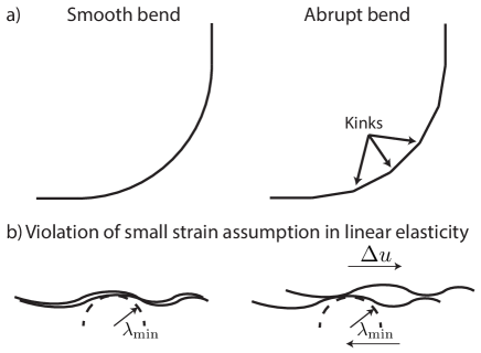
3.3.1 Existence of a lengthscale related to geometry in numerical models (small strain elasticity)

If we want the stress to remain finite in eq. (7), for any geometry, we need to assume a finite curvature along the fault. Otherwise, the slip must vanish at the point of divergent curvature. This also means that, if we want the stress to remain finite at a kink, the only solution is that the slip must be null at the position of the kink. This limitation arises from the fact that these equations were derived in the small-strain approximation (i.e.: linear elasticity): two asperities in contact cannot slide past other each other, as this would break the assumption of small-strains (see Fig. 2.b). In modeling, we are limited by the fact we want to have some slip on the fault, and this necessarily introduces a minimum lengthscale $\lambda_{\text{min}}$ into the system. In practice, the slip has to be much smaller than the curvature: $\Delta u\ll\lambda_{\text{min}}$. Obviously, this is a rather arbitrary limit to the small asperities in modeling, so how can we deal with this lengthscale? One way would be to go beyond the small-strain approximation and use non-linear elasticity. But then the equation become much more complex to solve numerically. Another way would be to incorporate some of the small-scale asperities into the friction law. Such small-lengthscale asperities probably have very localized effects, and therefore this may be sufficient for numerical modeling without using the more complicated tools of non-linear elasticity. Future research is needed to understand the effects of this minimum lengthscale. Another related topic is that one must take care not to break the small-strain assumption of linear elasticity when incorporating roughness in modeling. If we set the minimum roughness to be $\lambda_{\text{min}}=10^{-2}\mathrm{mm}$, and if we assume that linear elasticity holds for maximum strains of $5\%$, this means that the displacement on a fault can be no more than $5\times 10^{-4}\mathrm{mm}$.

3.3.2 Bends and kinks

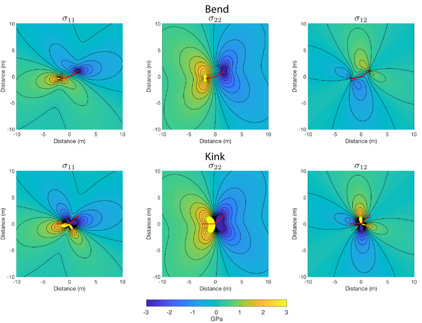
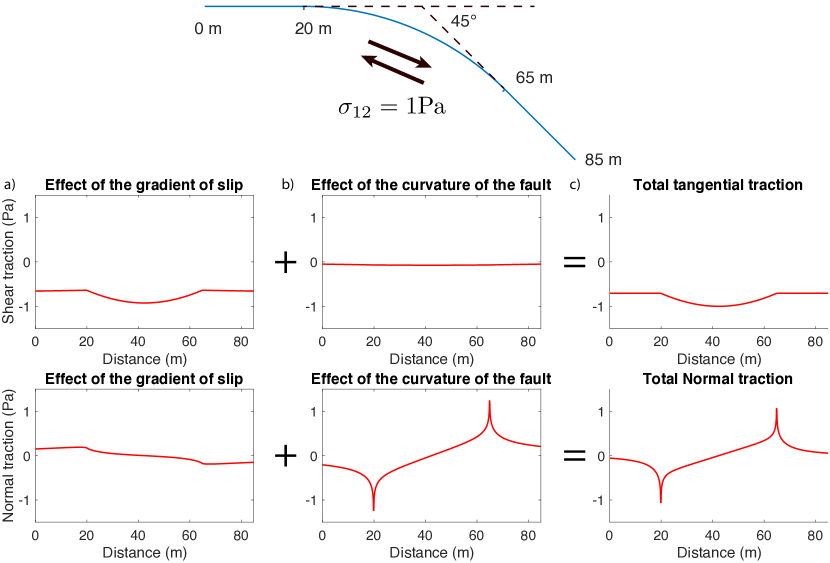
The difference between bends and kinks is an interesting question in the community of fault modeling. Our work allows us to make the link between the two. As stated earlier, the only natural solution when a kink arises on a single fault is for the slip to be zero at the kink. In Fig. 3, we compare the effects of a kink and a smooth bend on the stress. For this purpose, we calculated the effect of a constant tangential slip on a kink and on a bend (the effect of the gradient of slip along the fault is therefore null). This figure shows that the contribution of a kink and a bend on the far field is the same, which provide further evidence to show that the smooth-and-abrupt-bend paradox is wrong (Sato et al.,, 2019). Imagine that we zoom out on the bend, so that we cannot distinguish it anymore; then the solution will be similar to that for a kink. This is rather good news, as it respects the Saint Venant’s principle that ”the difference between the effects of two different but statically equivalent loads becomes very small at sufficiently large distances from load”. If we look at the near field, however, the kink has a singular stress, which the smooth bend does not have. This arises because we imposed a non-zero slip at the kink, which breaks the small-strain assumption of linear elasticity. From the distinction between the effect of the gradient of slip and the effect of the curvature that multiplies the slip, we also can analyze again Figure 2 of Tada and Yamashita, (1996) which shows the normal traction along a bended crack (the total shear stress on the fault, including the elastic and loading shear stress, has to be zero). This figure is similar to Fig. 4, where we distinguish between the traction arising from the gradient of slip and the traction arising from the curvature. The difference between these results arises from the fact that they neglected the curvature term. Note that in this example, the normal traction comes mainly from the curvature term, and the gradient of slip has a smaller influence. Conversely, the effect of curvature on the shear stress is small, and it opposes movement. In this case, the effect of the gradient of slip is preponderant. In summary, a kink can be seen as the limiting case of an infinitesimally small smooth bend. And the terms that matter for understanding the difference between an abrupt bend and a smooth bend is really the curvature term.

Figure 3: Stress in a medium, due to a bend (upper panels), and due to an abrupt bend (lower panels). The slip is constant over the fault. We removed the effect of gradient at the edges of the fault. The angle of aperture is 45°.

Figure 4: The effect of the different contributions of source terms on a curved fault (upper panel), with the assumption that the shear traction is null on the fault. a) Effect of the gradient of slip along the fault on the normal and shear traction. b). Effect of the curvature that multiplies slip along the fault on the normal and shear traction.. c) Total effects on the normal and shear traction on the fault.

3.3.3 Rough faults

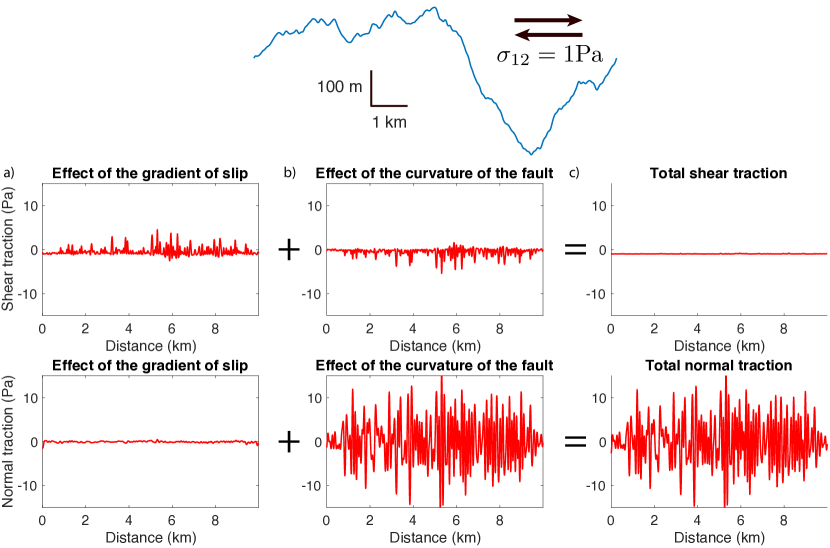
Rough faults have received heightened attention recently because of their effects in earthquake dynamics. It is known that faults actually present roughness at all scales (Power et al., (1987); Power and Tullis, (1991); Renard et al., (2006); Candela et al., (2009, 2012)). Analytical studies of roughness by boundary perturbations always find a scaling of stress that is proportional to slip, the inverse of the minimum lengthscale of roughness, and the shear modulus (Dunham et al., (2011); Fang and Dunham, (2013)). This is in contradiction with the boundary method developed in Tada and Yamashita, (1997); Tada et al., (2000). Our results actually confirms this scaling in a more general way, as we found that it is possible to separate the two contributions. To prevent the equation (7) from diverging, it now appears clearly that a minimum roughness must be set.This also provides an explanation for the difference in roughness measurements in the direction of slip, and perpendicular to the direction of slip (Power et al.,, 1987; Power and Tullis,, 1991; Lee and Bruhn,, 1996). Indeed, we can assume that faults rarely open, so that there is only shear slip on it. The resulting stresses from the shear slip depend only on the curvature in the same direction as the slip ($\kappa^{t}$). The stress increasing with ongoing shear slip, it makes sense that the roughness, by some damage process, will vanish with ongoing slip (Sagy et al., (2007); Brodsky et al., (2011)). Figure 5 shows the contribution of the gradient of slip and the curvature, for a rough crack with an amplitude-to-wavelength ratio $\alpha=10^{-2}$, that is loaded with pure shear. Similar to the bend in Fig. 4, the shear traction depends mainly on the gradient of slip, while the normal traction depends mainly on the curvature that multiplies the slip. The normal stress shows large variations, more than 10 times the initial shear stress drop. The curvature term also seems to correspond to the drag stress found by Fang and Dunham, (2013): the effect of curvature on shear stress opposes the movement of the fault. In this case, the effect of geometry cannot be neglected. As discussed previously, a purely rough fault without a minimum lengthscale $\lambda_{\text{min}}$ can not be modeled using linear elasticity. The curvature would be infinite for such a fault, and therefore the only solution would be that the slip is null.

Figure 5: The effect of the different contributions of source terms on a rough fault (upper panel), with the assumption that the shear traction is null on the fault. a) Effect of the gradient of slip along the fault on the normal and shear traction. b). Effect of the curvature that multiplies slip along the fault on the normal and shear traction.. c) Total effects on the normal and shear traction on the fault.

4 Conclusion

In this paper we have demonstrated the key role of fault curvature in earthquake mechanics. By using regularized boundary-integral equations, we are able to separate the stress contribution into several terms: terms that are proportional to the slip gradient and terms that are proportional both to slip and to the curvatures of the fault. This helps us to understand better the mechanics of fault systems. We have also provided additional arguments which demonstrates that there is no such a thing as a paradox of smooth-and-abrupt-bends (Tada and Yamashita, (1996); Aki and Richards, (2002), p591, Sato et al., (2019)). We have also used this results to generalize recent finding about roughness stress drag and its particular scaling, proportional to slip and the inverse of a minimum lengthscale. We find that the effect of curvature, and therefore geometry is not negligible, even for small departures from a planar fault. The potential applications of this finding are large, and for the first time this work has provided a quantitative way of measuring the effect of geometry of faults on the stresses. This finding can help to understand better, for example, the effect of assuming a planar fault compared to a non-planar fault. This can help to argue that bends and kinks are acting as a barrier, for example, in the case of paleoseismology. This can also help to understand the variation of roughness along the faults, depending on the direction of slip. Finally, we find that the curvature of a fault is the key physical parameter that unifies and defines a complex geometry.

Author contribution statement

P.R. wrote the manuscript. D.S. initially found the regularization technics of the boundary-integral equation. P.R. found the effect of curvature and the implications in 2D. Both D.S. and P.R. participated in combining the two works and discussed the results. R.A. initiated the project and found the mistake in the work of Tada and Yamashita, (1997). Finally, all the three authors have read and approved the present manuscript.

Ackowledgement

P.R would like to acknowledge valuable discussions with Dr. Bhat and Dr. Aochi. P.R. thanks greatly Dr. Ide for allowing him to come to the University of Tokyo. We greatly thank Dr. Bonnet for drawing us attention on the use of the tangential differential operator. P.R also thanks greatly Prof. Madariaga for comments it gets while he was writing this article. The matlab codes used to generate the figures are in supplementary material. This work was partially supported by JSPS KAKENHI 18KK0095 and 19K04031. P.R. received support from KAKENHI 16H02219. D.S was partially supported by JSPS/MEXT KAKENHI Grant Numbers JP26109007.

Appendix A Derivation of regulatised boundary-integral equations

A.1 Green’s function

Here, we recall some properties of the Green’s function of homogeneous linear elastic medium. The Green’s function have some symmetry properties:

$$G_{ij}(\mathbf{x},t,\mathbf{y},\tau)=G_{ij}(\mathbf{x}-\mathbf{y},t-\tau,0,0)$$ (8)

That leads to the following property for the derivative of the Green function:

$$\frac{\partial}{\partial x_{q}}G_{ij}(\mathbf{x},t,\mathbf{y},\tau)=-\frac{\partial}{\partial y_{q}}G_{ij}(\mathbf{x},t,\mathbf{y},\tau)$$ (9)

The Green’s function also satisfied the momemtum balance equation:

$$\begin{split}\rho\frac{\partial^{2}}{\partial t^{2}}G_{in}&=c_{ijpq}\frac{\partial}{\partial x_{j}}\frac{\partial}{\partial x_{q}}G_{pn}\end{split}$$ (10)

A.2 Regularisation of the representation theorem

In this section, we present a regularisation of the representation theorem for general fault geometry following Bonnet, (1999), p174-176. For that purpose, the tangential differential operator $D_{ij}[\sim]$ will be introduced (Sladek and Sladek,, 1983; Bonnet,, 1999):

$$D_{ij}[f]=n_{i}\frac{\partial}{\partial x_{j}}f-n_{j}\frac{\partial}{\partial x_{i}}f$$ (11)

Where $f$ is the function at which the tangential differential operator is applied.

Let us start from the representation theorem:

$$u_{n}(\mathbf{x},t)=\int_{0}^{t}d\tau\iint_{\Sigma}\Delta u_{i}(\mathbf{y},\tau)c_{ijpq}n_{j}\frac{\partial}{\partial y_{q}}G_{np}(\mathbf{x},t-\tau;\mathbf{y},0)d\Sigma$$ (12)

Using the strain stress relationship,

$$\sigma_{ab}=c_{abcd}\frac{1}{2}\left(\frac{\partial u_{d}}{\partial x_{c}}+\frac{\partial u_{c}}{\partial x_{d}}\right)$$ (13)

It is possible to derive the stress:

$$\begin{split}\sigma_{ab}(\mathbf{x},t)&=c_{abcd}\int_{0}^{t}d\tau\iint_{\Sigma}\Delta u_{i}(\mathbf{y},\tau)\\ &\ c_{ijpq}n_{j}\frac{\partial}{\partial y_{q}}\frac{\partial}{\partial x_{d}}G_{cp}(\mathbf{x},t-\tau;\mathbf{y},0)d\Sigma\end{split}$$ (14)

If now we use the property of Green’s function (9), the tangential differential operator and the equation of motion, we can show that:

$$\begin{split}c_{ijpq}n_{j}\frac{\partial}{\partial x_{d}}\frac{\partial}{\partial y_{q}}G_{cp}&=-c_{ijpq}n_{j}\frac{\partial}{\partial x_{d}}\frac{\partial}{\partial x_{q}}G_{cp}\\ &=-c_{ijpq}D_{jd}\frac{\partial}{\partial x_{q}}G_{cp}-c_{ijpq}n_{d}\frac{\partial}{\partial x_{j}}\frac{\partial}{\partial x_{q}}G_{cp}\\ &=-c_{ijpq}D_{jd}\frac{\partial}{\partial x_{q}}G_{cp}-n_{d}\rho\frac{\partial^{2}}{\partial t^{2}}G_{ic}\end{split}$$ (15)

We can rewrite the stress as following:

$$\begin{split}\sigma_{ab}(\mathbf{x},t)&=c_{abcd}\int_{0}^{t}d\tau\iint_{\Sigma}\Delta u_{i}(\mathbf{y},\tau)c_{ijpq}D_{jd}[G_{cp}]d\Sigma\\ &-c_{abcd}\int_{0}^{t}d\tau\iint_{\Sigma}-\Delta u_{i}(\mathbf{y},\tau)n_{d}\rho\frac{\partial^{2}}{\partial t^{2}}G_{ic}d\Sigma\end{split}$$ (16)

After performing integration by parts it comes:

$$\begin{split}\sigma_{ab}(\mathbf{x},t)&=c_{abcd}\int_{0}^{t}d\tau\iint_{\Sigma}c_{ijpq}D_{jd}[\Delta u_{i}(\mathbf{y},\tau)]G_{cp}d\Sigma\\ &-c_{abcd}\int_{0}^{t}d\tau\iint_{\Sigma}\frac{\partial^{2}}{\partial t^{2}}\Delta u_{i}(\mathbf{y},\tau)n_{d}\rho G_{ic}d\Sigma\end{split}$$ (17)

Where we use the fact that:

$$\begin{split}\int_{0}^{t}d\tau\iint_{\Sigma}D_{jd}[c_{abcd}c_{ijpq}\Delta u_{i}(\mathbf{y},\tau)G_{cp}]d\Sigma=0\end{split}$$ (18)

This is derived from Stoke’s theorem (Bonnet, (1999),p346). This regularised boundary-equation (eq. (17)) matches with the expression of Sato et al., (2019), where instead of using the tangential differential operator, the projection of the derivatives on a local basis on the fault is used.

A.3 Derivation of curvature and torsion terms

Using Darboux frame, it can be shown that:

$$\begin{split}\frac{\partial}{\partial y^{t}}\mathbf{t}(\mathbf{y})&=\kappa^{t}\mathbf{n}(\mathbf{y})+\kappa^{\parallel}\mathbf{s}(\mathbf{y})\\ \frac{\partial}{\partial y^{t}}\mathbf{n}(\mathbf{y})&=-\kappa^{t}\mathbf{t}(\mathbf{y})+\tau^{t}\mathbf{s}(\mathbf{y})\\ \frac{\partial}{\partial y^{s}}\mathbf{t}(\mathbf{y})&=\tau^{s}\mathbf{n}(\mathbf{y})+\kappa^{\bot}\mathbf{s}(\mathbf{y})\\ \frac{\partial}{\partial y^{s}}\mathbf{n}(\mathbf{y})&=-\tau^{s}\mathbf{t}(\mathbf{y})-\kappa^{s}\mathbf{s}(\mathbf{y})\end{split}$$ (19)

A.4 Separating the two contributions of slip: normal and tangential slip

If we write the slip in term of shear slip and opening:

$$\Delta u_{i}=t_{i}\Delta u^{t}+n_{i}\Delta u^{n}$$ (20)

It is possible to write the derivatives of the slip as:

$$\begin{split}\frac{\partial}{\partial y^{t}}\Delta u_{i}&=\Delta u^{t}\frac{\partial}{\partial y^{t}}t_{i}+t_{i}\frac{\partial}{\partial y^{t}}\Delta u^{t}\\ &+\Delta u^{n}\frac{\partial}{\partial y^{t}}n_{i}+n_{i}\frac{\partial}{\partial y^{t}}\Delta u^{n}\\ &=(\kappa^{t}n_{i}+\kappa^{\parallel}s_{i})\Delta u^{t}+t_{i}\frac{\partial}{\partial y^{t}}\Delta u^{t}\\ &+(\tau^{t}s_{i}-\kappa^{t}t_{i})\Delta u^{n}+n_{i}\frac{\partial}{\partial y^{t}}\Delta u^{n}\end{split}$$ (21)

And

$$\begin{split}\frac{\partial}{\partial y^{s}}\Delta u_{i}&=\Delta u^{t}\frac{\partial}{\partial y^{s}}t_{i}+t_{i}\frac{\partial}{\partial y^{s}}\Delta u^{t}\\ &+\Delta u^{n}\frac{\partial}{\partial y^{s}}n_{i}+n_{i}\frac{\partial}{\partial y^{s}}\Delta u^{n}\\ &=(\tau^{s}n_{i}+\kappa^{\bot}s_{i})\Delta u^{t}+t_{i}\frac{\partial}{\partial y^{s}}\Delta u^{t}\\ &-(\kappa^{s}s_{i}+\tau^{s}t_{i})\Delta u^{n}+n_{i}\frac{\partial}{\partial y^{s}}\Delta u^{n}\end{split}$$ (22)

A.5 Final expression of the regularised boundary element equations

Using equations (17), (21) and (22), we obtain the final expression for the stress:

$$\begin{split}\sigma_{ab}(\mathbf{x},t)&=c_{abcd}\int_{0}^{t}d\tau\iint_{\Sigma}c_{ijpq}\frac{\partial}{\partial x_{q}}G_{cp}(n_{d}t_{j}-n_{j}t_{d})\\ &\left[t_{i}\frac{\partial}{\partial y^{t}}\Delta u^{t}+n_{i}\frac{\partial}{\partial y^{t}}\Delta u^{n}\right]d\Sigma\\ &+c_{abcd}\int_{0}^{t}d\tau\iint_{\Sigma}c_{ijpq}\frac{\partial}{\partial x_{q}}G_{cp}(n_{d}t_{j}-n_{j}t_{d})\\ &\left[(\kappa^{t}n_{i}+\kappa^{\parallel}s_{i})\Delta u^{t}+(\tau^{t}s_{i}-\kappa^{t}t_{i})\Delta u^{n}\right]d\Sigma\\ &+c_{abcd}\int_{0}^{t}d\tau\iint_{\Sigma}c_{ijpq}\frac{\partial}{\partial x_{q}}G_{cp}(n_{d}s_{j}-n_{j}s_{d})\\ &\left[t_{i}\frac{\partial}{\partial y^{s}}\Delta u^{t}+n_{i}\frac{\partial}{\partial y^{s}}\Delta u^{n}\right]d\Sigma\\ &+c_{abcd}\int_{0}^{t}d\tau\iint_{\Sigma}c_{ijpq}\frac{\partial}{\partial x_{q}}G_{cp}(n_{d}s_{j}-n_{j}s_{d})\\ &\left[(\tau^{s}n_{i}+\kappa^{\bot}s_{i})\Delta u^{t}-(\kappa^{s}s_{i}+\tau^{s}t_{i})\Delta u^{n}\right]d\Sigma\\ &-c_{abcd}\int_{0}^{t}d\tau\iint_{\Sigma}\frac{\partial^{2}}{\partial t^{2}}\Delta u_{i}(\mathbf{y},\tau)n_{d}\rho G_{ic}\end{split}$$ (23)

Appendix B Boundary-integral method:

B.1 Final expression for stresses in 2D static

$$\begin{split}&\sigma_{ij}(\mathbf{x})=\\ &\int_{C}K_{ij}^{\text{curv}}(\mathbf{x}-\mathbf{y})\kappa^{t}\Delta u^{t}dL(\mathbf{y})+\int_{C}K_{ij}^{\text{grad}}(\mathbf{x}-\mathbf{y})\frac{\partial}{\partial y^{t}}\Delta u^{t}dL(\mathbf{y})\end{split}$$ (24)

Where:

$$\begin{split}K_{11}^{\text{grad}}&=\frac{\mu(1-p^{2})}{\pi}\left[\left(\frac{\gamma_{1}}{r}-2\frac{\gamma_{1}\gamma_{2}^{2}}{r}\right)n_{1}(\mathbf{y})+\left(\frac{\gamma_{2}}{r}+2\frac{\gamma_{1}^{2}\gamma_{2}}{r}\right)n_{2}(\mathbf{y})\right]\\ K_{11}^{\text{curv}}&=\frac{\mu(1-p^{2})}{\pi}\left[\left(\frac{\gamma_{1}}{r}-2\frac{\gamma_{1}\gamma_{2}^{2}}{r}\right)n_{2}(\mathbf{y})-\left(\frac{\gamma_{2}}{r}+2\frac{\gamma_{1}^{2}\gamma_{2}}{r}\right)n_{1}(\mathbf{y})\right]\end{split}$$ (25)

$$\begin{split}K_{22}^{\text{grad}}&=\frac{\mu(1-p^{2})}{\pi}\ \left[\left(\frac{\gamma_{1}}{r}+2\frac{\gamma_{2}^{2}\gamma_{1}}{r}\right)n_{1}(\mathbf{y})+\left(\frac{\gamma_{2}}{r}-2\frac{\gamma_{2}\gamma_{1}^{2}}{r}\right)n_{2}(\mathbf{y})\right]\\ K_{22}^{\text{curv}}&=\frac{\mu(1-p^{2})}{\pi}\ \left[\left(\frac{\gamma_{1}}{r}+2\frac{\gamma_{2}^{2}\gamma_{1}}{r}\right)n_{2}(\mathbf{y})-\left(\frac{\gamma_{2}}{r}-2\frac{\gamma_{2}\gamma_{1}^{2}}{r}\right)n_{1}(\mathbf{y})\right]\end{split}$$ (26)

$$\begin{split}K_{12}^{\text{grad}}&=\frac{\mu(1-p^{2})}{\pi}\left[(\gamma_{1}^{2}-\gamma_{2}^{2})\frac{\gamma_{2}}{r}n_{1}(\mathbf{y})+(\gamma_{2}^{2}-\gamma_{1}^{2})\frac{\gamma_{1}}{r}n_{2}(\mathbf{y})\right]\\ K_{12}^{\text{curv}}&=\frac{\mu(1-p^{2})}{\pi}\left[(\gamma_{1}^{2}-\gamma_{2}^{2})\frac{\gamma_{2}}{r}n_{2}(\mathbf{y})-(\gamma_{2}^{2}-\gamma_{1}^{2})\frac{\gamma_{1}}{r}n_{1}(\mathbf{y})\right]\end{split}$$ (27)

These expressions match the ones by Tada and Yamashita, (1997) for the effect of gradient slip.

B.2 Tangential and normal traction

We can get the tangential and normal traction by using:

$$\begin{split}T_{t}(s)&=n_{1}(s)n_{2}(s)(\sigma_{11}-\sigma_{22})+(n_{2}^{2}(s)-n_{1}^{2}(s))\sigma_{12}\\ T_{n}(s)&=n_{1}^{2}(s)\sigma_{11}+n_{2}^{2}(s)\sigma_{22}+2n_{1}^{2}(s)n_{2}^{2}(s)\sigma_{12}\end{split}$$ (28)

$$\begin{split}T_{t}(s)&=\frac{\mu(1-p^{2})}{\pi}\int d\mathbf{y}\frac{\partial}{\partial y}\Delta u_{t}(\mathbf{y},\tau)\\ &\times[4n_{1}(s)n_{2}(s)\gamma_{1}\gamma_{2}+(n_{2}^{2}(s)-n_{1}^{2}(s))(\gamma_{2}^{2}-\gamma_{1}^{2})]\\ &\times\left(n_{2}(\mathbf{y})\frac{\gamma_{1}}{r}-n_{1}(\mathbf{y})\frac{\gamma_{2}}{r}\right)\\ &+\frac{\mu(1-p^{2})}{\pi}\int d\mathbf{y}\Delta u_{t}(\mathbf{y},\tau)\kappa(\mathbf{y})\\ &\times[4n_{1}(s)n_{2}(s)\gamma_{1}\gamma_{2}+(n_{2}^{2}(s)-n_{1}^{2}(s))(\gamma_{2}^{2}-\gamma_{1}^{2})]\\ &\times\left(-n_{1}(\mathbf{y})\frac{\gamma_{1}}{r}-n_{2}(\mathbf{y})\frac{\gamma_{2}}{r}\right)\end{split}$$ (29)

$$\begin{split}T_{n}(s)&=\frac{\mu(1-p^{2})}{\pi}\int d\mathbf{y}\frac{\partial}{\partial y}\Delta u_{t}(\mathbf{y},\tau)\\ &\times\{n_{1}(\mathbf{y})\frac{\gamma_{1}}{r}+n_{2}(\mathbf{y})\frac{\gamma_{2}}{r}+\\ &[2n_{1}(s)n_{2}(s)(\gamma_{2}^{2}-\gamma_{1}^{2})-2(n_{2}^{2}(s)-n_{1}^{2}(s))\gamma_{1}\gamma_{2}]\\ &(n_{2}(\mathbf{y})\frac{\gamma_{1}}{r}-n_{1}(\mathbf{y})\frac{\gamma_{2}}{r})\}\\ &+\frac{\mu(1-p^{2})}{\pi}\int d\mathbf{y}\Delta u_{t}(\mathbf{y},\tau)\kappa(\mathbf{y})\\ &\times\{n_{2}(\mathbf{y})\frac{\gamma_{1}}{r}-n_{1}(\mathbf{y})\frac{\gamma_{2}}{r}-\\ &[2n_{1}(s)n_{2}(s)(\gamma_{2}^{2}-\gamma_{1}^{2})-2(n_{2}^{2}(s)-n_{1}^{2}(s))\gamma_{1}\gamma_{2}]\\ &(n_{1}(\mathbf{y})\frac{\gamma_{1}}{r}+n_{2}(\mathbf{y})\frac{\gamma_{2}}{r})\}\end{split}$$ (30)

Appendix C Numerical discretisation

Figure 6: Different discretisation of normal vector leads to different results.

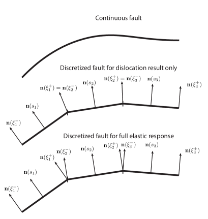
To calculate the full elastic response, we considered piecewise constant slip over straight elements of size $ds$. The stress is then evaluated at the center of the element (Rice, (1993); Cochard and Madariaga, (1994)) (see Fig. 6). The point connecting two adjacent element is called a node.

C.1 assumptions

We assume piecewise constant for the slip as well as for the tangential vector.

$$\begin{split}t^{i}(\xi)&=\sum_{j}t_{j}^{i}(H(\xi-s_{j}+\Delta s/2)-H(\xi-s_{j}-\Delta s/2))\\ \Delta u^{t}(\xi)&=\sum_{j}\Delta u^{t}_{j}(H(\xi-s_{j}+\Delta s/2)-H(\xi-s_{j}-\Delta s/2))\end{split}$$ (31)

If we try to apply the previous expressions on a node point $s_{k}+\Delta s/2$, the answer is not straight forward because the tangent is not define between two adjacent straight element. However, if one assume that the Heaviside function follows $H(0)=0.5$, we can find a solution:

$$\begin{split}t^{i}(s_{k}+\Delta s/2)&=\sum_{j}t_{j}^{i}(H(\xi-s_{j}+\Delta s/2)-H(\xi-s_{j}-\Delta s/2))\\ &=\frac{t_{k}^{i}+t_{k+1}^{i}}{2}\end{split}$$ (32)

The same holds for the slip at a node point.

C.2 Derivation

Let’s try to do the complete math for the whole problem:

$$\begin{split}&\int K(s,\xi)\frac{\partial}{\partial x^{t}}(t_{i}\Delta u^{t})=\int K(s,\xi)\left(\Delta u^{t}\frac{\partial}{\partial x^{t}}t^{i}+t^{i}\frac{\partial}{\partial x^{t}}\Delta u^{t}\right)\\ &\text{We include the discretisation}\\ &=\int K(s,\xi)\Delta u^{t}(\xi)\\ &\frac{\partial}{\partial x^{t}}\sum_{j}t_{j}^{i}(H(\xi-s_{j}+\Delta s/2)-H(\xi-s_{j}-\Delta s/2))+\\ &\int K(s,\xi)t^{i}(\xi)\\ &\frac{\partial}{\partial x^{t}}\sum_{j}\Delta u^{t}_{j}(H(\xi-s_{j}+\Delta s/2)-H(\xi-s_{j}-\Delta s/2))\\ &\text{We apply the derivative to the Heaviside function}\\ &=\int K(s,\xi)\Delta u^{t}(\xi)\sum_{j}t_{j}^{i}(\delta(\xi-s_{j}+\Delta s/2)-\delta(\xi-s_{j}-\Delta s/2))+\\ &\int K(s,\xi)t^{i}(\xi)\sum_{j}\Delta u_{j}^{t}(\delta(\xi-s_{j}+\Delta s/2)-\delta(\xi-s_{j}-\Delta s/2))\\ \end{split}$$ (33)

If we remove the integral and change the notation writting $s_{j}-\Delta s/2=\xi_{j}$ and $s_{j}+\Delta s/2=\xi_{j+1}$

$$\begin{split}&\sum_{j}t_{j}^{i}(K(s,\xi_{j})\Delta u^{t}(\xi_{j})-K(s,\xi_{j+1})\Delta u^{t}(\xi_{j+1}))+\\ &\sum_{j}\Delta u_{j}^{t}(K(s,\xi_{j})t^{i}(\xi_{j})-K(s,\xi_{j+1})t^{i}(\xi_{j+1}))\end{split}$$ (34)

Which is equivalent to

$$\begin{split}&\sum_{j}t_{j}^{i}\left(K(s,\xi_{j})\left[\frac{\Delta u^{t}_{j-1}+\Delta u^{t}_{j}}{2}\right]-K(s,\xi_{j+1})\left[\frac{\Delta u^{t}_{j}+\Delta u^{t}_{j+1}}{2}\right]\right)+\\ &\sum_{j}\Delta u_{j}^{t}\left(K(s,\xi_{j})\left[\frac{t^{i}_{j-1}+t^{i}_{j}}{2}\right]-K(s,\xi_{j+1})\left[\frac{t^{i}_{j}+t^{i}_{j+1}}{2}\right]\right)\\ &=\sum_{j}\Delta u_{j}^{t}K(s,\xi_{j})t^{i}_{j}-\Delta u_{j}^{t}K(s,\xi_{j+1})t^{i}_{j}\end{split}$$ (35)

The other terms are canceling each other:

$$\begin{split}t_{j}K(s,\xi_{j})\Delta u_{j-1}\\ -t_{j}K(s,\xi_{j})\Delta u_{j-1}\end{split}$$ (36)

We finally obtain:

$$\sigma_{ij}=\sum_{j}\Delta u_{j}^{t}K(s,\xi_{j})t^{i}_{j}-\Delta u_{j}^{t}K(s,\xi_{j+1})t^{i}_{j}$$ (37)

Which is the expression we used to get the full elastic response. When showing only the curvature effect, we just discretised the fault so that the tangential vector at a node point is the mean of the tangential vector of two adjacent elements (see Fig. 6).

References

- Aki and Richards, (2002) Aki, K. and Richards, P. G. (2002). Quantitative Seismology. University Science Books.
- Ando et al., (2017) Ando, R., Imanishi, K., Panayotopoulos, Y., and Kobayashi, T. (2017). Dynamic rupture propagation on geometrically complex fault with along-strike variation of fault maturity: insights from the 2014 northern nagano earthquake. Earth, Planets and Space, 69(1):130.
- Ando and Kaneko, (2018) Ando, R. and Kaneko, Y. (2018). Dynamic rupture simulation reproduces spontaneous multi-fault rupture and arrest during the 2016 mw 7.9 kaikoura earthquake. Geophys. Res. Lett.
- (4) Aochi, H., Fukuyama, E., and Matsu’ura, M. (2000a). Spontaneous rupture propagation on a non-planar fault in 3d elastic medium. Pure Appl. Geophys., 157:2003–2027.
- (5) Aochi, H., Fukuyama, E., and Matsu’ura, M. (2000b). Selectivity of spontaneous rupture propagation on a branched fault. Geophys. Res. Lett., 27:3635–3638.
- Bhat et al., (2004) Bhat, H. S., Dmowska, R., Rice, J. R., and Kame, N. (2004). Dynamic slip transfer from the denali to totschunda faults, alaska: Testing theory for fault branching. Bull. Seism. Soc. Am., 94:S202–S213.
- Bletery et al., (2016) Bletery, Q., Thomas, A. M., Rempel, A. W., Karlstrom, L., Sladen, A., and De Barros, L. (2016). Mega-earthquakes rupture flat megathrusts. Science, 354(6315):1027–1031.
- Bonnet, (1999) Bonnet, M. (1999). Boundary integral equation methods for solids and fluids, volume 34. Springer.
- Brodsky et al., (2011) Brodsky, E. E., Gilchrist, J. J., Sagy, A., and Collettini, C. (2011). Faults smooth gradually as a function of slip. Earth Planet. Sc. Lett., 302(1-2):185–193.
- Candela et al., (2009) Candela, T., Renard, F., Bouchon, M., Brouste, A., Marsan, D., Schmittbuhl, J., and Voisin, C. (2009). Characterization of fault roughness at various scales: Implications of three-dimensional high resolution topography measurements. In Mechanics, Structure and Evolution of Fault Zones, pages 1817–1851. Springer.
- Candela et al., (2012) Candela, T., Renard, F., Klinger, Y., Mair, K., Schmittbuhl, J., and Brodsky, E. E. (2012). Roughness of fault surfaces over nine decades of length scales. J. Geophys. Res., 117:B08409.
- Cochard and Madariaga, (1994) Cochard, A. and Madariaga, R. (1994). Dynamic faulting under rate-dependent friction. Pure Appl. Geophys., 142:419–445.
- Dunham et al., (2011) Dunham, E. M., Belanger, D., Cong, L., and Kozdon, J. E. (2011). Earthquake ruptures with strongly rate-weakening friction and off-fault plasticity, part 2: Nonplanar faults. Bull. Seism. Soc. Am., 101(5):2308–2322.
- Fang and Dunham, (2013) Fang, Z. and Dunham, E. M. (2013). Additional shear resistance from fault roughness and stress levels on geometrically complex faults. Journal of Geophysical Research: Solid Earth, 118(7):3642–3654.
- King and Nabelek, (1985) King, G. C. P. and Nabelek, J. (1985). The role of bends in faults in the initiation and termination of earthquake rupture. Science, 228:984–987.
- Koller et al., (1992) Koller, M. G., Bonnet, M., and Madariaga, R. (1992). Modelling of dynamical crack propagation using time-domain boundary integral equations. Wave Motion, 16(4):339–366.
- Lee and Bruhn, (1996) Lee, J.-J. and Bruhn, R. L. (1996). Structural anisotropy of normal fault surfaces. J. Struct. Geol., 18(8):1043–1059.
- Li and Liu, (2016) Li, D. and Liu, Y. (2016). Spatiotemporal evolution of slow slip events in a nonplanar fault model for northern cascadia subduction zone. J. Geophys. Res., 121(9):6828–6845.
- Martin et al., (1989) Martin, P., Rizzo, F., and Gonsalves, I. (1989). On hypersingular boundary integral equations for certain problems in mechanics. Mech. Res. Commun., 16(2):65–71.
- Oglesby, (2005) Oglesby, D. D. (2005). The dynamics of strike-slip step-overs with linking dip-slip faults. Bull. Seism. Soc. Am., 95(5):1604–1622.
- Poliakov et al., (2002) Poliakov, A. N. B., Dmowska, R., and Rice, J. R. (2002). Dynamic shear rupture interactions with fault bends and off-axis secondary faulting. J. Geophys. Res., 107(B11).
- Power et al., (1987) Power, W., Tullis, T., Brown, S., Boitnott, G., and Scholz, C. (1987). Roughness of natural fault surfaces. Geophys. Res. Lett., 14(1):29–32.
- Power and Tullis, (1991) Power, W. L. and Tullis, T. E. (1991). Euclidean and fractal models for the description of rock surface roughness. J. Geophys. Res., 96(B1):415–424.
- Renard et al., (2006) Renard, F., Voisin, C., Marsan, D., and Schmittbuhl, J. (2006). High resolution 3d laser scanner measurements of a strike-slip fault quantify its morphological anisotropy at all scales. Geophys. Res. Lett., 33(4).
- Rice, (1993) Rice, J. R. (1993). Spatio-temporal complexity of slip on a fault. J. Geophys. Res., 98(B6):9885–9907.
- Rice et al., (2005) Rice, J. R., Sammis, C. G., and Parsons, R. (2005). Off-fault secondary failure induced by a dynamic slip pulse. Bull. Seism. Soc. Am., 95(1):109–134.
- Romanet et al., (2018) Romanet, P., Bhat, H. S., Jolivet, R., and Madariaga, R. (2018). Fast and slow slip events emerge due to fault geometrical complexity. Geophys. Res. Lett., 45(10):4809–4819.
- Sagy et al., (2007) Sagy, A., Brodsky, E. E., and Axen, G. J. (2007). Evolution of fault-surface roughness with slip. Geology, 35(3):283–286.
- Sato et al., (2019) Sato, D. S., Romanet, P., and Ando, R. (2019). Paradox of modeling curved faults revisited with general non-hypersingular stress green’s functions.
- Sladek and Sladek, (1983) Sladek, V. and Sladek, J. (1983). Three-dimensional curved crack in an elastic body. International Journal of Solids and Structures, 19(5):425–436.
- Sladek and Sladek, (1984) Sladek, V. and Sladek, J. (1984). Transient elastodynamic three-dimensional problems in cracked bodies. Appl. Math. Modelling, 8(1):2–10.
- Tada et al., (2000) Tada, T., Fukuyama, E., and Madariaga, R. (2000). Non-hypersingular boundary integral equations for 3-d non-planar crack dynamics. Comput. Mech., 25(6):613–626.
- Tada and Yamashita, (1996) Tada, T. and Yamashita, T. (1996). The paradox of smooth and abrupt bends in two-dimensional in-plane shear-crack mechanics. Geophys. J. Int., 127(3).
- Tada and Yamashita, (1997) Tada, T. and Yamashita, T. (1997). Non-hypersingular boundary integral equations for two dimensional non-planar crack analysis. Geophys. J. Int., 130(2):269–282.
- Wesnousky, (2006) Wesnousky, S. G. (2006). Predicting the endpoints of earthquake ruptures. Nature, 444(7117):358–360.
- Wesnousky, (2008) Wesnousky, S. G. (2008). Displacement and geometrical characteristics of earthquake surface ruptures: Issues and implications for seismic-hazard analysis and the process of earthquake rupture. Bull. Seism. Soc. Am., 98(4):1609–1632.