On fixed-point, Krylov, and $2\times 2$ block
preconditioners for nonsymmetric problems

Abstract

The solution of matrices with $2\times 2$ block structure arises in numerous areas of computational mathematics, such as PDE discretizations based on mixed-finite element methods, constrained optimization problems, or the implicit or steady state treatment of any system of PDEs with multiple dependent variables. Often, these systems are solved iteratively using Krylov methods and some form of block preconditioner. Under the assumption that one diagonal block is inverted exactly, this paper proves a direct equivalence between convergence of $2\times 2$ block preconditioned Krylov or fixed-point iterations to a given tolerance, with convergence of the underlying preconditioned Schur-complement problem. In particular, results indicate that an effective Schur-complement preconditioner is a necessary and sufficient condition for rapid convergence of $2\times 2$ block-preconditioned GMRES, for arbitrary relative-residual stopping tolerances. A number of corollaries and related results give new insight into block preconditioning, such as the fact that approximate block-LDU or symmetric block-triangular preconditioners offer minimal reduction in iteration over block-triangular preconditioners, despite the additional computational cost. Theoretical results are verified numerically on a nonsymmetric steady linearized Navier–Stokes discretization, which also demonstrate that theory based on the assumption of an exact inverse of one diagonal block extends well to the more practical setting of inexact inverses.

65F08

1 Introduction

1.1 Problem

This paper considers block preconditioning and the corresponding convergence of fixed-point and Krylov methods applied to nonsymmetric systems of the form

(1) $$A\mathbf{x}=\mathbf{b},\qquad\mathbf{x},\mathbf{b}\in\mathbb{R}^{n\times n},\quad A\in\mathbb{R}^{n\times n},$$

where the matrix $A$ has a $2\times 2$ block structure,

(2) $$A=\begin{bmatrix}A_{11}&A_{12}\\ A_{21}&A_{22}\end{bmatrix}.$$

Such systems arise in numerous areas, including mixed finite element [7, 9, 17, 42], constraint optimization problems [34, 28, 11], and the solution of neutral particle transport [38]. More generally, the discretization of just about any systems of PDEs with multiple dependent variables can be expressed as a $2\times 2$ block operator by the grouping of variables into two sets. Although iterative methods for saddle-point problems, in which $A_{22}=\mathbf{0}$, have seen extensive research, in this paper we take a more general approach, making minimal assumptions on the submatrices of $A$.

The primary contribution of this paper is to prove a direct equivalence between the convergence of a block-preconditioned fixed-point or Krylov iteration applied to Eq. 1, with convergence of a similar method applied directly to a preconditioned Schur complement of $A$, where the Schur complements of $A$ are defined as $S_{11}\mathrel{\mathop{\mathchar 58\relax}}=A_{11}-A_{12}A_{22}^{-1}A_{21}$ and $S_{22}\mathrel{\mathop{\mathchar 58\relax}}=A_{22}-A_{21}A_{11}^{-1}A_{12}$. In particular, results in this paper prove that a good approximation to the Schur complement of the $2\times 2$ block matrix Eq. 2 is a necessary and sufficient condition for rapid convergence of preconditioned GMRES applied to Eq. 1, for arbitrary relative residual stopping tolerances.

The main assumption in derivations here is that at least one of $A_{11}$ or $A_{22}$ is non-singular and that the action of its inverse can be computed. Although in practice it is often not advantageous to solve one diagonal block to numerical precision every iteration, it is typically the case that the inverse of at least one diagonal block can be reliably computed using some form of iterative method, such as multigrid. The theory developed in this paper provides a guide for ensuring a convergent and practical preconditioner for Eq. 1. Once the iteration and convergence are well understood, the time to solution can be reduced by solving the diagonal block(s) to some tolerance. Numerical results in Section 4 demonstrate how ideas motivated by the theory, where one block is inverted exactly, extend to inexact preconditioners.

1.2 Previous work

For nonsymmetric $2\times 2$ block operators, most theoretical results in the literature are not necessarily indicative of practical performance. There is also a lack of distinction in the literature between a Krylov convergence result and a fixed-point convergence result, which we discuss in Section 2.

Theoretical results on block preconditioning generally fall in to one of two categories. First, are results based on the assumption that the inverse action of the Schur complement is available, and/or results that show an asymptotic equivalence between the preconditioned $2\times 2$ operator and the preconditioned Schur complement. It is shown in [16, 26] that GMRES (or other minimal residual methods) is guaranteed to converge in two or four iterations for a block-triangular or block-diagonal preconditioned system, respectively, when the diagonal blocks of the preconditioner consist of a Schur complement and the respective complementary block of $A$ ($A_{11}$ or $A_{22}$). However, computing the action of the Schur complement inverse is generally very expensive. In [4], it is shown that if the minimal polynomial of the preconditioned Schur complement is degree $k$, then the minimal polynomial of the preconditioned $2\times 2$ system is at most degree $k+1$. Although this does not require the action and inverse of the Schur complement, it is almost never the case that GMRES is iterated until the true minimal polynomial is achieved. As a consequence, the minimal polynomial equivalence also does not provide practical information on convergence of the $2\times 2$ system, as demonstrated in the following example.

Example 1.1.

Define two matrices $A_{1},A_{2}\in\mathbb{R}^{1000\times 1000}$,

$$A_{1}\mathrel{\mathop{\mathchar 58\relax}}=\begin{bmatrix}I_{500}&\mathbf{0}\\ \mathbf{0}&D_{1}\end{bmatrix},\hskip 21.52771ptA_{2}\mathrel{\mathop{\mathchar 58\relax}}=\begin{bmatrix}I_{500}&\mathbf{0}\\ \mathbf{0}&D_{2}\end{bmatrix},$$

where $D_{1}\in\mathbb{R}^{500\times 500}$ is tridiagonal with stencil $[-1,2,-1]$ and $D_{2}\in\mathbb{R}^{500\times 500}$ is tridiagonal with stencil $[-1,2.0025,-1]$. Note that the minimal polynomials of $A_{1}$ and $A_{2}$ in the $\ell^{2}$-norm have degree at most $k=501$. Figure 1(a) shows results from applying GMRES with no restarts to $A_{1}$ and $A_{2}$, with right-hand side $\mathbf{b}=(1,2,...,1000)^{T}/1000$. Note that neither operator reaches exact convergence in the first 500 iterations, indicating that the minimal polynomial in both cases is degree $k=501$. However, despite having the same degree minimal polynomial (which is less than the size of the matrix), at iteration 250, $A_{2}$ has reached a residual of $\mathinner{\!\left\lVert\mathbf{r}\right\rVert}\approx 10^{-5}$, while $A_{1}$ still has residual $\mathinner{\!\left\lVert\mathbf{r}\right\rVert}>1$.

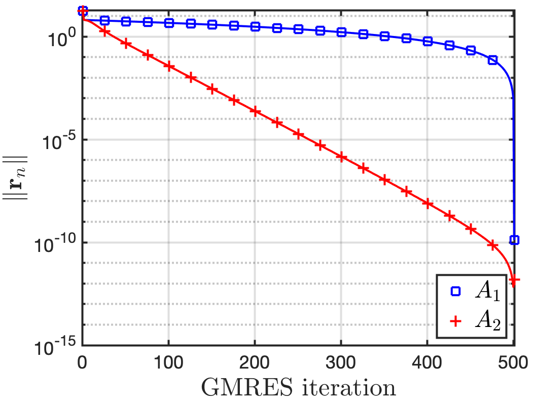
(a) Minimal polynomial does not necessarily provide practical information on convergence of a $2\times 2$ system (Example 1.1).

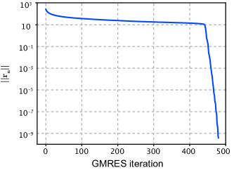
(b) Eigenvalues do not necessarily provide practical information on convergence of a $2\times 2$ system (Example 1.2).

Second, many papers have used eigenvalue analyses in an attempt to provide more practical information on convergence. In the symmetric setting, this has proven effective (see, for example, [27]). Spectral analyses have also been done for various nonsymmetric $2\times 2$ block matrices and preconditioners [12, 17, 3, 4, 19, 35] and eigenvectors for preconditioned operators derived in [29]. However, eigenvalue analyses are asymptotic, guaranteeing eventual convergence but, in the nonsymmetric setting, giving no guarantee of practical performance. In certain cases, a nonsymmetric operator is symmetric in a non-standard inner product, and some of papers have looked at block preconditioning in modified norms [30, 41, 31, 25] that yield self-adjointness. Nevertheless, there are many nonsymmetric problems that are not easily symmetrized and/or where eigenvalues provide little to no practical information on convergence of iterative methods. The following provides one such example in the discretization of differential operators. A formal analysis as in [15, 40] proves that for any set of eigenvalues, there is a matrix such that GMRES converges arbitrarily slowly.

Example 1.2.

Consider an upwind discontinuous Galerkin (DG) discretization of linear advection with Dirichlet inflow boundaries [8] and a velocity field $\mathbf{b}(x,y)\mathrel{\mathop{\mathchar 58\relax}}=(\cos(\pi y)^{2},\cos(\pi x)^{2})$ (see Figure 5a in [23]); more generally, similar results hold for any velocity field with no cycles). In the appropriate ordering, the resulting matrix is block triangular, where “block” refers to the DG element blocks. Then, if we apply block-diagonal (Jacobi) preconditioning, the spectrum of the preconditioned operator is given by $\sigma(M^{-1}A)=\{1\}$, and the spectrum of the fixed-point iteration is given by $\sigma(I-M^{-1}A)=\{0\}$. Despite all zero eigenvalues, block-Jacobi preconditioned fixed-point or GMRES iterations on such a matrix can converge arbitrarily slowly, until the degree of nilpotency is reached and exact convergence is immediately obtained. Figure 1(b) shows convergence of DG block-Jacobi preconditioned GMRES applied to 2d linear transport, with $200\times 200$ finite elements. Convergence occurs very rapidly at around 450 iterations (without restart), approximately equal to the diameter of the mesh (as expected [23]).

This is not the first work to recognize that eigenvalue analyses of nonsymmetric block preconditioners may be of limited practical use. Norm and field-of-values equivalence are known to provide more accurate measures of convergence for nonsymmetric operators, used as early as [22], and applied recently for specific problems in [6, 18, 20, 21]. Here, we stay even more general, focusing directly on the relation between polynomials of a general preconditioned $2\times 2$ system and the preconditioned Schur complement.

1.3 Overview of results

The paper proceeds as follows. Section 2 formally introduces various block preconditioners, considers the distinction between fixed-point and Krylov methods, and derives some relationships on polynomials of the preconditioned operators that define Krylov and fixed-point iterations. Proofs and formal statements of results are provided in Section 3, and numerical results are examined in Section 4, with a discussion on the practical implications of theory developed here. We conclude in Section 5.

Because the formal derivations are lengthy, the following list provides a brief overview of theoretical contributions of this paper.

• Fixed-point and minimal residual Krylov iterations preconditioned with a $2\times 2$ block-triangular, block-Jacobi, or approximate block-LDU preconditioner converge to a given tolerance $C\rho$ after $n$ iterations if and only if an equivalent method applied to the underlying preconditioned Schur complement converges to tolerance $\rho$ after $n$ iterations, for constant $C$ (Section 3). Such results do not hold for general block-diagonal preconditioners [39].

• A symmetric block-triangular or approximate block-LDU preconditioner offers little to no improvement in convergence over block-triangular preconditioners, when one diagonal block is inverted exactly (Section 2.1.1). Numerical results demonstrate the same behaviour for inexact inverses, suggesting that symmetric block-triangular or block-LDU preconditioners are probably not worth the added computational cost in practice.

• The worst-case number of iterations for a block-Jacobi preconditioner to converge to a given tolerance $\rho$ is twice the number of iterations for a block-triangular preconditioner to converge to $C\rho$, for some constant factor $C$ (Section 3.3). Numerical results suggest that for non-saddle point problems (nonzero (2,2)-block), this double in iteration count is not due to the staircasing effect introduced in [14] for saddle-point problems.

• With an exact Schur-complement inverse, a fixed-point iteration with a block-triangular preconditioner converges in two iterations, while a fixed-point iteration with a block-diagonal preconditioner does not converge (Section 2).

2 Block preconditioners

This paper considers $2\times 2$ block preconditioners, where one diagonal block is inverted exactly, and the other is some approximation to the Schur complement.

We consider four different kinds of block preconditioners: block diagonal, block upper triangular, block lower triangular, and block LDU, denoted $D$, $U$, $L$, and $M$, respectively. If the preconditioners have no subscript, this implies the diagonal blocks of the preconditioners are the diagonal blocks of $A$. If one of the diagonal blocks is some approximation to the Schur complement $S_{kk}$, $k\in\{1,2\}$, then a $11$- or $22$- subscript denotes in which block the approximation is used. For example, with a Schur-complement approximation in the $(1,1)$-block, preconditioners take the forms

(3) $$L_{11} \mathrel{\mathop{\mathchar 58\relax}}=\begin{bmatrix}\widehat{S}_{11}&\mathbf{0}\\ A_{21}&A_{22}\end{bmatrix}, U_{11} \mathrel{\mathop{\mathchar 58\relax}}=\begin{bmatrix}\widehat{S}_{11}&A_{12}\\ \mathbf{0}&A_{22}\end{bmatrix},$$

$$D_{11} \mathrel{\mathop{\mathchar 58\relax}}=\begin{bmatrix}\widehat{S}_{11}&\mathbf{0}\\ \mathbf{0}&A_{22}\end{bmatrix}, M_{11} \mathrel{\mathop{\mathchar 58\relax}}=\begin{bmatrix}I&A_{12}A_{22}^{-1}\\ \mathbf{0}&I\end{bmatrix}\begin{bmatrix}\widehat{S}_{11}&\mathbf{0}\\ \mathbf{0}&A_{22}\end{bmatrix}\begin{bmatrix}I&\mathbf{0}\\ A_{22}^{-1}A_{21}&I\end{bmatrix}.$$

The block-diagonal, block upper-triangular, and block lower-triangular preconditioners with a Schur-complement approximation in the $(2,2)$-block take an analogous form, with $\widehat{S}_{11}\mapsto A_{11}$ and $A_{22}\mapsto\widehat{S}_{22}$, and the approximate block LDU preconditioner $M_{22}$ is given by

(4) $$M_{22}\mathrel{\mathop{\mathchar 58\relax}}=\begin{bmatrix}I&\mathbf{0}\\ A_{21}A_{11}^{-1}&I\end{bmatrix}\begin{bmatrix}A_{11}&\mathbf{0}\\ \mathbf{0}&\widehat{S}_{22}\end{bmatrix}\begin{bmatrix}I&A_{11}^{-1}A_{12}\\ \mathbf{0}&I\end{bmatrix}.$$

Most results here regarding block-diagonal preconditiong are for the specific case of block Jacobi, where $D_{11}=D_{22}=D$ is the block diagonal of $A$.

Preconditioners are typically used in conjunction with either a fixed-point iteration or Krylov subspace method to approximately solve a linear system Eq. 1. Krylov methods approximate the solution to linear systems by constructing a Krylov space of vectors and minimizing the error of the approximate solution over this space, in a given norm. The Krylov space is formed as powers of the preconditioned operator applied to the initial residual. For linear system $A\mathbf{x}=\mathbf{b}$, (left) preconditioner $M^{-1}$, and initial residual $\mathbf{r}_{0}$, the $d$th Krylov space takes the form

$$\mathcal{K}_{d}\mathrel{\mathop{\mathchar 58\relax}}=\mathinner{\left\{\mathbf{r}_{0},M^{-1}A\mathbf{r}_{0},...,(M^{-1}A)^{d-1}\mathbf{r}_{0}\right\}}.$$

Minimizing over this space is thus equivalent to constructing a minimizing polynomial $p(M^{-1}A)\mathbf{r}_{0}$, which is optimal in a given norm. This optimality can be in the operator norm (that is, including a $\sup_{\mathbf{r}_{0}\neq\mathbf{0}}$) for a worst-case convergence over all initial guesses and right-hand sides, or optimal for a specific initial residual. Examples include CG, which minimizes error in the $A$-norm, MINRES, which minimizes error in the $AM^{-1}A$-norm [1], left-preconditioned GMRES, which minimizes error in the $(M^{-1}A)^{*}(M^{-1}A)$-norm, or right-preconditioned GMRES, which minimizes error in the $A^{*}A$-norm. Note that error in the $A^{*}A$-norm is equivalent to residual in the $\ell^{2}$-norm, which is how minimal-residual methods are typically presented. Fixed-point iterations also correspond to polynomials of the preconditioned operator, but they are not necessarily optimal in a specific norm.

Analysis in this paper is focused on polynomials of block-preconditioned operators, particularly deriving upper and lower bounds on minimizing Krylov polynomials of a fixed degree. Section 2.1 begins by considering fixed-point iterations and the corresponding matrix polynomials in the nonsymmetric setting, and discusses important differences between the various preconditioners in Eq. 3 and Eq. 4. Section 2.2 then examines general polynomials of the preconditioned operator, developing the theoretical framework used in Section 3 to analyze convergence of block-preconditioned Krylov methods. Due to the equivalence of a Krylov method and a minimizing polynomial of the preconditioned operator, we refer to, for example, GMRES and a minimizing polynomial of $p(M^{-1}A)$ in the $\ell^{2}$-norm, interchangeably.

2.1 Observations on fixed-point iterations

For some approximate inverse $P$ to linear operator $A$, error propagation of a fixed-point iteration takes the form $\mathcal{E}\mathrel{\mathop{\mathchar 58\relax}}=I-P^{-1}A$ and residual propagation takes the form $\mathcal{R}\mathrel{\mathop{\mathchar 58\relax}}=A\mathcal{E}^{-1}A=I-AP^{-1}$. Define

(5) $$\begin{split}\mathcal{E}_{{11}}&\mathrel{\mathop{\mathchar 58\relax}}=I-\widehat{S}_{11}^{-1}S_{11},\hskip 21.52771pt\mathcal{R}_{{11}}\mathrel{\mathop{\mathchar 58\relax}}=I-S_{11}\widehat{S}_{11}^{-1},\\ \mathcal{E}_{{22}}&\mathrel{\mathop{\mathchar 58\relax}}=I-\widehat{S}_{22}^{-1}S_{22},\hskip 21.52771pt\mathcal{R}_{{22}}\mathrel{\mathop{\mathchar 58\relax}}=I-S_{22}\widehat{S}_{22}^{-1}.\end{split}$$

Consider first block-triangular and approximate block-LDU preconditioners. Powers of fixed-point error and residual propagation with these block preconditioners take the following forms:

(6) $$\begin{split}&(I-L_{11}^{-1}A)^{d}=\begin{bmatrix}I\\ -A_{22}^{-1}A_{21}\end{bmatrix}\mathcal{E}_{{11}}^{d-1}\begin{bmatrix}I-\widehat{S}_{11}^{-1}A_{11}&-\widehat{S}_{11}^{-1}A_{12}\end{bmatrix},\\ &(I-AL_{22}^{-1})^{d}=\begin{bmatrix}-A_{12}\widehat{S}_{22}^{-1}\\ I-A_{22}\widehat{S}_{22}^{-1}\end{bmatrix}\mathcal{R}_{{22}}^{d-1}\begin{bmatrix}-A_{21}A_{11}^{-1}&I\end{bmatrix},\\ &(I-AU_{11}^{-1})^{d}=\begin{bmatrix}I-A_{11}\widehat{S}_{11}^{-1}\\ -A_{21}\widehat{S}_{11}^{-1}\end{bmatrix}\mathcal{R}_{{11}}^{d-1}\begin{bmatrix}I&-A_{12}{A}_{22}^{-1}\end{bmatrix},\\ &(I-U_{22}^{-1}A)^{d}=\begin{bmatrix}-A_{11}^{-1}A_{12}\\ I\end{bmatrix}\mathcal{E}_{{22}}^{d-1}\begin{bmatrix}-\widehat{S}_{22}^{-1}A_{21}&I-\widehat{S}_{22}^{-1}A_{22}\end{bmatrix},\end{split}$$

$$(I-AL_{11}^{-1})^{d} =\begin{bmatrix}\mathcal{R}_{{11}}^{p}&-\mathcal{R}_{{11}}^{d-1}A_{12}A_{22}^{-1}\\ \mathbf{0}&\mathbf{0}\end{bmatrix},\hskip 12.91663pt(I-L_{22}^{-1}A)^{d}=\begin{bmatrix}\mathbf{0}&-A_{11}^{-1}A_{12}\mathcal{E}_{{22}}^{d-1}\\ \mathbf{0}&\mathcal{E}_{{22}}^{d}\end{bmatrix}$$

$$(I-AU_{22}^{-1})^{d} =\begin{bmatrix}\mathbf{0}&\mathbf{0}\\ -\mathcal{R}_{{22}}^{d-1}A_{21}A_{11}^{-1}&\mathcal{R}_{{22}}^{d}\end{bmatrix},\hskip 12.91663pt(I-U_{11}^{-1}A)^{d}=\begin{bmatrix}\mathcal{E}_{{11}}^{d}&\mathbf{0}\\ -A_{22}^{-1}A_{21}\mathcal{E}_{{11}}^{d-1}&\mathbf{0}\end{bmatrix},$$

$$(I-M_{11}^{-1}A)^{d} =\begin{bmatrix}\mathcal{E}_{{11}}^{d}&\mathbf{0}\\ -A_{22}^{-1}A_{21}\mathcal{E}_{{11}}^{d}&\mathbf{0}\end{bmatrix},\hskip 30.1388pt(I-AM_{11}^{-1})^{d}=\begin{bmatrix}\mathcal{R}_{{11}}^{d}&-\mathcal{R}_{{11}}^{d}A_{12}A_{22}^{-1}\\ \mathbf{0}&\mathbf{0}\end{bmatrix},$$

$$(I-M_{22}^{-1}A)^{d} =\begin{bmatrix}\mathbf{0}&-A_{11}^{-1}A_{12}\mathcal{E}_{{22}}^{d}\\ \mathbf{0}&\mathcal{E}_{{22}}^{d}\end{bmatrix},\hskip 30.1388pt(I-AM_{22}^{-1})^{d}=\begin{bmatrix}\mathbf{0}&\mathbf{0}\\ -\mathcal{R}_{{22}}^{d}A_{21}A_{11}^{-1}&\mathcal{R}_{{22}}^{d}\end{bmatrix}.$$

Let $\mathinner{\!\left\lVert\cdot\right\rVert}$ be a given norm on $A$ and $\mathinner{\!\left\lVert\cdot\right\rVert}_{c}$ be a given norm on the Schur-complement problem. Note that any of the above fixed-point iterations is convergent in $\mathinner{\!\left\lVert\cdot\right\rVert}$ for all initial error or residual, if and only if the corresponding Schur-complement fixed-point iteration in Eq. 5 is convergent in $\mathinner{\!\left\lVert\cdot\right\rVert}_{c}$. Moreover, it is well-known that for block-triangular preconditioners with an exact Schur complement, minimal residual Krylov methods converge in two iterations [16, 26]. However, convergence in two iterations actually follows from fixed-point convergence rather than Krylov iterations.

Proposition 2.1 (Block triangular-preconditioners with Schur complement).

If $\widehat{{S}}_{kk}={S}_{kk}$, for $k\in\{1,2\}$, then fixed-point iteration with a (left or right) block upper or block lower-triangular preconditioner converges in two iterations.

Proof 2.2.

The proof follows by noting that if $\widehat{{S}}_{kk}={S}_{kk}$, for $k\in\{1,2\}$, then all terms defined in (5) are zero.

Now consider block-diagonal preconditioners. Then,

$$I-D_{11}^{-1}A =\begin{bmatrix}I-\widehat{S}_{11}^{-1}A_{11}&-\widehat{S}_{11}^{-1}A_{12}\\ -{A}_{22}^{-1}A_{21}&\mathbf{0}\end{bmatrix},\hskip 12.91663ptI-AD_{11}^{-1}=\begin{bmatrix}I-A_{11}\widehat{S}_{11}^{-1}&-A_{12}{A}_{22}^{-1}\\ -A_{21}\widehat{S}_{11}^{-1}&\mathbf{0}\end{bmatrix},$$

$$I-D_{22}^{-1}A =\begin{bmatrix}\mathbf{0}&-A_{11}^{-1}A_{12}\\ -\widehat{S}_{22}^{-1}A_{21}&I-\widehat{S}_{22}^{-1}A_{22}\end{bmatrix},\hskip 13.99301ptI-AD_{22}^{-1}=\begin{bmatrix}\mathbf{0}&-A_{12}\widehat{S}_{22}^{-1}\\ -A_{21}A_{11}^{-1}&I-A_{22}\widehat{S}_{22}^{-1}\end{bmatrix}.$$

If we simplify to block Jacobi (that is, $\widehat{S}_{kk}\mathrel{\mathop{\mathchar 58\relax}}=A_{kk}$ for $k\in\{1,2\}$), both diagonal blocks are zero, and a closed form for powers of block-diagonal preconditioners can be obtained for an arbitrary number of fixed-point iterations,

(7) $$\begin{split}(I-D^{-1}A)^{2d}&=\begin{bmatrix}A_{11}^{-1}A_{12}A_{22}^{-1}A_{21}&\mathbf{0}\\ \mathbf{0}&A_{22}^{-1}A_{21}A_{11}^{-1}A_{12}\end{bmatrix}^{d},\\ (I-AD^{-1})^{2d}&=\begin{bmatrix}A_{12}A_{22}^{-1}A_{21}A_{11}^{-1}&\mathbf{0}\\ \mathbf{0}&A_{21}A_{11}^{-1}A_{12}A_{22}^{-1}\end{bmatrix}^{d}.\end{split}$$

Noting that if $\widehat{S}_{11}\mathrel{\mathop{\mathchar 58\relax}}=A_{11}$ and $\widehat{S}_{22}\mathrel{\mathop{\mathchar 58\relax}}=A_{22}$ in Eq. 5, then

$$(I-D^{-1}A)^{2d}=\begin{bmatrix}\mathcal{E}_{{11}}&\mathbf{0}\\ \mathbf{0}&\mathcal{E}_{{22}}\end{bmatrix}^{d},\qquad(I-AD^{-1})^{2d}=\begin{bmatrix}\mathcal{R}_{{11}}&\mathbf{0}\\ \mathbf{0}&\mathcal{R}_{{22}}\end{bmatrix}^{d}.$$

It follows that block Jacobi converges if and only if block upper- and lower-triangular preconditioners, with diagonal blocks given by $A_{11}$ and $A_{22}$, both converge. Furthermore, the expected number of iterations of block Jacobi to converge to a given tolerance are approximately double that of the equivalent block-triangular preconditioning, give or take some independent constant factor (e.g., $A_{11}^{-1}A_{12}$) from the fixed-point operators. A similar result is later shown for preconditioning Krylov methods with block Jacobi (see Theorem 3.10). This relation of twice as many iterations for Jacobi/block-diagonal preconditioning has been noted or observed a number of times, perhaps originally in [14] where MINRES/GMRES are proven to stall every other iteration on saddle-point problems.

Remark 2.3 (Non-convergent block-diagonal fixed-point).

As mentioned above, fixed-point iteration converges in two iterations for a block-triangular preconditioner if the Schur complement is inverted exactly. However, the same does not hold for block Jacobi. Let $D_{22}$ be a block diagonal preconditioner with $\widehat{S}_{22}\mathrel{\mathop{\mathchar 58\relax}}=S_{22}$. In the case of a saddle-point matrix, say $B$, where $B_{22}=\mathbf{0}$,

$$(I-D_{22}^{-1}B)^{3d} =\begin{bmatrix}\mathbf{0}&-B_{11}^{-1}B_{12}\\ -S_{22}^{-1}B_{21}&I\end{bmatrix}^{3d}=(-1)^{d}\begin{bmatrix}-B_{11}^{-1}B_{12}S_{22}^{-1}B_{21}&\mathbf{0}\\ \mathbf{0}&I\end{bmatrix},$$

where $S_{22}\mathrel{\mathop{\mathchar 58\relax}}=-B_{21}B_{11}^{-1}B_{12}$. Here we see the interesting property that as we continue to iterate, error-propagation of block-diagonal preconditioning does not converge or diverge. In fact, $(I-D_{22}^{-1}B)^{3d}$ is actually a periodic point of period two under the matrix-valued mapping $(I-D_{22}^{-1}B)^{3}$, for $d\geq 1$. The general $2\times 2$ case is more complicated and does not appear to have such a property. However, expanding to up to four powers gave no indication that it would result in a convergent fixed-point iteration, as it does with GMRES acceleration [16].

Remark 2.4 (Non-optimal block-diagonal Krylov).

For $2\times 2$ systems with nonzero diagonal blocks, block-diagonal preconditioning of minimal-residual methods with an exact Schur complement does not necessarily converge in a fixed number of iterations, in contrast to block-triangular preconditioners or block-diagonal preconditioners for matrices with a zero (2,2) block (for example, see [2, 36] for the symmetric case, and [39] for a complete eigenvalue decomposition of general block-diagonal preconditioned operators, with preconditioning based on either the diagonal blocks or an exact Schur complement).

2.1.1 Symmetric block-triangular preconditioners

The benefit of Jacobi or block-diagonal preconditioning for SPD matrices is that they are also SPD, which permits the use of three-term recursion relations like conjugate gradient (CG) and MINRES, whereas block upper- or lower-triangular preconditioners are not applicable. Approximate block-LDU preconditioners offer one symmetric option. Another option that might be considered, particularly by those that work in iterative or multigrid methods, is a symmetric triangular iteration, consisting of a block-upper triangular iteration followed by a block-lower triangular iteration (or vice versa), akin to a symmetric (block) Gauss–Seidel sweep. Interestingly, this does not appear to be an effective choice. Consider a symmetric block-triangular preconditioner with approximate Schur complement in the (2,2)-block. The preconditioner can take two forms, depending on whether the lower or upper iteration is done first. For example,

$$(I-L_{22}^{-1}A)(I-U_{22}^{-1}A) =I-L_{22}^{-1}(L_{22}+U_{22}+A)U_{22}^{-1}A,$$

$$(I-U_{22}^{-1}A)(I-L_{22}^{-1}A) =I-U_{22}^{-1}(L_{22}+U_{22}+A)L_{22}^{-1}A.$$

Define $\mathcal{H}^{-1}_{22}\mathrel{\mathop{\mathchar 58\relax}}=L_{22}^{-1}(L_{22}+U_{22}+A)U_{22}^{-1}$ and $\mathcal{G}^{-1}_{22}\mathrel{\mathop{\mathchar 58\relax}}=U_{22}^{-1}(L_{22}+U_{22}+A)L_{22}^{-1}$, corresponding to upper-lower and lower-upper, symmetric preconditioners respectively. Expanding in block form, we see that preconditioners associated with a symmetric block-triangular iteration are given by

$$\mathcal{H}^{-1}_{22} \mathrel{\mathop{\mathchar 58\relax}}=\begin{bmatrix}I&\mathbf{0}\\ -\widehat{S}_{22}^{-1}A_{21}&I\end{bmatrix}\begin{bmatrix}A_{11}^{-1}&\mathbf{0}\\ \mathbf{0}&2\widehat{S}_{22}^{-1}-\widehat{S}_{22}^{-1}A_{22}\widehat{S}_{22}^{-1}\end{bmatrix}\begin{bmatrix}I&-A_{12}\widehat{S}_{22}^{-1}\\ \mathbf{0}&I\end{bmatrix},$$

$$\mathcal{G}^{-1}_{22} \mathrel{\mathop{\mathchar 58\relax}}=\begin{bmatrix}I&-A_{11}^{-1}A_{12}\\ \mathbf{0}&I\end{bmatrix}\begin{bmatrix}A_{11}^{-1}&\mathbf{0}\\ \mathbf{0}&2\widehat{S}_{22}^{-1}-\widehat{S}_{22}^{-1}A_{22}\widehat{S}_{22}^{-1}\end{bmatrix}\begin{bmatrix}I&\mathbf{0}\\ -A_{21}A_{11}^{-1}&I\end{bmatrix}.$$

Notice that each of these preconditioners can be expressed as a certain block-LDU type preconditioner, however, it is not clear that either would be as good as or a better preconditioner than block LDU. In the simplest (and also fairly common) case that $\widehat{S}_{22}=A_{22}$, then $\mathcal{H}_{22}^{-1}$ and $\mathcal{G}_{22}^{-1}$ are exactly equivalent to the two variants of block-LDU preconditioning in Eq. 3 and Eq. 4, respectively, with diagonal blocks used to approximate the Schur complement. As we will see in Section 2.2.3, this is also formally equivalent to a block-triangular preconditioner.

Adding an approximation to the Schur complement in the (2,2)-block, $\mathcal{G}_{22}^{-1}$, is equivalent to block-LDU preconditioning with Schur-complement approximation in the (2,2)-block, except that now we approximate $S_{22}^{-1}$ with the operator $2\widehat{S}_{22}^{-1}-\widehat{S}_{22}^{-1}A_{22}\widehat{S}_{22}^{-1}$, as opposed to $\widehat{S}_{22}^{-1}$ in block-LDU preconditioning Eq. 4. It is not clear if such an approach would ever be beneficial over standard LDU, although it is possible one can construct such a problem. For $\widehat{S}_{22}\neq A_{22}$, it is even less clear that $\mathcal{H}_{22}^{-1}$ would make a good or better preconditioner compared with LDU or block triangular. Analogous things can be said about Schur-complement approximations in the (1,1)-block. Numerical results in Section 4 confirm these observations, where symmetric block-triangular preconditioners offer at best a marginal reduction in total iteration count over block upper- or lower- triangular preconditioners, and sometimes observe worse convergence, at the expense of several additional (approximate) inverses.

2.2 Krylov and polynomials of the preconditioned matrix

This section begins by considering polynomials applied to the approximate block-LDU and block-triangular preconditioned operators in Section 2.2.1 and Section 2.2.2, respectively (the block-diagonal preconditioner is discussed in Section 3.3). These results are used in Section 2.2.3 to construct a norm in which fixed-point or Krylov iterations applied to approximate block-LDU or block-triangular preconditioned operators are equivalent to the preconditioned Schur complement. Section 2.2.4 uses this equivalence to motivate the key tool used in proofs provided in Section 3.

2.2.1 Approximate block-LDU preconditioner

In this section we apply a polynomial to the block-LDU preconditioned operator. For an approximate block-LDU preconditioner with approximate Schur complement in the $(2,2)$-block,

(8) $$M_{22}^{-1}A=\begin{bmatrix}I&-A_{11}^{-1}A_{12}\\ \mathbf{0}&I\end{bmatrix}\begin{bmatrix}I&\mathbf{0}\\ \mathbf{0}&\widehat{S}_{22}^{-1}S_{22}\end{bmatrix}\begin{bmatrix}I&A_{11}^{-1}A_{12}\\ \mathbf{0}&I\end{bmatrix}\mathrel{\mathop{\mathchar 58\relax}}=P_{1}\begin{bmatrix}I&\mathbf{0}\\ \mathbf{0}&\widehat{S}_{22}^{-1}S_{22}\end{bmatrix}P_{1}^{-1}.$$

The three-term formula reveals the change of basis matrix, $P_{1}$, between the LDU-preconditioned operator and the Schur-complement problem. This allows us to express polynomials $p$ of the preconditioned operator as a change of basis applied to the polynomial of the preconditioned Schur complement and the identity,

(9) $$\begin{split}p(M_{22}^{-1}A)&=\begin{bmatrix}I&-A_{11}^{-1}A_{12}\\ \mathbf{0}&I\end{bmatrix}\begin{bmatrix}p(I)&\mathbf{0}\\ \mathbf{0}&p(\widehat{S}_{22}^{-1}S_{22})\end{bmatrix}\begin{bmatrix}I&A_{11}^{-1}A_{12}\\ \mathbf{0}&I\end{bmatrix}\\ &=\begin{bmatrix}p(I)&A_{11}^{-1}A_{12}\left(p(I)-p(\widehat{S}_{22}^{-1}S_{22})\right)\\ \mathbf{0}&p(\widehat{S}_{22}^{-1}S_{22})\end{bmatrix}.\end{split}$$

Using right preconditioning, the polynomial takes the form

$$p(AM_{22}^{-1}) =\begin{bmatrix}I&\mathbf{0}\\ A_{21}A_{11}^{-1}&I\end{bmatrix}\begin{bmatrix}p(I)&\mathbf{0}\\ \mathbf{0}&p(S_{22}\widehat{S}_{22}^{-1})\end{bmatrix}\begin{bmatrix}I&\mathbf{0}\\ -A_{21}A_{11}^{-1}&I\end{bmatrix}$$

$$=\begin{bmatrix}p(I)&\mathbf{0}\\ \left(p(I)-p(S_{22}\widehat{S}_{22}^{-1})\right)A_{21}A_{11}^{-1}&p(S_{22}\widehat{S}_{22}^{-1})\end{bmatrix}.$$

Similarly, polynomials of the left and right preconditioned operator by a block LDU with approximate Schur complement in the $(1,1)$-block take the form

(10) $$\begin{split}p(M_{11}^{-1}A)&=\begin{bmatrix}p(\widehat{S}_{11}^{-1}S_{11})&\mathbf{0}\\ A_{22}^{-1}A_{21}\left(p(I)-p(\widehat{S}_{11}^{-1}S_{11})\right)&p(I)\end{bmatrix},\\ p(AM_{11}^{-1})&=\begin{bmatrix}p(S_{11}\widehat{S}_{11}^{-1})&\left(p(I)-p(S_{11}\widehat{S}_{11}^{-1})\right)A_{12}A_{22}^{-1}\\ \mathbf{0}&p(I)\end{bmatrix}.\end{split}$$

2.2.2 Block-triangular preconditioner

We now consider polynomials of a block-triangular preconditioned operator. Notice that error- and residual-propagation operators for four of the block-triangular preconditioners in Eq. 6 take a convenient form, with two zero blocks in the $2\times 2$ matrix. We focus on these operators in particular, looking at the left and right preconditioned operators

$$U_{11}^{-1}A =\begin{bmatrix}\widehat{S}_{11}^{-1}S_{11}&\mathbf{0}\\ A_{22}^{-1}A_{21}&I\end{bmatrix},\hskip 21.52771ptAL_{11}^{-1}=\begin{bmatrix}S_{11}\widehat{S}_{11}^{-1}&A_{12}A_{22}^{-1}\\ \mathbf{0}&I\end{bmatrix},$$

$$L_{22}^{-1}A =\begin{bmatrix}I&A_{11}^{-1}A_{12}\\ \mathbf{0}&\widehat{S}_{22}^{-1}S_{22}\end{bmatrix},\hskip 21.52771ptAU_{22}^{-1}=\begin{bmatrix}I&\mathbf{0}\\ A_{21}A_{11}^{-1}&S_{22}\widehat{S}_{22}^{-1}\end{bmatrix}.$$

These block triangular operators are easy to raise to powers; for example,

(11) $$(U_{11}^{-1}A)^{d} =\begin{bmatrix}(\widehat{S}_{11}^{-1}S_{11})^{d}&\mathbf{0}\\ A_{22}^{-1}A_{21}\sum_{\ell=0}^{d-1}(\widehat{S}_{11}^{-1}S_{11})^{\ell}&I\end{bmatrix},$$

with similar block structures for $(AL_{11}^{-1})^{d}$, $(L_{22}^{-1}A)^{d}$, and $(AU_{22}^{-1})^{d}$.

Now consider some polynomial $p(t)$ of degree $d$ with coefficients $\{\alpha_{i}\}$ applied to the preconditioned operator. Diagonal blocks are given by the polynomial directly applied to the diagonal blocks, in this case $p(\widehat{S}_{11}^{-1}S_{11})$ and $p(I)$. One off-diagonal block will be zero and the other (for $p(U_{11}^{-1}A)$) takes the form $A_{22}^{-1}A_{21}F$, where

(12) $$F\mathrel{\mathop{\mathchar 58\relax}}=\sum_{i=1}^{d}\alpha_{i}\sum_{\ell=0}^{i-1}(\widehat{S}_{11}^{-1}S_{11})^{\ell}.$$

Assume that $p(t)$ is a consistent polynomial, $p(0)=1$, as is the case in Krylov or fixed-point iterations. Then $\alpha_{0}=1$, and

(13) $$\begin{split}F(I-\widehat{S}_{11}^{-1}S_{11})&=\sum_{i=1}^{d}\alpha_{i}I-\sum_{i=1}^{d}\alpha_{i}(\widehat{S}_{11}^{-1}S_{11})^{i}\\ &=p(I)-I-(p(\widehat{S}_{11}^{-1}S_{11})-I)\\ &=p(I)-p(\widehat{S}_{11}^{-1}S_{11}).\end{split}$$

If $I-\widehat{S}_{11}^{-1}S_{11}$ is invertible, not uncommon in practice as preconditioning often does not invert any particular eigenmode exactly, then

(14) $$p(U_{11}^{-1}A) =\begin{bmatrix}I-\widehat{S}_{11}^{-1}S_{11}&\mathbf{0}\\ \mathbf{0}&I\end{bmatrix}\begin{bmatrix}p(\widehat{S}_{11}^{-1}S_{11})&\mathbf{0}\\ A_{22}^{-1}A_{21}\left(p(I)-p(\widehat{S}_{11}^{-1}S_{11})\right)&p(I)\end{bmatrix}\begin{bmatrix}(I-\widehat{S}_{11}^{-1}S_{11})^{-1}&\mathbf{0}\\ \mathbf{0}&I\end{bmatrix}.$$

Analogous derivations hold for other block-triangular preconditioners.

2.2.3 Equivalence of block-triangular and LDU preconditioners

Notice from Eq. 10 that the middle term in Eq. 14 exactly corresponds to $p(M_{11}^{-1}A)$. Applying similar techniques to the other triangular preconditioners above yield the following result on equivalence between consistent polynomials of approximate block-LDU preconditioned and block-triangular preconditioned operators. In particular, this applies to polynomials resulting from fixed-point or Krylov iterations.

Proposition 2.5 (Similarity of LDU and triangular preconditioning).

Let $p(t)$ be some consistent polynomial. Then

$$p(U_{11}^{-1}A)\begin{bmatrix}I-\widehat{S}_{11}^{-1}S_{11}&\mathbf{0}\\ \mathbf{0}&I\end{bmatrix} =\begin{bmatrix}I-\widehat{S}_{11}^{-1}S_{11}&\mathbf{0}\\ \mathbf{0}&I\end{bmatrix}p(M_{11}^{-1}A),$$

$$p(L_{22}^{-1}A)\begin{bmatrix}I&\mathbf{0}\\ \mathbf{0}&I-\widehat{S}_{22}^{-1}S_{22}\end{bmatrix} =\begin{bmatrix}I&\mathbf{0}\\ \mathbf{0}&I-\widehat{S}_{22}^{-1}S_{22}\end{bmatrix}p(M_{22}^{-1}A),$$

$$\begin{bmatrix}I-S_{11}\widehat{S}_{11}^{-1}&\mathbf{0}\\ \mathbf{0}&I\end{bmatrix}p(AL_{11}^{-1}) =p(AM_{11}^{-1})\begin{bmatrix}I-S_{11}\widehat{S}_{11}^{-1}&\mathbf{0}\\ \mathbf{0}&I\end{bmatrix},$$

$$\begin{bmatrix}I&\mathbf{0}\\ \mathbf{0}&I-S_{22}\widehat{S}_{22}^{-1}\end{bmatrix}p(AU_{22}^{-1}) =p(AM_{22}^{-1})\begin{bmatrix}I&\mathbf{0}\\ \mathbf{0}&I-S_{22}\widehat{S}_{22}^{-1}\end{bmatrix}.$$

If the Schur-complement fixed-point, for example $I-\widehat{S}_{11}^{-1}S_{11}$, is invertible, then the above equalities are similarity relations between a consistent polynomial applied to an LDU-preconditioned operator and a block-triangular preconditioned operator.

Proof 2.6.

The proof follows from derivations analogous to those in Section 2.2.1 and Section 2.2.2.

Combining with a three-term representation of block LDU preconditioners yields the change of basis matrix between block triangular preconditioner operators and the preconditioned Schur complement. For example, consider $p(L_{22}^{-1}A)$. From Eq. 8 and Proposition 2.5,

$$Qp(L_{22}^{-1}A)=p\left(\begin{bmatrix}I&\mathbf{0}\\ \mathbf{0}&\widehat{S}_{22}^{-1}S_{22}\end{bmatrix}\right)Q,\hskip 12.91663pt\textnormal{where}\hskip 12.91663ptQ\mathrel{\mathop{\mathchar 58\relax}}=\begin{bmatrix}I&A_{11}^{-1}A_{12}(I-\widehat{S}_{22}^{-1}S_{22})\\ \mathbf{0}&I-\widehat{S}_{22}^{-1}S_{22}\end{bmatrix}.$$

If we suppose that $I-\widehat{S}_{22}^{-1}S_{22}$ is invertible, then $Q$ is invertible and we can construct the norm in which fixed-point or Krylov iterations applied to $L_{22}^{-1}A$ are equivalent to the preconditioned Schur complement. For any consistent polynomial $p(t)$,

$$\|p(L_{22}^{-1}A)\|=\left\|p\left(\begin{bmatrix}I&\mathbf{0}\\ \mathbf{0}&\widehat{S}_{22}^{-1}S_{22}\end{bmatrix}\right)\right\|_{(QQ^{*})^{-1}},\hskip 7.74997pt\left\|p\left(\begin{bmatrix}I&\mathbf{0}\\ \mathbf{0}&\widehat{S}_{22}^{-1}S_{22}\end{bmatrix}\right)\right\|=\|p(L_{22}^{-1}A)\|_{Q^{*}Q}.$$

Similar results are straightforward to derive for $p(U_{11}^{-1}A)$, $p(AL_{11}^{-1})$, and $p(AU_{22}^{-1})$.

2.2.4 On bounding minimizing Krylov polynomials

To motivate the framework used for most of the proofs to follow in Section 3, consider block-LDU preconditioning (for example, Eq. 10). Observe that a polynomial $p(t)$ of the preconditioned operator is a block-triangular matrix consisting of combinations of $p(t)$ applied to the preconditioned Schur complement, and $p(I)$. A natural way to bound a minimizing polynomial from above is to then define

(15) $$q(t)\mathrel{\mathop{\mathchar 58\relax}}=\varphi(t)(1-t),$$

for some consistent polynomial $\varphi(t)$. Applying $q$ to the preconditioned operator eliminates the identity terms, and we are left with, for example, terms involving $\varphi(\widehat{S}^{-1}S)(I-\widehat{S}^{-1}S)$. This is just one fixed-point iteration applied to the preconditioned Schur complement, and some other consistent polynomial applied to the preconditioned Schur complement, which we can choose to be a certain minimizing polynomial.

Proposition 2.5 shows that such an approximation is also convenient for block triangular preconditioning. The $(1-t)$ term applies the appropriate transformation to the off-diagonal term as in Eq. 13. As in the case of block-LDU preconditioning, we are then left with a block triangular matrix, with terms consisting of $\varphi$ applied to the preconditioned Schur complement.

In terms of notation, in this paper $\varphi^{(d)}$ denotes some form of minimizing polynomial, with superscript $(d)$ indicating the polynomial degree $d$. Subscripts, e.g., $\varphi_{22}^{(d)}$, indicate a minimizing polynomial for the corresponding (preconditioned) $(2,2)$-Schur complement, and $q$ denotes a polynomial of the form in Eq. 15.

3 Minimizing Krylov polynomials

This section uses the relations derived in Section 2.2 to prove a relation between the Krylov minimizing polynomial for the preconditioned $2\times 2$ operator and that for the preconditioned Schur complement. Approximate block-LDU preconditioning is analyzed in Section 3.1, followed by block-triangular preconditioning in Section 3.2, and block-Jacobi preconditioning in Section 3.3. As mentioned previously, the Krylov method, such as left-preconditioned GMRES, is referred to interchangeably with the equivalent minimizing polynomial.

3.1 Approximate block-LDU preconditioning

This section first considers approximate block-LDU preconditioning and GMRES in Theorem 3.1, proving equivalence between minimizing polynomials of the $2\times 2$ preconditioned operator and the preconditioned Schur complement. Although we are primarily interested in nonsymmetric operators in this paper (and thus not CG), it is demonstrated in Theorem 3.4 that analogous techniques can be applied to analyze preconditioned CG. Due to the induced matrix norm used in CG, the key step is in deriving a reduced Schur-complement induced norm on the preconditioned Schur complement problem.

Theorem 3.1 (Block-LDU preconditioning and GMRES).

Let $\varphi^{(d)}$ denote a minimizing polynomial of the preconditioned operator of degree $d$ in the $\ell^{2}$-norm, for initial residual $\mathbf{r}=[\mathbf{r}_{1};\mathbf{r}_{2}]$ (or initial preconditioned residual for right preconditioning). Let $\varphi_{kk}^{(d)}$ be the minimizing polynomial for $\widehat{S}_{kk}^{-1}S_{kk}$ in the $\ell^{2}$-norm, for initial residual $\mathbf{r}_{k}$, and $k\in\{1,2\}$. Then,

$$\|\varphi_{11}^{(d)}(\widehat{S}_{11}^{-1}S_{11})\mathbf{r}_{1}\|\leq\|\varphi^{(d)}(M_{11}^{-1}A)\mathbf{r}\| \leq\left\|\begin{bmatrix}I\\ -A_{22}^{-1}A_{21}\end{bmatrix}(I-\widehat{S}_{11}^{-1}S_{11})\varphi_{11}^{(d-1)}(\widehat{S}_{11}^{-1}S_{11})\mathbf{r}_{1}\right\|,$$

$$\frac{1}{\sqrt{2}}\left\|\varphi_{11}^{(d)}(S_{11}\widehat{S}_{11}^{-1})\hat{\mathbf{r}}_{1}\right\|\leq\|\varphi^{(d)}(AM_{11}^{-1})\mathbf{r}\| \leq\left\|(I-S_{11}\widehat{S}_{11}^{-1})\varphi_{11}^{(d-1)}(S_{11}\widehat{S}_{11}^{-1})\hat{\mathbf{r}}_{1}\right\|,$$

$$\|\varphi_{22}^{(d)}(\widehat{S}_{22}^{-1}S_{22})\mathbf{r}_{2}\|\leq\|\varphi^{(d)}(M_{22}^{-1}A)\mathbf{r}\| \leq\left\|\begin{bmatrix}-A_{11}^{-1}A_{12}\\ I\end{bmatrix}(I-\widehat{S}_{22}^{-1}S_{22})\varphi_{22}^{(d-1)}(\widehat{S}_{22}^{-1}S_{22})\mathbf{r}_{2}\right\|,$$

$$\frac{1}{\sqrt{2}}\left\|\varphi_{22}^{(d)}(S_{22}\widehat{S}_{22}^{-1})\hat{\mathbf{r}}_{2}\right\|\leq\|\varphi^{(d)}(AM_{22}^{-1})\mathbf{r}\| \leq\left\|(I-S_{22}\widehat{S}_{22}^{-1})\varphi_{22}^{(d-1)}(S_{22}\widehat{S}_{22}^{-1})\hat{\mathbf{r}}_{2}\right\|.$$

where $\hat{\mathbf{r}}_{1}\mathrel{\mathop{\mathchar 58\relax}}=\mathbf{r}_{1}-A_{12}A_{22}^{-1}\mathbf{r}_{2}$ and $\hat{\mathbf{r}}_{2}\mathrel{\mathop{\mathchar 58\relax}}=\mathbf{r}_{2}-A_{21}A_{11}^{-1}\mathbf{r}_{1}$.

Now let $\varphi^{(d)}$ and $\varphi_{kk}^{(d)}$ denote minimizing polynomials of degree $d$ over all vectors in the $\ell^{2}$-norm. Then,

$$\|\varphi_{11}^{(d)}(\widehat{S}_{11}^{-1}S_{11})\|\leq\|\varphi^{(d)}(M_{11}^{-1}A)\| \leq\left\|\begin{bmatrix}I\\ -A_{22}^{-1}A_{21}\end{bmatrix}\right\|\left\|(I-\widehat{S}_{11}^{-1}S_{11})\varphi_{11}^{(d-1)}(\widehat{S}_{11}^{-1}S_{11})\right\|,$$

$$\|\varphi_{11}^{(d)}(\widehat{S}_{11}^{-1}S_{11})\|\leq\|\varphi^{(d)}(AM_{11}^{-1})\| \leq\left\|\begin{bmatrix}I&-A_{12}A_{22}^{-1}\end{bmatrix}\right\|\left\|(I-S_{11}\widehat{S}_{11}^{-1})\varphi_{11}^{(d-1)}(S_{11}\widehat{S}_{11}^{-1})\right\|,$$

$$\|\varphi_{22}^{(d)}(\widehat{S}_{22}^{-1}S_{22})\|\leq\|\varphi^{(d)}(M_{22}^{-1}A)\| \leq\left\|\begin{bmatrix}-A_{11}^{-1}A_{12}\\ I\end{bmatrix}\right\|\left\|(I-\widehat{S}_{22}^{-1}S_{22})\varphi_{22}^{(d-1)}(\widehat{S}_{22}^{-1}S_{22})\right\|,$$

$$\|\varphi_{22}^{(d)}(\widehat{S}_{22}^{-1}S_{22})\|\leq\|\varphi^{(d)}(AM_{22}^{-1})\| \leq\left\|\begin{bmatrix}-A_{21}A_{11}^{-1}&I\end{bmatrix}\right\|\left\|(I-S_{22}\widehat{S}_{22}^{-1})\varphi_{22}^{(d-1)}(S_{22}\widehat{S}_{22}^{-1})\right\|.$$

Proof 3.2.

First, recall that left-preconditioned GMRES is equivalent to minimizing the initial residual based on a consistent polynomial in $M_{22}^{-1}A$. Let $\varphi_{22}^{(d)}(t)$ be the minimizing polynomial of degree $d$ for $\widehat{S}_{22}^{-1}S_{22}$, where $\varphi(0)=1$. Define the degree $d+1$ polynomial $q(t)\mathrel{\mathop{\mathchar 58\relax}}=\varphi_{22}^{(d)}(t)(1-t)$. Notice that $q(0)=1$, $q(1)=0$, and from Eq. 9 we have

$$q(M_{22}^{-1}A)=\begin{bmatrix}\mathbf{0}&-A_{11}^{-1}A_{12}q(\widehat{S}_{22}^{-1}S_{22})\\ \mathbf{0}&q(\widehat{S}_{22}^{-1}S_{22})\end{bmatrix}.$$

Let $\varphi^{(d+1)}$ be the minimizing polynomial in $M_{22}^{-1}A$ of degree $d+1$ for initial residual $\mathbf{r}$. Then,

$$\|\varphi^{(d+1)}(M_{22}^{-1}A)\mathbf{r}\| \leq\|q(M_{22}^{-1}A)\mathbf{r}\|=\left\|\begin{bmatrix}-A_{11}^{-1}A_{12}\\ I\end{bmatrix}(I-\widehat{S}_{22}^{-1}S_{22})\varphi_{22}^{(d)}(\widehat{S}_{22}^{-1}S_{22})\mathbf{r}_{2}\right\|.$$

Taking the supremum over $\mathbf{r}$ and noting that $\|\mathbf{r}\|\geq\|\mathbf{r}_{2}\|$, this immediately yields an ideal GMRES bound as well, where the minimizing polynomial of degree $d+1$ in norm, $\varphi^{(d+1)}$, is bounded via

$$\|\varphi^{(d+1)}(M_{22}^{-1}A)\|\leq\left\|\begin{bmatrix}-A_{11}^{-1}A_{12}\\ I\end{bmatrix}\right\|\left\|(I-\widehat{S}_{22}^{-1}S_{22})\varphi_{22}^{(d)}(\widehat{S}_{22}^{-1}S_{22})\right\|.$$

Right-preconditioned GMRES is equivalent to the $\ell^{2}$-minimizing consistent polynomial in $AM_{22}^{-1}$ applied to the initial preconditioned residual. A similar proof as above for right preconditioning yields

$$\|\varphi^{(d+1)}(AM_{22}^{-1})\mathbf{r}\| \leq\|(I-S_{22}\widehat{S}_{22}^{-1})\varphi_{22}^{(d)}(S_{22}\widehat{S}_{22}^{-1})\hat{\mathbf{r}}_{2}\|,$$

$$\|\varphi^{(d+1)}(AM_{22}^{-1})\| \leq\left\|\begin{bmatrix}-A_{21}A_{11}^{-1}&I\end{bmatrix}\right\|\left\|(I-S_{22}\widehat{S}_{22}^{-1})\varphi_{22}^{(d)}(S_{22}\widehat{S}_{22}^{-1})\right\|.$$

where $\mathbf{r}$ now refers to the initial preconditioned residual, $\varphi$ refers to minimizing polynomials for $AM_{22}^{-1}$, and $\hat{\mathbf{r}}_{2}\mathrel{\mathop{\mathchar 58\relax}}=\mathbf{r}_{2}-A_{21}A_{11}^{-1}\mathbf{r}_{1}$.

For a lower bound, let $\varphi^{(d)}$ be the minimizing polynomial of degree $d$ in $M_{22}^{-1}A$ for $\mathbf{r}$. Then, for an $\ell^{p}$-norm with $p\in[1,\infty]$,

$$\|\varphi^{(d)}(M_{22}^{-1}A)\mathbf{r}\| =\left\|\begin{bmatrix}\varphi^{(d)}(I)\mathbf{r}_{1}+A_{11}^{-1}A_{12}\left(\varphi^{(d)}(I)-\varphi^{(d)}(\widehat{S}_{22}^{-1}S_{22})\right)\mathbf{r}_{2}\\ \varphi^{(d)}(\widehat{S}_{22}^{-1}S_{22})\mathbf{r}_{2}\end{bmatrix}\right\|$$

$$\geq\|\varphi^{(d)}(\widehat{S}_{22}^{-1}S_{22})\mathbf{r}_{2}\|$$

$$\geq\|\varphi_{22}^{(d)}(\widehat{S}_{22}^{-1}S_{22})\mathbf{r}_{2}\|.$$

This also yields an ideal GMRES bound, where the minimizing polynomial in norm is bounded via $\|\varphi^{(d)}(M_{22}^{-1}A)\|\geq\|\varphi_{22}^{(d)}(\widehat{S}_{22}^{-1}S_{22})\|$. For right preconditioning,

(16) $$\|\varphi^{(d)}(AM_{22}^{-1})\mathbf{r}\| =\left\|\begin{bmatrix}\varphi^{(d)}(I)\mathbf{r}_{1}\\ \varphi^{(d)}(I)\mathbf{r}_{1}+\varphi^{(d)}(S_{22}\widehat{S}_{22}^{-1})(\mathbf{r}_{2}-A_{21}A_{11}^{-1}\mathbf{r}_{1})\end{bmatrix}\right\|.$$

The ideal GMRES bound follows immediately by noting that the supremum over $\mathbf{r}$ is greater than or equal to setting $\mathbf{r}_{1}=\mathbf{0}$ and taking the supremum over $\mathbf{r}_{2}$, which yields

$$\|\varphi^{(d)}(AM_{22}^{-1})\| \geq\|\varphi^{(d)}(\widehat{S}_{22}^{-1}S_{22})\|\geq\|\varphi_{22}^{(d)}(\widehat{S}_{22}^{-1}S_{22})\|.$$

Then, note the identity

(17) $$\begin{split}\left\|\begin{bmatrix}\mathbf{x}\\ \mathbf{x}+\mathbf{y}\end{bmatrix}\right\|^{2}&=2\|\mathbf{x}\|^{2}+\|\mathbf{y}\|^{2}+\langle\mathbf{x},\mathbf{y}\rangle+\langle\mathbf{y},\mathbf{x}\rangle\\ &\hskip 21.52771pt\geq 2\|\mathbf{x}\|^{2}+\|\mathbf{y}\|^{2}-2\|\mathbf{x}\|\|\mathbf{y}\|\geq\frac{\|\mathbf{y}\|^{2}}{2}.\end{split}$$

Applying Eq. 17 to Eq. 16 with $\mathbf{x}\mathrel{\mathop{\mathchar 58\relax}}=\varphi^{(d)}(I)\mathbf{r}_{1}$ and $\mathbf{y}\mathrel{\mathop{\mathchar 58\relax}}=\varphi^{(d)}(S_{22}\widehat{S}_{22}^{-1})(\mathbf{r}_{2}-A_{21}A_{11}^{-1}\mathbf{r}_{1})$ yields the lower bound on $\|\varphi^{(d)}(AM_{22}^{-1})\mathbf{r}\|$.

Appealing to Eq. 10 and analogous derivations yield similar results for the block-LDU preconditioner with Schur-complement approximation in the (1,1)-block.

Remark 3.3 (Left vs. right preconditioning).

Interestingly, there exist vectors $\mathbf{x}$ and $\mathbf{y}$ such that Eq. 17 is tight, suggesting there may be specific examples where $\|\varphi^{(d)}(AM_{22}^{-1})\mathbf{r}\|\leq\left\|\varphi_{22}^{(d)}(S_{22}\widehat{S}_{22}^{-1})\hat{\mathbf{r}}_{2}\right\|$. If this is the case (rather than a flaw elsewhere in the line of proof), it means there are initial residuals where the preconditioned $2\times 2$ operator converges faster than the corresponding preconditioned Schur complement, a scenario that is not possible with left-preconditioning.

Although the focus of this paper is general nonsymmetric operators, similar techniques as used in the proof of Theorem 3.1 can be applied to analyze CG, resulting in the following theorem.

Theorem 3.4 (LDU preconditioning and CG).

Let $\varphi^{(d)}$ be a minimizing polynomial in $M_{kk}^{-1}A$, of degree $d$, in the $A$-norm, for initial error vector $\mathbf{e}=[\mathbf{e}_{1};\mathbf{e}_{2}]$, and $k\in\{1,2\}$. Let $\varphi_{kk}^{(d)}$ be the minimizing polynomial for $\widehat{S}_{kk}^{-1}S_{kk}$ in the $S_{kk}$ norm, for initial error vector $\mathbf{e}_{k}$. Then,

$$\|\varphi_{kk}^{(d)}(\widehat{S}_{kk}^{-1}S_{kk})\mathbf{e}_{k}\|_{S_{kk}} \leq\|\varphi^{(d)}(M_{kk}^{-1}A)\mathbf{e}\|_{A}$$

$$\leq\|(I-\widehat{S}_{kk}^{-1}S_{kk})\varphi_{kk}^{(d-1)}(\widehat{S}_{kk}^{-1}S_{kk})\mathbf{e}_{k}\|_{S_{kk}}.$$

Now, let $\varphi^{(d)}$ denote minimizing polynomials over all vectors in the appropriate norm ($A$-norm or $S_{kk}$-norm), representing worst-case CG convergence. Then,

$$\|\varphi_{kk}^{(d)}(\widehat{S}_{kk}^{-1}S_{kk})\|_{S_{kk}} \leq\|\varphi^{(d)}(M_{kk}^{-1}A)\|_{A}$$

$$\leq\|(I-\widehat{S}_{kk}^{-1}S_{kk})\varphi_{kk}^{(d-1)}(\widehat{S}_{kk}^{-1}S_{kk})\|_{S_{kk}}.$$

Proof 3.5.

See Appendix A.

From Theorem 3.4 we note that for CG, upper and lower inequalities prove that after $d$ iterations, the preconditioned $2\times 2$ system converges at least as accurately as $d-1$ CG iterations on the preconditioned Schur complement, $\widehat{S}_{kk}^{-1}S_{kk}$, plus one fixed-point iteration, and not more accurately than $d$ CG iterations on the preconditioned Schur complement. Because there are operators for which convergence of fixed-point and CG are equivalent, this indicates there are cases for which the upper and lower bounds in Theorem 3.4 are tight. Note, these bounds also have no dependence on the off-diagonal blocks, a result not shared by other preconditioners and Krylov methods examined in this paper. It is unclear if the larger upper bound in GMRES in Theorem 3.1 is a flaw in the line of proof, or if CG on the preconditioned $2\times 2$ system can achieve slightly better convergence (in the appropriate norm) with respect to the preconditioned Schur complement than GMRES.

3.2 Block-triangular preconditioning

In this section we consider block-triangular preconditioning. In particular, we prove equivalence between minimizing polynomials of the $2\times 2$ preconditioned operator and the preconditioned Schur complement for block-triangular preconditioning. We consider separately left preconditioning in Theorem 3.6 and right preconditioning in Theorem 3.8. Theorems are stated for the preconditioners that take the simplest form in Eq. 6 (left vs. right and Schur complement in the (1,1)- or (2,2)-block), the same as those discussed in Section 2.2. However, note that, for example, any polynomial $p(U_{22}^{-1}A)=U_{22}^{-1}p(AU_{22}^{-1})U_{22}$. Thus, if we prove a result for left preconditioning with $U_{22}^{-1}$, a similar result holds for right preconditioning, albeit with modified constants/residual. Such results are not stated here for the sake of brevity.

Theorem 3.6 (Left block-triangular preconditioning and GMRES).

Let $\varphi^{(d)}$ denote a minimizing polynomial of the preconditioned operator of degree $d$ in the $\ell^{2}$-norm, for initial residual $\mathbf{r}=[\mathbf{r}_{1};\mathbf{r}_{2}]$. Let $\varphi_{kk}^{(d)}$ be the minimizing polynomial for $\widehat{S}_{kk}^{-1}S_{kk}$ in the $\ell^{2}$-norm, for initial residual $\mathbf{r}_{k}$, and $k\in\{1,2\}$. Then,

$$\|\varphi_{11}^{(d)}(\widehat{S}_{11}^{-1}S_{11})\mathbf{r}_{1}\|\leq\|\varphi^{(d)}(U_{11}^{-1}A)\mathbf{r}\| \leq\left\|\begin{bmatrix}I-\widehat{S}_{11}^{-1}S_{11}\\ -A_{22}^{-1}A_{21}\end{bmatrix}\varphi_{11}^{(d-1)}(\widehat{S}_{11}^{-1}S_{11})\mathbf{r}_{1}\right\|,$$

$$\|\varphi_{22}^{(d)}(\widehat{S}_{22}^{-1}S_{22})\mathbf{r}_{2}\|\leq\|\varphi^{(d)}(L_{22}^{-1}A)\mathbf{r}\| \leq\left\|\begin{bmatrix}-A_{11}^{-1}A_{12}\\ I-\widehat{S}_{22}^{-1}S_{22}\end{bmatrix}\varphi_{22}^{(d-1)}(\widehat{S}_{22}^{-1}S_{22})\mathbf{r}_{2}\right\|.$$

Now let $\varphi^{(d)}$ and $\varphi_{kk}^{(d)}$ denote minimizing polynomials of degree $d$ over all vectors in the $\ell^{2}$-norm (instead of for the initial residual). Then,

$$\|\varphi_{11}^{(d)}(\widehat{S}_{11}^{-1}S_{11})\|\leq\|\varphi^{(d)}(U_{11}^{-1}A)\| \leq\left\|\begin{bmatrix}I-\widehat{S}_{11}^{-1}S_{11}\\ -A_{22}^{-1}A_{21}\end{bmatrix}\right\|\left\|\varphi_{11}^{(d-1)}(\widehat{S}_{11}^{-1}S_{11})\right\|,$$

$$\|\varphi_{22}^{(d)}(\widehat{S}_{22}^{-1}S_{22})\|\leq\|\varphi^{(d)}(L_{22}^{-1}A)\| \leq\left\|\begin{bmatrix}-A_{11}^{-1}A_{12}\\ I-\widehat{S}_{22}^{-1}S_{22}\end{bmatrix}\right\|\left\|\varphi_{22}^{(d-1)}(\widehat{S}_{22}^{-1}S_{22})\right\|.$$

Proof 3.7.

Recall left-preconditioned GMRES is equivalent to the minimizing consistent polynomial in the $\ell^{2}$-norm over the preconditioned operator, for initial residual $\mathbf{r}$. Consider lower-triangular preconditioning with an approximate Schur complement in the (2,2)-block,

(18) $$L_{22}^{-1}A=\begin{bmatrix}I&A_{11}^{-1}A_{12}\\ \mathbf{0}&\widehat{S}_{22}^{-1}S_{22}\end{bmatrix}.$$

Let $\varphi(t)$ be some consistent polynomial, and define a second consistent polynomial $q(t)\mathrel{\mathop{\mathchar 58\relax}}=(1-t)\varphi(t)$. Plugging in $t=L_{22}^{-1}A$ and expanding the polynomial $\varphi$ analogous to the steps in Eq. 11 and Eq. 12 yields

$$q(L_{22}^{-1}A) =\begin{bmatrix}\mathbf{0}&-A_{11}^{-1}A_{12}\\ \mathbf{0}&I-\widehat{S}_{22}^{-1}S_{22}\end{bmatrix}\begin{bmatrix}\varphi(I)&F\\ \mathbf{0}&\varphi(\widehat{S}_{22}^{-1}S_{22})\end{bmatrix}$$

$$=\begin{bmatrix}\mathbf{0}&-A_{11}^{-1}A_{12}\varphi(\widehat{S}_{22}^{-1}S_{22})\\ \mathbf{0}&(I-\widehat{S}_{22}^{-1}S_{22})\varphi(\widehat{S}_{22}^{-1}S_{22})\end{bmatrix},$$

where $F$ is the upper left block of $q(L_{22}^{-1}A)$, similar to Eq. 12.

Now let $\varphi^{(d)}$ be the minimizing polynomial in $L_{22}^{-1}A$ of degree $d$ for initial residual $\mathbf{r}=[\mathbf{r}_{1};\mathbf{r}_{2}]$, and $\varphi_{22}^{(d)}$ be the minimizing polynomial in $\widehat{S}_{22}^{-1}S_{22}$ of degree $d$ for initial residual $\mathbf{r}_{2}$. Define the degree $d$ polynomial $q(t)\mathrel{\mathop{\mathchar 58\relax}}=(1-t)\varphi_{22}^{(d-1)}(t)$. Then

$$\|\varphi^{(d)}(L_{22}^{-1}A)\mathbf{r}\|\leq\|q(L_{22}^{-1}A)\mathbf{r}\|=\left\|\begin{bmatrix}-A_{11}^{-1}A_{12}\\ I-\widehat{S}_{22}^{-1}S_{22}\end{bmatrix}\varphi_{22}^{(d-1)}(\widehat{S}_{22}^{-1}S_{22})\mathbf{r}_{2}\right\|.$$

Taking the supremum over $\mathbf{r}$ and appealing to the submultiplicative property of norms yields an upper bound on the minimizing polynomial in norm as well,

$$\|\varphi^{(d)}(L_{22}^{-1}A)\| \leq\left\|\begin{bmatrix}-A_{11}^{-1}A_{12}\\ I-\widehat{S}_{22}^{-1}S_{22}\end{bmatrix}\right\|\left\|\varphi_{22}^{(d-1)}(\widehat{S}_{22}^{-1}S_{22})\right\|.$$

A lower bound is also obtained in a straightforward manner for initial residual $\mathbf{r}$,

$$\|\varphi^{(d)}(L_{22}^{-1}A)\mathbf{r}\| =\left\|\begin{bmatrix}\varphi(I)^{(d)}\mathbf{r}_{1}+F\mathbf{r}_{2}\\ \varphi^{(d)}(\widehat{S}_{22}^{-1}S_{22})\mathbf{r}_{2}\end{bmatrix}\right\|\geq\left\|\varphi^{(d)}(\widehat{S}_{22}^{-1}S_{22})\mathbf{r}_{2}\right\|\geq\left\|\varphi_{22}^{(d)}(\widehat{S}_{22}^{-1}S_{22})\mathbf{r}_{2}\right\|,$$

which can immediately be extended to a lower bound on the minimizing polynomial in norm as well,

$$\|\varphi^{(d)}(L_{22}^{-1}A)\| \geq\left\|\varphi_{22}^{(d)}(\widehat{S}_{22}^{-1}S_{22})\right\|.$$

Analogous derivations yield bounds for an upper-triangular preconditioner with approximate Schur complement in the (1,1)-block.

We next consider right block-triangular preconditioning.

Theorem 3.8 (Right block-triangular preconditioning and GMRES).

Let $\varphi^{(d)}$ denote a minimizing polynomial of the preconditioned operator of degree $d$ in the $\ell^{2}$-norm, for initial preconditioned residual $\mathbf{r}=[\mathbf{r}_{1};\mathbf{r}_{2}]$. Let $\varphi_{kk}^{(d)}$ be the minimizing polynomial for $\widehat{S}_{kk}^{-1}S_{kk}$ in the $\ell^{2}$-norm, for initial residual $\hat{\mathbf{r}}_{k}$, and $k\in\{1,2\}$. Then,

$$\|\varphi^{(d)}(AL_{11}^{-1})\mathbf{r}\| \leq\left\|\varphi_{11}^{(d-1)}(S_{11}\widehat{S}_{11}^{-1})\hat{\mathbf{r}}_{1}\right\|,$$

$$\|\varphi^{(d)}(AU_{22}^{-1})\mathbf{r}\| \leq\left\|\varphi_{22}^{(d-1)}(S_{22}\widehat{S}_{22}^{-1})\hat{\mathbf{r}}_{2}\right\|,$$

where $\hat{\mathbf{r}}_{1}\mathrel{\mathop{\mathchar 58\relax}}=(I-S_{11}\widehat{S}_{11}^{-1})\mathbf{r}_{1}-A_{12}A_{22}^{-1}\mathbf{r}_{2}$ and $\hat{\mathbf{r}}_{2}\mathrel{\mathop{\mathchar 58\relax}}=(I-S_{22}\widehat{S}_{22}^{-1})\mathbf{r}_{2}-A_{21}A_{11}^{-1}\mathbf{r}_{1}$.

Now let $\varphi^{(d)}$ and $\varphi_{kk}^{(d)}$ denote minimizing polynomials of degree $d$ over all vectors in the $\ell^{2}$-norm (instead of for the initial preconditioned residual). Then,

$$\|\varphi_{11}^{(d)}(S_{11}\widehat{S}_{11}^{-1})\|\leq\|\varphi^{(d)}(AL_{11}^{-1})\| \leq\left\|\begin{bmatrix}I-S_{11}\widehat{S}_{11}^{-1}&-A_{12}A_{22}^{-1}\end{bmatrix}\right\|\left\|\varphi_{11}^{(d-1)}(S_{11}\widehat{S}_{11}^{-1})\right\|,$$

$$\|\varphi_{22}^{(d)}(S_{22}\widehat{S}_{22}^{-1})\|\leq\|\varphi^{(d)}(AU_{22}^{-1})\| \leq\left\|\begin{bmatrix}-A_{21}A_{11}^{-1}&I-S_{22}\widehat{S}_{22}^{-1}\end{bmatrix}\right\|\left\|\varphi_{22}^{(d-1)}(S_{22}\widehat{S}_{22}^{-1})\right\|.$$

Proof 3.9.

Recall right-preconditioned GMRES is equivalent to the minimizing consistent polynomial in the $\ell^{2}$-norm over the right-preconditioned operator, for initial preconditioned residual $\mathbf{r}$. Consider

$$AL_{11}^{-1}=\begin{bmatrix}S_{11}\widehat{S}_{11}^{-1}&A_{12}A_{22}^{-1}\\ \mathbf{0}&I\end{bmatrix}.$$

Defining $q(t)=\varphi(t)(1-t)$ we note that

$$q(AL_{11}^{-1}) =\varphi(AL_{11}^{-1})(I-AL_{11}^{-1})$$

$$=\begin{bmatrix}\varphi(S_{11}\widehat{S}_{11}^{-1})&F\\ \mathbf{0}&\varphi(I)\end{bmatrix}\begin{bmatrix}I-S_{11}\widehat{S}_{11}^{-1}&-A_{12}A_{22}^{-1}\\ \mathbf{0}&\mathbf{0}\end{bmatrix}$$

$$=\begin{bmatrix}(I-S_{11}\widehat{S}_{11}^{-1})\varphi(S_{11}\widehat{S}_{11}^{-1})&-\varphi(S_{11}\widehat{S}_{11}^{-1})A_{12}A_{22}^{-1}\\ \mathbf{0}&\mathbf{0}\end{bmatrix}.$$

Then,

$$\|\varphi^{(d)}(AL_{11}^{-1})\mathbf{r}\| \leq\|q(AL_{11}^{-1})\mathbf{r}\|$$

$$=\left\|\varphi_{11}^{(d-1)}(S_{11}\widehat{S}_{11}^{-1})\left((I-S_{11}\widehat{S}_{11}^{-1})\mathbf{r}_{1}-A_{12}A_{22}^{-1}\mathbf{r}_{2}\right)\right\|,$$

$$\|\varphi^{(d)}(AL_{11}^{-1})\| \leq\left\|\begin{bmatrix}I-S_{11}\widehat{S}_{11}^{-1}&-A_{12}A_{22}^{-1}\end{bmatrix}\right\|\left\|\varphi_{11}^{(d-1)}(S_{11}\widehat{S}_{11}^{-1})\right\|.$$

The lower bound on the minimizing polynomial in norm is obtained by noting

$$\|\varphi^{(d)}(AL_{11}^{-1})\| =\sup_{\mathbf{r}\neq\mathbf{0}}\frac{\left\|\begin{bmatrix}\varphi^{(d)}(S_{11}\widehat{S}_{11}^{-1})&F\\ \mathbf{0}&\varphi(I)\end{bmatrix}\begin{bmatrix}\mathbf{r}_{1}\\ \mathbf{r}_{2}\end{bmatrix}\right\|}{\|\mathbf{r}\|}$$

$$\geq\sup_{\mathbf{r}_{1}\neq\mathbf{0}}\frac{\left\|\begin{bmatrix}\varphi^{(d)}(S_{11}\widehat{S}_{11}^{-1})&F\\ \mathbf{0}&\varphi(I)\end{bmatrix}\begin{bmatrix}\mathbf{r}_{1}\\ \mathbf{0}\end{bmatrix}\right\|}{\|\mathbf{r}_{1}\|}=\|\varphi^{(d)}_{11}(S_{11}\widehat{S}_{11}^{-1})\|.$$

Analogous derivations as above yield bounds for the right upper triangular preconditioner with Schur complement in the (2,2)-block, $AU_{22}^{-1}$.

As discussed previously, similar results as Theorem 3.8 hold for preconditioning with $U_{11}^{-1}$ and $L_{22}^{-1}$. However, it is not clear if a lower bound for specific initial residual, as proven for block-LDU and left block-triangular preconditioning in Theorem 3.1 and Theorem 3.6, holds for right block-triangular preconditioning. For block-LDU preconditioning, the lower bound is weaker for right preconditioning, including a factor of $1/\sqrt{2}$.

3.3 Block-Jacobi preconditioning

In this section we prove equivalence between minimizing polynomials of the $2\times 2$ preconditioned operator and the preconditioned Schur complement for block-Jacobi preconditioning.

Let $q(t)$ be some polynomial in $t$, where $q(0)=1$. Note that $q$ can always be written equivalently as a polynomial $p(1-t)$, under the constraint that the sum of polynomial coefficients for $p$, say $\{\alpha_{i}\}$, sum to one (to enforce $q(0)=1$). Thus let $\varphi^{(2d)}(D^{-1}A)$ be the minimizing polynomial of degree $2d$ in the $\ell^{2}$-norm, and let us express this equivalently as a polynomial $p$, where

$$p(I-D^{-1}A) \mathrel{\mathop{\mathchar 58\relax}}=\sum_{i=0}^{2d}\alpha_{i}(I-D^{-1}A)^{i}$$

$$=\sum_{i=0}^{{d}}\alpha_{2i}(I-D^{-1}A)^{2i}+\sum_{i=0}^{{d}-1}\alpha_{2i+1}(I-D^{-1}A)^{2i+1}$$

$$=\sum_{i=0}^{{d}}\alpha_{2i}(I-D^{-1}A)^{2i}+(I-D^{-1}A)\sum_{i=0}^{{d}-1}\alpha_{2i+1}(I-D^{-1}A)^{2i}.$$

From Eq. 7, even powers of $I-D^{-1}A$ take a block diagonal form, and we can write

$$p(I-D^{-1}A) =\begin{bmatrix}\hat{p}(A_{11}^{-1}A_{12}A_{22}^{-1}A_{21})&\mathbf{0}\\ \mathbf{0}&\hat{p}(A_{22}^{-1}A_{21}A_{11}^{-1}A_{12})\end{bmatrix}$$

$$+\begin{bmatrix}\mathbf{0}&-A_{11}^{-1}A_{12}\\ -A_{22}^{-1}A_{21}&\mathbf{0}\end{bmatrix}\begin{bmatrix}\tilde{p}(A_{11}^{-1}A_{12}A_{22}^{-1}A_{21})&\mathbf{0}\\ \mathbf{0}&\tilde{p}(A_{22}^{-1}A_{21}A_{11}^{-1}A_{12})\end{bmatrix}$$

$$=\begin{bmatrix}\hat{p}(A_{11}^{-1}A_{12}A_{22}^{-1}A_{21})&-A_{11}^{-1}A_{12}\tilde{p}(A_{22}^{-1}A_{21}A_{11}^{-1}A_{12})\\ -A_{22}^{-1}A_{21}\tilde{p}(A_{11}^{-1}A_{12}A_{22}^{-1}A_{21})&\hat{p}(A_{22}^{-1}A_{21}A_{11}^{-1}A_{12})\end{bmatrix}$$

(19) $$=\begin{bmatrix}\hat{p}(I-A_{11}^{-1}S_{11})&-A_{11}^{-1}A_{12}\tilde{p}(I-A_{22}^{-1}S_{22})\\ -A_{22}^{-1}A_{21}\tilde{p}(I-A_{11}^{-1}S_{11})&\hat{p}(I-A_{22}^{-1}S_{22})\end{bmatrix},$$

where $\hat{p}$ and $\tilde{p}$ are degree $d$ and $d-1$ polynomials with coefficients $\{\hat{\alpha}_{i}\}\mapsfrom\{\alpha_{2i}\}$ and $\{\tilde{\alpha}_{i}\}\mapsfrom\{\alpha_{2i+1}\}$, respectively. This is the primary observation leading to the proof of Theorem 3.10. Also note the identities that for any polynomial $q$,

(20a) $$A_{11}^{-1}A_{12}q(I-A_{22}^{-1}S_{22}) =q(I-A_{11}^{-1}S_{11})A_{11}^{-1}A_{12},$$

(20b) $$A_{22}^{-1}A_{21}q(I-A_{11}^{-1}S_{11}) ={q}(I-A_{22}^{-1}S_{22})A_{22}^{-1}A_{21},$$

which will be used with Eq. 19 in the derivations that follow.

Theorem 3.10 (Block-Jacobi preconditioning & ideal GMRES).

Let $\varphi(D^{-1}A)$ be the worst-case consistent minimizing polynomial of degree $2d$, in the $\ell^{p}$-norm, $p\in[1,\infty]$, for $D^{-1}A$. Let $\varphi_{11}^{(d)}$ and $\varphi_{22}^{(d)}$ be the minimizing polynomials of degree $d$ in the same norm, for $A_{11}^{-1}S_{11}$ and $A_{22}^{-1}S_{22}$, respectively. Then,

$$\|\varphi(D^{-1}A)\| \geq\frac{\min\left\{\|\varphi_{11}^{(d)}(A_{11}^{-1}S_{11})\|,\|\varphi_{11}^{(d)}(A_{22}^{-1}S_{22})\|\right\}}{1+\min\left\{\|A_{11}^{-1}A_{12}\|,\|A_{22}^{-1}A_{21}\|\right\}},$$

$$\frac{\|\varphi(D^{-1}A)\|}{\|A_{22}^{-1}A_{21}\|+\|A_{11}^{-1}A_{12}\|} \leq\min\left\{\|\varphi_{11}^{(d-1)}(A_{11}^{-1}S_{11})\|,\|\varphi_{22}^{(d-1)}(A_{22}^{-1}S_{22})\|\right\}.$$

Similarly, now let $\varphi_{11}^{(d)}$ and $\varphi_{22}^{(d)}$ be the minimizing polynomials of degree $d$ for $S_{11}A_{11}^{-1}$ and $S_{22}A_{22}^{-1}$, respectively. Then,

$$\|\varphi(AD^{-1})\| \geq\frac{\min\left\{\|\varphi_{11}^{(d)}(S_{11}A_{11}^{-1})\|,\|\varphi_{22}^{(d)}(S_{22}A_{22}^{-1})\|\right\}}{1+\min\left\{\|A_{21}A_{11}^{-1}\|,\|A_{12}A_{22}^{-1}\|\right\}},$$

$$\frac{\|\varphi(AD^{-1})\|}{\|A_{12}A_{22}^{-1}\|+\|A_{21}A_{11}^{-1}\|} \leq\min\left\{\|\varphi_{11}^{(d-1)}(S_{11}A_{11}^{-1})\|,\|\varphi_{22}^{(d-1)}(S_{22}A_{22}^{-1})\|\right\}.$$

Proof 3.11.

Recall preconditioned GMRES is equivalent to the minimizing consistent polynomial in the $\ell^{2}$-norm over the preconditioned operator. We start with the lower bounds. Let $\varphi^{(2d)}$ be the consistent minimizing polynomial (in norm) of degree $2d$ for $D^{-1}A$, and let $p(t)$ be a polynomial such that $p(I-D^{-1}A)=\varphi(D^{-1}A)$, where coefficients of $p$, say $\{\alpha_{i}\}$ are such that $\sum\alpha_{i}=1$. From Eq. 19 and Eq. 20,

$$\|p(I-D^{-1}A)\| =\sup_{\mathbf{r}\neq\mathbf{0}}\frac{\left\|\begin{bmatrix}\hat{p}(I-A_{11}^{-1}S_{11})&-\tilde{p}(I-A_{11}^{-1}S_{11})A_{11}^{-1}A_{12}\\ -\tilde{p}(I-A_{22}^{-1}S_{22})A_{22}^{-1}A_{21}&\hat{p}(I-A_{22}^{-1}S_{22})\end{bmatrix}\begin{bmatrix}\mathbf{r}_{1}\\ \mathbf{r}_{2}\end{bmatrix}\right\|}{\|\mathbf{r}\|}$$

$$\geq\sup_{\mathbf{r}_{1}\neq\mathbf{0}}\frac{\left\|\begin{bmatrix}\hat{p}(I-A_{11}^{-1}S_{11})&-\tilde{p}(I-A_{11}^{-1}S_{11})A_{11}^{-1}A_{12}\\ -\tilde{p}(I-A_{22}^{-1}S_{22})A_{22}^{-1}A_{21}&\hat{p}(I-A_{22}^{-1}S_{22})\end{bmatrix}\begin{bmatrix}\mathbf{r}_{1}\\ \mathbf{0}\end{bmatrix}\right\|}{\|\mathbf{r}_{1}\|}$$

$$\geq\max\left\{\sup_{\mathbf{r}_{1}\neq\mathbf{0}}\frac{\left\|\hat{p}(I-A_{11}^{-1}S_{11})\mathbf{r}_{1}\right\|}{\|\mathbf{r}_{1}\|},\sup_{\mathbf{r}_{1}\neq\mathbf{0}}\frac{\left\|\tilde{p}(I-A_{22}^{-1}S_{22})A_{22}^{-1}A_{21}\mathbf{r}_{1}\right\|}{\|\mathbf{r}_{1}\|}\right\}$$

$$\geq\max\left\{\sup_{\mathbf{r}_{1}\neq\mathbf{0}}\frac{\left\|\hat{p}(I-A_{11}^{-1}S_{11})\mathbf{r}_{1}\right\|}{\|\mathbf{r}_{1}\|},\sup_{A_{11}^{-1}A_{12}\tilde{\mathbf{r}}_{2}\neq\mathbf{0}}\frac{\left\|\tilde{p}(I-A_{22}^{-1}S_{22})A_{22}^{-1}A_{21}A_{11}^{-1}A_{12}\tilde{\mathbf{r}}_{2}\right\|}{\|A_{11}^{-1}A_{12}\tilde{\mathbf{r}}_{2}\|}\right\}$$

$$\geq\max\left\{\sup_{\mathbf{r}_{1}\neq\mathbf{0}}\frac{\left\|\hat{p}(I-A_{11}^{-1}S_{11})\mathbf{r}_{1}\right\|}{\|\mathbf{r}_{1}\|},\sup_{\tilde{\mathbf{r}}_{2}\neq\mathbf{0}}\frac{\left\|\tilde{p}(I-A_{22}^{-1}S_{22})(I-A_{22}^{-1}S_{22})\tilde{\mathbf{r}}_{2}\right\|}{\|A_{11}^{-1}A_{12}\|\|\tilde{\mathbf{r}}_{2}\|}\right\}.$$

Note that the step introducing the maximum in the third line holds for $\ell^{p}$-norms, $p\in[1,\infty]$.

Now recall that to enforce $\varphi^{(2d)}(0)=1$, it must be the case that coefficients of $p$ sum to one. Thus, it must be the case that for coefficients of $\hat{p}$ and $\tilde{p}$, say $\{\hat{\alpha}_{i}\}$ and $\{\tilde{\alpha}_{i}\}$, $\sum_{i}\hat{\alpha}_{i}+\sum_{i}\tilde{\alpha}_{i}\mathrel{\mathop{\mathchar 58\relax}}=\hat{s}+\tilde{s}=1$. Let us normalize such that each polynomial within the supremum has coefficients of sum one, which yields

$$\|p(I-D^{-1}A)\|$$

$$\hskip 12.91663pt\geq\max\left\{|\hat{s}|\sup_{\mathbf{r}_{1}\neq\mathbf{0}}\frac{\left\|\hat{p}(I-A_{11}^{-1}S_{11})\mathbf{r}_{1}\right\|}{|\hat{s}|\|\mathbf{r}_{1}\|},|\tilde{s}|\sup_{\tilde{\mathbf{r}}_{2}\neq\mathbf{0}}\frac{\left\|\tilde{p}(I-A_{22}^{-1}S_{22})(I-A_{22}^{-1}S_{22})\tilde{\mathbf{r}}_{2}\right\|}{|\tilde{s}|\|A_{11}^{-1}A_{12}\|\|\tilde{\mathbf{r}}_{2}\|}\right\}$$

$$\hskip 12.91663pt\geq\max\left\{|\hat{s}|\left\|\varphi_{11}^{(d)}(A_{11}^{-1}S_{11})\right\|,\frac{|1-\hat{s}|}{\|A_{11}^{-1}A_{12}\|}\left\|\varphi_{22}^{(d)}(A_{22}^{-1}S_{22})\right\|\right\}$$

(21) $$\hskip 12.91663pt\mathrel{\mathop{\mathchar 58\relax}}=\max\left\{|\hat{s}|C_{1},\frac{|1-\hat{s}|}{\|A_{11}^{-1}A_{12}\|}C_{2}\right\},$$

where $\varphi_{11}^{(d)}$ is the minimizing polynomial of degree $d$ of $A_{11}^{-1}S_{11}$, and similarly for $\varphi_{22}^{(d)}$ and $A_{22}^{-1}S_{22}$. In the 22-case, note that $\tilde{p}(I-A_{22}^{-1}S_{22})(I-A_{22}^{-1}S_{22})$ can be expressed as a polynomial of degree $d$ in $A_{22}^{-1}S_{22}$. Furthermore, in expressing the two polynomials, $\tilde{p}(I-A_{22}^{-1}S_{22})$ and the product $\tilde{p}(I-A_{22}^{-1}S_{22})(I-A_{22}^{-1}S_{22})$, as polynomials in $A_{22}^{-1}S_{22}$, the identity coefficients are equal. In particular, when scaling by $1/|\tilde{s}|$, both polynomials are equivalent to consistent polynomials in $A_{22}^{-1}S_{22}$ of degree $d-1$ and $d$, respectively. This allows us to bound the polynomials in $A_{22}^{-1}S_{22}$ (as well as $A_{11}^{-1}S_{11}$) from below using the true worst-case minimizing polynomial (in norm).

To derive bounds for all $p$, we now minimize over $\hat{s}$. If $\hat{s}\geq 1$, it follows that $\|p(I-D^{-1}A)\|\geq C_{1}$, and for $\hat{s}\leq 0$, we have $\|p(I-D^{-1}A)\|\geq\tfrac{C_{2}}{\|A_{11}^{-1}A_{12}\|}$. For $\hat{s}\in(0,1)$, the minimum over $\hat{s}$ of the maximum in Eq. 21 is obtained at $\hat{s}$ such that $\hat{s}C_{1}=\tfrac{1-\hat{s}}{\|A_{11}^{-1}A_{12}\|}C_{2}$, or $\hat{s}_{min}\mathrel{\mathop{\mathchar 58\relax}}=\tfrac{C_{2}}{\|A_{11}^{-1}A_{12}\|C_{1}+C_{2}}$. Evaluating yields

$$\|\varphi^{(2d)}(D^{-1}A)\|=\|p(I-D^{-1}A)\|\geq\frac{C_{1}C_{2}}{\|A_{11}^{-1}A_{12}\|C_{1}+C_{2}}\geq\frac{\min\{C_{1},C_{2}\}}{1+\|A_{11}^{-1}A_{12}\|}.$$

An analogous proof as above, but initially setting $\mathbf{r}_{1}=\mathbf{0}$ rather than $\mathbf{r}_{2}$ yields a similar result,

$$\|\varphi^{(2d)}(D^{-1}A)\|=\|p(I-D^{-1}A)\|\geq\frac{\min\{C_{1},C_{2}\}}{1+\|A_{22}^{-1}A_{21}\|}.$$

Right preconditioning follows an analogous derivation, where $\varphi^{(2d)}(AD^{-1})=p(I-AD^{-1})$ instead takes the form

$$p(I-AD^{-1}) =\begin{bmatrix}\hat{p}(I-S_{11}A_{11}^{-1})&-A_{12}A_{22}^{-1}\tilde{p}(I-S_{22}A_{22}^{-1})\\ -A_{21}A_{11}^{-1}\tilde{p}(I-S_{11}A_{11}^{-1})&\hat{p}(I-S_{22}A_{22}^{-1})\end{bmatrix}.$$

Next, we prove the upper bounds. Similar to previously, from Eq. 19 we have

$$\|p(I-D^{-1}A)\| =\left\|\begin{bmatrix}\hat{p}(I-A_{11}^{-1}S_{11})&-\tilde{p}(I-A_{11}^{-1}S_{11})A_{11}^{-1}A_{12}\\ -A_{22}^{-1}A_{21}\tilde{p}(I-A_{11}^{-1}S_{11})&\hat{p}(I-A_{22}^{-1}S_{22})\end{bmatrix}\right\|$$

$$\leq\left\|\begin{bmatrix}\hat{q}(I-A_{11}^{-1}S_{11})&-\tilde{q}(I-A_{11}^{-1}S_{11})A_{11}^{-1}A_{12}\\ -A_{22}^{-1}A_{21}\tilde{q}(I-A_{11}^{-1}S_{11})&\hat{q}(I-A_{22}^{-1}S_{22})\end{bmatrix}\right\|,$$

for polynomials $\hat{q}$ and $\tilde{q}$ of degree $d$ and $d-1$ such that coefficients satisfy $\sum_{i}\hat{\alpha}_{i}+\sum_{i}\tilde{\alpha}_{i}=1$. Let $\hat{q}=\mathbf{0}$. Then,

$$\|p(I-D^{-1}A)\| \leq\left\|\begin{bmatrix}\mathbf{0}&-\tilde{q}(I-A_{11}^{-1}S_{11})A_{11}^{-1}A_{12}\\ -A_{22}^{-1}A_{21}\tilde{q}(I-A_{11}^{-1}S_{11})&\mathbf{0}\end{bmatrix}\right\|$$

$$\leq\left\|\begin{bmatrix}\mathbf{0}&\mathbf{0}\\ -A_{22}^{-1}A_{21}\tilde{q}(I-A_{11}^{-1}S_{11})&\mathbf{0}\end{bmatrix}\right\|+\left\|\begin{bmatrix}\mathbf{0}&-\tilde{q}(I-A_{11}^{-1}S_{11})A_{11}^{-1}A_{12}\\ \mathbf{0}&\mathbf{0}\end{bmatrix}\right\|$$

$$=\|A_{22}^{-1}A_{21}\tilde{q}(I-A_{11}^{-1}S_{11})\|+\|\tilde{q}(I-A_{11}^{-1}S_{11})A_{11}^{-1}A_{12}\|$$

$$\leq\|\tilde{q}(I-A_{11}^{-1}S_{11})\|\left(\|A_{22}^{-1}A_{21}\|+\|A_{11}^{-1}A_{12}\|\right).$$

Recalling that $\tilde{q}(I-A_{11}^{-1}S_{11})A_{11}^{-1}A_{12}=A_{11}^{-1}A_{12}\tilde{q}(I-A_{22}^{-1}S_{22})$ and $A_{22}^{-1}A_{21}\tilde{q}(I-A_{11}^{-1}S_{11})=\tilde{q}(I-A_{22}^{-1}S_{22})A_{22}^{-1}A_{21}$ for any polynomial $\tilde{q}$, we also have the equivalent result

$$\|p(I-D^{-1}A)\| \leq\|\tilde{q}(I-A_{22}^{-1}S_{22})\|\left(\|A_{22}^{-1}A_{21}\|+\|A_{11}^{-1}A_{12}\|\right).$$

Let $\varphi_{11}^{(d-1)}(t)$ and $\varphi_{22}^{(d-1)}(t)$ denote the consistent worst-case minimizing polynomials of degree $d-1$ for $A_{11}^{-1}S_{11}$ and $A_{22}^{-1}S_{22}$, respectively. Note, $\tilde{q}$ is also a polynomial of degree $d-1$ in (without loss of generality) $A_{11}^{-1}S_{11}$. Because coefficients of $\tilde{q}$ satisfy $\sum_{i}\tilde{\alpha}_{i}=1$, $\tilde{q}(I-A_{11}^{-1}S_{11})$ can equivalently be expressed as a consistent polynomial in $(A_{11}^{-1}S_{11})$. Thus let $\tilde{q}(I-A_{11}^{-1}S_{11})\mathrel{\mathop{\mathchar 58\relax}}=\varphi_{11}^{(d-1)}(A_{11}^{-1}S_{11})$. Analogous steps for $A_{22}^{-1}S_{22}$ yield bounds

$$\|\varphi^{(2d)}(D^{-1}A)\| \leq\|\varphi_{11}^{(d-1)}(A_{11}^{-1}S_{11})\|\left(\|A_{22}^{-1}A_{21}\|+\|A_{11}^{-1}A_{12}\|\right),$$

$$\|\varphi^{(2d)}(D^{-1}A)\| \leq\|\varphi_{22}^{(d-1)}(A_{22}^{-1}S_{22})\|\left(\|A_{22}^{-1}A_{21}\|+\|A_{11}^{-1}A_{12}\|\right).$$

Similar to the proof of a lower bound, an analogous derivation as above yields right preconditioning bounds

$$\|\varphi^{(2d)}(AD^{-1})\| \leq\|\varphi_{11}^{(d-1)}(S_{11}A_{11}^{-1})\|\left(\|A_{12}A_{22}^{-1}\|+\|A_{21}A_{11}^{-1}\|\right),$$

$$\|\varphi^{(2d)}(AD^{-1})\| \leq\|\varphi_{22}^{(d-1)}(S_{22}A_{22}^{-1})\|\left(\|A_{12}A_{22}^{-1}\|+\|A_{21}A_{11}^{-1}\|\right),$$

where $\varphi$ now denotes minimizing polynomials associated with right preconditioning.

Remark 3.12 (General block-diagonal preconditioner).

This section proved results for block-Jacobi preconditioners, where the preconditioner inverts the diagonal blocks of the original matrix, and convergence is defined by the underlying preconditioned Schur complement. However, such results do not extend to more general block-diagonal preconditioners with Schur-complement approximation $\widehat{S}_{22}\neq A_{22}$. In [39], examples are constructed where block-diagonal preconditioning with an exact Schur complement take several hundred iterations to converge, while block-triangular preconditioning with an exact Schur complement requires only three iterations (the extra iteration over a theoretical max of two is likely due to floating point error).

4 The steady linearized Navier–Stokes equations

To demonstrate the new theory in practice, we consider a finite-element discretization of the steady linearized Navier–Stokes equations, which results in a nonsymmetric operator with block structure, to which we apply various block-preconditioning techniques. The finite-element discretization is constructed using the MFEM finite-element library [10], PETSc is used for the block-preconditioning and linear-algebra interface [5], and hypre provides the algebraic multigrid (AMG) solvers for various blocks in the operator [13].

Let $\Omega\subset\mathbb{R}^{2}$ be a polygonal domain with boundary $\partial\Omega$. We consider the steady linearized Navier–Stokes problem for the velocity field $u\mathrel{\mathop{\mathchar 58\relax}}\Omega\to\mathbb{R}^{2}$ and pressure field $p\mathrel{\mathop{\mathchar 58\relax}}\Omega\to\mathbb{R}$, given by

(22a) $$-\nu\Delta u+\nabla\cdot(w\otimes u)-\gamma\nabla\nabla\cdot u+\nabla p =f \text{in }\Omega,$$

(22b) $$\nabla\cdot u =0 \text{in }\Omega,$$

(22c) $$u =g \text{on }\partial\Omega,$$

where $w\mathrel{\mathop{\mathchar 58\relax}}\Omega\to\mathbb{R}^{2}$ is a given solenoidal velocity field, $\nu\in\mathbb{R}^{+}$ is the kinematic viscosity, $\gamma\geq 0$ is a constant, $g\in\mathbb{R}^{2}$ is a given Dirichlet boundary condition, and $f\mathrel{\mathop{\mathchar 58\relax}}\Omega\to\mathbb{R}^{d}$ is a forcing term. The consistent grad-div term $-\gamma\nabla\nabla\cdot u$ is added to Eq. 22a to improve convergence of the iterative solver when solving the discrete form of Eq. 22.

As a test case in this section we set $\gamma=1000$, $\nu=10^{-4}$, and $f$ and $g$ are chosen such that the exact solution is given by

$$u=\begin{bmatrix}\sin(3x_{1})\sin(3x_{2})\\ \cos(3x_{1})\cos(3x_{2})\end{bmatrix},\qquad p=(1-3x_{1})x_{2},\quad\quad\text{in }\Omega=[0,1]^{2},$$

with $w=u$.

We discretize the linearized Navier–Stokes problem Eq. 22 using the pointwise mass-conserving hybridizable discontinuous Galerkin (HDG) method introduced in [32]. This HDG method approximates both the velocity and pressure separately on element interiors and element boundaries. As such, we make a distinction between interior element degrees-of-freedom (DOFs) and the facet DOFs. Separating the interior DOFs and facet DOFs, the HDG linear system takes the form

(23) $$\begin{bmatrix}A_{uu}&A_{u\bar{u}}&B_{pu}^{T}&B_{\bar{p}u}^{T}\\ A_{\bar{u}u}&A_{\bar{u}\bar{u}}&0&0\\ B_{pu}&0&0&0\\ B_{\bar{p}u}&0&0&0\end{bmatrix}\begin{bmatrix}u\\ \bar{u}\\ p\\ \bar{p}\end{bmatrix}=\begin{bmatrix}L\\ 0\\ 0\\ 0\end{bmatrix},$$

where $u$ corresponds to the velocity field DOFs inside the elements, $\bar{u}$ corresponds to the velocity DOFs on facets, and likewise for $p$ and $\bar{p}$. The HDG method in [32] is such that element DOFs are local; a direct consequence is that $A_{uu}$ is a block diagonal matrix. Using this, we eliminate $u$ from Eq. 23 and get the statically-condensed system

(24) $$\begin{bmatrix}A_{\bar{u}\bar{u}}-A_{\bar{u}u}A^{-1}_{uu}A_{u\bar{u}}&-A_{\bar{u}u}A^{-1}_{uu}B_{pu}^{T}&-A_{\bar{u}u}A^{-1}_{uu}B_{\bar{p}u}^{T}\\ -B_{pu}A^{-1}_{uu}A_{u\bar{u}}&-B_{pu}A^{-1}_{uu}B_{pu}^{T}&-B_{pu}A^{-1}_{uu}B_{\bar{p}u}^{T}\\ -B_{\bar{p}u}A^{-1}_{uu}A_{u\bar{u}}&-B_{\bar{p}u}A^{-1}_{uu}B_{pu}^{T}&-B_{\bar{p}u}A^{-1}_{uu}B_{\bar{p}u}^{T}\end{bmatrix}\begin{bmatrix}\bar{u}\\ p\\ \bar{p}\end{bmatrix}=\begin{bmatrix}-A_{\bar{u}u}A^{-1}_{uu}L\\ -B_{pu}A^{-1}_{uu}L\\ -B_{\bar{p}u}A^{-1}_{uu}L\end{bmatrix}.$$

In this section we verify the theory developed in Section 2 and Section 3 by solving the statically-condensed block system Eq. 24. Note that this is a $3\times 3$ block system while the theory developed in this paper is for a $2\times 2$ block system Eq. 1–Eq. 2. For this reason, we lump together the pressure DOFs $p$ and $\bar{p}$ and write Eq. 24 in the form Eq. 1–Eq. 2 with

(25) $$\begin{split}A_{11}&=A_{\bar{u}\bar{u}}-A_{\bar{u}u}A^{-1}_{uu}A_{u\bar{u}},\hskip 24.75687ptA_{12}=\begin{bmatrix}-A_{\bar{u}u}A^{-1}_{uu}B_{pu}^{T}&-A_{\bar{u}u}A^{-1}_{uu}B_{\bar{p}u}^{T}\end{bmatrix},\\ A_{21}&=\begin{bmatrix}-B_{pu}A^{-1}_{uu}A_{u\bar{u}}\\ -B_{\bar{p}u}A^{-1}_{uu}A_{u\bar{u}}\end{bmatrix},\hskip 34.44434ptA_{22}=\begin{bmatrix}-B_{pu}A^{-1}_{uu}B_{pu}^{T}&-B_{pu}A^{-1}_{uu}B_{\bar{p}u}^{T}\\ -B_{\bar{p}u}A^{-1}_{uu}B_{pu}^{T}&-B_{\bar{p}u}A^{-1}_{uu}B_{\bar{p}u}^{T}\end{bmatrix},\end{split}$$

and

$$\mathbf{x}=\begin{bmatrix}\bar{u}\\ P\end{bmatrix},\quad P=\begin{bmatrix}p\\ \bar{p}\end{bmatrix},\quad\mathbf{b}=\begin{bmatrix}-A_{\bar{u}u}A^{-1}_{uu}L\\ \mathbf{b}_{p}\end{bmatrix},\quad\mathbf{b}_{p}=\begin{bmatrix}-B_{pu}A^{-1}_{uu}L\\ -B_{\bar{p}u}A^{-1}_{uu}L\end{bmatrix}.$$

4.1 Block preconditioning

We consider block upper- and lower-triangular (respectively, $U_{22}$ and $L_{22}$), block-diagonal ($D_{22}$), approximate block-LDU ($M_{22}$), and both versions of symmetric block-triangular preconditioners discussed in Section 2.1.1. In all cases the Schur complement $S_{22}$ of Eq. 2 is approximated by

(26) $$\widehat{S}_{22}=\begin{bmatrix}-B_{pu}A_{uu}^{-1}B_{pu}^{T}&\mathbf{0}\\ \mathbf{0}&-B_{\bar{p}u}A_{uu}^{-1}B_{\bar{p}u}^{T}\end{bmatrix}.$$

In [37] we show that $\widehat{S}_{22}$ is a good approximation to the corresponding Schur complement $S_{22}$. Note that the diagonal block on $p$, $-B_{pu}A_{uu}^{-1}B_{pu}^{T}$, is block diagonal and can be inverted directly. Furthermore, for large $\gamma$ the diagonal block on $\bar{p}$, $-B_{\bar{p}u}A_{uu}^{-1}B_{\bar{p}u}^{T}$, is a Poisson-like operator which can be inverted rapidly using classical AMG techniques. Finally, the momentum block $A_{11}$ in all preconditioners is an approximation to an advection-diffusion equation. To this block we apply the nonsymmetric AMG solver based on approximate ideal restriction (AIR) [24, 23], a recently developed nonsymmetric AMG method that is most effective on advection-dominated problems. Altogether, we have fast, scalable solvers for the diagonal blocks in the different preconditioners.

Theory in this paper proves that convergence of Krylov methods applied to the block-preconditioned system is governed by an equivalent Krylov method applied to the preconditioned Schur complement. Since $\widehat{S}_{22}$ is a good approximation to the corresponding Schur complement $S_{22}$, we consider block preconditioners based on the diagonal blocks $\{A_{11},\widehat{S}_{22}\}$:

1. An (approximate) inverse of the momentum block $A_{11}$ using AIR and a block-diagonal inverse of the pressure block for $\widehat{S}_{22}$.

2. An (approximate) inverse of the momentum block $A_{11}$ using AIR and a negative block-diagonal inverse of the pressure block for $\widehat{S}_{22}$.

The diagonal inverses computed in the pressure block $\widehat{S}_{22}$ are solved to a small tolerance. The sign is swapped on the pressure block, a technique often used with symmetric systems to maintain an SPD preconditioner, to study the effect of sign of $\widehat{S}_{22}^{-1}$ on convergence.

Although theory developed here is based on an exact inverse of the momentum block, we present results ranging from an exact inverse to a fairly crude inverse, with a reduction in relative residual of only $0.1$ per iteration, and demonstrate that theoretical results extend well to the case of inexact inverses in practice. Although AIR has proven an effective solver for advection-dominated problems, solving the momentum block can still be challenging. For this reason, a relative-residual tolerance for the momentum block is used (as opposed to doing a fixed number of iterations of AIR) as it is not clear a priori how many iterations would be appropriate. Since this results in a preconditioner that is different each iteration, we use FGMRES acceleration (which uses right preconditioning by definition) [33]. This is used as a practical choice, and we demonstrate that the performance of FGMRES is also consistent with theory.

4.2 Results

Figure 2 shows iterations to various global relative-residual tolerances as a function of relative-residual tolerance of the momentum block for block upper- and lower-triangular, block-diagonal, approximate block-LDU, and both versions of symmetric block triangular preconditioners. In general, theory derived in this paper based on the assumption of an exact inverse of one diagonal block extends well to the inexact setting. Further points to take away from Fig. 2 are:

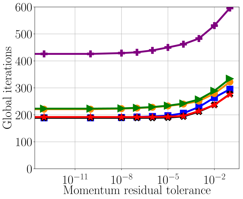
(a) $10^{-11}$ relative residual tolerance.

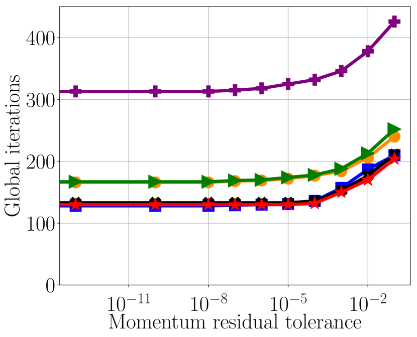
(b) $10^{-8}$ relative residual tolerance.

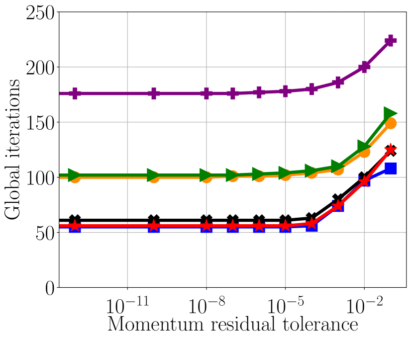
(c) $10^{-5}$ relative residual tolerance.

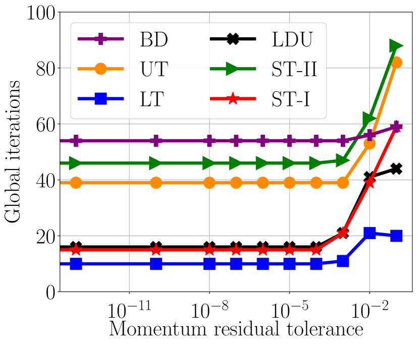
(d) $10^{-3}$ relative residual tolerance.

Figure 2: Number of iterations for the $2\times 2$ block preconditioned system to converge to $10^{-11}$, $10^{-8}$, $10^{-5}$, and $10^{-3}$ relative residual tolerance, as a function of the relative residual tolerance to solve the momentum block. Results are shown for block lower-triangular (LT), block upper-triangular (UT), symmetric lower-then-upper block-triangular (ST-I), symmetric upper-then-lower block-triangular (ST-II), block-diagonal (BD), and approximate block-LDU (LDU) preconditioners.

1. For four different relative-residual tolerances of the $2\times 2$ block system, block-diagonal preconditioning takes very close to twice as many iterations as block-triangular preconditioning. For larger tolerances such as $10^{-3}$, it is approximately twice the average number of iterations of block upper- and block lower-triangular preconditioning, which is consistent with the derivations and constants in Theorem 3.10. Moreover, this relationship holds for almost all tolerances of the momentum block solve, with the exception of considering both large momentum tolerances ($>10^{-3}$) and large global tolerances (see Fig. 2(d)).

2. At no point does a symmetric block-triangular or approximate block-LDU preconditioner offer improved convergence over a block-triangular preconditioner, regardless of momentum or $2\times 2$ system residual tolerance, although the solve times are significantly longer due to the additional applications of the diagonal blocks of the preconditioner. In fact, for a global tolerance of $10^{-3}$ symmetric block-triangular preconditioning is actually less effective than just block triangular.

3. The block lower-triangular preconditioner is more effective than the block-upper-triangular preconditioner. However, they differ in iteration count by roughly the same 30–40 iterations for all four tolerances tested, indicating it is not a difference in convergence rate (which the theory says it should not be), but rather a difference in the leading constants. Interestingly, it cannot be explained by the norm of off-diagonal blocks (which are similar for upper- and lower-triangular preconditioning in this case). We hypothesize it is due to the initial residual, where for $\mathbf{r}^{(0)}=[\mathbf{r}_{1}^{(0)},\mathbf{r}_{2}^{(0)}]$, we have $\|\mathbf{r}_{1}^{(0)}\|=19.14$ and $\|\mathbf{r}_{2}^{(0)}\|=0.0063$. Heuristically, it seems more effective in terms of convergence to solve directly on the block with the large initial residual (in this case the (1,1)-block) and lag the variable with a small initial residual (in this case the (2,2)-block), which would correspond to block-lower triangular preconditioning. However, a better understanding of upper vs. lower block-triangular preconditioning is ongoing work.

A common approach for saddle-point problems that are self-adjoint in a given inner product is to use an SPD preconditioner so that three-term recursion formulae, in particular preconditioned MINRES, can be used. For matrices with saddle-point structure, the Schur complement is often negative definite, so this is achieved by preconditioning $S_{22}$ with some approximation $-\widehat{S}_{22}^{-1}$. Although this is advantageous in terms of being able to use MINRES, convergence can suffer compared with GMRES and an indefinite preconditioner.

Results of this paper indicate a direct correlation between the minimizing polynomial for the $2\times 2$ system and the preconditioned Schur complement. Moreover, convergence on the preconditioned Schur complement should be independent of sign, because Krylov methods minimize over a Krylov space that is invariant to the sign of $M^{-1}$. Together, this indicates that if the (1,1)-block is inverted exactly, convergence of GMRES applied to the $2\times 2$ preconditioned system should be approximately equivalent, regardless of sign of the Schur-complement preconditioner.

Figure 3 demonstrates this property, considering FGMRES iterations on the $2\times 2$ system to relative-residual tolerances of $10^{-11}$ and $10^{-5}$, as a function of momentum relative-residual tolerance. Results are shown for block-diagonal, block lower-triangular, and block-upper-triangular preconditioners, with a natural sign $\widehat{S}_{22}^{-1}$ (solid lines) and swapped sign $-\widehat{S}_{22}^{-1}$ (dotted lines). For accurate solves of the momentum block, we see relatively tight convergence behaviour between $\pm\widehat{S}_{22}^{-1}$. As the momentum solve tolerance is relaxed, convergence of block-triangular preconditioners decay for $-\widehat{S}_{22}^{-1}$. Interestingly, the same phenomenon does not appear to happen for block-diagonal preconditioners, and rather there is a fixed difference in iteration count between $\pm\widehat{S}_{22}^{-1}$. This is likely because a block-diagonal preconditioner does not directly couple the variables of the $2\times 2$ matrix, while the block-triangular preconditioner does. An inexact inverse loses a nice cancellation property of the exact inverse, and the triangular coupling introduces terms along the lines of $I\pm\widehat{S}_{22}^{-1}A_{22}$ (see Eq. 6), which clearly depend on the sign of $\widehat{S}_{22}^{-1}$.

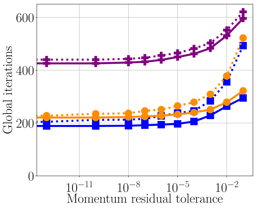
(a) $10^{-11}$ relative residual tolerance.

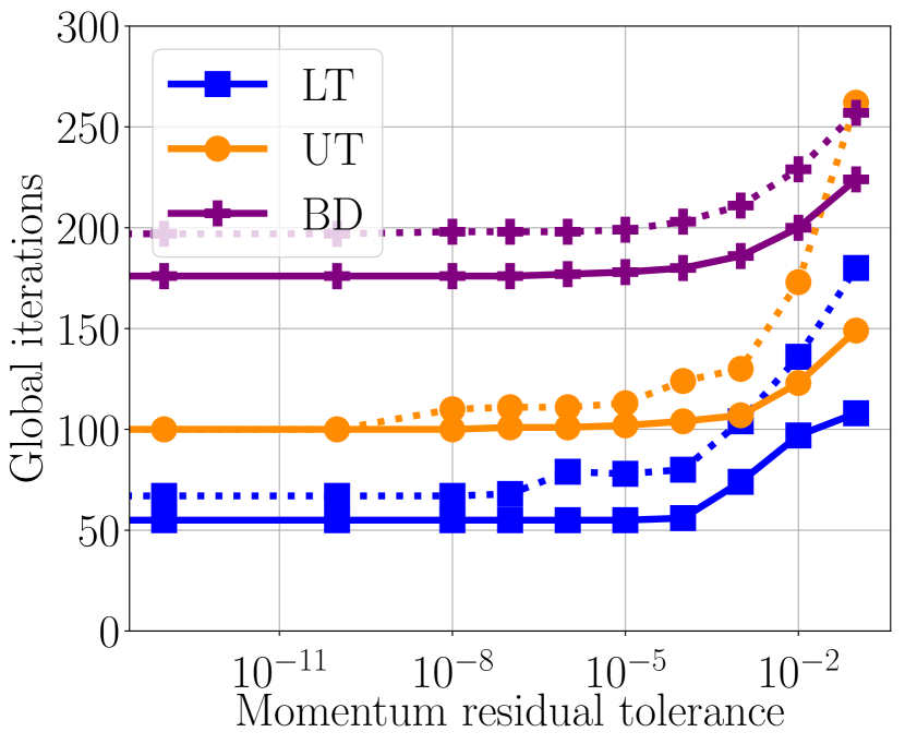
(b) $10^{-5}$ relative residual tolerance.

Figure 3: Number of iterations for the $2\times 2$ block preconditioned system to converge to $10^{-11}$ and $10^{-5}$ relative residual tolerance, as a function of the relative residual tolerance to solve the momentum block. Results are shown for block lower-triangular (LT), block upper-triangular (UT), and block-diagonal (BD) preconditioners, as in Fig. 2 (solid lines) and with the sign swapped on the pressure Schur-complement approximation (dotted lines).

In [14] it is proven that minimal residual methods applied to saddle-point problems with a zero (2,2)-block and preconditioned with a block-diagonal preconditioner observe a staircasing effect, where every alternate iteration stalls. This results in approximately twice as many iterations to convergence as a similar block-triangular preconditioner. Although the proof appeals to specific starting vectors, the effect is demonstrated in practice as well. Theorem 3.10 proved block-diagonal preconditioning is expected to take twice as many iterations as block-triangular preconditioning to reach a given tolerance (within some constant multiplier). Figure 4 looks at the GMRES convergence factor as a function of iteration for block-diagonal preconditioning and block lower-triangular preconditioning, with $\pm\widehat{S}_{22}^{-1}$. Interestingly, with $-\widehat{S}_{22}^{-1}$ (see Fig. 4(b)), the staircasing effect is clear, where every alternate iteration makes little to no reduction in residual. Although convergence has some sawtooth character for block-diagonal with $\widehat{S}_{22}^{-1}$ as well, it is much weaker, and the staircasing effect is not truly observed. It is possible this explains the slightly better convergence obtained with $\widehat{S}_{22}^{-1}$ in Fig. 3(b), regardless of momentum relative-residual tolerance.

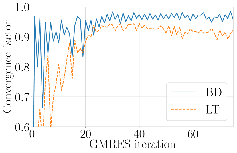
(a) Preconditioning using $\widehat{S}_{22}^{-1}$.

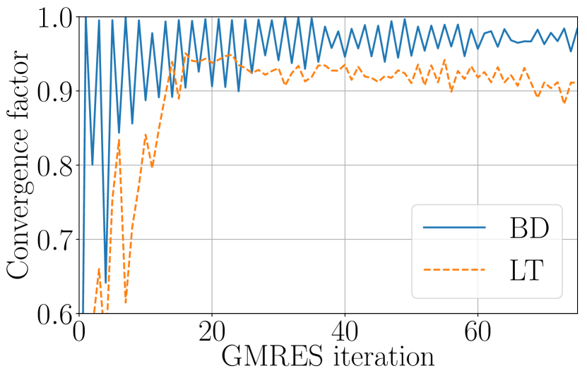
(b) Preconditioning using $-\widehat{S}_{22}^{-1}$.

Figure 4: Convergence factor as a function of FGMRES iteration for block-diagonal (BD) and block lower-triangular (LT) preconditioning. Figure 4(a) uses the natural sign on $\widehat{S}_{22}^{-1}$, while Fig. 4(b) adds a negative to $\widehat{S}_{22}^{-1}$.

5 Conclusions

This paper analyzes the relationship between Krylov methods with $2\times 2$ block preconditioners and the underlying preconditioned Schur complement. Under the assumption that one of the diagonal blocks is inverted exactly, we prove a direct relationship between the minimizing Krylov polynomial of a given degree for the two systems, thereby proving their equivalence and the fact that an effective Schur complement preconditioner is a necessary and sufficient condition for an effective $2\times 2$ block preconditioner. Theoretical results give further insight into choice of block preconditioner, including that (i) symmetric block-triangular and approximate block-LDU preconditioners offer a minimal reduction in iteration count over block-triangular preconditioners, at the expense of additional computational cost, and (ii) block-diagonal preconditioners take about twice as many iterations to reach a given residual tolerance as block-triangular preconditioners.

Numerical results on an HDG discretization of the steady linearized Navier–Stokes equations confirm the theoretical contributions, and show that the practical implications extend to the case of a Schur-complement approximation coupled with an inexact inverse of the other diagonal block. Although not shown here, it is worth pointing out we have observed similar results with inexact block preconditioners in other applications. For HDG discretizations of symmetric Stokes and Darcy problems, if the pressure Schur complement is approximated by a spectrally equivalent operator, applying two to four multigrid cycles to the momentum block yields comparable convergence on the larger $2\times 2$ system as applying a direct solve on the momentum block. Classical source iteration and DSA preconditioning for S_N discretizations of neutron transport can also be posed as a $2\times 2$ block preconditioning [38]. There we have also observed that when applying AMG iterations to the (1,1)-block and Schur complement approximation, only 2-3 digits of residual reduction yields convergence on the larger $2\times 2$ system in a similar number of iterations as applying direct solves to each block. In each of these cases, convergence of minimal residual methods applied to the $2\times 2$ system is defined by the preconditioning of the Schur complement.

Appendix A Proof of Theorem 3.4

Proof A.1 (Proof of Theorem 3.4).

Here we prove the case of $k=2$. An analogous derivation appealing to Eq. 10 yields equivalent results for $k=1$.

Recall that CG forms a minimizing consistent polynomial of $M_{22}^{-1}A$ in the $A$-norm. Let $\varphi^{(d)}$ be the minimizing polynomial of degree $d$ in $M_{22}^{-1}A$ for error vector $\mathbf{e}$ in the $A$-norm. Then, expressing $A$ in a block LDU sense to simplify the term $A\varphi^{(d+1)}(M_{22}^{-1}A)$, we immediately obtain a lower bound:

$$\|\varphi^{(d)}(M_{22}^{-1}A)\mathbf{e}\|_{A}^{2} =\langle A\varphi^{(d)}(M_{22}^{-1}A)\mathbf{e},\varphi^{(d)}(M_{22}^{-1}A)\mathbf{e}\rangle$$

$$=\left\langle\begin{bmatrix}A_{11}&\mathbf{0}\\ \mathbf{0}&S_{22}\end{bmatrix}\begin{bmatrix}\varphi^{(d)}(I)(\mathbf{e}_{1}+A_{11}^{-1}A_{12}\mathbf{e}_{2})\\ \varphi^{(d)}(\widehat{S}_{22}^{-1}S_{22})\mathbf{e}_{2}\end{bmatrix},\begin{bmatrix}\varphi^{(d)}(I)(\mathbf{e}_{1}+A_{11}^{-1}A_{12}\mathbf{e}_{2})\\ \varphi^{(d)}(\widehat{S}_{22}^{-1}S_{22})\mathbf{e}_{2}t\end{bmatrix}\begin{bmatrix}\mathbf{e}_{1}\\ \mathbf{e}_{2}\end{bmatrix}\right\rangle$$

$$\geq\langle S_{22}\varphi^{(d)}(\widehat{S}_{22}^{-1}S_{22})\mathbf{e}_{2},\varphi^{(d)}(\widehat{S}_{22}^{-1}S_{22})\mathbf{e}_{2}\rangle$$

$$=\|\varphi^{(d)}(\widehat{S}_{22}^{-1}S_{22})\mathbf{e}_{2}\|_{S_{22}}^{2}$$

$$=\|\varphi_{22}^{(d)}(\widehat{S}_{22}^{-1}S_{22})\mathbf{e}_{2}\|_{S_{22}}^{2},$$

where $\varphi_{22}^{(d)}$ is the minimizing polynomial of degree $d$ in $\widehat{S}_{22}^{-1}S_{22}$ for error vector $\mathbf{e}_{2}$. A lower bound on the minimizing polynomial of degree $d$ in norm follows immediately by noting that

$$\|\varphi^{(d)}(M_{22}^{-1}A)\|_{A} =\sup_{\mathbf{e}\neq\mathbf{0}}\frac{\|\varphi^{(d)}(M_{22}^{-1}A)\mathbf{e}\|_{A}}{\|\mathbf{e}\|_{A}}\geq\sup_{\begin{subarray}{c}\mathbf{e}_{2}\neq\mathbf{0},\\ \mathbf{e}_{1}=-A_{11}^{-1}A_{12}\end{subarray}}\frac{\|\varphi^{(d)}(M_{22}^{-1}A)\mathbf{e}\|_{A}}{\|\mathbf{e}\|_{A}}$$

$$\hskip 12.91663pt=\|\varphi^{(d)}(\widehat{S}_{22}^{-1}S_{22})\|_{S_{22}}\geq\|\varphi_{22}^{(d)}(\widehat{S}_{22}^{-1}S_{22})\|_{S_{22}}.$$

For an upper bound, let $\varphi_{22}^{(d)}$ be the minimizing polynomial of degree $d$ in $\widehat{S}_{22}^{-1}S_{22}$ for error vector $\mathbf{e}_{2}$ in the $S_{22}$-norm. Define the degree $d+1$ polynomial $q(t)\mathrel{\mathop{\mathchar 58\relax}}=(1-t)\varphi^{(d)}_{22}(t)$, and let $\varphi^{(d+1)}$ be the minimizing polynomial of degree $d+1$ in $M_{22}^{-1}A$ for error vector $\mathbf{e}$ in the $A$-norm. Then

$$\|\varphi^{(d+1)}(M_{22}^{-1}A)\mathbf{e}\|_{A}^{2} \leq\|q(M_{22}^{-1}A)\mathbf{e}\|_{A}^{2}$$

$$=\left\langle\begin{bmatrix}A_{11}&\mathbf{0}\\ \mathbf{0}&S_{22}\end{bmatrix}\begin{bmatrix}\mathbf{0}&\mathbf{0}\\ \mathbf{0}&q(\widehat{S}_{22}^{-1}S_{22})\end{bmatrix}\begin{bmatrix}\mathbf{e}_{1}\\ \mathbf{e}_{2}\end{bmatrix},\begin{bmatrix}\mathbf{0}&\mathbf{0}\\ \mathbf{0}&q(\widehat{S}_{22}^{-1}S_{22})\end{bmatrix}\begin{bmatrix}\mathbf{e}_{1}\\ \mathbf{e}_{2}\end{bmatrix}\right\rangle$$

$$=\langle S_{22}q(\widehat{S}_{22}^{-1}S_{22})\mathbf{e}_{2},q(\widehat{S}_{22}^{-1}S_{22})\mathbf{e}_{2}\rangle$$

$$=\|(I-\widehat{S}_{22}^{-1}S_{22})\varphi_{22}^{(d)}(\widehat{S}_{22}^{-1}S_{22})\mathbf{e}_{2}\|_{S_{22}}^{2}.$$

For a bound in norm, note that for a fixed $\mathbf{e}_{2}$, $\|\mathbf{e}\|_{A}^{2}$ is a quadratic function in $\mathbf{e}_{1}$, with minimum obtained at $\mathbf{e}_{1}\mathrel{\mathop{\mathchar 58\relax}}=-A_{11}^{-1}A_{12}$. Then,

$$\|\varphi^{(d+1)}(M_{22}^{-1}A)\|_{A}^{2} =\sup_{\mathbf{e}\neq\mathbf{0}}\frac{\|\varphi^{(d+1)}(M_{22}^{-1}A)\mathbf{e}\|_{A}^{2}}{\|\mathbf{e}\|_{A}^{2}}\leq\sup_{\mathbf{e}\neq\mathbf{0}}\frac{\|q(M_{22}^{-1}A)\mathbf{e}\|_{A}^{2}}{\|\mathbf{e}\|_{A}^{2}}$$

$$=\sup_{\mathbf{e}_{2}}\frac{\|(I-\widehat{S}_{22}^{-1}S_{22})\varphi_{22}^{(d)}(\widehat{S}_{22}^{-1}S_{22})\mathbf{e}_{2}\|_{S_{22}}^{2}}{\inf_{\mathbf{e}_{1}}\|\mathbf{e}\|_{A}^{2}}=\sup_{\mathbf{e}_{2}}\frac{\|(I-\widehat{S}_{22}^{-1}S_{22})\varphi_{22}^{(d)}(\widehat{S}_{22}^{-1}S_{22})\mathbf{e}_{2}\|_{S_{22}}^{2}}{\|\mathbf{e}_{2}\|_{S_{22}}^{2}}$$

$$=\|(I-\widehat{S}_{22}^{-1}S_{22})\varphi_{22}^{(d)}(\widehat{S}_{22}^{-1}S_{22})\|_{S_{22}}^{2}.$$

References

• [1] S. F. Ashby, T. A. Manteuffel, and P. E. Saylor, A taxonomy for conjugate gradient methods, SIAM Journal on Numerical Analysis, 27 (1990), pp. 1542–1568.
• [2] O. Axelsson and M. Neytcheva, Eigenvalue estimates for preconditioned saddle point matrices, Numerical Linear Algebra with Applications, 13 (2006), pp. 339–360, https://doi.org/10.1002/nla.469.
• [3] Z. Z. Bai, Structured preconditioners for nonsingular matrices of block two-by-two structures, Mathematics of Computation, 75 (2006), pp. 791–815.
• [4] Z. Z. Bai and M. K. Ng, On inexact preconditioners for nonsymmetric matrices, SIAM Journal on Scientific Computing, 26 (2005), pp. 1710–1724.
• [5] S. Balay, S. Abhyankar, M. F. Adams, J. Brown, P. Brune, K. Buschelman, L. Dalcin, V. Eijkhout, W. D. Gropp, D. Kaushik, M. G. Knepley, L. C. McInnes, K. Rupp, B. F. Smith, S. Zampini, H. Zhang, and H. Zhang, PETSc users manual, Tech. Report ANL-95/11 - Revision 3.7, Argonne National Laboratory, 2016, http://www.mcs.anl.gov/petsc.
• [6] M. Benzi and M. A. Olshanskii, Field-of-values convergence analysis of augmented Lagrangian preconditioners for the linearized Navier–Stokes problem, SIAM Journal on Numerical Analysis, 49 (2011), pp. 770–788.
• [7] M. Benzi, M. A. Olshanskii, and Z. Wang, Modified augmented Lagrangian preconditioners for the incompressible Navier–Stokes equations, International Journal for Numerical Methods in Fluids, 66 (2011), pp. 486–508.
• [8] F. Brezzi, L. D. Marini, and E. Süli, Discontinuous Galerkin methods for first-order hyperbolic problems, Mathematical models and methods in applied sciences, 14 (2004), pp. 1893–1903.
• [9] E. C. Cyr, J. N. Shadid, and R. S. Tuminaro, Stabilization and scalable block preconditioning for the Navier–Stokes equations, Journal of Computational Physics, 231 (2012), pp. 345–363.
• [10] V. A. Dobrev, T. V. Kolev, et al., MFEM: Modular finite element methods. http://mfem.org, 2018.
• [11] H. S. Dollar, N. I. Gould, M. Stoll, and A. J. Wathen, Preconditioning saddle-point systems with applications in optimization, SIAM Journal on Scientific Computing, 32 (2010), pp. 249–270.
• [12] H. Elman and D. Silvester, Fast nonsymmetric iterations and preconditioning for Navier–Stokes equations, SIAM Journal on Scientific Computing, 17 (1996), pp. 33–46.
• [13] R. D. Falgout and U. M. Yang, hypre: A library of high performance preconditioners, European Conference on Parallel Processing, 2331 LNCS (2002), pp. 632–641.
• [14] B. Fischer, A. Ramage, D. J. Silvester, and A. J. Wathen, Minimum residual methods for augmented systems, BIT, 38 (1998), pp. 527–543.
• [15] A. Greenbaum, V. Pták, and Z. Strakoš, Any nonincreasing convergence curve is possible for GMRES, SIAM Journal on Matrix Analysis and Applications, 17 (1996), pp. 465–469.
• [16] I. C. F. Ipsen, A note on preconditioning nonsymmetric matrices, SIAM Journal on Scientific Computing, 23 (2001), pp. 1050–1051.
• [17] A. Klawonn, Block-triangular preconditioners for saddle point problems with a penalty term, SIAM Journal on Scientific Computing, 19 (1998), pp. 172–184.
• [18] A. Klawonn and G. Starke, Block triangular preconditioners for nonsymmetric saddle point problems: field-of-values analysis, Numerische Mathematik, 81 (1999), pp. 577–594.
• [19] P. Krzyzanowski, On block preconditioners for nonsymmetric saddle point problems, SIAM Journal on Scientific Computing, 23 (2001), pp. 157–169.
• [20] D. Loghin and A. Wathen, Analysis of preconditioners for saddle-point problems, SIAM Journal on Scientific Computing, 25 (2004), pp. 2029–2049.
• [21] Y. Ma, K. Hu, X. Hu, and J. Xu, Robust preconditioners for incompressible mhd models, Journal of Computational Physics, 316 (2016), pp. 721–746.
• [22] T. A. Manteuffel, The Tchebychev iteration for nonsymmetric linear systems, Numerische Mathematik, (1977), pp. 307–327.
• [23] T. A. Manteuffel, S. Munzenmaier, J. Ruge, and B. S. Southworth, Nonsymmetric reduction-based algebraic multigrid, SIAM J. Sci. Comput., 41 (2019), pp. S242–S268.
• [24] T. A. Manteuffel, J. Ruge, and B. S. Southworth, Nonsymmetric algebraic multigrid based on local approximate ideal restriction ($\ell$AIR), SIAM J. Sci. Comput., 40 (2018), pp. A4105–A4130.
• [25] E. McDonald, S. Hon, J. Pestana, and A. J. Wathen, Preconditioning for nonsymmetry and time-dependence, in Domain decomposition methods in science and engineering XXIII, Springer, Cham, 2017, pp. 81–91.
• [26] M. F. Murphy, G. H. Golub, and A. Wathen, A note on preconditioning for indefinite linear systems, SIAM Journal on Scientific Computing, 21 (2000), pp. 1969–1972.
• [27] Y. Notay, A new analysis of block preconditioners for saddle point problems, SIAM Journal on Matrix Analysis and Applications, 35 (2014), pp. 143–173.
• [28] J. W. Pearson and A. J. Wathen, A new approximation of the Schur complement in preconditioners for PDE-constrained optimization, Numerical Linear Algebra with Applications, 19 (2011), pp. 816–829.
• [29] J. Pestana, On the eigenvalues and eigenvectors of block triangular preconditioned block matrices, SIAM Journal on Matrix Analysis and Applications, 35 (2014), pp. 517–525.
• [30] J. Pestana and A. J. Wathen, Combination preconditioning of saddle point systems for positive definiteness, Numerical Linear Algebra with Applications, 20 (2012), pp. 785–808.
• [31] T. Rees and M. Stoll, Block-triangular preconditioners for PDE-constrained optimization, Numerical Linear Algebra with Applications, 17 (2010), pp. 977–996.
• [32] S. Rhebergen and G. N. Wells, A hybridizable discontinuous Galerkin method for the Navier–Stokes equations with pointwise divergence-free velocity field, J. Sci. Comput., 76 (2018), pp. 1484–1501.
• [33] Y. Saad, A flexible inner-outer preconditioned gmres algorithm, SIAM Journal on Scientific Computing, 14 (1993), pp. 461–469.
• [34] J. Schöberl and W. Zulehner, Symmetric indefinite preconditioners for saddle point problems with applications to PDE-constrained optimization problems, SIAM Journal on Matrix Analysis and Applications, 29 (2007), pp. 752–773.
• [35] C. Siefert and E. de Sturler, Preconditioners for generalized saddle-point problems, SIAM Journal on Numerical Analysis, 44 (2006), pp. 1275–1296.
• [36] D. Silvester and A. Wathen, Fast Iterative Solution of Stabilised Stokes Systems Part II: Using General Block Preconditioners, SIAM Journal on Numerical Analysis, 31 (1994), pp. 1352–1367, https://doi.org/10.1137/0731070.
• [37] A. A. Sivas, B. S. Southworth, and S. Rhebergen, A Re-robust preconditioner for an HDG discretization of Navier–Stokes, (in preparation).
• [38] B. S. Southworth, M. Holec, and T. S. Haut, Diffusion synthetic acceleration for heterogeneous domains, compatible with voids, arXiv preprint arXiv:2001.09196, (2020).
• [39] B. S. Southworth and S. S. Olivier, A note on $2\times 2$ block-diagonal preconditioning, arXiv preprint arxiv:2001.00711, (2020).
• [40] J. D. Tebbens and G. Meurant, Prescribing the behavior of early terminating GMRES and Arnoldi iterations, Numerical Algorithms, 65 (2013), pp. 69–90.
• [41] A. Wathen, Preconditioning and convergence in the right norm, International Journal of Computer Mathematics, 84 (2007), pp. 1199–1209.
• [42] J. A. White and R. I. Borja, Block-preconditioned Newton–Krylov solvers for fully coupled flow and geomechanics, Computational Geosciences, 15 (2011), p. 647.