Entanglement and classical fluctuations at finite-temperature critical points

Abstract

We investigate several entanglement-related quantities at finite-temperature criticality in the three-dimensional quantum spherical model, both as a function of temperature $T$ and of the quantum parameter $g$, which measures the strength of quantum fluctuations. While the von Neumann and the Rényi entropies exhibit the volume-law for any $g$ and $T$, the mutual information obeys an area law. The prefactors of the volume-law and of the area-law are regular across the transition, reflecting that universal singular terms vanish at the transition. This implies that the mutual information is dominated by nonuniversal contributions. This hampers its use as a witness of criticality, at least in the spherical model. We also study the logarithmic negativity. For any value of $g,T$, the negativity exhibits an area-law. The negativity vanishes deep in the paramagnetic phase, it is larger at small temperature, and it decreases upon increasing the temperature. For any $g$, it exhibits the so-called sudden death, i.e., it is exactly zero for large enough $T$. The vanishing of the negativity defines a “death line”, which we characterise analytically at small $g$. Importantly, for any finite $T$ the area-law prefactor is regular across the transition, whereas it develops a cusp-like singularity in the limit $T\to 0$. Finally, we consider the single-particle entanglement and negativity spectra. The vast majority of the levels are regular across the transition. Only the larger ones exhibit singularities. These are related to the presence of a zero mode, which reflects the symmetry breaking. This implies the presence of sub-leading singular terms in the entanglement entropies. Interestingly, since the larger levels do not contribute to the negativity, sub-leading singular corrections are expected to be suppressed for the negativity.

I Introduction

Understanding the interplay between entanglement and classical fluctuations in quantum many-body systems is a challenging task. Several entanglement-related quantities have been investigated area ; amico-2008 ; calabrese-2009 ; laflorencie-2016 . Arguably, the most popular ones are the Rényi entropies and the von Neumann entropy. Given a partition of the system in subsystems $A$ and its complement $B\equiv\bar{A}$ (see Fig. 1 (a) for a three-dimensional setup), the Rényi entropies $S_{n}$ are defined as

$$S_{n}\equiv\frac{1}{1-n}\ln\textrm{Tr}\rho_{A}^{n},$$ (1)

with $\rho_{A}$ the reduced density matrix of part $A$. In the limit $n\to 1$ one obtains the so-called von Neumann entropy $S=-\textrm{Tr}\rho_{A}\ln\rho_{A}$. If the total system $A\cup\bar{A}$ is in a pure state, $S_{n}$ are good measures of the entanglement between $A$ and the rest. At zero temperature the famous area-law behaviour $S_{n}\propto L^{d-1}$ holds true, with $L$ being the linear size of the system, and $d$ the dimensionality. Logarithmic corrections are present for gapless fermionic systems wolf-2006 ; gioev-2006 ; cmv-11d . This is strikingly different at finite temperature, where $S_{n}$ cannot distinguish genuine quantum correlations from thermal ones. At finite temperature the volume-law behaviour $S_{n}\propto L^{d}$ holds, reflecting, for instance, the transformation between entanglement and standard thermodynamic entropy. In this situation, the mutual information $I_{n,A:\bar{A}}$ (see section II for its definition) can be used to measure the total correlation, i.e., both classical and quantum, between $A$ and $\bar{A}$. The mutual information exhibits the area-law behaviour $I_{n}\propto L^{d-1}$. Still, $I_{n}$ is not a proper measure of the mutual entanglement between $A$ and $\bar{A}$. This reflects $A\cup\bar{A}$ being in a mixed state. The so-called logarithmic negativity lee-2000 ; vidal-2002 ; plenio-2005 is the most popular entanglement measure for mixed states. For systems described by Conformal Field Theory, its behaviour has been fully characterized, both at zero temperature calabrese-2012 , and at finite temperature calabrese-2015 . Similar to the mutual information, for any temperature the negativity exhibits the area-law scaling, which has been checked in several systems dct-16 ; eisler-2016 ; shapourian-2018 ; tarun-1 ; tarun-2 .

An important question, which is key in this paper, is how quantum and classical fluctuations are intertwined at a finite temperature critical point. An important remark is that typical local one dimensional models do not exhibit finite-temperature or mid-spectrum criticality, with the notable exception of models that exhibit the many-body localisation transition nandi . It has been argued that entanglement-related quantities can be used to detect this transition khemani-17 ; kjall-2014 ; chandran-2015 ; laflorencie-2016 , although no conclusion has been reached, due the severe finite-size effects. On the other hand, although standard finite-temperature phase transitions are possible in higher dimensions, the interplay between classical and quantum fluctuations at finite-temperature criticality has been scarcely studied, despite the growing interest hauke-2016 ; gabrielli-2018 ; frerot-2019 . Much efforts focused on the behaviour of the mutual information. For instance, it has been suggested singh-2011 ; melko-2010 ; kallin-2013 ; inglis-2013 ; srilu-2018 ; singh-2012 that the mutual information exhibits a crossing for different sizes at a finite-temperature critical point, similar to more traditional tools in critical phenomena, such as the Binder cumulant vicari .

Importantly, there is growing interest to understand the behaviour of the logarithmic negativity at finite-temperature criticality. An important question is whether the logarithmic negativity exhibits signatures of criticality. Since finite-temperature phase transitions are driven by classical fluctuations, and the negativity is only sensitive to true quantum correlations, one should expect the negativity to be smooth across a finite-temperature critical point. Surprisingly, it has been observed that the negativity can exhibit “weak” singularities, such as cusp-like features, at the critical point tarun-1 ; tarun-2 ; lu-2018 . On the other hand, similar singularities have been also observed in the area-law prefactor of the Rényi entropies at quantum phase transitions helmes-2014 ; frerot-2016 .

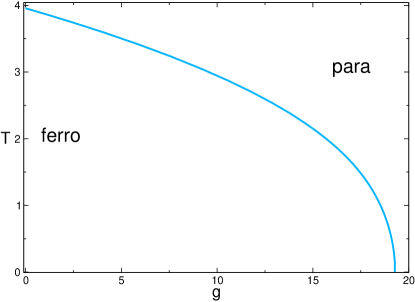
In this paper we investigate the behaviour of several entanglement-related observables at finite-temperature criticality. Specifically, we consider the Rényi entropies (and the von Neumann entropy), the mutual information, and the logarithmic negativity. We also discuss the so-called single-particle entanglement spectrum and the negativity spectrum. To be specific, here we focus on the paradigmatic quantum spherical model (QSM) in three dimensions. Spherical models have a venerable history, as they served as test ground for the theory of critical phenomena and the theory of finite-size scaling joyce-1972 ; brankov . The phase diagram of the model (see Fig. 2) is spanned by the temperature $T$ and the so-called quantum coupling $g$. The latter measures the strength of the quantum fluctuations. In three dimensions, the model exhibits a line of finite-temperature second-order phase transitions between a paramagnetic phase and a ferromagnetically ordered phase. The universality class of the transition has been characterised analytically, since the model is exactly solvable, and it is that of the $N$-vector model vicari in the limit $N\to\infty$ limit zinn-1998 . Surprisingly, the entanglement properties of spherical models have not been explored much.

First, we verify that the entanglement entropy and the Rényi entropies exhibit the expected volume-law in the whole phase diagram. In the thermodynamic limit, the prefactor of the volume-law and its first derivative with respect to the model parameters and the temperature are continuous across the transition. We refer to this behaviour as regular. Conversely, we refer to non-analytic behaviour as singular. This means that, although the entanglement entropies contain singular contributions, these vanish at the transition as $|g-g_{c}|^{\kappa}$ (or as $|T-T_{c}|^{\kappa}$) with $\kappa>1$, and $T_{c}$ and $g_{c}$ marking the critical point. The mutual information between two regions exhibits the expected area-law behaviour for any value of $g$ and $T$. Moreover, although the prefactor of the area law contains both regular and singular contributions at criticality, again, we observe regular behaviour across the transition, suggesting that the singular terms vanish. Interestingly, for finite-size systems we observe that the mutual information does not exhibit a universal crossing at the transition. This reflects that the singular terms, which contain universal information, are vanishing at the critical point, and the mutual information is dominated by non-universal contributions. We find a similar behaviour for the logarithmic negativity. The negativity exhibits the expected area-law in the whole phase diagram. The area-law prefactor has a maximum at the phase transition. In the paramagnetic phase the negativity vanishes as $1/g$ in the limit $g\to\infty$. In the ordered phase it depends mildly on the system parameters for low enough temperature and large enough values of $g$. For any fixed value of $g$, the negativity exhibits a “sudden death” upon increasing the temperature. Specifically, there is a negativity “death line”, above which the negativity is exactly zero. Interestingly, in the limit $g\to 0$, i.e., when the model becomes classical, the death line exhibits the behaviour $\propto g^{1/2}$. Importantly, at finite temperature the prefactor of the area-law is regular across the para-ferro transition, whereas it develops a cusp-like feature upon lowering the temperature.

Finally, we discuss the single-particle entanglement spectrum laflorencie-2016 and the negativity spectrum ruggiero-2016a . For two nearest-neighbour sites in an infinite system, the spectrum contains only two levels. One of the levels is regular across the transition, whereas the other exhibits a cusp singularity. This is different for the negativity between two extended subsystems. Specifically, we observe that the majority of the single-particle entanglement spectrum levels show regular behaviour at the transition. Only the larger levels exhibit a cusp-like behaviour. Interestingly, the corresponding eigenvectors show a flat-in-space structure, suggesting that the singular levels originate from the zero mode, which is associated with the symmetry breaking. As it is well known, this zero mode leads to sub-leading logarithmic terms met-grov ; alba-2012 in the entropies. This also means that, although the prefactor of the volume law behaviour of the entropies is regular across the transition, the sub-leading corrections exhibit signatures of the criticality. We observe a similar structure for the negativity spectrum. However, since the larger negativity spectrum levels do not contribute to the logarithmic negativity, this suggests that the sub-leading singular terms are suppressed.

The manuscript is organised as follows. In section II we introduce the entanglement-related quantities that we consider in the paper. In section III we review the quantum spherical model. Specifically, in section III.1 we provide the results for the two-point correlation functions, discussing their behaviour in the paramagnetic phase, and in the ordered phase (in section III.2 and section III.3, respectively). In section IV we address the critical behaviour of the model. Criticality is encoded in the so-called spherical parameter that we discuss in section IV.1. In section IV.2 we focus on the correlators near the para-ferro transition. In order to compare entanglement-related quantities with standard thermodynamic ones, in section IV.3 and section IV.4 we discuss the singular behaviour of the free energy, and of the universal ratio $R_{\xi}$. In section V we focus on the interplay between entanglement and finite-temperature criticality. In section V.2 and section V.3 we study the entanglement entropy, and the mutual information. In section VI we present our results for the logarithmic negativity. In section VI.1 we focus on the negativity between two sites embedded in an infinite system, whereas in section VI.2 we discuss the negativity between two extended regions. In section VII we investigate the single-particle entanglement spectrum and the negativity spectrum. Finally, we conclude in section VIII.

Figure 1: Geometry used in this work. The quantum spherical model lives on a $3D$ cubic lattice of linear size $L$ (see (a)). Periodic boundary conditions are used in all directions. In (b) the total system is divided into two parts as $A\cup B$, and $B$ is traced over. Here $\ell_{x}\times\ell_{y}\times\ell_{z}$ is the volume of $A$. In (c) subsystem $A$ is further divided as $A=A_{1}\cup A_{2}$. Here we consider the entanglement between the two adjacent cubic blocks $A_{1}$ and $A_{2}$. We consider both the case of finite $B$, as well as the limit of $B$ infinite.

II Entanglement entropies, mutual information & logarithmic negativity: Definitions

In this section we introduce the definitions of the entanglement and Rényi entropies, the mutual information, and the so-called logarithmic negativity. Here, we always consider a system on a three-dimensional cubic lattice of linear size $L$ (see Fig. 1 (a)), prepared in a thermal state at temperature $T\equiv 1/\beta$.

In order to define the entanglement entropy (von Neumann entropy) and the Rényi entropies, we consider a bipartition of the system into two parts $A$ and $B$ (see Fig. 1 (b)). From the reduced density matrix for $A$, $\rho_{A}\equiv\textrm{Tr}_{B}\rho$, with $\rho$ being the density matrix of the full system, we define the Rényi entropies $S_{n,A}$ as area ; amico-2008 ; calabrese-2009 ; laflorencie-2016

$$S_{n,A}=\frac{1}{1-n}\textrm{Tr}\rho_{A}^{n},\quad\textrm{with}\,n\in\mathbb{R}.$$ (2)

In the limit $n\to 1$ one obtains the von Neumann entropy as

$$S_{\mathrm{vN}}=-\textrm{Tr}\rho_{A}\ln\rho_{A}.$$ (3)

Both, the von Neumann and the Rényi entropies, are good entanglement measures for pure systems, for instance bipartite systems at zero temperature. This is not the case anymore if $A\cup\bar{A}$, with $\bar{A}$ the complement of $A$, is in a mixed state, for instance a thermal one. In a thermal state, $S_{n,A}$ exhibits a volume-law behaviour $S_{n,A}\propto L^{d}$. For $S_{\mathrm{vN}}$, the prefactor of the volume-law is the same as that of the thermal entropy, i.e., the von Neumann entanglement entropy becomes the thermodynamic entropy at finite temperature dls-13 ; spr-12 ; kaufman-2016 .

The mutual information between two subsystems is defined for the typical geometry depicted in Fig. 1 (c). The subsystem $A$ is divided into two complementary parts viz $A_{1}\cup A_{2}=A$, with $\bar{A}$ in general not empty. The mutual information $I_{n,A_{1}:A_{2}}$ is defined as

$$I_{n,A_{1}:A_{2}}=S_{n,A_{1}}+S_{n,A_{2}}-S_{n,A_{1}\cup A_{2}}.$$ (4)

Here $S_{n,X}$ is the Rényi entropy of subsystem $X$. It is important to note that the mutual information is only a measure of the total correlation shared between the two subsystems, and not of the shared entanglement. This is because $I_{n,A_{1}:A_{2}}$ is sensitive to both, quantum and classical correlations, which is reflected in the fact that $A$ is in a mixed state. Importantly, this is also the case at $T=0$ if $A_{1}\cup A_{2}$ is not the full system, i.e., if $A_{1}$ and $A_{2}$ are not complementary intervals. In this case the classical correlation originates from the trace over the environment, i.e., $\bar{A}$ in (4). It can be shown, however, that the mutual information provides a bound to the mutual entanglement vidal-2002 .

Both the entanglement entropy and the mutual information have been studied intensely as possible witnesses of critical behaviour in several systems (see Ref. laflorencie-2016, for a review), both at finite-temperature phase transitions wilms-2012 ; singh-2011 ; melko-2010 ; inglis-2013 ; jm-2014 ; mandal-2016 ; srilu-2018 , or at $T=0$ phase transitions metlitski-2009 ; singh-2012 ; kallin-2013 ; helmes-2014 ; frerot-2016 . Specifically, in Ref. melko-2010, (see also singh-2011, ) it has been shown that the mutual information densities $I_{n,A_{1}:A_{2}}/L^{d-1}$ exhibit a universal crossing at $T=T_{c}$ and $T=nT_{c}$. On the other hand, at zero temperature, it has been shown that the area-law coefficient of the entanglement entropy displays a cusp-like singularity across a second order phase transition (see for instance Ref. helmes-2014, ).

Here we also consider the so-called logarithmic negativity peres-1996 ; zycz-1998 ; zycz-1999 ; lee-2000 ; vidal-2002 ; plenio-2005 . Unlike the mutual information, the negativity is a good entanglement measure for mixed states. The negativity allows, for instance, to quantify the entanglement in a bipartite system at finite temperature (see Fig. 1 (b)), or the entanglement between two non-complementary subsystems (as in Fig. 1 (c)) at zero temperature. The negativity is defined from the so-called partial transpose. Given the partition of $A$ as $A=A_{1}\cup A_{2}$ (see Fig. 1 (c)), the matrix elements of the partial transpose $\rho_{A}^{T_{2}}$ with respect to the degrees of freedom of $A_{2}$ are defined as

$$\langle\varphi_{1}\varphi_{2}|\rho_{A}^{T_{2}}|\varphi_{1}^{\prime}\varphi_{2}^{\prime}\rangle=\langle\varphi_{1}\varphi_{2}^{\prime}|\rho_{A}|\varphi_{1}^{\prime}\varphi_{2}\rangle.$$ (5)

Here $\{\varphi_{1}\}$ and $\{\varphi_{2}\}$ are two orthonormal bases for $A_{1}$ and $A_{2}$, respectively. Interestingly, the eigenvalues $\zeta_{i}$ of $\rho_{A}^{T_{2}}$ can be both positive and negative. This is in contrast with the eigenvalues of $\rho_{A}$, which can be only positive. The logarithmic negativity ${\cal E}_{A_{1}:A_{2}}$ is defined as

$${\cal E}_{A_{1}:A_{2}}=\ln\textrm{Tr}|\rho_{A}^{T_{2}}|.$$ (6)

Recently, the negativity has become a useful tool to characterise universal aspects of quantum many-body systems hannu-2008 ; mrpr-09 ; hannu-2010 ; calabrese-2012 ; cct-neg-long ; calabrese-2013 ; calabrese-2015 ; kpp-14 ; ruggiero-2016 ; rr-15 ; fournier-2015 ; bc-16 ; lee-2013 ; castelnovo-2013 ; hart-2018 ; java-2018 ; bayat-2012 ; bayat-2014 ; abab-16 ; wen-2016 ; wen-2016a ; ruggiero-2016a ; glen ; alba-e ; gs-18 ; dct-15 ; gbbs-17 ; csg-18 ; sherman-2016 ; lu-2018 ; hassan-2019 ; xhek-2019 , also because it can be computed with Matrix Product States (MPS) methods hannu-2008 ; calabrese-2013 ; ruggiero-2016 . The negativity (6) can be obtained for free-bosonic models in arbitrary dimension by correlation matrix techniques audenaert-2002 ; eisler-2016 ; dct-16 . This is not possible for free-fermion models eisler-2014a ; coser-2015 ; ctc-16 ; chang-2016 ; hw-16 ; shapourian-2016 ; ssr-16 ; eez-16 . An alternative entanglement measure, which is effectively calculable using free-fermion techniques, has been introduced  shapourian-2016 ; ssr-16 ; shiozaki-2017 ; shiozaki-2018 ; shapourian-2018 ; shapourian-2018a , and it is also an upper bound for the negativity  eez-16 . Very recently, much attention has been focused to study the behaviour of the negativity at a finite-temperature phase transition. It has been suggested in Ref. tarun-1, and Ref. tarun-2, that in some cases the logarithmic negativity exhibits a cusp-like singularity, i.e., it is sensitive to the classical criticality, although it is a measure of quantum entanglement.

III Quantum Spherical Model

The quantum spherical model HenkelHoeger ; obermair-1972 (QSM) is defined on a $3D$ cubic lattice of volume $V=L^{3}$, with $L$ the lattice linear size (see Fig. 1). The Hamiltonian reads

$$H=\frac{g}{2}\sum_{n}p_{n}^{2}-\sum_{\langle n,m\rangle}s_{n}s_{m}+(\mu-3)\sum_{n}s_{n}^{2}.$$ (7)

In Eq. (7), $n=(n_{x},n_{y},n_{z})$ denotes a generic lattice site, and $\langle n,m\rangle$ a lattice bond joining two nearest-neighbour sites. Here $s_{i}$ and $p_{i}$ are canonically conjugated variables satisfying the commutation relations

$$[p_{i},p_{j}]=[s_{i},s_{j}]=0,\quad[s_{i},p_{j}]=i\delta_{ij}.$$ (8)

In Eq. (7), $\mu$ and $g$ are real parameters. The first term in Eq. (7) is a kinetic term, which makes the model quantum. The parameter $g$ is the quantum coupling. For $g=0$ the model becomes classical and it reduces to the famous spherical model berlin-1952 ; lewiswannier . The spherical parameter $\mu$ is fixed by imposing the spherical constraint as

$$\sum_{n}\langle s_{n}^{2}\rangle=V,$$ (9)

where $\langle\cdot\rangle$ denotes the average over the thermal ensemble. The additive shift by $3$ in the definition of the spherical parameter in (7) is solely for later convenience and routinely not performed in literature. Critical properties (for instance, critical exponents) of the QSM are determined by the behaviour of $\mu$.

In order to diagonalise $H$, one exploits the translational invariance of the system by defining the Fourier transformed operators $\pi_{k}$ and $q_{k}$ as

$$p_{n}=\frac{1}{\sqrt{V}}\sum_{k}e^{-ink}\pi_{k}\ ,\qquad s_{n}=\frac{1}{\sqrt{V}}\sum_{k}e^{ink}q_{k}.$$ (10)

Here the sum over $k\equiv(k_{x},k_{y},k_{z})$ runs in the first Brillouin zone $k_{i}\equiv\pi/Lj$, with $j\in[-L,L]$ integer. In terms of $q_{k},\pi_{k}$ the Fourier representation of the Hamiltonian becomes

$$H=\sum_{k}\frac{g}{2}\pi_{k}\pi_{-k}+\Lambda_{k}^{2}q_{k}q_{-k}.$$ (11)

The single-particle dispersion $\Lambda_{k}$ reads

$$\Lambda_{k}=\sqrt{\mu+\omega_{k}}\quad\textrm{with}\quad\omega_{k}=\sum_{j=x,y,z}(1-\cos k_{j})$$ (12)

To completely diagonalise (11) we introduce ladder operators $b_{k}$ and $b_{k}^{\dagger}$ as

$$q_{k}=\alpha_{k}\frac{b_{k}+b_{-k}^{\dagger}}{\sqrt{2}}\ ,\qquad\pi_{k}=\frac{i}{\alpha_{k}}\frac{b_{k}^{\dagger}-b_{-k}}{\sqrt{2}},$$ (13)

with $\alpha_{k}^{2}=\sqrt{g/2}\Lambda_{k}^{-1}$. The operators $b_{k}$ obey standard bosonic commutation relations. By using (13), the Hamiltonian (11) becomes diagonal, and it is given as

$$H=\sum_{k}E_{k}(b_{k}^{\dagger}b_{k}+1/2),\quad\textrm{with}\qquad E_{k}=\sqrt{2g}\Lambda_{k}$$ (14)

In an equilibrium thermal ensemble, the modes $k$ are occupied according to the Bose-Einstein distribution

$$\langle b_{k}b_{k^{\prime}}\rangle=\langle b^{\dagger}_{k}b^{\dagger}_{k^{\prime}}\rangle=0\quad,\quad\langle b^{\dagger}_{k}b_{k^{\prime}}\rangle=\frac{\delta_{kk^{\prime}}}{1-e^{\beta E_{k}}},$$ (15)

where $\beta=1/T$ is the inverse temperature.

The quantum spherical model has been studied extensively in any dimension. In three dimensions, the model exhibits a finite-temperature second-order phase transition between a high-temperature paramagnetic phase and a low-temperature ferromagnetic (ordered) phase. The universality class of the transition is the same as that of the classical spherical model, and it has been fully characterised joyce-1972 (see also brankov ). The universality class is the same as that of the $N$-vector model at $N\to\infty$. At $T=0$ the model undergoes a second-order quantum phase transition at a critical $g_{c}$. The universality class of the transition is the same as that of the classical spherical model in $3+1$ dimensions vojta , as expected from renormalisation group arguments. Critical properties of the model are determined by the behaviour of $\mu$. For any temperature, $\mu\geq 0$ for $g>g_{c}$. On the other hand, one has $\mu=0$ for $g<g_{c}$, i.e., in the ordered phase, which signals non-analytic behaviour. The phase diagram of the model is reported in Fig. 2. The continuous line is the critical line marking the second-order phase transition between the ferromagnetic phase at small $g$ and low temperature, and the standard paramagnetic phase.

III.1 Two-point correlation functions

The key ingredients to study entanglement-related quantities in the quantum spherical model are the two-point correlators of the operators $s_{n}$ and $p_{n}$ (cf. (7)) at equilibrium. They can be readily obtained by first expressing $s_{n},p_{n}$ in terms of $b_{k},b_{k}^{\dagger}$ that diagonalise the model, and using (15). One obtains sascha

$$\langle s_{n}s_{m}\rangle =\frac{1}{2V}\sum_{k}e^{i(n-m)\cdot k}\alpha_{k}^{2}\coth(\beta E_{k}/2)$$ (16)

$$\langle p_{n}p_{m}\rangle =\frac{1}{2V}\sum_{k}e^{i(n-m)\cdot k}\alpha_{k}^{-2}\coth(\beta E_{k}/2)$$ (17)

$$\langle s_{n}p_{m}\rangle =\frac{i}{2}\delta_{nm}$$ (18)

Here we defined $k\equiv(k_{x},k_{y},k_{z})$. Note that in the thermodynamic limit, at the critical point one has that $\mu=0$, and the contribution of the zero mode with $k_{x}=k_{y}=k_{z}=0$ diverges. This is not the case at finite $L$, because for a finite system $\mu$ is nonzero for any $g$ and $\beta$ (see section IV.1). Clearly, one can rewrite (16) as

$$\langle s_{n}s_{m}\rangle=\frac{1}{\sqrt{V}}\mathcal{F}_{d}^{-1}\left(\alpha_{k}^{2}\coth(\beta E_{k}/2)\right)(n-m),$$ (19)

where ${\mathcal{F}}^{-1}_{d}(x)$ denotes the inverse Fourier transform of $x$ in $d$ dimensions. Eq. (19) is more suitable than (16) for numerical computations because there are very efficient methods for evaluating the Fourier transform.

From (16), the constraint (9) for the spherical parameter $\mu$ reads

$$\frac{2}{g}=\frac{1}{V}\sum_{k}\frac{\coth(\beta E_{k}/2)}{E_{k}}.$$ (20)

The free energy $F$ of the QSM reads as

$$F=TL^{3}\ln 2+T\sum\limits_{k_{x},k_{y},k_{z}=0}^{L-1}\ln\sinh\Big{[}\frac{1}{T}\sqrt{\frac{g}{2}}\Big{(}\mu+3-\sum_{j=x,y,z}\cos\Big{(}\frac{2\pi k_{j}}{L}\Big{)}\Big{)}^{\frac{1}{2}}\Big{]}.$$ (21)

The expressions for (16)(17)(18) and (21) in the thermodynamic limit $L\to\infty$ are obtained, as usual, by replacing

$$\frac{2\pi k_{j}}{L} \to k^{\prime}_{j},$$ (22)

$$\frac{1}{L^{3}}\sum_{k_{x},k_{y},k_{z}} \to\prod_{j=x,y,z}\int_{-\pi}^{\pi}\frac{dk^{\prime}_{j}}{2\pi}.$$ (23)

Figure 2: Phase diagram of the three-dimensional quantum spherical model. $T$ is the temperature and $g$ measures the strength of quantum fluctuations (quantum coupling). At low temperature and small $g$ the model is in a ferromagnetic ordered phase. This is destroyed upon increasing $T$ and $g$, and the model becomes paramagnetic. The continuous line marks a second-order phase transition. At $T=0$ the system undergoes a quantum phase transition. At any $T\neq 0$ the critical behaviour of the system is in the same universality class as that of the classical spherical model at $g=0$.

In the following sections we discuss the behaviour of the correlators (16)(17)(18) in the paramagnetic phase at large $g$, and in the low-temperature ordered phase.

III.2 Paramagnetic phase: Large $g$ expansion

Here we discuss the large $g$ expansion of the correlators in the paramagnetic phase, in the thermodynamic limit. To this purpose, one has to first determine the behaviour of the spherical parameter $\mu$, which is obtained by solving Eq. (30), in the large $g$ limit. We numerically verified that $\mu\to\infty$ for $g\to\infty$. Moreover, by taking the limit $g\to\infty$ in (30), and using the definition of $E_{k}$ (cf. (11)), one obtains that the leading behaviour of $\mu$ is $\mu+3=g/8+o(g)$. To derive the higher order corrections, it is natural to conjecture that $\mu$ has the following expansion

$$\mu+3=\frac{g}{8}+\frac{C_{1}}{g}+\frac{C_{3}}{g^{3}}+{\mathcal{O}}(g^{-5}).$$ (24)

The coefficients $C_{1}$ and $C_{3}$ can be determined by substituting the ansatz (24) in (30), expanding for $g\to\infty$, and equating the terms with the same power of $g$. After doing that, and after neglecting exponentially suppressed terms, one obtains

$$C_{1}=9,\quad C_{3}=441.$$ (25)

Higher order terms can be obtained in a similar way. The behaviour of the correlation functions (16) and (17) at large $g$ is easily obtained after substituting (24), and expanding at large $g$. This yields

$$\langle s_{n}s_{m}\rangle =\frac{\sqrt{g}}{2\sqrt{2}}\int\frac{dk}{(2\pi)^{3}}\frac{e^{i(n-m)k}}{\sqrt{\mu+\omega_{k}}}=\delta_{nm}+\frac{2}{g}\delta_{|n-m|,1}+o(1/g)$$ (26)

$$\langle p_{n}p_{m}\rangle =\frac{1}{\sqrt{2g}}\int\frac{dk}{(2\pi)^{3}}e^{i(n-m)k}\sqrt{\mu+\omega_{k}}=\frac{1}{4}\delta_{nm}-\frac{1}{2g}\delta_{|n-m|,1}+o(1/g).$$ (27)

Here $\delta_{|n-m|,1}=\prod_{j=x,y,z}\delta_{|n_{j}-m_{j}|,1}$. Clearly, longer-range correlations are suppressed with higher powers of $1/g$, as expected because the model is paramagnetic, and correlation functions decay exponentially at large distances.

III.3 Ferromagnetic phase: Low-temperature expansion

We now discuss the behaviour of the model at low temperature in the thermodynamic limit. In the ordered phase one has $\mu=0$. In the limit $\beta\to\infty$ one can replace $\coth(\beta x)\to 1$ in (16) and (17). The next-to-the-leading behaviour at large $\beta$ is obtained by using the standard saddle point method. One obtains the expansions for the correlators (16) and (17) as

$$\langle s_{n}s_{m}\rangle=\frac{\sqrt{g}}{2\sqrt{2}}\int\frac{dk}{(2\pi)^{3}}\frac{e^{ik(n-m)}}{\sqrt{\omega_{k}}}+\frac{1}{12\beta^{2}\sqrt{g}}+o(1/\beta^{2})$$ (28)

$$\langle p_{n}p_{m}\rangle=\frac{1}{\sqrt{2g}}\int\frac{dk}{(2\pi)^{3}}e^{ik(n-m)}\sqrt{\omega_{k}}+\frac{\pi^{2}}{30g^{5/2}\beta^{4}}+o(1/\beta^{4}).$$ (29)

As it is clear from (28) and (29), the leading behaviour of $\langle s_{n}s_{m}\rangle$ is determined by the integral of $1/\sqrt{\omega_{k}}$. The first sub-leading correction to $\langle s_{n}s_{m}\rangle$ is ${\mathcal{O}}(1/(\beta^{2}g^{1/2}))$, whereas for $\langle p_{n}p_{m}\rangle$ it is ${\mathcal{O}}(1/(\beta^{4}g^{5/2}))$. Note that the sub-leading corrections do not depend on $n,m$. A similar behaviour occurs at criticality (see section IV), and it has important consequences for the singularity structure of entanglement-related quantities.

IV Critical behaviour of the quantum spherical model

Here we are interested in the critical behaviour of the quantum spherical model at finite temperature. The main goal of this section is to derive the behaviour of the two-point correlators in the vicinity of the para-ferro transition (see Fig. 2). To do that we first derive the expansion for the spherical parameter near the critical point (see section IV.1). In section IV.2 we present our results for the correlators. In order to compare the behaviour of entanglement-related quantities at the finite-temperature phase transition with that of standard quantities, in section IV.3 and section IV.4 we discuss the scaling of the free energy and the universal ratio $R_{\xi}$ at criticality.

IV.1 Spherical parameter

The critical behaviour of both the classical and the quantum spherical model is determined by the spherical parameter $\mu$ (cf. (9)). It is somewhat easier to work in the thermodynamic limit, although the finite-size behaviour of $\mu$ can be derived using standard techniques shapiro-1986 . In the thermodynamic limit, Eq. (9) becomes (see section III.1)

$$\frac{2}{g}=\int\frac{dk}{(2\pi)^{3}}\frac{\coth(\beta E_{k}/2)}{E_{k}}$$ (30)

To proceed let us first rewrite (30) as

$$1=\frac{\sqrt{g}}{2\sqrt{2}}\int\frac{dk}{(2\pi)^{3}}\frac{\mathrm{coth}(\beta\sqrt{g/2}\sqrt{\mu+\omega_{k}})}{\sqrt{\mu+\omega_{k}}},$$ (31)

with $\omega_{k}$ as defined in (12). Near criticality, on the paramagnetic side, one has $\mu\to 0$, whereas $\mu=0$ everywhere in the ordered phase. This reflects the presence of singular terms in the expansion of $\mu$ near the transition. To derive these terms at the leading order in $g-g_{c}$, it is convenient to expand (31) for small $\mu+\omega_{k}$. The reason is that the singular terms are determined by the singularity at small $k$ of the integrand in (31). One has

$$1=\frac{\sqrt{g}}{2\sqrt{2}}\int\frac{dk}{(2\pi)^{3}}\frac{\mathrm{coth}(\beta\sqrt{g/2}\sqrt{\mu+\omega_{k}})}{\sqrt{\mu+\omega_{k}}}=\int\frac{dk}{(2\pi)^{3}}\Big{[}\frac{1}{2\beta(\mu+\omega_{k})}+a_{k}(\mu,\beta,g)\Big{]}.$$ (32)

Here $a(\mu,\beta,g)$ is an analytic function of its arguments. The first few terms of its series expansion read

$$a_{k}(\mu,\beta,g)=\frac{g\beta}{12}-\frac{g^{2}\beta^{3}}{360}(\mu+\omega_{k})+\frac{g^{3}\beta^{5}}{7560}(\mu+\omega_{k})^{2}+\dots,$$ (33)

where the dots denote higher order terms. Importantly, at the leading order in $\mu$ one has $a_{k}={\mathcal{O}}(\mu)$. The first term in (33) encodes the critical behaviour of the model. The integral is the celebrated Watson integral guttmann-2010 . The same integral appears in the classical spherical model, reflecting that for nonzero $g$ the universality class of the transition is the same as that of the classical model. It is interesting to observe that the integral can be expressed explicitly in terms of hypergeometric functions joyce-1998 . For instance for $\mu=0$ one has

$$\int\frac{dk}{(2\pi)^{3}}\frac{1}{\omega_{k}}=\frac{\sqrt{2}}{32\sqrt{3}\pi^{3}}\Gamma(1/24)\Gamma(5/24)\Gamma(7/24)\Gamma(11/24).$$ (34)

To proceed, one subtract from (33) the expansion of the equation for the spherical parameter (30) at $g=g_{c}$. One obtains

$$\int\frac{dk}{(2\pi)^{3}}\Big{[}-\frac{\mu}{2\beta\omega_{k}(\mu+\omega_{k})}+a_{k}(\mu,\beta,g)-a_{k}(0,\beta,g_{c})\Big{]}=0.$$ (35)

Figure 3: Spherical parameter $\mu$ near the para-ferro transition on the paramagnetic side. In (a) and (b) we approach the transition at fixed temperature and fixed $g$, respectively. The symbols are exact numerical results in the thermodynamic limit obtained by solving (30). The lines are the analytical results near the critical point (cf. (38) and (40)).

The leading behaviour in $\mu$ of the integral in (35) is obtained by expanding $\omega_{k}$ for $k\to 0$. One now has

$$\int\frac{dk}{(2\pi)^{3}}\frac{\mu}{2\beta\omega_{k}(\mu+\omega_{k})}=\int\frac{dk}{(2\pi)^{3}}\frac{\mu}{\beta|k^{2}|(\mu+|k|^{2}/2)}+{\mathcal{O}}(\mu)=\frac{1}{\beta}\int_{-\pi/\sqrt{\mu}}^{\pi/\sqrt{\mu}}\frac{dy}{(2\pi)^{3}}\frac{\sqrt{\mu}}{|y|^{2}(1+|y|^{2}/2)}=\frac{\sqrt{2\mu}}{4\pi\beta}+{\mathcal{O}}(\mu).$$ (36)

In the last steps we changed variables to spherical coordinates with $y\equiv|k|$, performing the integration on a sphere of radius $\pi/\sqrt{\mu}$, instead of the cube $[-\pi/\sqrt{\mu},\pi/\sqrt{\mu}]$. This introduces a ${\mathcal{O}}(\mu)$ term. Since the leading order is ${\mathcal{O}}(\sqrt{\mu})$, this is negligible in the limit $g\to g_{c}$. Note that the term $\sqrt{\mu}$ is singular at $g_{c}$.

Since we are interested in the leading ${\mathcal{O}}(\sqrt{\mu})$ behaviour, and $a_{k}(\mu,\beta,g)={\mathcal{O}}(\mu)$ we can set $\mu=0$ in $a_{k}$. We also observe that

$$a_{k}(0,\beta,g)-a_{k}(0,\beta,g_{c})=\frac{\sqrt{g}}{2\sqrt{2}}\frac{\mathrm{coth}(\beta\sqrt{g\omega_{k}/2})}{\sqrt{\omega_{k}}}-\frac{\sqrt{g_{c}}}{2\sqrt{2}}\frac{\mathrm{coth}(\beta\sqrt{g_{c}\omega_{k}/2})}{\sqrt{\omega_{k}}}.$$ (37)

At the leading order in $g-g_{c}$, from (33)(35)(37) we obtain

$$\mu=\frac{\beta^{2}}{128\pi^{4}}\left[\int dk\Big{(}\frac{\beta}{2}+\frac{\mathrm{coth}(\beta\sqrt{g_{c}\omega_{k}/2})}{\sqrt{2g_{c}\omega_{k}}}-\frac{\beta}{2}\mathrm{coth}^{2}(\beta\sqrt{g_{c}\omega_{k}/2})\Big{)}\right]^{2}(g-g_{c})^{2}+o((g-g_{c})^{2}).$$ (38)

It is also convenient to expand the integrands in (38) at small $k$, to obtain

$$\mu=\frac{\pi^{2}\beta^{4}}{7200}(g-g_{c})^{2}(20+\beta^{2}g_{c}(\beta^{2}g_{c}-4))^{2}+\dots$$ (39)

In a similar way, one can derive the expression for $\mu$ if the transition is approached at fixed $g$ by varying the temperature. One obtains

$$\mu=8\pi^{2}\left[1-\int\frac{dk}{(2\pi)^{3}}\Big{(}\frac{\beta_{c}g}{4}+\frac{\sqrt{g}\mathrm{coth}(\beta_{c}\sqrt{g\omega_{k}/2})}{2\sqrt{2\omega_{k}}}-\frac{\beta_{c}g}{4}\mathrm{coth}^{2}(\beta_{c}\sqrt{g\omega_{k}/2})\Big{)}\right]^{2}(\beta-\beta_{c})^{2}+o((\beta-\beta_{c})^{2}).$$ (40)

Again, after expanding for small $k$, one has

$$\mu=\frac{2\pi^{2}}{2025}(\beta-\beta_{c})^{2}(90+g\beta_{c}(-15+\beta_{c}^{2}g-6\beta_{c}^{4}g^{2}))^{2}+\dots$$ (41)

Note that the expected behaviours vojta $\mu\propto(g-g_{c})^{2}$ and $\mu\propto(\beta-\beta_{c})^{2}$ hold. Finally, a similar calculation shapiro-1986 should allow, in principle, to extract the finite-size behaviour of $\mu$.

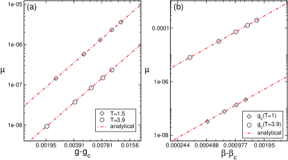
The correctness of (38) and (40) is verified in Fig. 3. The symbols in the figure are the values of $\mu$ obtained by solving (30). The dashed-dotted lines are the analytical results (38) and (40). Note that (38) and (40) hold only in the vicinity of the transition (in the figure $g-g_{c}\approx 10^{-2}$ and $\beta-\beta_{c}\approx 10^{-3}$).

Figure 4: Spherical parameter $\mu$ in the quantum spherical model at finite temperature: $3+\mu$ plotted versus $g$ at fixed temperature $T=1$. The symbols are the finite-size results for several lattice sizes $L$. Results are obtained by solving numerically the equation for the spherical constraint (20). The dashed-dotted line is the result in the thermodynamic limit. The dashed line is the analytical result for large $g$. Note that in the thermodynamic limit $\mu=0$ below the critical point at $g_{c}\approx 18.52$ (vertical dotted line). Near the critical point it is $\mu\propto(g-g_{c})^{2}$.

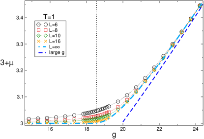
It is also useful to check how the thermodynamic limit is approached. In Fig. 4 we report numerical results for $\mu$ for finite-size systems. These are obtained by solving numerically (20). In the figure we plot $3+\mu$ versus $g$. The data are for fixed temperature $T=1$, although similar results are obtained for different temperatures. The vertical dotted line denotes the critical coupling $g_{c}$. The dashed-dotted line is the result for $\mu$ in the thermodynamic limit, i.e., obtained by solving (30). Clearly, $\mu=0$ for $g\leq g_{c}$, whereas $\mu\to\infty$ in the limit $g\to\infty$.

The different symbols are the finite-size results for $\mu$. One obtains a nonzero value for $\mu$ for any $g$. As it is clear from the figure, both in the paramagnetic and in the ferromagnetic regions the data quickly converge to the thermodynamic limit (dashed-dotted line). Around the critical point, large finite-size effects are present. The perturbative result for $\mu$ (cf. (24)) is reported in Fig. 4 as dashed-dotted line. Although the agreement is not perfect for the values of $g$ reported in the figure, we checked that the result (24) is recovered upon increasing $g$.

IV.2 Two-point correlators

By using the expansion for $\mu$ near the critical line that we derived in the previous section, it is now straightforward to obtain the two-point correlation functions. Again, the idea is to expand $\omega_{k}$ around $k=0$ in (16) and (17) in the thermodynamic limit. For the case in which the transition is approached at fixed $T$, one obtains

$$\langle s_{n}s_{m}\rangle=\frac{\sqrt{g_{c}}}{2\sqrt{2}}\int\frac{dk}{(2\pi)^{3}}\frac{\coth(\beta\sqrt{g_{c}\omega_{k}/2})}{\omega_{k}}e^{ik(n-m)}\\ +(g-g_{c})\int\frac{dk}{(2\pi)^{3}}\Big{(}\frac{\beta}{8}+\frac{\mathrm{coth}(\beta\sqrt{g_{c}\omega_{k}/2})}{4\sqrt{2g_{c}\omega_{k}}}-\frac{\beta}{8}\mathrm{coth}^{2}(\beta\sqrt{g_{c}\omega_{k}/2})\Big{)}e^{ik(n-m)}-\frac{\sqrt{2\mu}}{4\pi\beta}+{\mathcal{O}}((g-g_{c})^{2}).$$ (42)

If the critical point is approached at fixed $g$, one has

$$\langle s_{n}s_{m}\rangle=\frac{\sqrt{g}}{2\sqrt{2}}\int\frac{dk}{(2\pi)^{3}}\frac{\coth(\beta_{c}\sqrt{g\omega_{k}/2}}{\sqrt{\omega_{k}}}e^{ik(n-m)}+\\ \frac{g}{4}(\beta-\beta_{c})\int\frac{dk}{(2\pi)^{3}}\Big{(}1-\coth^{2}(\beta_{c}\sqrt{g\omega_{k}/2})\Big{)}e^{ik(n-m)}-\frac{\sqrt{2\mu}}{4\pi\beta_{c}}+{\mathcal{O}}((\beta-\beta_{c})^{2}).$$ (43)

For the correlators $\langle p_{n}p_{m}\rangle$, a similar calculation yields

$$\langle p_{n}p_{m}\rangle=\frac{1}{\sqrt{2g_{c}}}\int\frac{dk}{(2\pi)^{3}}\coth(\beta\sqrt{g_{c}\omega_{k}/2})\sqrt{\omega_{k}}e^{ik(n-m)}+\\ \frac{g-g_{c}}{g_{c}}\int\frac{dk}{(2\pi)^{3}}\omega_{k}\Big{(}\frac{\beta}{4}-\frac{\mathrm{coth}(\beta\sqrt{g_{c}\omega_{k}/2})}{2\sqrt{2\omega_{k}g_{c}}}-\frac{\beta}{4}\mathrm{coth}^{2}(\beta\sqrt{g_{c}\omega_{k}/2})\Big{)}e^{ik(n-m)}+{\mathcal{O}}((g-g_{c})^{2}).$$ (44)

If one approaches the transition along the temperature direction, one obtains

$$\langle p_{n}p_{m}\rangle=\frac{1}{\sqrt{2g}}\int\frac{dk}{(2\pi)^{3}}\coth(\beta_{c}\sqrt{g\omega_{k}/2})\sqrt{\omega_{k}}e^{ik(n-m)}+\\ \frac{1}{2}\int\frac{dk}{(2\pi)^{3}}\omega_{k}(1-\coth^{2}(\beta_{c}\sqrt{g\omega_{k}/2}))e^{ik(n-m)}(\beta-\beta_{c})+{\mathcal{O}}((\beta-\beta_{c})^{2}).$$ (45)

Clearly, in all cases (cf. (42)(43)(44) (45)) the correlation functions are finite at the critical point, and exhibit a ${\mathcal{O}}(g-g_{c})$ and ${\mathcal{O}}(\beta-\beta_{c})$ behaviour. Crucially, in both (42) and (43) one has the singular contribution $\propto\sqrt{\mu}$. On the other hand, this is not present in the expansion of $\langle p_{n}p_{m}\rangle$. This implies that the correlator $\langle s_{n}s_{m}\rangle$ has a cusp-like singularity across the critical point, whereas $\langle p_{n}p_{m}\rangle$ is regular. Finally, one should observe that the singular term in (42) and (43) does not depend on the position. This means that the spatial structure of the correlators appears only in sub-leading contributions in $g-g_{c}$ that we are neglecting.

IV.3 Scaling of the free energy

It is instructive to investigate the singular contributions to the free energy. A similar qualitative behaviour will be observed for entanglement-related quantities (see section V.2, section V.3 and section VI). Let us focus on the situation in which $T$ is kept fixed, and let us study the behaviour around the critical point as a function of $g$. At a second order phase transition the free energy density contains both analytic and singular terms. In general it can be written as vicari

$$f\equiv\frac{F}{L^{3}}=f_{\mathrm{an}}(g)+f_{\mathrm{sing}}(g).$$ (46)

The term $f_{\mathrm{an}}$ is the smooth part of the free energy, which depends analytically on the system parameters. The second part $f_{\mathrm{sing}}$ contains the singularities and the universal properties of the model. $f_{\mathrm{sing}}$ obeys the scaling form (see Ref. vicari for a review)

$$f_{\mathrm{sing}}(u_{1},u_{L},\dots,u_{n})=b^{-d}f_{\mathrm{sing}}(b^{y_{1}}u_{1},u_{L}b,\dots,b^{y_{n}}u_{n}).$$ (47)

Here $b>0$ is an arbitrary number, and $u_{n}$ are the scaling fields, which are analytic functions of the system’s parameters. $y_{n}$ are the scaling dimensions associated with the fields $u_{n}$. Here we assume that there are only two relevant scaling fields, $u_{1}$ and $u_{L}$. $u_{1}$ is associated with changing the coupling $g$, and $u_{L}$ with the finite-size scaling. $u_{L}$ has scaling dimension $y_{L}=1$. We define $y_{1}=1/\nu$. In (47), $y_{n}<0$ for $n>1$, i.e., $u_{n}$ are irrelevant, which give non-analytic scaling corrections to the free energy. Several scaling laws can be derived from (47). For instance, the finite-size scaling form of the free energy is obtained by choosing $b=1/u_{L}$. We obtain

$$f_{\mathrm{sing}}=u_{L}^{d}f_{\mathrm{sing}}(u_{1}/u_{L}^{y_{1}})$$ (48)

Using that $u_{L}\approx 1/L$, and that close to the phase transition $u_{1}\approx g-g_{c}$, we find the standard result

$$f_{\mathrm{sing}}=L^{-d}f_{\mathrm{sing}}((g-g_{c})L^{1/\nu}).$$ (49)

For a second-order phase transition, the free energy density is finite everywhere in the phase diagram. The singular part $f_{\mathrm{sing}}$ vanishes at the critical point. Indeed, for $g=g_{c}$ one obtains from (49) the contribution $f_{\mathrm{sing}}(0)L^{-3}$, which is vanishing because $f_{\mathrm{sing}}$ is finite. By choosing $u_{1}b^{y_{1}}=1$ in (47) in the thermodynamic limit one obtains the scaling behaviour

$$f_{\mathrm{sing}}=|g-g_{c}|^{d\nu}f_{\mathrm{sing}}(\mathrm{sign}(g-g_{c}))\propto|g-g_{c}|^{2-\alpha}.$$ (50)

Note the dependence on the sign of $g-g_{c}$. In (50) we used the hyperscaling relation $d\nu=2-\alpha$, with $\alpha$ the critical exponent of the specific heat. In the limit $L\to\infty$ one has to recover (50) from (49). This implies that $f_{\mathrm{sing}}((g-g_{c})L^{1/\nu})\approx|(g-g_{c})L|^{d\nu}f_{\mathrm{sing}}(\pm\infty)$ for $L\to\infty$. We should stress that in the derivations above we neglected all the scaling corrections.

It is interesting to derive the singular behaviour of the free energy in the quantum spherical model. We work in the thermodynamic limit. The density of free energy of the QSM reads (cf. (21))

$$f\equiv\lim_{L\to\infty}\frac{F}{L^{3}}=\frac{1}{\beta}\ln(2)+\frac{1}{\beta}\int\frac{dk}{(2\pi)^{3}}\ln\sinh\Big{[}\beta\sqrt{g/2}\sqrt{\mu+\omega_{k}}\Big{]}.$$ (51)

As for the spherical constraint and for the correlators (see section IV.1 and section IV.2), the idea is to expand (51) for small $k$. After expanding (51), one obtains

$$f=\frac{1}{\beta}(\ln(\beta\sqrt{g/2})+\ln(2))+\int\frac{dk}{(2\pi)^{3}}\Big{[}\frac{1}{2\beta}\ln(\mu+\omega_{k})+b_{k}(\mu,\beta,g)\Big{]},$$ (52)

where $b_{k}$ denotes an analytic function of its arguments. At the leading order it is given as

$$b_{k}\equiv\frac{\beta g}{12}(\mu+\omega_{k})+\dots$$ (53)

The leading singular behaviour is encoded in the first term in (52).

Figure 5: Density of free energy $F/L^{3}$ in the three-dimensional quantum spherical model. (a) Results obtained by using the thermodynamic value of the spherical parameter $\mu$. $F/L^{3}$ is plotted versus the quantum coupling $g$. Data are for fixed temperature $T=0.6$ and several system sizes $L$. The singular behaviour at the critical point (vertical dotted line) is unphysical (see the main text) and vanish in the thermodynamic limit. The dashed-dotted line is the result in the thermodynamic limit. (b) The same as in (a) using the finite-size value of the spherical parameter $\mu$. Data are now for $T=1$.

To extract the singularity one can use the trivial identity

$$\ln(1+z)=\int_{0}^{\infty}dt\frac{e^{-t}}{t}(1-e^{-zt}).$$ (54)

Now, the integration over $dk$ in (52) can be performed exactly to give

$$\frac{1}{2\beta}\int\frac{dk}{(2\pi)^{3}}\ln(\mu+\omega_{k})=\frac{1}{2\beta}\ln(3+\mu)+\frac{1}{2\beta}\int_{0}^{\infty}dt(1-I^{3}_{0}(t/(3+\mu)))\frac{e^{-t}}{t}.$$ (55)

Here $I_{0}$ is the modified Bessel function of the first kind. Now one can split the integration range as $[0,\infty)=[0,t_{0}]\cup[t_{0},\infty)$. For $t_{0}$ large enough, by using the asymptotic behaviour of the Bessel function $I_{0}(t)\propto e^{t}/\sqrt{2\pi t}$, one obtains

$$\int_{0}^{\infty}dt(1-I^{3}_{0}(t/(3+\mu)))\frac{e^{-t}}{t}=\int_{0}^{t_{0}}dt(1-I^{3}_{0}(t/(3+\mu)))\frac{e^{-t}}{t}+\int_{t_{0}}^{\infty}dt(1-e^{3t/(3+\mu)}/(2\pi t/(3+\mu))^{3/2})\frac{e^{-t}}{t}.$$ (56)

The singularity of the free energy is extracted from the second term in (56). In the limit $\mu\to 0$ this gives

$$\int_{t_{0}}^{\infty}dt(1-e^{3t/(3+\mu)}/(2\pi t/(3+\mu))^{3/2})\frac{e^{-t}}{t}=\Gamma(0,t_{0})-\frac{\sqrt{3/2}}{(\pi t_{0})^{3/2}}+\frac{\sqrt{3/2}(2t_{0}-1)}{2(\pi t_{0})^{3/2}}\mu-\frac{\sqrt{2}}{3\pi}\mu^{3/2}+\dots$$ (57)

Here $\Gamma(0,t_{0})$ is the incomplete Gamma function. Note that both analytic and nonanalytic terms are present in (57). The term $\mu^{3/2}$ gives the well-known singularity of the free energy in the quantum spherical model vojta

$$f_{\mathrm{sing}}=-\frac{\sqrt{2}}{6\pi}\mu^{3/2}\propto(g-g_{c})^{3},\quad\textrm{with}\,g>g_{c}.$$ (58)

From (58) we obtain $\nu=1$. The prefactor of $(g-g_{c})^{3}$ can be easily extracted from (57) and (38) (40). Eq. (58) can be also derived by observing that the spherical constraint (see section IV.1) is obtained as $\partial f/\partial\mu=V$, and by integrating with respect to $\mu$ the singular contribution in (36). From (58), one has that the specific heat exponent $\alpha=2-d\nu=-1$ is negative. Eq. (58) implies that the free energy and its first derivative with respect to $\beta$ and $g$ are continuous functions at the critical point.

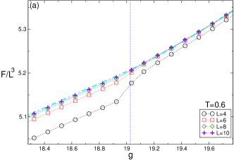
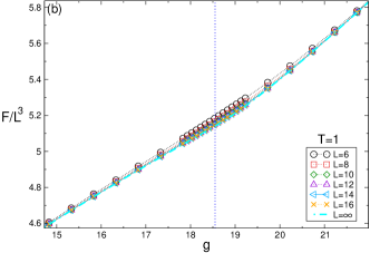
We illustrate the behaviour of the free energy across the finite temperature transition in Fig. 5. In the two panels (a) and (b) we consider two different limits. Specifically, in (a) we calculate the free energy density from the finite-size expression (21), but using the value of $\mu$ calculated in the thermodynamic limit, i.e., by solving (30). This is convenient because it is straightforward to numerically solve (30), whereas solving (20) is a nontrivial task since the sum over $k$ cannot be performed explicitly. On the other hand, since in the thermodynamic limit one has $\mu=0$ below the transition, the contribution of the zero mode in (21) is divergent and it has to be regularized by hand. The strategy that we use is to introduce a small mass putting $\mu=10^{-6}$. While this ensures that one has the correct thermodynamic limit results, it affects the sub-leading contributions. This is clear from Fig. 5 (a). In the figure we show data for $T=0.6$ and several system sizes. The data for $L=4$ show a jump at $g=g_{c}$ (vertical line). This is an artifact of the regularization. We checked that the jump becomes sharper and sharper as the mass term is sent to zero. At fixed mass, upon increasing $L$, the contribution of the zero-mode becomes negligible and the data approach the thermodynamic limit result (dashed-dotted line in the figure). Clearly, in the thermodynamic limit the free energy and its first derivative are continuous, as expected from (58). In Fig 5 (b) we show the free energy calculated by using the finite-size value of $\mu$, obtained by solving numerically (20). Now the contribution of the zero mode is finite because of the finite $L$.

IV.4 Universal ratio $R_{\xi}$

One important goal of this paper is to investigate the effectiveness of entanglement-related observables to detect finite-temperature criticality. In this section we briefly review the behaviour of the universal ratio $\xi_{\mathrm{2nd}}/L$, with $\xi_{\mathrm{2nd}}$ the second-moment correlation length. This is a standard tool used in numerical simulations to analyse criticality vicari . For instance, it allows to detect second-order phase transitions via the so-called crossing method, and it can be used to extract the critical exponent $\nu$ by the usual data collapse analysis.

Figure 6: Scaling of the second-moment correlation length at a finite-temperature phase transition in the quantum spherical model. Rescaled correlation length $\xi_{\mathrm{2nd}}/L$, with $L$ the system size, plotted as a function of $g$. The data are for fixed $T=1$ and several $L$. The vertical dotted line marks the critical point at $g_{c}\approx 18.52$. Note the crossing at $g\approx g_{c}$ between curves for different system sizes.

Figure 7: Same data as in Fig. 6 plotted versus the scaling variable $X\equiv(g-g_{c})L^{1/\nu}$, with $\nu=1$. Upon increasing $L$, the data for different $L$ collapse on the same curve. Note the large scaling corrections near the critical region at $X=0$. Inset: Zoom around $X=0$ showing only data for $L=12$-$16$. We now show results also for $T=2.2$. Note for both temperatures the same universal value $\xi_{\mathrm{2nd}}/L\approx 0.5$ at the critical point $X=0$.

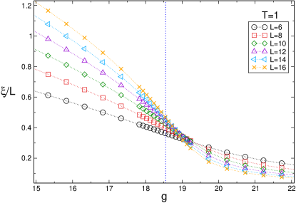
The ratio $R_{\xi}$ is defined as

$$R_{\xi}=\frac{\xi_{\mathrm{2nd}}}{L}.$$ (59)

The so-called second-moment correlation length $\xi_{\mathrm{2nd}}$ is extracted from the long-distance behaviour of the correlation function. Its definition reads

$$\xi_{\mathrm{2nd}}^{2}=\frac{\widetilde{G}(0)/\widetilde{G}(q_{\mathrm{min}})-1}{4\sin^{2}(\pi/L)},$$ (60)

with $\widetilde{G}(k)$ the Fourier transform of the spin-spin correlation function (cf. (16) for the spherical model). In (60), $q_{\mathrm{min}}$ is the minimum nonzero lattice momentum $q_{\mathrm{min}}=(2\pi/L,0,0)$. Note that $\widetilde{G}(0)$ is the spin susceptibility $\chi$ defined as

$$\chi=\frac{1}{V}\sum\limits_{n,m}\langle s_{n}s_{m}\rangle.$$ (61)

Alternatively, instead of $\xi_{\mathrm{2nd}}$, one can define $R_{\xi}$ by using $\xi_{\mathrm{gap}}$, which is defined from the gap between the ground state and the first excited state in the energy spectrum. For the quantum spherical model $R_{\xi}$ can be expressed analytically as a function of $\mu$. By using (16), one obtains that the correlation length is given as

$$\xi^{2}_{\mathrm{2nd}}=\frac{1}{4\sin^{2}(\pi/L)}\left[\frac{\alpha_{2\pi/L}^{2}\coth(\beta E_{2\pi/L}/2)}{\alpha_{0}^{2}\coth(\beta E_{0}/2)}-1\right]$$ (62)

We now discuss the finite-size scaling properties of $R_{\xi}$. The finite-size scaling ansatz for $R_{\xi}$ reads as vicari

$$R_{\xi}=K((g-g_{c})L^{1/\nu}).$$ (63)

Here we neglect both analytic and nonanalytic scaling corrections, that, however, one can include. The function $K(x)$ is universal apart from a renormalisation of its argument. Assuming analyticity of $K(x)$ one can expand (63) as

$$R_{\xi}=R^{*}_{\xi}+c_{1}(g-g_{c})L^{1/\nu}+\dots.$$ (64)

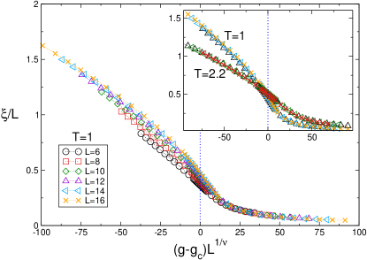
The value $R^{*}_{\xi}$ depends only on the universality class of the transition and on the geometry (for instance, the boundary conditions). Crucially, Eq. (64) implies that the curves for $R_{\xi}$ at different finite sizes $L$ exhibit a crossing at the critical point. Moreover, when plotted against the scaling variable $X\equiv(g-g_{c})L^{1/\nu}$, the data for different $L$s collapse on the same curve, at least in the limit $L\to\infty$, when corrections to scaling can be neglected.

It is important to understand the behaviour of $R_{\xi}$, especially with the moderately small system sizes that are available in our simulations. In Fig. 6 we show numerical data for $R_{\xi}$ plotted as a function of $g$. The data are for $T=1$. The curves for different $L$ exhibit a crossing at $g\approx g_{c}$, as expected. The value $R_{\xi}^{*}\approx 0.5$ at the crossing is universal, and it could be calculated by using the results of Ref. shapiro-1986, . To our knowledge $R_{\xi}^{*}$ is not known exactly. Note that scaling corrections are present. Indeed, for the smaller $L$s the crossing is not at $g_{c}$ (vertical line). Upon increasing $L$, the crossing point exhibits a systematic drifts towards $g_{c}$. In Fig. 7 we show the same data as in Fig. 6, now plotted versus the scaling variable $X=(g-g_{c})L^{1/\nu}$. As expected, due to the scaling corrections, the smaller lattice sizes do not show data collapse. However, upon increasing $L$ the quality of the collapse improves significantly. The scaling is satisfactory for the larger sizes. In the inset we provide data also for $T=2.2$. We observe that scaling corrections are smaller as compared with $T=1$, which is reflected in a better data collapse. Note that the scaling function $K$ (cf. (63)) depends on the temperature, although the value at $X=0$ is the same for both temperatures, as expected. However, since the finite-temperature universality class is the same on the whole para-ferro transition line (see Fig. 2), the two scaling functions should coincide after an analytic redefinition of the scaling field $u_{1}$ as $u_{1}\approx c_{T}(g-g_{c})$, where $c_{T}$ depends on the temperature. We numerically verified that $c_{T=2.2}/c_{T=1}\approx 1/2$.

V Entanglement scaling in the critical spherical model

We now discuss the behaviour of entanglement-motivated quantities in the finite-temperature critical QSM. Specifically, in section V.1 we briefly review how to calculate entanglement-related observables. In section V.2 we focus on the von Neumann entropy. In section V.3 we discuss the von Neumann and Rényi mutual information. In section VI we investigate the the logarithmic negativity. We consider both the negativity between two spins in an infinite system (in section VI.1), as well as the negativity between two extended adjacent blocks (in section VI.2). Finally, in section VII we focus on the single-particle entanglement spectra and negativity spectra.

V.1 Computation of entanglement-related observables in the QSM

The quantum spherical model is mappable to a system of free bosons (see section III). This implies that entanglement-related quantities are obtained from the two-point correlation functions (see Ref. viktor for a review). The key ingredients are the matrices $\mathbb{Q}_{nm}\equiv\langle s_{n}s_{m}\rangle$ and $\mathbb{P}_{nm}\equiv\langle p_{n}p_{m}\rangle$ constructed from the two-point correlation functions (cf. (16) and (17)).

Let us define the matrices $\mathbb{Q}[A]$ and $\mathbb{P}[A]$, where $n,m$ are now restricted to subsystem $A$ (see Fig. 1 (b) and (c)). The Rényi entropies of $A$ are constructed from the eigenvalues $\lambda_{j}^{2}$ of the matrix $\mathbb{Q}[A]\cdot\mathbb{P}[A]$. As it is common in the literature, we refer to the $\lambda_{j}$ as the single-particle entanglement spectrum levels. In terms of $\lambda_{j}$, the Rényi entropies are given as

$$S_{n,A}=-\frac{1}{1-n}\sum_{j}\ln\Big{[}\Big{(}\lambda_{j}+\frac{1}{2}\Big{)}^{n}-\Big{(}\lambda_{j}-\frac{1}{2}\Big{)}^{n}\Big{]}.$$ (65)

The von Neumann entropy is obtained by performing the analytic continuation $n\to 1$, which yields

$$S_{\mathrm{vN}}=\sum_{j}\Big{[}\Big{(}\lambda_{j}+\frac{1}{2}\Big{)}\ln\Big{(}\lambda_{j}+\frac{1}{2}\Big{)}-\Big{(}\lambda_{j}-\frac{1}{2}\Big{)}\ln\Big{(}\lambda_{j}-\frac{1}{2}\Big{)}\Big{]}.$$ (66)

The mutual information (see section II) is obtained by using (65) (66) and (4).

We now discuss the logarithmic negativity for a partition of $A$ as $A=A_{1}\cup A_{2}$ (see Fig. 1 (c)). One first defines the transposed matrix $\mathbb{P}[A^{T_{2}}]$ as

$$\mathbb{P}[A^{T_{2}}]\equiv\mathbb{R}[A^{T_{2}}]\mathbb{P}[A^{T_{2}}]\mathbb{R}[A^{T_{2}}].$$ (67)

Here the matrix $\mathbb{R}[A^{T_{2}}]$ acts as the identity matrix $\mathbb{I}_{A_{1}}$ on $A_{1}$ and as $-\mathbb{I}_{A_{2}}$ on $A_{2}$. The eigenvalues $\nu_{i}^{2}$ of $\mathbb{Q}[A]\cdot\mathbb{P}[A^{T_{2}}]$ form the single-particle negativity spectrum. In terms of $\nu_{i}^{2}$, the negativity is given as

$${\cal E}=\sum_{i}\textrm{max}(0,-\ln(2\nu_{i})).$$ (68)

Note that while $\nu_{i}^{2}>0$, $-\ln(2\nu_{i})$ can be both positive and negative.

V.2 Von Neumann entropy

Figure 8: Scaling of the entanglement entropy density $S_{\mathrm{vN}}/L^{3}$ at a finite-temperature quantum phase transition in the quantum spherical model. The figure shows $S_{\mathrm{vN}}/L^{3}$ as a function of $g$ for several system sizes $L$. The vertical line marks the critical point.

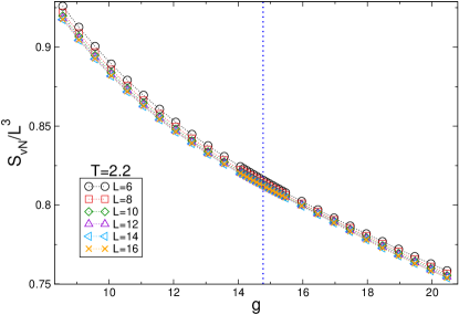
Let us start discussing the behaviour of the von Neumann entropy. Numerical data for the half-system entropy are reported in Fig. 8, for fixed temperature $T=2.2$. Similar to the free energy (see Fig. 5) and to the thermal entropy, the von Neumann entropy exhibits a volume law at any $g$. The figure shows the density of entropy $S_{\mathrm{vN}}/L^{3}$, plotted as a function of $g$. Different symbols are for different system sizes. Finite-size effects decay very quickly with $L$. The data for the larger sizes $L=12-16$ collapse on the same curve. The entropy density exhibits regular behaviour around the transition. This is expected because at finite temperature the density of von Neumann entanglement entropy becomes the same as the thermal entropy, which is not singular at the transition. We should stress, however, that sub-leading contributions can be singular, for instance due to the presence of the zero mode. A natural scaling ansatz for the entropy density reads as

$$\frac{S_{\mathrm{vN}}}{L^{3}}=L^{-3}s_{\mathrm{sing}}((g-g_{c})L^{1/\nu})+s_{\mathrm{an}}(g).$$ (69)

Here the functions $s_{\mathrm{sing}}$ and $s_{\mathrm{an}}$ encode the singular and regular terms. In (69) we neglect scaling corrections. Eq. (69) implies that the singular term vanishes at the transition when increasing $L$, and only the regular term survives. We should stress that in (69) we also neglect logarithmic contributions that can arise because of the presence of the zero mode met-grov , which reflects the symmetry breaking. We will investigate these contributions in section VII discussing the single-particle entanglement spectrum. Moreover, in principle, there can be extra logarithmic corrections if the bipartition has corners (see, for instance Ref. singh-2012, ). These are not present in our case because the boundary between $A$ and its complement is smooth (see Fig. 1).

V.3 Mutual information

Figure 9: Scaling of the density of von Neumann mutual information $I_{\mathrm{vN}}/L^{2}$ at a finite-temperature quantum phase transition in the quantum spherical model: $I_{\mathrm{vN}}/L^{2}$ as a function of $g$ for several system sizes $L$. Data are for fixed $T=2.2$. The vertical dotted line marks the critical point at $g_{c}$. Note the spurious crossing at $g<g_{c}$.

Figure 10: Scaling of the density of Rényi mutual information $I_{n}/L^{2}$ with $n=2$ at a finite-temperature phase transition: $I_{n}/L^{2}$ as a function of $g$ for several system sizes $L$. Data are for fixed $T=2.2$. The vertical dotted line marks the critical point at $g_{c}$. Inset: zoom around the critical region. Note that no crossing is present.

We now turn to the mutual information (see (4) for its definition). Here we consider a bipartite system at finite temperature (as in Fig. 1 (b)). The system is divided into two equal parts $A$ and $B=\bar{A}$. We consider the mutual information between $A$ and its complement. As it is clear from (4), the volume-law contribution of the entropies cancels out. This cancellation happens for any value of $g$ and $T$. Thus, the mutual information exhibits an area law. A natural scaling ansatz for the density of the mutual information is

$$\frac{I_{n}}{L^{2}}=L^{-2}q^{(n)}_{\mathrm{sing}}((g-g_{c})L^{1/\nu})+q^{(n)}_{\mathrm{an}}(g).$$ (70)

Eq. (70) is compatible with the scaling ansatz proposed in Ref. singh-2011, . Here $\nu$ is the critical exponent as in (69). Similar to (69), here we are neglecting scaling corrections. In (70), $q_{\mathrm{an}}$ is the analytic contribution.

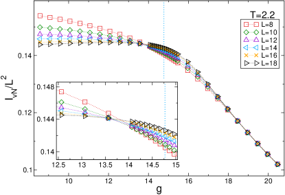
We present our results for the von Neumann mutual information $I_{\mathrm{vN}}$ in Fig. 9. We plot the density of mutual information $I_{\mathrm{vN}}/L^{2}$ versus $g$. Data are at fixed $T=2.2$. The data exhibit a crossing point around $g\approx 13.5$, which is incompatible with the critical point at $g_{c}\approx 14.77$. Moreover, the position of the crossing point does not change upon increasing system size, in contrast with the behaviour of $R_{\xi}$ (see Fig. 6). Importantly, the curves for different $L$s do not “fan out” as $L$ increases, in contrast with the behaviour for the ratio $R_{\xi}$ (see 6). As for the von Neumann entropy, the mutual information is dominated by the regular part (cf. (70)). More precisely, although the singular term in (70) gives a universal crossing, this is not visible because it is suppressed as $L^{-2}$ in the limit $L\to\infty$.

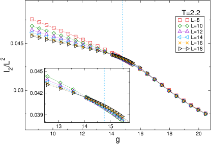
Similar behaviour is observed for the Rényi mutual information. This is discussed in Fig. 10 focusing on $I_{2}$. As for $I_{\mathrm{vN}}$, the data in Fig. 10 collapse on the same curve upon increasing $L$. Specifically, in the paramagnetic phase for $g>g_{c}$ and close to the critical point, finite-size effects decay dramatically with $L$, and the data with $L\gtrsim 10$ are already indistinguishable from the thermodynamic limit. Also no universal crossing is visible within the system sizes presented in the Figure.

It is interesting to compare our results with Ref. singh-2011, . There is large evidence, based on quantum Monte Carlo simulations, that at a finite-temperature phase transition the ratio $I_{2}/L^{d-1}$ exhibits two crossing at $T_{c}$ and $2T_{c}$, with $T_{c}$ the critical temperature. The scaling ansatz for the mutual information presented in Ref. singh-2011, is compatible with (70). However, as stressed in Ref. singh-2011, the presence of the crossing relies on $q_{\mathrm{an}}^{(n)}$ changing sign across the phase transition. Our results suggest that this does not happen in the quantum spherical model.

VI Logarithmic negativity

Figure 11: Survey of the behaviour of the logarithmic negativity in the quantum spherical model. On the $x$-axis $g$ is the quantum coupling. On the $y$-axis $T$ is the temperature. The figure shows the density plot of the half-system negativity. The system is a cube of length $L=2$. The dashed-dotted line is the critical line dividing the paramagnetic phase from the ordered phase at low temperature. The dotted line is the “death line” of the negativity. Above the death line the negativity is exactly zero. The continuous line is the death-line calculated from the negativity between two adjacent spins embedded in an infinite system. The behaviour as $\propto g^{1/2}$ at small $g$ is also reported (dashed line).

We now discuss the logarithmic negativity between two complementary subsystems. This allows us to study the interplay between genuine quantum fluctuations and thermal fluctuations. One of the goals of this section is to map out the role of entanglement in the different regions of the phase diagram of the quantum spherical model.

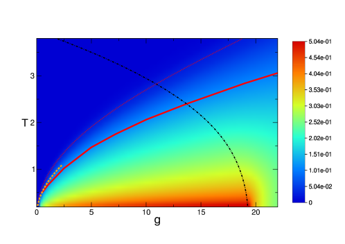
The generic behaviour of the negativity is illustrated in Fig. 11. The figure shows a density plot of ${\cal E}$ as a function of $g$ and $T$. The dashed-dotted line is the critical line dividing the paramagnetic phase from the ordered phase (see Fig. 2). In the figure we show the half-system negativity for a cube of linear size $L=2$. The data are obtained by using the value of $\mu$ in the thermodynamic limit and the finite-size formulas for the correlators (cf. (16)(17)). The negativity is large at the quantum critical point and in the ordered phase, and it quickly decays upon increasing the temperature. The dotted line is the negativity “death line”. Above the death line the half-system negativity is exactly zero. The death line that we report in the figure is obtained by considering the half-system negativity in the limit $L\to\infty$. In the figure we also report the death line calculated from the negativity between two adjacent sites embedded in an infinite system (continuous line), which provides only a bound. Interestingly, the death line exhibits the behaviour $\propto g^{1/2}$ at small $g$. For the case of two sites embedded in the infinite system the precise behaviour can be calculated analytically and it is reported in the figure (dashed line). Finally, it is interesting to observe that the death line increases with $g$, although the negativity decreases as $1/g$ (see section VI.1.1).

VI.1 Two-site negativity

Figure 12: Logarithmic negativity between two nearest-neighbour spins embedded in an infinite system. We show ${\cal E}$ along the critical $T=T_{c}(g)$ line of the para-ferro transition. Note the sudden death of the negativity at $g\approx 13.6$.

Several of the generic features of the negativity discussed in Fig. 11 can be extracted by considering two adjacent spins embedded in an infinite system. In this section we derive analytically the behaviour of the logarithmic negativity in this situation.

VI.1.1 Large $g$ expansion

It is straightforward to derive the behaviour of the negativity between the two sites in the large $g$ regime (see Fig. 2). The starting point of the analysis are the correlators $\langle s_{n}s_{m}\rangle$ and $\langle p_{n}p_{m}\rangle$ in the large $g$ limit. These are reported in (26) and (27). Now the matrices $\mathbb{Q}[A]$ and $\mathbb{P}[A^{T_{2}}]$ (see section II for their definitions) are two-by-two matrices. The negativity spectrum contains only two levels. These are the eigenvalues $\nu^{2}_{\pm}$ of $\mathbb{Q}[A]\cdot\mathbb{P}[A^{T_{2}}]$, which in the large $g$ limit are given as

$$\nu_{\pm}=\frac{g\pm 2}{2g}.$$ (71)

Since $\nu_{+}>1/2$, only $\nu_{-}$ contributes to the negativity (see (68)), which is given as

$${\cal E}=-\ln\Big{(}\frac{g-2}{g}\Big{)}.$$ (72)

By expanding in the large $g$ limit, one obtains the behaviour ${\cal E}\propto 1/g$.

VI.1.2 Low-temperature expansion

It is also interesting to discuss the limit of low-temperature in the ordered phase of the quantum spherical model. To do that, we exploit the expansion of the correlators $\langle s_{n}s_{m}\rangle$ and $\langle p_{n}p_{m}\rangle$ (cf. (28) and (29)). Let us first consider the negativity between site $n\equiv(n_{x},n_{y},n_{z})$ and $m\equiv(m_{x},m_{y},m_{z})$. The eigenvalues $\nu_{i}^{2}$ of $\mathbb{Q}[A]\cdot\mathbb{P}[A^{T_{2}}]$ are given as

$$\nu_{1}^{2}=\frac{(W^{\prime\prime}_{n}-W^{\prime\prime}_{m})(\sqrt{2}+3(W^{\prime}_{n}+W^{\prime}_{m})\beta^{2}g)}{12\beta^{2}g},$$ (73)

$$\nu_{2}^{2}=\frac{(W^{\prime}_{n}-W^{\prime}_{m})(\sqrt{2}\pi^{2}+15(W^{\prime\prime}_{n}+W^{\prime\prime}_{m})\beta^{4}g)}{60\beta^{4}g^{2}}.$$ (74)

Here we defined the Watson-type integrals $W_{n}^{\prime}$ as

$$W_{n}^{\prime}\equiv\int\frac{dk}{(2\pi)^{3}}e^{ikn}\frac{1}{\sqrt{\omega_{k}}},\quad W_{n}^{\prime\prime}\equiv\int\frac{dk}{(2\pi)^{3}}e^{ikn}\sqrt{\omega_{k}}.$$ (75)

Here $\omega_{k}$ is defined in (12). Interestingly, the integral $W^{\prime}_{n}$ can be calculated analytically in terms of hypergeometric functions guttmann-2010 . We now restrict ourselves to the negativity between two nearest-neighbour spins, i.e., with $|n-m|=1$. Specifically, we choose $n=(0,0,0)$ and $m=(1,0,0,)$. One can numerically check that $\nu_{1}^{2}<1/4$, implying that $\nu_{1}$ does not contribute to the negativity (see (68)). On the other hand, for a given $\beta$, one has that $\nu_{2}$ contributes to the negativity only for sufficiently large $g$. Specifically, we observe that the condition $g>g^{*}(\beta)$ has to hold, with the ”critical” value $g^{*}$ given as

$$g^{*}=\frac{2^{1/4}\pi\sqrt{W^{\prime}_{0}-W^{\prime}_{1}}}{\sqrt{15}\beta^{2}\sqrt{1-(W^{\prime}_{0}-W^{\prime}_{1})(W^{\prime\prime}_{0}+W^{\prime\prime}_{1})}},$$ (76)

where $W^{\prime}_{0}\equiv W^{\prime}_{(0,0,0)},W^{\prime}_{1}\equiv W^{\prime}_{(1,0,0)}$, and similarly for $W^{\prime\prime}$. For each value of temperature, the negativity is exactly zero for $g<g^{*}(T)$. Note in (76) the behaviour $g^{*}\propto 1/\beta^{2}$. This behaviour persists when considering the negativity between two extended systems, although the prefactor in (76) is different. In particular, for two extended systems one obtains a larger value of $g^{*}$ in (76), as it is clear from Fig. 11.

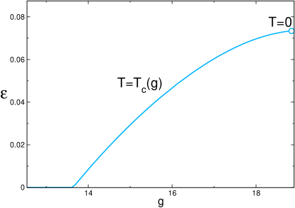
Note that for large enough temperature the negativity vanishes even on the critical line (see Fig. 2). This is shown explicitly in Fig. 12. The figure shows ${\cal E}$ calculated on the critical line $T_{c}(g)$, with $T_{c}$ the critical temperature at the given value of $g$. The negativity is exactly zero for $g\lesssim 14$, whereas it is finite nonzero up to $g\approx 19$, which corresponds to zero temperature.

Figure 13: Logarithmic negativity between two adjacent spins in the quantum spherical model: Negativity ${\cal E}$ plotted as a function of $g$ (in (a)) and of the temperature $T$ (in (b)). The figure shows results in the thermodynamic limit. The vertical lines denote the critical point. Data in (a) are for fixed $T=1$. In (b) we fixed $g=g(T_{c}=1)$ (see Fig. 2). Note in (a) the slow decay at $g\to\infty$ and the “death” of ${\cal E}$ at $g\to 0$. Note that in (b) the negativity is identically zero for $T\gtrsim 3$.

The behaviour of the negativity between two nearest-neighbour sites as a function of both temperature and quantum coupling $g$ is summarized in Fig. 13. Panel (a) shows ${\cal E}$ versus $g$, at fixed $T=1$. In the figure we plot the negativity and not its density. The vanishing behaviour below $g^{*}\approx 2$, as predicted by Eq. (76), is clearly visible, as well as the slow decay as $1/g$ in the paramagnetic phase. Panel (b) shows ${\cal E}$ at fixed $g=g_{c}(T=1)$ as a function of $T$. The negativity exhibits a weak dependence on temperature in the ordered phase, whereas it suddenly drops to zero in the paramagnetic phase (sudden death).

VI.1.3 Critical region

An important feature in Fig. 13 (a) is that the negativity exhibits regular behaviour across the para-ferro transition. On the other hand, recently it has been observed that the negativity can exhibit a cusp-like singularity at a finite temperature phase transition tarun-1 ; tarun-2 . Moreover, it has been suggested that the singular part of the negativity obeys the scaling form as

$${\cal E}_{\mathrm{sing}}\propto|g-g_{c}|^{1-\alpha},$$ (77)

with $\alpha$ the specific heat critical exponent. Our results are consistent with Ref. tarun-1, ; tarun-2, . Specifically, for the $3D$ QSM one has $\alpha=-1$. Thus, Eq. (77) predicts that ${\cal E}_{\mathrm{sing}}$ has a singular term $(g-g_{c})^{2}$, i.e., a weaker than a cusp singularity. On the other hand, for $\alpha=0$, which is the case investigated in Ref. tarun-2, , one has the cusp-like behaviour as ${\cal E}_{\mathrm{sing}}\propto|g-g_{c}|$.

To clarify the behaviour of ${\cal E}$ for two nearest-neighbour sites, it is useful to consider the single-particle negativity spectrum. Using the expansions for the correlators near the critical point (cf. (43)(42)(44), and (45)), it is straightforward to obtain the spectrum levels. These are given as

$$\nu_{1}^{2}=(S_{nn}^{(0)}-S_{nm}^{(0)})(P_{nn}^{(0)}+P_{nm}^{(0)})+\big{[}(S_{nn}^{(1)}-S_{nm}^{(1)})(P_{nn}^{(0)}+P_{nm}^{(0)})+(S_{nn}^{(0)}-S_{nm}^{(0)})(P_{nn}^{(1)}-P_{nm}^{(1)})\big{]}(g-g_{c}),$$ (78)

$$\nu_{2}^{2}=(S_{nn}^{(0)}+S_{nm}^{(0)})(P_{nn}^{(0)}-P_{nm}^{(0)})+\big{[}(S_{nn}^{(1)}+S_{nm}^{(1)}+2Z_{\mathrm{sing}})(P_{nn}^{(0)}-P_{nm}^{(0)})+(S_{nn}^{(0)}+S_{nm}^{(0)})(P_{nn}^{(1)}+P_{nm}^{(1)})\big{]}(g-g_{c}).$$ (79)

Here we defined

$$S_{nm}^{(0)} \equiv\frac{\sqrt{g_{c}}}{2\sqrt{2}}\int\frac{dk}{(2\pi)^{3}}\frac{\coth(\beta\sqrt{g_{c}\omega_{k}/2})}{\sqrt{\omega_{k}}}e^{ik(n-m)}$$ (80)

$$S_{nm}^{(1)} \equiv\int\frac{dk}{(2\pi)^{3}}\Big{(}\frac{\beta}{8}+\frac{\mathrm{coth}(\beta\sqrt{g_{c}\omega_{k}/2})}{4\sqrt{2g_{c}\omega_{k}}}-\frac{\beta}{8}\mathrm{coth}^{2}(\beta\sqrt{g_{c}\omega_{k}/2})\Big{)}e^{ik(n-m)}$$ (81)

$$P_{nm}^{(0)} \equiv\frac{1}{\sqrt{2g_{c}}}\int\frac{dk}{(2\pi)^{3}}\coth(\beta\sqrt{g_{c}\omega_{k}/2})\sqrt{\omega_{k}}e^{ik(n-m)}$$ (82)

$$P_{nm}^{(1)} \equiv\frac{1}{g_{c}}\int\frac{dk}{(2\pi)^{3}}\omega_{k}\Big{(}\frac{\beta}{4}-\frac{\mathrm{coth}(\beta\sqrt{g_{c}\omega_{k}/2}}{2\sqrt{2g_{c}\omega_{k}}}-\frac{\beta}{4}\mathrm{coth}^{2}(\beta\sqrt{g_{c}\omega_{k}/2})\Big{)}e^{ik(n-m)}$$ (83)

$$Z_{\mathrm{sing}} \equiv 2\sqrt{2}\pi\beta\int\frac{dk}{(2\pi)^{3}}\Big{(}\frac{\beta}{8}+\frac{\mathrm{coth}(\beta\sqrt{g_{c}\omega_{k}/2})}{4\sqrt{2g_{c}\omega_{k}}}-\frac{\beta}{8}\mathrm{coth}^{2}(\beta\sqrt{g_{c}\omega_{k}/2})\Big{)}$$ (84)

Figure 14: Single-particle negativity spectrum for two adjacent spins the embedded in an infinite system. We plot $-\ln(2\nu_{n})$, with $\nu_{n}^{2}$ the eigenvalues of the correlation matrix, versus $g$. Data are for fixed $T\approx 1.486$. The spectrum consists of two eigenvalues shown in (a) and (b). Note that in (b) $-\ln(2\nu_{n})<0$, implying that the level does not contribute to the negativity. Note the kink at the critical point (vertical line). In contrast, the eigenvalue in (a) is regular, implying that the negativity is not singular at the critical point.

Note that $Z_{\mathrm{sing}}$ contains the singular term $\sqrt{\mu}$ that we derived in section IV.1. Interestingly, this affects only $\nu_{2}$, whereas $\nu_{1}$ is regular.

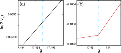
In Fig. 14 we show the levels of the single-particle negativity spectrum (cf. (80) and (81)). In the figure we plot $-\ln(2\nu_{n})$ versus $g$. In (a) we show the regular eigenvalue $\nu_{1}$, whereas $\nu_{2}$ is reported in (b). The singularity as $|g-g_{c}|$ in (b) is clearly visible. Importantly, one has that $-\ln(2\nu_{2})<0$, implying that $\nu_{2}$ does not contribute to the logarithmic negativity. This suggests that in the case of two extended subsystems only a subset of the single-particle negativity spectrum levels will exhibit singular behaviour. These levels, however, do not contribute to the negativity, which is regular at the finite-temperature transition. This point will be better clarified when we will discuss the negativity spectrum of two extended regions in section VII.

VI.2 Half-system negativity

Figure 15: Logarithmic negativity in the finite-temperature quantum spherical model. (a) and (b) show the negativity density ${\cal E}/L^{2}$ plotted versus the quantum coupling $g$ for $T=1$ and $T=0.2$, respectively. Data are obtained by using the thermodynamic result for the spherical constraint $\mu$. The effect of the system size $L$ is small, especially for $T=1$. The qualitative behaviour is similar to Fig. 13 (compare (a) and (b)). For $T=1$ the negativity exhibits regular behaviour at $g_{c}$, whereas in the limit $T\to 0$ a cusp-like feature appears at $g_{c}$. In (b) the inset shows the data for $L=10$, zooming around the critical point.

We now discuss the half-system logarithmic negativity. Our results are reported in Fig. 15. The figure provides an overview of ${\cal E}$ at fixed temperature $T=1$ and $T=0.2$ ((a) and (b), respectively) as a function of $g$. In both panels we plot the negativity density ${\cal E}/L^{2}$ of half system. The different lines are for different sizes $L$. Similar to section IV.3, we calculate the negativity by using the finite-size result for the correlators (see (16) and (17)), and the value of the spherical parameter $\mu$ in the thermodynamic limit. To regularize the divergent contribution of the zero mode we fix $\mu=10^{-6}$ for $g\leq g_{c}$. We also checked that the results for the negativity do not depend on the choice of the regularization.

Clearly, in Fig. 15 finite-size effects are small, especially for $T=1$ (see (a)). In (a) the data for $L=8$ cannot be distinguished from the result in the thermodynamic limit. In both (a) and (b), the negativity has its maximum value at the critical point. In the paramagnetic phase the negativity decays as $1/g$, similar to the case of two spins (see section VI.1). Within the ordered phase ${\cal E}$ exhibits a mild dependence on $g$, except at small $g$, where it drops dramatically. Specifically, for $g<g^{*}\approx 2$ the negativity is exactly zero. Note that $g^{*}$ decreases with decreasing the temperature (compare (a) and (b) in the figure). This behaviour is similar to what observed for the two-site negativity (see Fig. 13). Again, this implies that for any value of the temperature there is a “critical” value of the coupling $g$ below which the quantum fluctuations are not strong enough to give a finite entanglement negativity. An important remark, however, is that since the negativity gives only a bound on the entanglement, the vanishing of ${\cal E}$ below $g^{*}$ does not imply the absence of entanglement. From Fig. 15 (a) it is clear that at $T=1$, the negativity exhibits regular behaviour at $g_{c}$. On the other hand, upon decreasing the temperature the negativity develops a cusp. This is clear from Fig. 15 (b). Similar (weak) singular behaviour was observed in the area-law prefactor of the von Neumann entropy in ground-state quantum phase transitions kallin-2013 ; helmes-2014 ; frerot-2016 .

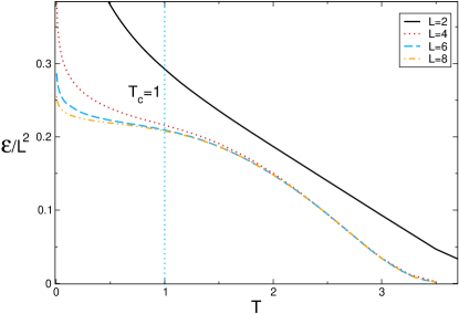
It is interesting to investigate the behaviour of the logarithmic negativity at fixed $g$, i.e., approaching criticality by changing the temperature. This is illustrated in Fig. 16. We plot ${\cal E}/L^{2}$ versus $T$ for fixed $g=g_{c}(T=1)$. Now the negativity exhibits a fast decay with $T$ in the paramagnetic region, and already for $T\approx 3$ it is exactly zero. This is in contrast with the result at fixed $T$ (see Fig. 15), where the behaviour as $1/g$ is observed. Finite-size effects are larger upon decreasing the temperature in the ordered phase. Note that for the smaller system sizes one has a quite large value of ${\cal E}$ in the limit $T\to 0$, although the area-law behaviour ${\cal E}\propto L^{2}$ is expected to hold also at zero temperature. Finally, the negativity is not singular at the critical point, as in Fig. 15.

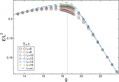
Finally, we investigate the behaviour of the logarithmic negativity in finite-size systems. To address this point, we provide results for the half-system negativity obtained by using the finite-size value of the spherical parameter $\mu$, i.e., by numerically solving (20). Our results are reported in Fig. 17. The figure plots the negativity density ${\cal E}/L^{2}$ versus $g$, for several sizes (symbols in the figure). Similar to the mutual informations (cf. Fig. 9 and 10), the data show small finite-size effects both in the paramagnetic phase and in the ordered phase. At the critical point (vertical line) finite-size effects are larger. However, the data appear to converge to the thermodynamic limit result (dashed-dotted line). The latter is obtained from Fig. 15. Note that the data for different $L$s do not exhibit any crossing at the critical point.

Figure 16: Density of the logarithmic negativity ${\cal E}/L^{2}$ in the three-dimensional quantum spherical model at fixed $g_{c}\approx 18.52$ plotted as a function of temperature $T$. Data are obtained by using the value of the spherical parameter $\mu$ in the thermodynamic limit. The vertical line is the critical temperature $T_{c}=1$ at $g_{c}$ (see Fig. 2). Note that ${\cal E}=0$ for $T\gtrsim\approx 3.5$. In the limit $T\to 0$ quantum fluctuations are enhanced and ${\cal E}/L^{2}$ increases, although area-law ${\cal E}\propto L^{2}$ behaviour should persist even at zero temperature.

Figure 17: Scaling of the negativity ${\cal E}$ at a finite-temperature quantum phase transition in the quantum spherical model. We plot ${\cal E}/L^{2}$ versus $g$. The results are at fixed $T=1$. Different symbols are for different sizes $L$. Data are obtained by solving the finite-size constraint equation (20). The vertical dotted line marks the critical point at $g_{c}\approx 18.52$. The dashed-dotted line is the result in the thermodynamic limit. Note the larger finite-size effects in the critical region.

VII Entanglement spectra, negativity spectra, and the zero mode

Figure 18: Single-particle entanglement spectrum between two adjacent blocks embedded in an infinite system. The figure shows the single-particle entanglement spectrum levels $\lambda_{n}^{2}$. The results are at the critical point at $g_{c}\approx 12.77$. Subsystem $A$ consists of a cube of size $\ell$. Different symbols are for different $\ell$. A logarithmic scale is used on the $y$-axis. Inset: $\delta_{n}\equiv(\lambda_{n}^{2})^{\prime}_{+}-(\lambda_{n}^{2})^{\prime}_{-}$, with $(\lambda_{n}^{2})^{\prime}_{\pm}$ the left and right derivative of $\lambda_{n}^{2}$ with respect to $g$ calculated at $g_{c}$. Data are for $\ell=6$. Note that $\delta_{n}\neq 0$ only for a small subset of levels.

Figure 19: Single-particle negativity spectrum between two adjacent blocks embedded in an infinite system. The figure shows the single-particle negativity spectrum levels $\nu_{n}^{2}$. Subsystem $A$ is a cube of size $\ell$. $A_{1}$ and $A_{2}$ are the two halves of the cube of linear sizes $\ell_{x}=\ell/2,\ell_{y}=\ell,\ell_{z}=\ell$ (see Fig. 1 (c)). The results are at the critical point at $g_{c}\approx 12.77$. Note that only the levels $\nu_{n}^{2}<1/4$ (horizontal dashed line) contribute to the logarithmic negativity. Inset: $\delta_{n}\equiv(\nu_{n}^{2})^{\prime}_{+}-(\nu_{n}^{2})^{\prime}_{-}$, with $(\nu_{n}^{2})^{\prime}_{\pm}$ the left and right derivative of $\nu_{n}^{2}$ with respect to $g$ at the critical point $g_{c}$. Note that $\delta_{n}=0$ for large $n$, i.e., for the levels that contribute to the negativity.

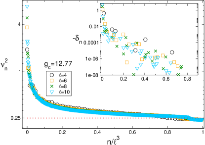
In section VI.1.3 we showed that the negativity spectrum for two nearest-neighbor sites contains one regular and one singular levels. The latter exhibits a cusp-like singularity across the finite temperature transition. The singular level, however, does not contribute to the logarithmic negativity. Moreover, we observed in section VI.2 that the negativity between two extended blocks shows regular behaviour across the transition, similar to the entanglement entropy (see Fig. 8). It is interesting to investigate how this is reflected in the negativity spectrum of two extended regions. It is also interesting to compare the singularity structure of the negativity spectrum and the entanglement spectrum.

VII.1 Entanglement spectra

Let us start discussing the entanglement spectrum. Let us consider the two matrices $\mathbb{Q}_{nm}=\langle s_{n}s_{m}\rangle$ and $\mathbb{P}_{nm}=\langle p_{n}p_{m}\rangle$ (see section II). Here we work in the thermodynamic limit. Since we are interested in the cusp-like singularity of the entanglement spectrum, it is convenient to expand $\mathbb{Q}$ and $\mathbb{P}$ as

$$\mathbb{Q}=\mathbb{Q}_{0}+(g-g_{c})\mathbb{Q}_{1}^{\pm}+\dots$$ (85)

$$\mathbb{P}=\mathbb{P}_{0}+(g-g_{c})\mathbb{P}_{1}+\dots,$$ (86)

where the dots denote higher order terms in powers of $g-g_{c}$, which we neglect. The matrices $\mathbb{Q}_{0}$ and $\mathbb{P}_{0}$ are obtained from $S_{nm}^{(0)}$ and $P_{nm}^{(0)}$ (cf. (80) and (82)), whereas $\mathbb{Q}_{1}$ and $\mathbb{P}_{1}$ are easily derived from $S_{nm}^{(1)}$ and $P_{nm}^{(1)}$ (see (81) and (83)). The $\pm$ in $\mathbb{Q}_{1}^{\pm}$ is to stress that the matrix is different on the two sides of the transition, because of the term $Z_{\mathrm{sing}}$ (see (84)), which is only present for $g>g_{c}$. We now have at the leading order ${\mathcal{O}}(g-g_{c})$

$$\mathbb{Q}\cdot\mathbb{P}=\mathbb{Q}_{0}\cdot\mathbb{P}_{0}+(g-g_{c})(\mathbb{Q}_{0}\cdot\mathbb{P}_{1}+\mathbb{Q}_{1}^{\pm}\cdot\mathbb{P}_{0})+\dots$$ (87)

By using standard perturbation theory, one obtains that the corrections to the eigenvalues $\lambda_{n}^{2}$ of the matrix $\mathbb{Q}_{0}\cdot\mathbb{P}_{0}$ are given as

$$\delta\lambda_{n}^{2}=(g-g_{c})\langle\phi_{n}|\mathbb{Q}_{0}\cdot\mathbb{P}_{1}+\mathbb{Q}_{1}^{\pm}\cdot\mathbb{P}_{0}|\phi_{n}\rangle,$$ (88)

where $|\phi_{n}\rangle$ is the eigenvector of $\mathbb{Q}_{0}\cdot\mathbb{P}_{0}$ corresponding to eigenvalue $\lambda_{n}^{2}$. Clearly, the singularity in the negativity is determined by the second term in (88), which depends on $Z_{\mathrm{sing}}$. Now we observe that $Z_{\mathrm{sing}}$ does not depend on the positions $n,m$. This has striking consequences for the single-particle entanglement spectrum. First, the singular contribution in (88) is given as

$$[\delta\lambda_{n}^{2}]_{\mathrm{sing}}=(g-g_{c})Z_{\mathrm{sing}}\langle\phi_{n}|(1,1,\dots)\otimes(1,1,\dots)\cdot\mathbb{P}|\phi_{n}\rangle.$$ (89)

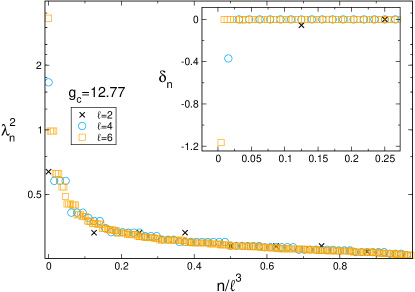
Note that the vector $(1,1,\dots)\otimes(1,1,\dots)\cdot\mathbb{P}|\phi_{n}\rangle$ is flat, i.e, all the elements are equal. Moreover, we numerically observed that the eigenvector $|\phi_{0}\rangle$ is approximately flat, i.e., all its components are $1/\ell^{3/2}$, which reflects the presence of a zero mode. This implies that for $n=0$ the expectation value in (89) is nonzero. On the other hand, the components of $|\phi_{n}\rangle$ with $n>0$ are real and are orthogonal to $|\phi_{0}\rangle$. This implies that the expectation value in (89) approximately vanishes for $n>0$. This allows us to conclude that the only few spectrum levels are singular across the transition, i.e., the ones related to the zero mode. We summarize our results in Fig. 18. The figure shows the single-particle entanglement spectrum levels $\lambda_{n}^{2}$. Here subsystem $A$ is the cube of size $\ell$ (see Fig. 1 (c)) embedded in an infinite system. One has that $\lambda^{2}_{n}>1/4$ $\forall n$. The eigenvalues $\lambda_{n}^{2}$ quickly decay with their index $n$. For most of the eigenvalues, one has $\lambda_{n}^{2}\approx 1/4$. In the inset of Fig. 18 we plot $\delta_{n}$ defined as

$$\delta_{n}\equiv(\lambda_{n}^{2})^{\prime}_{+}-(\lambda_{n}^{2})^{\prime}_{-}.$$ (90)

Here $(\lambda_{n}^{2})^{\prime}_{\pm}$ are the right and left derivatives with respect to $g$ of $\lambda_{n}^{2}$, calculated at $g_{c}$. A nonzero value of $\delta_{n}$ signals that the level $\lambda_{n}$ is singular across the transition. The results in the figure are obtained by using (89). Clearly, one has that $\delta_{n}\neq 0$ only for small $n$.

VII.2 Negativity spectra

We now discuss the negativity spectrum. Subsystem $A$ is now divided into two parts $A_{1},A_{2}$ of sizes $\ell_{x}=\ell/2,\ell_{y}=\ell,\ell_{z}=\ell$ (see Fig. 1 (c)). The partial transposition is performed with respect to $A_{2}$. Our results for the negativity spectrum are shown in Fig. 19. In the main figure we show the eigenvalues $\nu_{n}^{2}$ of the matrix $\mathbb{Q}_{0}\cdot\mathbb{P}_{0}[A^{T_{2}}]$ versus $n/\ell^{3}$. For most of the eigenvalues one has that $\nu_{n}^{2}>1/4$, implying that they do not contribute to the negativity (see section V.1). As for the entanglement spectrum, the flat vector is an approximate eigenvector of $\mathbb{Q}_{0}\cdot\mathbb{P}_{0}[A^{T_{2}}]$, with eigenvalue $\nu_{0}^{2}$. For instance, we numerically checked that for $\ell=4,6$ the eigenvector associated with $\nu_{0}^{2}$ has components are in the interval $[-0.15,-0.10]$, clustering around the expected value $1/\ell^{3/2}=0.125$. This behaviour is reflected in that of $\delta_{n}$. The definition of $\delta_{n}$ is the same as in (90) after replacing $\lambda_{n}\to\nu_{n}$. Clearly, the expansions (85) also hold upon replacing $\mathbb{P}_{0}\to\mathbb{P}_{0}[A^{T_{2}}]$ and $\mathbb{P}_{1}\to\mathbb{P}_{1}[A^{T_{2}}]$. For each negativity spectrum level, $\delta_{n}$ is plotted in the inset in Fig. 19. In contrast with the entanglement spectrum (compare with Fig. 18), one has $\delta_{n}\neq 0$ for a large subset of levels at small $n$. For instance, for $\ell=6$ one has $\delta_{n}=0$ only for $n\gtrsim 10$. As it is clear from Fig. 18 all the levels of the negativity spectrum with $\delta_{n}\neq 0$ do not contribute to the negativity because they correspond to $\lambda_{n}^{2}>1/4$. This suggests a suppression of the logarithmic correction to the boundary-law scaling of the logarithmic negativity, in contrast with the entanglement entropy (see section VII.1).

VIII Conclusions

We investigated the interplay between entanglement and classical fluctuations at finite-temperature critical points. Specifically, we focused on the three dimensional quantum spherical model, which has a finite-temperature transition between a paramagnetic phase and a ferromagnetically ordered phase. We considered several entanglement-related observables, such as the von Neumann and Rényi entropies, the mutual information, and the logarithmic negativity. In particular, we characterized the behaviour of the logarithmic negativity in all the different phases and at the transition. We also investigated how the behaviour of the entropies and of the negativity is reflected in the single-particle entanglement spectrum and on the negativity spectrum.

We now mention several important directions for future research. First, it would be important to explore the behaviour of entanglement-related observables in different dimensions. For instance, in $d=4$ the para-ferro transition becomes mean field. It would be interesting to investigate how this is reflected in the singularity structure of entanglement. An interesting direction is to investigate the logarithmic negativity at the quantum phase transition in $d=3$. Our results suggest that the logarithmic negativity exhibits a cusp-like singularity. It would be useful to understand how this is reflected in the structure of the negativity spectrum. Another interesting direction is to study the crossover from quantum to classical criticality. Moreover, it would be enlightening to generalize the perturbative analysis developed in section VII including higher-order corrections. This would allow, in principle, to characterise the full singularity structure of entanglement-related quantities.

It would be also useful to extend our analysis to other entanglement-related quantities, such as the quantum Fisher information, especially in the light of the results of Ref. hauke-2016, . Interestingly, the quantum spherical model remains exactly solvable even in the presence of long-range interactions. This opens the possibility of studying entanglement-related quantities in long-range models.

Another important direction is to study the out-of-equilibrium dynamics of entanglement-related quantities after a quantum quench. In recent years, it has been shown CCsemiclassics ; FaCa08 ; AlCa17 ; AlCa17a that for integrable models it is possible to describe quantitatively the entanglement dynamics by combining integrability with a quasiparticle picture. It would be interesting to investigate the validity of this picture for $d>1$. In $d=3$ this could also allow to investigate whether the presence of finite-temperature criticality affects the entanglement dynamics. Finally, it has been suggested in Ref. gge-mf that in the $O(N)$ model with $N\to\infty$ the steady-state arising after a quantum quench is not described by the so-called Generalized Gibbs Ensemble. The quantum spherical model provides an ideal framework to clarify this issue.

IX Acknowledgements

We thank F. Parisen Toldin for several useful discussions. VA acknowledges support from the D-ITP consortium, a program of the NWO, and from the European Research Council under the ERC Advanced grant 743032 DYNAMINT.

Appendix A Evaluation of some Watson-type integrals

The numerical evaluation of the three-dimensional integrals appearing in the expression for the correlators in (16) is a demanding task. However, there are well-known tricks to reduce them to one-dimensional integrals. To proceed we imagine of expanding the integrand in (16) in the limit $k\to 0$. Thus, one obtains that the first term is $\propto 1/\omega_{k}$. The higher-order terms yield integrals of the type $\int dk/(2\pi)^{3}\omega_{k}^{\alpha}$, with $\alpha$ a positive integer. These integrals can be performed analytically by exploiting the fact that series-2000

$$\int_{-\pi}^{\pi}\frac{dk}{(2\pi)^{3}}e^{ikx}\big{(}-\sum_{j=x,y,z}\cos k_{j}\big{)}^{\alpha}=\\ \left\{\begin{array}[]{cc}0&\textrm{if}\,\alpha=0,\dots,X-1\\ (-1)^{\alpha}\alpha!2^{-|x_{1}|-|x_{2}|-|x_{3}|}\sum_{p_{1},p_{2},p_{3}\geq 0}2^{-2p_{1}-2p_{2}-2p_{3}}\frac{\delta_{p_{1}+p_{2}+p_{3},(\alpha-X)/2}}{p_{1}!p_{2}!p_{3}!(p_{1}+|x_{1}|)!(p_{2}+|x_{2}|)!(p_{3}+|x_{3}|)!}&\textrm{if}\,\alpha-X\geq 0,\alpha-X\textrm{even}.\end{array}\right.$$ (91)

Here we defined $X\equiv|x_{1}|+|x_{2}|+|x_{3}|$. Clearly, the integral of $\omega_{k}^{\alpha}$ can be obtained by using Eq. (91) and Newton’s binomial formula. We now discuss the integration of the singular contribution. The resulting integral is of the type

$$\int\frac{dk}{(2\pi)^{3}}e^{ik(n-m)}\omega_{k}^{-1}.$$ (92)

The integral (92) can be rewritten as a one-dimensional integral. One can use the identity

$$\frac{1}{1+z}=\int_{0}^{\infty}dte^{-(z+1)t}.$$ (93)

After using (93) in (92), the integration over $k$ can be performed explicitly. One obtains

$$\int\frac{dk}{(2\pi)^{3}}\frac{e^{ik(n-m)}}{\omega_{k}}=\int_{0}^{\infty}dte^{-3t}I_{n_{x}-m_{x}}(t)I_{n_{y}-m_{y}}(t)I_{n_{z}-m_{z}}(t),$$ (94)

where $I_{\alpha}(x)$ are the Bessel functions of the first kind. The integral in (94) can be efficiently evaluated numerically.

References

- (1) J. Eisert, M. Cramer, and M. B. Plenio, Colloquium: Area laws for the entanglement entropy, Rev. Mod. Phys. 82, 277 (2010).
- (2) L. Amico, R. Fazio, A. Osterloh, V. Vedral, Entanglement in many-body systems, Rev. Mod. Phys. 80, 517 (2008).
- (3) P. Calabrese, J. Cardy, and B. Doyon, Introduction to ’Entanglement entropy in extended quantum systems, J. Phys. A 42 500301 (2009).
- (4) N. Laflorencie, Quantum entanglement in condensed matter systems, Phys. Repts. 646, 1 (2016).
- (5) M. M. Wolf, Violation of the Entropic Area Law for Fermions, Phys. Rev. Lett. 96, 010404 (2006).
- (6) D. Gioev and I. Klich, Entanglement Entropy of Fermions in Any Dimension and the Widom Conjecture, Phys. Rev. Lett. 96, 100503 (2006).
- (7) P. Calabrese, M. Mintchev, and E. Vicari, Entanglement entropies in free fermion gases for arbitrary dimension, Europhys. Lett. 97, 20009 (2012).
-
(8)
J. Lee, M. S. Kim, Y. J. Park, and S. Lee,
Partial teleportation of entanglement in a noisy environment,
J. Mod. Opt. 47, 2151 (2000);
J. Eisert and M. B. Plenio, A comparison of entanglement measures, J. Mod. Opt. 46, 145 (1999). - (9) G. Vidal and R. F. Werner, Computable Measure of Entanglement, Phys. Rev. A 65, 032314 (2002).
(10)
M. B. Plenio, Logarithmic Negativity: A Full Entanglement Monotone That is not Convex,
Phys. Rev. Lett. 95, 090503 (2005);
J. Eisert, Entanglement in quantum information theory, quant-ph/0610253. - (11) P. Calabrese, J. Cardy, and E. Tonni, Entanglement Negativity in Quantum Field Theory, Phys. Rev. Lett. 109, 130502 (2012).
- (12) P. Calabrese, J. Cardy, and E. Tonni, Finite temperature entanglement negativity in conformal field theory, J. Phys. A 48, 015006 (2015).
- (13) C. De Nobili, A. Coser, and E. Tonni, Entanglement negativity in a two dimensional harmonic lattice: area law and corner contributions, J. Stat. Mech. (2016) 083102.
- (14) V. Eisler and Z. Zimboras, Entanglement negativity in two-dimensional free lattice models, Phys. Rev. B 93, 115148 (2016).
- (15) H. Shapourian and S. Ryu, Finite-temperature entanglement negativity of Fermi surface, arXiv:1807.09808.
- (16) T.-C. Lu and T. Grover, Singularity in entanglement negativity across finite-temperature phase transitions, Phys. Rev. B 99, 075157 (2019).
- (17) T.-C. Lu and T. Grover, Structure of Quantum Entanglement at a Finite Temperature Critical Point, arXiv:1907.01569.
- (18) R. Nandkishore, D. A. Huse, Many-Body Localization and Thermalization in Quantum Statistical Mechanics, Annual Review of Condensed Matter Physics, 6 15 (2015).
- (19) V. Khemani, S. P. Lim, D. N. Sheng, and D. Huse, Critical Properties of the Many-Body Localization Transition, Phys. Rev. X 7, 021013 (2017).
- (20) J. Kjall, J. Bardarson, and F. Pollmann, Many-Body Localization in a Disordered Quantum Ising Chain, Phys. Rev. Lett. 113, 107204 (2014).
- (21) A. Chandran, C. R. Laumann, and V. Oganesyan, Finite size scaling bounds on many-body localized phase transitions, arXiv:1509.04285.
- (22) P. Hauke, M. Heyl, L. Tagliacozzo, and P. Zoller, Measuring multipartite entanglement through dynamic susceptibilities, Nature Physics 12, 778 (2016).
- (23) M. Gabbrielli, A. Smerzi, and L. Pezzè, Multipartite Entanglement at Finite Temperature, Scientific Reports 8, 15663 (2018).
- (24) I. Frérot and T. Roscilde, Reconstructing the quantum critical fan of strongly correlated systems using quantum correlations, Nature Communications 10, 577 (2019).
- (25) R. R. P. Singh, M. B. Hastings, A. B. Kallin, and R. G. Melko, Finite-Temperature Critical Behavior of Mutual Information, Phys. Rev. Lett. 106,135701 (2011).
- (26) R. Melko, A. B. Kallin, and M. B. Hastings, Finite-size scaling of mutual information in Monte Carlo simulations: Application to the spin- XXZ model, Phys. Rev. B 82, 100409(R) (2010).
- (27) A. B. Kallin, K. Hyatt, R. R. P. Singh, and R. G. Melko, Entanglement at a Two-Dimensional Quantum Critical Point: A Numerical Linked-Cluster Expansion Study, Phys. Rev. Lett. 110, 135702 (2013).
- (28) S. Inglis and R. G. Melko, Wang-Landau method for calculating Rényi entropies in finite-temperature quantum Monte Carlo simulations, Phys. Rev. E 87, 013306 (2013)
- (29) P. V. Sriluckshmy and I. Mandal, Critical scaling of the mutual information in two-dimensional disordered Ising models, J. Stat. Mech. (2018) 043301.
- (30) R. R. P. Singh, R. G. Melko, and J. Oitmaa, Thermodynamic singularities in the entanglement entropy at a two-dimensional quantum critical point, Phys. Rev. B 86, 075106 (2012).
- (31) A. Pelissetto and E. Vicari, Critical phenomena and renormalization-group theory, Phys. Rept. 368, 549 (2002).
- (32) T.-C. Lu and T. Grover, Singularity in Entanglement Negativity Across Finite Temperature Phase Transitions, 1808.04381.
- (33) J. Helmes and S. Wessel, Entanglement entropy scaling in the bilayer Heisenberg spin system, Phys. Rev. B 89, 245120 (204).
- (34) I. Frerot and T. Roscilde, Entanglement Entropy across the Superfluid-Insulator Transition: A Signature of Bosonic Criticality, Phys. Rev. Lett. 116, 190401 (2016).
- (35) G. S. Joyce, in Phase Transitions and Critical Phenomena, edited by C. Domb and M. S. Green (Academic, New York, 1972), Vol. 2, p. 375.
- (36) I. Brankov, Introduction to Finite-size Scaling, Leuven Notes In Mathematical And Theoretical Physics; Series A: Mathematical Physics, Leuven University Press, 1996.
- (37) J. Zinn-Justin, Vector model in the large limit: a few applications, 1998 lectures at the 11th Taiwan Spring School, Taipei, 1997.
- (38) P. Ruggiero, V. Alba, and P. Calabrese, Negativity spectrum of one-dimensional conformal field theories, Phys. Rev. B 94, 195121 (2016).
- (39) M. Metlitski and T. Grover, Entanglement Entropy of Systems with Spontaneously Broken Continuous Symmetry, arXiv:1112.5166.
- (40) V. Alba, M. Haque, and A. M. Laeuchli, Entanglement spectrum of the two dimensional Bose-Hubbard model, Phys. Rev. Lett. 110, 260403 (2012).
- (41) J. M. Deutsch, H. Li, and A. Sharma, Microscopic origin of thermodynamic entropy in isolated systems, Phys. Rev. E 87, 042135 (2013).
- (42) L. F. Santos, A. Polkovnikov, and M. Rigol, Weak and strong typicality in quantum systems, Phys. Rev. E 86, 010102 (2012).
- (43) A. M. Kaufman, M. E. Tai, A. Lukin, M. Rispoli, R. Schittko, P. M. Preiss, and M. Greiner, Quantum thermalisation through entanglement in an isolated many-body system, Science 353, 794 (2016).
- (44) J. Wilms, J. Vidal, F. Verstaete, and S. Dusuel, Finite-temperature mutual information in a simple phase transition, J. Stat. Mech. (2012) P01023.
- (45) J.-M. Stéphan, S. Inglis, and R. G. Melko, Geometric mutual information at classical critical points, Phys. Rev. Lett. 112, 127204 (2014).
- (46) I. Mandal, S. Inglis, and R. G. Melko, Geometrical mutual information at the tricritical point of the two-dimensional Blume-Capel model, J. Stat. Mech. (2016), 073105.
- (47) M. Metlitski, C. A. Fuertes, and S. Sachdev, Entanglement entropy in the O(N) model, Phys. Rev. B 80, 115122 (2009).
- (48) A. Peres, Separability Criterion for Density Matrices, Phys. Rev. Lett. 77, 1413 (1996).
- (49) K. Zyczkowski, P. Horodecki, A. Sanpera, and M. Lewenstein, Volume of the set of separable states, Phys. Rev. A 58, 883 (1998).
- (50) K. Zyczkowski, Volume of the set of separable states. II, Phys. Rev. A 60, 3496 (1999).
- (51) H. Wichterich, J. Molina-Vilaplana, and S. Bose, Scaling of entanglement between separated blocks in spin chains at criticality, Phys. Rev. A 80, 010304 (2009).
- (52) S. Marcovitch, A. Retzker, M. B. Plenio, and B. Reznik, Critical and noncritical long-range entanglement in Klein-Gordon fields, Phys. Rev. A 80, 012325 (2009).
- (53) H. Wichterich, J. Vidal, and S. Bose, Universality of the negativity in the Lipkin-Meshkov-Glick model, Phys. Rev. A 81, 032311 (2010).
- (54) P. Calabrese, J. Cardy, and E. Tonni, Entanglement negativity in extended quantum systems, J. Stat. Mech. (2013) P02008.
- (55) P. Calabrese, L. Tagliacozzo, and E. Tonni, Entanglement negativity in the critical Ising chain, J. Stat. Mech. (2013) P05002.
- (56) M. Kulaxizi, A. Parnachev, and G. Policastro, Conformal Blocks and Negativity at Large Central Charge, JHEP 09 (2014) 010.
- (57) P. Ruggiero, V. Alba, and P. Calabrese, Entanglement negativity in random spin chains, Phys. Rev. B 94, 035152 (2016).
(58)
M. Rangamani, and M. Rota, Comments on entanglement negativity in holographic field theories,
JHEP 10 (2014) 060;
E. Perlmutter, M. Rangamani, and M. Rota, Central Charges and the Sign of Entanglement in 4D Conformal Field Theories, Phys. Rev. Lett. 115, 171601 (2015). - (59) O. Blondeau-Fournier, O. Castro-Alvaredo, and B. Doyon, Universal scaling of the logarithmic negativity in massive quantum field theory, J. Phys. A 49, 125401 (2016).
- (60) D. Bianchini and O. A. Castro-Alvaredo, Branch point twist field correlators in the massive free Boson theory, Nucl. Phys. B 913, 879 (2016).
- (61) Y. A. Lee and G. Vidal, Entanglement negativity and topological order, Phys. Rev. A 88, 042318 (2013).
- (62) C. Castelnovo, Negativity and topological order in the toric code, Phys. Rev. A 88, 042319 (2013); C. Castelnovo, Distilling topological entropy from a single measurement of entanglement on projected systems, Phys. Rev. A 89, 042333 (2014).
- (63) O. Hart and C. Castelnovo, Entanglement negativity and sudden death in the toric code at finite temperature, Phys. Rev. B 97, 144410 (2018).
- (64) Y. Javanmard, D. Trapin, S. Bera, J.-H. Bardarson, and M. Heyl, Sharp entanglement thresholds in the logarithmic negativity of disjoint blocks in the transverse-field Ising chain, New J. Phys., 20, 083032 (2018).
(65)
A. Bayat, S. Bose, P. Sodano, and H. Johannesson, Entanglement Probe of Two-Impurity Kondo Physics in a Spin Chain,
Phys. Rev. Lett. 109, 066403 (2012);
A. Bayat, P. Sodano, and S. Bose, Negativity as the entanglement measure to probe the Kondo regime in the spin-chain Kondo model , Phys. Rev. B 81, 064429 (2010). - (66) A. Bayat, H. Johannesson, S. Bose, and P. Sodano, An order parameter for impurity systems at quantum criticality, Nat. Comm. 5, 3784 (2014).
- (67) B. Alkurtass, A. Bayat, I. Affleck, S. Bose, H. Johannesson, P. Sodano, E. S. Sorensen, and K. Le Hur, Entanglement structure of the two-channel Kondo model, Phys. Rev. B 93, 081106 (2016).
- (68) X. Wen, S. Matsura, and S. Ryu, Edge theory approach to topological entanglement entropy, mutual information, and entanglement negativity in Chern-Simons theories, Phys. Rev. B 93, 245140 (2016).
- (69) X. Wen, P.-Y. Chang, and S. Ryu, Topological entanglement negativity in Chern-Simons theories, JHEP 09 (2016) 012.
- (70) G. B. Mbeng, V. Alba, and P. Calabrese, J. Phys. A 50, 194001 (2017).
- (71) V. Alba, P. Calabrese, and E. Tonni, Entanglement spectrum degeneracy and Cardy formula in 1+1 dimensional conformal field theories, J. Phys. A 51 024001 (2018).
- (72) M. Goldstein and E. Sela, Symmetry-Resolved Entanglement in Many-Body Systems, Phys. Rev. Lett. 120, 200602 (2018).
- (73) C. De Nobili, A. Coser, and E Tonni, Entanglement entropy and negativity of disjoint intervals in CFT: Some numerical extrapolations, J. Stat. Mech. (2015) P06021.
- (74) J. Gray, L. Banchi, A. Bayat, and S. Bose, Measuring Entanglement Negativity arXiv:1709.04923.
- (75) E. Cornfeld, E. Sela, and M. Goldstein, Measuring Fermionic Entanglement - Entropy and Negativity arXiv:1808.04471.
- (76) N. E. Sherman, T. Devakul, M. B. Hastings, and R. R. P. Singh, Nonzero-temperature entanglement negativity of quantum spin models: Area law, linked cluster expansions, and sudden death, Phys. Rev. E 93, 022128 (2016).
- (77) H. Shapourian, P. Ruggiero, S. Ryu, and P. Calabrese, Twisted and untwisted negativity spectrum of free fermions, SciPost Phys. 7, 037 (2019).
- (78) X. Turkeshi, P. Ruggiero, and P. Calabrese, Negativity Spectrum in the Random Singlet Phase, arXiv:1910.09571.
- (79) K. Audenaert, J. Eisert, M. B. Plenio, and R. F. Werner, Entanglement properties of the harmonic chain, Phys. Rev. A 66, 042327 (2002).
- (80) V. Eisler and Z. Zimboras, On the partial transpose of fermionic Gaussian states, New J. Phys. 17 053048 (2015).
- (81) A. Coser, E. Tonni, and P. Calabrese, Partial transpose of two disjoint blocks in XY spin chains, J. Stat. Mech. (2015) P08005.
(82)
A. Coser, E. Tonni, and P. Calabrese, Towards the entanglement negativity of two disjoint intervals for a one dimensional freefermion,
J. Stat. Mech. (2016) 033116;
A. Coser, E. Tonni, and P. Calabrese, Spin structures and entanglement of two disjoint intervals in conformal field theories, J. Stat. Mech. (2016) 053109. - (83) P.-Y. Chang and X. Wen, Entanglement negativity in free-fermion systems: An overlap matrix approach, Phys. Rev. B 93, 195140 (2016).
- (84) C. P. Herzog and Y. Wang, Estimation for entanglement negativity of free fermions, J. Stat. Mech. (2016) 073102.
- (85) H. Shapourian, K. Shiozaki, and S. Ryu, Many-Body Topological Invariants for Fermionic Symmetry-Protected Topological Phases, Phys. Rev. Lett. 118, 216402 (2017).
- (86) H. Shapourian, K. Shiozaki, and S. Ryu, Partial time-reversal transformation and entanglement negativity in fermionic systems, Phys. Rev. B 95, 165101 (2017).
- (87) J. Eisert, V. Eisler, Z. Zimboras, Entanglement negativity bounds for fermionic Gaussian states, Phys. Rev. B 97, 165123 (2018).
- (88) K. Shiozaki, H. Shapourian, and S. Ryu, Many-body topological invariants in fermionic symmetry-protected topological phases: Cases of point group symmetries, Phys. Rev. B 95, 205139 (2017).
- (89) K. Shiozaki, H. Shapourian, K. Gomi, and S. Ryu, Many-body topological invariants for fermionic short-range entangled topological phases protected by antiunitary symmetries, Phys. Rev. B 98, 035151 (2018).
- (90) H. Shapourian and S. Ryu, Entanglement negativity of fermions: monotonicity, separability criterion and classification of few-mode states, arXiv:1804.08637.
- (91) M. Henkel and C. Hoeger, Hamiltonian formulation of the spherical model in d=r+1 dimensions, Zeitschrift Für Physik B Condensed Matter, 55(1), 67–73 (1984).
- (92) G. Obermair, in “Dynamical Aspects of Critical Phenomena”, edited by J. I. Budnick and M. P. Kawatra (Gordon and Breach, New York, 1972), p. 137.
- (93) T. H. Berlin and M. Kac, The Spherical Model of a Ferromagnet, Phys. Rev. 86, 821 (1952).
- (94) H. W. Lewis and G. H. Wannier, Spherical Model of a Ferromagnet, Physical Review, 88, 682 (1952).
- (95) T. Vojta, Quantum version of a spherical model: Crossover from quantum to classical critical behaviour, Phys. Rev. B 53, 710 (1996).
- (96) S. Wald and M. Henkel, Quantum phase transition in the spin-anisotropic quantum spherical model, J. Stat. Mech. (2015) P07006.
- (97) J. Shapiro and J. Rudnick, The fully finite spherical model, J. Stat. Phys. 43, 51 (1986).
- (98) A. J. Guttmann, Lattice Green’s functions in all dimensions, J. Phys. A: Math. Theor. 43, 305205 (2010).
- (99) G. S. Joyce, On the cubic modular transformation and the cubic lattice Green functions, J. Phys. A: Math. Gen. 31, 5105 (1998).
- (100) V. Eisler and I. Peschel, Reduced density matrices and entanglement entropy in free lattice models, J. Phys. A 49, 504003 (2009).
- (101) P. Calabrese and J. Cardy, Evolution of entanglement entropy in one-dimensional systems, J. Stat. Mech. (2005) P04010.
- (102) M. Fagotti and P. Calabrese, Evolution of entanglement entropy following a quantum quench: Analytic results for the XY chain in a transverse magnetic field, Phys. Rev. A 78, 10306 (2008).
- (103) V. Alba and P. Calabrese, Entanglement and thermodynamics after a quantum quench in integrable systems, PNAS 114, 7947 (2017).
- (104) V. Alba and P. Calabrese, Entanglement dynamics after quantum quenches in generic integrable systems, SciPost Phys. 4, 017 (2018).
- (105) A. Chandran, A. Nanduri, S. S. Gubser, and S. L. Sondhi, Equilibration and coarsening in the quantum O(N) model at infinite N Phys. Rev. B 88, 024306 (2013).
- (106) Z. Maassarani, Series expansions for lattice Green’s functions, J. Phys. A 33, 5675 (2000).