Simplicial volume of one-relator groups
and
stable commutator length

Abstract

A one-relator group is a group $G_{r}$ that admits a presentation $\langle S\mid r\rangle$ with a single relation $r$. One-relator groups form a rich classically studied class of groups in Geometric Group Theory. If $r\in F(S)^{\prime}$, we introduce a simplicial volume $\|G_{r}\|$ for one-relator groups. We relate this invariant to the stable commutator length $\operatorname{scl}_{S}(r)$ of the element $r\in F(S)$. We show that often (though not always) the linear relationship $\|G_{r}\|=4\cdot\operatorname{scl}_{S}(r)-2$ holds and that every rational number modulo $1$ is the simplicial volume of a one-relator group.

Moreover, we show that this relationship holds approximately for proper powers and for elements satisfying the small cancellation condition $C^{\prime}(1/N)$, with a multiplicative error of $O(1/N)$. This allows us to prove for random elements of $F(S)^{\prime}$ of length $n$ that $\|G_{r}\|$ is $2\log(2|S|-1)/3\cdot n/\log(n)+o(n/\log(n))$ with high probability, using an analogous result of Calegari–Walker for stable commutator length.

1 Introduction

A one-relator group is a group $G_{r}$ that admits a presentation $\langle S\mid r\rangle$ with a single relation $r\in F(S)$. This rich and well studied class of groups in Geometric Group Theory generalises surface groups and shares many properties with them.

A common theme is to relate the geometric properties of a classifying space of $G_{r}$ to the algebraic properties of the relator $r\in F(S)$. For example, $r\in F(S)^{\prime}\setminus\{e\}$ if and only if $H_{2}(G_{r};\mathbb{Z})\not\cong 0$. In this case $H_{2}(G_{r};\mathbb{Z})$ is infinite cyclic and generated by the fundamental class $\alpha_{r}\in H_{2}(G_{r};\mathbb{Z})$. We define the simplicial volume of $G_{r}$ as $\|G_{r}\|:=\|\alpha_{r,\mathbb{R}}\|_{1}$, the $l^{1}$-semi-norm of the fundamental class $\alpha_{r}$ (Section 3.1).

For every element $w\in F(S)^{\prime}$, the commutator length $\operatorname{cl}_{S}(w)$ of $w$ in $F(S)$ is defined via

$$\operatorname{cl}_{S}(w):=\min\bigl{\{}n\in\mathbb{N}\bigm{|}\exists_{g_{1},\dots,g_{n},h_{1},\dots,h_{n}\in F(S)}\;\;\;w=[g_{1},h_{1}]\cdots[g_{n},h_{n}]\bigr{\}}$$

and the stable commutator length is the limit

$$\operatorname{scl}_{S}(w):=\lim_{n\to\infty}\frac{\operatorname{cl}_{S}(w^{n})}{n}.$$

The study of stable commutator length has seen much progress in recent years by Calegari and others [Cal09a, Cal11, CF10]. Calegari showed that in a non-abelian free group, stable commutator length is always rational and computable in polynomial time with respect to the word length [Cal09b]. Moreover, it is known that there is a gap of $1/2$ in the stable commutator length, i.e., if $w\in F(S)^{\prime}\setminus\{e\}$, then $\operatorname{scl}_{S}(w)\geq 1/2$ [DH91].

The theme of this paper is to connect the (topological) invariant $\|G_{r}\|$ to the (algebraic) invariant $\operatorname{scl}_{S}(r)$. The motivating example is the following:

Key Example (surface groups).

Let $g\in\mathbb{N}_{>0}$, set $S_{g}:=\{a_{1},\dots,a_{g},b_{1},\dots,b_{g}\}$ and let $r_{g}:=[a_{1},b_{1}]\cdot\dots\cdot[a_{g},b_{g}]$ in $F(S_{g})$. Then $\|\langle S_{g}\mid r_{g}\rangle\|=4g-4$ [Gro82, p. 9] and $\operatorname{scl}_{S_{g}}(r_{g})=g-\frac{1}{2}$ [Cal09a, Theorem 2.93, Theorem 2.101]. Therefore in this case, stable commutator length and simplicial volume are related by the formula

$$\bigl{\|}\langle S_{g}\mid r_{g}\rangle\bigr{\|}=4\cdot\Bigl{(}\operatorname{scl}_{S_{g}}(r_{g})-\frac{1}{2}\Bigr{)}.$$

We see that the relationship $\|G_{r}\|=4\cdot\operatorname{scl}_{S}(r)-2$ holds in many instances, though not always:

Example 1.1 (Example 6.14).

The element $v=\texttt{aaaabABAbaBAAbAB}\in F(\{\texttt{a},\texttt{b}\})$, where $\texttt{A}=\texttt{a}^{-1}$ and $\texttt{B}=\texttt{b}^{-1}$, satisfies that $\operatorname{scl}_{\{\texttt{a},\texttt{b}\}}(v)=5/8$, but $\|G_{v}\|=0$.

Thus we ask:

Question 1.2.

Let $S$ be a set and let $r\in F(S)^{\prime}$ be non-trivial. When is it true that

$$\|G_{r}\|=4\cdot\Bigl{(}\operatorname{scl}_{S}(r)-\frac{1}{2}\Bigr{)}\text{ ?}$$

Observe that the right-hand side is always non-negative because of the $1/2$-gap of stable commutator length in free groups [DH91].

As seen in Example 1.1 there are elements $r\in F(S)^{\prime}$ where $\|G_{r}\|\geq 4\cdot\operatorname{scl}_{S}(r)-2$ fails to hold. We do not know if the other inequality always holds. We are only able to obtain a weaker strict inequality $\|G_{r}\|<4\cdot\operatorname{scl}_{S}(r)$ (Corollary 3.12).

In this article, we find a positive answer to Question 1.2 in various instances. There are several ways to compute stable commutator length. In order to prove the results of this article we will make these interpretations available also for the simplicial volume of one-relator groups. These will be:

• topologically, in terms of surfaces (Proposition 3.11),

• algebraically, in terms of commutator lengths (Corollary 3.13),

• dually, in terms of quasimorphisms (Proposition 3.15).

• combinatorially/algorithmically, in terms of van Kampen diagrams on surfaces (Proposition 4.2),

Decomposable relators

Theorem A (decomposable relators; Section 3.3).

The answer to Question 1.2 is positive in the following cases:

1. $S=S_{1}\cup S_{2}$ with $S_{1}\cap S_{2}=\emptyset$, and $r=r_{1}r_{2}$, where $r_{1}\in F(S_{1})^{\prime},r_{2}\in F(S_{2})^{\prime}$ are non-trivial;

2. $S=S^{\prime}\cup{t}$ and $r=r_{1}tr_{2}t^{-1}$ with $t\not\in S$, $r_{1},r_{2}\in F(S^{\prime})^{\prime}\setminus\{e\}$.

In previous work, we combined similar calculations over more general base groups with known values of stable commutator length, to manufacture closed $4$-manifolds with arbitrary rational simplicial volume [HL20a] or with arbitrarily small transcendental simplicial volume [HL20c].

Using results of Calegari [Cal11], Theorem A implies:

Corollary B.

For every rational number $0\leq q<1$ there is one-relator group $G_{r}$ with $\|G_{r}\|\equiv q\mod 1$.

We do not know if there are one-relator groups with irrational simplicial volume.

Hyperbolic one-relator groups

It is well-known that one-relator groups are hyperbolic if the relator $r$ is a proper power $r^{\prime N}$ or if the relator satisfies a small cancellation condition. We obtain an affirmative answer to Question 1.2 in those cases, up to multiplicative constants of size $O(N^{-1})$.

Theorem C (small cancellation elements, Theorem 4.7).

Let $r\in F(S)^{\prime}$ be an element that satisfies the small cancellation condition $C^{\prime}(1/N)$ for some $N\geq 6$. Then

$$4\cdot\operatorname{scl}_{S}(r)>\|G_{r}\|\geq\Bigl{(}1-\frac{6}{N}\Bigr{)}\cdot 4\cdot\operatorname{scl}_{S}(r).$$

Theorem D (proper powers, Theorem 4.9).

If $r=r^{\prime N}$ for some $r^{\prime}\in F(S)^{\prime}\setminus\{e\}$ and $N>6$, then

$$4\cdot\operatorname{scl}_{S}(r)>\|G_{r}\|\geq\Bigl{(}1-\frac{6}{N}\Bigr{)}\cdot 4\cdot\operatorname{scl}_{S}(r).$$

In particular, we have that

$$\lim_{N\to\infty}\frac{\|G_{r^{N}}\|}{N}=4\cdot\operatorname{scl}_{S}(r).$$

Using Theorem C and a result by Calegari–Walker [CW13] we are able to compute the distribution of the simplicial volume of random one-relator groups:

Theorem E (Theorem 5.1).

Fix a set $S$ and let $r\in F(S)$ be a random reduced element of even length $n$, conditioned to lie in the commutator subgroup $F(S)^{\prime}$. Then for every $\epsilon>0$ and $C>1$,

$$\left|\|G_{r}\|\cdot\frac{\log(n)}{n}-\frac{2\cdot\log(2|S|-1)}{3}\right|\leq\epsilon$$

with probability $1-O(n^{-C})$.

Simplicial volume via linear programming

Calegari showed that $\operatorname{scl}_{S}(r)$ may be computed in polynomial time in $|r|$ by reducing it to a linear programming problem [Cal09b]. This revealed that $\operatorname{scl}_{S}(r)$ is in particular rational. The corresponding algorithm (scallop) has been implemented and is open-source available [WC12]. We are not able to reduce the computation of $\|G_{r}\|$ to a similar programming problem. However, we introduce a new invariant $\texttt{lallop}(r)$ (Definition 6.3) to bound $\|G_{r}\|$ from below. We show that lallop can be computed by reducing it to a linear programming problem, we implemented this algorithm [HL19, HL20b], and used this lower bound effectively.

Theorem F (lallop; Theorem 6.1).

Let $S$ be a set and $r\in F(S)^{\prime}\setminus\{e\}$. Then

$$\texttt{lallop}(r) \leq\|G_{r}\|,$$

$$\texttt{lallop}(r) \leq 4\cdot\Bigl{(}\operatorname{scl}_{S}(r)-\frac{1}{2}\Bigr{)},$$

and there is an algorithm to compute $\texttt{lallop}(r)$ that is polynomial in the word length of $r$ over $S$. Moreover, $\texttt{lallop}(r)\in\mathbb{Q}$.

In this way we may estimate $\|G_{r}\|$ explicitly, which sometimes allows us to compute $\|G_{r}\|$ also for non-decomposable relators.

Example G (Proposition 6.13).

Let $m\in\mathbb{N}_{\geq 2}$ and $r_{m}=[\texttt{a},\texttt{b}][\texttt{a},\texttt{b}^{-m}]\in F(\{\texttt{a},\texttt{b}\})$. Then

$$\|G_{r_{m}}\|\leq\frac{2m-4}{m-1}=4\cdot\Bigl{(}\operatorname{scl}_{\{\texttt{a},\texttt{b}\}}(r_{m})-\frac{1}{2}\Bigr{)}.$$

For $m\in\{2,3,4\}$ we compute that $\texttt{lallop}(r_{2})=0$, $\texttt{lallop}(r_{3})=1$ and $\texttt{lallop}(r_{4})=\frac{4}{3}$. Thus

$$\forall_{m\in\{2,3,4\}}\;\;\;\|G_{r_{m}}\|=\frac{2m-4}{m-1}=4\cdot\Bigl{(}\operatorname{scl}_{\{\texttt{a},\texttt{b}\}}(r_{m})-\frac{1}{2}\Bigr{)}.$$

Follow-up questions

Combining Question 1.2 with known properties of stable commutator length and simplicial volume raises these follow-up questions:

Question 1.3.

1. Let $S$, $S^{\prime}$ be sets and let $r\in F(S)^{\prime}\setminus\{e\}$, $r^{\prime}\in F(S^{\prime})^{\prime}\setminus\{e\}$ be relators with $\langle S\mid r\rangle\cong\langle S^{\prime}\mid r^{\prime}\rangle$. Does this imply that $\operatorname{scl}_{S}r=\operatorname{scl}_{S^{\prime}}r^{\prime}$ ?

2. Is the simplicial volume of one-relator groups computable?

3. Is there a gap $C>0$ such that for every set $S$ and every relator $r\in F(S)^{\prime}\setminus\{e\}$ either $\|G_{r}\|=0$ or $\|G_{r}\|\geq C$ ?

4. Louder and Wilton [LW18a] showed that much of the geometry of one-relator groups with defining relation $r$ may be controlled by the primitivity rank, denoted by $\pi(r)$. From their computations it is apparent that if $\pi(r)>2$ then $\operatorname{scl}_{S}(r)>1/2$. Is there a similar connection to the simplicial volume?

Organisation of this article

We first recall simplicial volume of manifolds as well as stable commutator length (Section 2). We then introduce simplicial volume of one-relator groups (Section 3) and establish some basic properties (Theorem A). In Section 4, we describe simplicial volume of one-relator groups in terms of van Kampen diagrams, leading to a proof of Proposition C and Theorem D. The analysis of simplicial volume of random one-relator groups is carried out in Section 5. In Section 6, we introduce the computational invariant lallop and prove Theorem F; moreover, we include a sample computation (Example G).

Acknowledgements

The first author would like to thank Martin Bridson for his support and many very helpful discussions. We would further like to thank the referee for many helpful suggestions which significantly improved both the content and the style of the paper.

2 Preliminaries

We summarise notation and basic properties of simplicial volume and stable commutator length.

2.1 Simplicial volume

We quickly recall the notion of simplicial volume of manifolds, which is based on the $l^{1}$-semi-norm on singular homology. Let $X$ be a topological space and let $d\in\mathbb{N}$. Then the $l^{1}$-semi-norm on $H_{d}(X;\mathbb{R})$ is defined as

$$\|\cdot\|_{1}\colon H_{d}(X;\mathbb{R}) \to\mathbb{R}_{\geq 0}$$

$$\alpha \mapsto\inf\bigl{\{}|c|_{1}\bigm{|}c\in C_{d}(X;\mathbb{R}),\ \partial c=0,\ [c]=\alpha\bigr{\}};$$

here, $C_{d}(X;\mathbb{R})$ is the singular chain module of $X$ in degree $d$ with $\mathbb{R}$-coefficients and $|\cdot|_{1}$ denotes the $l^{1}$-norm on $C_{d}(X;\mathbb{R})$ associated with the basis of singular simplices.

Definition 2.1 (simplicial volume [Gro82]).

Let $M$ be an oriented closed connected $d$-dimensional manifold. Then the simplicial volume of $M$ is

$$\|M\|:=\bigl{\|}[M]_{\mathbb{R}}\bigr{\|}_{1},$$

where $[M]_{\mathbb{R}}\in H_{d}(M;\mathbb{R})$ is the $\mathbb{R}$-fundamental class of $M$.

On the one hand, simplicial volume is a homotopy invariant of (oriented) compact manifolds that is compatible with mapping degrees: If $f\colon M_{1}\to M_{2}$ is a continuous map between oriented closed connected manifolds of the same dimension, then

$$\mathopen{|}\deg f|\cdot\|M_{2}\|\leq\|M_{1}\|.$$

On the other hand, simplicial volume is related in a non-trivial way to Riemannian volume, e.g., in the presence of enough negative curvature [Gro82, IY82, Thu79, LS06, CW18, Löh11]. A very different source of manifolds with non-zero simplicial volumes are our constructions via stable commutator length [HL20a].

Dually, we can describe the $l^{1}$-semi-norm (and whence simplicial volume) in terms of bounded cohomology $H^{*}_{b}(\;\cdot\;;\mathbb{R})$:

Proposition 2.2 (duality principle for the $l^{1}$-semi-norm [Gro82, p. 6/7][Fri17, Lemma 6.1]).

Let $X$ be a topological space, let $d\in\mathbb{N}$, and let $\alpha\in H_{d}(X;\mathbb{R})$. Then

$$\|\alpha\|_{1}=\sup\bigl{\{}\langle\beta,\alpha\rangle\bigm{|}\beta\in H^{d}_{b}(X,\mathbb{R}),\|\beta\|_{\infty}\leq 1\bigr{\}}.$$

Corollary 2.3 (duality principle for simplicial volume [Gro82, p. 7]).

Let $M$ be an oriented closed connected $d$-manifold. Then

$$\|M\|=\frac{1}{\|\varphi\|_{\infty}},$$

where $\varphi\in H^{d}(M;\mathbb{R})$ is the singular cohomology class satisfying $\langle\varphi,[M]_{\mathbb{R}}\rangle=1$.

2.2 Stable commutator length

In this section we give a very brief introduction to stable commutator length. The main reference is Calegari’s book [Cal09a]. For a group $G$ let $G^{\prime}$ be its commutator subgroup and let $g\in G^{\prime}$. We define the commutator length $\operatorname{cl}_{G}(g)$ of an element $g\in G^{\prime}$ via

$$\operatorname{cl}_{G}(g):=\min\bigl{\{}n\in\mathbb{N}\bigm{|}\exists_{x_{1},\dots,x_{n},y_{1},\dots,y_{n}\in G}\;\;\;g=[x_{1},y_{1}]\cdots[x_{n},y_{n}]\bigr{\}}.$$

It is easy to see that commutator length is invariant under automorphisms, in particular conjugations.

It will be convenient to extend the notion of commutator length to “sums” of group elements. If $m\in\mathbb{N}$ and $g_{1},\dots,g_{m}\in G$ with $g_{1}\cdots g_{m}\in G^{\prime}$, then one writes

$$\operatorname{cl}_{G}(g_{1}+\dots+g_{m}):=\min_{t_{1},\dots,t_{m}\in G}\operatorname{cl}_{G}(t_{1}g_{1}t_{1}^{-1}\cdots t_{m}g_{m}t_{m}^{-1}).$$

It is not hard to see that, as the notation suggests, the value $\operatorname{cl}_{G}(g_{1}+\dots+g_{m})$ is independent of the order of $g_{1},\dots,g_{m}$.

Definition 2.4 (stable commutator length).

Let $G$ be a group, let $m\in\mathbb{N}$, and let $g_{1},\dots,g_{m}\in G$ with $g_{1}\cdots g_{m}\in G^{\prime}$. The stable commutator length of the tuple $(g_{1},\dots,g_{m})$ is defined via

$$\operatorname{scl}_{G}(g_{1}+\cdots+g_{m}):=\lim_{n\to\infty}\frac{\operatorname{cl}_{G}(g_{1}^{n}+\cdots+g_{m}^{n})}{n}.$$

This limit indeed exists and stable commutator length has the following additive behaviour [Cal09a, Chapter 2.6]: For all $n\in\mathbb{N}_{>0}$ and all $g\in G^{\prime}$, we have

$$\operatorname{scl}_{G}(n\cdot g) = \operatorname{scl}_{G}(g^{n});$$

For all $g\in G$, $m\in\mathbb{N}$, and all $g_{1},\dots,g_{m}\in G$ with $g_{1}\cdots g_{m}\in G^{\prime}$, we have

$$\operatorname{scl}_{G}\biggl{(}g+g^{-1}+\sum_{i=1}^{m}g_{i}\biggr{)} = \operatorname{scl}_{G}\biggl{(}\sum_{i=1}^{m}g_{i}\biggr{)}.$$

2.2.1 (Stable) Commutator length in free groups via surfaces

Commutator length and stable commutator length have a geometric interpretation. For what follows, we will restrict our attention to (stable) commutator length of the free group $F(S)$ with generating set $S$, even though every result in this section holds for general groups.

Let $m\in\mathbb{N}$ and let $g_{1},\ldots,g_{m}\in F(S)$ be elements such that $g_{1}\cdots g_{m}\in F(S)^{\prime}$. Let $B_{S}$ be a bouquet of $|S|$ circles labelled by the elements of $S$; we identify $F(S)$ with $\pi_{1}(B_{S})$ in the canonical way. Moreover, let $\gamma_{1},\ldots,\gamma_{m}\colon S^{1}\to X$ be based loops in $B_{S}$ such that $[\gamma_{i}]_{*}=g_{i}$ in $F(S)$.

Definition 2.5 ($\operatorname{cl}$- and $\operatorname{scl}$-admissible maps).

Let $\Sigma$ be an orientable surface with boundary $\partial\Sigma$, with genus at least $1$ and with the inclusion map $\iota\colon\partial\Sigma\to\Sigma$. Moreover, let $f\colon\Sigma\to B_{S}$ be a map from $\Sigma$ to $B_{S}$ and let $\partial f\colon\partial\Sigma\to\coprod_{i=1}^{m}S^{1}$ be the restriction of $f$ to the boundary such that the diagram

commutes. We say that the pair $(f,\Sigma)$ is

• $\operatorname{cl}$-admissible to $g_{1}+\cdots+g_{m}$, if $\partial f$ is a degree $1$ map on all components and

• $\operatorname{scl}$-admissible to $g_{1}+\cdots+g_{m}$, if there is an integer $n(\Sigma,f)\in\mathbb{Z}$, called the degree of $(\Sigma,f)$, such that $H_{1}(\partial f;\mathbb{Z})[\partial\Sigma]=n(\Sigma,f)\cdot[\coprod_{i=1}^{m}S^{1}]$ in $H_{1}(\coprod_{i=1}^{m}S^{1};\mathbb{Z})$.

The “set” of all $\operatorname{cl}$- and $\operatorname{scl}$-admissible pairs $(f,\Sigma)$ to the formal sum $g_{1}+\dots+g_{m}$ will be denoted by $\Sigma^{\operatorname{cl}}_{\partial}(g_{1}+\dots+g_{m})$ and $\Sigma_{\partial}(g_{1}+\dots+g_{m})$, respectively (strictly speaking, this set is a class, but we could fix models for each homeomorphism type of surfaces to turn this into an actual set).

Proposition 2.6 ((stable) commutator length via surfaces [Cal09a, Proposition 2.74]).

Let $S$ be a set, let $m\in\mathbb{N}$, and let $g_{1},\dots,g_{m}\in F(S)$ with $g_{1}\cdots g_{m}\in F(S)^{\prime}$. Then

$$\operatorname{cl}_{F(S)}(g_{1}+\cdots+g_{m}) = \min_{(f,\Sigma)\in\Sigma^{\operatorname{cl}}_{\partial}(g_{1}+\dots+g_{m})}\mathrm{genus}(\Sigma)\mbox{, and}$$

$$\operatorname{scl}_{F(S)}(g_{1}+\cdots+g_{m}) = \inf_{(f,\Sigma)\in\Sigma_{\partial}(g_{1}+\dots+g_{m})}\frac{-\chi^{-}(\Sigma)}{2\cdot n(f,\Sigma)}.$$

Here, $\chi^{-}$ denotes the Euler characteristic that ignores spheres and disks. I.e., if $\Sigma=\bigsqcup_{i=1}^{n}\Sigma_{i}$ with connected components $\Sigma_{i}$, then we define

$$\chi^{-}(\Sigma)=\sum_{i=1}^{n}\min\bigl{(}0,\chi(\Sigma_{i})\bigr{)}.$$

To shorten notation we will frequently simply write $\operatorname{cl}_{S}$ and $\operatorname{scl}_{S}$ instead of $\operatorname{cl}_{F(S)}$ and $\operatorname{scl}_{F(S)}$.

2.2.2 Stable commutator length via quasimorphisms

Let $G$ be a group. A map $\phi\colon G\to\mathbb{R}$ is called a quasimorphism if there is a constant $C>0$ such that

$$\sup_{g,h\in G}|\phi(g)+\phi(h)-\phi(gh)|\leq C.$$

The smallest such bound $C$ is called the defect of $\phi$ and is denoted by $D(\phi)$. If $\phi$ is a linear combination of a bounded function and a homomorphism, then $\phi$ is called a trivial quasimorphism. Quasimorphisms are intimately related to $H^{2}_{b}(G;\mathbb{R})$, the bounded cohomology of $G$ in degree $2$ with trivial real coefficients: The boundary of a quasimorphism $\delta^{1}\phi$ defines a non-trivial class in $H^{2}_{b}(G,\mathbb{R})$ if and only if $\phi$ is non-trivial. Moreover, all exact classes in $H^{2}_{b}(G,\mathbb{R})$ arise in this way [Cal09a, Theorem 2.50].

A quasimorphism $\phi\colon G\to\mathbb{R}$ is called homogeneous, if for all $g\in G$, $n\in\mathbb{Z}$ we have that $\phi(g^{n})=n\cdot\phi(g)$. The set of all homogeneous quasimorphisms on $G$ is denoted by $Q^{h}(G)$. Stable commutator length may be computed via quasimorphisms using Bavard’s duality theorem proved by Bavard and generalised by Calegari:

Theorem 2.7 (Bavard duality [Bav91][Cal09a, Theorem 2.79]).

Let $G$ be a group, let $m\in\mathbb{N}$, and let $g_{1},\ldots,g_{m}\in G$ such that $g_{1}\cdots g_{m}\in G^{\prime}$. Then

$$\operatorname{scl}_{G}(g_{1}+\cdots+g_{m})=\sup_{\phi\in Q^{h}(G)}\frac{\sum_{i=1}^{m}\phi(g_{i})}{2\cdot D(\phi)}.$$

3 Simplicial volume of one-relator groups

We introduce the simplicial volume of one-relator presentations and one-relator groups and establish basic properties as well as alternative descriptions (via surfaces, commutator length, and quasimorphisms).

3.1 Setup and notation

Setup 3.1.

Let $F(S)$ be the free group on some alphabet $S$, let $r\in F(S)^{\prime}$ be a non-trivial element in the commutator subgroup, and let $G_{r}:=\langle S\mid r\rangle$ be the one-relator group defined by the presentation $(S,r)$.

We write $P_{r}$ for the presentation complex of $G_{r}$ associated with the presentation $(S,r)$ and $X_{r}$ for a model of the classifying space of $G_{r}$ obtained by attaching higher-dimensional cells to $P_{r}$. Let $c_{r}\colon P_{r}\to X_{r}$ be the inclusion map. Because $r$ is in the commutator subgroup, the $2$-cell of $P_{r}$ defines a homology class $\widetilde{\alpha}_{r}\in H_{2}(P_{r};\mathbb{Z})$.

Definition 3.2 (fundamental class, simplicial volume of a one-relator presentaion).

In the situation of Setup 3.1, we define:

• The fundamental class of $(S,r)$:

  $$\alpha_{r}:=H_{2}(c_{r};\mathbb{Z})(\widetilde{\alpha}_{r})\in H_{2}(G_{r};\mathbb{Z}).$$

• The $\mathbb{R}$-fundamental class $\alpha_{r,\mathbb{R}}\in H_{2}(G_{r};\mathbb{R})$ of $(S,r)$ as the image of $\alpha_{r}$ under the change of coefficients map $H_{2}(G_{r};\mathbb{Z})\to H_{2}(G_{r};\mathbb{R})$.

• The simplicial volume of $(S,r)$:

  $$\|(S,r)\|:=\|\alpha_{r,\mathbb{R}}\|_{1}\in\mathbb{R}_{\geq 0}.$$

  Here, $\|\cdot\|_{1}$ denotes the $l^{1}$-semi-norm on singular homology $H_{*}(\;\cdot\;;\mathbb{R})$.

Remark 3.3 (simplicial volume of one-relator groups).

In the situation of Setup 3.1, the Hopf formula [Bro94, Theorem II.5.3] shows that $H_{2}(G_{r};\mathbb{Z})$ is isomorphic to $\mathbb{Z}$ and that $\alpha_{r}$ is a generator of $H_{2}(G_{r};\mathbb{Z})$. In particular: If $(S^{\prime},r^{\prime})$ is another one-relator presentation of $G_{r}$ with $r^{\prime}\in F(S^{\prime})^{\prime}$, then $\alpha_{r^{\prime}}\in\{\alpha_{r},-\alpha_{r}\}$. Hence, the simplicial volume $\|(S,r)\|=\|(S^{\prime},r^{\prime})\|$ depends only on the group and not on the chosen presentation. Therefore, we also write

$$\|G_{r}\|:=\|(S,r)\|$$

for the simplicial volume of the one-relator group $G_{r}$.

Because $c_{r}\colon P_{r}\to X_{r}$ is a $\pi_{1}$-isomorphism, the mapping theorem in bounded cohomology [Gro82, p. 40][Iva85][Fri17, Theorem 5.9] shows that

$$\|G_{r}\|=\|\alpha_{r,\mathbb{R}}\|_{1}=\|\widetilde{\alpha}_{r,\mathbb{R}}\|_{1}.$$

If $r$ is not a proper power, then $G_{r}$ is torsion-free [KMS60] and the presentation complex $P_{r}$ already is a model of the classifying space of $G_{r}$ [Coc54].

Example 3.4 (hyperbolic groups and proper powers).

If, in the situation of Setup 3.1, $G_{r}$ is hyperbolic, then because the class $\alpha_{r,\mathbb{R}}$ is non-zero, it follows from Mineyev’s non-vanishing result for bounded cohomology of hyperbolic groups [Min01, Theorem 15] and the duality principle (Proposition 2.2) that

$$\|G_{r}\|=\|\alpha_{r,\mathbb{R}}\|_{1}>0.$$

For instance, whenever the relator $r$ is a proper power, then $G_{r}$ is a word-hyperbolic group. Newman’s spelling theorem [New68] shows that Dehn’s algorithm works in such groups.

Example 3.5 (amenable case).

In the situation of Setup 3.1, the group $G_{r}$ is amenable if and only if $G_{r}\cong\mathbb{Z}^{2}$ [CSG97]. Clearly, in this case, $P_{r}\simeq S^{1}\times S^{1}$ and $\|G_{r}\|=0$.

3.2 Mapping degrees

The simplicial volume of one-relator groups has the following simple functoriality property with respect to group homomorphisms:

Definition 3.6 (degree).

Let $S_{1}$, $S_{2}$ be sets and let $r_{1}\in F(S_{1})^{\prime}\setminus\{e\}$, $r_{2}\in F(S_{2})^{\prime}\setminus\{e\}$. If $f\colon G_{r_{1}}=\langle S_{1}\mid r_{1}\rangle\to\langle S_{2}\mid r_{2}\rangle=G_{r_{2}}$ is a group homomorphism, then there is a unique integer $\deg f$, the degree of $f$, with

$$H_{2}(f;\mathbb{Z})(\alpha_{r_{1}})=\deg f\cdot\alpha_{r_{2}}\in H_{2}(G_{r_{2}};\mathbb{Z}).$$

This notion of degree is a generalisation of the notion of degree for maps between manifolds or for $l^{1}$-admissible maps in the sense of Definition 3.10. Strictly speaking, the sign of the degree depends on the chosen one-relator presentation (and not only on the one-relator group), but this will not cause any trouble.

Proposition 3.7 (functoriality).

Let $S_{1}$, $S_{2}$ be sets, let $r_{1}\in F(S_{1})^{\prime}\setminus\{e\}$, $r_{2}\in F(S_{2})^{\prime}\setminus\{e\}$, and let $f\colon G_{r_{1}}\to G_{r_{2}}$ be a group homomorphism. Then

$$\bigl{|}\deg f\bigr{|}\cdot\|G_{r_{2}}\|\leq\|G_{r_{1}}\|.$$

Proof.

We have $H_{2}(f;\mathbb{R})(\alpha_{r_{1},\mathbb{R}})=\deg f\cdot\alpha_{r_{2},\mathbb{R}}$. Because $H_{2}(f;\mathbb{R})$ does not increase $\|\cdot\|_{1}$, the claim follows. ∎

Example 3.8.

Let $S$ be a set, let $r\in F(S)^{\prime}\setminus\{e\}$, and let $N\in\mathbb{N}_{>0}$. Then the canonical homomorphism $\langle S\mid r^{N}\rangle\to\langle S\mid r\rangle$ has degree $N$, and we obtain

$$\|G_{r}\|\leq\frac{1}{N}\cdot\|G_{r^{N}}\|.$$

Moreover, we will see that the limit $\lim_{N\rightarrow\infty}1/N\cdot\|G_{r^{N}}\|$ is equal to $\operatorname{scl}_{S}r$ (Theorem 4.9).

Example 3.9.

Let $S\subset\widetilde{S}$ be sets, let $r\in F(S)^{\prime}\setminus\{e\}$, and let $\widetilde{r}\in F(\widetilde{S})^{\prime}$ be the corresponding element of $F(\widetilde{S})$. Then the two canonical group homomorphisms $\langle S\mid r\rangle\to\langle\widetilde{S}\mid\widetilde{r}\rangle$ (given by the inclusion of $S$ into $\widetilde{S}$) and $\langle\widetilde{S}\mid\widetilde{r}\rangle\to\langle S\mid R\rangle$ (given by projecting $\widetilde{S}\setminus S$ to the neutral element) both have degree $1$. Hence,

$$\|G_{r}\|=\|G_{\widetilde{r}}\|.$$

In particular, omitting the generating set $S$ in the notation $\|G_{r}\|$ is no real loss of information.

One-relator groups that satisfy the property in Question 1.2 might inherit interesting properties for the stable commutator length of the relator from the mapping degree functoriality of simplicial volume (Proposition 3.7).

3.3 Decomposable relators

We will now compute the simplicial volume of one-relator groups with decomposable relators, using the computation of the $l^{1}$-semi-norm in degree $2$ in these cases via the filling view and the calculation of stable commutator length of decomposable relators [HL20a, Section 6.3]. We only need to verify that our current situation fits into that context.

Proof of Theorem A.

For the first part, we let $S=S_{1}\cup S_{2}$ with $S_{1}\cap S_{2}=\emptyset$ and $r=r_{1}r_{2}$ with $r_{1}\in F(S_{1})^{\prime}\setminus\{e\}$, $r_{2}\in F(S_{2})^{\prime}\setminus\{e\}$, and we note that

$$G_{r}=\langle S\mid r\rangle=(F(S_{1})*F(S_{2}))/\langle r_{1}\cdot r_{2}\rangle^{\triangleleft}\cong F(S_{1})*_{\mathbb{Z}}F(S_{2}),$$

where the amalgamation homomorphisms $\mathbb{Z}\to F(S_{1})$ and $\mathbb{Z}\to F(S_{2})$ are given by $r_{1}$ and $r_{2}$, respectively. In order to use the previous computations for decomposable relators [HL20a, Section 6.3], we consider the double mapping cylinder

$$P:=Z_{1}\cup_{(z,1)\sim(\overline{z},1)}Z_{2}$$

constructed by gluing the cylinders

$$Z_{1} :=\Bigl{(}\bigvee_{S_{1}}S^{1}\Bigr{)}\cup_{\text{$r_{1}$ on\leavevmode\nobreak\ $S^{1}\times\{0\}$}}\bigl{(}S^{1}\times[0,1]\bigr{)}$$

$$Z_{2} :=\Bigl{(}\bigvee_{S_{2}}S^{1}\Bigr{)}\cup_{\text{$r_{2}$ on\leavevmode\nobreak\ $S^{1}\times\{0\}$}}\bigl{(}S^{1}\times[0,1]\bigr{)}$$

Let $\widetilde{\alpha}\in H_{2}(P;\mathbb{Z})$ be the canonical class constructed by gluing generators of $H_{2}(Z_{1},S^{1}\times\{1\};\mathbb{Z})\cong\mathbb{Z}$ and $H_{2}(Z_{2},S^{1}\times\{1\};\mathbb{Z})\cong\mathbb{Z}$ and let $c\colon P\to BG_{r}$ be the classifying map. Then $H_{2}(c;\mathbb{Z})(\widetilde{\alpha})$ is a generator of $H_{2}(G_{r};\mathbb{Z})$ and thus

$$H_{2}(c;\mathbb{Z})(\widetilde{\alpha})=\pm\alpha_{r}\in H_{2}(G_{r};\mathbb{Z}).$$

Therefore, the $\mathbb{R}$-version $\alpha_{\mathbb{R}}\in H_{2}(P;\mathbb{R})$ of $H_{2}(c;\mathbb{Z})(\widetilde{\alpha})$ satisfies

$$\|G_{r}\| =\|\alpha_{r,\mathbb{R}}\|_{1}=\|\alpha_{\mathbb{R}}\|_{1}$$ (Remark 3.3)

$$=4\cdot\Bigl{(}\operatorname{scl}_{S_{1}\cup S_{2}}(r_{1}\cdot r_{2})-\frac{1}{2}\Bigr{)}$$ [HL20a, Theorem 6.14]

$$=4\cdot\Bigl{(}\operatorname{scl}_{S}r-\frac{1}{2}\Bigr{)}.$$

For the second part, we can argue similarly: Let $S=S^{\prime}\cup\{t\}$ and $r=r_{1}tr_{2}t^{-1}$ with $t\not\in S^{\prime}$ and $r_{1},r_{2}\in F(S^{\prime})\setminus\{e\}$. The canonical class in the second homology of

$$\Bigl{(}\bigvee_{S}S^{1}\Bigr{)}\cup_{r_{1},r_{2}}\bigl{(}S^{1}\times[0,1]\sqcup S^{1}\times[0,1]\bigr{)}$$

maps under the classifying map to the fundamental class $\pm\alpha_{r}$. Hence, we obtain from the filling view [HL20a, Theorem 6.14]

$$\|G_{r}\|=\|\alpha_{r,\mathbb{R}}\|_{1}=4\cdot\Bigl{(}\operatorname{scl}_{S^{\prime}\cup\{t\}}(r_{1}\cdot t\cdot r_{2}\cdot t^{-1})-\frac{1}{2}\Bigr{)}=4\cdot\Bigl{(}\operatorname{scl}_{F(S)}r-\frac{1}{2}\Bigr{)},$$

as claimed. ∎

3.4 Simplicial volume via surfaces

Analogously to Proposition 2.6 we will compute $\|G_{r}\|$ using admissible surfaces.

Definition 3.10 ($l^{1}$-admissible map).

In the situation of Setup 3.1, an $l^{1}$-admissible map for $(S,r)$ is a pair $(f,\Sigma)$, consisting of an oriented closed connected surface $\Sigma$ of genus at least $1$ and a continuous map $f\colon\Sigma\to X_{r}$. The unique integer $n(f,\Sigma)$ satisfying

$$H_{2}(f;\mathbb{Z})[\Sigma]_{\mathbb{Z}}=n(f,\Sigma)\cdot\alpha_{r}\in H_{2}(G_{r};\mathbb{Z})$$

is the degree of $(f,\Sigma)$. We write $\Sigma(r)$ for the “set” of all $l^{1}$-admissible maps for $r$.

Proposition 3.11 (simplicial volume via surfaces).

In the situation of Setup 3.1, we have

$$\|G_{r}\|=\inf_{(f,\Sigma)\in\Sigma(r)}\frac{-2\cdot\chi(\Sigma)}{\bigl{|}n(f,\Sigma)\bigr{|}}.$$

Proof.

This is a special case of the fact that the $l^{1}$-semi-norm in degree $2$ coincides with the surface semi-norm [BG88][CL15, Proposition 2.4]. ∎

In the following, we will mainly use this surface description of the simplicial volume. For example, Proposition 3.11 implies a weak upper bound for simplicial volume of one-relator groups and leads to a straightforward proof of a description of simplicial volume of one-relator groups in terms of commutator lengths:

Corollary 3.12 (weak upper bound).

In the situation of Setup 3.1, we have

$$\|G_{r}\|<4\cdot\operatorname{scl}_{S}r.$$

Proof.

Let $(f,\Sigma)\in\Sigma_{\partial}(r)$ be an extremal scl-admissible surface for $r$; such a surface is known to exist [Cal09a, Theorem 4.24], satisfies

$$\operatorname{scl}_{S}r=\frac{-\chi(\Sigma)}{2\cdot n(f,\Sigma)}$$

and has positive degree on every boundary. We then consider the oriented closed connected surface $\overline{\Sigma}$ obtained by gluing disks to the boundary components of $\Sigma$. This adds at most $n(f,\Sigma)$ many disks to the surface $\Sigma$, and thus $-\chi(\overline{\Sigma})\geq-\chi(\Sigma)-n(f,\Sigma)$. Since $\operatorname{scl}_{S}(r)\geq\frac{1}{2}$ [DH91], we see that $-\chi(\overline{\Sigma})\geq 0$, which shows that $\overline{\Sigma}$ has genus at least $1$.

Then $f$ extends to an $l^{1}$-admissible map $\overline{f}\colon\overline{\Sigma}\to X_{r}$, since the boundary loops of $f$ are trivial in $X_{r}$. The degree of this map satisfies

$$n(\overline{f},\overline{\Sigma})=n(f,\Sigma).$$

By construction, $\chi(\overline{\Sigma})>\chi(\Sigma)$, and from Proposition 3.11 we obtain

$$\|G_{r}\|\leq\frac{-2\cdot\chi(\overline{\Sigma})}{\bigl{|}n(\overline{f},\overline{\Sigma})\bigr{|}}<\frac{-2\cdot\chi(\Sigma)}{\bigl{|}n(f,\Sigma)\bigr{|}}=4\cdot\operatorname{scl}_{S}r.\qed$$

Corollary 3.13 (algebraic description of simplicial volume).

In the situation of Setup 3.1, we have

$$\|G_{r}\|=\inf_{(n,\epsilon)\in E}4\cdot\frac{\operatorname{cl}_{S}(r^{\epsilon_{1}}+\dots+r^{\epsilon_{n}})-1}{|\epsilon_{1}+\dots+\epsilon_{n}|},$$

where $E:=\bigl{\{}(n,\epsilon)\bigm{|}n\in\mathbb{N}_{>0},\ \epsilon\in\{-1,1\}^{n},\ \epsilon_{1}+\dots+\epsilon_{n}\neq 0\bigr{\}}.$

Proof.

During this proof, we will abbreviate the right hand side of the claimed equality by $c(r)$. We will first show that $\|G_{r}\|\leq c(r)$: Let $n\in\mathbb{N}_{>0}$, let $t_{1},\dots,t_{n}\in F(S)$, let $\epsilon_{1},\dots,\epsilon_{n}\in\{-1,1\}$ with $\sum_{j=1}^{n}\epsilon_{j}\neq 0$, and let

$$N:=\operatorname{cl}_{S}(t_{1}\cdot r^{\epsilon_{1}}\cdot t_{1}^{-1}\cdot\dots\cdot t_{n}\cdot r^{\epsilon_{n}}\cdot t_{n}^{-1})\in\mathbb{N}.$$

It should be noted that $\epsilon_{1}+\dots+\epsilon_{n}\neq 0$ implies that $N>0$ (because we work in the free group $F(S)$). Then there exist $a_{1},\dots,a_{N},b_{1},\dots,b_{N}\in F(S)$ such that

$$t_{1}\cdot r^{\epsilon_{1}}\cdot t_{1}^{-1}\cdot\dots\cdot t_{n}\cdot r^{\epsilon_{n}}\cdot t_{n}^{-1}=[a_{1},b_{1}]\cdot\dots\cdot[a_{N},b_{N}]$$ (1)

holds in $F(S)$. In particular, $[a_{1},b_{1}]\cdot\dots\cdot[a_{N},b_{N}]$ lies in the normal subgroup of $F(S)$ generated by $r$ and we obtain a corresponding, well-defined, group homomorphism

$$\varphi\colon\langle a_{1},\dots,a_{N},b_{1},\dots,b_{N}\mid[a_{1},b_{1}]\cdot\dots\cdot[a_{N},b_{N}]\rangle\to G_{r}$$

(given by mapping the generators to the corresponding elements in $G_{r}$). Passing to classifying spaces, we find a continuous map $f\colon\Sigma_{N}\to P_{r}$ with $\pi_{1}(f)=\varphi$; more concretely, we can construct $f$ as the cellular map that wraps the $2$-cell of the standard CW-model of $\Sigma_{N}$ around the $2$-cell of $X_{r}$ according to the relation in Equation (1). By construction, $(f,\Sigma_{N})$ is an $l^{1}$-admissible map for $r$ with

$$n(f,\Sigma)=\epsilon_{1}+\dots+\epsilon_{N}.$$

Applying Proposition 3.11 shows that

$$\|G_{r}\| \leq\frac{-2\cdot\chi(\Sigma_{N})}{|\epsilon_{1}+\dots+\epsilon_{n}|}=4\cdot\frac{N-1}{|\epsilon_{1}+\dots+\epsilon_{n}|}$$

$$=4\cdot\frac{\operatorname{cl}_{S}(t_{1}\cdot r^{\epsilon_{1}}\cdot t_{1}^{-1}\cdot\dots\cdot t_{n}\cdot r^{\epsilon_{n}}\cdot t_{n}^{-1})-1}{|\epsilon_{1}+\dots+\epsilon_{n}|}.$$

Taking the infimum over the right hand side shows that $\|G_{r}\|\leq c(r)$.

It remains to prove the converse inequality $\|G_{r}\|\geq c(r)$: Again, we use the description of $\|G_{r}\|$ in terms of $l^{1}$-admissible maps (Proposition 3.11). Let $(f,\Sigma)\in\Sigma(r)$ with $n(f,\Sigma)\neq 0$ and let $N$ denote the genus of $\Sigma$. Without loss of generality we may assume that $f$ is cellular. Following the map induced by $f$ on the $1$-skeleta, we lift $\pi_{1}(f)\colon\pi_{1}(\Sigma)\to G_{r}$ to a homomorphism $\psi\colon F(a_{1},\dots,a_{N},b_{1},\dots,b_{N})\to F(S)$. In particular, $\psi([a_{1},b_{1}]\cdot\dots\cdot[a_{N},b_{N}])$ lies in the normal subgroup of $F(S)$ generated by $r$; hence, there exist $n\in\mathbb{N}$, $t_{1},\dots,t_{n}\in F(S)$, and $\epsilon_{1},\dots,\epsilon_{n}\in\{-1,1\}$ with

$$\operatorname{cl}_{S}(t_{1}\cdot r^{\epsilon_{1}}\cdot t_{1}^{-1}\cdot\dots\cdot t_{n}\cdot r^{\epsilon_{n}}\cdot t_{n}^{-1})\leq\operatorname{cl}_{S}\bigl{(}\psi([a_{1},b_{1}]\cdot\dots\cdot[b_{1},b_{N}])\bigr{)}\leq N.$$

This shows that

$$4\cdot\bigl{(}\operatorname{cl}_{S}(t_{1}\cdot r^{\epsilon_{1}}\cdot t_{1}^{-1}\cdot\dots\cdot t_{n}\cdot r^{\epsilon_{n}}\cdot t_{n}^{-1})-1\bigr{)}\leq 4\cdot(N-1)=-2\cdot\chi(\Sigma).$$

Furthermore, the same arguments as above imply that $n(f,\Sigma)=\epsilon_{1}+\dots+\epsilon_{n}$; in particular, $\epsilon_{1}+\dots+\epsilon_{n}\neq 0$ and $n>0$. Therefore, we obtain

$$c(r)\leq\frac{-2\cdot\chi(\Sigma)}{\bigl{|}n(f,\Sigma)\bigr{|}}.$$

By Proposition 3.11, taking the infimum over all $l^{1}$-admissible maps shows that

$$c(r)\leq\|G_{r}\|,$$

as claimed. ∎

Proposition 3.14 (weak lower bound).

In the situation of Setup 3.1, we have

$$\inf_{n\in\mathbb{N}_{>0}}\frac{\operatorname{cl}_{S}(n\cdot r)-1}{n}\geq\operatorname{scl}_{S}(r)-\frac{1}{2}.$$

Proof.

Let $n\in\mathbb{N}_{>0}$, let $t_{1},\dots,t_{n}\in F(S)$, and let

$$N:=\operatorname{cl}_{S}(t_{1}\cdot r\cdot t_{1}^{-1}\cdot\dots\cdot t_{n}\cdot r\cdot t_{n}^{-1});$$

then $N>0$ and we can geometrically implement this by an $\operatorname{scl}$-admissible map $(f,\Sigma)\in\Sigma_{\partial}(r)$ with

$$n(f,\Sigma)=n\quad\text{and}\quad\chi(\Sigma)=2-2\cdot N-n.$$

Using the description of $\operatorname{scl}$ in terms of surfaces (Proposition 2.6), we obtain

$$\operatorname{scl}_{S}r \leq\frac{-\chi(\Sigma)}{2\cdot n(f,\Sigma)}=\frac{\operatorname{cl}_{S}(t_{1}\cdot r\cdot t_{1}^{-1}\cdot\dots\cdot t_{n}\cdot r\cdot t_{n}^{-1})-1}{n}+\frac{1}{2}.$$

Taking the infimum over all $n\in\mathbb{N}_{>0}$ and all $t_{1},\dots,t_{n}\in F(S)$ proves the claim. ∎

3.5 Simplicial volume via quasimorphisms

Stable commutator length in the free group can be computed using quasimorphisms via Bavard’s duality theorem (Theorem 2.7). We obtain a similar result for the simplicial volume of one-relator groups:

Proposition 3.15 (simplicial volume via quasimorphisms).

Let $S$ be a set and $r\in F(S)^{\prime}\setminus\{e\}$. Then

$$\|G_{r}\|=\sup_{\phi\in Q(r)}\frac{\phi(r)}{D(\phi)},$$

where $Q(r)$ is the space of all quasimorphisms $\phi\colon F(S)\to\mathbb{R}$ satisfying that for all $g,h\in F(S)$ we have $\phi(g\cdot hrh^{-1})=\phi(g)+\phi(hrh^{-1})$.

Proof.

In view of the duality principle (Proposition 2.2), it suffices to look at $H^{2}_{b}(G_{r};\mathbb{R})$ to compute $\|G_{r}\|$. Let $\omega\in C^{2}_{b}(G_{r};\mathbb{R})$ be a bounded (bar) cocycle on $G_{r}$ that is dual to the fundamental class $\alpha_{r,\mathbb{R}}\in H_{2}(G_{r};\mathbb{R})$, i.e., such that $\langle[\omega],\alpha_{r,\mathbb{R}}\rangle=\|G_{r}\|$. We may assume that $\omega$ is alternating and thus that $\omega(g,e)=0$ for all $g\in G_{r}$.

Let $\widetilde{\omega}\in C^{2}_{b}(F(S);\mathbb{R})$ denote the pullback of $\omega$ via the canonical projection $F(S)\to G_{r}$. Then, because of $H^{2}(F(S);\mathbb{R})\cong 0$, there exists a quasimorphism $\phi\colon F(S)\to\mathbb{R}$ on $F(S)$ such that $\delta^{1}\phi=\widetilde{\omega}$ and $D(\phi)=\|\widetilde{\omega}\|_{\infty}=\|\omega\|_{\infty}$.

For all $h\in F(S)$, the conjugate $h\cdot r\cdot h^{-1}$ represents the neutral element in $G_{r}$. Therefore, using that $\omega$ is alternating, we see that

$$\delta^{1}\phi(g,h\cdot r\cdot h^{-1})=\widetilde{\omega}(g,h\cdot r\cdot h^{-1})=\omega([g],e)=0$$

for all $g,h\in F(S)$. Therefore, $\phi(g)+\phi(h\cdot r\cdot h^{-1})=\phi(g\cdot h\cdot r\cdot h^{-1})$ for all $g,h\in F(S)$, as claimed. ∎

Moreover, we have the following relationship between $\operatorname{scl}$-extremal and $l^{1}$-extremal quasimorphisms:

Proposition 3.16.

Let $S$ be a set, let $r\in F(S)^{\prime}$, and for $N\in\mathbb{N}$ let $\phi_{N}$ be an $l^{1}$-extremal quasimorphism to $r^{N}$ (i.e., $\|G_{r^{N}}\|=\phi_{N}(r^{N})$) with defect $1$. Further, let $\Omega$ be a non-principal ultrafilter on $\mathbb{N}$ and let

$$\psi\colon F(S) \to\mathbb{R}$$

$$g \mapsto\frac{1}{4}\cdot\lim_{N\in\Omega}\frac{\phi_{N}(g)}{N},$$

where $\lim_{N\in\Omega}$ denotes the ultralimit along $\Omega$. Then $\overline{\psi}$, the homogenisation of $\psi$, is an $\operatorname{scl}$-extremal quasimorphism for $r$, i.e., $\operatorname{scl}_{S}(r)=\overline{\psi}(r)/D(\overline{\psi})$.

Proof.

Using the properties of ultralimits we may estimate for all $g,h\in F(S)$,

$$1\geq\lim_{N\in\Omega}\bigl{|}\phi_{N}(g)+\phi_{N}(h)-\phi_{N}(g\cdot h)\bigr{|}=\bigl{|}\psi(g)+\psi(h)-\psi(g\cdot h)\bigr{|}$$

and hence $\psi$ is a quasimorphism with defect $D(\psi)\leq 1$. Therefore, the homogenisation $\overline{\psi}\colon r\mapsto\lim_{N\rightarrow\infty}\psi(r^{N})/N$ satisfies $D(\overline{\psi})\leq 2$ and (where “$\oplus C$” means up to error at most $\pm C$)

$$\overline{\psi}(r) =\lim_{N\rightarrow\infty}\lim_{K\in\Omega}\frac{\phi_{K}(r^{N\cdot K})}{N\cdot K} \psi \overline{\psi}$$ (definition of and )

$$=\lim_{N\rightarrow\infty}\lim_{K\in\Omega}\frac{N\cdot\phi_{K}(r^{K})\oplus N\cdot 1}{N\cdot K} \phi_{K}\in Q(F(S)) D(\varphi_{K})=1$$ ( and )

$$=\lim_{K\in\Omega}\frac{\|G_{r^{K}}\|}{K} l^{1}$$ (by -extremality)

$$=4\cdot\operatorname{scl}_{S}(r).$$ (Theorem 4.9)

From Bavard duality (Theorem 2.7), we obtain

$$\operatorname{scl}_{S}(r)\geq\frac{\overline{\psi}(r)}{2\cdot D(\overline{\psi})}\geq\frac{4\cdot\operatorname{scl}_{S}(r)}{4}$$

and hence $\overline{\psi}$ is $\operatorname{scl}$-extremal with defect $D(\overline{\psi})=2$. ∎

4 Van Kampen diagrams on surfaces

We recall van Kampen diagrams on surfaces, which we will use to encode the $l^{1}$-admissible maps of Proposition 3.11. This allows us to use combinatorial methods to estimate and sometimes compute the simplicial volume of one-relator groups. The main result of this section is the estimate for powers of elements; see Section 4.3.

Parts of this section are an adaptation of corresponding work on $\operatorname{scl}$ [Heu19, Section 4]. We will estimate the Euler characteristic of van Kampen diagrams by defining a combinatorial curvature $\kappa(D)$ for the disks $D$ of a van Kampen diagram in Section 4.2. For the theorem on powers (Theorem 4.9), we will then estimate $\kappa(D)$, using branch vertices in Section 4.2. In Section 4.3, we will prove the theorem estimating the simplicial volume of one relator groups where the relation is a proper power.

4.1 $l^{1}$-Admissible surfaces via van Kampen diagrams

Van Kampen diagrams on surfaces have been introduced by Olshanskii to study homomorphisms from surface groups to a group with a given presentation [Ols89, CSS07].

Definition 4.1 (van Kampen diagram).

Let $r\in F(S)^{\prime}\setminus\{e\}$ and let $P_{r}$ be the presentation complex of $G_{r}=\langle S\mid r\rangle$ as in Setup 3.1; furthermore, let $\Sigma$ be an oriented closed surface. A van Kampen diagram $\mathcal{D}$ for the presentation $r$ on $\Sigma$ is a decomposition of $\Sigma$ into finitely many polygons, also called disks, where the edges are labelled by words over $S^{\pm}$ such that the boundary of each disk is labelled counterclockwise (i.e., orientation-preservingly with respect to the orientation induced from $\Sigma$) in a reduced way by $r^{+}$ or $r^{-}$. Moreover, the labels of edges of adjacent disks are required to be compatible, i.e., if an edge is adjacent to two disks, then the label of one edge is $w\in F(S)$ and the label of the other one is $w^{-1}$. The underlying surface of $\mathcal{D}$ is denoted by $\Sigma_{\mathcal{D}}$. For a disk $D$ in a van Kampen diagram labelled by $r^{\epsilon}$ we call $\epsilon$ the sign of $D$. The total degree of the van Kampen diagram is defined as $\sum_{D\in\mathcal{D}}n(D)$ where the sum runs over all disks of $\mathcal{D}$.

We write $\Delta(r)$ for the “set” of all van Kampen diagrams for $r$.

Every van Kampen diagram $\mathcal{D}$ for $r$ induces a continuous map $f_{\mathcal{D}}\colon\Sigma_{\mathcal{D}}\to P_{r}$ to the presentation complex of $G_{r}$ by mapping the labelled edges to the edges in the $1$-skeleton of $P_{r}$ and mapping the disks to the $2$-cell of $P_{r}$. Every such map is $l^{1}$-admissible in the sense of Definition 3.10; the degree of this map is the difference of the number of positive and negative disks. Conversely, we may replace every $l^{1}$-admissible map by a map induced by a van Kampen diagram; thus van Kampen diagrams may be used to compute $\|G_{r}\|$:

Proposition 4.2 (simplicial volume via van Kampen diagrams).

In the situation of Setup 3.1, if $r$ is cyclically reduced, we have

$$\|G_{r}\|=\inf_{\mathcal{D}\in\Delta(r)}\frac{-2\cdot\chi^{-}(\Sigma_{\mathcal{D}})}{\bigl{|}n(f_{\mathcal{D}},\Sigma_{\mathcal{D}})\bigr{|}}.$$

Figure 1: From Equation 2 to a van Kampen diagram

Here, $\chi^{-}$ denotes the Euler characteristic that ignores spherical components, i.e., for a surface $\Sigma=\bigsqcup_{i}^{n}\Sigma_{i}$ with connected components $\Sigma_{i}$ we have that

$$\chi^{-}(\Sigma):=\sum_{i=1}^{n}\min\bigl{(}0,\chi(\Sigma_{i})\bigr{)}.$$

Proof.

Because van Kampen diagrams induce $l^{1}$-admissible maps, the inequality “$\leq$” holds. For the converse estimate, we use the description of $\|G_{r}\|$ from Corollary 3.13. Let $n\in\mathbb{N}_{>0}$, let $\epsilon_{1},\dots,\epsilon_{n}\in\{1,-1\}$, let $t_{1},\dots,t_{n}\in F(S)$, and let

$$N:=\operatorname{cl}_{S}(t_{1}\cdot r^{\epsilon_{1}}\cdot t_{1}\cdots t_{n}\cdot r^{\epsilon_{n}}\cdot t_{n}^{-1})>0.$$

It then suffices to construct a van Kampen diagram for $r$ with $n$ disks with the signs $\epsilon_{1},\dots,\epsilon_{n}$ on an oriented closed connected surface of genus $N$ (the degree of the associated map will be $\epsilon_{1}+\dots+\epsilon_{n}$ and the Euler characteristic of the surface will be $2-2\cdot N$).

By definition of $N$, there exist $a_{1},\dots,a_{N},b_{1},\dots,b_{N}\in F(S)$ with

$$t_{1}\cdot r^{\epsilon_{1}}\cdot t_{n}\cdots t_{n}\cdot r^{\epsilon_{n}}\cdot t_{n}^{-1}=[a_{1},b_{1}]\cdots[a_{N},b_{N}].$$ (2)

We now consider a $4N$-gon, whose edges are labelled by $a_{1},\dots,b_{N}$; inside, we put an $n$-gon, whose edges are labelled by $t_{1}\cdot r^{\epsilon_{1}}\cdot t_{1}^{-1},\dots,t_{n}\cdot r^{\epsilon_{n}}\cdot t_{n}^{-1}$ (Figure 1). Because of Equation (2), the corresponding annulus admits a continuous map $f$ to $\bigvee_{S}S^{1}$ (where the circles are labelled by the elements of $S$) that is compatible with the labels of the edges. We now connect the vertices of the inner disks radially (and without crossings) with vertices of the outer disk (Figure 1); we label these radial sectors $c_{1},\dots,c_{n}$ by the elements of $F(S)$ represented by the corresponding loop in $\bigvee_{S}S^{1}$ via $f$. For $j\in\{1,\dots,n\}$, let $w_{j}\in F(S)$ be the element obtained by following $c_{j}$, then walking on the outer disk until the endpoint of $c_{j+1}$, and then following the inverse $\bar{c}_{j+1}$ of $c_{j+1}$. By construction, $w_{j}$ is conjugate to $r^{\epsilon_{j}}$ in $F(S)$.

As next step, we fill in the inner disk by $n$ radial sectors $d_{1},\dots,d_{n}$, all labelled by $e$. We now subdivide all edges according to reduced representations over $S^{\pm}$ (or $e$) of their labels. In this way, we obtain an oriented closed connected surface $\Sigma$ of genus $N$ that is decomposed into $n$ compatibly edge-labelled disks, each of which is labelled by a conjugate of $r^{\pm}$.

It remains to reduce the words labelling the boundaries of the disks. We first contract all edges labelled by $e$ to points; this leads to a homeomorphic surface (no pathologies can occur because $N>0$). If the label of the boundary of a disk is not reduced, we may reduce it by gluing the corresponding edges (Figure 2); this reduces the number of unreduced positions in the label of this disk and leaves all other labels unchanged. Therefore, inductively, we obtain a decomposition of $\Sigma$ into $n$ disks with cyclically reduced boundary labels that are conjugate to $r^{\epsilon_{1}},\dots,r^{\epsilon_{n}}$. Because $r$ is cyclically reduced, this means that each disk is labelled by (a cyclic shift of) $r^{\pm}$ [LS01, Theorem IV.1.4]. Therefore, we obtain the desired van Kampen diagram for $r$. ∎

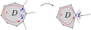
Figure 2: If the boundary word of $D$ has backtracking we may glue up the backtracking and replace it by a disk with shorter boundary word.

4.2 Combinatorial Gauß-Bonnet

Let $\mathcal{D}$ be a van Kampen diagram and let $D$ be a disk of $\mathcal{D}$ (we will also abbreviate this by writing “$D\in\mathcal{D}$”). Recall that every van Kampen diagram has an associated surface $\Sigma_{\mathcal{D}}$ such that the disks in $\mathcal{D}$ decompose $\Sigma_{\mathcal{D}}$ into finitely many polygons glued together along their edges. A vertex $v$ of $\mathcal{D}$ is a vertex of those disks and $\deg(v)$ denotes the degree of $v$, i.e., the number of edges adjacent to $v$ in $\Sigma_{\mathcal{D}}$. Morever, we write $V_{D}$ for the set of all vertices and $E_{D}$ be the set of all edges of $D$.

Definition 4.3 (curvature in a van Kampen diagram).

Let $\mathcal{D}$ be a van Kampen diagram. Then the curvature of disks of $\mathcal{D}$ is define by

$$\kappa(D):=\sum_{v\in V_{D}}\Bigl{(}\frac{1}{\deg(v)}-\frac{1}{2}\Bigr{)}+1.$$

Proposition 4.4 (combinatorial Gauß-Bonnet).

Let $\mathcal{D}$ be a van Kampen diagram on a surface $\Sigma_{\mathcal{D}}$. Then

$$\chi(\Sigma_{\mathcal{D}})=\sum_{D\in\mathcal{D}}\kappa(D).$$

Proof.

Every vertex in $\Sigma_{\mathcal{D}}$ is adjacent to $\deg(v)$ many disks. Thus the total number of vertices in $\Sigma_{\mathcal{D}}$ equals $\sum_{D\in\mathcal{D}}\sum_{v\in V_{D}}\frac{1}{\deg(v)}$. Similarly, $\sum_{D\in\mathcal{D}}\sum_{e\in E_{D}}\frac{1}{2}$ is the total number of edges as every edge is counted twice in the two adjacent disks; and $\sum_{D\in\mathcal{D}}1$ is the total number of disks. Hence,

$$\sum_{D\in\mathcal{D}}\kappa(P)=\#\text{vertices}-\#\text{edges}+\#\text{faces}=\chi(\Sigma_{\mathcal{D}}).\qed$$

If $D$ is a disk in a van Kampen diagram, we may estimate $\kappa(D)$ in terms of the number of vertices of degree at least $3$, so-called branch vertices.

Proposition 4.5.

Let $\mathcal{D}$ be a van Kampen diagram, let $D$ be a disk of $\mathcal{D}$, and let $\beta(D)$ be the number of branch vertices of $D$. Then

$$\kappa(D)\leq\frac{6-\beta(D)}{6}.$$

Proof.

Every vertex in the disk $D$ has degree at least $2$. Thus we compute

$$\kappa(D) =\sum_{v\in V_{D}}\Bigl{(}\frac{1}{\deg(v)}-\frac{1}{2}\Bigr{)}+1$$

$$\leq\sum_{\deg(v)\geq 3}\Bigl{(}\frac{1}{3}-\frac{1}{2}\Bigr{)}+1$$

$$\leq 1-\frac{\beta(D)}{6}=\frac{6-\beta(D)}{6}.\qed$$

4.3 Strong bounds from hyperbolicity

It is generally not known which one-relator groups are hyperbolic [CH20, LW18b]. However, there are two types of elements in $F(S)$ for which hyperbolicity is well-known: proper powers and small cancellation elements. In both cases, we obtain strong lower bounds for the simplicial volume in terms of stable commutator length. The key insight is the following lemma:

Lemma 4.6.

In the situation of Setup 3.1, suppose that there is an $N\geq 7$ such that the infimum in Proposition 4.2 is achieved as the infimum over van Kampen diagrams $\mathcal{D}$ such that $\beta(D)\geq N$ for every $D\in\mathcal{D}$. Then

$$\Bigl{(}1-\frac{6}{N}\Bigr{)}\cdot 4\cdot\operatorname{scl}_{S}(r)\leq\|G_{r}\|.$$

Proof.

Let $\epsilon>0$. Choose a van Kampen diagram $\mathcal{D}$ on a surface $\Sigma_{\mathcal{D}}$ such that $\beta(D)\geq N$ for every $D\in\mathcal{D}$ and such that

$$\|G_{r}\|\geq\frac{-2\cdot\chi^{-}(\Sigma_{\mathcal{D}})}{n(f_{\mathcal{D}},\Sigma_{\mathcal{D}})}-\epsilon.$$

By removing spherical components we may assume that $\chi^{-}(\Sigma_{\mathcal{D}})=\chi(\Sigma_{\mathcal{D}})$. Let $m^{+}$ be the number of positive disks and let $m^{-}$ be the number of negative disks of $\mathcal{D}$. Then the degree is $n(f_{\mathcal{D}},\Sigma_{\mathcal{D}})=m^{+}-m^{-}$ and the total number of disks is $m^{+}+m^{-}$. Using the combinatorial Gauß-Bonnet Theorem (Proposition 4.4) and Proposition 4.5, we see that

$$\chi^{-}(\Sigma_{\mathcal{D}})=\chi(\Sigma_{\mathcal{D}})=\sum_{D\in\mathcal{D}}\kappa(D)\leq\frac{6-N}{6}\cdot(m^{+}+m^{-})$$

and hence

$$\|G_{r}\|+\epsilon\geq\frac{-2\cdot\chi^{-}(\Sigma_{\mathcal{D}})}{n(\Sigma_{\mathcal{D}},f_{\mathcal{D}})}\geq 2\cdot\frac{N-6}{6}\cdot\frac{m^{+}+m^{-}}{m^{+}-m^{-}}.$$

We conclude that

$$\frac{1}{2}\cdot\frac{6}{N-6}\cdot\bigl{(}\|G_{r}\|+\epsilon\bigr{)}\geq\frac{m^{+}+m^{-}}{m^{+}-m^{-}}.$$

Let $\Sigma_{\partial}$ be the surface obtained by removing the $(m^{+}+m^{-})$ disks of $\Sigma_{\mathcal{D}}$. Then $\Sigma_{\partial}$ contracts to the $1$-skeleton of $P_{r}$ via $f_{\partial}$ and every boundary word of $\Sigma_{\partial}$ maps to a word labelled by $r^{\pm}$. Thus $(f_{\partial},\Sigma_{\partial})$ is $\operatorname{scl}$-admissible for $r$; see Definition 2.5. We see that

$$\chi^{-}(\Sigma_{\partial})=\chi^{-}(\Sigma_{\mathcal{D}})-(m^{+}+m^{-})$$

and observe that the $\operatorname{scl}$-degree of $(f_{\partial},\Sigma_{\partial})$ is $(m^{+}-m^{-})$.

This leads to the estimate

$$\operatorname{scl}_{S}(r) \leq \frac{-\chi^{-}(\Sigma_{\partial})}{2\cdot(m^{+}-m^{-})}$$

$$= \frac{-\chi^{-}(\Sigma_{\mathcal{D}})}{2\cdot(m^{+}-m^{-})}+\frac{m^{+}+m^{-}}{2\cdot(m^{+}-m^{-})}$$

$$\leq \frac{1}{4}\cdot\bigl{(}\|G_{r}\|+\epsilon\bigr{)}\cdot\Bigl{(}1+\frac{6}{N-6}\Bigr{)}.$$

As this inequality holds for every $\epsilon$ we conclude that

$$\operatorname{scl}_{S}(r) \leq \frac{1}{4}\cdot\|G_{r}\|\cdot\Bigl{(}1+\frac{6}{N-6}\Bigr{)}$$

and by rearranging terms that

$$\Bigl{(}1-\frac{6}{N}\Bigr{)}\cdot 4\cdot\operatorname{scl}_{S}(r)\leq\|G_{r}\|.\qed$$

We apply Lemma 4.6 to the case of small cancellation elements. Recall that two elements $w,v\in F(S)$ are said to overlap in the word $x$, if $x$ is a prefix of both $w$ and $v$, i.e. if we may write $w=x\cdot w^{\prime}$ and $v=x\cdot v^{\prime}$ as reduced words, for an adequate choice of $w^{\prime},v^{\prime}$. An element $r\in F(S)$ is said to satisfy small cancellation condition $C^{\prime}(1/N)$, if whenever it overlaps in $x$ with a cyclic conjugate of $r$ or $r^{-1}$ that is not equal to $r$, then $|x|\leq\frac{1}{N}\cdot|r|$.

Theorem 4.7 (small cancellation elements).

In the situation of Setup 3.1, if the relator $r\in F(S)^{\prime}\setminus\{e\}$ satisfies the small cancellation condition $C^{\prime}(1/N)$ for some $N\geq 7$, then

$$\Bigl{(}1-\frac{6}{N}\Bigr{)}\cdot 4\cdot\operatorname{scl}_{S}(r)\leq\|G_{r}\|<4\cdot\operatorname{scl}_{S}(r).$$

.

Proof.

If $r$ satisfies the small cancellation condition $C^{\prime}(1/N)$, then for every van Kampen diagram we have that all disks $D$ satisfy $\beta(D)\geq N$. Thus, the first inequality follows from Lemma 4.6. The second inequality holds generally; see Corollary 3.12. ∎

Remark 4.8.

We note that an element $r$ that satisfies small cancellation condition $C^{\prime}(1/N)$ satisfies $\operatorname{scl}_{S}(r)\geq\frac{N-6}{12}$. This can be seen by considering the branch edges, similarly to Proposition 4.5 and computing the Euler characteristic for the corresponding surface with boundary. Thus, using Lemma 4.6, we see that

$$\|G_{r}\|\geq\Bigl{(}1-\frac{6}{N}\Bigr{)}\cdot 4\cdot\frac{N-6}{12}=\frac{N}{3}-1$$

for all $r$ which satisfy small cancellation condition $C^{\prime}(1/N)$ with $N>6$.

On the other hand, we see that for sufficiently large powers, we get a strong connection between stable commutator length and the simplicial volume of one-relator groups.

Theorem 4.9 (proper powers).

In the situation of Setup 3.1, we have for all $N>6$:

$$\Bigl{(}1-\frac{6}{N}\Bigr{)}\cdot 4\cdot\operatorname{scl}(r^{N})\leq\|G_{r^{N}}\|<4\cdot\operatorname{scl}_{S}(r^{N}).$$

In particular, we obtain

$$\lim_{N\to\infty}\frac{\|G_{r^{N}}\|}{N}=4\cdot\operatorname{scl}_{S}(r).$$

Proof.

The second inequality follows from the weak upper bound for simplicial volume (Corollary 3.12). To see the other inequality we will use Lemma 4.6 and show that $\|G_{r^{N}}\|$ may be approximated by van Kampen diagrams $\mathcal{D}$ that satisfy $\beta(D)\geq N$ for all $D\in\mathcal{D}$.

Let $r=\texttt{x}_{0}\cdots\texttt{x}_{n-1}$ with $\texttt{x}_{i}\in S$ be the reduced word representing $r$; we may assume that $r$ is cyclically reduced and not a proper power.

Claim 4.10.

Let $\mathcal{D}$ be a van Kampen diagram on a surface $\Sigma_{\mathcal{D}}$ over $r^{N}$ such that for every van Kampen diagram $\mathcal{D}^{\prime}$ on a surface $\Sigma_{\mathcal{D}^{\prime}}$ over $r^{N}$ with fewer disks than $\mathcal{D}$ we have that

$$\frac{-2\cdot\chi^{-}(\Sigma_{\mathcal{D}})}{n(f_{\mathcal{D}},\Sigma_{\mathcal{D}})}<\frac{-2\cdot\chi^{-}(\Sigma_{\mathcal{D}^{\prime}})}{n(f_{\mathcal{D}^{\prime}},\Sigma_{\mathcal{D}^{\prime}})}.$$ (3)

Let $D\in\mathcal{D}$ be a disk and let $e\subset\partial D$ be a connected subpath of the boundary of $D$ such that $e$ has no branch vertices in the interior.

Then the label of $e$ has word length strictly less than $|r|=n$.

Proof.

Without loss of generality we assume that $D$ is positive, i.e., its boundary is labelled by $r^{N}$. Thus the label $w\in F(S)$ of $e$ is a reduced subword of $r^{N}$ (cyclically written). Assume for a contradiction that $|w|\geq n$. Then, by cyclically relabelling $r$ we may assume that $w=\texttt{x}_{0}\cdots\texttt{x}_{n-1}\tilde{r}$.

Because $e$ has no branch vertices in its interior, there is a disk $D^{\prime}\in\mathcal{D}$ that is adjacent to $e$; let $e^{\prime}$ be the subpath of the boundary of $D^{\prime}$ that corresponds to $e$ in $D$. Then the label of $e^{\prime}$ is $w^{-1}$. We consider two different cases:

• The disk $D^{\prime}$ is positive. Then $w^{-1}$ is a subword of $r^{N}$ (cyclically written) as $e^{\prime}$ is an edge of $D^{\prime}$ and the boundary of $D^{\prime}$ is labelled by the word $r^{N}$. Suppose that the word $w^{-1}$ ends in $\texttt{x}_{i}$. Then we see that $\texttt{x}_{0}^{-1}=\texttt{x}_{i}$. Similarly, we see that $\texttt{x}_{1}^{-1}=\texttt{x}_{i-1}$ and $\texttt{x}_{k}^{-1}=\texttt{x}_{i-k}$ for every $k<i$. If $i$ is even, then this implies that $\texttt{x}_{i/2}^{-1}=\texttt{x}_{i/2}$, which is a contradiction; if $i$ is odd, this implies that $\texttt{x}_{i/2-1/2}^{-1}=\texttt{x}_{i/2+1/2}$, which contradicts that $r$ is a reduced word.

• The disk $D^{\prime}$ is negative. In this case $w^{-1}$ is a subword of $r^{-N}$. By adding degree $2$ vertices to the disks of the van Kampen diagram $\mathcal{D}$, we may assume that every edge is labelled by a single letter in $S^{\pm}$. Suppose that the boundary of $D$ is $e\cdot f$ and that the boundary of $D^{\prime}$ is $f^{\prime}\cdot e^{\prime}$. Here, $a\cdot b$ denotes the concatenation of two paths $a$ and $b$.

  Then $e$ may be written as $e=e_{0}\cdot\cdots e_{n-1}\cdot\tilde{e}$ where $e_{i}$ is labelled by $\texttt{x}_{i}$ for all $i\in\{0,\dots,n-1\}$ and $\tilde{e}$ is labelled by $\tilde{r}$. Similarly, $e^{\prime}$ may be written as $e^{\prime}=\tilde{e}^{\prime}\cdot e^{\prime}_{n-1}\cdots e^{\prime}_{0}$, where $e_{i}^{\prime}$ is labelled by $\texttt{x}_{i}^{-1}$ for all $i\in\{0,\ldots,n-1\}$.

  

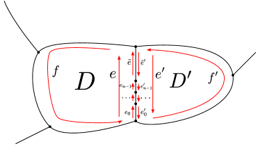
  Figure 3: The disks $D$ and $D^{\prime}$ share the subpaths $e$ and $e^{\prime}$ in $\Sigma_{\mathcal{D}}$.

  The boundary labels of both $D$ and $D^{\prime}$ are $n$-periodic, i.e., after $n$ segments the labels repeat. Thus the first edge of $\tilde{e}$ has to be labelled by $\texttt{x}_{0}$ and the last edge of $\tilde{e}^{\prime}$ has to be labelled by $\texttt{x}_{0}^{-1}$. If we continue comparing the labels of the edges in this way we see that the label for $\tilde{e}$ is inverse to the label for $\tilde{e}^{\prime}$ and that the label for $f$ is inverse to the label for $f^{\prime}$ (see Figure 3).

  Now we may glue both $D$ and $D^{\prime}$ together along the boundaries as in Figure 4.

  

  Figure 4: Gluing up $D$ and $D^{\prime}$.

  This procedure does not change the surface $\Sigma_{\mathcal{D}}$ up to homotopy equivalence. The result is a van Kampen diagram on a surface with the same Euler characteristic. The resulting van Kampen diagram also has the same degree as $\mathcal{D}$ as the degree of both $D$ and $D^{\prime}$ cancelled. This contradicts the minimality of Equation 3.

In both cases we contradicted that the label had word length at least $|r|$. This proves Claim 4.10. ∎

Claim 4.11.

We may approximate $\|G_{r^{N}}\|$ by a sequence of van Kampen diagrams $\mathcal{D}$ that satisfy that $\beta(D)\geq N$ for all $D\in\mathcal{D}$.

Proof.

Let $\epsilon>0$ and let $\Sigma_{\mathcal{D}}$ be a surface with van Kampen diagram $\mathcal{D}$ with the least number of disks such that

$$\|G_{r^{N}}\|\geq\frac{-2\chi^{-}(\Sigma_{\mathcal{D}})}{n(f_{\mathcal{D}},\Sigma_{\mathcal{D}})}-\epsilon.$$

Let $D\in\mathcal{D}$ be a disk in $\mathcal{D}$. Claim 4.10 implies that each connected subpath of the boundary of $D$ without branch vertices has length less than $|r|$. Thus there are at least $|r^{N}|/|r|=N$ such subpaths and branch vertices, i.e., $\beta(D)\geq N$. ∎

Conclusion of the proof of Theorem 4.9. Applying Claim 4.11 to Lemma 4.6, we see that

$$\Bigl{(}1-\frac{6}{N}\Bigr{)}\cdot 4\cdot\operatorname{scl}_{S}(r^{N})\leq\|G_{r^{N}}\|.$$

Using the multiplicativity of stable commutator length we conclude that

$$\lim_{N\to\infty}\frac{\|G_{r^{N}}\|}{N}=4\cdot\operatorname{scl}_{S}(r).\qed$$

5 Random one-relator groups

In this section, we describe the large scale distribution of $\|G_{r}\|$ for random elements $r\in F(S)^{\prime}$. This is an application of Theorem 4.7 and a result by Calegari and Walker on the random distribution of stable commutator lengths in free groups [CW13]. The aim of this section is to show the following result.

Theorem 5.1.

Let $S$ be a finite set, let $\epsilon>0$ and $C>1$. Then, for every random reduced element $r\in F(S)$ of even length $n$, conditioned to lie in the commutator subgroup $F(S)^{\prime}$, we have

$$\biggl{|}\|G_{r}\|\cdot\frac{\log(n)}{n}-\frac{2\cdot\log(2|S|-1)}{3}\biggr{|}\leq\epsilon$$

with probability $1-O(n^{-C})$.

We derive this result by relating the simplicial volume to the stable commutator length of random elements using the small cancellation estimate (Theorem 4.7) and that random elements are small cancellation. The result is then a direct application of the corresponding result for stable commutator length by Calegari and Walker:

Theorem 5.2 (Calegari-Walker [CW13, Theorem 4.1]).

Let $S$ be a finite set, let $\epsilon>0$ and $C>1$. Then, for every random reduced element $r\in F(S)$ of even length $n$, conditioned to lie in the commutator subgroup $F(S)^{\prime}$, we have

$$\left|\operatorname{scl}_{S}(r)\cdot\frac{\log(n)}{n}-\frac{\log(2|S|-1)}{6}\right|\leq\epsilon$$

with probability $1-O(n^{-C})$.

5.1 Random elements of the commutator subgroup

We recall well-known results about random elements of the free group and introduce notation.

Setup 5.3.

Let $S$ be a finite set. We set $k:=|S|$ and let $F:=F(S)$ be the free group over $S$. Furthermore:

• $F_{n}$ denotes the set of all words of length $n$.

• $F^{\prime}_{n}$ denotes the set of all words of length $n$ that lie in the commutator subgroup of $F$. Here, $n$ is supposed to be even.

• $A^{N}_{n}$ denotes the set of all elements (not necessarily cyclically reduced) of length $n$ that do not satisfy the small cancellation condition $C^{\prime}(1/N)$.

In this situation, $|F_{n}|=2k\cdot(2k-1)^{n-1}$. We recall the following Theorem of Sharp, estimating the size of $|F^{\prime}_{n}|$ relative to $|F_{n}|$.

Theorem 5.4 (Sharp [Sha01, Theorem 1][CW13, Theorem 2.1]).

In the situation of Setup 5.3, we have: If $n$ is odd then $F^{\prime}_{n}$ is empty. Moreover, there is an explicit constant $\sigma^{k}$ (which depends only on $k$) such that

$$\lim_{n\to\infty}\left|\sigma^{k}\cdot n^{k/2}\cdot\frac{|F^{\prime}_{n}|}{|F_{n}|}-\frac{2}{(2\pi)^{k/2}}\right|=0,$$

where the limit is taken over all even natural numbers $n$.

We may crudely estimate the exceptional set $|A^{N}_{n}|$ as follows:

Proposition 5.5.

In the situation of Setup 5.3, we have for all natural numbers $n,N\geq 1$:

$$|A^{N}_{n}|\leq 3n^{3}\cdot(2k)^{2}\cdot(2k-1)^{n-\frac{n}{N}}$$

Proof.

Suppose that $w$ does not satisfy the small cancellation condition $C^{\prime}(1/N)$. We consider the following cases:

1. $w\in A^{N}_{n}$ overlaps with a cyclic conjugate of $w^{-1}$ in a piece larger than $n/N$. Then a cyclic conjugate of $w$ may be written as $v=rv_{1}r^{-1}v_{2}$ such that $|r|=\lceil\frac{n}{N}\rceil$ and $|v|=n$ and where there is at most one cancellation either in $v_{1}$ or in $v_{2}$, if $w$ was not cyclically reduced. Here and throughout this section we say that a word has a cancellation if there is a subword $\texttt{x}\cdot\texttt{x}^{-1}$, where x is a letter in the alphabet.

   We will estimate the possible choices for $v$. We have $2k\cdot(2k-1)^{\lceil\frac{n}{N}\rceil-1}$ choices for $r$. If $|v_{1}|=n_{1}$ and $|v_{2}|=n_{2}$, then there are at most $n\cdot 2k\cdot(2k-1)^{n_{1}+n_{2}-1}$ choices for $v_{1}$ and $v_{2}$: For any letter there are $(2k-1)$ choices in order to avoid cancellation with the previous letter, apart from one time where we allow the letter to be an inverse of the previous letter. There are at most $n$ possiblities where such an inverse may occur, and thus we get a total of $n\cdot 2k\cdot(2k-1)^{n_{1}+n_{2}-1}$.

   Thus we estimate that in this case there are a total of

   $$n\cdot(2k)^{2}\cdot(2k-1)^{\lceil\frac{n}{N}\rceil-1}\cdot(2k-1)^{n_{1}+n_{2}-1}$$

   choices for $v=rv_{1}r^{-1}v_{2}$ with $|v_{1}|=n_{1}$ and $|v_{2}|=n_{2}$. We note that $n_{1}+n_{2}+\lceil\frac{n}{N}\rceil=n$, and thus we may crudely estimate that there are

   $$n^{2}\cdot(2k)^{2}\cdot(2k-1)^{\lceil\frac{n}{N}\rceil-1}\cdot(2k-1)^{n-2\cdot\lceil\frac{n}{N}\rceil}$$

   many choices for $v=rv_{1}r^{-1}v_{2}$, such that $r=\lceil\frac{n}{N}\rceil$ and where there is at most one cancellation either in $v_{1}$ or in $v_{2}$. Finally, there are $n$ elements that are cyclically conjugate to such a $v$.

   Thus, an upper bound for the total number of words $w\in A^{n}_{N}$ that overlap with an inverse may be bounded by

   $$n^{3}\cdot(2k)^{2}\cdot(2k-1)^{n-\lceil\frac{n}{N}\rceil}.$$

2. $w\in A^{N}_{n}$ overlaps with a cyclic conjugate of $w$ and $w$ overlaps with itself in a piece $r$ with $|r|=\lceil\frac{n}{N}\rceil$ that does not overlap with itself. Then a cyclic conjugate of $w$ may be written as $v=rv_{1}rv_{2}$ with the conditions on $r$, $v_{1}$ and $v_{2}$ as in case (1.). We may deduce the same bound by replacing $r^{-1}$ by $r$, if appropriate.

   Thus we see that in this case, there are again at most

   $$n^{3}\cdot(2k)^{2}\cdot(2k-1)^{n-\lceil\frac{n}{N}\rceil}.$$

   such elements $w\in A^{N}_{n}$.

3. $w\in A^{N}_{n}$ overlaps with a cyclic conjugate of $w$ and $w$ overlaps with itself in a piece $r$ with $|r|=\lceil\frac{n}{N}\rceil$ that overlaps with itself. Then a cyclic conjugate of $w$ may be written as $v=rv_{1}$ and $v=v_{2}rv^{\prime}_{2}$ for $|r|=\lceil\frac{n}{N}\rceil$, and $|v_{2}|<|r|$. where there is at most one cancellation in $v_{1}$.

   Thus, in particular, we have that $v=rv_{1}^{\prime}$ and $v=v_{2}r$ for $v_{1}^{\prime}$ the prefix of $v_{1}$ such that $|v_{1}^{\prime}|=|v_{2}|$.

   Claim 5.6.

   There are at most $2k\cdot(2k-1)^{M-1}$ elements $v_{2}$, $r$, $v_{1}^{\prime}$, such that $rv_{1}^{\prime}=v_{2}r$, $|v_{2}|=|v_{1}^{\prime}|=M$, $|r|=\lceil\frac{n}{N}\rceil$ and $M<|r|$.

   Proof.

   Indeed, we will see that for any choice of $v_{2}$, the elements $r$ and $v_{1}^{\prime}$ are fully determined: By comparing the first $M$ letters of the equality $rv_{1}^{\prime}=v_{2}r$ we see that the first $|v_{2}|$ letters of $r$ are $v_{2}$. By continuing this way we see that $r$ has to be a prefix of a power of $v_{2}$. We know its length, and thus $r$ is determined. We may recover $v_{1}^{\prime}$ by evaluating $v_{1}^{\prime}=r^{-1}v_{2}r$. There are $2k\cdot(2k-1)^{M-1}$ choices of $v_{2}$, and thus this shows the claim. ∎

   We write $v_{1}=v_{1}^{\prime}\cdot v_{1}^{\prime\prime}$, for $v_{1}$ and $v_{1}^{\prime}$ as above with $|v_{1}^{\prime}|=M$. Note that there is at most one cancellation in $v_{1}$ and thus at most one cancellation in $v_{1}^{\prime\prime}$. Thus, there are at most $n\cdot 2k\cdot(2k-1)^{n-\frac{n}{N}-M-1}$ many choices for $v_{1}^{\prime\prime}$, following the estimate of case (1.) for words that contain exactly one cancellation. Together with Claim 5.6 we see that for $|v_{1}^{\prime}|=M$ there are a total of at most

   $$n\cdot(2k)^{2}\cdot(2k-1)^{n-\frac{n}{N}-2}$$

   choices for such $v$. As $M\leq n$ we see that there are at most a total of

   $$n^{2}\cdot(2k)^{2}\cdot(2k-1)^{n-\frac{n}{N}-2}$$

   choices for $v$ without any condition on $v_{1}^{\prime}$.

   As at most $n$ words in $A^{N}_{n}$ are cyclically conjugate to such a $v$ we may estimate the total of words in $A^{N}_{n}$ with overlap with the same power in itself by

   $$n^{3}\cdot(2k)^{2}\cdot(2k-1)^{n-\frac{n}{N}}.$$

By putting the estimates from the cases (1.), (2.), and (3.) together we deduce that

$$|A^{N}_{n}|\leq 3n^{3}\cdot(2k)^{2}\cdot(2k-1)^{n-\frac{n}{N}}.$$

This finishes the proof of Proposition 5.5. ∎

Corollary 5.7.

In the situation of Setup 5.3, let $q_{n}$ be the probability that a random element of $F^{\prime}_{n}$ does not satisfy the small cancellation condition $C^{\prime}(1/\sqrt{n})$. Then

$$q_{n}=o\bigl{(}(2k-1)^{-\sqrt{n}/2}\bigr{)}.$$

Proof.

Let $B_{n}\subset F_{n}$ be the set of elements that do not satisfy the small cancellation condition $C^{\prime}(1/\sqrt{n})$. By Proposition 5.5 we see that

$$|B_{n}|\leq 3\cdot n^{3}\cdot(2k)^{2}\cdot(2k-1)^{n-\lceil\sqrt{n}\rceil}=3\cdot n^{3}\cdot(2k)\cdot(2k-1)^{1-\lceil\sqrt{n}\rceil}\cdot|F_{n}|.$$

Thus, we may estimate that the probability $q_{n}$ of a random element in $F^{\prime}_{n}$ to also lie in $B_{n}$ to be

$$q_{n}=\frac{|B_{n}|}{|F^{\prime}_{n}|}\leq 3\cdot n^{3}\cdot 2k\cdot(2k-1)^{1-\lceil\sqrt{n}\rceil}\cdot\frac{|F_{n}|}{|F^{\prime}_{n}|}.$$

Using Sharp’s result (Theorem 5.4) we can estimate that $q_{n}=o((2k-1)^{-\sqrt{n}/2})$ as $n\to\infty$. ∎

5.2 Proof of Theorem 5.1

We now give the argument for Theorem 5.1.

Proof.

Let $k:=|S|$. By Theorem 5.2, we see that for every $C>1$, $\epsilon>0$ the probability of a random element in $F^{\prime}_{n}$ to satisfy that

$$\left|\operatorname{scl}(r)\cdot\frac{\log(n)}{n}-\frac{\log(2k-1)}{6}\right|\leq\epsilon$$ (4)

is $1-O(n^{-C})$. By Corollary 5.7, the probability that a random element in $F^{\prime}_{n}$ satisfies the small cancellation condition $C^{\prime}(1/\sqrt{n})$ is $1-o((2k-1)^{-\sqrt{n}/2})$. Thus, the probability that a random element in $F^{\prime}_{n}$ satisfies Equation (4) may be bounded by $1-O(n^{-C})-o((2k-1)^{-\sqrt{n}/2})=1-O(n^{-C})$.

In the following, let $n\geq 49$. Then, Theorem 4.7 implies that

$$4\cdot\operatorname{scl}(r)\cdot\Bigl{(}1-\frac{6}{\sqrt{n}}\Bigr{)}^{-1}\leq\|G_{r}\|\leq 4\cdot\operatorname{scl}(r).$$

Putting things together we see that if $r$ satisfies Equation (4), then

$$\|G_{r}\|\cdot\frac{\log(n)}{n} \leq 4\cdot\operatorname{scl}(r)\cdot\frac{\log(n)}{n}$$

$$\leq\frac{2\log(2k-1)}{3}+4\epsilon$$

and

$$\|G_{r}\|\cdot\frac{\log(n)}{n} \geq 4\cdot\operatorname{scl}(r)\cdot\frac{\log(n)}{n}\cdot\Bigl{(}1-\frac{6}{\sqrt{n}}\Bigr{)}^{-1}$$

$$\geq\frac{2\log(2k-1)}{3}\cdot\Bigl{(}1-\frac{6}{\sqrt{n}}\Bigr{)}^{-1}-4\epsilon\cdot\Bigl{(}1-\frac{6}{\sqrt{n}}\Bigr{)}^{-1}$$

$$\geq\frac{2\log(2k-1)}{3}-2\cdot 4\epsilon. n\geq 36$$ (because )

By relabelling $\epsilon$ and $C$ we obtain that the probability that

$$\left|\|G_{r}\|\cdot\frac{\log(n)}{n}-\frac{2\log(2k-1)}{3}\right|\leq\epsilon$$

may be estimated by $1-O(n^{-C})$. ∎

6 Computational bounds: lallop

In this section we describe an invariant for elements in $F(S)^{\prime}$ called lallop. This invariant will give a lower bound to the simplicial volume of one-relator groups and is computable in polynomial time.

We briefly describe the motivation for the definition of lallop. For this, recall that any element in $F(S)^{\prime}$ may be written up to cyclic conjugation as $r^{M}$, where $r$ is root-free and cyclically reduced and $M\in\mathbb{N}_{>0}$. Throughout this section, we will write $\texttt{lallop}(r^{M})$, to indicate that lallop is evaluated on a power of size $M$, even if the element is root-free, i.e. if $M=1$.

Recall that by Proposition 4.2 we have that

$$\|G_{r^{M}}\|=\inf_{\mathcal{D}\in\Delta(r^{M})}\frac{-2\cdot\chi^{-}(\Sigma_{\mathcal{D}})}{\bigl{|}n(f_{\mathcal{D}},\Sigma_{\mathcal{D}})\bigr{|}},$$

where the infimum ranges over all lallop-admissible van Kampen diagrams. Similar to the algorithm scallop [WC12] that computes stable commutator length of elements in free group, we wish to compute $\|G_{r^{M}}\|$ using a linear programming problem.

Crudely, scallop associates to any $\operatorname{scl}$-admissible surface a vector in a finite dimensional vector space, spanned by the finitely many reasonable configurations around the vertices of $\operatorname{scl}$-admissible surfaces. Then both the Euler characteristic and the degree of the original van Kampen diagram may be computed via linear functions of the associated vector, and thus $\operatorname{scl}$ becomes the solution of a finite dimensional linear programming problem.

When adapting this algorithm for the simplicial volume of one-relator groups one runs into the problem that the Euler characteristic for admissible van Kampen diagrams may not be computed by the information around the vertices alone. However, we remedy this by adding an extra term to the Euler characteristic; see Definition 6.3. This only gives a lower bound of $\|G_{r^{M}}\|$ but allows us to do exact computations. To control this term we will need to restrict to certain van Kampen diagrams, which we call reduced lallop-admissible van Kampen diagrams (see Remark 6.4).

The aim of this section is to show:

Theorem 6.1 (lallop).

Let $S$ be a set and let $r\in F(S)^{\prime}$. Then

1. $\texttt{lallop}(r)\leq\|G_{r}\|$,

2. $\texttt{lallop}(r)\leq 4\cdot\operatorname{scl}_{S}(r)-2$, and

3. there is an algorithm to compute $\texttt{lallop}(r)$ that is polynomial in $|r|$, the word length of $r$. Moreover, $\texttt{lallop}(r)\in\mathbb{Q}$.

We will prove the first two items of Theorem 6.1 in Section 6.2. The proof of the third part will be developed in Sections 6.3 and 6.4.

6.1 lallop

We now define reduced lallop-admissible van Kampen diagrams, which we will use to define lallop in Definition 6.3.

Definition 6.2 (lallop-admissible van Kampen diagram).

Let $r^{M}$ be a cyclically reduced word with root $r=\texttt{x}_{1}\cdots\texttt{x}_{n}\in F(S)^{\prime}\setminus\{e\}$ and $M\in\mathbb{N}_{>0}$. We say that a van Kampen diagram $\mathcal{D}$ to $r$ on a surface $\Sigma_{\mathcal{D}}$ is lallop-admissible to $r^{M}$, if every edge is labelled by a single letter in $S$ such that the counterclockwise label around every disk $D\in\mathcal{D}$ is cyclically labelled by $r^{n\cdot M}$, where $n$ is a non-zero integer $n\in\mathbb{Z}$, called the degree of $D$ and denoted by $n(D)$.

Let $e$ be an oriented edge in the van Kampen diagram. This edge is adjacent to two disks $D$ and $D^{\prime}$, where the edge is in counterclockwise (positive) orientation for one of the disks and in clockwise (negative) orientation in the other. Thus, if the label of the edge $e$ is x, then x labels a subletter of the label of $D$ and a subletter of the inverse of the label of $D^{\prime}$. For $D$ we have a position $i\in\{1,\ldots,n\}$ and a sign $\epsilon\in\{+1,-1\}$ corresponding to the letter $\texttt{x}_{i}$ labelled by that edge in the disk and the sign of the degree of the disk. We will write $i^{\epsilon}$ as a shorthand for the position/sign of the edge at a disk and note that $\texttt{x}_{i}^{\epsilon}=\texttt{x}$. Similarly we have a position and sign for $D^{\prime}$ which we denote by $i^{\prime\epsilon^{\prime}}$ and note that $\texttt{x}_{i^{\prime}}^{\epsilon^{\prime}}=\texttt{x}^{-1}$.

Note that this way, every oriented edge $e$ in the van Kampen diagram has two positions and signs $(i^{\epsilon},i^{\prime\epsilon^{\prime}})$ corresponding to the two disks the edge is adjacent to. In this case, $\texttt{x}_{i}^{\epsilon}=\texttt{x}_{i^{\prime}}^{-\epsilon^{\prime}}$. In analogy to scallop [Cal09a], we call $(i^{\epsilon},i^{\prime\epsilon^{\prime}})$ the rectangle associated to the edge $e$ (Figure 5).

Figure 5: From edges to corresponding rectangles

We say that a lallop-admissible van Kampen diagram is reduced if there are no rectangles $(i^{\epsilon},i^{\prime\epsilon^{\prime}})$ with $i=i^{\prime}$. We denote the set of reduced lallop-admissible van Kampen diagrams to $r^{M}$ by $\operatorname{\Delta_{{\texttt{l}}}}(r^{M})$.

We will see that we may always replace a lallop-admissible van Kampen diagram by a reduced lallop-admissible van Kampen diagram; see Proposition 6.5.

Definition 6.3 (lallop).

Let $s\in F(\mathcal{S})^{\prime}$ be an element in the commutator subgroup of the free group $F(\mathcal{S})$ and let $s$ be conjugate to $r^{M}$ where $r$ is cylically reduced, root-free and $M\in\mathbb{N}_{>0}$. Then, we define

$$\texttt{lallop}(r^{M}):=\inf_{\mathcal{D}\in\operatorname{\Delta_{{\texttt{l}}}}(r^{M})}\frac{-2\chi(\Sigma_{\mathcal{D}})+2\sum_{D\in\mathcal{D}}(1-|n(D)|)}{n(\Sigma_{\mathcal{D}})},$$

where the infimum is taken over all reduced lallop-admissible van Kampen diagrams for $r^{M}$.

As stated in the introduction, the (de)nominator of the terms in the definition of lallop are carefully chosen in such a way that they can be computed using a linear programming problem similar to scallop.

Remark 6.4.

One may wonder why we needed to define reduced lallop-admissible van Kampen diagrams in the first place and didn’t simply take the infimum in Definition 6.3 over all van Kampen diagrams.

To see that this is necessary, note that for every word $r\in F(S)^{\prime}$ and any natural number $N\in\mathbb{N}$ we may glue a disk labelled by $r^{N}$ to a disk labelled by $r^{-N}$ by identifying corresponding letters. Topologically this is a sphere. We may add this sphere to any van Kampen diagram over $r$ to obtain a new van Kampen diagram. While this does not change the total degree of the van Kampen diagram, and only changes the Euler characteristic by $1$, it changes the term $2\sum_{D\in\mathcal{D}}(1-|n(D)|)$ by $2-2\cdot N$. Thus, an infimum as in Definition 6.3 over all lallop-admissible van Kampen diagrams would not exist.

Similarly, if the word we consider is not root-free, say it is of the form $r^{M}$ for some $M\in\mathbb{N}_{\geq 2}$, we may glue up a disk labelled by $r^{N\cdot M}$ with a disk labled by $r^{-N\cdot M}$ by gluing up corresponding letters shifted by $r$. Topologically, this again is a sphere that we may add to any van Kampen diagram.

6.2 From van Kampen diagrams
to reduced lallop-admissible van Kampen diagrams

In this section, we show how an arbitrary van Kampen diagram may be replaced by a reduced lallop-admissible van Kampen diagram:

Proposition 6.5.

Let $r^{M}\in F(S)$ be a cyclically reduced element where $M\geq 1$ and $r$ is root-free. Let $\mathcal{D}$ be a van Kampen diagram for $r^{M}$. Then, there is a reduced lallop-admissible van Kampen diagram $\mathcal{D}^{\prime}$ with the same degree, such that $-\chi(\Sigma_{\mathcal{D}})\geq-\chi(\Sigma_{\mathcal{D}^{\prime}})$.

Moreover, we have for every reduced lallop-admissible van Kampen diagram $\mathcal{D}$ that $\chi(\Sigma_{\mathcal{D}})=\chi^{-}(\Sigma_{\mathcal{D}})$.

Proof.

We may assume that every edge of $\mathcal{D}$ is labelled by some element in $F(S)$ by possibly shrinking the edges that are not labelled by any word. By subdividing the edges, we may further assume that every edge is labelled by a single letter in $S$. We know that every disk is cyclically labelled by a power of $r^{M}$. By recording which letter of $r$ corresponds to which edge, we may construct the rectangles.

Suppose that $\mathcal{D}$ is not reduced. Then there is a rectangle $(i^{\epsilon},i^{\prime\epsilon^{\prime}})$ with $i=i^{\prime}$. Since $\texttt{x}_{i}^{\epsilon}=\texttt{x}_{i^{\prime}}^{-\epsilon^{\prime}}$, we deduce that $\epsilon=-\epsilon^{\prime}$, in other words, the two disks adjacent to this rectangle have opposite signs. We may then cut up the two disks at the edge and glue the boundaries together analogously to Figure 4. This does not change the degree and only increases the Euler characteristic.

We are left to show that $\chi^{-}$ and $\chi$ agree for reduced lallop-admissible van Kampen diagrams. If not, there is a reduced spherical lallop-admissible van Kampen diagram $\mathcal{D}^{S}$ for $r^{M}$, such that $\Sigma_{\mathcal{D}^{S}}$ is a sphere. Note that this would also be a van Kampen diagram for $r$. This would then define a non-trivial spherical map to the presentation complex. However, the presentation complex of root-free words is aspherical by a result of Cockcroft [Coc54]. ∎

Using the last proposition, we may prove items 1 and 2 of Theorem 6.1.

Proof of Theorem 6.1 items 1 and 2.

The fact that $\texttt{lallop}(r)\leq\|G_{r}\|$ is a consequence of the description of $\|G_{r}\|$ in terms of van Kampen diagrams (Proposition 4.2) and that $\chi$ and $\chi^{-}$ agree for reduced lallop-admissible van Kampen diagrams. By Proposition 6.5, we may replace van Kampen diagrams by lallop-admissible van Kampen diagrams.

To see item 2, let $\Sigma$ be an $\operatorname{scl}$-admissible surface to $r^{M}$ with one boundary component. We may assume that we just have one boundary component with positive degree $N$. By gluing in a disk to the boundary we obtain a lallop-admissible van Kampen diagram on a surface $\Sigma^{\prime}$ with $\chi(\Sigma)=\chi(\Sigma^{\prime})-1$. We may estimate

$$\texttt{lallop}(r^{M})\leq\frac{-2\chi(\Sigma^{\prime})+2(1-N)}{N}=\frac{-2\chi(\Sigma)-2N}{N}=4\cdot\frac{-2\chi(\Sigma)}{N}-2$$

Taking the infimum over all $\operatorname{scl}$-admissible surfaces $\Sigma$ to $r^{M}$, shows with the help of the right-hand side that $\texttt{lallop}(r^{M})\leq 4\cdot\operatorname{scl}(r^{M})-2$. ∎

6.3 From reduced lallop-admissible van Kampen diagrams to linear programming

Recall that throughout this section we will write the relator of our one-relator group as $r^{M}$, where $r$ is cyclically reduced and root-free and $M\in\mathbb{N}_{>0}$. Note that any element in the free group may be conjugated to an element that can be written in this way.

Proposition 6.6.

Let $S$ be a set and let $r^{M}\in F(S)^{\prime}\setminus\{e\}$ be cyclically reduced such that $r$ is root-free. Then $\texttt{lallop}(r^{M})$ can be computed via the information around the vertices as follows:

$$\texttt{lallop}(r^{M}) = \inf_{\mathcal{D}\in\operatorname{\Delta_{{\texttt{l}}}}(r^{M})}\frac{\sum_{v\in V_{\mathcal{D}}}\bigl{(}\deg(v)-2\bigr{)}-2\cdot\sum_{D\in\mathcal{D}}|n(D)|}{\sum_{D\in\mathcal{D}}n(D)}$$

Here, we write $V_{\mathcal{D}}$ for the set of vertices of a van Kampen diagram $\mathcal{D}$.

Proof.

Observe that $\sum_{v\in V_{\mathcal{D}}}\bigl{(}\deg(v)-2\bigr{)}$ is equal to $-2\cdot\left(\#\text{vertices}-\#\text{edges}\right)$. Similarly, $2\cdot\sum_{D\in\mathcal{D}}|n(D)|=-2\#\text{faces}+2\sum_{D\in\mathcal{D}}(1-|n(D)|)$. Putting things together we see that

$$\sum_{v\in V_{\mathcal{D}}}\bigl{(}\deg(v)-2\bigr{)}-2\cdot\sum_{D\in\mathcal{D}}|n(D)|=-2\cdot\chi(\Sigma_{\mathcal{D}})+2\cdot\sum_{D\in\mathcal{D}}(1-|n(D)|).$$

Thus, the result follows from the definition of lallop-admissible van Kampen diagrams (Definition 6.2). ∎

A key observation will be that $\texttt{lallop}(r^{M})$ may be computed “locally” by computing the degrees of the vertices in the van Kampen diagram. In contrast, it is impossible to compute the Euler characteristic of the underlying surface in this way because the information of how large the disks are cannot be encoded in the vertices.

In a first step, we will associate to a reduced lallop-admissible van Kampen diagram a vector in an infinite dimensional vector space by encoding the local compatibility conditions around the vertices. We can then compute lallop as an affine function on this vector space. Moreover, we will characterise all vectors that arise in this correspondence (Lemma 6.8).

Let $r^{M}\in F(S)^{\prime}\setminus\{e\}$ be such that $r$ is cyclically reduced and root-free with $M\in\mathbb{N}_{>0}$ and write $r=\texttt{x}_{0}\cdots\texttt{x}_{n-1}$. Let $\mathcal{D}\in\operatorname{\Delta_{{\texttt{l}}}}(r^{M})$ be a reduced lallop-admissible van Kampen diagram.

Recall (Definition 6.2) that for every oriented edge $\bar{e}$ in the reduced lallop-admissible van Kampen diagram $\mathcal{D}$ we associate a pair $(i^{\epsilon},{i^{\prime}}^{\epsilon^{\prime}})$, called rectangle, as follows: The integers $i,i^{\prime}$ correspond to the letters $\texttt{x}_{i}$ and $\texttt{x}_{i^{\prime}}$ that label the sides $e$ and $e^{\prime}$ of $\bar{e}$ and the signs $\epsilon,\epsilon^{\prime}\in\{+1,-1\}$ correspond to the disks adjacent to $\bar{e}$. We denote this rectangle by $\operatorname{R}(\bar{e})$. As $\mathcal{D}$ is reduced we know that $i\not=i^{\prime}$.

By abuse of notation we denote by $\operatorname{R}(r^{M})$ the set

$$\operatorname{R}(r^{M}):=\bigl{\{}(i^{s},i^{\prime s^{\prime}})\bigm{|}i\not=i^{\prime}\in\{0,\ldots,n-1\},\ s,s^{\prime}\in\{+,-\},\ \texttt{x}_{i}^{s}=\texttt{x}_{i^{\prime}}^{-s^{\prime}}\bigr{\}}$$

of all possible rectangles.

Observe that if $\bar{e}^{\prime}$ is the inverse of the oriented edge $\bar{e}$ and if $\operatorname{R}(\bar{e})=(i^{\epsilon},{i^{\prime}}^{\epsilon^{\prime}})$, then $\operatorname{R}(\bar{e}^{\prime})=({i^{\prime}}^{\epsilon^{\prime}},i^{\epsilon})$. This defines an involution $\iota\colon\operatorname{R}(r^{M})\to\operatorname{R}(r^{M})$ on the set of rectangles and we think of $\iota$ as flipping the orientation of the edge (Figure 5).

We now turn to the structure around a vertex: Let $v$ be a vertex of $\mathcal{D}$ and let $\bar{e}_{1},\ldots,\bar{e}_{k}$ be the edges in $\mathcal{D}$ pointing towards $v$ and ordered clockwise around $v$. We associate the tuple

$$\operatorname{V}(v):=\bigl{[}\operatorname{R}(\bar{e}_{1}),\ldots,\operatorname{R}(\bar{e}_{k})\bigr{]}.$$

to $v$. The tuples of rectangles arising in this way are not arbitrary, as they have to be compatible with the labelling of the disks in $\mathcal{D}$. More precisely: Let $\bar{e}_{1}$ have the sides $e_{1}$ and $e^{\prime}_{1}$ with rectangle $\operatorname{R}(\bar{e}_{1})=(i_{1}^{\epsilon_{1}},{i^{\prime}}_{1}^{\epsilon^{\prime}_{1}})$ and let $\bar{e}_{2}$ have the sides $e_{2}$ and $e^{\prime}_{2}$ with rectangle $\operatorname{R}(\bar{e}_{2})=(i_{2}^{\epsilon_{2}},{i^{\prime}}_{2}^{\epsilon^{\prime}_{2}})$; see Figure 6. Then the disk $D$ adjacent to the edges $\bar{e}_{1}$ and $\bar{e}_{2}$ has to have the same sign, i.e., $\epsilon^{\prime}_{1}=\epsilon_{2}$.

Suppose that $\epsilon^{\prime}_{1}=\epsilon_{2}=+$. The labels of the disk $D$ thus read cyclically a positive power of $r$. Hence, if the label of $\bar{e}_{1}$ for $D$ is $\texttt{x}_{i^{\prime}_{1}}$, the label of $\bar{e}_{2}$ is $\texttt{x}_{i_{2}}$ and $i_{2}=i^{\prime}_{1}+1$. Similarly, if the sign of $D$ were negative we would have $i_{2}=i_{1}^{\prime}-1$, where all indices are taken modulo $n$; see Figure 6.

Figure 6: The local structure around a vertex

This motivates the following definition: We say that a rectangle $({i_{1}}^{s_{1}},{i_{1}^{\prime}}^{s_{1}^{\prime}})\in\operatorname{R}(r)$ follows the rectangle $({i_{2}}^{s_{2}},{i_{2}^{\prime}}^{s_{2}^{\prime}})\in\operatorname{R}(r)$ if

• $i^{\prime}_{1}=i_{2}+1$ and $s^{\prime}_{1}=+=s_{2}$, or

• $i^{\prime}_{1}=i_{2}-1$ and $s^{\prime}_{1}=-=s_{2}$.

A tuple $[R_{1},\dots,R_{k}]$ of rectangles $R_{1},\dots,R_{k}\in\operatorname{R}(r)$ is a $k$-pod if $R_{i+1}$ follows $R_{i}$ for all $i\in\{1,\dots,k-1\}$ and $R_{1}$ follows $R_{k}$. We then define

$$\operatorname{V}(r^{M})=\bigl{\{}[R_{1},\ldots,R_{k}]\bigm{|}k\in\mathbb{N}_{\geq 2},\ R_{1},\dots,R_{k}\in\operatorname{R}(r),\ \text{$[R_{1},\dots,R_{k}]$ is a $k$-pod}\bigr{\}}.$$

By construction, if $v$ is a vertex of $\mathcal{D}$, then $\operatorname{V}(v)\in\operatorname{V}(r^{M})$. The set $\operatorname{V}(r^{M})$ is infinite and should be thought of as the set of all possible labels around a vertex in a lallop-admissible van Kampen diagram to $r^{M}$.

We illustrate this by the following example:

Example 6.7.

Let $r=\texttt{a}\texttt{b}\texttt{a}^{-1}\texttt{b}^{-1}$ be the commutator of a and b in $F(\texttt{a},\texttt{b})$. In the above setting, $\texttt{x}_{1}=\texttt{a}$, $\texttt{x}_{2}=\texttt{b}$, $\texttt{x}_{3}=\texttt{a}^{-1}$ and $\texttt{x}_{4}=\texttt{b}^{-1}$. Then

$$\operatorname{R}(r)=\bigl{\{} (1^{+},3^{+}),(3^{+},1^{+}),(1^{-},3^{-}),(3^{-},1^{-}),$$

$$(2^{+},4^{+}),(4^{+},2^{+}),(2^{-},4^{-}),(4^{-},3^{-})\bigr{\}}.$$

Examples of $4$-pods are

$$[(1^{+},3^{+}),(4^{+},2^{+}),(3^{+},1^{+}),(2^{+},4^{+})]\quad\text{or}$$

$$[(1^{-},3^{-}),(2^{-},4^{-}),(3^{-},1^{-}),(4^{-},2^{-})].$$

Let $\mathbb{Z}\operatorname{V}(r^{M})$ be the $\mathbb{Z}$-module freely generated by $\operatorname{V}(r^{M})$. We will now define a map $\Phi\colon\operatorname{\Delta_{{\texttt{l}}}}(r)\to\mathbb{Z}\operatorname{V}(r^{M})$ encoding the local structure of van Kampen diagrams: For a lallop-admissible van Kampen diagram $\mathcal{D}$ on a surface $\Sigma_{\mathcal{D}}$ with vertex set $V_{\mathcal{D}}$, we set

$$\Phi(\mathcal{D}):=\sum_{v\in V_{\mathcal{D}}}\operatorname{V}(v)\in\mathbb{Z}\operatorname{V}(r^{M}).$$

Let $\operatorname{A}(r^{M})\subset\mathbb{Z}V(r^{M})$ be the set of all elements in $\mathbb{N}\operatorname{V}(r^{M})\subset\mathbb{Z}\operatorname{V}(r^{M})$ such that for each rectangle $R\in\operatorname{R}(r^{M})$, the number of occurrences of $R$ coincides with the number of occurrences of the flipped rectangle $\iota(R)$. The set $\operatorname{A}(r^{M})\subset\mathbb{Z}\operatorname{V}(r^{M})$ is defined by a finite set of integral linear equations and inequalities. Furthermore, we will consider the corresponding rational version

$$\operatorname{A}^{\mathbb{Q}}(r^{M})\subset\mathbb{Q}\operatorname{V}(r^{M}),$$

which is defined by the corresponding (in)equalities.

Lemma 6.8.

We have $\Phi(\operatorname{\Delta_{{\texttt{l}}}}(r^{M}))\subset\operatorname{A}(r^{M})$. For every $a\in\operatorname{A}(r^{M})$, there is a van Kampen diagram $\mathcal{D}$ such that $\Phi(\mathcal{D})=2\cdot M\cdot a$.

For the proof we need the following result, originally found in Neumann’s article [Neu01].

Lemma 6.9 ([Neu01, Lemma 3.2]).

Let $\Sigma$ be an oriented surface of positive genus. Let $N\in\mathbb{N}$ be an integer and suppose that for every boundary component of $\Sigma$ there is a collection of degrees summing to $N$. Then there is a connected $N$-fold covering $\Sigma^{\prime}$ of $\Sigma$ with prescribed degrees on the boundary components over each boundary component of $\Sigma$ if and only if the prescribed number of boundary components of the cover has the same parity as $N\cdot\chi(\Sigma)$.

Proof of Lemma 6.8.

By construction, $\Phi(\operatorname{\Delta_{{\texttt{l}}}}(r^{M}))\subset\operatorname{A}(r^{M})$. To prove that for every $a\in\operatorname{A}(r^{M})$ we have that $2\cdot M\cdot a\in\Phi(\operatorname{\Delta_{{\texttt{l}}}}(r^{m}))$, we first assume that $M=1$. In this case, every element of $\operatorname{A}(r)$ gives rise to a lallop-admissible van Kampen diagram over $r$ as follows: Represent pods geometrically by stars. We then choose a matching for the rectangles related by flipping and use this to construct the $1$-skeleton by gluing the corresponding rectangles of the pods with opposite orientations. We now use the ordering of the rectangles in the pods to glue in $2$-disks (whose labels will be non-trivial powers of $r^{M}$ because the rectangles in the pods are following each other). The resulting $2$-dimensional CW-complex is homeomorphic to an orientable closed connected surface [MT01, p. 87] with a lallop-admissible van Kampen diagram $\mathcal{D}$ coming from the labels of the disks. It is easy to see that $\Phi(\mathcal{D})=a$. By taking two copies of $\mathcal{D}$ we conclude the proposition for $M=1$.

Now suppose that $M>1$ and let $a\in\operatorname{A}(r^{M})$. As $\operatorname{A}(r^{M})=\operatorname{A}(r)$, we can first construct a reduced lallop-admissible van-Kampen diagram $\mathcal{D}$ for $\operatorname{A}(r)$. Let $\Sigma_{\mathcal{D}}$ be the associated surface to $\mathcal{D}$ and let $\Sigma^{\partial}_{\mathcal{D}}$ be the surface $\Sigma_{\mathcal{D}}$ with the van Kampen diagrams removed. Thus $\Sigma^{\partial}_{\mathcal{D}}$ is a surface with $|\mathcal{D}|$ many boundary components. We will use the following claim:

Claim 6.10 (coverings of surfaces).

Let $\Sigma$ be a surface with $p$ boundary components and let $M\in\mathbb{N}$. Then there is a covering $\Sigma^{\prime}$ of $\Sigma$, such that each boundary component has degree precisely $M$.

Proof.

We use Lemma 6.9. Suppose that $\Sigma$ has $p$ boundary components. Choose for every boundary of $\Sigma$ two degree $M$ boundaries as in the statement of Lemma 6.9. The resulting map has degree $N=2\cdot M$ and it has $2\cdot p$ boundary components. This is an even number, just as $2\cdot N\cdot\chi(\Sigma)$. Thus, there is a $2\cdot M$-covering $\Sigma^{\prime}$ of $\Sigma$ with the desired property. ∎

Using Claim 4.11, we see that there is a $2\cdot M$-covering ${\Sigma^{\prime}}^{\partial}$ of $\Sigma^{\partial}_{\mathcal{D}}$, where each of the $2\cdot p$ boundaries maps with degree $M$. We may now fill in all the boundaries of ${\Sigma^{\prime}}^{\partial}$ with disks and pull back the labels from $\Sigma_{\mathcal{D}}$. This describes a van Kampen diagram $\mathcal{D}^{\prime}$ on a surface $\Sigma^{\prime}$ with $2|\mathcal{D}|$ disks over $r^{M}$. We see that every vertex of $\mathcal{D}$ corresponds to $2\cdot M$ vertices of $\mathcal{D}^{\prime}$ under the covering and that the labels around the vertices are identical. Thus, $\Phi(\mathcal{D}^{\prime})=2M\cdot a$, as claimed in the proposition. ∎

We will now express the (de)nominators in the computation of $\texttt{lallop}(r^{M})$ in Proposition 6.6 by suitable linear maps on $\mathbb{Z}\operatorname{V}(r^{M})$. For a rectangle $R$, let $s_{1}(R),s_{2}(R)\in\{\pm 1\}$ denote the signs of the first and second component, respectively. We define the following $\mathbb{Z}$-linear maps:

$$\nu\colon\mathbb{Z}\operatorname{V}(r^{M}) \to\mathbb{Q}$$

$$[R_{1},\dots,R_{k}] \mapsto\frac{1}{M\cdot|r|}\cdot\sum_{i=1}^{k}\bigl{(}s_{1}(R_{i})+s_{2}(R_{i})\bigr{)}$$

$$\bar{\nu}\colon\mathbb{Z}\operatorname{V}(r^{M}) \to\mathbb{Q}$$

$$[R_{1},\dots,R_{k}] \mapsto\frac{1}{M\cdot|r|}\cdot 2\cdot k$$

$$\lambda\colon\mathbb{Z}\operatorname{V}(r^{M}) \to\mathbb{Q}$$

$$[R_{1},\dots,R_{k}] \mapsto\frac{1}{2}\cdot(k-2)$$

Lemma 6.11.

If $\mathcal{D}\in\operatorname{\Delta_{{\texttt{l}}}}(r)$, then

$$\nu\bigl{(}\Phi(\mathcal{D})\bigr{)} =\sum_{D\in\mathcal{D}}n(D)$$

$$\bar{\nu}\bigl{(}\Phi(\mathcal{D})\bigr{)} =\sum_{D\in\mathcal{D}}|n(D)|$$

$$\lambda\bigl{(}\Phi(\mathcal{D})\bigr{)} =\frac{1}{2}\cdot\sum_{v\in V_{\mathcal{D}}}\bigl{(}\deg(v)-2\bigr{)}.$$

Proof.

For $\nu$ and $\bar{\nu}$ we only need to note that every occurrence of $r$ will be counted $|r|$ times when counting the two edges of all rectangles (with or without signs). As vertices of degree $k$ in $\mathcal{D}$ are modelled by $k$-pods, the claim for $\lambda$ follows. ∎

Proposition 6.12.

Let $S$ be a set and let $r\in F(S)^{\prime}\setminus\{e\}$. Then $\texttt{lallop}(r)$ is the solution of an infinite linear programming problem that is defined over $\mathbb{Q}$.

Proof.

Using Proposition 6.6 and Lemma 6.8, we see that

$$\texttt{lallop}(r) =\inf_{\mathcal{D}\in\operatorname{\Delta_{{\texttt{l}}}}(r)}\frac{\sum_{v\in V_{\mathcal{D}}}\bigl{(}\deg(v)-2\bigr{)}-2\cdot\sum_{D\in\mathcal{D}}|n(D)|}{\sum_{D\in\mathcal{D}}n(D)}$$

$$=\inf_{a\in\operatorname{A}(r)}2\cdot\frac{\lambda(a)-\bar{\nu}(a)}{\nu(a)}=\inf_{\begin{subarray}{c}a\in\operatorname{A}(r)\\ \nu(a)\geq 1\end{subarray}}2\cdot\frac{\lambda(a)-\bar{\nu}(a)}{\nu(a)}$$

The function on the right-hand side is invariant under scaling. Because the (de)nominator is Lipschitz continuous, we conclude that

$$\texttt{lallop}(r)=\inf_{\begin{subarray}{c}a\in\operatorname{A}^{\mathbb{Q}}(r)\\ \nu^{\mathbb{Q}}(a)\geq 1\end{subarray}}2\cdot\frac{\lambda^{\mathbb{Q}}(a)-\bar{\nu}^{\mathbb{Q}}(a)}{\nu^{\mathbb{Q}}(a)},$$

where $\nu^{\mathbb{Q}}$, $\bar{\nu}^{\mathbb{Q}}$, and $\lambda^{\mathbb{Q}}$ are the rational extensions of the corresponding functions on $\operatorname{A}(r)$. Hence, $\texttt{lallop}(r)$ is the solution of an infinite fractional linear programming problem that is defined over $\mathbb{Q}$. Applying the Charnes-Cooper transformation, shows that $\texttt{lallop}(r)$ is also the solution of a corresponding infinite linear programming problem that is defined over $\mathbb{Q}$. ∎

6.4 Breaking up the pods: A polynomial algorithm

Finally, we reduce the linear programming problem of Proposition 6.12 to a finite linear programming problem (defined over $\mathbb{Q}$), which allows to compute lallop in polynomial time. This will be achieved by “breaking up” the elements in $\operatorname{V}(r^{M})$ into finitely many types of pod-like configurations with two or three edges, which in turn are related by linear equations.

For this we first define abstract pairs of rectangles:

$$\operatorname{RP}(r^{M}):=\{(R_{1},R_{2})\mid R_{1},R_{2}\in\operatorname{R}(r^{M})\}.$$

These rectangles will represent “open” parts in pod fragments. Furthemore, we define the following sets (Figure 7):

• $\operatorname{BP}(r^{M})\subset\operatorname{V}(r^{M})$, the set of all $2$-pods, called bipods,

• $\operatorname{TP}(r^{M})\subset\operatorname{V}(r^{M})$, the set of all $3$-pods, called tripods,

• $\operatorname{OTP}(r^{M}):=\operatorname{OTP}_{1}(r^{M})\sqcup\operatorname{OTP}_{2}(r^{M})$, where

  $$\operatorname{OTP}_{1}(r^{M}) :=\{[R,(R_{1},R_{2})]\mid R,R_{1},R_{2}\in\operatorname{R}(r^{M}),\ \text{$R_{2}$ follows\leavevmode\nobreak\ $R$ and $R$ follows\leavevmode\nobreak\ $R_{1}$}\},$$

  $$\operatorname{OTP}_{2}(r^{M}) :=\{[(R_{2},R_{1}),R]\mid R,R_{1},R_{2}\in\operatorname{R}(r^{M}),\ \text{$R_{2}$ follows\leavevmode\nobreak\ $R$ and $R$ follows\leavevmode\nobreak\ $R_{1}$}\},$$

  the set of open tripods (they are open “between $R_{1}$ and $R_{2}$”),

• $\operatorname{DOTP}(r^{M})=\{\llbracket(R,R_{1}),(R,R_{2})\rrbracket\mid R,R_{1},R_{2}\in\operatorname{R}(r^{M}),\ \text{$R_{2}$ follows $R_{1}$}\}$, the set of doubly open tripods (they are open “between $R$ and $R_{1}$” and “between $R_{2}$ and $R$”).

Figure 7: Breaking up a $k$-pod into (doubly) open tripods

We will now break up pods into these building blocks (Figure 7). Let $\operatorname{B}(r^{M})$ be the free $\mathbb{Z}$-module freely generated by the disjoint union

$$\operatorname{BP}(r^{M})\sqcup\operatorname{TP}(r^{M})\sqcup\operatorname{OTP}(r^{M})\sqcup\operatorname{DOTP}(r^{M})$$

and let $\operatorname{B}^{\mathbb{Q}}(r^{M}):=\mathbb{Q}\otimes_{\mathbb{Z}}\operatorname{B}(r^{M})$. Clearly, $\operatorname{B}^{\mathbb{Q}}(r^{M})$ is finite dimensional. We then consider the $\mathbb{Q}$-linear decomposition map

$$\Phi_{0}\colon\mathbb{Q}\operatorname{V}(r^{M}) \to\operatorname{B}^{\mathbb{Q}}(r^{M})$$

$$[R_{1},\dots,R_{k}] \mapsto\begin{cases}[R_{1},\dots,R_{k}]&\text{if $k\in\{2,3\}$}\\ [R_{1},(R_{k},R_{2})]+\sum_{i=2}^{k-3}\llbracket(R_{k},R_{i}),(R_{k},R_{i+1})\rrbracket+[(R_{k},R_{k-2}),R_{k-1}]&\text{if $k\geq 4$.}\end{cases}$$

If $x\in\operatorname{V}(r^{M})$ and $(R_{1},R_{2})\in\operatorname{RP}(r^{M})$, then the number of occurrences of the pair $(R_{1},R_{2})$ in $\Phi_{0}(x)$ in the first component of (doubly) open tripods coincides with the number of occurrences of $(R_{1},R_{2})$ in the second component. We define the subset $\operatorname{A}_{0}(r^{M})\subset\operatorname{B}(r^{M})$ as the set of all elements such that

1. all coefficients are non-negative and

2. for every $R\in\operatorname{R}(r^{M})$, the number of occurrences of $R$ equals the number of occurrences of $\iota(R)$ and

3. for every $P\in\operatorname{RP}(r^{M})$, the number of occurences of $P$ in the first component equals the number of occurrences of $P$ in the second component.

Furthermore, we consider the corresponding rational version $\operatorname{A}^{\mathbb{Q}}_{0}(r^{M})\subset\operatorname{B}^{\mathbb{Q}}(r^{M})$. By construction, $\Phi_{0}(\operatorname{A}^{\mathbb{Q}}(r^{M}))\subset\operatorname{A}_{0}^{\mathbb{Q}}(r^{M})$. Conversely, by matching up rectangle pairs in the first/second component, we see that $\Phi_{0}(\operatorname{A}^{\mathbb{Q}}(r^{M}))=\operatorname{A}_{0}^{\mathbb{Q}}(r^{M})$.

The functions $\lambda$, $\nu$, and $\bar{\nu}$ can be translated to functions $\lambda_{0},\nu_{0},\bar{\nu}_{0}\colon\operatorname{B}^{\mathbb{Q}}(r^{M})\to\mathbb{Q}$ as follows: On elements of $\operatorname{BP}(r^{M})\sqcup\operatorname{TP}(r^{M})$, we define them as before.

• If $v=[R,(R_{1},R_{2})]\in\operatorname{OTP}_{1}(r^{M})$ or $v=[(R_{2},R_{1}),R]\in\operatorname{OTP}_{2}(r^{M})$, then

  $$\lambda_{0}(v):=\frac{1}{2},\quad\bar{\nu}_{0}(v):=\frac{4}{|r|\cdot M},\quad\nu_{0}(v):=\frac{s_{1}(R_{1})+s_{2}(R)+s_{1}(R)+s_{2}(R_{2})}{|r|\cdot M}.$$

• If $v=\llbracket(R,R_{1}),(R,R_{2})\rrbracket\in\operatorname{DOTP}(r^{M})$, then

  $$\lambda_{0}(v):=\frac{1}{2},\quad\bar{\nu}_{0}(v):=\frac{2}{|r|\cdot M},\quad\nu_{0}(v):=\frac{s_{1}(R_{1})+s_{2}(R_{2})}{|r|\cdot M}.$$

A straightforward computation shows that

$$\lambda_{0}\circ\Phi_{0}=\lambda^{\mathbb{Q}},\quad\bar{\nu}_{0}\circ\Phi_{0}=\bar{\nu}^{\mathbb{Q}},\quad\nu_{0}\circ\Phi_{0}=\nu^{\mathbb{Q}}.$$

We can now complete the proof of Theorem 6.1.3: By Proposition 6.12 and the previous considerations, we have

$$\texttt{lallop}(r^{M})=\inf_{\begin{subarray}{c}a\in\operatorname{A}_{0}^{\mathbb{Q}}(r^{M})\\ \nu_{0}(a)\geq 1\end{subarray}}2\cdot\frac{\lambda_{0}(a)-\bar{\nu}_{0}(a)}{\nu_{0}(a)}.$$

Thus it suffices to solve the (fractional) linear programming problem on $\operatorname{A}_{0}^{\mathbb{Q}}(r^{M})$. The linear cone $\operatorname{A}_{0}^{\mathbb{Q}}(r^{M})$ has only polynomial dimension (namely of order $\mathcal{O}(|r|^{5})$) and via the Charnes-Cooper transform this corresponds to a linear programming problem in the same order of dimension. In particular, $\texttt{lallop}(r^{M})\in\mathbb{Q}$, because everything is defined over $\mathbb{Q}$. There are now several available methods to compute the exact value of a linear programming problem, for example, the algorithm by Karmarkar [Kar84]. Thus, there is an algorithm that determines $\texttt{lallop}(r^{M})$ in polynomial time in $|r|\cdot M$). This finishes the proof of Theorem 6.1.

6.5 Examples

We implemented the algorithm skeleton lallop described in the previous section in MATLAB [HL19] and in Haskell [HL20b]. Thus, we have a polynomial time algorithm to compute lower bounds for $\|G_{r}\|$. Upper bounds, on the other hand, may be computed by finding an explicit van Kampen diagram on a surface for this relator $r$.

We will illustrate this by an example, whose stable commutator length was studied by Calegari [Cal09a, Section 4.3.5][Cal11]: For all $m\in\mathbb{N}_{\geq 2}$, we have

$$\operatorname{scl}_{\{\texttt{a},\texttt{b}\}}(r_{m})=\frac{2m-3}{2m-2},$$

where $r_{m}:=[\texttt{a},\texttt{b}][\texttt{a},\texttt{b}^{-m}]$.

An upper bound for $\|G_{r_{m}}\|$. Calegari [Cal09a, Section 4.3.5] described a van Kampen diagram $\mathcal{D}_{m}$ on a surface $\Sigma_{m}$ of genus $m-1$ with $2m-2$ positive disks that are labelled by the word $r_{m}=[\texttt{a},\texttt{b}][\texttt{a},\texttt{b}^{-m}]$. Thus, using Proposition 4.2, we see that

$$\|G_{r_{m}}\|\leq\frac{-2\cdot\chi(\Sigma_{m})}{n(f_{\mathcal{D}_{m}},\Sigma_{\mathcal{D}_{m}})}=\frac{2m-4}{m-1}=4\cdot\Bigl{(}\operatorname{scl}_{\{\texttt{a},\texttt{b}\}}(r)-\frac{1}{2}\Bigr{)}.$$

We now describe the explicit van Kampen diagram for the case of $r_{3}=\texttt{a}\texttt{b}\texttt{a}^{-1}\texttt{b}^{-1}\texttt{a}\texttt{b}^{-3}\texttt{a}^{-1}\texttt{b}^{-3}$; the resulting surface $\Sigma_{3}$ will have genus $2$ and the van Kampen diagram will consist of four disks. Let us consider Figure 8, where $x_{i}$ is glued to $X_{i}$ for all $i\in\{1,\ldots,13\}$. We may check that the result is a surface of genus $2$. We will label the edges by group elements. For an oriented edge $x$ we will denote the label by $\omega(x)$. If $X$ is the inverse of $x$ then we require that $\omega(X)=\omega(x)^{-1}$. We set:

$$\begin{pmatrix}\omega(x_{1})=\texttt{bA}&\omega(x_{2})=\texttt{b}&\omega(x_{3})=\texttt{bb}&\omega(x_{4})=\texttt{AB}\\ \omega(x_{5})=\texttt{B}&\omega(x_{6})=\texttt{a}&\omega(x_{7})=\texttt{A}&\omega(x_{8})=\texttt{BA}\\ \omega(x_{9})=\texttt{Ab}&\omega(x_{10})=\texttt{Ab}&\omega(x_{11})=\texttt{BA}&\omega(x_{12})=\texttt{bbb}\\ \omega(x_{13})=\texttt{bbb}&&&\end{pmatrix}.$$

We see that this indeed describes an $l^{1}$-admissible van Kampen diagram for $r_{3}$. All of the disks $D_{1},D_{2},D_{3}$ and $D_{4}$ are cyclically labelled by $r$. For example the boundary of $D_{1}$ is (anticlockwise) $x_{10},x_{2},X_{4},X_{5},X_{6},X_{9},X_{13}$, where capitalization of letters corresponds to the inverse of the lower case label. Thus the boundary label is $\texttt{Ab}\cdot\texttt{b}\cdot\texttt{ba}\cdot\texttt{b}\cdot\texttt{A}\cdot\texttt{Ba}\cdot\texttt{BBB}=\texttt{AbbbabABaBBB}$, which is a cyclic conjugate of $r$. The result is a van Kampen diagram on a surface of genus $2$.

Figure 8: An $l^{1}$-admissible van Kampen diagram on a surface $\Sigma_{\mathcal{D}}$ with $\chi(\Sigma_{\mathcal{D}})=-2$ and degree $4$.

A lower bound for $\|G_{r_{m}}\|$. On the other hand, we may compute lower bounds of $\|G_{r_{m}}\|$ using the algorithm described in the previous section [HL19, HL20b]. In this way, we obtained the values $\texttt{lallop}(r_{2})=0$, $\texttt{lallop}(r_{3})=1$, and $\texttt{lallop}(r_{4})=\frac{4}{3}$. We were not able to compute $\texttt{lallop}(r_{i})$ for larger $i$ since the linear programming problem involved in the solution of lallop becomes too large. Using Theorem 6.1 and the upper bounds described above, we deduce that $\|G_{r_{2}}\|=0$, $\|G_{r_{3}}\|=1$ and $\|G_{r_{4}}\|=\frac{4}{3}$.

We summarise these computations in the following proposition:

Proposition 6.13.

Let $m\in\mathbb{N}_{\geq 2}$ and $r_{m}:=[\texttt{a},\texttt{b}][\texttt{a},\texttt{b}^{-m}]$. Then

$$\|G_{r_{m}}\|\leq\frac{2m-4}{m-1}=4\cdot\Bigl{(}\operatorname{scl}_{\{\texttt{a},\texttt{b}\}}(r)-\frac{1}{2}\Bigr{)}.$$

For $m\in\{2,3,4\}$, we have equality, i.e., $\|G_{r_{2}}\|=0,\|G_{r_{3}}\|=1$, and $\|G_{r_{4}}\|=\frac{4}{3}$.

6.6 A counterexample to Question 1.2

Computing $\texttt{lallop}(r)$ is polynomial in the length of $r$, yet it requires lots of time, even for small words. A much more feasable linear programming problem can be built by only considering $2$-, $3$-, and $4$-pods. This gives an upper bound of lallop and drastically speeds up computation. Using such computations, we were able to find a counterexample to the Main Question 1.2:

Example 6.14 (counterexample).

Consider $v=\texttt{aaaabABAbaBAAbAB}$. This element satisfies $\operatorname{scl}_{\{\texttt{a},\texttt{b}\}}(v)=5/8$. However, $\|G_{v}\|=0$. To see this we will show that

$$\operatorname{cl}_{\{\texttt{a},\texttt{b}\}}(v^{-1}+v+v)=1.$$

Indeed, we will compute that

$$\operatorname{cl}_{\{\texttt{a},\texttt{b}\}}(v^{-1}\cdot(t_{1}vt_{1}^{-1})\cdot(t_{2}vt_{2}^{-1}))=1$$

where $t_{1}=\texttt{baBAAAA}$ and $t_{2}=\texttt{baBaabABB}$. In fact, we see that

$$v^{-1}\cdot(t_{1}vt_{1}^{-1})\cdot(t_{2}vt_{2}^{-1})=d\cdot[g,h]\cdot d^{-1}$$

where

$$d = \texttt{baBaabABaBaa},$$

$$g =$$ AAbbaBAAAAAbaBAA, and

$$h = \texttt{bABaaaaaabABBaa}.$$

Nicolaus Heuer
    DPMMS, University of Cambridge, United Kingdom     nh441@cam.ac.uk, https://www.dpmms.cam.ac.uk/ nh441/

Clara Löh
    Fakultät für Mathematik, Universität Regensburg, 93040 Regensburg     clara.loeh@mathematik.uni-r.de, http://www.mathematik.uni-r.de/loeh

References

- [Bav91] Christophe Bavard. Longueur stable des commutateurs. Enseign. Math. (2), 37(1-2):109–150, 1991.
- [BG88] Jean Barge and Étienne Ghys. Surfaces et cohomologie bornée. Invent. Math., 92(3):509–526, 1988.
- [Bro94] Kenneth S. Brown. Cohomology of Groups, volume 87 of Graduate Texts in Mathematics. Springer-Verlag, New York, 1994. Corrected reprint of the 1982 original.
- [Cal09a] Danny Calegari. scl, volume 20 of MSJ Memoirs. Mathematical Society of Japan, Tokyo, 2009.
- [Cal09b] Danny Calegari. Stable commutator length is rational in free groups. J. Amer. Math. Soc., 22(4):941–961, 2009.
- [Cal11] Danny Calegari. scl, sails, and surgery. J. Topol., 4(2):305–326, 2011.
- [CF10] Danny Calegari and Koji Fujiwara. Stable commutator length in word-hyperbolic groups. Groups Geom. Dyn., 4(1):59–90, 2010.
- [CH20] Christopher H. Cashen and Charlotte Hoffmann. Short, highly imprimitive words yield hyperbolic one-relator groups, 2020.
- [CL15] Diarmuid Crowley and Clara Löh. Functorial seminorms on singular homology and (in)flexible manifolds. Algebr. Geom. Topol., 15(3):1453–1499, 2015.
- [Coc54] Wilfred Halliday Cockcroft. On two-dimensional aspherical complexes. Proceedings of the London Mathematical Society, 3(1):375–384, 1954.
- [CSG97] Tullio G. Ceccherini-Silberstein and Rostislav I. Grigorchuk. Amenability and growth of one-relator groups. Enseign. Math. (2), 43(3-4):337–354, 1997.
- [CSS07] John Crisp, Michah Sageev, and Mark Sapir. Surface subgroups of right-angled Artin groups. arXiv e-prints, page arXiv:0707.1144, Jul 2007.
- [CW13] Danny Calegari and Alden Walker. Random rigidity in the free group. Geometry & Topology, 17(3):1707–1744, 2013.
- [CW18] Chris Connell and Shi Wang. Some remarks on the simplicial volume of nonpositively curved manifolds. 2018. arXiv:1801.08597 [math.GT].
- [DH91] Andrew J. Duncan and James Howie. The genus problem for one-relator products of locally indicable groups. Math. Z., 208(2):225–237, 1991.
- [Fri17] Roberto Frigerio. Bounded cohomology of discrete groups, volume 227 of Mathematical Surveys and Monographs. American Mathematical Society, Providence, RI, 2017.
- [Gro82] Michael Gromov. Volume and bounded cohomology. Inst. Hautes Études Sci. Publ. Math., (56):5–99 (1983), 1982.
- [Heu19] Nicolaus Heuer. The full spectrum of scl on recursively presented groups. 2019. arXiv:1909.01309 [math.GR].
- [HL19] Nicolaus Heuer and Clara Löh. lallop. MATLAB program, 2019. https://www.dpmms.cam.ac.uk/ nh441/.
- [HL20a] Nicolaus Heuer and Clara Löh. The spectrum of simplicial volume. Invent. math., 2020. DOI 10.1007/s00222-020-00989-0.
- [HL20b] Nicolaus Heuer and Clara Löh. lallop. Haskell program, 2020. https://gitlab.com/polywuisch/lallop.
- [HL20c] Nicolaus Heuer and Clara Löh. Transcendental simplicial volumes. Annales de l’Institut Fourier, 2020. to appear.
- [Iva85] N. V. Ivanov. Foundations of the theory of bounded cohomology. Zap. Nauchn. Sem. Leningrad. Otdel. Mat. Inst. Steklov. (LOMI), 143:69–109, 177–178, 1985. Studies in topology, V.
- [IY82] Hisao Inoue and Koichi Yano. The Gromov invariant of negatively curved manifolds. Topology, 21(1):83–89, 1982.
- [Kar84] N. Karmarkar. A new polynomial-time algorithm for linear programming. Combinatorica, 4(4):373–395, 1984.
- [KMS60] A. Karrass, W. Magnus, and D. Solitar. Elements of finite order in groups with a single defining relation. Comm. Pure Appl. Math., 13:57–66, 1960.
- [Löh11] Clara Löh. Simplicial volume. Bull. Man. Atl., pages 7–18, 2011.
- [LS01] Roger C. Lyndon and Paul E. Schupp. Combinatorial group theory. Classics in Mathematics. Springer-Verlag, 2001. Reprint of the 1977 edition.
- [LS06] Jean-François Lafont and Benjamin Schmidt. Simplicial volume of closed locally symmetric spaces of non-compact type. Acta Math., 197(1):129–143, 2006.
- [LW18a] Larsen Louder and Henry Wilton. Negative immersions for one-relator groups. arXiv e-prints, page arXiv:1803.02671, Mar 2018.
- [LW18b] Larsen Louder and Henry Wilton. Negative immersions for one-relator groups, 2018.
- [Min01] Igor Mineyev. Straightening and bounded cohomology of hyperbolic groups. Geom. Funct. Anal., 11(4):807–839, 2001.
- [MT01] Bojan Mohar and Carsten Thomassen. Graphs on surfaces. Johns Hopkins Studies in the Mathematical Sciences. Johns Hopkins University Press, 2001.
- [Neu01] Walter D Neumann. Immersed and virtually embedded 1–injective surfaces in graph manifolds. Algebraic & Geometric Topology, 1(1):411–426, 2001.
- [New68] B. B. Newman. Some results on one-relator groups. Bull. Amer. Math. Soc., 74:568–571, 1968.
- [Ols89] Alexander Yu. Olshanskii. Diagrams of homomorphisms of surface groups. Sibirsk. Mat. Zh., 30(6):150–171, 1989.
- [Sha01] Richard Sharp. Local limit theorems for free groups. Mathematische Annalen, 321(4):889–904, 2001.
- [Thu79] William P. Thurston. The geometry and topology of -manifolds. 1979. mimeographed notes.
- [WC12] Alden Walker and Danny Calegari. scallop, computer program. 2012. https://github.com/aldenwalker/scallop.