0cm part[0cm] chapter[1.25cm] []1.25cm  *[0.5pc].  section[1.25cm] []1.25cm [] subsection[1.25cm] []1.25cm  *[.5pc].  [] figure[1em]      *[0.5pc].  [] table[1em]      *[0.5pc].  [] lchapter[0em] []1.25cm  *[.5pc].  lsection[0em] []1.25cm lsubsection[.5em]

Authors



D. Alesini¹, D. Babusci¹, P. Beltrame S.J.², F. Björkeroth¹, F. Bossi¹, P. Ciambrone¹, G. Delle Monache¹, D. Di Gioacchino¹, P. Falferi³, A. Gallo¹, C. Gatti¹, A. Ghigo¹, M. Giannotti⁴ G. Lamanna⁵, C. Ligi¹, G. Maccarrone¹, A. Mirizzi⁶, D. Montanino⁷, D. Moricciani¹, A. Mostacci⁷, M. Mück⁸, E. Nardi¹, F. Nguyen⁹, L. Pellegrino¹, A. Rettaroli^1,10, R. Ricci¹, L. Sabbatini¹, S. Tocci¹, L. Visinelli<sup>11


1</sup> INFN - Laboratori Nazionali di Frascati, via E. Fermi 40, 00044 Frascati, Italy.
² Specola Vaticana, V-00120 Vatican City, Vatican City State and Vatican Observatory Research Group Steward Observatory, The University Of Arizona, 933 North Cherry Avenue, Tucson, Arizona 85721, USA
³ Istituto di Fotonica e Nanotecnologie, CNR—Fondazione Bruno Kessler, and INFN-TIFPA,
I-38123 Povo (Trento), Italy.
⁴ Physical Sciences, Barry University, 11300 NE 2nd Ave., Miami Shores, FL 33161, USA.
⁵ Università di Pisa and INFN Pisa, Italy.
⁶ Dipartimento Interateneo di Fisica “Michelangelo Merlin”, Università degli Studi di Bari, Bari, Italy.
⁷ Università del Salento and INFN Lecce, Italy.
⁸ ez SQUID Mess- und Analysegeräte, D-35764 Sinn, Germany.
⁹ ENEA - Centro Ricerche Frascati, via E. Fermi 45, 00044 Frascati, Italy
¹⁰ Università “Roma3" e INFN Roma3, Italy.
¹¹ Gravitation Astroparticle Physics Amsterdam (GRAPPA), Institute for Theoretical Physics Amsterdam and Delta Institute for Theoretical Physics, University of Amsterdam, Science Park 904, 1098 XH Amsterdam, The Netherlands.

The axion, a pseudoscalar particle originally introduced by Peccei, Quinn [1, 2], Weinberg [3], and Wilczek [4] to solve the “strong CP problem”, is a well motivated dark-matter (DM) candidate with a mass lying in a broad range from peV to few meV [5]. The last decade witnessed an increasing interest in axions and axion-like particles with many theoretical works published and many new experimental proposals [6] that started a real race towards their discovery. Driven by this new challenge and stimulated by the availability, at the Laboratori Nazionali di Frascati (LNF), of large superconducting magnets previously used for particle detectors [7, 8] at the DAFNE collider, we proposed to build a large haloscope [9] to observe galactic axions in the mass window between 0.2 and 1 $\mu$eV [10].

This paper is the Conceptual Design Report (CDR) of the KLASH (KLoe magnet for Axion SearcH) experiment, designed having in mind the performance and dimensions of the KLOE magnet, a large volume superconducting magnet with a moderate magnetic field of 0.6 T. In the first part of this Report we discuss the physics case of KLASH, the theoretical motivation for an axion in the mass window $0.1\div 1\,\mu$eV based on a review of standard and non-standard axion-cosmology (Sec. 1), and the physics reach of the KLASH experiment (Sec. 2), including both the sensitivity to QCD axions and to Dark-Photon DM. The sensitivity plots are based on the detector performance discussed in the second part of the CDR. Here, we summarize the results obtained with calculations and simulations of several aspects of the experiment: the mechanical construction of cryostat and cavity based on the study commissioned to the mechanical engineers of the Fantini-Sud company [11] (Sec. 3); the cryogenics plant (Sec. 4); the RF cavity design and tuning based on detailed simulations with code Ansys-HFSS (Sec. 5); the signal amplification, in particular the first stage based on a Microstrip SQUID Amplifier (Sec. 6).

Finally, in Sec. 7, mainly based on the experience of existing experiments [12, 13, 14], we discuss the data taking, analysis procedure and computing requirements.

The main conclusion we draw from this report is the possibility to build and put in operation at LNF in 2-3 years a large haloscope with the sensitivity to KSVZ axions in the low mass range between 0.2 and 1$\mu$eV in a region complementary to that of other experiments with a cost of about 3 M€. Timeline and cost are competitive with respect to other proposals in the same mass region [15, 16] thanks to the availability of most of the infrastructure, in particular the superconducting magnet and the cryogenics plant.

During the writing of this CDR, in July 2019, we were informed about the decision of INFN management to devote the KLOE magnet to the DUNE experiment at Fermilab. The KLOE magnet has always been the preferred choice for several reasons: it was in operation until 2018; its mechanical structure is able to support the several-tons weight of the cryostat and cavity; it is placed in the KLOE assembly-hall that can be used as the experimental area of KLASH. However, another option is given by the FINUDA magnet. The are few aspects to be explored (mechanical strength, move to experimental area, put in operation after more than 10 years), but it has a higher nominal field of 1.1 T in a large volume with an inner radius 1385 mm and length 3800 mm. A preliminary estimate of sensitivity to axions of FLASH, the haloscope built with the FINUDA magnet, gives results similar to those obtained for KLASH. This option will be eventually investigated in another document.

Acknowledgements

L.V. thanks for the hospitality at Istituto Nazionale di Fisica Nucleare (INFN), Laboratori Nazionali di Frascati (LNF). L.V. acknowledges support by the Vetenskapsrådet (Swedish Research Council) through contract No. 638-2013-8993 and the Oskar Klein Centre for Cosmoparticle Physics. This work is part of the research program "The Hidden Universe of Weakly Interacting Particles" with project number 680.92.18.03 (NWO Vrije Programma), which is (partly) financed by the Dutch Research Council (NWO).

Contents

1. I Physics Case
   1. 1 The KLASH Physics Case
      1. 1.1 Brief review on axion cosmology
         1. 1.1.1 The temperature dependence of the QCD axion mass
         2. 1.1.2 Production of cold axions in the early universe
         3. 1.1.3 Axion cosmology and the inferred dark matter axion mass
      2. 1.2 Dark matter axion mass in the range of KLASH
         1. 1.2.1 I.   Initial misalignment angle
         2. 1.2.2 II.  Modified cosmological evolution
         3. 1.2.3 III.  Extended QCD axion models
   2. 2 Physics Reach
      1. 2.1 Summary of KLASH Haloscope
      2. 2.2 The KLASH Sensitivity
      3. 2.3 Dark Photons sensitivity
2. II Conceptual Design
   1. 3 Mechanical Design
      1. 3.1 Cryostat general description
      2. 3.2 Vacuum vessel
      3. 3.3 Cryostat support
      4. 3.4 Cavity
      5. 3.5 Tuning system
      6. 3.6 Shield
      7. 3.7 Mounting sequence
      8. 3.8 Preliminary structural simulations
   2. 4 Cryogenics
      1. 4.1 The cryogenic plant
      2. 4.2 The cryogenics layout
      3. 4.3 The KLASH service turret
      4. 4.4 The KLASH cryostat cryogenics
      5. 4.5 The KLASH cryogenics diagnostic
   3. 5 RF
      1. 5.1 Cavity Design and Tuning
   4. 6 Signal Amplification and Acquisition
      1. 6.1 SQUID
         1. 6.1.1 B Field Shielding
      2. 6.2 Secondary Amplification
   5. 7 Analysis
      1. 7.1 Introduction
      2. 7.2 Spectra Combination and Analysis
         1. 7.2.1 Cut on raw data and problematic bin
         2. 7.2.2 Normalization and baseline subtraction
         3. 7.2.3 Candidates and Rescan
         4. 7.2.4 Limits
      3. 7.3 Computing
3. III Bibliography

Part I Physics Case

Chapter 1 The KLASH Physics Case

1.1 Brief review on axion cosmology

The “invisible” QCD axion [3, 4] is a light Goldstone boson arising within the solution to the strong CP problem proposed by Peccei and Quinn [1, 2], and a possible dark matter candidate [17, 18, 19]. In the standard cosmological scenario, refined cosmological simulations yield a narrow range in which the QCD axion would be the CDM particle, with an axion mass in the range $\displaystyle m_{A}\approx(10-100)\,\mu{\rm eV}$, as recently proven by refined cosmological simulations [20, 21, 22, 23]. Along with the QCD axion, a set of particles which share the same phenomenology would arise from string compactification and form the so-called “axiverse” [24, 25, 26, 27, 28, 29, 30, 31, 32, 33, 34]. These possibilities have been proven interesting for a number of experiments that are planned to explored the parameter space of the QCD axion and other axion-like particles away from the preferred region [35, 36, 37], as discussed in depth in various reviews on the subject [38, 39, 40, 41, 42, 43, 44, 45, 6].

1.1.1 The temperature dependence of the QCD axion mass

The QCD axion mass originates from non-perturbative effects during the QCD phase transition. At zero temperature, the axion gets a mass $\displaystyle m_{0}$ from mixing with the neutral pion [3],

$$m_{0}=\frac{\Lambda^{2}}{f_{A}}=\frac{\sqrt{z}}{1+z}\,\frac{m_{\pi}f_{\pi}}{f_{A}},$$ (1.1)

where $\displaystyle z=m_{u}/m_{d}$ is the ratio of the masses of the up and down quarks, $\displaystyle m_{\pi}$ and $\displaystyle f_{\pi}$ are respectively the mass and the decay constant of the pion, and $\displaystyle f_{A}$ is the QCD axion energy scale. Since the mass of the axion is tied to the underlying QCD theory, the energy scale $\displaystyle\Lambda$ is related to the QCD scale $\displaystyle\Lambda_{\rm QCD}$. Using $\displaystyle z=0.48(5)$, $\displaystyle m_{\pi}=132\,$MeV, and $\displaystyle f_{\pi}=92.3\,$MeV gives $\displaystyle\Lambda=75.5\,$MeV [3]. This value has been confirmed by dedicated lattice simulations [46, 47, 48, 49], in which the goal is to compute the QCD topological susceptibility $\displaystyle\chi(T)$ normalised so that at zero temperature $\displaystyle\chi(0)=\Lambda^{4}$. We show the topological susceptibility around the QCD phase transition in Fig. 1.1, which contains the results obtained by the lattice simulation in Ref. [48].

At temperatures higher than that of the QCD phase transition, the effects of instantons become severely suppressed. This reflects onto the value of the axion mass, whose dependence on the temperature is fixed in terms of the QCD topological susceptibility as $\displaystyle\chi(T)\equiv f_{A}^{2}m_{A}^{2}(T)$. The axion mass decreases quickly with an increasing value of the temperature of the plasma above the confinement temperature $\displaystyle T_{C}$ [50, 51]. Here, we parametrise this dependence as [50]

$$m_{A}(T)=m_{0}\left(\frac{T_{C}}{T}\right)^{\gamma},$$ (1.2)

where $\displaystyle m_{0}$ is the mass of the axion at zero temperature, $\displaystyle T_{C}$ is a confinement temperature, and the exponent depends on temperature as

$$\gamma=\begin{cases}0&\hbox{for $\displaystyle T\leq T_{C}$},\\ \gamma_{\infty},&\hbox{for $\displaystyle T\geq T_{C}$}.\end{cases}$$ (1.3)

The exponent $\displaystyle\gamma_{\infty}$ has been obtained with various techniques, as for example from lattice computations or by using the dilute instanton gas approximation [50, 52, 53], or relying on the interacting instanton liquid model [54]. In the QCD axion theory, the mass $\displaystyle m_{0}$ depends on the axion energy scale $\displaystyle f_{A}$, which represents the energy at which the Peccei-Quinn U(1) symmetry breaks, through Eq. (1.1), $\displaystyle m_{0}f_{A}=\Lambda^{2}$. Here, we choose to present results in terms of the axion mass $\displaystyle m_{0}$, in place of the energy scale $\displaystyle f_{A}$, and we assume the values $\displaystyle T_{C}=140{\rm\leavevmode\nobreak\ MeV}$ and $\displaystyle\gamma_{\infty}=4$, in line with the numerical results in Ref. [48].

Figure 1.1: The topological susceptibility $\displaystyle\chi(T)$ as a function of temperature. The width of the line represents the combined statistical and systematic errors. The insert shows the behavior around the transition temperature. For additional details see Ref. [48].

1.1.2 Production of cold axions in the early universe

Cold axions are produced in the early universe through various mechanisms, which include the vacuum realignment mechanism (VRM), the decay of topological defects, or the decay from a parent particle. In the VRM, the present energy density stored in the axion field $\displaystyle\phi(x)$ from the coherent oscillations of the field can be obtained by solving the equation of motion in an expanding universe

$$\ddot{\phi}+3H\dot{\phi}+\frac{dV(\phi)}{d\phi}=0,$$ (1.4)

where a dot means a derivative with respect to cosmic time $\displaystyle t$. The axion potential in Eq. (1.4) has been computed in the next-to-leading order as [55, 56]

$$V(\phi)=\frac{\Lambda^{4}}{c_{z}}\left(1-\sqrt{1-4c_{z}\sin^{2}(\phi/2f_{A})}\right),$$ (1.5)

where we introduced $\displaystyle c_{z}\approx z/(1+z)^{2}\approx 0.22$.

The axion potential becomes a relevant term in the equation of motion at the temperature $\displaystyle T_{\rm osc}$ when the universe has sufficiently cooled so that the axion mass is of the same order as the Hubble rate

$$m_{A}(T_{\rm osc})\approx 3H(T_{\rm osc}),$$ (1.6)

where $\displaystyle H(T)$ is the Hubble expansion rate for the temperature of the plasma $\displaystyle T$. We assume that the coherent oscillations in the axion field take place in a radiation-dominated universe, for which the expansion rate is given by

$$H(T)=\sqrt{\frac{4\pi^{3}}{45}\,g_{*}(T)}\,\frac{T^{2}}{M_{\rm P}},$$ (1.7)

where $\displaystyle M_{\rm P}\approx 1.221\times 10^{19}\,$GeV is the Planck mass and $\displaystyle g_{*}(T)$ is the number of relativistic degrees of freedom at temperature $\displaystyle T$, corresponding to the number of relativistic species in thermal equilibrium at $\displaystyle T$ weighted with a statistical factor (1 for bosons, 7/8 for fermions). The initial conditions for solving the equation of motion are the initial value $\displaystyle\theta_{i}$ of the misalignment of the axion angular variable $\displaystyle\theta=\phi(x)/f_{A}$, which is drawn randomly from a uniform distribution in the interval $\displaystyle\left[-\pi,\pi\right]$, and a vanishing initial value for the velocity $\displaystyle\dot{\phi}(x)$.

Inserting the expressions in Eqs. (1.2) and (1.7) into Eq. (1.6), we obtain the value

$$T_{\rm osc}=T_{C}\,\left[\sqrt{\frac{5}{4\pi^{3}\,g_{*}(T_{\rm osc})}}\frac{m_{0}M_{\rm P}}{T_{C}^{2}}\right]^{\frac{1}{2+\gamma}}\approx 700{\rm\,MeV}\,\left(\frac{m_{0}}{1{\rm\,\mu eV}}\right)^{1/6},$$ (1.8)

where in the numerical estimate we have set $\displaystyle\gamma=4$ and $\displaystyle g_{*}(T_{\rm osc})=61.75$, which is the number of relativistic degrees of freedom in the Standard Model at a temperature of order GeV. The number density of axions at the onset of oscillations is then

$$n_{A}(T_{\rm osc})=\frac{b}{2}m_{A}(T_{\rm osc})\,f_{A}^{2}\,\langle\theta_{i}^{2}\rangle,$$ (1.9)

where $\displaystyle b$ is a factor of order one [52] that captures the uncertainties derived from using the approximation in Eq. (1.6) instead of numerically solving Eq. (1.4), and $\displaystyle\langle\theta_{i}^{2}\rangle$ is the average of the square of the initial value of the initial misalignment angle $\displaystyle\theta_{i}$ over the observable universe (see the discussion in Sec. 1.1.3 below).

The present number density of axions is obtained by assuming that their number in a comoving volume is constant,

$$n_{A}(T_{0})=n_{A}(T_{\rm osc})\,\left(\frac{a(T_{\rm osc})}{a(T_{0})}\right)^{3},$$ (1.10)

where $\displaystyle T_{0}$ is the present CMB temperature. The ratio of the two comoving volumes at temperatures $\displaystyle T_{\rm osc}$ and $\displaystyle T_{0}$ is given in the standard cosmological model by assuming entropy conservation in the same comoving volume, that is

$$g_{S}(T_{\rm osc})\,a^{3}(T_{\rm osc})\,T_{\rm osc}^{3}=g_{S}(T_{0})\,a^{3}(T_{0})\,T_{0}^{3},$$ (1.11)

where $\displaystyle g_{S}(T)T^{3}$ is the entropy density, with $\displaystyle g_{S}(T)$ the number of entropy degrees of freedom at temperature $\displaystyle T$ [57]. The present energy density of axions $\displaystyle\rho_{A}^{\rm mis}=m_{0}n_{A}(T_{0})$ obtained from the VRM results in

$$\displaystyle\rho_{A}^{\rm mis} \displaystyle= \displaystyle\frac{b}{2}\,m_{0}^{2}\,f_{A}^{2}\,\left(\frac{T_{\rm osc}}{T_{C}}\right)^{-\gamma}\,\left(\frac{a(T_{\rm osc})}{a(T_{0})}\right)^{3}\,\langle\theta_{i}^{2}\rangle=\frac{b}{2}\,\Lambda^{4}\,\frac{g_{S}(T_{0})}{g_{S}(T_{\rm osc})}\,\left(\frac{T_{0}}{T_{C}}\right)^{3}\,\left(\frac{T_{C}}{T_{\rm osc}}\right)^{3+\gamma}\,\langle\theta_{i}^{2}\rangle$$ (1.12)

$$\displaystyle= \displaystyle b\,\mathrm{bar}{\rho}\,\left(\frac{m_{0}}{M_{\rm P}}\right)^{-\frac{3+\gamma}{2+\gamma}}\,\langle\theta_{i}^{2}\rangle=6.1\times 10^{-47}{\rm\,GeV^{4}}\,b\,\left(\frac{m_{0}}{1{\rm\,\mu eV}}\right)^{-7/6}\,\langle\theta_{i}^{2}\rangle.$$

In the last expression, we have introduced the quantity

$$\mathrm{bar}{\rho}=\frac{\Lambda^{4}}{2}\,\frac{g_{S}(T_{0})}{g_{S}(T_{\rm osc})}\,\left(\frac{T_{0}}{T_{C}}\right)^{3}\,\left[\sqrt{\frac{5}{4\pi^{3}\,g_{*}(T_{\rm osc})}}\frac{M_{\rm P}^{2}}{T_{C}^{2}}\right]^{-\frac{3+\gamma}{2+\gamma}}=1.05\times 10^{-50}{\rm\,eV^{4}},$$ (1.13)

where we have set $\displaystyle g_{S}(T_{0})=3.91$, $\displaystyle g_{S}(T_{\rm osc})=g_{*}(T_{\rm osc})=61.75$, and $\displaystyle T_{0}=236{\rm\,\mu eV}$. This computation only relies on the contribution to the energy density in axions from the energy density stored in the coherent oscillations of the field. Additional contributions come from the low-energy spectra of axions radiated from the decay of various topological defects, like axionic strings and domain walls [58, 59, 60], as described in Sec. 1.1.3 below. We account for this contribution by introducing a factor $\displaystyle\alpha_{\rm td}$ multiplying the energy density from the VRM, so that the total axion energy density today is written as $\displaystyle\rho_{A}^{\rm tot}=\alpha_{\rm td}\rho_{A}^{\rm mis}$. The requirement that axions account for the full amount of dark matter then reads

$$\rho_{A}^{\rm tot}=\rho_{\rm CDM}=\Omega_{\rm CDM}\frac{3H_{0}^{2}M_{\rm P}^{2}}{8\pi}\approx 9.71\times 10^{-48}{\rm\,GeV^{4}}.$$ (1.14)

The numerical estimate corresponds to the value of the dark matter energy density in units of the present critical energy density $\displaystyle\Omega_{\rm CDM}h^{2}\approx 0.12$. The contribution from both topological defects and from the VRM to compute the energy density in cold axions $\displaystyle\rho_{A}^{\rm tot}$ has been the subject of various numerical simulations [61, 62, 63, 64, 65, 66, 67, 20, 21, 22, 23].

1.1.3 Axion cosmology and the inferred dark matter axion mass

The actual value of $\displaystyle\langle\theta_{i}^{2}\rangle$ strongly depends on the cosmological history of the axion. We first define two conditions:

• The Peccei-Quinn symmetry is spontaneously broken during inflation;

• The Peccei-Quinn symmetry is never restored after its spontaneous breaking occurs.

Condition a) is realised whenever the Peccei-Quinn scale is larger than the Hubble rate at the end of inflation, $\displaystyle f_{A}>H_{I}$, while condition b) is realised whenever the Peccei-Quinn scale is larger than the maximum temperature of the post-inflationary universe $\displaystyle T_{\rm MAX}$, which is generally higher than the reheating temperature $\displaystyle T_{\rm RH}$ [68]. Broadly speaking, one of these two possible scenarios occurs:

Scenario I

If both a) and b) are satisfied, inflation selects one patch of the universe within which the spontaneous breaking of the Peccei-Quinn symmetry leads to a homogeneous value of the initial misalignment angle $\displaystyle\theta_{i}$. This is the so-called pre-inflationary scenario, in which the distribution of $\displaystyle\theta_{i}$ has the second moment $\displaystyle\langle\theta_{i}^{2}\rangle=\theta_{i}^{2}+\sigma_{\theta}^{2}$, where $\displaystyle\sigma_{\theta}$ is the standard deviation of the distribution of the angle centered around $\displaystyle\theta_{i}$. In this scenario, topological defects are inflated away and do not contribute to the axion energy density. Namely we can set $\displaystyle\alpha_{\rm td}=1$ and $\displaystyle\rho_{A}^{\rm tot}=\rho_{A}^{\rm mis}$. Inserting these conditions into Eqs. (1.12) and (1.14) gives

$$m_{0}=M_{\rm P}\,\left[b\frac{\mathrm{bar}{\rho}}{\rho_{\rm CDM}}\,\left(\theta_{i}^{2}+\sigma_{\theta}^{2}\right)\right]^{\frac{2+\gamma}{3+\gamma}}\approx 5{\rm\,\mu eV}\,\theta_{i}^{12/7}.$$ (1.15)

For the numerical estimate, we have set $\displaystyle b=1$ and $\displaystyle\gamma=4$, and we have assumed that the standard deviation of the distribution in the initial misalignment angle is much smaller than the value realised, which is justified whenever $\displaystyle H_{I}\ll\theta_{i}\,f_{A}$. As we will detail in the next section, within this scenario, KLASH would be able to test the QCD axion for values of the initial misalignment angle within the range $\displaystyle|\theta_{i}|\in\left(0.2-0.4\right)$ which, although it covers only a few percent of the full range, it is outside the reach of all other axion search experiments proposed so far.

Figure 1.2: Sensitivities of various haloscope experiments. The region hatched in black represents the canonical dark matter axion window in post-inflationary scenarios. The region hatched in white represents the additional mass range for axion dark matter which becomes viable in the various theoretical scenarios discussed in the text.

Scenario II

If at least one of the conditions a) or b) is violated, the Peccei-Quinn symmetry breaks with different values of $\displaystyle\theta_{i}$ taking different values in patches that are initially out of causal contact, but that today populate the volume enclosed by our Hubble horizon. In this scenario, which is generally referred to as post-inflationary scenario, $\displaystyle\langle\theta_{i}^{2}\rangle$ is the average of the initial misalignment angle squared over the circle, assuming that $\displaystyle\theta_{i}$ is drawn from a uniform distribution. For a quadratic potential one has $\displaystyle\langle\theta_{i}^{2}\rangle=\pi^{2}/3$, however, in the periodic potential that defines the QCD axion, this result is modified due to the presence of non-harmonic terms [52]. In particular, for a cosine potential we have $\displaystyle\langle\theta_{i}^{2}\rangle\approx(2.15)^{2}$ [56]. We will use this value in our computations.

In this scenario, topological defects form after inflation and remain within the horizon. Hence they contribute to the present energy density ($\displaystyle\alpha_{\rm td}\neq 1$). The detailed mechanism of cold axion production from topological defects has yet to be assessed with sufficient confidence and precision, and an agreement is yet to be achieved in the community. Available estimates differ by as much as one order of magnitude, spanning a range $\displaystyle\alpha_{\rm td}=\left(0.5-10\right)$ (see Eq. (1.12)). Computing the mass of the dark matter axion from Eq. (1.14) in this scenario gives

$$m_{0}=M_{\rm P}\,\left(b\,\frac{\alpha_{\rm td}\,\mathrm{bar}{\rho}}{\rho_{\rm CDM}}\,\langle\theta_{i}^{2}\rangle\right)^{\frac{2+\gamma}{3+\gamma}}\approx\left(5-50\right){\rm\,\mu eV},$$ (1.16)

where, as in the previous scenario, we have taken $\displaystyle b=1$ and $\displaystyle\gamma=4$, and we have set $\displaystyle\langle\theta_{i}^{2}\rangle\approx(2.15)^{2}$ and $\displaystyle\alpha_{\rm td}$ spanning the range given above. Therefore, as is depicted in Fig. 1.2, in this scenario the possible values of the axion mass hinted by cosmological considerations remain well above the mass region accessible to KLASH.

1.2 Dark matter axion mass in the range of KLASH

We have seen in the previous section that assuming a standard cosmological evolution, only in the case of pre-inflationary scenarios are canonical axion models within the reach of KLASH sensitivity, and the region of the initial misalignment angle for which this happens is rather restricted. At the root of this conclusion lies the axion equation of motion Eq. (1.4) which depends on three crucial ingredients: (I) the initial conditions for the axion amplitude $\displaystyle a_{i}=\theta_{i}f_{A}$, see Sec. 1.2.1; (II) the cosmological evolution of the Hubble parameter $\displaystyle H(T)$ that, for a standard cosmological model, is given in Eq. (1.7), see Sec. 1.2.2; (III) the relation between the temperature-dependent axion mass in Eq. (1.2) and the scale of the initial amplitude, $\displaystyle m_{A}(T)\sim 1/f_{A}$, as described in Sec. 1.2.3. Namely, besides intervening on the initial conditions as in Sec. 1.2.1, predictions would be different for a universe with a non-standard cosmological evolution, Sec. 1.2.2. This would happen, for example, if the particle content around the era of the onset of oscillations is different from what it is generally assumed, see Sec. 1.2.2, or more drastically if during the same epoch the cosmological evolution is controlled by some theory which departs from general relativity (e.g. a scalar-tensor theory), see Sec. 1.2.2. Finally, we envisage a third possibility (III) of particle theory models in which the relation between the axion mass and the initial amplitude of the oscillations $\displaystyle a_{i}\sim f_{A}$ is modified, see Sec. 1.2.3. This can follow from a different dependence of the axion mass on the temperature, i.e. from modifications of Eq. (1.2), without substantially altering the zero temperature expression for $\displaystyle m_{0}$ in Eq. (1.1), or ab initio if the zero temperature $\displaystyle m_{0}$-$\displaystyle f_{A}$ relation differs from the one given in Eq. (1.1). Any difference of these kinds would be eventually reflected in a modification of the mass-energy density relation. All these possibilities represent motivations to search for the QCD axion in non-canonical mass ranges as the one in the reach of KLASH. We will describe them in more detail in the following.

1.2.1 I.   Initial misalignment angle

When the relation Eq. (1.1) between the axion mass and the axion decay constant $\displaystyle f_{A}$ holds and around the time of the onset of axion oscillations the universe expansion rate is standard, as described by Eq. (1.7) with $\displaystyle g_{*}(T_{\rm osc})=61.75$, then the relation between the axion mass, the initial misalignment angle, and the present axion energy density is given by Eq. (1.15). We have seen that in this case the KLASH range of sensitivity corresponds to the range $\displaystyle|\theta_{i}|\in\left(0.2-0.4\right)$. For a uniform probability of $\displaystyle\theta_{i}$ within $\displaystyle\left[-\pi,\pi\right]$ the probability that $\displaystyle\theta_{i}$ is drawn with the desired value is then about 6%.

The actual computation of the probability derived from the Fokker-Planck equation has been given in Refs. [69, 70, 71] and gives a probability somewhat lower than this. Recall that this scenario is realised when both $\displaystyle H_{I}<f_{A}$ and $\displaystyle T_{\rm RH}<f_{A}$ [18]. As an example, for an axion mass $\displaystyle m_{0}=0.5{\rm\,\mu eV}$, the value of the axion decay constant is $\displaystyle f_{A}=1.1\times 10^{13}{\rm GeV}$.

Recently, the work in Ref. [72] presented a global fit that uses a Bayesian analysis technique to explore the parameter space of the QCD axion (both the KSVZ and the DFSZ models), based on the code GAMBIT [73] and its module DarkBit [74]. In particular, Ref. [72] considers the scenario in which the Peccei-Quinn symmetry breaks during a period of inflation, while taking into account results from various observations and experiments in the likelihood including the light-shining-through-wall experiments, helioscopes, cavity searches, distortions of gamma-ray spectra, supernovae, horizontal branch stars and the hint from the cooling of white dwarfs. The marginalised posterior distribution obtained in Ref. [73] when demanding that the totality of dark matter is in axions gives the range $\displaystyle 0.12{\rm\,\mu eV}\leq m_{0}\leq 0.15{\rm\,meV}$ at the 95% equal-tailed confidence interval. We stress that a portion of the range inferred by this analysis is well within the reach of of the KLASH experiment.

Small initial values of $\displaystyle\theta_{i}$ might also occur naturally, i.e. without any fine tuning, in low-scale inflation models in which inflation lasts sufficiently long [69, 70]. If $\displaystyle H_{I}\lesssim\Lambda_{\rm QCD}$ the axion acquires a mass already during inflation, the $\displaystyle\theta_{i}$-distribution flows towards the CP conserving minimum and, for long durations of inflation, stabilises around sufficiently small $\displaystyle\theta_{i}$ values. As a result the QCD axion can naturally give the dark matter abundance for axion masses well below the classical window, down to $\displaystyle 10^{-12}\,$eV [69].

1.2.2 II.  Modified cosmological evolution

A. Entropy generation

If a new species is present in the early universe and if it decays into thermalised products prior to Big Bang Nucleosynthesis (BBN), the relation in Eq. (1.11) expressing the conservation of the entropy density in a comoving volume is violated. If a relevant amount of entropy is generated after the axions are produced, for example by the decay of a massive scalar field, the axion density in Eq. (1.12) would be diluted by a factor $\displaystyle\Delta$ [18, 75, 76, 77, 78, 79, 80, 81], which would in turn lower the value for the dark matter axion mass. Repeating the computation that leads to Eq. (1.16) when $\displaystyle\rho_{A}^{\rm tot}\to\rho_{A}^{\rm tot}/\Delta$, we find

$$m_{A}\approx\frac{\left(5-50\right){\rm\,\mu eV}}{\Delta^{7/6}}.$$ (1.17)

The range explored by KLASH is reached if the contribution from the dilution factor is of order $\displaystyle\Delta\approx\left(10-100\right)$. The value of the quantity $\displaystyle\Delta$ would depend on the details of the modified cosmological model and, ultimately, on the reheating temperature. A detailed derivation has been given in Refs. [80, 81, 82, 83, 84, 85, 86].

B. Early non-standard thermal history

A non-standard cosmological history of the early universe might also open new pathways to enlarge the allowed QCD axion dark matter mass range. For example, if around $\displaystyle T\sim 1\,$GeV the universe evolution is characterised by a period of non-canonical expansion, the onset of axion oscillations could start earlier (lower number density), or could be delayed (enhanced number density), opening up the canonical axion mass window respectively towards smaller or larger masses. This can occur for example if the evolution of the universe is described by a scalar-tensor gravity theory [87, 88, 89] rather than by general relativity. Scalar-tensor theories benefit from an attraction mechanism which at late times makes them flow towards standard general relativity, so that discrepancies with direct cosmological observations can be avoided. Such a possibility was already put forth in relation to possible large enhancements of WIMP dark matter relic density [90, 91, 92, 93, 94, 95, 96], or to lower the scale of leptogenesis down to the TeV range [97], as a consequence of a modified expansion rate. To our knowledge, no specific studies have been performed for axion cosmology along this line.

Recently, the authors in Ref. [85] have considered a scenario in which the early universe is characterised by a modified expansion rate, since the energy content during that period is dominated by some substance $\displaystyle\psi$ whose equation of state differs from that of radiation, $\displaystyle w_{\rm eff}\neq 1/3$. This period lasts until the new substance completely decays into radiation at temperatures higher than a given reheat temperature $\displaystyle T_{\rm RH}\gtrsim 5\,$MeV, with the lower bound on the parameter coming from requiring that successful BBN is not spoiled. Fig. 1.3 shows the value of the axion mass (in $\displaystyle{\rm\mu eV}$) that is required to saturate the totality of CDM for given reheating temperature and effective equation of state of the additional energy component, as a function of the new parameters $\displaystyle w_{\rm eff}$ and $\displaystyle T_{\rm RH}$. The value of the misalignment angle is fixed to $\displaystyle\theta_{i}=\pi/\sqrt{3}$ and it is assumed that there is no contribution from topological defects: $\displaystyle\alpha_{\rm td}=1$. For each choice of the parameters, the corresponding value of $\displaystyle m_{A}$ is the smallest value of the axion mass attained in the theory, since smaller values would yield an axion energy density larger than what is observed in dark matter. Higher values of the axion mass are possible, although the corresponding energy density would not saturate the totality of the dark matter. The dashed vertical black line marks the reheating temperature $\displaystyle T_{\rm RH}^{*}$ for which $\displaystyle T_{\rm RH}^{*}=T_{\rm osc}$, which can be approximated as the solution to the expression $\displaystyle m_{A}(T_{\rm RH}^{*})=3H(T_{\rm RH}^{*})$. The projected sensitivity to axion masses from several experiments are shown in Fig. 1.3, including the forecast reach of KLASH over the mass range $\displaystyle\left(0.3-1.0\right){\rm\,\mu eV}$. We have also demanded that $\displaystyle f_{A}\lesssim M_{\rm P}$ (although this requirement does not take into account the “axion quality” problem). Also of interest is the region of the parameter space already excluded by the non-observation of anomalous cooling of astrophysical objects due to additional axionic channels labeled as “ASTRO” [98, 99, 100, 101].

Figure 1.3: The value of the axion mass (in $\displaystyle{\rm\mu eV})$ that yields the observed dark matter abundance for different cosmological scenarios. In the vertical axis $\displaystyle w_{\rm eff}$ gives the effective equation of state, while the reheat temperature in given in the horizontal axis. The dashed vertical black line marks the reheat temperature $\displaystyle T_{\rm RH}^{*}$ at which $\displaystyle T_{\rm RH}^{*}=T_{\rm osc}$. The projected sensitivities of ABRACADABRA (“ABRA”, orange dot-dashed line), KLASH (red dashed line), ADMX (blue dot-dashed line), MADMAX (green dashed line), and IAXO (magenta dot-dashed line) are also given. The black dashed line marks the region beyond which $\displaystyle f_{A}\gtrsim M_{\rm P}$, while the black solid line “ASTRO” gives the bound on $\displaystyle m_{A}\gtrsim 15{\rm meV}$ excluded by astrophysical considerations [98, 99, 100, 101].

1.2.3 III.  Extended QCD axion models

We have seen that the expected axion abundance can be modified in cosmological theories that predict a different evolution of the Hubble parameter during the early universe. On the other hand, it is possible that the relation between the temperature and the mass of the axion in Eq. (1.2) is modified by the addition of particle physics content, while the cosmological evolution is left essentially unchanged. These models have the advantage of insuring the preservation of well-tested cosmological predictions, in particular BBN.

In general, suppose that a particular model predicts a non-standard mass-temperature relation that allows the condition $\displaystyle m_{A}(T_{\rm osc}^{\prime})\approx 3H(T_{\rm osc}^{\prime})$, see Eq. (1.6), to be satisfied at a higher temperature $\displaystyle T_{\rm osc}^{\prime}>T_{\rm osc}$ so that the abundance of cosmic axions would be different from what expected in the standard scenario. Since the axion number density dilutes during the expansion of the universe as

$$n_{A}^{\rm mis}(T_{0})\propto\frac{H(T_{\rm osc}^{\prime})}{(T_{\rm osc}^{\prime})^{3}}\propto\frac{1}{T_{\rm osc}^{\prime}},$$ (1.18)

in this type of scenario we expect $\displaystyle n_{A}^{\rm mis}(T_{\rm osc}^{\prime})<n_{A}^{\rm mis}(T_{\rm osc})$ for a higher temperature $\displaystyle T_{\rm osc}^{\prime}>T_{\rm osc}$. The global effect is that of lowering the expected axion energy density in the present universe, so that the condition $\displaystyle\Omega_{A}\leq\Omega_{\rm CDM}$ leads to possible smaller values of the axion mass. We now discuss some explicit models that employ such a mechanism.

A. Axions in mirror world scenarios

The cosmological scenario predicted by the theory of the mirror world [102], extended to include the axion [103], allows for a change in the axion-temperature relation while leaving the standard cosmological predictions unchanged. Ultimately, this leads to a reduction of the expected axion abundance for a fixed axion mass.

The mirror world idea is very old [104, 105, 106, 107] and based on the assumption that the gauge group is the product of two identical groups, $\displaystyle G\times G^{\prime}$. In the simplest possible model, $\displaystyle G$ is the standard model gauge group and $\displaystyle G^{\prime}$ an identical copy of it. Standard particles are singlets of $\displaystyle G^{\prime}$ and mirror particles are singlets of $\displaystyle G$. This implies the existence of mirror particles, identical to ours and interacting with our sector only through gravity. Since the gravitational interaction is very weak, mirror particles are not expected to thermalise with ordinary particles and so there is not need to expect that the two universe have the same temperature. In fact, cosmological observations require a lower mirror temperature to reduce the radiation energy density at the time of the BBN [102]. This energy density is traditionally parameterised with the effective number of extra neutrino species, $\displaystyle\Delta N_{\rm eff}$. The most recent combined analysis of Planck of the Cosmic Microwave Background (CMB) and observations of the Baryon Acoustic Oscillations (BAO) give $\displaystyle N_{\rm eff}=2.99\pm 0.17$ [108], while the standard model value is $\displaystyle N_{\rm eff,SM}=3.046$ [109]. Denoting by $\displaystyle x$ the ratio $\displaystyle T^{\prime}/T$ of the mirror and standard temperature, one finds $\displaystyle\Delta N_{\rm eff}=6.14\,x^{4}$ [102]. Therefore, the current bounds on dark radiation can be accommodated requiring $\displaystyle x\lesssim 0.4$.

The possibility to implement the PQ mechanism in the mirror world scenario was proposed in Refs. [110, 111, 112]. The general feature is that the total Lagrangian must be of the form $\displaystyle\mathcal{L}+\mathcal{L}^{\prime}+\lambda\mathcal{L}_{\rm int}$, where $\displaystyle\mathcal{L}$ represents the ordinary Lagrangian, $\displaystyle\mathcal{L}^{\prime}$ is the Lagrangian describing the mirror world content, and $\displaystyle\mathcal{L}_{\rm int}$ is an interaction term with a coupling $\displaystyle\lambda$ which is taken to be small enough to insure that the two sectors do not reach thermal equilibrium. A simple realisation of the mechanism restricts the interaction to the Higgs sector. Ordinary and mirror world have each two Higgses, which interact with each other. The axion emerges as a combination of their phases in a generalisation of the Weinberg-Wilczek mechanism. For $\displaystyle\lambda=0$, the total Lagrangian contains two identical $\displaystyle U(1)_{\rm axial}$ symmetries, while the $\displaystyle\mathcal{L}_{\rm int}$ term breaks these in just the usual $\displaystyle U(1)_{\rm PQ}$, so that only one axion field results.

As long as the mirror-parity is an exact symmetry, the particle physics is exactly the same in the two worlds, and so the strong CP problem is simultaneously solved in both sectors. In particular, the axion couples to both sectors in the same way and their non-perturbative QCD dynamics produces the same contribution to the axion effective potential. Hence, defining the mass of the axion with the mirror world contributions as $\displaystyle m_{A,m}(T)$, we have at zero temperature $\displaystyle m_{0,m}\equiv m_{A,m}(0)=\sqrt{2}\,m_{0}$, with $\displaystyle m_{0}$ given in Eq. (1.1). This is depicted in Fig. 1.4 by the asymptotic value of $\displaystyle m_{A,m}(T)$ for $\displaystyle T\to 0$. However, at temperature $\displaystyle T\sim 1\,$GeV the axion mass could be considerably larger than its standard value. Assuming that the confinement temperature $\displaystyle T_{C}$ is the same between both the mirror world and the visible sector, and neglecting a possible dependence of the exponent $\displaystyle\gamma$ of the topological susceptibility on the temperature, $\displaystyle\gamma(T)\approx\gamma(xT)=\gamma\approx 4$, the expression in Eq. (1.2) for $\displaystyle T\gtrsim T_{C}$ gives

$$\displaystyle m_{A,m}^{2}(T)=m_{0}^{2}\left[\left(\dfrac{T_{C}}{T}\right)^{2\gamma}+\left(\dfrac{T_{C}}{x\,T}\right)^{2\gamma}\right]=m_{A}^{2}(T)\left(1+\frac{1}{x^{2\gamma}}\right)\,.$$ (1.19)

Given the number density in Eq. (1.18), we expect the present energy density in cold axions in the mirror world model to be

$$\rho_{A,m}(T_{\rm osc,m})=\frac{\sqrt{2}T_{\rm osc}}{T_{\rm osc,m}}\rho_{A}(T_{\rm osc})=\frac{\rho_{A}(T_{\rm osc})}{\Delta},$$ (1.20)

where we have defined the quantity $\displaystyle\Delta=T_{\rm osc,m}/\sqrt{2}T_{\rm osc}$ that acts as an effective dilution factor, with $\displaystyle T_{\rm osc,m}$ the temperature in the visible sector at which the axion field starts oscillating in the presence of the mirror world contribution, while $\displaystyle T_{\rm osc}$ is the oscillation temperature in the standard case. Given the results in Eq. (1.8), we have $\displaystyle T_{\rm osc,m}=T_{\rm osc}\left(1+x^{-2\gamma}\right)^{1/2(2+\gamma)}$, so that

$$\Delta=\frac{1}{\sqrt{2}}\left(1+\frac{1}{x^{2\gamma}}\right)^{\frac{1}{2(2+\gamma)}}\approx\frac{1}{\sqrt{2}}\left(\frac{1}{x}\right)^{\frac{\gamma}{2+\gamma}}\,,$$ (1.21)

where in the last step we have taken the limit $\displaystyle x\ll 1$. As discussed in Sec. 1.2.2, a dilution factor of the order of $\displaystyle\Delta\approx\left(10-100\right)$ sets the energy density in the correct range for the search of KLASH with an initial misalignment angle of order unity. For the mirror world model, in order that the value of the axion mass which accounts for the totality of the CDM will fall in the range accessible to KLASH, this translates into a ratio between the temperatures of the two sectors in the range $\displaystyle x\approx\left(5-200\right)\times 10^{-4}$.

Figure 1.4: Dependence of the axion mass on the temperature (in arbitrary units) in the standard case $\displaystyle m_{A}(T)$ and in mirror world models $\displaystyle m_{A,m}(T)$. The second rise in $\displaystyle m_{A,m}(T)$ around $\displaystyle T=T_{\rm osc}$ is due to the standard QCD contribution to the axion mass. The green curve labeled $\displaystyle H(T)$ represents the evolution of the Hubble parameter.

B. Dark matter axion in models with nonstandard mass-axion decay constant relation

As we have seen above, adding a mirror-QCD sector has the effect of increasing the zero temperature axion mass by a factor $\displaystyle\sqrt{2}$ and, along this line, it is not difficult to imagine how the axion could be made heavier than expected [111, 112]. It is instead difficult to make the axion lighter than expected. A particle physics model that realises this scenario has been proposed in [113]. The model relies on a $\displaystyle Z_{N}$ symmetry under which $\displaystyle a\to a+\frac{2\pi f_{A}}{N}$, and furthermore the axion interacts with $\displaystyle N$ copies of QCD whose fermions transform under $\displaystyle Z_{N}$ as $\displaystyle\psi_{k}\to\psi_{k+1}$. Surprisingly, adding up the contributions of all the sectors one finds that cancelations occur in the axion potential with a high degree of accuracy, and as a result, for even $\displaystyle N$ the axion mass gets exponentially suppressed:

$$\displaystyle m_{0}(N)=\frac{4\,m_{0}^{\rm std}}{2^{N/2}}\,,$$ (1.22)

while, if $\displaystyle N$ is odd, the axion potential retains the minimum in $\displaystyle\mathrm{bar}\theta=0$. The mass range accessible to KLASH corresponds to $\displaystyle 9\lesssim N\lesssim 13$.

Chapter 2 Physics Reach

The axion is a pseudoscalar particle predicted by S. Weinberg [3] and F. Wilczek [4] as a consequence of the mechanism introduced by R.D. Peccei and H. Quinn [1, 2] to solve the “strong CP problem”. Axions are also well motivated dark-matter (DM) candidates with expected mass lying in a broad range from peV to few meV [5]. As discussed in chapter 1, even if post-inflationary scenarios favours the mass region $(10-10^{3})$ $\mu$eV [5] smaller values are also well theoretically motivated. A rich experimental program will probe the axion existence in the next decade. Among the experiments, ADMX [12], HAYSTAC [13], ORGAN [114], CULTASK [115], RADES [116], and QUAX [14] will use a haloscope, i.e. a detector composed of a resonant cavity immersed in a strong magnetic field as proposed by P. Sikivie [9]. When the resonant frequency of the cavity $\nu_{c}$ is tuned to the corresponding axion mass $m_{a}c^{2}/h$, the expected power deposited by DM axions is given by [13]

$$P_{a}=\left(g_{\gamma}^{2}\frac{\alpha^{2}}{\pi^{2}}\frac{\hbar^{3}c^{3}\rho_{a}}{\Lambda^{4}}\right)\times\left(\frac{\beta}{1+\beta}\omega_{c}\frac{1}{\mu_{0}}B_{0}^{2}VC_{mnl}Q_{L}\right),$$ (2.1)

where $\rho_{a}=0.45$ GeV/cm³ is the local DM density, $\alpha$ is the fine-structure constant, $\Lambda=78$ MeV is a scale parameter related to hadronic physics, and $g_{\gamma}$ is a model dependent parameter equal to $-0.97$ $(0.36)$ in the KSVZ (DFSZ) axion model [117, 118]. It is related to the coupling appearing in the Lagrangian $g_{a\gamma\gamma}=(g_{\gamma}\alpha/\pi\Lambda^{2})m_{a}$. The second parentheses contain the vacuum permeability $\mu_{0}$, the magnetic field strenght $B_{0}$, the cavity volume $V$, its angular frequency $\omega_{c}=2\pi\nu_{c}$, the coupling between cavity and receiver $\beta$ and the loaded quality factor $Q_{L}=Q_{0}/(1+\beta)$, where $Q_{0}$ is the unloaded quality factor; here $C_{mnl}\simeq O(1)$ is a geometrical factor depending on the cavity mode.

Since $P_{\mbox{sig}}$ can be as low as $10^{-22}$ W, the cavity is cooled to cryogenic temperatures and ultra low noise cryogenic amplifiers are needed for the first stage amplification. According to the Dicke radiometer equation [119], the signal to noise ratio $SNR$ is given by:

$$SNR=\frac{P_{\mbox{sig}}}{k_{B}T_{sys}}\sqrt{\frac{\tau}{\Delta\nu_{a}}}$$ (2.2)

where $k_{\mathrm{B}}$ is the Boltzman constant, $T_{sys}$ is the combination of amplifier and thermal noise, $\tau$ is the integration time and $\Delta\nu_{a}$ the intrinsic bandwith of the galactic axion signal ($\Delta\nu_{a}/\nu_{a}\simeq 10^{-6}$).

2.1 Summary of KLASH Haloscope

The KLASH haloscope is composed of a large resonant cavity made of copper, inserted in a cryostat cooled down to 4.5 K. The cryostat is inserted inside the KLOE [120] magnet [121, 122] (Fig. 2.1), an iron shielded solenoid coil made from an aluminium-stabilised niobium titanium superconductor, providing an homogeneus axial field of 0.6 T.

Figure 2.1: Kloe magnet

A detailed description of the mechanical design and cryogenics in discussed in section (add reference to section on mechanical design).The cutaway of the haloscope is shown in Fig. 2.2.

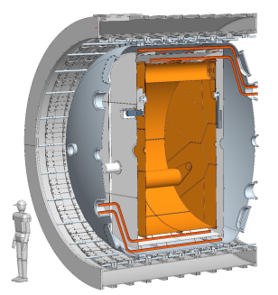
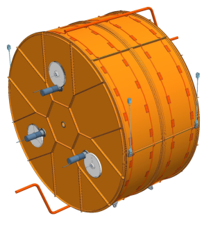
Figure 2.2: Left: Cutaway picture of the KLASH haloscope. Right: The KLASH resonant cavity.

Two different resonant cavities are foreseen to investigate the axion mass region between 0.3 and 1 $\mu$eV. They are cylindrical with length 2041 mm and radius 1,860 mm and 900 mm.

Table 2.1: The KLASH geometry

Parameter	Value
LLargeCavity [mm]	2042
RLargeCavity [mm]	1860
RLargeRod [mm]	200
LSmallCavity [mm]	2042
RSmallCavity [mm]	900
RSmallRod [mm]	100

Frequency tuning is obtained by means of three metallic rods and fins as shown in Fig. 2.3 and by replacement of the larger cavity with the a smaller one. A detailed description of the tuning procedure and of simulation results are discussed in Chap. 5.

Figure 2.3: Upper: geometry of the "rotisserie" tuning mechanism. Lower: Tuning by means of rods and fins.

Fine frequency tuning, between rod rotations, is obtained by the insertion of a dielectric rod. A similar technique will be used to avoid mode crossing. A summary of the cavity and tuning rod geometry is listed in Tab. 2.1.

Three different phases are foreseen. In the first phase, the large cavity will be tuned with three rods changing the frequency from 65 to 115 MHz. In the second phase three fins will be inserted to allow frequency tuning up to 150 MHz. Finally, the large cavity will be replaced with a smaller one to allow frequency tuning from 140 to 225 MHz. The resonant cavity must be build in oxygen-free high thermal conductivity copper (OFHC). This type of copper may show residual resistance ratios (RRR) that vary from 50 to 700. We assume RRR = 50 in the following. With this value we simulated with ANSYS-HFSS code [123] the quality factor and form factor $C_{010}$ of TM₀₁₀ mode. The results are shown in Fig. 2.4 and 2.5 as a function of the mode frequency for the three different cavity configurations. These results are used in the following section to determine the KLASH sensitivity to QCD galactic axions and Dark Photons. In Tab. 2.2 we summarize for the three different resonant cavities (Large, Large with fins, and small) the frequency range and the number of frequency steps.

Figure 2.4: Assuming copper with RRR=50

Figure 2.5: TM010 geometrical factors $C_{010}$.

Table 2.2: Summary of frequency tuning

Cavity	frequency range	number of steps
Large	65 MHz - 115 MHz	104,000
Large with fins	115 MHz - 150 MHz	44,000
Small	140 MHz - 225 MHz	85,000

As discussed in Sec. 6.1 a Microstrip SQUID Amplifier (MSA) is an optimal solution, in terms of low noise, frequency band and gain, for the first stage of signal amplification. The summary of amplification steps and equivalent temperature noise is shown in Tab. 2.3.

Table 2.3: Summary of amplification steps and equivalente noise temperature

Device	gain	Noise Temperature	operating temperature
MSA	20 dB	0.4 K	4.5 K
HFET	15 dB	5 K	4.5 K
Secondary Amplification	60 dB	150 K	300 K

2.2 The KLASH Sensitivity

The discovery potential in the coupling-mass plane is shown in Fig. 2.6. The sensitivity band reaches the band predicted for QCD axions of the KSVZ and DFSZ models.

Figure 2.6: The KLASH discovery potential (90% c.l.) compared to existing experimental limits. The red lines with yellow error-band show the theoretical predictions for the KSVZ and DFSZ axions [117, 118]. The grey area shows the prediction from other hadronic axions models [35]. The experimental limits are measured with light shining through a wall experiments [130, 131], from changes in laser polarization [132], helioscopes [133], and haloscopes [12, 13, 114, 134, 135].

We considered here an integration time of 5 minutes for a single measurement with the large Cavity and 10 minutes for measurements with large cavity with fins and small cavity. According to the estimated number of measurements in Tab. 2.2 the total integrated time will be about 3.5 years.

Table 2.4: The KLASH discovery potential for KSVZ axions. $\beta$ is chosen equal to 2 to optimize the scan rate [13].

Parameter	Value
$m_{a}$ [$\mu$eV]	0.27
$g_{a\gamma\gamma}^{KSVZ}$ [GeV-1]	$1.0\times 10^{-16}$
$P_{\mbox{sig}}$ [W]	$1.33\times 10^{-22}$
Rate [Hz]	3,050
$B_{max}$ [T]	0.6
$\beta$	2
$\tau$ [min]	5
$T_{sys}$ [K]	4.9
$g_{a\gamma\gamma}$ 90% c.l. [GeV-1]	$5.3\times 10^{-17}$

2.3 Dark Photons sensitivity

The hidden photon (HP) field $\chi_{\mu}$ describes a hidden $U(1)$ symmetry group that mixes with the photon through a Lagrange density of the form

$$\mathcal{L}_{\chi_{\gamma}}=-\frac{1}{4\mu_{0}}F_{\mu\nu}\,F^{\mu\nu}-\frac{1}{4\mu_{0}}X_{\mu\nu}\,X^{\mu\nu}+\frac{\sin\chi}{2\mu_{0}}X_{\mu\nu}\,F^{\mu\nu}+\frac{\cos^{2}\chi}{2\mu_{0}}m^{2}_{\gamma^{\,\prime}}X_{\nu}\,X^{\nu}-j_{\mathrm{em}}^{\mu}\,A_{\mu}\,,$$ (2.3)

where $X_{\mu\nu}$ is the field strength tensor, $m_{\gamma^{\,\prime}}$ the hidden photon mass, $j_{\mathrm{em}}^{\mu}$ is the electromagnetic current, $\mu_{0}$ is the permeability of the vacuum, and $\chi$ is the dimensionless mixing parameter we want to determine experimentally.

The kinetic term in Eq. (2.3) can be diagonalised by a linear transformation of the fields $X_{\mu}$ and $A_{\mu}$, and it can be chosen such that only one of the gauge fields couples to electric charges. This is an interaction eigenstate and can be then identified with the Standard Model photon. By rescaling $X_{\mu}$ and $A_{\mu}$ the kinetic terms can be put in the form with the standard normalisation, and after diagonalising the mass term, one obtains

$$\mathcal{L}_{\chi_{\gamma}}=-\frac{1}{4\mu_{0}}F_{\mu\nu}\,F^{\mu\nu}\;-\frac{1}{4\mu_{0}}X_{\mu\nu}\,X^{\mu\nu}+\frac{1}{2\mu_{0}}m^{2}_{\gamma^{\prime}}X_{\mu}\,X^{\mu}\,+j_{\mathrm{em}}^{\mu}\,(A_{\mu}+\tan\chi X_{\mu})\,,$$ (2.4)

so that the HP couples to e.m. current with strength $e\tan\chi$. Eq. (2.4) implies that for both $A_{\mu}$ and $X_{\mu}$ the Maxwell equations for the potentials are modified, and the Lorentz force becomes

$$f^{\mu}=q\,(F^{\mu\nu}+\tan\chi\,X^{\mu\nu})\,u_{\nu}.$$

This implies that an electric current also produces HP, but suppressed by a factor tan$\chi$ relative to the ordinary photon field.

The mass term can be obtained through the Stückelberg mechanism [136]. Taking $A_{\mu}$ to be real one can introduce a new real scalar field $\phi$, with the Lagrange density becoming

$$\mathcal{L}_{\chi_{\gamma}}=-\frac{1}{4\mu_{0}}F_{\mu\nu}\,F^{\mu\nu}\,+\frac{1}{2}m^{2}(A_{\mu}+\frac{1}{m}\partial_{\mu}\phi)\,(A^{\mu}+\frac{1}{m}\partial^{\mu}\phi).$$ (2.5)

This contains the term $\partial_{\mu}\phi^{\mu}/2$ which is indeed the kinetic term for a real scalar field and, furthermore, it has the mass term for a vector field.

The microwave resonant cavity experiments searching for axion can also be used to probe photon-HP mixing when operated without the magnetic field [137]. The equation of motion for the photon field $A$ then reads,

$$\partial_{\mu}\partial^{\mu}A^{\nu}=\chi\,m^{2}_{\gamma{\,\prime}}\,X^{\nu},$$ (2.6)

from which the HP field acts as a source for the ordinary photon. Expanding the e.m. field inside the cavity in terms of the cavity modes

$$\textbf{A}(x)=\sum_{i}\alpha_{i}\textbf{A}_{i}^{\mathrm{cav}}(\textbf{x}),$$

we can obtain the expression for the expansion coefficients. The asymptotic solution is found to be

$$\alpha_{i}(t)=\frac{b_{i}}{\omega_{0}^{2}-\omega^{2}-i\displaystyle{\frac{\omega\omega_{0}}{Q}}}\,\mathrm{e}^{-i\omega t}$$ (2.7)

where $b_{i}$ is the driving force and the frequency is related to the HP energy through

$$\omega=E_{\gamma{\,\prime}}\simeq m_{\gamma{\,\prime}}.$$ (2.8)

The power emission of the cavity is related to the energy stored and the quality factor of the cavity, and it is given by

$$P_{\mathrm{sig}}=\kappa\chi^{2}m_{\gamma{\,\prime}}\rho\,Q\,V\,G,$$ (2.9)

where $\kappa$ is the coupling of the cavity to the detector, $Q$ the quality factor, $V$ the volume of the cavity and the geometric factor $G$ is defined as

$$G=G_{\mathrm{axion}}\cos^{2}\theta.$$ (2.10)

Assuming the energy density of the HP to be equal to the dark matter density (0.45 GeV² cm^-3), and the same quality factor used for the axion search, and the volume of the cavity equal to 22 m³ (for the large phase of the experiment) and 5.2 m³ (for the small phase), we can use this formula to constrain the HP CDM with the KLASH microwave cavity. It is already evident that the large dimension of the cavity significantly enhance the sensitivity for HP, also thanks to the fact that no magnetic field is required for this kind of physics analysis.

Figure 2.7: Top panel - Compilation of current constraints on and sensitivities of planned experiments to photon-HP mixing in the $m\gamma^{\,\prime}-\chi$ plane. With bars in blue (red) the conservative (equally likely HP distribution) estimates for the ADMX-like haloscope search experiments [137] and the KLASH predicted sensitivity. More details are given in the text.

Typical values for the mixing parameter $\chi$ range from $\sim 10^{-2}$ down to $\sim 10^{-16}$, KLASH can further improve this value. In top panel of Fig. 2.7 is showed a compilation of current constraints on and sensitivities of planned experiments to photon-HP mixing in the $m_{\gamma^{\,\prime}}-\chi$ plane. The bottom plot of the same figure shows the predicted sensitivity of KLASH, compared to the sensitivity of an ADMX-like haloscope.

The predicted sensitivity for KLASH is computed inserting in Eq. (2.2) the $P_{\mathrm{sig}}$ obtained from Eq. (2.9). Two scenarios are possible, depending on the relative orientation of the cavity with respect to an a priori unknown direction of the HP field. This is represented by the factor $\cos^{2}\theta$ in Eq. (2.10). As a conservative estimate, assuming that all directions in space are equally likely, we can consider $\cos^{2}\theta$ such that the real value is bigger with 95% probability. In this scenario $\cos^{2}\theta=0.0025$ (showed with the histograms in blue and in the full colours in the top and in the bottom of Fig. 2.7, respectively). The other situation, considers the average over all possible directions (i.e. $\cos^{2}\theta=1/3$) and it is more optimistic. This is shown with the histogram in red and with the dashed filling in Fig. 2.7 (top and bottom).

Part II Conceptual Design

Chapter 3 Mechanical Design

3.1 Cryostat general description

A design study of the cryostat assembly has been performed by an engineering firm, under our specifications, demonstrating its technical and economic feasibility. The whole cryostat has been designed to maximize its volume with respect to the available space inside the KLOE magnet (Ø4865 x 4398 mm). The cryostat is equipped with the tools for the insertion and mounting inside the KLOE magnet.

The Cryostat includes:

• The vacuum vessel, made by a-magnetic stainless steel;

• The shield in aluminum alloy, to be cooled to 70 K by gaseous Helium;

• The resonant cavity in OFHC copper, with his tuning system, cooled to 4.6 K by saturated liquid Helium; The tuning system includes three cylindrical bars, mounted on three eccentric crank and simultaneously positioned by high precision drives with reduction gearboxes.

All the three have the two end caps flanged and are equipped with the mounting and handling tools. The shield and the cavity have a cooling circuit.

The cryostat is completed by the superinsulation layers, the cryogenic turret, all the feedthroughs for piping and cabling. Included in the design study are the main accessories for the handling. The thermal insulation of the cryostat has been analyzed, and a preliminary design of the shield, of the insulation layers and of the suspension has been done, to minimize the conduction and radiation heat exchange with the external environment. The vessel is designed to stand with the internal overpressure due to an event of helium leak.

The issues arising from the fabrication of large vessels, especially for the aluminum and copper ones, have been analyzed and their feasibility demonstrated at a reasonable cost.

3.2 Vacuum vessel

The vacuum vessel has an external diameter of 4,660 mm, maximum length of 4,480 mm and a weight of 14,000 kg (see Fig. 3.1).

Figure 3.1: The vacuum vessel.

The vessel shell (2 cm thick) is formed by four cold-rolled austenitic stainless steel plates, welded together and to the flanges. The heads (1.5 cm thick) will be realized by press-formed dishes with welded flanges; the heads are equipped by the openings for the pass-through of pipes and cables and for the mounting operation. All the welds and composed by an internal vacuum tight bead and an external structural piecewise reinforcement welding. The flanges will be milled with a precision that guarantee the vacuum tight coupling. The shell and the heads flanges are bolted together; the sealing is done by VITON O-rings.

External to the vessel will be realized the interfaces for the anchoring to the magnet, while in the internal face will be welded the supports for the suspension of the cavity and the shield.

3.3 Cryostat support

The cryostat assembly will be supported inside the KLOE magnet by means of the anchoring interfaces spaced at 15 degrees that was used for the 24 calorimeter modules, weighing 2 ton each. So, the maximum load distributed could be no more than 480 N. 24 longitudinal rails will be mounted by 9 supports each (see left panel of Fig. 3.2), using the existing screwed holes on the internal surface of the magnet, and precisely aligned by laser tracker.

Four supports will link each couple of rails to the cryostat. Each support could slide on the couple of rails by low friction sleeves (made by Frelon Gold) and will be bolted to the vessel by elastic silent-blocks (see right panel of Fig 3.2). Small alignment errors of each support could be adjusted by the eccentric pin in the middle, while the parallelism error between each couple of rails could be accommodated by the elastic blocks.

Figure 3.2: The mounting rail (left) and the support block (right).

With this arrangement, the vessel alone, without heads, could be inserted sliding along the rails in the first mounting phase.

3.4 Cavity

The cavity will be a cylinder with flat ends (Fig. 3.3), internal dimension Ø3,690 mm x 1,960 mm, external Ø3,800 mm x 2,060 mm, weight 2,600 kg.

Figure 3.3: The cavity.

The shell will be made by 12 tiles, realized by cold formed commercial plates of copper OFHC (1,000 x 2, 000 x 5 mm), joint by rivets. Circumferential ribs will enhance the rigidity of the assembly. To minimize eddy current loops, the longitudinal joint between tiles will be insulated by NEMA G10 plates and insulating sleeves. The end plates will be made by 13 tiles, cold formed and joint by rivets and screws.

The cavity will be suspended to the vessel by four stainless steel (AISI 316L) tie-rods, with a length adjustment and a heat link to the 70K shield. Some pins will keep the horizontal position of the cavity. Tie-rods and pins will be sized to minimize the heat conduction.

The cooling of the cavity will be done by a 4.6 K liquid helium circuit, made by two manifold (upper and lower) connected by Cu-DHP copper tubes in parallel. The tubes will be connected by small plates brazed to the tube and riveted to the cavity.

The cavity assembly is such to allow opening of the end plate for servicing.

3.5 Tuning system

In the cavity there three OFHC copper hollow cylinders (“tuners”, Ø400 mm for the whole length of the cavity) will be mounted on eccentric positioning devices (three motorized couples of cranks with a counterweight). The three cylinders could be positioned simultaneously at a distance from the axis of the cavity from 560 to 1,640 mm.

The electric continuity of the cavity will be assured by sliding contacts around the tuners shafts. Each tuner will be equipped by a vacuum compliant Hybrid Stepper-Motor (200 step/turn, 150 min^-1) with a three-stage epicyclical gear unit (1:200) and a gear couple (1:10). The total angular step will be $9^{-4}$ degrees. The whole turn will take around 7 min. Each motor will have a thermal probe and an angular resolver, while all the three will be driven by a control unit, external to the cryostat. The whole tuning system will weigh 1,050 kg.

Figure 3.4: Internal view of the cavity with the tuner (left); tuner assembly (right).

During the data taking, the motors will be switched off, but their position will be kept in the control memory, to avoid any further homing.

3.6 Shield

The cylindrical shield (Fig. 3.5) will be made of aluminum alloy AA 5083 H112 (Ø4,220 x 2,500 mm). It will cover the cavity without contact, while will lay on the vacuum vessel by means of sixteen adjustable pins. The shell of the shield will be made of two halves (4 mm thick) with longitudinal flanges and ribs (10 mm thick), all welded. The two flat ends end will be made by three plates bolted together. On the shield there will be bolted the covers for the tie-rods and the motors protruding from the cavity, and the shield will be thermally connected with the tie-rods. The shield will be cooled by 70 K gaseous helium circulating in a circuit similar to that described for the cavity. The total weight of the shield will be 1,000 kg.

Figure 3.5: The shield.

3.7 Mounting sequence

In the KLOE hall, a double crane with a suitable lifting capacity is available. After mounting the rails inside the magnet, the vacuum vessel shell will be inserted by a suitable mounting tool, composed by two stands and a trolley running along a rail on ball bearing mountings. The shield and the cavity shells will then be inserted by the same tool. Each shell will be aligned and put or hanged on its supports. Then the ends of the cavity will be bolted, the tuners put in position and finally the motors and the counterweights. The alignment of the components during all the mounting phases should be checked by laser tracker.

Figure 3.6: Cryostat assembly section.

After mounting all the accessories, the cryogenic feedthroughs and the insulating layers, the end caps of the shield and of the vacuum vessel will be put in position by the crane and a suitable sling.

Figure 3.7: The various phases of the insertion of the vessel: 1 (top left); 2 (top right); 3 (bottom left); 4 (bottom right).

3.8 Preliminary structural simulations

Some simulations have been performed to demonstrate the feasibility of the three main components of the cryostat. All the results are compliant with the functionality of the cryostat and the safety of the assembly, i.e. the stress values are well below the yielding, the displacement values are suitable for the functioning of the components and the assembly operations, even when the shells are lifted and mounted without the ends. A special buckling simulation has been performed to check the behavior of the vacuum vessel during vacuum leak test at the factory, i.e. without the supports inside the magnet. Finally, a check according to the ASME VIII Div. 2 (4.4.5 Cylindrical Shells) shows a permissible load of 0.53 MPa with a safety factor of about 2.

In the figures below are reported the main results of the simulations concerning displacement, stress and buckling of cavity, shield and vacuum vessel.

Figure 3.8: Top: cavity displacement (left) and stress (right) under its own weight. Bottom: cavity shell displacement under its own weight.

Figure 3.9: Top: shield displacement (left) and stress (right) under its own weight. Bottom: shield displacement (left) and stress (right) under its own weight without ends.

Figure 3.10: Vacuum vessel stress (left) and buckling (right) under vacuum.

Chapter 4 Cryogenics

4.1 The cryogenic plant

The cryogenic plant consists in LINDE TCF 50 Cold Box, a LINDE valve box and a KAESER ESD442 compressor, all connected together using a transfer line system. This plant operated at DA$\phi$NE since 1997 as a cold He supply for the KLOE and FINUDA detectors and for other four OXFORD superconducting anti-solenoids. The former KAESER compressor was replaced in 2015 with the present ESD442, which so far operated for 15000 hours.

The plant has the following nominal performance:

• Liquefaction rate = 1.14 g/s;

• Refrigeration capacity at 4.45 K/1.22 bar = 99 W;

• Shield cooling capacity below 80 K = 800 W.

The plant is able to take cold the KLOE magnet and the KLASH cryostat at the same time. The capacity request for KLOE, cold at steady state, is:

• Liquefaction rate (KLOE) = 0.3 g/s;

• Refrigeration capacity at 4.45 K/1.22 bar (KLOE) = 55 W

• Shield cooling capacity below 80 K (KLOE) = 530 W

So, the cooling capacity available for KLASH, cold at steady state, is

• Liquefaction rate (for KLASH) = 0.84 g/s;

• Refrigeration capacity at 4.45 K/1.22 bar (for KLASH) = 44 W

• Shield cooling capacity below 80 K (for KLASH) = 270 W

KLASH does not need liquefaction, so the liquefaction capacity can be roughly converted to a refrigeration value, using a conversion factor of 100 J/g [138]. In this case 84 W (0.84 g/s $\times$ 100 J/g), to be added to the real refrigeration capacity. The effective total availability become:

• Refrigeration capacity at 4.45 K/1.22 bar (for KLASH) = 128 W

• Shield cooling capacity below 80 K (for KLASH) = 270 W

If necessary, a Liquid Nitrogen line connected to the Cold Box is available to speed-up the KLOE/KLASH cool down.

A Siemens SIMATIC S7-400 PLC provide a fully automatic operation of the cooling process. A PC with a dedicated synoptic enables a complete remote view and control of the operations.

4.2 The cryogenics layout

In Fig. 4.1 a view of the proposed cryogenic layout is shown. The cryoplant Cold Box is located in the cryogenic lab. KLOE, KLASH and the Valve Box are in the KLOE hall. In red the transfer lines are depicted. The plant compressor is out of the picture. The Cold Box-Valve Box transfer line consists of 5.2 SHe/70 K GHe send/return line, all contained in a vacuum tight tube. The Valve Box-KLOE and Valve Box-KLASH lines are similar.

The Valve Box is a distribution box in which the coming 70/5.2 K He coming from the Cold Box is splitted in different lines to the users by means of cryogenic valves. At present the Valve Box is placed at the center of the DA$\phi$NE hall, so several modifications in the plant are foreseen to adapt the plant for KLASH. The Valve Box should be moved inside the KLOE hall to minimize the transfer lines path. It can be placed in the platform in place of the KLOE management gas. It must be checked if the platform can support the Valve Box and transfer lines weights

Figure 4.1: The cryogenics layout.

Following the valve box repositioning, the transfer line path on between the cold and valve boxes should be modified.

New transfer lines should be made from the Valve Box to KLOE and KLASH. Their total length is of the order of 30 meters. Their cost is estimated in 2.5 k€ per meter.

4.3 The KLASH service turret

Cold Helium from the LINDE plant flows inside the transfer lines (TL) as a supercritical gas (SHe) at 5.2-5.4 K and about 3 bars. This is preferable respect to exiting the plant directly with the liquid, because the heating generated in the TLs could produce liquid-to-gas transition that will result in larger pressure drop, worsening the heat transfer performance. To reduce the thermal noise, the cavity must be operated at the lowest possible temperature, so it will be cooled at LHe temperature (4.4 K/1.2 bar), using a service turret where the SHe will be expanded through a Joule-Thomson valve, then collected in a vessel as a liquid and distributed to the user.

The same turret will permit the gas management during the cryostat cool down and warmup, by means of mixing valves and heat exchangers.

In Fig. 4.2 the service turret scheme is depicted.

Figure 4.2: Service Turret layout.

During the first part of the cool down (from ambient temperature down to about 100 K), care must be taken to avoid excessive thermal stresses to cavity and 70 K shield. For this purpose, the cooling gas should than controlled in temperature to values no more than 50 K below the users’ average temperature. To this purpose, warm (300 K) He line is splitted in two. In the first line the gas flows unchanged while in the other it is cooled by the 70 K GHe coming from the cryoplant by means a counterflow heat exchanger. The two lines are then mixed, in order to get a temperature-controlled gas flow.

Mixed with this hydraulic scheme allows to choose the temperature of the GHe entering the cryostat at the desired value, in order to follow the cavity temperature decreasing. This shall avoid excessive thermal stresses due to temperature gradient. Due to the lack of available space inside the magnet bore and the needs to access to the valves, the service turret must be necessarily positioned outside from the KLOE iron yoke. It will be placed on the platform above the KLOE magnet. The connection pipes between the turret and the cryostat should pass through some of the through holes in the iron yoke that was formerly used for the signal cables of the KLOE detectors. The holes size (300 x 120 mm each) is such that the four He pipes (send/return of 4.5 and 70 K) cannot be hosted in a single vacuum tube. The transfer line will therefore be splitted in two smaller tubes, the first housing the 4.5/70 K send pipes end the second the 4.5/80 K return lines. In both pipes, at the warmer line will be thermally connected a radiation shield used for the colder one. In Fig. 4.3 a sketch of the transfer line section is shown.

Figure 4.3: Service Turret/cryostat He transfer line.

The turret will be supplied with Helium coming from the LINDE plant valve box, using the exit piping that was formerly used for the FINUDA magnet cooling. The turret vacuum will be in connection with the cryostat one by means of the transfer lines, so its pumping will be provided by the cryostat pumping system. A number of sensors are required to control the Helium properties. In Fig. 4.1 the position of temperature (TT), pressure (PT), liquid Helium level (LT) and flow measurement sensors (FT) are indicated. Flow sensors are positioned outside of the cryostat. Pressure sensors are placed at room temperature, connected with the vacuum tank. All the cold sensors (thermometers and level probe) shall have a spare, to allow continuous operation in case of a sensor fault.

4.4 The KLASH cryostat cryogenics

Both cavity and 70 K shield are cooled in thermal contact with lines containing the flowing Helium. The LHe and GHe send lines entering the KLASH vacuum tank go on the bottom side of the cavity and 70 K shield, respectively. The hydraulic layout is similar on both users. A collector is placed on the bottom, parallel to the user’s longitudinal axis, from which start several parallel lines going radially up to the top, where another collector takes the gas to the return lines. In Figure 4.4, a sketch of the He lines layout is shown.

Figure 4.4: Sketch of the cavity/70 K shield He lines.

4.5 The KLASH cryogenics diagnostic

All the sensors (temperature, pressure, flow, Helium level) signals are read by their respective electronics and sent to a PC running a customized Labview program. The same software controls the service turret valves, in particular the Joule-Thomson valve where the Helium liquefies. For that valve, a software proportional control manages the opening of the valve, taking the liquid level constant inside the turret vessel. A set of temperature and pressure ranges must be defined in order to create warning/alarm messages in case of anomalous values.

Chapter 5 RF

5.1 Cavity Design and Tuning

The RF design of the cavity was done using the simulation code Ansys [123] with the goal has of designing a resonant cavity working on the mode TM010 and tunable in the range $\sim$ 60-250 MHz. This wide range of tuning cannot be covered with a single cavity and we decided to implement two cavities with their own tuning systems. The first one will cover the range $\sim\leavevmode\nobreak\ 60-150$ MHz while the second one the range $\sim$ 130-250 MHz with an overlap of few tens of MHz. The two cavities have different diameter and are schematically represented in Fig. 5.1.

Figure 5.1: Sketches of the two cavities (without tuning system) proposed to cover the frequency range of resonant frequencies 60-250 MHz.

The tuning system is based on the use of metallic movable rods, as schematically represented in Fig. 5.2 where the optimized case of three rods is represented.

Figure 5.2: Sketch of the cavity with tuning system.

A similar tuning system has been already adopted in [12, 139, 140]. We have investigated different possible cases in term of number of rods, dimensions and positions and the final parameters are reported in the Table 5.1 for the two different cavities. Each rod of radius $R_{\mathrm{rod}}$ can rotate (angle $\alpha$) around the centre $C_{\mathrm{rot}}$ moving towards the center of the cavity on a circular trajectory of radius $R_{\mathrm{rot}}$. This allows tuning the mode TM010 at different frequencies with a rotation of the rods instead of a rigid translation, that is more difficult to implement in a real cavity inserted in a cryogenics system. From Table 5.1 it is also possible to note that the frequency range 116-137 MHz is not covered. We will illustrate in the following the solution proposed to cover it.

Parameter	KLASH Low Frequency	KLASH High Frequency ($S$)
$R$ cavity (mm)	1860	900
$R_{\mathrm{rod}}$ (mm)	200	100
$R_{\mathrm{rot}}$ (mm)	480	240
$C_{\mathrm{rot}}$ (mm)	1180	560
$L_{\mathrm{rod}}$ (mm)	2042	2042
n. tuning rods	3	3
Frequency range (MHz)	66 - 166	137 - 242
$Q/1000$	733 - 477	643 - 386
Form factor	0.66 - 0.76	0.65 - 0.76
BW (Hz) @ $\beta=1$	180 - 490	430 - 1250

Table 5.1: Main parameters of the two cavities with tuning system.

The contact between the rod and the parallel plates of the cavity has to be guaranteed in order to not deteriorate the quality factor. In fact, a non-perfect contact creates, in the gap, a capacitor and increases losses. Simulations have been performed and indicate that a gap of 1 mm can be tolerable and deteriorated the $Q$ factor by less than 5%. This problem has been already addressed in [139]. Different rods configurations have been explored and are schematically represented in Fig. 5.3.

Figure 5.3: Sketch of the analyzed tuning rods configurations with magnitude of the electric field.

We considered the cases of one, two and three symmetric rods exploring different radius, positions, and centres of rotation. For all configurations the frequency range, the quality factor and the form factor of the working mode have been calculated and we have finally proposed the configuration with three rods of radius $R_{\mathrm{rod}}=200$ mm, $R_{\mathrm{rot}}=480$ mm and $C_{\mathrm{rot}}=1180$ mm. This choice has been a compromise between the complexity of the system and the tunability range. Fig. 5.4 shows, as an example, the frequency of the TM₀₁₀ mode and of all other identified modes, as a function of the angle of rotation $\alpha$ for the two cases of a single rod ($R_{\mathrm{rod}}=100$ mm, $R_{\mathrm{rot}}=780$ mm and $C_{\mathrm{rot}}=980$ mm) and the final case of three rods. In the case of three rods they are moving symmetrically. The rotation angle $\alpha=0$ corresponds to the case of the rod near the cavity wall.

Figure 5.4: Frequency of the TM₀₁₀ mode and of all other identified modes, as a function of the angle of rotation $\alpha$ for the two cases of a single rod with $R_{\mathrm{rod}}=100$ mm, $R_{\mathrm{rot}}=780$ mm, and $C_{\mathrm{rot}}=980$ mm (left) and the final case of three rods with $R_{\mathrm{rod}}=200$ mm, $R_{\mathrm{rot}}=480$ mm, and $C_{\mathrm{rot}}=1180$ mm (right).

The second case is, obviously, more effective. From the plots it is quite easy to note that the proposed tuning system does not translate the frequency of all cavity modes rigidly. There are positions of the rods for which we have an overlap between different modes. We can note, as an example, the overlap between the working mode and TE modes and also with the modes due to TEM resonances of the coaxial line generated by the rod (inner conductor) and the outer wall (outer conductor) that we indicated as “TEM coaxial modes”.

The overlap between modes gives a “mode mixing” effect that could make the detection of the mode TM₀₁₀ more difficulty in the crossing region between the modes, as already pointed out in [139]. The working mode TM₀₁₀ mode will be detected through a coaxial probe inserted in one of the two end-caps of the cavity and parallel to the axis of the cavity itself, as sketched in Fig. 5.5.

Figure 5.5: Sketch of the antenna coupled to the cavity modes.

The coupling of the probe can be varied changing the penetration of the inner conductor ($L_{\mathrm{inner}}$). We verified, by simulations, that, even with a standard-SMA antenna it is possible to change the coupling $\beta$ of the antenna with the TM₀₁₀ mode, in a wide range (between 0 and 2) moving the penetration of the inner by few tens of cm. By simulations we verified that the TM₀₁₀ mode is always very well identifiable from the probes even near the crossing region between TE-TM modes. This is due to two reasons: first of all because the probe is coupled to the longitudinal electric field of the modes only (that is in principle zero for the TE and TEM modes) and, secondly, because the mode couplings between the TM₀₁₀ mode and the TE ones is very weak. This is, for instance, visible in Fig. 5.6 where the transmission coefficient between two coaxial probes coupled to the cavity is reported for different tuner positions that crosses the mode mixing region TM₀₁₀-TE₂₁₁. Also simulations in a smaller frequency range confirmed that the TM₀₁₀ is always very well detectable.

Figure 5.6: The transmission coefficient between two coaxial probes coupled to the cavity is shown for different tuner positions that cross the mode mixing region TM₀₁₀-TE₂₁₁.

Mode crossing may be resolved by proper rotation of the three tuning rods or by proper insertion of dielectric tuning rods.

The sensitivity of the resonant frequency, as a function of the rotation angle, is reported in Fig. 5.7.

Figure 5.7: Sensitivity of the resonant frequency as a function of the rotation angle is reported.

The detection of the induced signals will be done at different resonant frequencies of the cavity. The resolution in term of frequency steps that we would like to achieve is directly proportional to the bandwidth of the cavity reported in the last line of Table 5.1.

In order to achieve a resolution on the order of the mode bandwidth (or lower), as can be understood from Fig. 5.7, the required sensitivity in term of tuning angle has to be much smaller than 17.5 $\mu$rad. If we want to achieve a better sensitivity in the resonant frequency tuning, we have to add another, less sensitive, tuning system. One possibility is to insert a small cylinder of dielectric material(alumina or sapphire) as sketched in Fig. 5.8. With a cylinder of 60 mm of radius, in sapphire, we achieved, as an example, a sensitivity of 200 Hz/mm that can be further reduced decreasing the diameter of the cylinder itself.

Figure 5.8: Dielectric tuning system for fine frequency tuning.

The quality factor and of the TM₀₁₀ mode as a function of frequency and for different number of rods is given in Fig. 5.9. In the plot we supposed that the rods and the cavity

Figure 5.9: Quality factor and of the TM₀₁₀ mode as a function of frequency and for different number of rods.

are made of copper with a value of RRR equal to 20 and, as a consequence, with a conductivity at 4 K of $1.16\times 10^{9}$ S/m [141]. We also calculated the form factor [139] and the results are given in Fig. 5.10.

Figure 5.10: Form factor of TM₀₁₀ mode as a function of frequency and for different number of rods.

We also considered the case of different copper RRR (see Fig. 5.11)

Figure 5.11: Form factor of TM₀₁₀ mode as a function of frequency and for different RRR of copper.

As already pointed out, to cover the frequency range up to 250 MHz, we will substitute the cavity with another one with a smaller radius. To increase as much as possible, the frequency range to be explored we decided to choose this cavity radius in order to have a starting frequency higher than the highest frequency reachable with the cavity with larger radius. The frequency gap of about 20 MHz (see Table 5.1) between the two systems can be covered with a modification of the cavity with larger radius. As represented in Fig. 5.12,

Figure 5.12: Modification of the cavity with insertion of metallic plates to cover the range up to 150 MHz.

the cavity can be divided in three sectors through metallic plates. A similar solution was proposed in [142]. The metallic rods, also in this case, can be moved on the same circular trajectory detuning the TM₀₁₀ mode. In this condition the mode will cover a range up to 150 MHz as represented in the mode chart of Fig. 5.13.

Figure 5.13: Frequency of the TM₀₁₀ mode and of all other identified modes, as a function of the angle of rotation $\alpha$ in the case of cavity with metallic plates.

In this case, due to the presence of the metallic plates the mode ensemble is more complex but, in any case, the working mode is still very well identified. Fig. 5.14 reports the quality factor and form factor as a function of frequency for the same case.

Figure 5.14: Quality factor and form factor as a function of frequency in the case of cavity with metallic plates.

An alternative solution we explored is a cavity with the metallic plates inserted but rotated toward the outer wall of the cavity (open plates configuration) as schematically represented in Fig. 5.15.

Figure 5.15: Cavity with the metallic plates inserted but rotated toward the outer wall of the cavity (open plates configuration).

In this configuration the first frequency scan will be done covering a frequency interval close to the previous case, without plates, and the second scan will be done closing the plates (that are free to rotate) as previously illustrated. Fig. 5.16 reports the quality factor and the form factor of the modes as a function of frequency, in the case of open plates. It is worthwhile to note that these parameters are comparable, or even better, with respect the previous case without plates.

Figure 5.16: Quality factor and form factor as a function of frequency in the case of cavity with metallic plates rotated as represented in Fig. 5.15.

The last frequency range will be covered through another cavity with smaller radius and three tuning rods of radius equal to 100 mm. The cavity is schematically represented in Fig. 5.17.

Figure 5.17: Cavity with smaller radius and tuning system (left); frequency of the TM₀₁₀ mode as a function of the tuner position (right).

In the same figure we also reported the frequency of the TM₀₁₀ mode as a function of the tuner position. The complete mode mapping is given, in this case, in Fig. 5.18 with the quality and of form factors reported in Fig. 5.19.

Figure 5.18: Complete mode mapping in the case of cavity with smaller radius.

Figure 5.19: Quality (left) and form (right) factors as a function of frequency.

The sensitivity of the tuning system is finally reported in Fig. 5.20. Also for this case it is possible to add another tuning system for a more accurate frequency scan.

Figure 5.20: Sensitivity of the tuning system in the case of cavity with small radius.

Chapter 6 Signal Amplification and Acquisition

6.1 SQUID

The SQUID (Superconducting QUantum Interference Device) is the most sensitive magnetic flux detector currently available and has long been used for a wide range of low-frequency applications ([143]): from gravitational wave detection to biomagnetism, from nondestructive evaluation to magnetic resonance imaging.

More recently, SQUIDs have been used as low-noise, low-power-dissipation RF and microwave amplifiers [144]. Thanks to their low dissipation, SQUIDs and SQUID-based devices can be used down to ultracryogenic temperatures where one can take advantage of the fact that their noise scales with the temperature down to 2 - 300 mK. At lower temperatures, the coupling between the electrons in the Josephson junction shunt resistors $R_{s}$ (see Fig. 6.1) and the lattice phonons becomes very weak and the electron gas undergoes a Joule heating due to the bias current. This heating, the hot-electron effect, causes a deviation from the linear behavior of noise versus temperature and saturation of the SQUID noise [145].

Figure 6.1: Flux Locked Loop dc SQUID with input coil $L_{i}$ connected to pick-up coil $L_{p}$.

Despite this noise saturation, at frequencies below 1 GHz, the SQUID noise is more than an order of magnitude lower than that for a state-of-the-art cooled semiconductor-amplifier.

Two-stage commercial dc SQUIDs operating at 100 mK have shown in the audio frequency range an energy resolution referred to the input coil ($e=k_{\rm{B}}T_{n}/\omega_{0}$, where $\omega_{0}/2\pi$ is the operation frequency) of about 30$\hbar$ that is a factor 30 above the quantum limit.

Since dc SQUID readout electronics have been realized with open-loop bandwidth of 300 MHz and flux-locked loop bandwidth up to 130 MHz [146], the KLASH cavity readout scheme could be configured, at least for the frequency scan 65 -120 MHz, as shown in Fig. 6.1 where the $L_{p}$ coil is inserted in the cavity to pick up the magnetic field. In this case, however, the high dc magnetic field (about 0.6 T) in which the pick-up is expected to operate, would turn any micro-vibration of the apparatus into a signal out of the SQUID dynamic range. For this reason, though the operation frequency band of KLASH is considerably lower, the reference detection scheme remains that of the ADMX experiment (see Fig. 6.2).

Figure 6.2: ADMX scheme [147].

In the ADMX experiment, which has recently operated in the frequency range 645-680 MHz, a cryogenic heterojunction field-effect transistor (HFET) amplifier with a noise temperature of 2 K was initially used to amplify the signal picked up by a critically coupled antenna inserted in the cavity. Subsequently, a Microstrip SQUID Amplifier (MSA) [148] has replaced as front-end amplifier the HFET which is used as second stage amplifier (see Fig. 6.2). The MSA is an effective solution to the problem of the gain drop of the standard dc SQUID amplifier at frequencies higher than about 100 MHz. The gain drop can be explained as follows. Input coil and washer-type SQUID, separated by a thin insulating film, form a capacitor in parallel to the input coil inductance (see Fig. 6.3).

Figure 6.3: Parasitic capacitance formed by planar input coil on top of SQUID washer [149].

Because of this parasitic capacitance, the input circuit is purely inductive only at frequencies below the self-resonant frequency of the tuned circuit formed by the coil and the parasitic capacitance. At higher frequencies the signal is shorted by the parasitic capacitance. This deleterious effect can be avoided by making a virtue of the parasitic capacitance and by operating the input coil of the SQUID as a transmission line resonator (microstrip) (see Fig. 6.4).

Figure 6.4: Input coil on top of SQUID operated as a microstrip resonator by coupling input signal to one end of coil and washer, leaving the other end of the coil unconnected [149].

The signal to be amplified is applied between one end of the coil and the washer, while the other end of the coil is left open. Provided that the source impedance is greater than the characteristic impedance of the microstrip, there is a peak in the gain when the input coil accommodates approximately (but not exactly) one-half wavelength of the input signal. The frequency of operation of the amplifier is determined by the microstrip length, and thus by the number of turns of the input coil. The quality factor of the microstrip resonator, and thus the bandwidth of the amplifier, can be set by choosing an appropriate microstrip impedance. Gains over 20 dB, noise temperatures well below the bath temperature and operation frequencies from 100 MHz to 8 GHz have been achieved (see Fig. 6.5 [149]) .

Figure 6.5: Gain versus frequency for eight microstrip SQUID amplifiers. The length of the input coil (microstrip resonator) is indicated above the corresponding gain curves.

In the classical limit, the noise temperature $T_{n}$ of an MSA is expected to scale as $fT$, where $f$ is the operation frequency and $T$ the bath temperature [150] and measurements show that MSA can approach the quantum-limited performance. For example, a noise temperature $T_{n}=47$ mK has been achieved at 20 mK and 520 MHz [151] (see Fig. 6.6) where the standard quantum limit $T_{q}=hf/k_{\rm{B}}$ is about 25 mK. In the same series of measurements a $T_{n}=170$ mK has been obtained at 300 mK. By scaling with the frequency, noise temperatures of 16 mK and 82 mK are respectively expected at 50 MHz and 250 MHz, the extremes of the frequency range of interest for KLASH.

Figure 6.6: Noise temperature of input microstrip SQUID at 519 MHz vs temperature measured with a resonant source. The dashed line through the data corresponds to $T_{N}\propto T$, and the dot-dashed line indicates $T_{Q}=hf/k_{\mathrm{B}}\simeq 25$ mK. Inset is noise peak produced by LC-tuned circuit at 20 mK. The upward trend of the baseline reflects the fact that the peak in the amplifier gain is at a higher frequency. The peak at 520.4 MHz is a calibrating signal [151].

As mentioned above the bandwidth of the MSA can be set by choosing an appropriate microstrip impedance and it should be possible to cover each of the three bands planned for KLASH (65-120 MHz, 120-150 MHz, 150-250 MHz) by changing the MSA together with the cavity. In case it is not possible to cover completely a frequency band one can tune the frequency of the SMA by connecting a varactor diode between the otherwise open end of the input coil and the washer [151]. The capacitance of the diode can be varied by changing the value of the reverse bias voltage with the effect of increasing or decreasing the effective length of the microstrip and lowering or raising the peak frequency (see Fig. 6.7).

Figure 6.7: Gain vs frequency for a MSA for nine values of bias voltage applied to the varactor diode ([151])

.

For the reasons outlined, we believe that the best choice for the KLASH front-end amplification is the MSA also in view of a measurement of the thermal noise of the cavity with a non-optimized antenna. Of course, a series of preliminary tests of different SMA down to 300 mK are necessary in order to identify and characterize those that best fit the experiment requirements. ADMX used a circulator in their first experiments with the HEMT preamplifier to avoid back-action noise from the preamp entering the cavity and they kept it in the amplification chain when they switched to the MSA. Considering the lower frequencies of KLASH, the circulator should not be required [152]. Anyway, preliminary tests will be conducted with high $Q$ LC circuits that simulate the cavity load in order to evaluate the effect of the MSA back-action noise and address it with a specific circulator.

6.1.1 B Field Shielding

DC-SQUID amplifiers are very sensitive devices that must operate in a highly shielded volume. Several effects spoil the amplifier sensitivity:

• Large magnetic fields degrade device performance. The field intensity must be below the device intrinsic-noise level (1mG);

• Pick up noise from input circuit could induce variation on the induced field (0.01G) and generate spurious signals in the amplifier;

• Induced noise limits the dynamic range;

The MSA must be well thermally and mechanically anchored to provide good thermal stability and isothermality and to avoid spurious signals from antenna vibrations inside the cavity volume. Instead of the dipole antenna, a pick-up coil with wire-wound gradiometer [153] geometry could be investigated to reduce the effect of DC field variations. Finally, tight RF shielding must be ensured [154].

To shield the KLASH magnetic field, $H_{\mathrm{DC}}=0.6$ T, 6 to 7 orders of magnitude screening is needed (from 6000 Gauss to milli Gauss). Although SQUIDs can operate in larger static field (0.1 G) we show that this conservative screening can be obtained using different approaches:

• A passive scheme [153, 154];

• A quasi-active system provide by a persistent mode superconducting coil [155, 156];

• An active procedure with a negative feedback electronic circuit system [157, 158].

A. Passive Magnetic Shield

The passive magnetic-shielding approach is realized with long tubes of high-permeability or superconducting material [159]. Magnetic-field lines are diverted around a volume of interest reducing the local magnetic-field in the region within the shielded volume. The analytical expression of the magnetic-field shielded by a ‘semi-infinite’ tube, both respect to axial and transverse (radial) directions, is given in [154] for SC tubes (see Fig. 6.8)

$$H_{\mathrm{axial}}=H_{DC}\exp\left(-3.832\,\frac{z}{d}\right)\qquad\qquad H_{\mathrm{transverse}}=H_{DC}\exp\left(-1.84\,\frac{z}{d}\right),$$ (6.1)

and for $\mu$-metal tubes

$$H_{\mathrm{axial}}=H_{DC}\exp\left(-2.405\,\frac{z}{d}\right)\qquad\qquad H_{{DC}-\mathrm{transverse}}=\exp\left(-3.834,\frac{z}{d}\right).$$ (6.2)

SC and $\mu$-metal tubes are more effective in dumping axial and transverse fields, respectively.

Figure 6.8: Semi-infinite tube of radius $d$. The $z$-axis originates on the tube entrance and is oriented downward [154].

A combination of the two types of materials serves to effectively screen both transverse and axial field components [153]. In addition, an external layer of $\mu$-metal screens the inner volume from Earth magnetic-field, avoiding flux trapping in SC shields during cool down and before turning on the KLOE magnet.

We made an estimate on the magnetic shielding using the equation described above for the case of a superconducting cylinder. The MSA device is a square of size approximately $10\times 10\mbox{mm}^{2}$. We considered three cylindrical screens of diameters 18, 14, 12 mm and heights 53, 50, 48 mm with the MSA device placed at 24 mm from the top of the cylinders. The approximation of a semi-infinite tube is motivated by the small ratio between the MSA dimension and the cylinder real-length (about 5 cm) and the small demagnetization factor D = 0.079 [160]. These are reasonable dimensions and are easily integrated into the KLASH apparatus. In our analysis, the 3 concentric superconducting screens are gradually introduced and the results are shown in Fig. 6.9. In Tab. 6.1 we show the residual magnetic field $B_{MSA}$ calculated at the MSA position $z_{MSA}$ for three different shield geometries. The final result indicates that there are still 7 orders of magnitude of margin on the milligauss maximal operative limit of the MSA and well within the 10 $\mu$G limit indicated by the ADMX Collaboration, making this approach robust. We tested these conditions measuring the attenuation of the magnetic field with three Nb₃Sn cylinders as discussed later.

Figure 6.9: Attenuated magnetic field along the axis coordinate $z$ of a superconducting semi-infinite tube (see the first in Eq. (6.1)) for :1 shield (Left), 2 shields (center), and 3 shields (Right). The case of an external field $H_{DC}=0.6$ T is assumed. Geometrical setup for the three configurations are shown in Tab. 6.1.

Table 6.1: Residual magnetic field $B_{MSA}$ calculated at the MSA position $z_{MSA}$ for three different shield geometries.

	Single Shield	Two Shields	Three Shields
Cylinder diameter	18 mm	18 mm, 14 mm	12 mm, 14 mm, 18  mm
Cylinder height	53 mm	50 mm	48 mm
zMSA	24 mm	24 mm	24 mm
BMSA	0.22 G	$3\times 10^{-5}$ G	$5\times 10^{-10}$ G

As an example, the result of the measurement of the shielding factor $S$, where $S=B_{\mathrm{appl}}/B_{\mathrm{meas}}$, for a shield composed of two Nb superconductors, with critical field $H_{c}\approx 0.3$ T, covering a SQUID [153] is shown in Table 6.2. The DC field was $H_{\mathrm{DC}}=300$ G. Several orientations were considered. The setup is shown in Figure 6.10.

Table 6.2: Measured shielding-factor with magnet and input coil oriented transversally and axially [153].

Magnetic Field Orientation	Input Loop Orientation	Shielding Factor ($S$)
Axial	Transverse	$2\times 10^{11}$
Axial	Axial	$1\times 10^{12}$
Transverse	Transverse	$5\times 10^{9}$
Transverse	Axial	$2\times 10^{12}$

Figure 6.10: Main components of the SQUID holder [153].

The optimal ratio of shield length to shield radius, $L/r$, is 5.5 for a single shield [161] and 2 for three-layer screen [162]. The optimal ratio for radial-shield spacing, $\Gamma=r_{i+1}/r_{i}$, is 2. A layout of a three-layer respecting such proportions is sketched in panel (a) of Fig. 6.11.

Figure 6.11: a) View of the shield design; b) Axial shielding-factor S as a function of the radial-shield spacing ratio; c) Residual magnetic-field intensity inside along the shield axis for $\Gamma=1.1$ and $\Gamma=2$; d) Same as (c) but for different shield thickness [161].

We performed a measurement with three Nb₃Sn cylindrical tubes. Nb₃Sn has critical field $H_{c2}$ equal to 23 T suitable for screening the 0.6 T field of the KLOE magnet. Due to the low value of the lower critical field, $H_{c1}$ (Nb₃Sn) = 35 mT, the field penetrates into the superconducting Nb₃Sn bulk where a strong pinning must be present to block it. The measurement is done with a magnetic probe, a Lake Shore gaussmeter (model 425), with the Hall sensor placed into the concentric cylinder. The holder is fixed to the bottom of the insert and a Cernox thermometer is attached with varnish glue on the top-copper flange of the magnetic screens. The set-up is shown in Fig. 6.12.

Figure 6.12: a) Sketch of the Nb3Sn screens, b) photo of the gaussmeter inserted in the set of cylinders, c) bottom of the insert to be placed at the centre of the superconducting DC magnet inside the cryostat

We placed the insert in a liquid-He cryostat with flux control at the centre of a NbTi-8T DC-magnet and performed a zero-field-cooling (ZFC) procedure from 300 K to 4.2 K. After the cooling and before turning on the magnet, the value of the trapped Earth magnetic-field read by the gaussmeter was set to zero ("nulling process"). After turning on the magnet power-supply the gaussmeter was measuring a field value of 0.02 G $\pm$ 0.01 G. With temperature stable at 4.2 K we cycled the DC magnetic field from 0 T $\to$ 1 T $\to$ 0 T. The temperature was kept stable during this cycle in order to avoid lux jumps. In Fig. 6.13 we show the field measured as a function of the applied DC-field. Thanks to the strong pinning, the magnetic field is almost completely shielded for values up to 0.8 T. In the expanded view shown in panel A of Fig. 6.13 variations on the order of 0.1 G are visible. These variations are well described by the strong-pinning Bean-model [163]. When the field reaches 0.8 T there is a consistent field penetration, up to 0.5T for 1 T of applied field. This situation is still well described by Bean’s pinning model as shown in insert C of Fig.6.13.

Figure 6.13: Measured magnetic field in the internal volume of Nb₃Sn concentric-cylinders versus the applied magnetic field (insert A). Expanded view of the measured vs applied field in the 0-1 T (insert B). Trapped magnetic field profile according to the Bean model of flux-pinning [163].

In Fig. 6.14 we show the measured shielding factor $S$.

Figure 6.14: The shielding factor $S$ versus the applied magnetic field

This measure indicates that a screen of three concentric cylinders of Nb₃Sn could be used to screen efficienctly the KLOE magnetic field. The residual 10$\mu$G will be screened by the Nb case of the SQUID amplifier.

B. Quasi Active Magnetic Shield

In this configuration the experimental volume is shielded by a superconducting magnet, for example of NbTi, in a persistent condition. The system must be cooled in a zero field condition (ZFC). Multiple magnets can also be arranged. This solution was adopted by the HAYSTAC project [155, 156]. The set-up is shown in panel (a) of Fig. 6.15; in panel (b) we show the magnetic field, without any compensation, present in the region where a Josephson parametric amplifier (JPA) is placed.

Figure 6.15: Magnetic shielding of the JPA, including three persistent superconducting coils (a). $B_{0}$ vs $z$ data in HAYSTAC magnet; the axial positions of the cavity and the JPA canister are indicated in the absence of the field compensation coil [155, 156] (b).

C. Active Magnetic Shield

Active magnetic shielding is obtained by means of canceling coils, like Helmholtz coils, that reduce the external magnetic-field by generating an opposite field [157]. A magnetic sensor (see Fig. 6.16) detects the external field, the signal is digitized and a current is generated to cancel the measured field. A simple active shielding system can be done using a negative feedback circuit with a magneto-impedance effect sensor to cancel magnetic field noise from dc to higher frequency [157].

Figure 6.16: Schematic diagram of the control circuit used for the active magnetic field compensation.

6.2 Secondary Amplification

The room temperature electronics does not pose stringent requirements in term of noise due to the high power gain ($>35$ dB) (foreseen for) of the previous cryogenic stages. Commercial low noise components can therefore be used and the simplified readout scheme is shown in Fig. 6.17

Figure 6.17: Simplified diagram of readout chain at room temperature (the dashed components may not be necessary).

Three stages can be identified: a radio frequency (RF) amplifier stage, an intermediate frequency (IF) mixer stage and a near audio frequency (AF) mixer stage, the last two arranged in a double-heterodyne receiver.

The RF stage is based on low noise RF commercial amplifiers and devices with bandwidth of 500 MHz are adequate. The power gain, required to match the dynamic range of the following stages, strongly depends on the effective power of the signal and on the amplification that can be achieved by the cryogenic stages. A power gain between 30 and 60 dB may be required and two amplification stages may be needed. An equivalent noise temperature of the RF amplifier(s) up to 150 K is also acceptable. In fact with a power gain of the previous stages higher than 35 dB, the contribution of the first RF amplifier to the system noise temperature is lower than 0.05 K and, therefore, negligible. Commercial Amplifier like aptmp3-00200005-1627-D9-lN-2 by AmpliTech, Inc. or CITLF3 by Cosmic Microwave Technology, Inc. are suitable for such purpose but an R&D phase is anyhow required.

The RF amplifier is placed just outside the cryostat and the necessity to put this stage in a RF shielded cabinet to minimize external noise pick up should be carefully evaluated. The output of the RF amplifier feeds via a coaxial cable the IF stage of the double heterodyne receiver. The first component of such stage is an image rejection mixer that shift the RF signal power from the tuneable resonant frequencies of the cavity to a fixed intermediate frequency of 10.7 MHz while rejecting image noise power. The image rejection is necessary to avoid mixing off-band RF power into the IF bandwidth and the value of the intermediate frequency is chosen to be compatible with commercial devices. A mixer, like IRM10-1000 by Sirius Microwave, with an insertion loss of 7 dB and an image rejection better than 25 dB could be used for such purpose.

An IF amplifier to compensate the insertion loss of the mixer and a weakly coupled signal sampler to monitor the internal receiver power level can be introduced at the mixer output if needed.

A high selectivity crystal bandpass filter is then introduced to suppress noise power outside the final signal bandwidth. The filter is required to prevent any out-band noise components from being aliased into the signal bandwidth at the output of the following AF mixer stage and its bandwidth (probably around 30 kHz) must be chosen to be compatible with the quality factor of the resonant cavity. The global receiver transfer function is strongly dependent by such bandpass filter. The use of a thermalized enclosure box to avoid temperature fluctuation of the filter response should be evaluated. Finally, a double-balanced mixer down converts the output of the bandpass filter, eventually amplified, to near audio frequency band centred around 30 kHz.

To reach high precision in the down conversion, a frequency synthesizer with low phase noise and good frequency stability is used to generate the local frequency (LO) of the two mixers. The N5171 by Keysight, with a phase noise of -119 dBc/Hz, a frequency accuracy of $\pm\,4\times 10^{-8}$ and a long-term stability less than $\pm\,1$ ppm/year, is a good candidate. If higher frequency accuracy and stability are needed an external primary frequency standard could be used as LO reference clock.

The power spectrum of the AF mixer output is then acquired using a commercial FFT spectrum analyser. A resolution bandwidth of hundreds hertz should be reasonable to detect the excess power of the axion signal.

Chapter 7 Analysis

7.1 Introduction

In haloscopes, the axion is detected as an excess in measured power spectrum in a resonant cavity, in presence of a magnetic field. The axion mass is unknown, then the data acquisition procedure is done as a sequence of tuning of the resonant frequency in order to span a wider range of possible axion masses. The power from axion-to-photon conversion on resonance is given by Eq. (2.1), reported here for convenience:

$$P_{a}=\left(g_{\gamma}^{2}\frac{\alpha^{2}}{\pi^{2}}\frac{\hbar^{3}c^{3}\rho_{a}}{\Lambda^{4}}\right)\times\left(\frac{\beta}{1+\beta}\omega_{c}\frac{1}{\mu_{0}}B_{0}^{2}VC_{mnl}Q_{L}\right),$$

The goal of the analisys is to measure all the experimental parameters in order to define the power spectrum that best optimizes the SNR on the full frequency range.

From a different perspective, if an axion of mass $m_{a}$, corresponding to a photon frequency $\nu_{a}$, exists then it should appear as an excess on top of the noise in the final spectrum. The power produced by an axion-to-photon conversion is in any case very small: of the order of $10^{-22}$ W (in KLASH). The analysis procedure must be designed to extract the evidence of such a small signal with respect a most prominent noise due to the thermal noise and the noise introduced by the amplification chain. A big number of power spectra must be collected for each value of the resonant frequency. All these spectra are combined opportunely before the subtraction of the background contribution, obtained from the data, with the help of the modeling of the acquisition chain. Simultaneously to the power signal, other ancillary data are collected in order to study the stability of the whole system and to characterize all the components of the noise, as explained in the following. As already discussed above, KLASH is designed to cover the frequency range between 60 and 250 MHz, by using two cavities and exploiting the position of three metallic rods to modify the resonant frequency for the $TM_{010}$ mode. An additional dielectric bar is foreseen for the fine-tuning, mainly in case of mode crossing. In this chapter we will briefly describe the analysis procedure, based on the experience of [164] and [12].
Schematically, the data acquisition procedure is the following:

• The bars are moved to a new position

• The antenna critical coupling is measured and optimized

• The auxiliary parameters are measured (Q of the cavity, resonance frequency, temperatures, pressures,etc.)

• A given numbers of power spectra are acquired

Some of the auxiliary parameters are remeasured to check the stability during the data acquisition, then the procedure restart with the change to a different value of the resonance frequency. The integration time, for each value of the resonance frequency, depends on the accuracy needed to measure (or to put an upper limit on) the gamma coupling constant. Reversing the Dicke equation (see Eq. (2.2)) we have that, for a given SNR, the integration time is:

$$\tau=(SNR)^{2}\Delta\nu_{a}\,\left(\frac{k_{B}T_{sys}}{P_{a}^{2}}\right)^{2}$$

In the next sessions, we will briefly discuss how to combine the acquired power spectra in order to obtain a “global spectrum” to extract the signal. Equally important, as stated before, is the measurement of the cavity parameters. Here we will discuss briefly the procedure to measure some of them:

Q measurement: the unloaded quality factor for the TM010 mode is very important to define the power of the axions conversion signal and the relative contribution with respect to the background. The quality factor depends on the cavity geometry, so it must be measured at each step of bars tuning. In order to ensure the stability of Q, influenced by mechanical rods stability and by the electrical contact between rods and cavity walls, the measurement is performed before and after each step of the tuning. An rf sweep is generated with a VNA (Vector Network Analyser) around the resonance frequency and injected through a very weakly coupled calibration port inside the cavity volume. The Q value is obtained from the study of the transmission response. To allow this measurement the reading port (signal port) is temporarily disconnected from the acquisition chain.

Critical coupling measurement: in order to optimize the scanning rate, it is very important to have a critical coupling between the $TM_{010}$ mode and the acquisition chain. The critical coupling is achieved when the incident power in the cavity, through the reading port, is completely absorbed without reflections. An attenuated signal, through a directional coupler, is injected in the readout port and then acquired. The mechanical insertion of the dipole is adjusted in order to minimize the reflected power. Considering that the critical coupling optimization procedure is quite slow, it is reasonable to think that this operation is not done at every measurement step, but after a certain time, to be determined based on the experimental conditions and stability.

Cryogenic amplifier noise and gain measurement: the study of the noise in the cryogenic amplifier is very important because ultimately is the dominant component with respect to all the other sources of noise. The temperature noise can be measured slowly rising the physical temperature and by measuring the reflected power (in critical coupling regime) with the acquisition chain. This measurement is not compatible with the standard data acquisition and can be done only periodically. On the other hand, the stability of the noise can be checked each time the critical coupling procedure (see the previous point) is performed, looking at the stability of the minimum of the resonance curve. The gain of the amplifiers can be periodically checked injecting a small known signal in the input port of the amplification chain.

Room temperature electronics: this measurement is less critical with respect to what discussed about the cryogenic amplifier. In any case, it is important to check periodically the functioning of all the hot electronics section (amplifiers, filters, mixers) since external noise contribution could make unusable the collected data. To study the external noise one possibility is to disconnect the cryogenic amplifier from the acquisition chain and to connect the chain on an appropriate termination resistor. Excess on the acquired power spectrum is due exclusively to external perturbations. The rate at which this kind of test can be performed depends on the possibility to make noise measurement during rod movement, on the presence of external noise on the apparatus (that in any case must be reduced) and on the analysis procedure. A rescan procedure is in any case foreseen to avoid not persistent external noise.

Local oscillator stability: an essential part of the analysis procedure is the combination of power spectra eventually collected at a very different time. Both power spectra collected in subsequent bars positions and power spectra referring to the same resonance frequency but collected at a very different time must be combined in order to obtain the final global spectrum. In any case, the stability on long period of the reference clock, used in the heterodyne acquisition chain, must be guaranteed. A clock lock system GPS based must be compared periodically with independent source reference.

Other parameters: the working parameters of the apparatus must be constantly monitored. Cavity temperature, pressures, magnetic field, temperatures of the main electronics components and others are added to the power spectra acquired in order to define a set of coherent raw data.

7.2 Spectra Combination and Analysis

The main task in the analysis is to combine a big number of power spectra opportunely reweighted, in order to obtain a single spectrum sensitive to axions signal up to the desired precision level. As described in other places in this document, the acquisition is done through a double heterodyne mechanism is such a way to bring the high-frequency signal from the cavity to a much lower frequency easier to analyze with commercial electronics. For each value of the frequency, the width of the spectrum is defined by the components in the acquisition chain, in particular, the image rejection and the filters. Final width of 50 kHz in the final af (audio frequency) spectrum is reasonable to allow the use of a conventional high-speed FFT. This spectrum is subdivided in 500 bins of 100 Hz each, to build the power histogram for each acquisition. By considering that the proposed acquisition time (see Physics Reach), that is 5 minutes for the big cavity and 10 minutes for the fins mode and the small cavity, and that a typical acquisition time for a commercial FFT is in the order of 10 ms, in each step of measurement we collect order of 30000 spectra (60000 for the small cavity and the fins). These spectra must be averaged in order to obtain a single spectrum for the considered frequency (“base spectrum”). The base spectra are the raw objects considered in the following analysis. We can imagine several steps for the analysis:

• definition of bad samples and problematic bins,

• normalization of the spectra and subtraction of the baseline,

• combination of spectra centered on different frequencies,

• candidates definition and rescan,

• extraction of the confidence limit.

In the following, we will outline the general scheme of the procedure.

7.2.1 Cut on raw data and problematic bin

The specific reasons to cut some of the acquired spectra from the final data sample will be better defined during the data taking. Some of these reasons could be: too big variation of the resonance frequency before and after the spectrum measurement (Q during the acquisition cannot be considered stable), too high temperature fluctuations, not constant temperature in the hot electronics, anomalous gain in amplifiers. Most of these reasons are connected to failure in the cooling or vacuum systems. Some of them can be related to the mechanical movement of the bars. The experiment will have a slow control system to detect and fix long-stand problems, but we cannot exclude that data can be affected by transient problems. Even in good experimental conditions, some of the bins in an acquired spectrum could be affected by local and temporary problems, like electromagnetic interference. To identify problematic bins, we follow two strategies: either we compare the contains of the same frequency bin in two spectra acquired in two adjacent acquisition (for two different value of the central resonance frequency) or, if the perturbation remains also in subsequent base spectra, repeat the acquisition after a certain time. In the first case, we can identify in-time effects and exclude from the analysis the bins involved in the phenomenon. In the second case, one can imagine subdividing the integration time into different parts (for instance, in case of the big cavity, we can perform two sweeps in the full range with 2.5 minutes of integration per step, instead of 5 minutes). In such a way, the same bin will be acquired after a quite long time (order of months) and only very stable external perturbation will give a contribution to investigate further.

7.2.2 Normalization and baseline subtraction

Starting from the base spectra it is important to define the “analysis band”, in which the background baseline is calculated. Typically cuts on peripheral bins are used to exclude regions of the spectrum influenced by the sharpness of the filters used in the acquisition chain to clean-up the noise far from the central resonance value. The shape of each spectrum is influenced by the cavity noise and the cryogenic amplifier noise spectrum and the net gain of the receiver. To deduce this shape, two different procedures can be followed. In the first case, it is possible to build a model of the cavity based on lumped elements and then perform a fit to the measured spectrum. A non-perfect modelization of the device can introduce dilution of the signal, mainly in the case in which the signal of the axions spans over several bins. In the case of virialized axions, the intrinsic width of the cosmic halo signal is of about 100 Hz and then the signal should appear in 7 or 8 bins. The situation could be slightly better in case of non-thermalized axions, for which the power should be relaxed in a single bin. In any case, an alternative solution to the fit of the spectrum is the use of a digital Savitzky-Golay (SG)filter. This filter is a polynomial generalization of a moving average defined by only two parameters, W and d. The idea is that for each value, $x_{0}$, of the spectrum a least-squares d-degree polynomial fit in a W wide window is performed: the output of the filter is the value of the polynomial in $x_{0}$. Can be demonstrated [165] that this procedure is equivalent to a filter with a flat passband and a mediocre stop-band attenuation. This implies that the shape of the baseline obtained through this filter is not influenced by “fast” signals (like the excess due to axions conversions) while the structure of the noise is preserved. The optimal value for W and d must be determined from the shape of the base spectrum. Once the baseline is defined, the spectra can be normalized. The contains of each bin after normalization is obtained from a Gaussian distribution with average 1 and sigma dependent on the bin. To combine bins from different spectra appropriate weights must be assigned. The weights depend on many factors:

• instability of magnetic field, amplifiers gain, etc. in subsequent acquisitions,

• differences between the central bin (corresponding to the resonance frequency) and the bins we want to combine (this is due to the fact that, in general, the spectra are not flat),

• different thermal and electronic noise,

• different number of spectra used to define the base spectrum (in principle this number should be constant, but dead time in the acquisition chain and system failure can reduce the number of spectra stored for each frequency step).

By applying this procedure iteratively to all the spectra acquired at the various frequencies we have a single spectrum in the full range of investigation. Actually, in KLASH, we will have three of these spectra corresponding to the three different configurations of the resonant cavity.

7.2.3 Candidates and Rescan

From the global spectrum, it is possible to extract the presence of axions candidates. As already said before, the search for axions conversion can be done either in a single bin, in case of non-thermalized axions, or looking to excess in the released power in multiple bins, in case of axions with an energy spread generated by the relative motion of the earth with respect to the axion halo. In both case the search procedure is very similar:

• a threshold is defined in order to isolate candidates in the global spectrum (either in single or multiple bins),

• for all the bins passing the first threshold, a “rescan” is done to acquire more statistics for specific frequencies,

• the events surviving to the application of a new threshold after the rescan will be examined individually.

There is a small difference between the multiple bins search with respect to the single bin search. Essentially there are two effects: first the Maxwellian velocity distribution of the axions means that not all the power will be released on a pre-defined number of bins, second a simple a priori group of multiple bins in larger bins not centered on all the possible value of the frequency scanned, can have the effect of signal splitting.

In both searches, the main problem is the definition of the threshold both in the first phase and in the rescan. After the base spectra merging, for each bin the spectrum we have three relevant quantities: the power value $\delta_{i}$, the fluctuation $\sigma_{i}$ extracted from the Gaussian distribution corresponding to the bin, and the SNR $R_{i}$ . In the absence of correlations between the bins in the power distribution, the definition of the threshold depends only on these three quantities and on the desired confidence level:

$$\Theta=R_{T}-\Phi^{-1}(c_{1}),$$ (7.1)

where $R_{T}$ is the average of the SNR in the various bins while the function $\Phi$ is the cumulative distribution function of the standard normal distribution. The threshold in the rescan data depends on the new statistics acquired and, then, on the time of the rescan data acquisition. This duration depends on the level of precision needed to excluded fluctuations at a level higher with respect to the other bins. It is possible to derive a formula from the Dicke equation [164] to consider both the statistics acquired in the normal scan and in the rescan phase. From this new level of SNR obtained it is possible to define the new threshold to apply to the rescan candidates. Any survivors to the rescan phase must be examined one-by-one, checking experimental effects (for instance, by disconnecting the acquisition chain from the cavity to understand if there are effects on the hot electronics due to external noise and terminating with a resistor the two main sources of rf in the cavity, the weakly coupled port and the readout port, or by improving the electromagnetic isolation, or by checking with dedicated search the sources of electromagnetic interferences in the experimental area).

7.2.4 Limits

We have no a priori knowledge of which bin corresponds to axions mass. On the other hand, in the presence of noise, the only difference between the true signal and a power fluctuation is that the axions signal is persistent across different spectra and scans at the same frequency. The only things we can do it to evaluate the ratio between the expected signal and noise level and the sigma of the Gaussian distribution in each bin and to require to be below a given threshold: the probability to have a signal above this value can be considered as the confidence level of the measurement. Since in the analysis procedure for each bin different values of $\sigma_{i}$ are obtained, due to experimental effects and different statistics collected (for instance due to the rescan procedure) the exclusion limit will depend on the position of the bin considered.

7.3 Computing

Although the information collected in every single acquisition is relatively small and simple, the huge quantity of spectra needed to search for a fluctuation greater than the spectral baseline at the desired confidence level requires the definition of a strategy for the storage and data processing. In Tab. 2.2 in Sec. 2.1, the total number of steps needed to complete the scan in the range accessible by KLASH is presented. The total of the steps is around 230000. Each base spectrum is obtained from the average of 30000 or 60000 spectra, for a total of the order of $10^{10}$ single spectra produced. In addition, ancillary information must be stored in the raw data needed by the analysis. It is difficult to establish a priori the correct number of this information (temperatures, pressures, resonance frequency, amplifiers gain, etc.) but it is something in the order of 10 words of 32 bits that means the order of 1 Gb of storage. The dimension of the single spectrum depends on the digitizer. If we want to have a spectrum 50 kHz wide with 100 Hz wide signal, a factor of 10 in the digitization in order to avoid structures due to axions conversion is probably needed. By assuming 1 kHz and an ADC of 16 bits, we have that a single spectrum is 80 kb. This means that the total space needed for the storage is 1100 TB, a quantity not easy to be managed. Moreover, we are assuming a commercial FFT, while other solution can be adopted. One possibility is to use a dedicated fast digitizer with the possibility to have more information on the spectrum and apply FFT and filters in software. Obviously, this solution while increasing further the quantity of data to be acquired. A solution to this problem is to design a system to have an online pre-processing during data acquisition, exploiting the RAM of the PC as a temporary buffer. The easier things to do in this pre-processing is to perform the average of the single spectra to obtain the base spectrum, but, eventually, also other steps of the proposed analysis can be moved in the online part (for instance the algorithm for the identification of the problematic bins). Probably the time needed to move the bars between two steps in the procedure is enough to accommodate the online processing. If this time is not sufficient we can think to parallelize the processing of the step N-1 while we start to acquire the data for the step N. Additional more complex processing (as for instance the FFT in software) would benefit on the graphics processing units (GPU) processing in order to allow a fast processing in real-time without back pressure on the digitizer.

Part III Bibliography

References

- [1] R.D. Peccei and H.R. Quinn, Phys. Rev. Lett. 38 (1977) 1440.
- [2] R.D. Peccei and H.R. Quinn, Phys. Rev. D 16 (1977) 1791.
- [3] S. Weinberg, Phys. Rev. Lett. 40 (1978) 223.
- [4] F. Wilczek, Phys. Rev. Lett. 40 (1978) 279.
- [5] A. Ringwald, L. J. Rosenberg, and G. Rybka, in Particle Data Group, Phys. Rev. D 98, 030001 (2018).
- [6] I. G. Irastorza and J. Redondo, Prog. Part. Nucl. Phys. 102 (2018) 89 [1801.08127].
- [7] A. Aloisio et al. (KLOE Collab.) LNF-92/019(IR) (1992) (freely avalaible at http://www.lnf.infn.it/sis/preprint) .
- [8] M. Agnello et al (FINUDA Collaboration) LNF-95/024 (IR) (1995) (freely avalaible at http://www.lnf.infn.it/sis/preprint).
- [9] P. Sikivie, Phys. Rev. Lett. 51, 1415 (1983); Phys. Rev. D 32, 2988 (1985).
- [10] D. Alesini et al [1707.06010].
- [11] Report Fantini-Sud (private report).
- [12] S. Asztalos et al., Phys. Rev. D 64 (2001) 092003; S.J. Asztalos et al., Phys. Rev. Lett. 104 (2010) 041301.
- [13] S. Al Kenany et al., Nucl. Instrum. Methods A 854 (2017) 11; B. M. Brubaker et al., Phys. Rev. Lett. 118 (2017) 061302.
- [14] R. Barbieri et al., Phys. Dark Univ. 15, 135 (2017); N. Crescini et al., Eur. Phys. J. C (2018) 78:703; D. Alesini et al., Phys. Rev. D 99, 101101(R) (2019).
- [15] S. Chaudhuri, K. D. Irwin, P. W. Graham, and J. Mardon, [1904.05806].
- [16] M. Silva-Feaver, S. Cahuduri, H.-M. Cho, C. Dawson, P. Graham et al, [1610.09344].
- [17] L. F. Abbott and P. Sikivie, Phys. Lett. B 120 (1983) 133.
- [18] M. Dine and W. Fischler, Phys. Lett. B 120 (1983) 137.
- [19] J. Preskill, M. B. Wise, and F. Wilczek, Phys. Lett. B 120 (1983) 127.
- [20] V. B. Klaer and G. D. Moore, JCAP 1710 (2017) 043 [1707.05566].
- [21] V. B. Klaer and G. D. Moore, JCAP 1711 (2017) 049 [1708.07521].
- [22] M. Gorghetto, E. Hardy, and G. Villadoro, JHEP 07 (2018) 151 [1806.04677]
- [23] A. Vaquero, J. Redondo, and J. Stadler, JCAP 1904 (2019) 012 [1809.09241].
- [24] P. Svrcek, [hep-th/0607086].
- [25] P. Svrcek and E. Witten, JHEP 06 (2006) 051 [hep-th/0605206].
- [26] A. Arvanitaki, N. Craig, S. Dimopoulos, S. Dubovsky, and J. March-Russell, Phys. Rev. D 81 (2010) 075018 [0909.5440].
- [27] A. Arvanitaki, S. Dimopoulos, S. Dubovsky, N. Kaloper and J. March-Russell, Phys. Rev. D 81 (2010) 123530 [0905.4720].
- [28] T. Higaki and F. Takahashi, JHEP 11 (2012) 125 [1208.3563].
- [29] M. Cicoli, J. Conlon, and F. Quevedo, Phys. Rev. D 87 (2013) 043520 [1208.3562].
- [30] M. Cicoli, M. Goodsell, and A. Ringwald, JHEP 10 (2012) 146 [1206.0819].
- [31] T. Higaki, K. Nakayama, and F. Takahashi, JHEP 07 (2013) 005 [1304.7987].
- [32] M. J. Stott, D. J. E. Marsh, C. Pongkitivanichkul, L C. and Price, B. S. Acharya, Phys. Rev. D 96 (2017) 083510 [1706.03236].
- [33] L. Visinelli and S. Vagnozzi, Phys. Rev. D 99 (2019) 063517 [1809.06382].
- [34] W. H. Kinney, S. Vagnozzi, and L. Visinelli, Class. Quant. Grav. 36 (2019) 117001 [1808.06424].
- [35] L. Di Luzio, F. Mescia, and E. Nardi, Phys. Rev. Lett. 118 (2017) 031801 [1610.07593].
- [36] L. Di Luzio, F. Mescia, and E. Nardi, Phys. Rev. D 96 (2017) 031801 [1610.07593].
- [37] L. Di Luzio, F. Mescia, and E. Nardi, Phys. Rev. Lett. 120 (2018) 261803 [1712.04940.
-
[38]
G. G. Raffelt, [hep-ph/9502358].
https://inspirehep.net/record/392944/files/Pages_from_C95-01-22–1_159.pdf - [39] G. G. Raffelt, J. Phys. A 40 (2007) 6607 [hep-ph/0611118].
- [40] P. Sikivie, Lect. Notes Phys. 741 (2008) 19 [astro-ph/0610440].
- [41] J. E. Kim and G. Carosi, Rev. Mod. Phys. 82 (2010) 557 [0807.3125].
- [42] O. Wantz and E. P. S. Shellard, Phys. Rev. D 82 (2010) 123508 [0910.1066].
- [43] M. Kawasaki and K. Nakayama, Ann. Rev. Nucl. Part. Sci. 63 (2013) 69 [1301.1123].
- [44] D. J. E. Marsh, Phys. Rept. 643 (2016) 1 [1510.07633].
- [45] J. E. Kim, [1703.03114].
- [46] C. Bonati, M. D’Elia, M. Mariti, G. Martinelli, M. Mesiti, F. Negro et al., JHEP 03 (2016) 155 [1512.06746].
- [47] S. Borsanyi, M. Dierigl, Z. Fodor, S. D. Katz, S. W. Mages, D. Nogradi et al., Phys. Lett. B 752 (2016) 175 [1508.06917].
- [48] S. Borsanyi et al., Nature 539 (2016) 69 [1606.07494].
- [49] P. Petreczky, H.-P. Schadler, and S. Sharma, Phys. Lett. B 762 (2016) 498 [1606.03145.
- [50] D. J. Gross, R. D. Pisarski, and L. G. Yaffe, Rev. Mod. Phys. 53 (1981) 43.
- [51] P. Fox, A. Pierce, and S. D. Thomas, [hep-th/0409059].
- [52] M. J. Turner, Phys. Rev. D 33 (1986) 889.
- [53] K. J. Bae, J.-H. Huh, and J.E. Kim, JCAP 0809 (2008) 005 [0806.0497].
- [54] O. Wantz E. P. S. and Shellard, Nucl. Phys. B 829 (2010) 110 [0908.0324].
- [55] P. Di Vecchia and G. Veneziano, Nucl. Phys. B 171 (1980) 253.
- [56] G. Grilli di Cortona, E. Hardy, J. Pardo Vega, and G. Villadoro, JHEP 01 (2016) 034 [1511.02867].
- [57] E. W. Kolb, Edward and M. S. Turner, Front. Phys. 69 (1990) 1.
- [58] A. Vilenkin and A. E. Everett, Phys. Rev. Lett. 48 (1982)1867.
- [59] D. Harari and P. Sikivie, Phys. Lett. B 195 (1987) 361.
- [60] A. Vilenkin and E. P. S. Shellard, Cosmic Strings and Other Topological Defects. Cambridge University Press, 2000.
- [61] R. A. Battye and E. P. S. Shellard, Nucl. Phys. B 423 (1994) 260 [astro-ph/9311017].
- [62] R. A. Battye and E. P. S. Shellard, Phys. Rev. Lett. 73 (1994) 2954 [astro-ph/9403018].
- [63] M. Yamaguchi, M. Kawasaki, and J. Yokoyama, Phys. Rev. Lett. 82 (1999) 4578 [hep-ph/9811311].
- [64] M. Yamaguchi, J. Yokoyama, and M. Kawasaki, Phys. Rev. D 61 (2000) 061301 [hep-ph/9910352].
- [65] T. Hiramatsu, M. Kawasaki, and K. Saikawa, JCAP 1108 (2011) 030 [1012.4558].
- [66] T. Hiramatsu, M. Kawasaki, K. Saikawa, and T. Sekiguchi, JCAP 1301 (2013) 001 [1207.3166].
- [67] T. Hiramatsu, M. Kawasaki, K. Saikawa, Sekiguchi, Phys. Rev. D 85 (2012) 105020 [1202.5851].
- [68] G. F. Giudice, E. W. Kolb, and A. Riotto, Phys. Rev. D 64 (2001) 023508 [hep-ph/0005123].
- [69] P. W. Graham and A. Scherlis, Phys. Rev. D 98 (2018) 035017 [1805.07362].
- [70] F. Takahashi, W. Yin, and A. H. Guth, Phys. Rev. D 98 (2018) 015042 1805.08763.
- [71] T. Tenkanen and L. Visinelli, JCAP 1908 (2019) 033 [1906.11837].
- [72] S. Hoof, F. Kahlhoefer, P. Scott, C. Weniger, and M. White, JHEP 03 (2019) 191 [1810.07192].
- [73] GAMBIT collaboration (P Athron et al.), Eur. Phys. J. C 77 (2017) 784 [1705.07908].
- [74] The GAMBIT Dark Matter Workgroup collaboration (T. Bringmann et al.), Eur. Phys. J. C 77 (2017) 831 [1705.07920].
- [75] P. J. Steinhardt and M. S. Turner, Phys. Lett. B 129 (1983) 51.
- [76] G. Lazarides, C. Panagiotakopoulos, and Q. Shafi, Phys. Lett. B 192 (1987) 323.
- [77] G. Lazarides, R. K. Schaefer, D. Seckel, and Q. Shafi, Nucl. Phys. B 346 (1990) 193.
- [78] M. Kawasaki, T. Moroi, and T. Yanagida, Phys. Lett. B 383 (1996) 313 [hep-ph/9510461].
- [79] L. Visinelli and P. Gondolo, Phys. Rev. D 80 (2009) 035024 [0903.4377].
- [80] L. Visinelli and P. Gondolo, Phys. Rev. D 81 (2010) 063508 [0912.0015].
- [81] L. Visinelli, Phys. Rev. D 96 (2017) 023013 [1703.08798].
- [82] L. Visinelli and J. Redondo, [1808.01879].
- [83] P. Draper, J. Kozaczuk, and J.-H. Yu, Phys. Rev. D 98 (2018) 015028 [1803.00015].
- [84] A. E. Nelson and H. Xiao, Phys. Rev. D 98 (2018) 063516 [1807.07176].
- [85] N. Ramberg and L. Visinelli, [1904.05707].
- [86] N. Blinov, M. J. Dolan, P. I. Draper, and J. Kozaczuk, [1905.06952].
- [87] P. Jordan, Schwerkraft und Weltall: Grundlagen der theoretische Kosmologie, vol. 107. Vieweg. (Braunschweig: und Sohns), 1955.
- [88] M. Fierz, Helv. Phys. Acta 29 (1956) 128.
- [89] C. Brans and R. H. Dicke, Phys. Rev. 124 (1961) 925.
- [90] R. Catena, N. Fornengo, A. Masiero, M. Pietroni, and F. Rosati, Phys. Rev. D 70 (2004) 063519 [astro-ph/0403614].
- [91] R. Catena, N. Fornengo, M. pato, L. Pieri, and A. Masiero, Phys. Rev. D 81 (2010) 123522 [0912.4421].
- [92] M. T. Meehan and I. B. Whittingham, JCAP 1512 (2015) 011 [1508.05174].
- [93] L. Visinelli and P. Gondolo, Phys. Rev. D 91 (2015) 083526 [[1501.02233].
- [94] B. Dutta, E. Jimenez, and I. Zavala, JCAP 1706 (2017) 032 [1612.05553].
- [95] B. Dutta, E. Jimenez, and I. Zavala, [1708.07153].
- [96] L. Visinelli, Symmetry 10 (2018) 546 1710.11006.
- [97] B. Dutta, C. S. Fong, E. Jimenez, and E. Nardi, JCAP 1810 (2018) 025 [1804.07676].
- [98] G. C. Raffelt, Phys. Lett. B 166 (1986) 402.
- [99] G. C. Raffelt, in Axions: Theory, Cosmology, and Experimental Searches, pp. 51-71, Springer Berlin Heidelberg, Berlin, Heidelberg, 2008.
- [100] N. Viaux, M. Catelan, P. B. Stetson, G. Raffelt, J. Redondo, A. A. R. Valcarce et al., Phys. Rev. Lett. 111 (2013) 231301 [1311.1669].
- [101] M. Giannotti, I. G. Irastorza, J. Redondo, A. Ringwald, and K. Saikawa, JCAP 1710 (2017) 010 [1708.02111].
- [102] Z. Berezhiani, D. Comelli, and F. L. Villante, Phys. Lett. B 503 (2001) 362 [hep-ph/0009290].
- [103] M. Giannotti, Int. J. Mod. phys. A 20 (2005) 2454 [astro-ph/0504636].
- [104] T. D. Lee and C.-N. Yang, Phys. Rev. 104 (1956) 254.
- [105] B. Holdom, Phys. Lett. 166B (1986) 196.
- [106] S. L. Glashow, Phys. Lett. 167B (1986) 35.
- [107] M. Yu. Khlopov, G. M. Beskin, N. E. Bochkarev, L. A. Pustylnik, and S. A. Pustylnik, Sov. Astron. 35 (1991) 21.
- [108] PLANCK collaboration (N. Aghanim et al.) [1807.06209].
- [109] S. Dodelson and M. S. Turner, Phys. Rev. D 46 (1992) 3372.
- [110] V. A. Rubakov, JETP Lett. 65 (1997) 621 [hep-ph/9703409].
- [111] Z. Berezhiani, L. Gianfagna, and M. Giannotti, Phys. Lett. B 500 (2001) 286 [hep-ph/0009290].
- [112] L. Gianfagna, M. Giannotti, and F. Nesti, JHEP 10 (2004) 044 [hep-ph/0409185].
- [113] A. Hook, Phys. Rev. Lett. 120 (2018) 261802 [1802.10093].
- [114] B. T. McAllister et al., Phys. Dark Univ. 18 (2017) 67.
- [115] W. Chung, PoS CORFU 2015, 047 (2016).
- [116] S. Arguedas Cuendis et al., [1903.04323].
- [117] J. Kim, Phys. Rev. Lett. 43, 103 (1979); M. A. Shifman, A. I. Vainshtein, and V. I. Zakharov, Nucl. Phys. B 166, 493 (1980).
- [118] M. Dine, W. Fischler, and M. Srednicki, Phys. Lett. B 104, 199 (1981); A. P. Zhitnitskii, Sov. J. Nucl. Phys. 31, 260 (1980).
- [119] R. H. Dicke, Rev. Sci. Instrum. 17 (7), 268 (1946).
- [120] P. Franzini and M. Moulson, Annu. Rev. Nucl. Part. S. 56,207-251 (2006).
- [121] J. S. H. Ross et al., “Progress in the design, manufacturing and testing of the KLOE solenoid for the DANE ring at Frascati”. 1997 Particle Accelerator Conference, Vancouver (Canada) 12-16 May 1997.
- [122] M. Modena, “The DaNE Cryogenic System”, LNF-97/046(IR) (1997).
- [123] https://www.ansys.com/
- [124] J. C. Bardin et al., “Silicon Germanium Cryogenic Low Noise Amplifiers”, IOP Conf. Series: Journal of Physics: Conf. Series 834, 012007 (2017) .
- [125] B. Ivanov et al., Rev. Sci. Instrum. 82(10), 104705 (2011).
- [126] M.W. Pospieszalski, IEEE Microwave Magazine 6, n. 3, 62 (2005).
- [127] R. Jaklevic et al., Phys. Rev. Lett. 12, 159 (1964).
- [128] ADMX collaboration (S. J. Asztalos et al.), Nucl. Instrum. Methods A 656, 39 (2011) [arXiv:1105.4203]
- [129] C. Hilbert and J. Clarke, J. Low Temp. Phys. 61, 263 (1985).
- [130] K. Ehret et al. (ALPS Collab.), Phys. Lett. B 689, 149 (2010).
- [131] R. Ballou, G. Deferne, M. Finger, M. Finger, L. Flekova, J. Hosek, S. Kunc, K. Macuchova, K. A. Meissner et al. (OSQAR Collab.), Phys. Rev. D92, 092002 (2015).
- [132] F. Della Valle et al. (PVLAS Collab.), Eur. Phys. J. C76, 24 (2016).
- [133] M. Arik et al. (CAST Collab.), Phys. Rev. D 92 (2015) 021101 ; V. Anastassopoulos et al. (CAST Collab.), Nature Physics 13 (2017) 584.
- [134] S. DePanfilis et al., Phys. Rev. Lett. 59 (1987) 839; W. Wuensch et al., Phys. Rev. D40 (1989) 3153.
- [135] C. Hagmann, P. Sikivie, N. S. Sullivan, and D. B. Tanner, Phys. Rev. D42 (1990) 1297.
- [136] E. Stückelberg, Helv. Phys. Acta 11 (1938) 211; Helv. Phys. Acta 11 (1938) 299.
- [137] P. Arias, D. Cadamuro, M. Goodsell, J. Jaeckel, J. Redondo, and A. Ringwald, JCAP 1206 (2012) 013 [1201.5902].
- [138] M.A. Green, “The Cost of Helium Refrigerators and Coolers for Superconducting Devices as a Function of Cooling at 4 K”, LBNL Publications.
- [139] D. Lee, W. Chung, and Y. K. Semertzidis, in Proc. of 11th Patras Workshop on Axions, WIMPs and WISPs, Axion-WIMP 2015, Zaragoza, Spain, June 22-26, 2015.
- [140] I. Stern et al, Rev. Sci. Instr. 86 (2015)123305.
- [141] G. E. H. Reuter and E. H. Sondheimer, Proc. R. Soc. Lond. A 195 (1948) 336.
- [142] J. Jeong et. al, Phys. Lett. B777 (2018) 412.
- [143] J. Clarke and A. I. Braginski, The SQUID Handbook: Fundamentals and Technology of SQUIDs and SQUID Systems, vol I, Wiley-VCH, (2004)
- [144] M. Mück, M. O. Andre, J. Clarke, J. Gail, and C. Heiden, Appl. Phys. Lett., 72 (1998) 2885.
- [145] A. Vinante, P. Falferi, R. Mezzena, and M. Mück, Phys. Rev. B75 (2007) 104303.
- [146] D. Drung, C. Assmann, J. Beyer, M. Peters, F. Ruede, and Th. Schurig, IEEE Trans Appl. Supercond. 15 (2) (2005) 777.
- [147] N. Du, N. Force, R. Khatiwada, E. Lentz, R. Ottens et al., Phys. Rev. lett. 123 (2018) 151301.
- [148] M. Mück and R. McDemott, Supercond. Sci. Technol. 23 (2010) 093001.
- [149] M. Mück, J. Clarke, and C. Welzel, Appl. Phys. Lett. 82 (2003) 3266.
- [150] M. Mück, J. B. Kycia, and J. Clarke, Appl. Phys. Lett. 78 (2001) 967.
- [151] M. Mück, M. O. André, J. Clarke, J. Gail, and C. Heiden, Appl. Phys. Lett. 75 (1999) 3545.
- [152] F. J. Schupp, N. Ares, A. Mavalankar, J.Griffiths, G. A. C. Jones et al., [1810.05767].
- [153] K. W. Rigby, D. Marek, and T. C. P. Chui, Rev. Sci. Instr. 61 (1990) 834.
- [154] J. R. Claycomb and J. H. Miller, Rev. Sci. Instr. 70 (1999) 4562.
- [155] B. M. Brubaker, PhD Thesis, Yale University [1801.00835].
- [156] S. Al Kenany, M. A. Anil, K. M. Backes, B. M. Brubaker, S. B. Cahn, G. Carosi et al., Nucl. Instr. Meth. A 854 (2017) 11 [1611.07123].
- [157] Y. Okazaki, S. Yanase, and N. Sugimoto, Int. J. Appl. Elect. Mech. 13 (2002) 437.
- [158] B. Hilgenfeld, E. Strahmel, H. Nowak, and J. Haueisen, Physiol. Meas. 24 (2003) 661.
- [159] B.-X Xu and W. O. Hamilton, Rev. Sci. Instr. 58 (1987) 311.
- [160] R. B. Goldfarb and J. V. Minervini, Rev. Sci. Instrum. 55 (1984) 761.
- [161] T. J. Sumner, J. M. Pendleton, and K. F. Smith, J. Phys. D 20 (1987) 1095.
- [162] E. A. Burt and C. R. Ekstrom, Rev. Sci. Instr. 73 (2002) 2699.
- [163] C. P. Bean, Rev. Mod. Phys. 36 (1964) 31.
- [164] B. M. Brubaker, L. Zhong, S. K. Lamoreaux, K. W. Lehnert, and K. A. van Bibber, Phys. Rev. D 96 (2017), 123008 [1706.08388].
- [165] A. Savitzky and M. J. E. Golay, Anal. Chem. D 36 (1964) 1627.