Balance functions of charged hadron pairs $(\pi,K,p)\otimes(\pi,K,p)$ in Pb–Pb collisions at $\sqrt{s_{{}_{\rm NN}}}=$2.76 TeV

by

Jinjin Pan
DISSERTATION

Submitted to the Graduate School

of Wayne State University,

Detroit, Michigan

in partial fulfillment of the requirements

for the degree of

DOCTOR OF PHILOSOPHY

2019

MAJOR: Physics Approved By:

$\overline{\mathrm{Advisor^{\vphantom{\frac{I}{I}}}}\qquad\qquad\qquad\qquad\qquad\mathrm{Date}\hskip 39.12253pt}$

$\overline{\hskip 221.93158pt}$

$\overline{\hskip 221.93158pt}$

$\overline{\hskip 221.93158pt}$

DEDICATION

I dedicate this dissertation to my parents, my grandparents and my wife, for giving me courage to conquer all the difficulties, for giving me strength to embrace changes in my life, and for giving me hope to chase a brighter future.

ACKNOWLEDGMENTS

I owe a great deal of gratitude to my PhD advisor Dr. Claude Pruneau for his guidance, mentorship and patience throughout the whole process of my PhD program.

I would also like to thank the members of my PhD Committee, Dr. Sergei Voloshin, Dr. Chun Shen, Dr. Scott Pratt for their support and valuable suggestions.

And I am extremely grateful for the invaluable help from Dr. Takafumi Niida, Dr. Ron Belmont, Dr. Sumit Basu, and Victor Gonzalez, who often sit with me for hours digging the code or solving my analysis problems.

I wish to express my warm and sincere thanks to Dr. Kolja Kauder, Dr. Joern Putschke, Dr. Rosi Reed, Dr. W.J. Llope, Dr. Raghav Elayavalli, Dr. Maxim Konyushikhin, Dr. Shanshan Cao for all their help and suggestions.

I thank my fellow grad students Dr. Mohammad Saleh, Dr. Chris Zin, Nick Elsey, Isaac Mooney, Amit Kumar for fruitful discussions and fun time together.

Many thanks to the ALICE Collaboration for all the support and help.

This work has been supported in part by the Office of Nuclear Physics at the United States Department of Energy (DOE NP) under Grant No. DE-FOA-0001664.

Jinjin Pan             

CHAPTER 1   Introduction

1.1   Understanding Hadron Productions in Relativistic Heavy Ion Collisions

The two-wave quark production scenario [1] proposes that there are two waves of light quark production in relativistic heavy ion collisions. The first wave takes place within $\approx$1 fm/$c$ immediately after the beginning of a collision when gluons of the system thermalize and form a Quark Gluon Plasma (QGP). This first wave is then followed by a period of (nearly) isentropic expansion that lasts for 5-10 fm/$c$. During this period, the newly formed QGP expands longitudinally, to a lesser extent transversely, and cools down. Little charge production occurs during this stage but, eventually, as the QGP temperature drops to approximately 160 MeV, gluon collisions quickly yield a large burst of quark production. These quarks then rapidly combine to yield hadrons as the QGP transitions into a short lived hadron phase which expands further but quickly ends up streaming into free hadrons. Pratt and collaborators argued that the vast majority of charge production, based on light $u$ and $d$ quarks and yielding mostly pions, takes place during the second wave. They additionally argued that the production of strange and heavier quarks should predominantly occur during the first stage. Pratt et al. further articulated that the two waves of charge creation can be studied with general charge balance functions of identified particle pairs such as pion pairs, kaon pairs, proton antiproton pairs, proton/$K^{-}$ pairs, etc. As such, they argued, measurements of general charge balance functions (BF) shall provide quantitative insight into the time of formation of quarks, the longitudinal and transverse expansion dynamics of the QGP, as well as its quark/hadron chemistry.

In this work, we present extensive measurements of BFs of charged hadron pairs $(\pi,K,p)\otimes(\pi,K,p)$ in Pb–Pb collisions at $\sqrt{s_{{}_{\rm NN}}}=$2.76 TeV. These BF results provide new and challenging constraints for theoretical models of the production and evolution of the quark gluon plasma, as well as hadron production and transport in relativistic heavy-ion collisions.

1.2   Summary of the Objectives Of This Work

The scientific objectives of this work are established based on the state of knowledge of collision dynamics and, in particular, general balance functions described in Sec. 2.2.1, 2.2.2, 2.2.3. They can be summarized as follows: Measure and use general balance functions to …

• test the two-wave quark production scenario in relativistic heavy ion collisions,

• study the collision dynamics of large relativistic collisional systems and better constrain models of these systems,

• study the evolution of the hadron pairing probability vs. collision centrality in relativistic heavy ion collisions.

These generic goals are pursued with the following specific objectives and measurements

• establish sound procedures to measure BFs as functions of $\Delta y$ and $\Delta\varphi$,

• measure balance functions $B(\Delta y,\Delta\varphi)$ of charged hadron pairs $(\pi,K,p)\otimes(\pi,K,p)$ in Pb–Pb collisions for specific transverse momentum ranges of these hadrons,

• measure the collision centrality evolution of these BFs in Pb–Pb collisions,

• study the evolution of the longitudinal and azimuth widths of these BFs vs. collision centrality in Pb–Pb collisions,

• study the evolution of the integral of these BFs vs. collision centrality in Pb–Pb collisions.

1.3   Organization and Structure of This Dissertation

Chapter 2 introduces the notion of correlation functions and balance functions and presents a brief literature survey of recent theoretical and experimental works on balance functions. The details of the analysis method, the datasets, the optimization techniques used, and the various checks performed are described in Chapter 4, while Chapter 5 presents a detailed discussion of systematic uncertainties. The results are presented and discussed in Chapter 6. The conclusions of this work are summarized in Chapter 7.

CHAPTER 2   Balance Functions

Section 2.1 introduces the notations and observable definitions used throughout this work. In particular, it introduces the definition of the $R_{2}^{\alpha\beta}$ correlator, linear combinations of unlike- and like-sign charge combinations of this correlator, as well as the charge dependent correlator, $R_{2}^{\alpha\beta,CD}$, used in this work to determine general balance functions $B^{\alpha\beta}$.

Sections 2.2.1 – 2.2.3 present a brief literature survey of theoretical and prior experimental works on BFs. They define the historical and practical context of this study and establish the formal scientific goals of the work.

2.1   Definitions and Notations

2.1.1   Particle Number Densities

The momentum $\vec{p}$ of particles is decomposed into transverse momentum $p_{\rm T}$, rapidity $y$, and azimuthal angle $\varphi$ components:

$$p_{\rm T}=\sqrt{p_{x}^{2}+p_{y}^{2}},$$ (2.1)

$$y=\frac{1}{2}\ln\left(\frac{E+p_{z}c}{E-p_{z}c}\right),$$ (2.2)

$$\varphi=\tan^{-1}\left(\frac{p_{y}}{p_{x}}\right).$$ (2.3)

Whenever the identity of particle species is unknown, the pseudorapidity, $\eta$, is used as proxy to their rapidity $y$.

$$\eta=-\ln\left[\tan\left(\frac{\theta}{2}\right)\right],$$ (2.4)

where $\theta$ is the polar angle of emission of the particles

$$\theta=\tan^{-1}\left(\frac{p_{\rm T}}{p_{z}}\right).$$ (2.5)

Single-particle number density $\rho_{1}^{\alpha}$ and two-particle number density $\rho_{2}^{\alpha\beta}$ are defined according to:

$$\rho_{1}^{\alpha}(\vec{p}^{\alpha})=\rho_{1}^{\alpha}(y^{\alpha},\varphi^{\alpha},p_{\rm T}^{\alpha})=\frac{1}{\sigma}\frac{d\sigma}{p_{\rm T}^{\alpha}dp_{\rm T}^{\alpha}dy^{\alpha}d\varphi^{\alpha}},$$ (2.6)

$$\rho_{2}^{\alpha\beta}(\vec{p}^{\alpha},\vec{p}^{\beta})=\rho_{2}^{\alpha\beta}(y^{\alpha},\varphi^{\alpha},p_{\rm T}^{\alpha},y^{\beta},\varphi^{\beta},p_{\rm T}^{\beta})=\frac{1}{\sigma}\frac{d\sigma}{p_{\rm T}^{\alpha}p_{\rm T}^{\beta}dp_{\rm T}^{\alpha}dp_{\rm T}^{\beta}dy^{\alpha}dy^{\beta}d\varphi^{\alpha}d\varphi^{\beta}},$$ (2.7)

where $\sigma$ is the particle production cross section, while $\alpha$ and $\beta$ represent the particle species. The densities are then integrated over a fixed $p_{\rm T}$ range according to

$$\rho_{1}^{\alpha}(y^{\alpha},\varphi^{\alpha})=\int_{p_{{\rm T},\min}^{\alpha}}^{p_{{\rm T},\max}^{\alpha}}\rho_{1}^{\alpha}(y^{\alpha},\varphi^{\alpha},p_{\rm T}^{\alpha})p_{\rm T}^{\alpha}dp_{\rm T}^{\alpha},$$ (2.8)

$$\rho_{2}^{\alpha\beta}(y^{\alpha},\varphi^{\alpha},y^{\beta},\varphi^{\beta})=\int_{p_{{\rm T},\min}^{\alpha}}^{p_{{\rm T},\max}^{\alpha}}\int_{p_{{\rm T},\min}^{\beta}}^{p_{{\rm T},\max}^{\beta}}\rho_{2}^{\alpha\beta}(y^{\alpha},\varphi^{\alpha},p_{\rm T}^{\alpha},y^{\beta},\varphi^{\beta},p_{\rm T}^{\beta})p_{\rm T}^{\alpha}p_{\rm T}^{\beta}dp_{\rm T}^{\alpha}dp_{\rm T}^{\beta}.$$ (2.9)

The ranges $[p_{{\rm T},\min}^{\alpha},p_{{\rm T},\max}^{\alpha}]$ used in this work are selected independently for each of the hadron species in order to focus on low–$p_{\rm T}$ “bulk” physics, maximize the yield of usable hadrons, and minimize problematic $p_{\rm T}$ ranges where significant secondary track contamination is known to arise in Pb–Pb collisions at $\sqrt{s_{\rm NN}}=$ 2.76 TeV measured with the ALICE detector. In this work, as described in more details in sec. 4.2, identified $\pi^{\pm}$ and $K^{\pm}$ are selected in the low transverse momentum regime $0.2\leq p_{\rm T}\leq 2.0$ GeV/$c$, while identified $p/\bar{p}$ are selected in the range $0.5\leq p_{\rm T}\leq 2.5$ GeV/$c$.

2.1.2   Normalized Two-particle Differential Cumulants

Normalized two-particle differential cumulants, hereafter noted $R_{2}^{\alpha\beta}$, are defined (and measured) as functions of particle rapidity $y$ and azimuthal angle $\varphi$ according to:

$$R_{2}^{\alpha\beta}(y^{\alpha},\varphi^{\alpha},y^{\beta},\varphi^{\beta})=\frac{\rho_{2}^{\alpha\beta}(y^{\alpha},\varphi^{\alpha},y^{\beta},\varphi^{\beta})}{\rho_{1}^{\alpha}(y^{\alpha},\varphi^{\alpha})\rho_{1}^{\beta}(y^{\beta},\varphi^{\beta})}-1,$$ (2.10)

The correlators $R_{2}^{\alpha\beta}(y^{\alpha},\varphi^{\alpha},y^{\beta},\varphi^{\beta})$ are averaged over the fiducial acceptance $\bar{y}=(y^{\alpha}+y^{\beta})/2$ and $\bar{\varphi}=(\varphi^{\alpha}+\varphi^{\beta})/2$ to yield functions expressed in terms of the relative (difference) rapidity $\Delta y=y^{\alpha}-y^{\beta}$ and azimuthal angle $\Delta\varphi=\varphi^{\alpha}-\varphi^{\beta}$ according to

$$R_{2}^{\alpha\beta}(\Delta y,\Delta\varphi)=\frac{1}{\Omega(\Delta y)}\int_{\Omega(\Delta y)}dy^{\alpha}dy^{\beta}\int d\varphi^{\alpha}d\varphi^{\beta}R_{2}(y^{\alpha},\varphi^{\alpha},y^{\beta},\varphi^{\beta})$$ (2.11)

$$\times\delta(\Delta y-y^{\alpha}+y^{\beta})\delta(\Delta\varphi-\varphi^{\alpha}+\varphi^{\beta}),$$

PhysRevLett.118.162302

where the function $\Omega(\Delta y)$ represents the fiducial acceptance in $\bar{y}$ for a given value of $\Delta y$.

Experimentally, the determination of the densities proceeds with histograms involving finitely many bins as described in [2, 3]. The above integrals are then replaced by sums. The algorithms and computing codes used, in this work, to measure the densities and carry out these operations are similar to those developed in  [2, 3]. By definition, $R_{2}^{\alpha\beta}$ is a robust observable because it involves a ratio of two-particle densities and a product of single particle densities within which detection efficiencies cancel out. Properties of the $R_{2}^{\alpha\beta}$ correlator are discussed in detail elsewhere [4].

2.1.3   US, LS, CI and CD Combinations of $R_{2}^{\alpha\beta}$

The analysis of the $R_{2}^{\alpha\beta}$ correlation functions is carried out in four different charge combinations, namely $\alpha^{+}\beta^{+}$, $\alpha^{+}\beta^{-}$, $\alpha^{-}\beta^{+}$, and $\alpha^{-}\beta^{-}$, where $\alpha$ and $\beta$ represent the reference and associate particle species, respectively.

Opposite-sign particle pairs are combined to yield unlike-sign (US) combinations of $R_{2}$ correlators, hereafter noted $R_{2}^{\alpha\beta,{\rm US}}$, and defined according to

$$R_{2}^{\alpha\beta,{\rm US}}=\frac{1}{2}\left(R_{2}^{\alpha^{+}\beta^{-}}+R_{2}^{\alpha^{-}\beta^{+}}\right).$$ (2.12)

Similarly, same-sign particle pairs are combined to yield like-sign (LS) combinations of $R_{2}$ correlators, hereafter noted $R_{2}^{\alpha\beta,{\rm LS}}$, and defined according to

$$R_{2}^{\alpha\beta,{\rm LS}}=\frac{1}{2}\left(R_{2}^{\alpha^{+}\beta^{+}}+R_{2}^{\alpha^{-}\beta^{-}}\right).$$ (2.13)

The US and LS correlators are combined to form charge independent (CI) and charge dependent (CD) correlators according to

$$R_{2}^{\alpha\beta,{\rm CI}}=R_{2}^{\alpha\beta,{\rm US}}+R_{2}^{\alpha\beta,{\rm LS}},$$ (2.14)

$$R_{2}^{\alpha\beta,{\rm CD}}=R_{2}^{\alpha\beta,{\rm US}}-R_{2}^{\alpha\beta,{\rm LS}}.$$ (2.15)

By construction, the $R_{2}^{\alpha\beta,{\rm CI}}$ correlator measures the charge independent correlation between particle species $\alpha$ and $\beta$, while $R_{2}^{\alpha\beta,{\rm CD}}$ quantifies the charge dependent correlation between particle species $\alpha$ and $\beta$.

Within this document, the notations $R_{2}^{\alpha\beta,{\rm CD}}$ and $R_{2}^{{\rm CD}}$ are used interchangeably depending on the context.

2.1.4   General Balance Functions

The balance function (BF) was originally defined as [5]

$$B^{\alpha\beta}(\vec{p}^{\alpha},\vec{p}^{\beta})\equiv\frac{1}{2}\left[\frac{\rho_{2}^{\alpha^{+}\beta^{-}}(\vec{p}^{\alpha},\vec{p}^{\beta})}{\rho_{1}^{\alpha^{+}}(\vec{p}^{\alpha})}-\frac{\rho_{2}^{\alpha^{+}\beta^{+}}(\vec{p}^{\alpha},\vec{p}^{\beta})}{\rho_{1}^{\alpha^{+}}(\vec{p}^{\alpha})}\right.+\left.\frac{\rho_{2}^{\alpha^{-}\beta^{+}}(\vec{p}^{\alpha},\vec{p}^{\beta})}{\rho_{1}^{\alpha^{-}}(\vec{p}^{\alpha})}-\frac{\rho_{2}^{\alpha^{-}\beta^{-}}(\vec{p}^{\alpha},\vec{p}^{\beta})}{\rho_{1}^{\alpha^{-}}(\vec{p}^{\alpha})}\right],$$ (2.16)

where $\alpha$ stands for the reference species and $\beta$ represents the associate species. Ratios of the form $\frac{\rho_{2}^{\alpha^{+}\beta^{-}}}{\rho_{1}^{\alpha^{+}}}$ are known as conditional densities expressing the number (i.e., the density) of (negative) particles of species $\beta$ observed at $\vec{p}^{\beta}$ given a (positive) particle of species $\alpha$ is observed $\vec{p}^{\alpha}$.

The above definition of the balance function misses some important details. In addition, by construction, it is not a robust quantity given it depends on conditional densities. It must then be explicitly corrected for detection efficiencies. By contrast, the correlation functions $R_{2}^{\alpha\beta}$ defined in the previous section are robust and thus independent of efficiencies (to first order). A more detailed BF definition derived from $R_{2}^{\alpha\beta}$ correlators is thus used in this work.

We first introduce the notion of two-particle conditional cumulant, hereafter noted $A_{2}^{\alpha\beta}$, and defined according to:

$$A_{2}^{\alpha\beta}(\vec{p}^{\alpha},\vec{p}^{\beta})\equiv\rho_{1}^{\beta}(\vec{p}^{\beta})\cdot R_{2}^{\alpha\beta}(\vec{p}^{\alpha},\vec{p}^{\beta})=\frac{\rho_{2}^{\alpha\beta}(\vec{p}^{\alpha},\vec{p}^{\beta})}{\rho_{1}^{\alpha}(\vec{p}^{\alpha})}-\rho_{1}^{\beta}(\vec{p}^{\beta}),$$ (2.17)

The functions $A_{2}^{\alpha\beta}(\vec{p}^{\alpha},\vec{p}^{\beta})$ defined in Eq. (2.17) have also been referred to as balance function in  [6]. They should be interpreted as distributions of the “associate” particles $\beta$ to be found at momentum $\vec{p}^{\beta}$ given (under the condition) a “reference” particle $\alpha$ is observed at momentum $\vec{p}^{\alpha}$.

Opposite-sign particle pairs are combined to yield unlike-sign combinations of $A_{2}$ correlators, hereafter noted $A_{2}^{\alpha\beta,{\rm US}}$, and defined according to

$$A_{2}^{\alpha\beta,US}(\vec{p}^{\alpha},\vec{p}^{\beta})=\frac{1}{2}\left[A_{2}^{\alpha^{+}\beta^{-}}(\vec{p}^{\alpha},\vec{p}^{\beta})+A_{2}^{\alpha^{-}\beta^{+}}(\vec{p}^{\alpha},\vec{p}^{\beta})\right]$$ (2.18)

$$=\frac{1}{2}\left[\frac{\rho_{2}^{\alpha^{+}\beta^{-}}(\vec{p}^{\alpha},\vec{p}^{\beta})}{\rho_{1}^{\alpha^{+}}(\vec{p}^{\alpha})}-\rho_{1}^{\beta^{-}}(\vec{p}^{\beta})+\frac{\rho_{2}^{\alpha^{-}\beta^{+}}(\vec{p}^{\alpha},\vec{p}^{\beta})}{\rho_{1}^{\alpha^{-}}(\vec{p}^{\alpha})}-\rho_{1}^{\beta^{+}}(\vec{p}^{\beta})\right].$$

Similarly, same-sign particle pairs are combined to yield like-sign combinations of $A_{2}$ correlators, hereafter noted $A_{2}^{\alpha\beta,{\rm LS}}$, and defined according to

$$A_{2}^{\alpha\beta,LS}(\vec{p}^{\alpha},\vec{p}^{\beta})=\frac{1}{2}\left[A_{2}^{\alpha^{+}\beta^{+}}(\vec{p}^{\alpha},\vec{p}^{\beta})+A_{2}^{\alpha^{-}\beta^{-}}(\vec{p}^{\alpha},\vec{p}^{\beta})\right]$$ (2.19)

$$=\frac{1}{2}\left[\frac{\rho_{2}^{\alpha^{+}\beta^{+}}(\vec{p}^{\alpha},\vec{p}^{\beta})}{\rho_{1}^{\alpha^{+}}(\vec{p}^{\alpha})}-\rho_{1}^{\beta^{+}}(\vec{p}^{\beta})+\frac{\rho_{2}^{\alpha^{-}\beta^{-}}(\vec{p}^{\alpha},\vec{p}^{\beta})}{\rho_{1}^{\alpha^{-}}(\vec{p}^{\alpha})}-\rho_{1}^{\beta^{-}}(\vec{p}^{\beta})\right].$$

Balance functions of positive charged reference particle $\alpha^{+}$ are defined according to

$$B^{\alpha^{+}\beta}(\vec{p}^{\alpha},\vec{p}^{\beta})=A_{2}^{\alpha^{+}\beta^{-}}(\vec{p}^{\alpha},\vec{p}^{\beta})-A_{2}^{\alpha^{+}\beta^{+}}(\vec{p}^{\alpha},\vec{p}^{\beta})$$ (2.20)

$$=\frac{\rho_{2}^{\alpha^{+}\beta^{-}}(\vec{p}^{\alpha},\vec{p}^{\beta})}{\rho_{1}^{\alpha^{+}}(\vec{p}^{\alpha})}-\rho_{1}^{\beta^{-}}(\vec{p}^{\beta})-\frac{\rho_{2}^{\alpha^{+}\beta^{+}}(\vec{p}^{\alpha},\vec{p}^{\beta})}{\rho_{1}^{\alpha^{+}}(\vec{p}^{\alpha})}+\rho_{1}^{\beta^{+}}(\vec{p}^{\beta}).$$

The $B^{\alpha^{+}\beta}$ describes the conditional probability that a particle of reference species $\alpha$ with positive charge, in the bin $\vec{p}^{\alpha}$, is accompanied by a particle of associate species $\beta$ of negative charge in the bin $\vec{p}^{\beta}$.

The integral of $B^{\alpha^{+}\beta}(\vec{p}^{\alpha},\vec{p}^{\beta})$ over the full momentum space and all possible associate species $\beta$ is unity. This normalization comes from the fact that for every produced positive charge, there must be a negative charge produced at approximately the same space-time, due to charge conservation. Experimentally, detectors cover a finite acceptance. Only a fraction of the particles produced is observed. It is thus impossible to measure BFs for all possible associate species $\beta$. Consequently, for any given reference species $\alpha$ with positive charge, the BF integral measured experimentally is smaller than unity.

The balance function of negative charged reference particle $\alpha^{-}$ is defined similarly and features similar properties

$$B^{\alpha^{-}\beta}(\vec{p}^{\alpha},\vec{p}^{\beta})=A_{2}^{\alpha^{-}\beta^{+}}(\vec{p}^{\alpha},\vec{p}^{\beta})-A_{2}^{\alpha^{-}\beta^{-}}(\vec{p}^{\alpha},\vec{p}^{\beta})$$ (2.21)

$$=\frac{\rho_{2}^{\alpha^{-}\beta^{+}}(\vec{p}^{\alpha},\vec{p}^{\beta})}{\rho_{1}^{\alpha^{-}}(\vec{p}^{\alpha})}-\rho_{1}^{\beta^{+}}(\vec{p}^{\beta})-\frac{\rho_{2}^{\alpha^{-}\beta^{-}}(\vec{p}^{\alpha},\vec{p}^{\beta})}{\rho_{1}^{\alpha^{-}}(\vec{p}^{\alpha})}+\rho_{1}^{\beta^{-}}(\vec{p}^{\beta})$$

The functions $B^{\alpha^{+}\beta}$ and $B^{\alpha^{-}\beta}$ are also referred as signed balance functions in  [7], which are key observables to probe the initial strong magnetic field produced in high-energy nuclear collisions.

Computing the average of $B^{\alpha^{+}\beta}$ and $B^{\alpha^{-}\beta}$, we arrive at the same definition of BF as that given in Eq. (2.16), according to

$$B^{\alpha\beta}(\vec{p}^{\alpha},\vec{p}^{\beta})=\frac{1}{2}\left[B^{\alpha^{+}\beta}(\vec{p}^{\alpha},\vec{p}^{\beta})+B^{\alpha^{-}\beta}(\vec{p}^{\alpha},\vec{p}^{\beta})\right]$$ (2.22)

$$=\frac{1}{2}\left[\frac{\rho_{2}^{\alpha^{+}\beta^{-}}(\vec{p}^{\alpha},\vec{p}^{\beta})}{\rho_{1}^{\alpha^{+}}(\vec{p}^{\alpha})}-\frac{\rho_{2}^{\alpha^{+}\beta^{+}}(\vec{p}^{\alpha},\vec{p}^{\beta})}{\rho_{1}^{\alpha^{+}}(\vec{p}^{\alpha})}\right.+\left.\frac{\rho_{2}^{\alpha^{-}\beta^{+}}(\vec{p}^{\alpha},\vec{p}^{\beta})}{\rho_{1}^{\alpha^{-}}(\vec{p}^{\alpha})}-\frac{\rho_{2}^{\alpha^{-}\beta^{-}}(\vec{p}^{\alpha},\vec{p}^{\beta})}{\rho_{1}^{\alpha^{-}}(\vec{p}^{\alpha})}\right],$$

which may also be written in terms of correlators $A_{2}^{\alpha\beta}$ and $R_{2}^{\alpha\beta}$

$$B^{\alpha\beta}(\vec{p}^{\alpha},\vec{p}^{\beta})=A_{2}^{\alpha\beta,US}(\vec{p}^{\alpha},\vec{p}^{\beta})-A_{2}^{\alpha\beta,LS}(\vec{p}^{\alpha},\vec{p}^{\beta})$$ (2.23)

$$=\frac{1}{2}\left[A_{2}^{\alpha^{+}\beta^{-}}(\vec{p}^{\alpha},\vec{p}^{\beta})-A_{2}^{\alpha^{+}\beta^{+}}(\vec{p}^{\alpha},\vec{p}^{\beta})\right.+\left.A_{2}^{\alpha^{-}\beta^{+}}(\vec{p}^{\alpha},\vec{p}^{\beta})-A_{2}^{\alpha^{-}\beta^{-}}(\vec{p}^{\alpha},\vec{p}^{\beta})\right]$$

$$=\frac{1}{2}\left[\rho_{1}^{\beta^{-}}(\vec{p}^{\beta})\cdot R_{2}^{\alpha^{+}\beta^{-}}(\vec{p}^{\alpha},\vec{p}^{\beta})-\rho_{1}^{\beta^{+}}(\vec{p}^{\beta})\cdot R_{2}^{\alpha^{+}\beta^{+}}(\vec{p}^{\alpha},\vec{p}^{\beta})\right.$$

$$+\left.\rho_{1}^{\beta^{+}}(\vec{p}^{\beta})\cdot R_{2}^{\alpha^{-}\beta^{+}}(\vec{p}^{\alpha},\vec{p}^{\beta})-\rho_{1}^{\beta^{-}}(\vec{p}^{\beta})\cdot R_{2}^{\alpha^{-}\beta^{-}}(\vec{p}^{\alpha},\vec{p}^{\beta})\right]$$

Experimentally, in this work, we measure BFs in terms of correlators $R_{2}^{\alpha\beta}$, defined as in Eq. (2.23). Given the correlators $R_{2}^{\alpha\beta}$ are robust against efficiency losses, detection efficiency corrections are primarily needed for single particle densities $\rho_{1}^{\beta^{\pm}}(\vec{p}^{\beta})$.

Measurements of balance functions can exploit any conserved charge including electric charge, strangeness, baryon number, charm, or other quantum numbers. In this context, the balance function is then termed General Balance Function (GBF). For instance, one can treat the “$+$” and “$-$” signs in the BF definition as strangeness and anti-strangeness, respectively, thereby yielding strangeness BFs. Similarly, one can treat the “$+$” and “$-$” signs as baryon and anti-baryon numbers, respectively, to obtain baryon number BFs. In this work, the BFs of kaon–kaon ($KK$) account for both electric charge and strangeness, while the BFs of proton-proton ($pp$) account for both electric charge and baryon number.

BFs are first computed as functions of $y_{\alpha}$, $\varphi_{\alpha}$, $y_{\beta}$, and $\varphi_{\beta}$ according to Eq. (2.23). The BFs are next averaged across $\bar{y}=(y_{\alpha}+y_{\beta})/2$ and $\bar{\varphi}=(\varphi_{\alpha}+\varphi_{\beta})/2$ to yield functions of $\Delta y$ and $\Delta\varphi$ as follows

$$B^{\alpha\beta}(\Delta y,\Delta\varphi)=\frac{1}{2}\left[\rho_{1}^{\beta^{-}}\cdot R_{2}^{\alpha^{+}\beta^{-}}(\Delta y,\Delta\varphi)-\rho_{1}^{\beta^{+}}\cdot R_{2}^{\alpha^{+}\beta^{+}}(\Delta y,\Delta\varphi)\right.$$ (2.24)

$$+\left.\rho_{1}^{\beta^{+}}\cdot R_{2}^{\alpha^{-}\beta^{+}}(\Delta y,\Delta\varphi)-\rho_{1}^{\beta^{-}}\cdot R_{2}^{\alpha^{-}\beta^{-}}(\Delta y,\Delta\varphi)\right]$$

where the densities $\rho_{1}^{\beta^{\pm}}$ are calculated based on the published $p_{\rm T}$ spectra of $\pi^{\pm}$, $K^{\pm}$ and $p/\bar{p}$ in Pb–Pb collisions at $\sqrt{s_{{}_{\rm NN}}}=$2.76 TeV [8], since $\rho_{1}^{\beta^{\pm}}$ are independent of rapidity $y^{\beta}$ and azimuth $\varphi^{\beta}$ in the fiducial volume of interest.

2.2   A Brief Survey of Balance Function Literature

This section presents a survey of the recent literature on (general) balance functions. It should be clear at the outset that the literature on balance functions is quite abundant. This review is thus focusing on what we believe are essential landmark works.

2.2.1   Theoretical Works on Balance Functions

Balance function – Definition and Motivations

Bass, Danielewicz, and Pratt [5] introduced the notion of balance function to test the hypothesis that there exists a novel state of matter produced in relativistic heavy ion collisions, with normal hadrons not appearing until several fm/$c$ after the start of the collision. They proposed that charge dependent correlations be evaluated with the use of BFs. They argued that late-stage hadronization could be identified as tightly correlated charge vs. anti-charge pairs as a function of relative rapidity.

Pratt [9] later introduced and discussed measurements of balance functions as a means to study the dynamics of the separation of balancing conserved charges. He argued that charges produced later in the collisions are more tightly correlated in (relative) rapidity. He also argued that late-stage production of charges signals the existence of a long-lived novel state of matter, the Quark Gluon Plasma.

Sensitivity to radial flow

Voloshin [6] broke down the balance function definition by [5], and introduced a more basic definition of charge balance function. He argued that the width of the BF is roughly inversely proportional to the transverse mass, which is consistent with the experimentally observed narrowing of the charge balance function by STAR [10]. He also argued that because the charge BF is normalized to unity, the narrowing of the BF means an increase in the magnitude of the BF. In turn, this means an enhancement of the net charge multiplicity fluctuations if measured in a rapidity region comparable or smaller than the correlation length (1–2 units of rapidity). This observation might be an explanation for the centrality dependence of the net charge fluctuations measured at RHIC [11]. He also showed that the azimuthal correlations generated by transverse expansion could be a major contributor to the non-flow azimuthal correlations. And more importantly, this contribution would depend on centrality (following the development of radial flow), unlike many other non-flow effects. Note, however, that the typical elliptic flow centrality dependence (rise and fall) is different from that of the correlations due to transverse radial expansion.

Sensitivity to transverse flow

Building on ideas by Pratt et al., Bozek [12] presented a theoretical study of charge and baryon number balance function vs. the relative azimuthal angle of pairs of particles emitted in ultrarelativistic heavy ion collisions. The $\pi\pi$ and $pp$ balance functions are computed using thermal models with two different set of parameters, corresponding to a large freeze-out temperature with a moderate transverse flow or a low temperature with a large transverse flow. The single-particle spectra including pions from resonance decays are similar for the two scenarios, but the azimuthal BFs are very different and could serve as an independent measure of transverse flow at freeze-out.

Bozek and Broniowski [13] presented a calculation of two-dimensional correlation functions in $\Delta\eta$–$\Delta\varphi$ for charged hadrons emitted in heavy ion collisions using an event-by-event hydrodynamics model. With the Glauber model for the initial density distributions in the transverse plane and elongated density profiles in the longitudinal direction, they reproduced the measured flow patterns in azimuthal angle of the two-dimensional correlation function. They showed that the additional fall-off of the same-side ridge in the longitudinal direction, an effect first seen in two-particle correlation measurements in Au–Au collisions at 200 GeV, can be explained as an effect of local charge conservation at a late stage of the evolution. They then argued that this additional non-flow effect increases the harmonic flow coefficients for unlike-sign particle pairs.

General balance function

Based on the canonical picture of the evolution of the QGP during a high-energy heavy ion collision in which quarks are produced in two waves, Pratt [14] introduced the notion of GBF. In his model, the first wave takes place during the first fm/$c$ of the collision, when gluons thermalize into the QGP. After a period of isentropic expansion, during which the number of quarks is approximately conserved, a second wave ensues at hadronization, about 5-10 fm/$c$ into the collision. Since entropy conservation requires the number of quasi-particles to stay roughly constant, and since each hadron contains at least two quarks, the majority of quark production occurs at this later time. For each quark produced in a heavy ion collision, an anti-quark of the same flavor must be created at the same point in space-time. Given the picture above one expects the distribution in relative rapidity of balancing charges to be characterized by two scales. To test this idea, STAR [15] presented BF measurements of identified charged-pion pairs and charged-kaon pairs in Au-Au collisions at $\sqrt{s_{\rm NN}}$ = 200 GeV.

Pratt [14] also showed how BFs can be defined using any pair of hadronic states, and how one can identify and study both processes of quark production and transport. By considering BFs of several hadronic species, and by performing illustrative calculations, he showed that BF measurements hold the prospect of providing the field’s most quantitative insight into the chemical evolution of the QGP. This dissertation is the first application of this idea by measuring the full charged hadron pair matrix $(\pi,K,p)\otimes(\pi,K,p)$ in relativistic heavy ion collisions.

Pratt [16] additionally discussed that correlations from charge conservation are affected by the time at which charge/anticharge pairs are created during the course of a relativistic heavy ion collision. For charges created early, balancing charges are typically separated by about one unit of spatial rapidity by the end of the collision, whereas charges produced later in the collision are found to be more closely correlated in rapidity. By analyzing correlations from STAR for different species, he showed that one can distinguish the two separate waves of charge creation expected in a high-energy collision, one at early times when the QGP is formed and a second at hadronization. Furthermore, he extracted the density of up, down, and strange quarks in the QGP and found agreement at the 20% level with expectations for a chemically thermalized plasma.

Connection to other observables

Jeon and Pratt [17] showed there is a simple connection between charge BFs, charge fluctuations, and correlations. In particular, they showed that charge fluctuations can be directly expressed in terms of BFs under certain assumptions. They discussed, more specifically, the distortions of charge BFs due to experimental acceptance and the effects of identical boson interference.

Quark coalescence predictions

Bialas [18] presented a quark antiquark coalescence mechanism for pion production which he uses to explain the small pseudorapidity width of BF observed for central heavy ion collisions. This model includes effects of the finite acceptance region and of the transverse flow. In contrast, the standard hadronic cluster model is not compatible with data.

Bialas and Rafelski [19] presented a study of charge and baryon BFs based on coalescence hadronization mechanism of the QGP. Assuming that in the plasma phase, the $q\bar{q}$ pairs form uncorrelated clusters whose decay is also uncorrelated, one can understand the observed small width of the charge balance function in the Gaussian approximation. The coalescence model predicts even smaller width of the baryon-antibaryon BF relative to charge BF: $\sigma_{B\bar{B}}/\sigma_{+-}=\sqrt{2}/3$.

Thermal model predictions

Florkowski et al.  [20] presented a calculation of the $\pi^{+}\pi^{-}$ invariant-mass correlations and the pion BFs in the single-freeze-out model. A satisfactory agreement with the data measured in Au-Au collisions by the STAR Collaboration was found.

Distortions from other physical processes

Pratt and Cheng [21] showed that distortions from residual interactions and unbalanced charges may impair measurements of BFs. They estimated, within the context of simple models, the significance of these effects by constructing BFs in both relative rapidity and invariant relative momentum. While these considerations are not strictly relevant at LHC energies, because of the transparency of the colliding nuclei.

Hydrodynamic models

Ling, Springer, and Stephanov [22] applied a stochastic hydrodynamics model to study charge-density fluctuations in QCD matter undergoing Bjorken expansion. They found that the charge-density correlations are given by a time integral over the history of the system, with dominant contribution coming from the QCD crossover region where the change of susceptibility per entropy, $\chi_{T}/s$, is most significant. They studied the rapidity and azimuthal angle dependence of the resulting charge balance function using a simple analytic model of heavy ion collision evolution. Their results are in agreement with experimental measurements, indicating that hydrodynamic fluctuations contribute significantly to the measured charge correlations in high-energy heavy ion collisions. The sensitivity of the balance function to the value of the charge diffusion coefficient, $D$, allowed them to estimate that the typical value of this coefficient in the crossover region is rather small, of the order of $(2\pi T)^{-1}$, characteristic of a strongly coupled plasma.

In general, hydrodynamic models do not handle conserved quantum numbers correctly within the Cooper-Frye prescription used to convert the energy into particles at freeze-out.

Statistical models

Cheng et al.  [23] investigated charge BFs with microscopic hadronic models and thermal models. The microscopic models give results which are contrary to STAR BF of pions whereas the thermal model roughly reproduces the experimental results. This suggests that charge conservation is local at breakup, which is in line with expectations for a delayed hadronization.

Other models

Song et al.  [24] calculated the charge BF of the bulk quark system before hadronization and those for the directly produced and the final hadron system in high-energy heavy ion collisions. They used the variance coefficient to describe the strength of the correlation between the momentum of the quark and that of the antiquark if they are produced in a pair and fix the parameter by comparing the results for hadrons with the available data. They studied the hadronization effects and decay contributions by comparing the results for hadrons with those for the bulk quark system. Their results indicate that while hadronization via a quark combination mechanism slightly increases the width of the charge BFs, it preserves the main features of these functions such as the longitudinal boost invariance and scaling properties in rapidity space. The influence from resonance decays on the width of the BF is more significant but it does not destroy its boost invariance and scaling properties in rapidity space either. Based on these considerations, it makes sense to consider BF measurements averaged over $\bar{y}=(y^{\alpha}+y^{\beta})/2$ across the acceptance of the ALICE detector as shown in Sec. 2.1.2.

Li, Li, and Wu [25] used the PYTHIA and AMPT models to study the longitudinal boost invariance of charge BF and its transverse momentum dependence. They found that within the context of these models, the charge BF is boost invariant in both pp and Au-Au collisions, in agreement with experimental data. The BF properly scaled by the width of the pseudorapidity window is independent of the position or the size of the window and is corresponding to the BF of the whole pseudorapidity range. They found that widths of BF also holds for particles in small transverse momentum ranges in the PYTHIA and the AMPT default models, but is violated in the AMPT with string melting.

2.2.2   Experimental Works on Balance Functions

Several experiments have undertaken or completed measurements of BF. We here present a summary of the most important results.

STAR Results

The STAR collaboration [10] presented first BF measurements at RHIC for unidentified charged particle pairs and identified charged pion pairs in Au-Au collisions at $\sqrt{s_{\rm NN}}$ = 130 GeV. BFs for peripheral collisions have widths consistent with model predictions based on a superposition of nucleon-nucleon scattering. The measured BF widths in central collisions are smaller, which the STAR collaboration concluded is consistent with trends predicted by models incorporating late hadronization.

The STAR collaboration [26] presented BF measurements of unidentified charged particles, for diverse pseudorapidity and transverse momentum ranges in Au + Au collisions at $\sqrt{s_{\rm NN}}$ = 200 GeV. They observed that the BF is boost-invariant within the pseudorapidity coverage [-1.3,1.3]. The BF properly scaled by the width of the observed pseudorapidity window does not depend on the position or size of the pseudorapidity window. This scaling property also holds for particles in different transverse momentum ranges. In addition, they found that the BF width decreases monotonically with increasing transverse momentum for all centrality classes.

The STAR collaboration [15] presented BF measurements for charged-particle pairs, identified charged-pion pairs, and identified charged-kaon pairs in Au-Au, d-Au, and pp collisions at $\sqrt{s_{\rm NN}}$ = 200 GeV at RHIC. STAR observed that for charged-particle pairs, the BF width in $\Delta\eta$ scales smoothly with the number of participating nucleons, while HIJING and UrQMD model calculations show no dependence on centrality or system size. For charged-particle and charged-pion pairs, the BF widths in $\Delta\eta$ and $\Delta y$, are narrower in central Au-Au collisions than in peripheral collisions. The width for central collisions is consistent with thermal blast-wave models where the balancing charges are highly correlated in coordinate space at breakup. This strong correlation might be explained by either delayed hadronization or limited diffusion during the reaction. Furthermore, the narrowing trend is consistent with the lower kinetic temperatures inherent to more central collisions. In contrast, the BF width in $\Delta y$ of charged-kaon pairs shows little centrality dependence, which may signal a different production mechanism for kaons. The BF widths in $q_{\rm inv}$ for charged pions and kaons narrow in central collisions compared to peripheral collisions, which may be driven by the change in the kinetic temperature.

The STAR collaboration [27] reported BF measurements in terms of $\Delta\eta$ for unidentified charged particle pairs in Au-Au collisions with energies ranging from $\sqrt{s_{\rm NN}}$ = 7.7 GeV to 200 GeV. These results are compared with BFs measured in Pb-Pb collisions at $\sqrt{s_{\rm NN}}$ = 2.76 TeV by the ALICE Collaboration. The BF width decreases as the collisions become more central and as the beam energy is increased. In contrast, the BF widths calculated using shuffled events show little dependence on centrality or beam energy and are larger than the observed widths. The BF widths calculated using events generated by UrQMD are wider than the measured widths in central collisions and show little centrality dependence. STAR concluded that the measured BF widths in central collisions are consistent with the delayed hadronization of a deconfined QGP. They also stated that the narrowing of the BF in central collisions at $\sqrt{s_{\rm NN}}$ = 7.7 GeV implies that a QGP is still being created at this relatively low energy.

ALICE Results

The ALICE collaboration [28] reported the first LHC measurements of electric charge BF as functions of $\Delta\eta$ and $\Delta\varphi$ in Pb-Pb collisions at $\sqrt{s_{\rm NN}}$ = 2.76 TeV. The BF widths decrease for more central collisions in both projections. This centrality dependence is not reproduced by HIJING, while AMPT, a model which incorporates strings and parton rescattering, exhibits qualitative agreement with the measured correlations in $\Delta\varphi$ but fails to describe the correlations in $\Delta\eta$. A thermal blast-wave model incorporating local charge conservation and tuned to describe the $p_{\rm T}$ spectra and $v_{2}$ measurements reported by ALICE, is used to fit the centrality dependence of the BF width and to extract the average separation of balancing charges at freeze-out. The comparison of their results with measurements at lower energies reveals an ordering with $\sqrt{s_{\rm NN}}$: the BFs become narrower with increasing energy for all centralities. This is consistent with the effect of larger radial flow at the LHC energies but also with the late stage creation scenario of balancing charges. However, the relative decrease of the BF widths in $\Delta\eta$ and $\Delta\varphi$ with centrality from the highest SPS to the LHC energy exhibits only small differences. This observation cannot be interpreted solely within the framework where the majority of the charge is produced at a later stage in the evolution of the heavy ion collision.

The ALICE collaboration [29, 30] reported BF measurements in pp, p-Pb, and Pb-Pb collisions as a function of $\Delta\eta$ and $\Delta\varphi$. They presented the dependence of the BF on the event multiplicity as well as on the reference and associated particle $p_{\rm T}$ in pp, p-Pb, and Pb-Pb collisions at $\sqrt{s_{\rm NN}}$ = 7, 5.02, and 2.76 TeV, respectively. In the low transverse momentum region, for 0.2 $<p_{\rm T}<$ 2.0 GeV/c, the BF becomes narrower in both $\Delta\eta$ and $\Delta\varphi$ directions in all three systems for events with higher multiplicity. The experimental findings favor models that either incorporate some collective behavior (e.g., AMPT) or different mechanisms that lead to effects that resemble collective behavior (e.g. PYTHIA8 with color reconnection). For higher $p_{\rm T}$ values the BF becomes even narrower but exhibits no multiplicity dependence, indicating that the observed narrowing with increasing multiplicity at low $p_{\rm T}$ is a feature of bulk particle production.

2.2.3   Theory vs. Experimental results

Pratt, McCormack, and Ratti [31] analyzed preliminary experimental measurements of charge BFs from the STAR Collaboration. They found that scenarios in which balancing charges are produced in a single surge, and therefore separated by a single length scale, are inconsistent with data. In contrast, a model that assumes two surges, one associated with the formation of a thermalized QGP and a second associated with hadronization, provides a far superior reproduction of the data. A statistical analysis of the model comparison finds that the two-surge model best reproduces the data if the charge production from the first surge is similar to expectations for equilibrated matter taken from lattice gauge theory. The charges created in the first surge appear to separate by approximately one unit of spatial rapidity before emission, while charges from the second wave appear to have separated by approximately a half unit or less.

2.2.4   The state of balance functions

As shown by the above literature review, the balance function is a key observable to learn about general charge creation mechanisms, the time scales of quark production, and the collective motion of the QGP, which are still open questions in relativistic heavy ion physics. It is thus critical for experiments to measure BFs of various identified particle pairs with great precision. This dissertation presents the first BF measurement of the full charged hadron pair matrix $(\pi,K,p)\otimes(\pi,K,p)$ in relativistic heavy ion collisions, and provides new and challenging constraints for theoretical models of hadron production and transport. To further deepen the understanding of the properties of the QGP, future BF measurement results in various collision systems with different energies are very much needed by the field, including BF of other particle pairs (e.g. lambda baryon), BF of heavy flavor particle pairs, BF as a function of $p_{\rm T}$, BF in terms of collision event plane, and signed BFs.

CHAPTER 3   Experimental Setup

In this chapter, we briefly describe the characteristics of the LHC accelerator and the ALICE experiment that are relevant for the balance function measurements presented in this work. Section 3.1 presents a very brief description of the large hadron collider (LHC), while Sec. 3.2 describes the features and components of the ALICE experiment relevant for the measurements presented.

3.1   The Large Hadron Collider

The Large Hadron Collider (LHC), as schematically illustrated in Figure 3.1, is the largest and most powerful particle accelerator ever built. It is located in a 27 km long circular underground tunnel across the border between France and Switzerland. It has the ability to accelerate charged particles to relativistic energies in excess of 1 TeV per nucleon.

This PhD work is based on measurements carried out with the ALICE detector at the LHC.

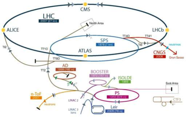
Figure 3.1: The schematic illustration of the Large Hadron Collider and its major components.

3.2   A Large Ion Collider Experiment

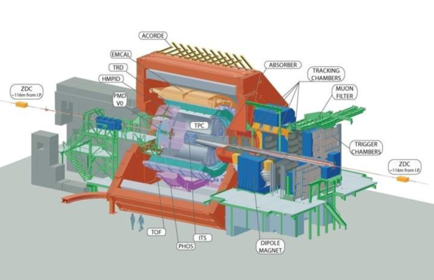
Figure 3.2: The ALICE detectors.

A Large Ion Collider Experiment (ALICE) [32] is a large multi-purpose experiment located at one of the collision points (P2) of the LHC. The ALICE collaboration involves about a thousand scientists and engineers from more than 100 institutes around the world. It has built and operates a dedicated heavy-ion detector to exploit the unique physics potential of nucleus-nucleus interactions at LHC energies. The aim is to study the physics of strongly interacting matter at extreme energy densities, where the formation of a new phase of matter, the quark-gluon plasma, is expected. The existence of such a phase and its properties are key issues in QCD for the understanding of confinement and of chiral-symmetry restoration.

ALICE has an efficient and robust tracking system that enables the detection of particles over a large momentum range, from tens of MeV/c (soft physics) to over 100 GeV/c (jet physics). A specificity of the ALICE detector relative to other LHC experiments is its large focus on particle identification (PID). PID is achieved over a large momentum range based on a variety of techniques, including specific ionization energy loss dE/dx, time-of-flight, transition and Cherenkov radiation, electromagnetic calorimetry, muon filters, and topological decay reconstruction.

This work utilizes the TPC and ITS for charged hadron reconstruction. PID is achieved with signals from the TPC and TOF detectors, while triggering and event classification is largely based on signals from the V0 detectors. A brief overview of these detectors is provided in the following paragraphs, but a more complete and detailed description of these devises and their performances are provided in [33]. The geometry and position of the detectors are illustrated in Figure 3.2.

3.2.1   ITS

The Inner Tracking System (ITS) consists of six cylindrical layers of silicon detectors for precision tracking in the pseudorapidity range $|\eta|<0.9$. The layers surround the collision point and measure the properties of particles emerging from the collision, pin-pointing their positions to a fraction of a millimeter. More details about the design, construction, calibration, and performance of the ITS can be found in [34, 33].

3.2.2   TPC

The ALICE Time Projection Chamber (TPC) is the main detector used for the detection man momentum determination of charged particles. The ALICE TPC is a conventional but large TPC optimized for extreme track densities. The design, operation, and performance of the TPC are reported in [35].

3.2.3   TOF

The ALICE Time-Of-Flight (TOF) detector consists of is a large area array of Multigap Resistive Plate Chambers (MRPC), positioned at 370-399 cm from the beam axis. It covers the full azimuth and the pseudorapidity range $|\eta|<0.9$. The TOF can separate $\pi/K$ and K/p up to approximately 2.5 GeV/c. The performance of the ALICE TOF is described in [36].

CHAPTER 4   Analysis Methods

This chapter describes the analysis methods and techniques used in the determination of the balance functions presented in this work. The analyzed datasets are described in Sec. 4.1 while the specific techniques used in this analysis are detailed in Secs. 4.2 – 4.10. Section 4.2 discusses event and track selection criteria used for inclusion of events and tracks in the determination of the correlation functions and balance functions. Section 4.4 presents a summary of the particle identification techniques used towards the identification of charged pions and kaons as well as protons and anti-protons. Section 4.6 discusses techniques and issues associated with track reconstruction and efficiency losses, whereas Sec. 4.7 elaborates on potential issues associated with splitting and merging in the reconstruction of long or close-by tracks. The roles and impacts of $\phi$-meson and $\Lambda$-baryon decays are discussed in Secs. 4.8 and 4.9, respectively. Section 4.10 presents a comparative analysis of balance functions obtained with alternative track selection criteria.

4.1   Data Samples

4.1.1   Real Data Samples

The results reported in this dissertation are based on Pb–Pb collisions at $\sqrt{s_{\mathrm{NN}}}=$ 2.76 TeV acquired during the 2010 LHC run. The analysis is specifically based on the data production LHC10h-pass2-AOD160, and involves runs taken with the ALICE magnet operated with positive and negative polarity. The data sample for this analysis is composed of the following list of runs.

Selected positive polarity runs are:
139510, 139507, 139505, 139503, 139465, 139438, 139437, 139360, 139329, 139328, 139314, 139310, 139309, 139173, 139107, 139105, 139038, 139037, 139036, 139029, 139028, 138872, 138871, 138870, 138837, 138732, 138730, 138666, 138662, 138653, 138652, 138638, 138624, 138621, 138583, 138582, 138579, 138578, 138534, 138469, 138442, 138439, 138438, 138396, 138364,

while negative polarity runs are:
138275, 138225, 138201, 138197, 138192, 138190, 137848, 137844, 137752, 137751, 137724, 137722, 137718, 137704, 137693, 137692, 137691, 137686, 137685, 137639, 137638, 137608, 137595, 137549, 137546, 137544, 137541, 137539, 137531, 137530, 137443, 137441, 137440, 137439, 137434, 137432, 137431, 137430, 137366, 137243, 137236, 137235, 137232, 137231, 137230, 137162, 137161, 137135.

These data are acquired with a minimum bias trigger based on the V0 detector and the SPD detector. A description of the triggering system and its performance are recorded in [37].

4.1.2   Monte Carlo Data Samples

In this work, we also utilize Monte Carlo (MC) simulation data of the Alice detector performance, specifically the production LHC11a10a-bis-AOD162 with option “PIDResponseTuneOnData”, which anchors the real data production LHC10h-pass2-AOD160 in Pb–Pb collisions at $\sqrt{s_{\mathrm{NN}}}=$ 2.76 TeV. The MC production LHC11a10a-bis-AOD162 is produced with the HIJING model [38], with the same run numbers as in the real data production LHC10h-pass2-AOD160.

The MC data is analyzed to determine particle identification purities reported in Sec. 4.4, and the MC closure tests reported in Sec. 4.6.4.

4.2   Event and Track Selection

This section presents a detailed description of the analysis techniques used towards event selection, collision centrality definition and selection [39], as well as track selection.

Measurements of the correlation functions are restricted to primary charged hadrons, which are reconstructed with the ALICE ITS and TPC. Events are in general acquired with minimum bias triggers primarily based on the V0 counters and the Silicon Pixel Detector (SPD). Tracks are selected based on their length determined based on the number of reconstructed space points ($N_{\rm TPCclusters}$), as well as their longitudinal ($DCA_{z}$) and radial ($DCA_{xy}$) distance of closest approach (DCA) to the collision main vertex. In ALICE, AOD tracks have a filter-bit mask, which stores the information about whether the track satisfies standard sets of quality criteria. Each filter-bit corresponds to a given set of cuts. In this work, the nominal analysis is performed on TPC only tracks corresponding to filter-bit 1.

Kinematic ranges and selection criteria were tuned to optimize the statistics (number of tracks), quality, and more specifically the purity of particle identification. Studies performed towards such optimizations are presented in Sec. 4.6.3. The data taking conditions can be summarized as follows:

• Pb–Pb collisions at $\sqrt{s_{\mathrm{NN}}}=$ 2.76 TeV

  • Accepted events: $1\times 10^{7}$ collisions,

  • Trigger: AliVEvent::kMB,

  • Centrality selection: V0-M detector,

  • Longitudinal event vertex position: $|V_{z}|\leq 6$ cm,

  • Track selection criteria (for inclusion in this analysis),

    • Charged Pion $\pi^{\pm}$

      • Transverse momentum: $0.2\leq p_{\rm T}\leq 2.0$ GeV/$c$,

      • Rapidity: $|y|\leq 0.8$ for $\pi\pi$ pair; $|y|\leq 0.7$ for cross-species pairs,

      • $N_{\rm TPCclusters}\geq 70$ out of a maximum of 159,

      • DCA: $DCA_{z}\leq 2.0$ cm, $DCA_{xy}\leq 0.04$ cm,

    • Charged Kaon $K^{\pm}$

      • Transverse Momentum: $0.2\leq p_{\rm T}\leq 2.0$ GeV/$c$,

      • Rapidity: $|y|\leq 0.7$,

      • $N_{\rm TPCclusters}\geq 70$ out of a maximum of 159,

      • DCA: $DCA_{z}\leq 2.0$ cm, $DCA_{xy}\leq 2.0$ cm,

    • (Anti-)Proton $p/\bar{p}$

      • Transverse Momentum: $0.5\leq p_{\rm T}\leq 2.5$ GeV/$c$,

      • Rapidity: $|y|\leq 0.6$ for $pp$ pair; $|y|\leq 0.7$ for cross-species pairs,

      • $N_{\rm TPCclusters}\geq 70$ out of a maximum of 159,

      • DCA: $DCA_{z}\leq 2.0$ cm, $DCA_{xy}\leq 0.04$ cm,

4.3   Analysis Software

This analysis is conducted within the context of the Physics Working Group of Correlation Function (PWG–CF) in the ALICE Collaboration, with the computing software initially developed by C. Pruneau and P. Pujahari for the study of unidentified hadron number and $p_{\rm T}$ correlations. I have further developed and generalized the code to extend the analysis to identified particle pairs with the freedom of choosing reference and associate particle species separately.

The open source analysis codes are available on Github:
https://github.com/alisw/AliPhysics/blob/master/PWGCF/Correlations/DPhi/AliAnalysisTaskGeneralBF.cxx
https://github.com/alisw/AliPhysics/blob/master/PWGCF/Correlations/DPhi/AliAnalysisTaskGeneralBF.h
https://github.com/alisw/AliPhysics/blob/master/PWGCF/Correlations/macros/PIDBFDptDpt/AddTaskGeneralBF.C

4.4   Primary Charged Hadron Identification

The identification of charged hadrons is performed using the $n\sigma$ method based on TPC dE/dx and TOF signals. Fig. 4.1 presents illustrative examples of quality assurance (QA) plots used in this work, towards the identification and separation of $\pi^{\pm}$, $K^{\pm}$, and $p/\bar{p}$. The detailed PID cuts used for the final results are listed in Fig. 4.2.

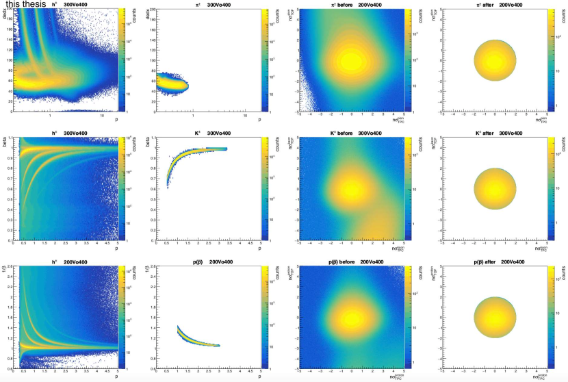
Figure 4.1: Examples of PID quality assurance plots used in this work: TPC dE/dx distribution of all charged hadrons (upper row $1^{st}$ column) and after $\pi^{\pm}$ PID cuts (upper row $2^{nd}$ column); TPC and TOF $n\sigma$ of $\pi^{\pm}$ before (upper row $3^{rd}$ column) and after PID cuts (upper row $4^{th}$ column); TOF $\beta$ distribution of all charged hadrons (middle row $1^{st}$ column) and after $K^{\pm}$ PID cuts (middle row $2^{nd}$ column); TPC and TOF $n\sigma$ of $K^{\pm}$ before (middle row $3^{rd}$ column) and after PID cuts (middle row $4^{th}$ column); TOF $1/\beta$ distribution of all charged hadrons (bottom row $1^{st}$ column) and after $p/\bar{p}$ PID cuts (bottom row $2^{nd}$ column); TPC and TOF $n\sigma$ of $p/\bar{p}$ before (bottom row $3^{rd}$ column) and after PID cuts (bottom row $4^{th}$ column).

Secondary particles are produced from weak decays and interactions of primary particles with the detector materials. Their contributions to the measured BFs reported in this work must be eliminated or at the very least suppressed. This is achieved with the use of a tight $DCA_{xy}$ cut ( $DCA_{xy}\leq 0.04$ cm ) for $\pi^{\pm}$ and $p/\bar{p}$ to remove secondary charged pions and protons. A wider $DCA_{xy}$ cut ( $DCA_{xy}\leq 2$ cm ) is applied for $K^{\pm}$, since there are fewer secondary tracks for $K^{\pm}$. Figures 4.2 and 4.3 show that after the DCA cuts are applied, the fraction of secondary particles remaining in the $\pi^{\pm}$ sample is about 1.4%, while in the $K^{\pm}$ and $p/\bar{p}$ samples, they are about 0.2%, and 5%, respectively.

The purity and contamination level of $\pi^{\pm}$, $K^{\pm}$ and $p/\bar{p}$ are plotted as a function of $p_{\rm T}$ in Fig. 4.3. The PIDResponseTuneOnData option in MC is used given it provides good dE/dx and TOF response simulations tuned to actual data. It thus provides reliable estimates of the purity of identified charged hadrons. The purities and contamination contributions from different sources are presented in Fig. 4.2. In summary, the purities of primary $\pi^{\pm}$, $K^{\pm}$ and $p/\bar{p}$ obtained in the determination of the balance functions reported in this work (i.e., final results) are about 97%, 95%, and 94%, respectively. The effects of remaining contamination are studied with various PID and DCA cuts, and used to estimate systematic uncertainties.

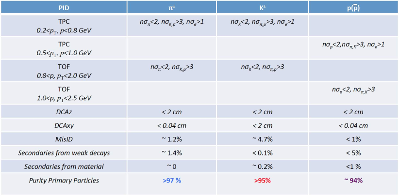
Figure 4.2: Detailed PID $n\sigma$ selection and veto cuts in TPC and TOF regions used towards the identification of $\pi^{\pm}$ ($2^{nd}$ column), $K^{\pm}$ ($3^{rd}$ column) and $p/\bar{p}$ ($4^{th}$ column), along with the DCA cuts used to reduce secondary particles from weak decays and interaction of primary particles with detector materials. The purities of identified primary hadrons along with detailed contamination percentages from different sources are also listed.

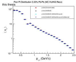
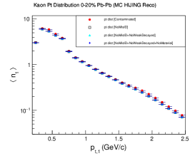
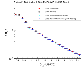
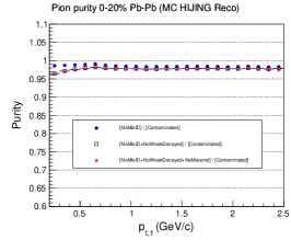
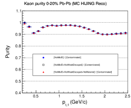
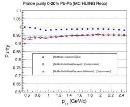
Figure 4.3: Purities (bottom row) of primary $\pi^{\pm}$ ($1^{st}$ column), $K^{\pm}$ ($2^{nd}$ column) and $p/\bar{p}$ ($3^{rd}$ column), obtained using MC reconstructed data simulations of 0-20% Pb–Pb collisions. The $p_{\rm T}$ distributions (upper row) quantify the contributions from primary particles, secondary particles from weak decays and interactions with detector materials, and mis-identified particles. Purities have similar values in other centrality ranges.

4.5   Photon Conversion Study

Photon conversions in the beam pipe and inner layers of the ALICE detector yields $e^{+}+e^{-}$ pairs ($\gamma+X\rightarrow e^{+}+e^{-}$). Electrons may be mis-identified as pions and kaons, and thus constitute a potential source of contamination in the study of the balance functions reported in this work. Additionally, given $e^{+}+e^{-}$ pairs resulting from photon conversions are emitted at small relative angles, such pairs may actually explicitly bias the $R_{2}^{US}$ correlation functions measured in this work. Such pairs would lead to a sharp and narrow spike at the origin of $R_{2}^{CD}$ correlation functions (as well as BFs). Suppressing $e^{+}+e^{-}$ pairs contamination is thus essential.

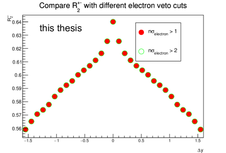
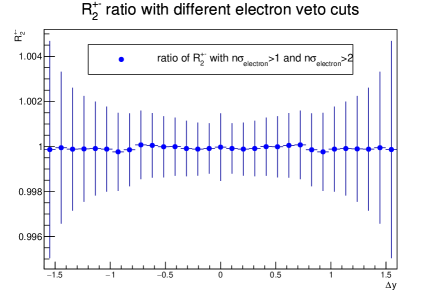
Figure 4.4: Study of the impact of photon conversions on correlation functions measured in Pb-Pb collisions: (left) Comparison of $R_{2}^{+-}$($\Delta$y) correlation functions obtained with and without an electron veto cut. (right) Ratio of the projections shown on the left. Note: Vertical bars correpond to statistical uncertainties not corrected for correlation between the $n\sigma_{electron}<1$ and $n\sigma_{electron}<2$ datasets.

Particles are rejected if within 1$\sigma$ of the electron band in the TPC dE/dx region. In the TOF region, no electron rejection cut is used for the sake of saving statistics since the electron band and the pion band overlap in the TOF $\beta$ vs momentum distribution, as shown in Fig. 4.1. Figure 4.4 displays a comparison of $R_{\pi\pi}^{+-}$($\Delta$y) obtained with electron veto cuts $n\sigma_{electron}<1$ and $n\sigma_{electron}<2$ in 20-30% Pb-Pb collisions. The two projections are nearly indistinguishable. Photon conversions thus appear to yield a very small contamination when a $n\sigma_{electron}<1$ cut is used. This less restrictive cut is thus used to minimize false rejections of pions and kaons.

4.6   Efficiency Corrections

4.6.1   Basic Issue

The correlation function $R_{2}$ is, by construction, robust against particle losses if the track detection efficiency is invariant across the experimental acceptance and independent of event parameters or detector conditions. Unfortunately, such dependences are observed in practice: The detection efficiency is a rather complicated function of the transverse momentum, the rapidity, and the azimuthal angle of the particles. It changes with detector occupancy and the position of the event primary-vertex. This work thus uses a weight technique, described in [40], to correct for such dependences.

4.6.2   Weight Correction Method and Algorithm

We describe the computation of the weights used in the study of correlation functions involving $\pi^{\pm}$ as an example. Weight calculations for other species are handled in a similar fashion. The efficiency correction weights $w^{\pm}(y,\varphi,p_{\rm T},V_{z})$ are computed using 24 bins in the primary vertex range $|V_{z}|\leq 6$ cm, 18 bins in the particle $p_{\rm T}$ range $0.2\leq p_{\rm T}\leq 2.0$ GeV, 28 bins in the azimuth range $0\leq\varphi\leq 2\pi$, and 16 bins in the rapidity range $|y|\leq 0.8$. This fine binning choice enables corrections for the efficiency dependence in 4 dimensions. The procedure used to establish the weights is as follows:

We first measure the uncorrected average transverse momentum yield, $N^{\pm}_{\rm avg}(p_{\rm T})$, of the positive and negative tracks separately. This average, though not corrected for detection efficiency, is used as the reference yield vs $p_{\rm T}$. We next measure the positive and negative track yields, $N^{\pm}_{\rm avg}(y,\varphi,p_{\rm T},V_{z})$, as a function of rapidity, y, azimuth angle, $\varphi$, and transverse momentum, $p_{\rm T}$, and the vertex position index, $V_{z}$, of the events.

The weights are thus calculated according to

$$w^{\pm}(y,\varphi,p_{\rm T},V_{z})=\frac{N^{\pm}_{\rm avg}(p_{\rm T})}{N^{\pm}(y,\varphi,p_{\rm T},V_{z})}$$ (4.1)

The full dataset is then reprocessed using these weights. Single particle and two-particle yield histograms are incremented by $w^{\pm}(y^{\alpha},\varphi^{\alpha},p_{\rm T}^{\alpha},V_{z}^{\alpha})$ and
$w^{\pm}(y^{\alpha},\varphi^{\alpha},p_{\rm T}^{\alpha},V_{z})\cdot w^{\pm}(y^{\beta},\varphi^{\beta},p_{\rm T}^{\beta},V_{z}^{\beta})$ respectively. It is verified that the use of the weights produces flat distributions in $y$, $\varphi$, and $V_{z}$.

4.6.3   Optimization of $y$ and $V_{z}$ Ranges

The LHC produces Pb–Pb collisions within a wide interaction diamond. In ALICE, the position of interaction is characterized in terms of a primary vertex position $(V_{x},V_{y},V_{z})$, where $V_{z}$ represents the longitudinal position of the interaction, i.e. the position of the vertex in the beam direction. While $V_{x}$ and $V_{y}$ represent the vertex position in the plane transverse to the beam axis. The distributions of $V_{x}$ and $V_{y}$ are typically relatively narrow and fully accepted in this analysis. The $V_{z}$ distribution, on the other hand, is rather wide, and characterized by an approximately Gaussian distribution with a standard deviation of the order of 10 cm. In the interest of maximizing the size of the statistical sample, one would wish to maximize the range of $V_{z}$-vertex position used in the analysis. However, the detector design provides for particle detection and identification optimization for collisions taking place near the nominal center of the detector. The rapidity acceptance and particle detection/identification efficiency, in particular, are found to depend on the $V_{z}$-vertex position, as schematically illustrated in Fig. 4.5. While such dependence may be partly corrected with the weight technique used in this analysis, we found that the PID acceptance becomes severely compromised for very large $|V_{z}|$ values. We thus conducted an optimization study to determine what $V_{z}$ and $y$ ranges would produce the most reliable and robust correlation functions.

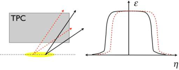
Figure 4.5: Schematic illustration of the TPC acceptance (left) and the longitudinal dependence (right) of the particle reconstruction efficiency on the vertex position $V_{z}$.

The previously published ALICE BF [28, 29] and $R_{2}^{CD}$ [3] papers reporting results on CFs of unidentified hadrons used the $|V_{z}|<10$ cm range. However, Fig. 4.6 demonstrates that the use of large $V_{z}$ ranges could cause a little ridge structure along $\Delta y=0$ in 2D $R_{2}$ correlation functions for most central events, due to the effect illustrated in Fig. 4.5. This little ridge is a charge independent effect and is present in both US and LS correlation functions with approximately the same strength. It nearly cancels out in the calculation of CD combination of correlation functions. Thus, $|V_{z}|<6$ cm is used in the final result. For most central events of $\pi\pi$ and $KK$, the remaining little ridge is also corrected for US and LS correlation functions by taking the difference between $\Delta y=0$ bins and neighbor bins. This correction is just for showing correct US and LS correlation functions, and has no impact on BFs.

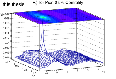
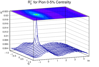
Figure 4.6: Comparison of correlation functions $R_{\pi\pi}^{+-}(\Delta y,\Delta\varphi)$ obtained with ranges $|V_{z}|<6$ cm (left) and $|V_{z}|<8$ cm (right) measured in 0-5% Pb–Pb collisions with ++ B-Field.

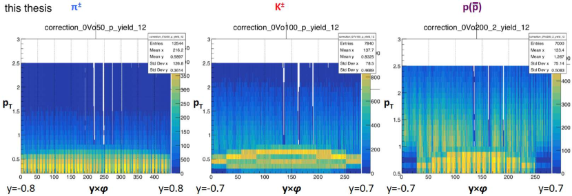
Figure 4.7: Uncorrected single-particle yield distributions of (left) $\pi^{\pm}$, (middle) $K^{\pm}$, and (right) $p/\bar{p}$, plotted as a function of rapidity $y$, azimuth $\varphi$, and $p_{\rm T}$, obtained with $0<V_{z}<0.5$ cm in central Pb–Pb collisions, measured with the ++ B-field setting.

Correlation functions of unidentified charged hadron, $R_{2}^{CD}$, previously reported by the ALICE collaboration [3], were obtained within the pseudorapidity range $|\eta|<1.0$. However, for the determination of correlation functions of identified $\pi^{\pm}$, $K^{\pm}$ and $p/\bar{p}$, reported in this work, it was necessary to narrow the the rapidity $y$ considered in order to avoid biases caused by kinematic bins featuring very small statistics (i.e., very few charged particle track entries). Figure 4.7 shows that for the $p_{\rm T}$ ranges of interest in this work, rapidity ranges must be limited to $|y|\leq 0.8$, $|y|\leq 0.7$ and $|y|\leq 0.7$ for single $\pi^{\pm}$, $K^{\pm}$ and $p/\bar{p}$, respectively.

4.6.4   MC Closure Tests

MC closure tests of $\pi\pi$ and $KK$ correlation functions (CFs) were performed to examine the robustness of the analysis procedure used in this work. The closure tests are performed for CFs of US and LS, and BFs separately, based on the MC events described in Sec. 4.1.2. Similar to real data, the analysis of simulated data is performed separately for $++$ and $--$ magnetic polarity runs to account for known differences in the detection efficiency achieved with these two magnetic field configurations. The final CF results are the weighted average of $++$ and $--$ magnetic polarity results. The same event and track selection cuts as those used with real data are employed in the closure tests. The correlators $A^{US}$ and $A^{LS}$ are first calculated at generator level separately. Primary physics tracks are used as MC Truth towards the computation of generator level correlators. They are next computed with simulated reconstructed data obtained with MC events processed with GEANT 3.0 and the ALICE detector simulation software. Weights used to construct the MC correlators are calculated using the same method and software used for real data. The closure tests are considered successful if the (simulated) reconstructed correlators match the generator level correlators with reasonable precision.

MC Closure Test of $\pi\pi$ Correlation Functions

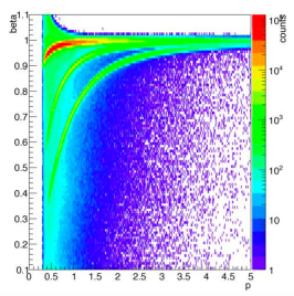
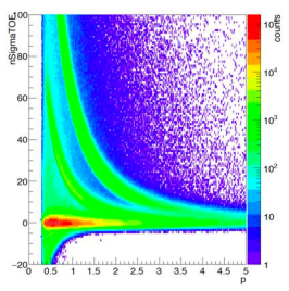
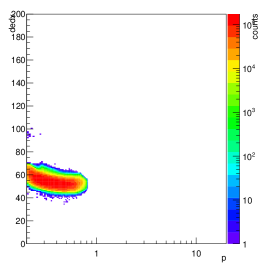
Figure 4.8: Illustration of hadron species identification based on the reconstructed level 20-40% centrality Pb–Pb MC events. Comparisons of TPC dE/dx (left column), TOF $\beta$ (middle column), and TOF $n\sigma$ (right column), as a function of momentum, before (upper row) and after (lower row) $\pi^{\pm}$ selection cuts.

For $\pi\pi$ pair, given the limited size of the MC data sample, wider centrality bins corresponding to 0-20%, 20-40%, 40-60%, and 60-80% of the interaction cross section are used. Figure 4.8 shows that the reconstructed level PID plots obtained with MC simulations are similar to those obtained with real data.

Figures 4.9 and 4.10 show that the generator and reconstructed two-dimensional US and LS correlators are similar. The reconstructed $\Delta y$ and $\Delta\varphi$ projections are about 0.5-2% (for different centralities) lower than the generator results. On one hand, this may be explained in part by pair loss in the reconstructed MC data, that are larger in central than peripheral events. On the other hand, this also could be due to the existence of about 3% mis-identified and secondary $\pi^{\pm}$ in the reconstructed $\pi^{\pm}$ sample, as shown in Fig. 4.2. The effects are present in CFs of both US and LS with approximately the same strength, thus cancels in the BF.

Figure 4.11 presents a comparison between the generator and reconstructed 2D BFs. The two BFs are found to be very similar, despite the fact that there are large fluctuations in reconstructed results due to low statistics. The differences between the reconstructed and generator projections (onto both $\Delta y$ and $\Delta\varphi$) are within two standard deviation of statistical uncertainties for almost all points.

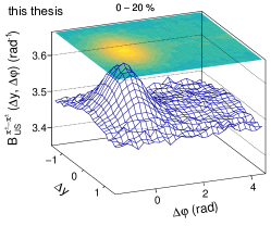
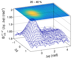
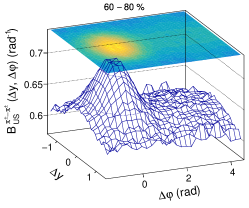
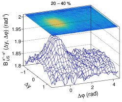
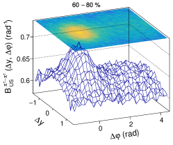
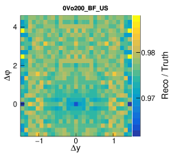
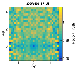
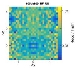
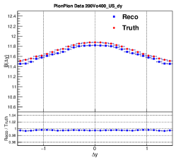
Figure 4.9: MC closure test of $\pi\pi$ pair. Comparisons of 2D CFs of US obtained with MC truth ($1^{st}$ row) and reconstructed ($2^{nd}$ row) events for selected collision centralities, and their ratios ($3^{rd}$ row). $4^{th}$ and $5^{th}$ rows: comparisons of the $\Delta y$ and $\Delta\varphi$ projections, respectively.

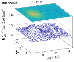
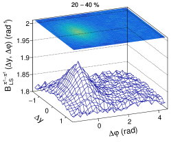
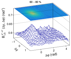
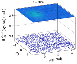
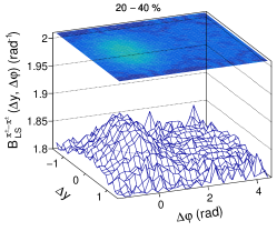
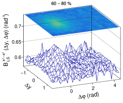
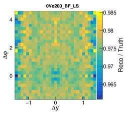
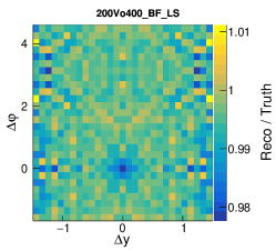
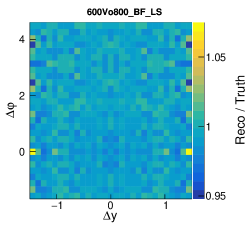
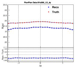
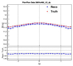
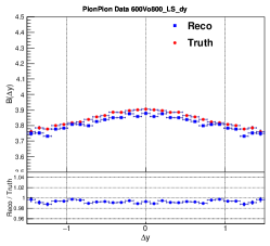
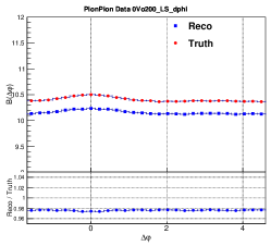
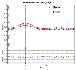
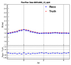
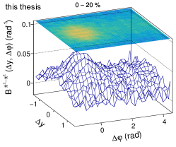
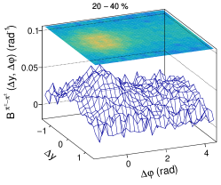
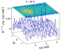
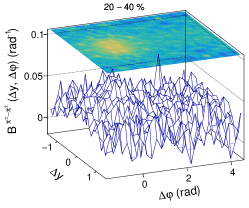
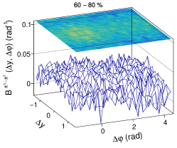
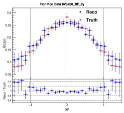
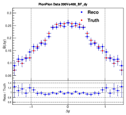
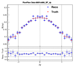
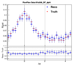
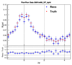
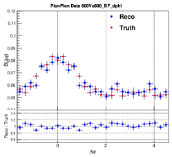
Figure 4.10: MC closure test of $\pi\pi$ pair. Comparisons of 2D CFs of LS obtained with MC truth ($1^{st}$ row) and reconstructed ($2^{nd}$ row) events for selected collision centralities, and their ratios ($3^{rd}$ row). $4^{th}$ and $5^{th}$ rows: comparisons of the $\Delta y$ and $\Delta\varphi$ projections, respectively.

Figure 4.11: MC closure test of $\pi\pi$ pair. Comparisons on 2D BFs between MC truth ($1^{st}$ row) and reconstructed ($2^{nd}$ row) results for different centralities, along with their $\Delta y$ ($3^{rd}$ row) and $\Delta\varphi$ ($4^{th}$ row) projections. The $\Delta\varphi$ projections are taken for range $|\Delta y|\leq 0.9$ to avoid large fluctuations at large $\Delta y$.

MC Closure Test of $KK$ Correlation Functions

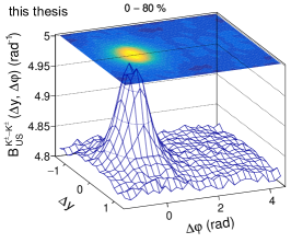
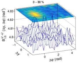
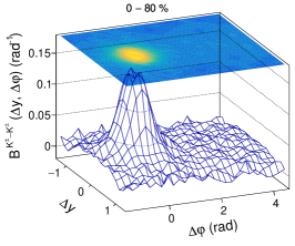
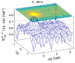
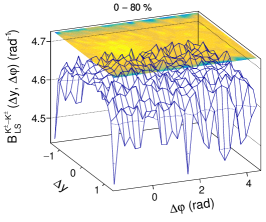
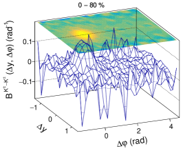
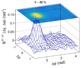
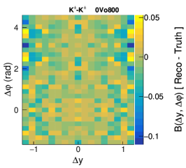
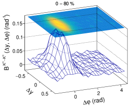
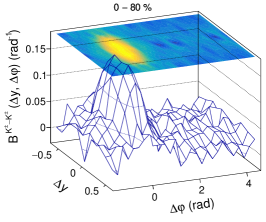
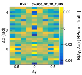
Figure 4.12: MC closure test of $KK$ pair for 0-80% centrality. $1^{st}$ row for Truth (generator level) with $|\Delta y|\leq 1.4$: US (left) and LS (middle) CFs, and BF (right). $2^{nd}$ row for $R_{\rm pure}$ (reconstructed without mis-identified and secondaries from weak decays and detector material) with $|\Delta y|\leq 1.4$: US (left) and LS (middle) CFs, and BF (right). $3^{rd}$ row for BF with $|\Delta y|\leq 1.2$: Truth (left), $R_{\rm pure}$ (middle), and their difference (right). $4^{th}$ row for BF with $|\Delta y|\leq 0.6$: Truth (left), $R_{\rm pure}$ (middle), and their difference (right).

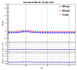
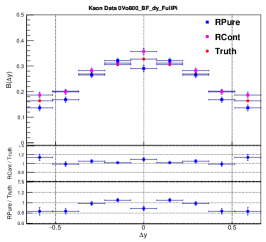
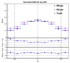
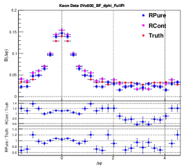
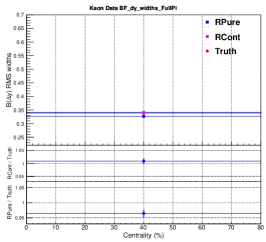
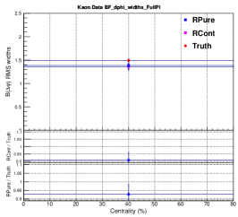
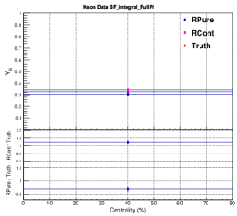
Figure 4.13: MC closure test of $KK$ pair for 0-80% centrality. Comparisons between Truth (generator level), $R_{\rm pure}$ (reconstructed without mis-identified and secondaries from weak decays and detector material), and $R_{\rm cont}$ (reconstructed with mis-identified and secondaries) with $|\Delta y|\leq 0.6$. $1^{st}$ row for CF projections: US $\Delta y$ projections for $|\Delta\varphi|\leq\pi$ (left), and US (middle) and LS (right) $\Delta\varphi$ projections. $2^{nd}$ row for BF projections: $\Delta y$ projections for $|\Delta\varphi|\leq\pi$ (left), $\Delta y$ projections for $|\Delta\varphi|\leq\pi/2$ (middle), and $\Delta\varphi$ projections (right). $3^{rd}$ row for BF with $|\Delta\varphi|\leq\pi$: $\Delta y$ widths (left), $\Delta\varphi$ widths (middle), and integrals (right). $4^{th}$ row for BF with $|\Delta\varphi|\leq\pi/2$: $\Delta y$ widths (left), $\Delta\varphi$ widths (middle), and integrals (right).

The MC closure test of $B^{KK}$ suffers from low statistics. Even MC Truth (generator level) CF of LS for 0-80% centrality do not provide a clean signal, especially for large $\Delta y$, as shown in Figure 4.12. And it is worth to mention that Gonzalez et al. has shown that large centrality bin width does not bias the $R_{2}^{CD}$ correlator [41]. Thus, reasonable MC closure test could only be accomplished for $B^{KK}$ within a large centrality bin (0-80%) and narrow relative rapidity range ($|\Delta y|\leq 0.6$), as shown in Figures 4.12,  4.13. A few % of differences on $B^{KK}$ projections, widths and integrals between MC Truth (generator level), $R_{\rm pure}$ (reconstructed without mis-identified and secondaries from weak decays and detector material), and $R_{\rm cont}$ (reconstructed with mis-identified and secondaries) are consistent with expected systematics and low statistics.

The $B^{\pi\pi}$ and $B^{KK}$ results show that the MC closure tests are successful. We conclude that the data analysis techniques used in this analysis are sufficiently robust for measuring BFs of charged hadron pairs $(\pi,K,p)\otimes(\pi,K,p)$.

4.6.5   Additional $p_{\rm T}$-dependent Efficiency Correction

We carried out an additional $p_{\rm T}$-dependent efficiency correction study to insure that the efficiency correction method applied in this work, and described in Sec. 4.6, produces robust CF results.

The use of both TPC and TOF for PID in this work results in $p_{\rm T}$-dependent detection efficiencies for $\pi^{\pm}$, $K^{\pm}$, and $p/\bar{p}$. In Figures 4.14, 4.15, 4.16, the $p_{\rm T}$-dependent efficiencies are estimated based on the ratio of HIJING MC truth and reconstructed $p_{\rm T}$ spectra obtained with full GEANT simulated Pb–Pb collisions. The MC corrected $p_{\rm T}$ spectra of real data are very similar to the ALICE published $p_{\rm T}$ spectra [8], with only a 10-15% discrepancies on average between the two, which in principle are good enough for CFs and will not bias the results. The discrepancies are due to the fact that HIJING reconstructed events could not reproduce the real data $DCA_{xy}$ distribution, as shown in Figure 4.17. Thus the MC detection efficiency estimations by HIJING reconstructed data are not robust for tight DCA cuts, which makes it difficult to perfectly reproduce the published $p_{\rm T}$ spectra.

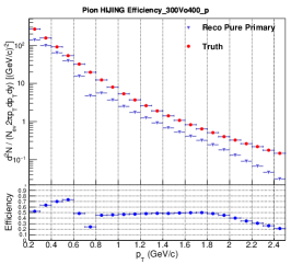
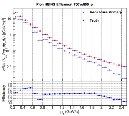
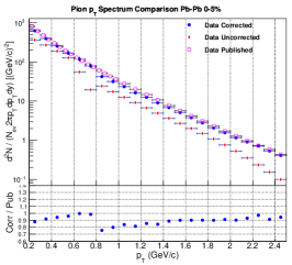
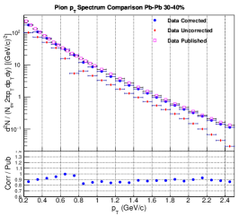
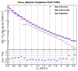
Figure 4.14: For $\pi^{\pm}$. Upper row for MC: efficiency estimation by taking the ratio of reconstructed divided by generator $p_{\rm T}$ spectra. Lower row for real data: comparison of $p_{\rm T}$ spectra obtained with and without MC efficiency correction, and the ALICE published, in central (left), mid-central (middle) and peripheral (right) collisions.

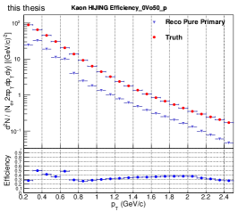
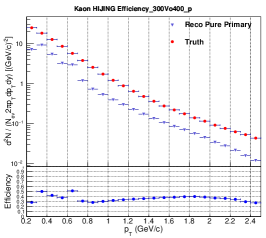
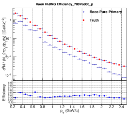
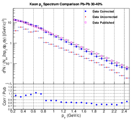
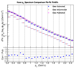
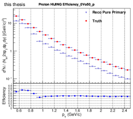
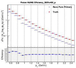
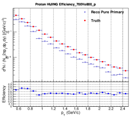
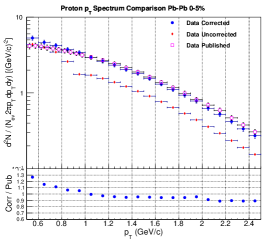
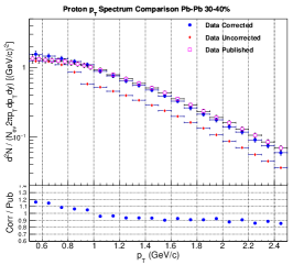
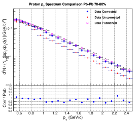
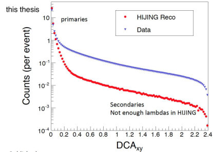
Figure 4.15: For $K^{\pm}$. Upper row for MC: efficiency estimation by taking the ratio of reconstructed divided by generator $p_{\rm T}$ spectra. Lower row for real data: comparison of $p_{\rm T}$ spectra obtained with and without MC efficiency correction, and the ALICE published, in central (left), mid-central (middle) and peripheral (right) collisions.

Figure 4.16: For $p/\bar{p}$. Upper row for MC: efficiency estimation by taking the ratio of reconstructed divided by generator $p_{\rm T}$ spectra. Lower row for real data: comparison of $p_{\rm T}$ spectra obtained with and without MC efficiency correction, and the ALICE published, in central (left), mid-central (middle) and peripheral (right) collisions.

Figure 4.17: For $p/\bar{p}$. Comparison on $DCA_{xy}$ distributions between data and reconstructed HIJING MC in 0-20% centrality of Pb-Pb collisions.

Figures 4.18, 4.19 show three sets of $B^{pp}$ results obtained with different $p_{\rm T}$-dependent efficiency corrections. The first set is obtained without a $p_{\rm T}$-dependent efficiency correction. The second set is based on a MC $p_{\rm T}$-dependent efficiency correction, which uses the difference between the raw and the MC corrected $p_{\rm T}$ spectra as a correction factor. The third set is obtained with a data driven $p_{\rm T}$-dependent efficiency correction, which uses the difference between the raw and the published $p_{\rm T}$ spectra as a correction factor. The three sets of BF results are in good agreement with each other. Differences between the three sets of results are within 1% for $\Delta y$ widths and BF integrals, whereas the differences between $\Delta\varphi$ widths are within a few percent, although both the MC and data driven corrections tend to make the BF slightly narrower in $\Delta\varphi$. This bias may in part be explained by the fact that the MC and data driven corrections add more weight to higher $p_{\rm T}$ (TOF region) particles in the sample. High-$p_{\rm T}$ particles, particularly those produced by fragmentation of jets, are in general more likely to be emitted at smaller relative angle $\Delta\varphi$. Increasing the relative weight of the high-$p_{\rm T}$ pairs in the sample should thus produce a slight narrowing of the correlation functions and balance functions averaged over the range measured in this work. Since the “MC corrected” results lie in-between the “uncorrected” and “data driven corrected” results, we use the difference between the latter two sets to estimate systematic uncertainties associated with a $p_{\rm T}$-dependent efficiency correction.

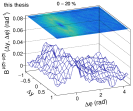
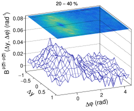
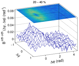
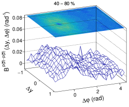
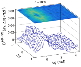
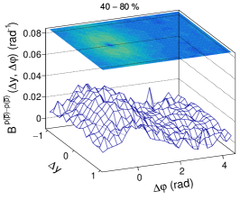
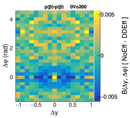
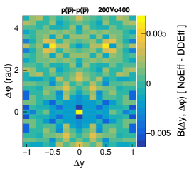
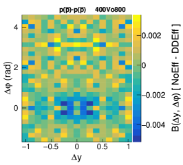
Figure 4.18: Comparison of 2D $B^{pp}$ obtained without (1st row), with MC (2nd row) and Data Driven (3rd row) efficiency correction. 4th row: differences between without and with Data Driven $p_{\rm T}$-dependent efficiency correction.

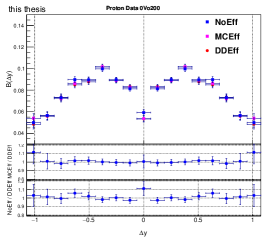
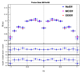
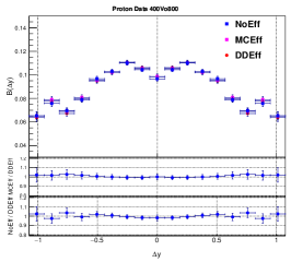
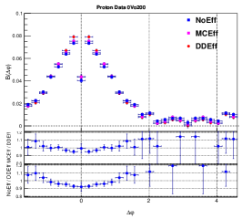
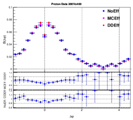
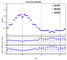
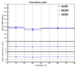
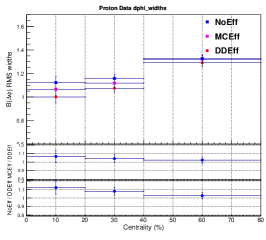
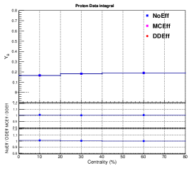
Figure 4.19: Comparisons of $B^{pp}$ $\Delta y$ projections (top row), $\Delta\varphi$ projections (middle row), and $\Delta y$ and $\Delta\varphi$ widths, and integrals (bottom row), obtained without, with MC and Data Driven $p_{\rm T}$-dependent efficiency correction. In each plot, the second pad presents the ratio of $B^{pp}$ obtained with MC and Data Driven $p_{\rm T}$-dependent efficiency correction, while the third pad exhibits the ratio of $B^{pp}$ obtained without and with Data Driven $p_{\rm T}$-dependent efficiency correction.

Figures 4.20 – 4.24 show that the “uncorrected” BF results and the “data driven” $p_{\rm T}$-dependent efficiency corrected results are in good agreement for both same- and cross-species pairs. Differences between the two sets of results are with 1$\sigma$ of statistical uncertainties at essentially all $\Delta y$ and $\Delta\varphi$ separations. In this work, we thus report “final results” for balance functions based on the “data driven” $p_{\rm T}$-dependent efficiency correction method for all species pairs. The differences between the “uncorrected” results and the “data driven corrected” results are taken as systematic uncertainty associated with this data driven $p_{\rm T}$-dependent efficiency correction.

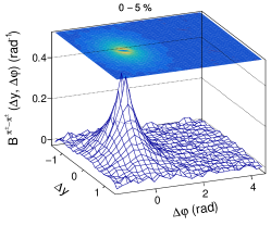
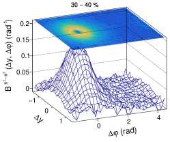
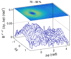
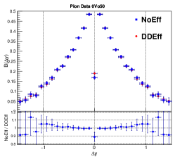
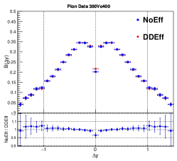
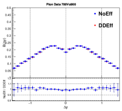
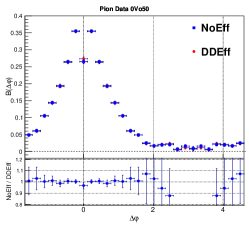
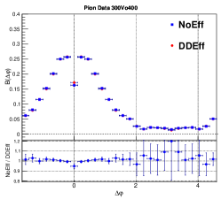
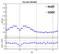
Figure 4.20: Comparisons of 2D $B^{\pi\pi}$ obtained without (1st row) and with Data Driven (2nd row) $p_{\rm T}$-dependent efficiency correction for selected centralities, along with their $\Delta y$ (3rd row) and $\Delta\varphi$ projections (4th row), $\Delta y$ and $\Delta\varphi$ widths, and integrals (5th row).

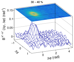
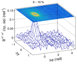
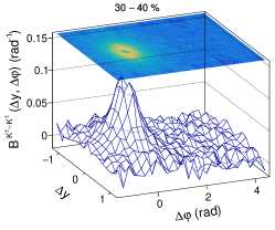
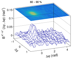
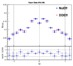
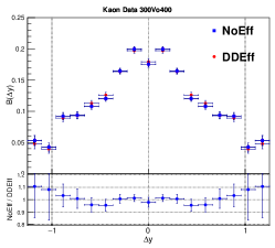
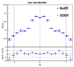
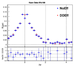
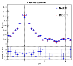
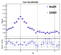
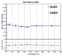
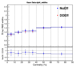
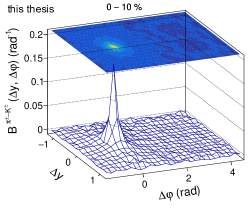
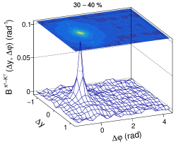
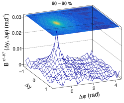
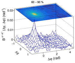
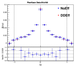
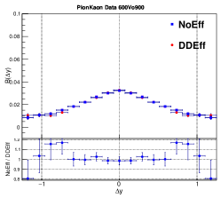
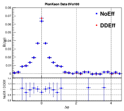
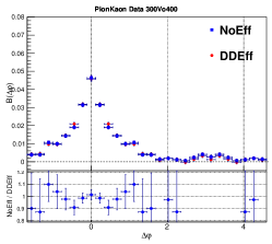
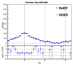
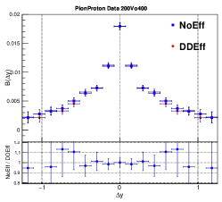
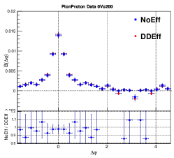
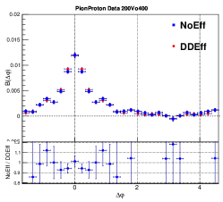
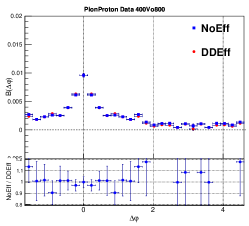
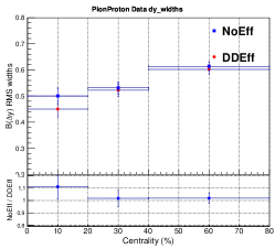
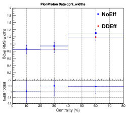
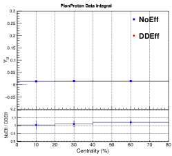
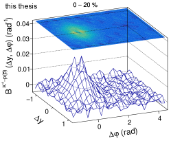
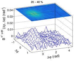
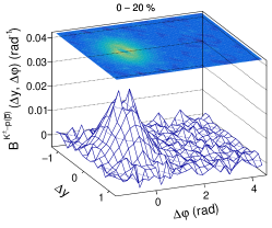
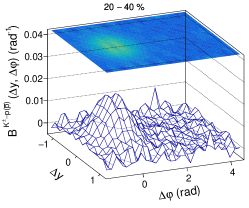
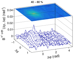
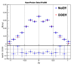
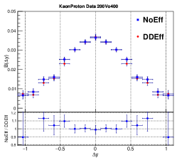
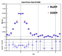
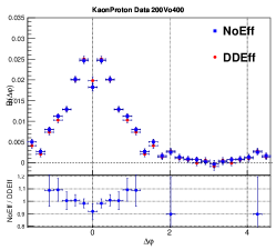
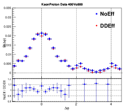
Figure 4.21: Comparisons of 2D $B^{KK}$ obtained without (1st row) and with Data Driven (2nd row) $p_{\rm T}$-dependent efficiency correction for selected centralities, along with their $\Delta y$ (3rd row) and $\Delta\varphi$ projections (4th row), $\Delta y$ and $\Delta\varphi$ widths, and integrals (5th row).

Figure 4.22: Comparisons of 2D $B^{\pi K}$ obtained without (1st row) and with Data Driven (2nd row) $p_{\rm T}$-dependent efficiency correction for selected centralities, along with their $\Delta y$ (3rd row) and $\Delta\varphi$ projections (4th row), $\Delta y$ and $\Delta\varphi$ widths, and integrals (5th row).

Figure 4.23: Comparisons of 2D $B^{\pi p}$ obtained without (1st row) and with Data Driven (2nd row) $p_{\rm T}$-dependent efficiency correction for selected centralities, along with their $\Delta y$ (3rd row) and $\Delta\varphi$ projections (4th row), $\Delta y$ and $\Delta\varphi$ widths, and integrals (5th row).

Figure 4.24: Comparisons of 2D $B^{Kp}$ obtained without (1st row) and with Data Driven (2nd row) $p_{\rm T}$-dependent efficiency correction for selected centralities, along with their $\Delta y$ (3rd row) and $\Delta\varphi$ projections (4th row), $\Delta y$ and $\Delta\varphi$ widths, and integrals (5th row).

4.7   Track Splitting Study

Track splitting occurs when the track reconstruction software fails to properly connect track segments that belong together thereby producing two reconstructed tracks instead of one. Such failures occur when hits belonging to two track segments are not properly aligned. Track splitting may thus yield a narrow spike at the origin of 2D $B_{LS}(\Delta y,\Delta\varphi)$ of same-species pairs, namely $\pi\pi$, $KK$, and $pp$ pairs.

Track splitting may nominally be suppressed by requiring all tracks included in the analysis are reconstructed with more than half of the possible number of hits they can have according to their geometry. However, imposing a “long track” requirement greatly reduces the number of accepted tracks and thus the statistical quality of the measured CFs. It is thus important not to use too stringent a cut. In this work, a cut $N_{\rm TPCclusters}\geq 70$ out of a maximum of 159 is used for selecting tracks, which in principle suppresses a majority of the split tracks. In addition, a comparison with a set of BF results with a cut $N_{\rm TPCclusters}\geq 85$ is taken as an independent systematic uncertainty, the details of which are in Chapter 5. The differences of BF results between $N_{\rm TPCclusters}\geq 70$ and $N_{\rm TPCclusters}\geq 85$ are smaller than 1%. The impact of split tracks on $R_{2}^{LS}$ correlation function reported in this work is thus expected to be essentially negligible.

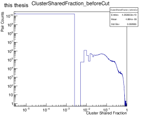
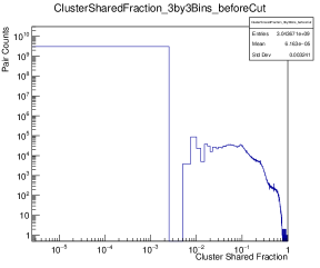
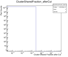
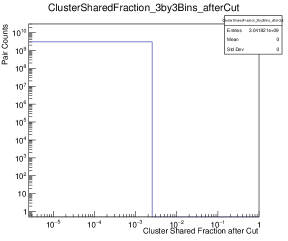
Figure 4.25: Comparison of $B_{LS}^{\pi\pi}$($\Delta y$,$\Delta\varphi$) of 0-5% centrality obtained without (top row) and with (bottom row) the TPC cluster sharing cut ($SharingFraction<0.25\%$). Left column plots are TPC cluster shared fraction in the full $\Delta y$ and $\Delta\varphi$ acceptance. Middle column plots are TPC cluster shared fraction in the 3$\times$3 bins around $\Delta y$=0,$\Delta\varphi$=0. Right column plots are the $B_{LS}^{\pi\pi}$($\Delta y$,$\Delta\varphi$) of 0-5% results.

We nonetheless further explored the possibility of split tracks by means of a study of TPC shared track fraction. The study is based on a technique borrowed from the HBT working group. We used a function named CalculateSharedFraction derived from the source code AliFemtoShareQualityPairCut.cxx, and which was extensively applied for checking the presence of TPC shared hits and split tracks in many other ALICE analyses. Figure 4.25 shows the TPC shared track fraction and compares the $B_{LS}^{\pi\pi}$($\Delta y$,$\Delta\varphi$) correlator measured in the 0-5% collision centrality before and after a strict TPC shared track fraction cut. One finds that the narrow near-side peak at ($\Delta y$=0,$\Delta\varphi$=0) is not due to the track splitting. The size difference of the near-side peak at ($\Delta y$=0,$\Delta\varphi$=0) of $B_{LS}^{\pi\pi}$($\Delta y$,$\Delta\varphi$) is used to correct the TPC cluster sharing effect. Figure 4.26 shows that the differences between TPC sharing corrected and not corrected for BF $\Delta y$ and $\Delta\varphi$ RMS widths, and integral are smaller than 1%. This TPC cluster sharing correction is included in the final BF results reported in this work. Results presented in Figs 4.27 – 4.30 show that TPC cluster sharing effects observed with $KK$ and $pp$ pairs are similar to those observed for $\pi\pi$ pair.

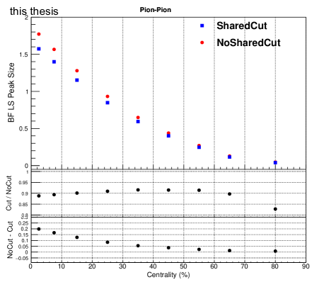
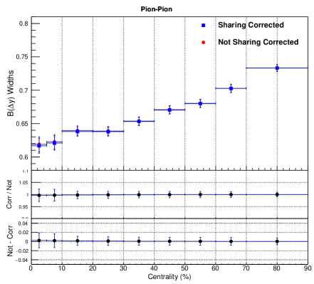
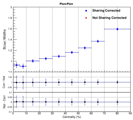
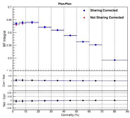
Figure 4.26: Comparison of the peak size at (0,0) bin of $B_{LS}^{\pi\pi}(\Delta y,\Delta\varphi)$ obtained with and without TPC sharing cut (upper left), which serves as a correction for $B^{\pi\pi}$. And comparison of the $B^{\pi\pi}$ $\Delta y$ RMS widths (upper right), $\Delta\varphi$ RMS widths (lower left), and integrals (lower right) obtained with and without TPC sharing correction.

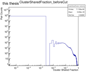
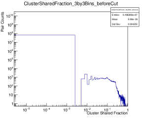
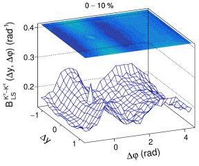
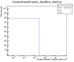
Figure 4.27: Comparison of $B_{LS}^{KK}$($\Delta y$,$\Delta\varphi$) of 0-10% centrality obtained without (top row) and with (bottom row) the TPC cluster sharing cut ($SharingFraction<0.25\%$). Left column plots are TPC cluster shared fraction in the full $\Delta y$ and $\Delta\varphi$ acceptance. Middle column plots are TPC cluster shared fraction in the 3$\times$3 bins around ($\Delta y$=0,$\Delta\varphi$=0). Right column plots are the $B_{LS}^{KK}$($\Delta y$,$\Delta\varphi$) of 0-10% results.

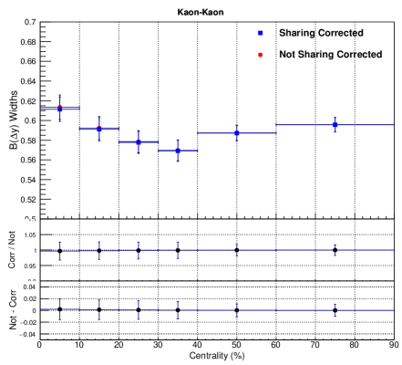
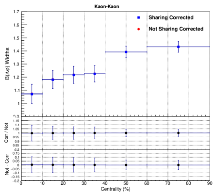
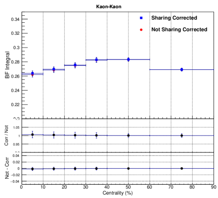
Figure 4.28: Comparison of the peak size at (0,0) bin of $B_{LS}^{KK}(\Delta y,\Delta\varphi)$ obtained with and without TPC sharing cut (upper left), which serves as a correction for $B^{KK}$. And comparison of the $B^{KK}$ $\Delta y$ RMS widths (upper right), $\Delta\varphi$ RMS widths (lower left), and integrals (lower right) obtained with and without TPC sharing correction.

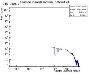
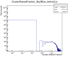
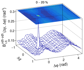
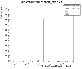
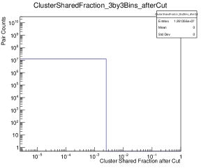
Figure 4.29: Comparison of $B_{LS}^{pp}$($\Delta y$,$\Delta\varphi$) of 0-20% centrality obtained without (top row) and with (bottom row) the TPC cluster sharing cut ($SharingFraction<0.25\%$). Left column plots are TPC cluster shared fraction in the full $\Delta y$ and $\Delta\varphi$ acceptance. Middle column plots are TPC cluster shared fraction in the 3$\times$3 bins around ($\Delta y$=0,$\Delta\varphi$=0). Right column plots are the $B_{LS}^{pp}$($\Delta y$,$\Delta\varphi$) of 0-20% results.

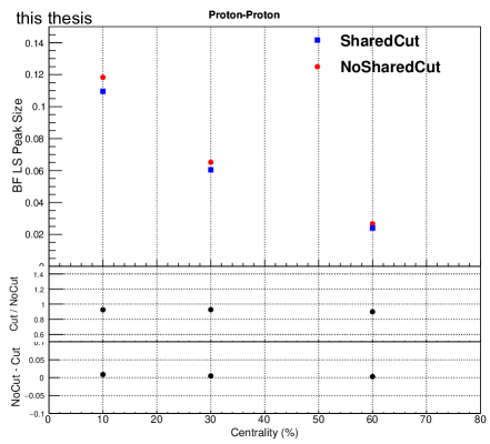
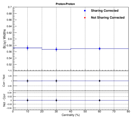
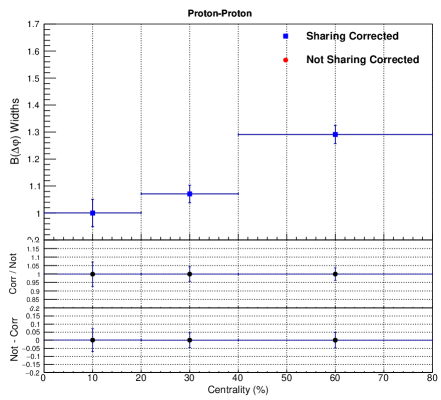
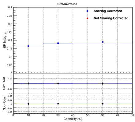
Figure 4.30: Comparison of the peak size at (0,0) bin of $B_{LS}^{pp}(\Delta y,\Delta\varphi)$ obtained with and without TPC sharing cut (upper left), which serves as a correction for $B^{pp}$. And comparison of the $B^{pp}$ $\Delta y$ RMS widths (upper right), $\Delta\varphi$ RMS widths (lower left), and integrals (lower right) obtained with and without TPC sharing correction.

4.8   $\phi$-Meson Decay in $B^{KK}$

Nuclear collisions produce a relatively small but non-negligible amount of $\phi$-mesons. These mesons have a lifetime of $1.55\pm 0.01\times 10^{-22}$ s, which is of the order of the lifespan of the fireball produced in Pb–Pb collisions. The particles $\phi$-mesons decay into, particularly pairs of $K^{+}$ and $K^{-}$ strange mesons, are thus considered primary particles in the context of this analysis. By virtue of their origin, such $K^{+}+K^{-}$ pairs are intrinsically correlated and thus expected to form observable correlation structures in $KK$ balance functions. But given these kaons are considered primary particles (they do not result from weak-interaction decays), no correction for their presence in the data sample is required. However, the production and transport properties of $\phi$-mesons may differ from those of “ordinary” kaons, i.e., those not originating from $\phi$-mesons. It is thus of interest to investigate whether the presence of $\phi$-meson decays influence the shape and evolution of $KK$ balance functions with collision centrality.

4.8.1   $\phi$-Meson Yield

We evaluated the yield of $\phi$-meson decays into $K^{+}$+$K^{-}$ pairs based on the $\phi$-meson (two charged kaons) invariant mass distributions of US and LS kaon pairs in Fig. 4.31. We found that the number of $K^{+}$+$K^{-}$ pairs from $\phi$-meson decays is smaller than 3 % of the total number of $K^{+}$+$K^{-}$ pairs observed in the near-side peak region of US correlations. However, because they tend to be emitted at small relative angle and rapidity, due in part to kinematical focusing associated with radial flow, $K^{+}$+$K^{-}$ pairs from $\phi$-meson may nonetheless contribute a sizable fraction of the near-side peak of $KK$ balance functions. We thus further explored contributions to the $KK$ BFs based on MC studies.

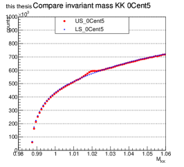
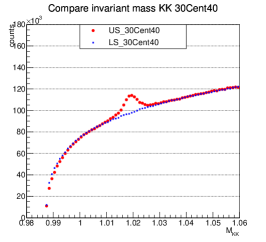
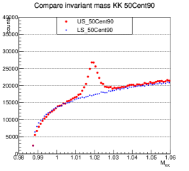
Figure 4.31: Comparison of US and LS kaon pairs invariant mass distributions obtained in (left) central , (middle) mid-central, and (right) peripheral Pb–Pb collisions.

4.8.2   MC Study of $\phi$-Meson Decay in $B^{KK}$

A MC study of $\phi$ meson decayed $K^{+}$+$K^{-}$ pair contribution in $B^{KK}$ was performed using the HIJING generator level data described in Sec. 4.1.2. Unfortunately, a similar study using simulation data produced with the AMPT model, which features more realistic $\phi$-meson yields, is not possible because the AMPT dataset produced by the ALICE collaboration does not contain information of decaying mother particles. Producing an independent AMPT dataset suitable for this study is beyond the scope and resources of this work.

Figure 4.32 presents a comparison of two-dimensional $B^{KK}$ balance functions obtained with the inclusion (top) and the exclusion (bottom) of charged kaon pairs originating from $\phi$-mesons in three ranges of Pb–Pb collision centralities. Projections of these balance functions onto the $\Delta y$ and $\Delta\varphi$ axes are displayed in Fig. 4.33. One finds that the amplitude of the near-side peak of the balance function is suppressed by about 30% when contributions from $\phi$-meson decays are explicitly excluded. Figure 4.33 further shows that $\phi$-meson decays could possibly lower the $B^{KK}$ $\Delta y$ and $\Delta\varphi$ widths by about 7-8%, and increase the integrals by about 3-4%.

The STAR Collaboration measured $B^{KK}$ in terms of $q_{inv}$ in Au–Au collisions at $\sqrt{s_{{}_{\rm NN}}}=$200 GeV in nine centrality bins [15]. They concluded that the $\phi$-meson decay contribution in $B^{KK}(q_{inv})$ is approximately 50%, independent of centrality.

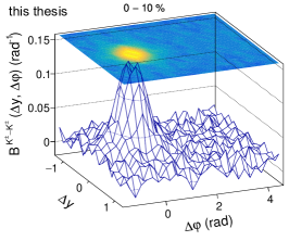
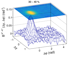
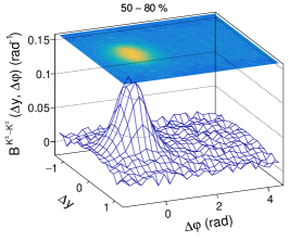
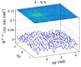
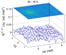
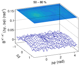
Figure 4.32: Comparison of $KK$ BFs obtained when including (top row) and excluding (bottom row) $\phi$-meson decays from MC HIJING generator level data in three selected ranges of Pb-Pb collision centralities.

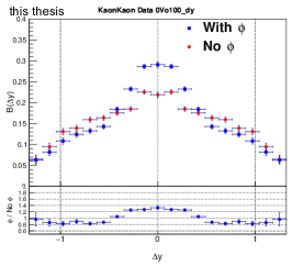
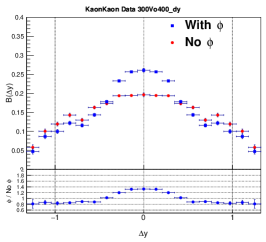
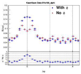
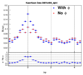
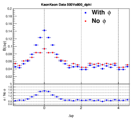
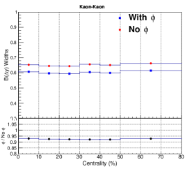
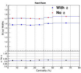
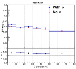
Figure 4.33: For $KK$ using MC HIJING generator level data. Comparisons on BF $\Delta y$ (top row) and $\Delta\varphi$ (middle row) projections of different centralities, and $\Delta y$ widths (lower left), $\Delta\varphi$ widths (lower middle), and BF integrals (lower right) between phi meson decay included and excluded.

4.9   Lambda Weak Decay in $B^{\pi p}$ and $B^{p\pi}$

We investigated the presence of contamination from Lambda baryon ($\Lambda$/$\bar{\Lambda}$) decays in $B^{\pi p}$ and $B^{p\pi}$ balance functions. Lambda baryon decays occur on a weak-interaction time scale of $(2.631\pm 0.020)\times 10^{-10}$ s (in their rest frame). Their daughter products, protons and pions (or anti-particles), are thus considered secondary particles in the context of this work. Secondary pions and protons (anti-protons) must thus be suppressed in measurements of $\pi\pi$, $\pi p$, and $pp$ balance functions. In this work, this was accomplished by means of tight DCA cuts. Achieved estimated purities were already discussed in Sec. 4.4. The discussion presented in this section focuses on the impact of secondary pions and protons on the $B^{\pi p}$ balance function, which is most susceptible to contamination from $\Lambda$/$\bar{\Lambda}$ decays.

4.9.1   Tight $DCA_{xy}$ Cut

The $\Lambda$/$\bar{\Lambda}$ decay daughter particles may cause feed down contamination in $B^{\pi p}$ and $B^{p\pi}$. Figures 4.34 and 4.35 show that a tight $DCA_{xy}<0.04$ cm cut does a much better job at removing the secondary particles from both weak decays and interaction of produced particles with detector materials than a wide $DCA_{xy}<2.4$ cm cut. Furthermore, in Fig. 4.36, the $\Lambda$ invariant mass plots show that the $\Lambda$ signal is better suppressed by the tight $DCA_{xy}<0.04$ cm cut than the wide $DCA_{xy}<2.4$ cm cut. Thus in this work, a tight $DCA_{xy}<0.04$ cm cut is used to reduce secondary $\pi^{\pm}$ and $p/\bar{p}$. Note that a similar tight $DCA_{xy}$ cut was also used to remove secondary particles in other published ALICE PID CF papers [42]. After this tight $DCA_{xy}<0.04$ cm cut, we estimate that only about 1.4% of $\pi^{\pm}$ and 4% of $p/\bar{p}$ are from weak decays. This should lead to only minor contamination in $B^{\pi p}$ and $B^{p\pi}$.

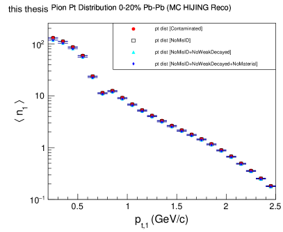
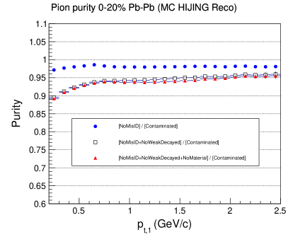
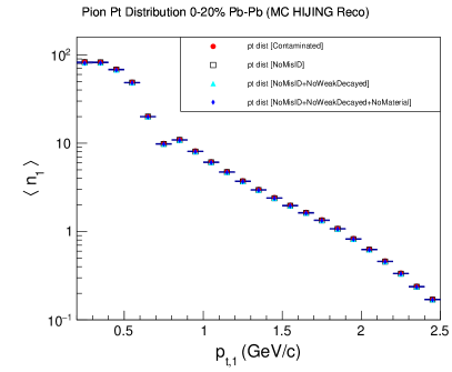
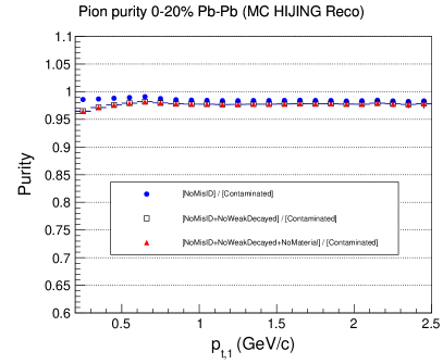
Figure 4.34: Comparison of primary $\pi^{\pm}$ purities (right column) obtained with cuts $DCA_{xy}<2.4$ cm (top row) and $DCA_{xy}<0.04$ cm (bottom row) in 0-20% centrality Pb–Pb collisions. The purities are calculated using MC reconstructed data, and are based on the $p_{\rm T}$ distributions of $\pi^{\pm}$ (left column) with contributions from primary particles, secondary particles from weak decays and interaction with detector materials, and mis-identified particles, separately. Purities have similar values for other centralities.

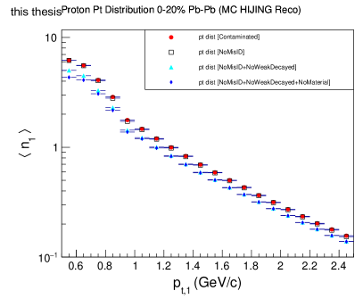
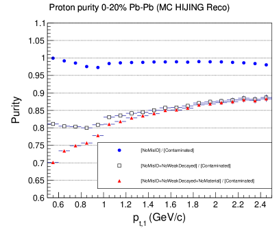
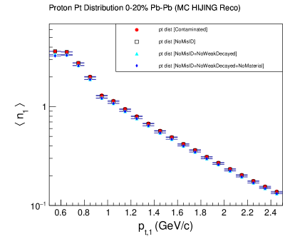
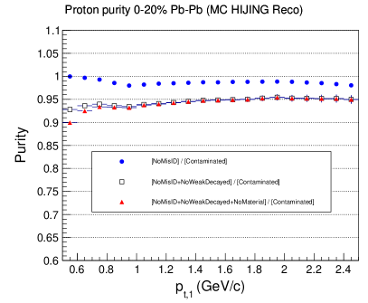
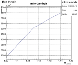
Figure 4.35: Comparison of primary $p/\bar{p}$ purities (right column) obtained with cuts $DCA_{xy}<2.4$ cm (top row) and $DCA_{xy}<0.04$ cm (bottom row) in 0-20% centrality Pb–Pb collisions. The purities are calculated using MC reconstructed data, and are based on the $p_{\rm T}$ distributions of $p/\bar{p}$ (left column) with contributions from primary particles, secondary particles from weak decays and interaction with detector materials, and mis-identified particles, separately. Purities have similar values for other centralities.

Figure 4.36: Study of the impact of $\Lambda$ weak decay contamination in measurements of $B^{\pi p}$. The $\Lambda$ invariant mass of US pairs (left column), 2D $B^{\pi p}$ (middle column), and $\Delta y$ projections (right column) obtained with cuts $DCA_{xy}<2.4$ cm (top row) and $DCA_{xy}<0.04$ cm (bottom row) in 20-40% centrality Pb–Pb collisions.

4.9.2   Lambda Invariant Mass Check

In addition, in order to make sure that contributions to $B^{\pi p}$ from $\Lambda$ decays (contamination) is negligible after a tight $DCA_{xy}<0.04$ cm cut is applied, we performed a $\Lambda$ invariant mass cut study. Figure 4.37 presents $\Delta y$ and $\Delta\varphi$ projections of $\pi p$ balance functions in three collision centrality ranges. BFs used to calculate these projections were obtained with three distinct sets of $\pi p$ pairs invariant mass criteria. The first set (labelled “With $\Lambda$”) is obtained with all $\pi p$ pairs, i.e., without selection based on the invariant mass of the pair. The second set (labelled No $\Lambda$) involves the use of a mass cut to eliminate all particle pairs with $1\sigma$ $\Lambda$ invariant mass cut ($1.114683<mInv_{\Lambda}<1.116683$). The third set involves removal of pairs with a $\Lambda$ invariant mass sideband cut ($1.1109<mInv_{\Lambda}<1.1131$). This cut is selected to remove approximately the same number of particle pairs but is off the $\Lambda$ mass peak. It is thus possible to compare balance function obtain with all pairs, pairs that exclude the $\Lambda$ mass region, and a set of pairs from which $\Lambda$ are not removed but an equivalent number of pairs is. The top and middle rows of Fig. 4.37 show projections along $\Delta y$ and $\Delta\varphi$, respectively, as well as ratios of these projections. One notes that the amplitude and shape of the three projections are nearly identical, thereby confirming that the explicit removal of pairs with a $\Lambda$ mass has a very small impact on the balance functions and their projections. Furthermore, the bottom row of the figure displays a comparison of the $\Delta y$ and $\Delta\varphi$ rms widths and the integral of the balance functions vs. the Pb–Pb collision centrality. One finds that the widths and BF integrals obtained with and without mass cuts are essentially identical. One then concludes from these comparisons that the residual contamination of $\Lambda$ decays into the $B^{\pi p}$ balance function reported in this work is essentially negligible.

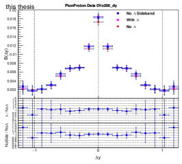
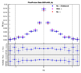
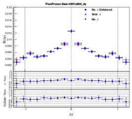
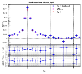
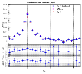
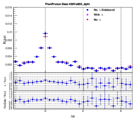
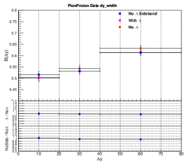
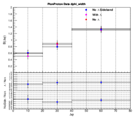
Figure 4.37: Study of the impact of $\Lambda$ weak decay contamination in measurements of $B^{\pi p}$ with the tight $DCA_{xy}<0.04$ cm cut. Comparisons on BF $\Delta y$ projections (top row), $\Delta\varphi$ projections of different centralities (middle row), and $\Delta y$ widths (lower left), $\Delta\varphi$ widths (lower middle), and BF integrals (lower right) between without and with a $1\sigma$ $\Lambda$ invariant mass cut ($1.114683<mInv_{\Lambda}<1.116683$), and with a $\Lambda$ invariant mass sideband cut ($1.1109<mInv_{\Lambda}<1.1131$). The $\Lambda$ invariant mass cut (corresponds to the blue lines in lower left plot in Fig. 4.36) and the sideband cut (corresponds to the red lines in lower left plot in Fig. 4.36) remove approximately same number of US pairs.

4.10   Study of BF with Other Filter-bits

The final BF results reported in this work are obtained with TPC only tracks corresponding to filter-bit 1, as described in Sec. 4.2. However, we have also studied BFs obtained with global tracks with tight DCA cut, corresponding to filter-bit 96.

The differences between BFs obtained with filter-bit 1 and 96, as shown in
Figures 4.38, 4.40, 4.41, 4.42, 4.43, 4.44, where most points in the projection, width and integral plots comparing BFs of filter-bit 1 and 96 are within two standard deviation of statistical uncertainties. Larger differences between BFs obtained with filter-bits 1 and 96 are observed at $\Delta y=0$ and $\Delta\varphi=0$ in the projections of $B^{\pi\pi}$, especially for most central events, as shown in Fig. 4.38. These are due to differences on CFs of LS at $\Delta y=0$ and $\Delta\varphi=0$ between filter-bit 1 and 96, as shown in Figure 4.39, which are probably because filter-bit 96 incorporates the refit towards the ITS. Thus, in the final $B^{\pi\pi}$ and $B^{pp}$ results, the differences on $(\Delta y,\Delta\varphi)=(0,0)$ bin between filter-bit 1 and 96 are taken as an additional systematic uncertainty for $(\Delta y,\Delta\varphi)=(0,0)$ bin.

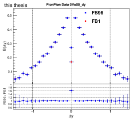
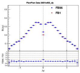
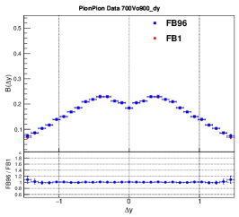
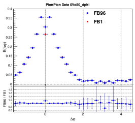
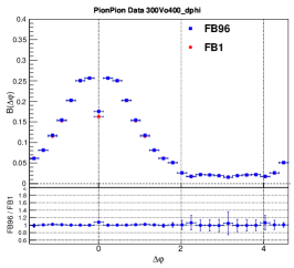
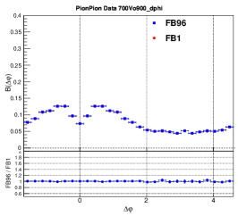
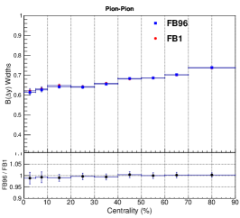
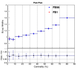
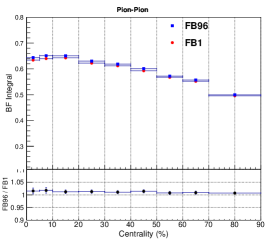
Figure 4.38: Comparisons of $B^{\pi\pi}$ projections onto $\Delta y$ (top row) and $\Delta\varphi$ (middle row) axis for selected collision centralities. Bottom row: comparisons of $B^{\pi\pi}$ $\Delta y$ widths (left), $\Delta\varphi$ widths (middle), and integrals (right) as a function of collision centrality between filter-bit 1 and 96.

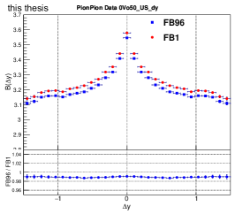
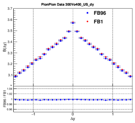
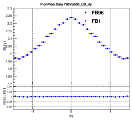
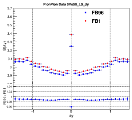
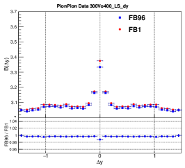
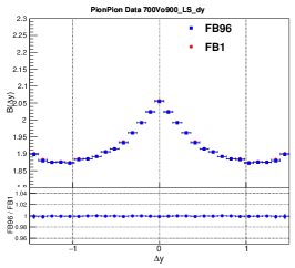
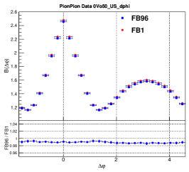
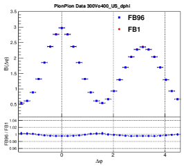
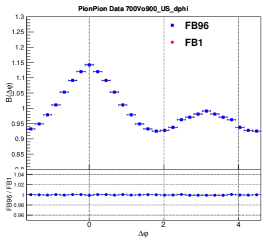
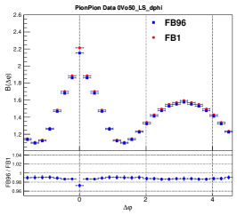
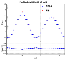
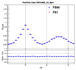
Figure 4.39: For $\pi\pi$ pair. Comparisons of US CF $\Delta y$ (1st row) and $\Delta\varphi$ (3rd row) projections obtained with filter-bit 1 and 96 for 0-5% (left column), 30-40% (middle column), and 70-90% (right column) collision centralities. Comparisons of LS CF $\Delta y$ (2nd row) and $\Delta\varphi$ (4th row) projections obtained with filter-bit 1 and 96 for the same collision centralities.

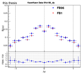
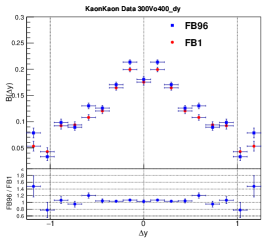
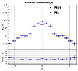
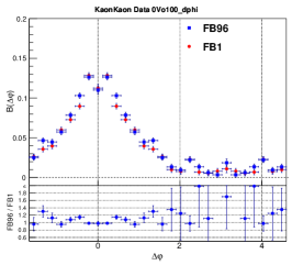
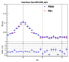
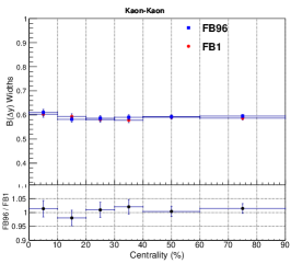
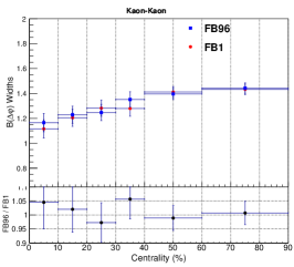
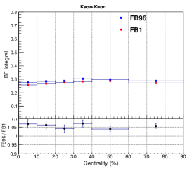
Figure 4.40: Comparisons of $B^{KK}$ projections onto $\Delta y$ (top row) and $\Delta\varphi$ (middle row) axis for selected collision centralities. Bottom row: comparisons of $B^{KK}$ $\Delta y$ widths (left), $\Delta\varphi$ widths (middle), and integrals (right) as a function of collision centrality between filter-bit 1 and 96.

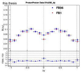
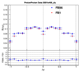
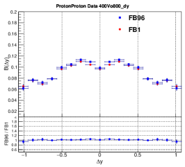
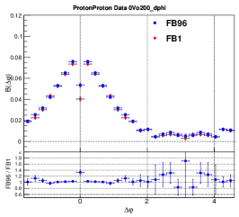
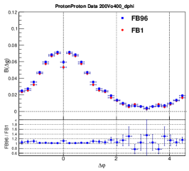
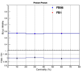
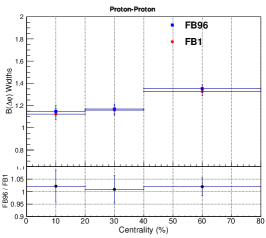
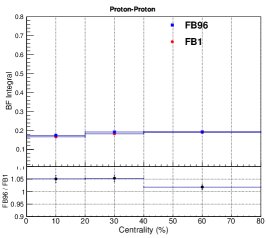
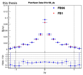
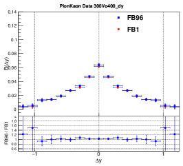
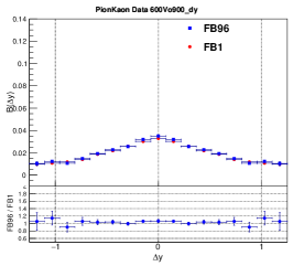
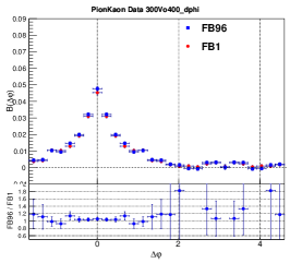
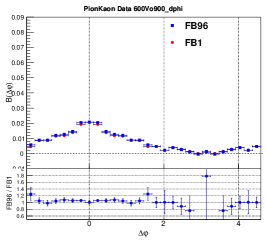
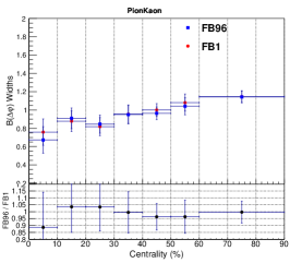
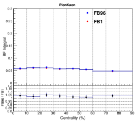
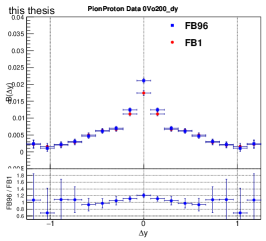
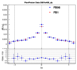
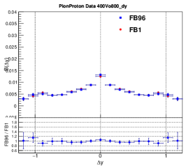
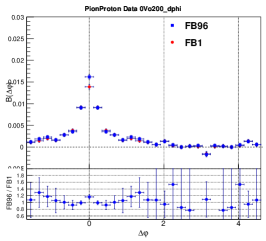
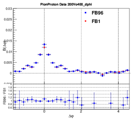
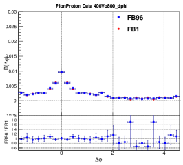
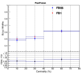
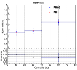
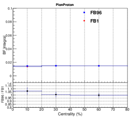
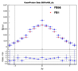
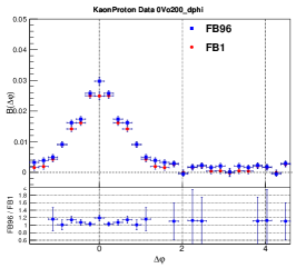
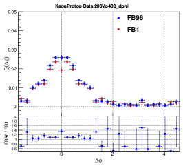
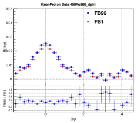
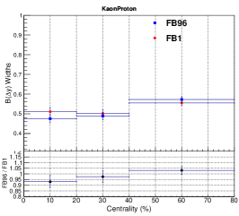
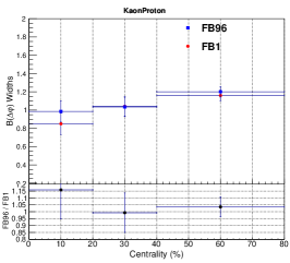
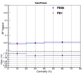
Figure 4.41: Comparisons of $B^{pp}$ projections onto $\Delta y$ (top row) and $\Delta\varphi$ (middle row) axis for selected collision centralities. Bottom row: comparisons of $B^{pp}$ $\Delta y$ widths (left), $\Delta\varphi$ widths (middle), and integrals (right) as a function of collision centrality between filter-bit 1 and 96.

Figure 4.42: Comparisons of $B^{\pi K}$ projections onto $\Delta y$ (top row) and $\Delta\varphi$ (middle row) axis for selected collision centralities. Bottom row: comparisons of $B^{\pi K}$ $\Delta y$ widths (left), $\Delta\varphi$ widths (middle), and integrals (right) as a function of collision centrality between filter-bit 1 and 96.

Figure 4.43: Comparisons of $B^{\pi p}$ projections onto $\Delta y$ (top row) and $\Delta\varphi$ (middle row) axis for selected collision centralities. Bottom row: comparisons of $B^{\pi p}$ $\Delta y$ widths (left), $\Delta\varphi$ widths (middle), and integrals (right) as a function of collision centrality between filter-bit 1 and 96.

Figure 4.44: Comparisons of $B^{Kp}$ projections onto $\Delta y$ (top row) and $\Delta\varphi$ (middle row) axis for selected collision centralities. Bottom row: comparisons of $B^{Kp}$ $\Delta y$ widths (left), $\Delta\varphi$ widths (middle), and integrals (right) as a function of collision centrality between filter-bit 1 and 96.

CHAPTER 5   Systematic Uncertainties

In this work, six possible sources of systematic uncertainties are investigated: magnetic field configurations, $V_{z}$ ranges, PID cuts, additional $p_{\rm T}$-dependent efficiency corrections, track DCA cuts, and TPC number of clusters. The results of these studies are shown in Figures 5.1 – 5.6 for all species pairs considered in this work. Given these studies involve the variation of experimental conditions and cuts, we use the Barlow criterion [43] to determine the magnitude of uncertainties.

The calculation of systematic uncertainties associated with variations of cuts proceeds as follows:

Step 1: For each component, we calculate the bin-by-bin differences ($d$) in BF $\Delta y$ and $\Delta\varphi$ projections along with their widths and integrals between two or more different cuts, as shown in the $2^{nd}$ column of Figs. 5.1 –  5.6 for all species pairs.
Step 2: The difference threshold is set to $D=d/\sqrt{2}$ according to Barlow, in cases where two extreme scenarios are compared.
Step 3: The difference threshold $D$ is subject to the Barlow criterion: if $D>\sqrt{\sigma_{1}^{2}\pm\sigma_{2}^{2}}$ ($+$ for correlated samples; $-$ for uncorrelated samples; $\sigma_{1}$ and $\sigma_{2}$ stand for statistical uncertainties obtained with cut 1 and 2, respectively), then the Barlow criterion $D_{B}$ is set to $D_{B}=D$, otherwise, it is set to $D_{B}=0$, as shown in the $3^{rd}$ column of Figs. 5.1 – 5.6.
Step 4: Systematic uncertainties on $R_{2}^{CD}$ are calculated assuming the six potential sources of uncertainties are statistically independent, by taking a sum in quadrature of the non-vanishing contributions, as shown in Eq.(5).

$$\sigma_{R_{2}^{CD}}=\left[D_{B}^{2}(BField)+D_{B}^{2}(V_{z})+D_{B}^{2}(PID).\right.\\ \left.+D_{B}^{2}(Eff)+D_{B}^{2}(DCA)+D_{B}^{2}(nCluster)\right]^{1/2}.$$

Step 5: Calculate the average of systematic uncertainties of all the bins, denoted ${\bar{\sigma}_{R_{2}^{CD}}}$.
Step 6: For $\Delta y$ and $\Delta\varphi$ projections of balance functions, and their integrals, add, in quadrature, systematic uncertainties of single particle densities of $\pi^{\pm}$, $K^{\pm}$ and $p/\bar{p}$  [8]. Thus, the systematic uncertainties on BF amplitudes are the quadratic sum of systematic uncertainties of CF ($\sigma_{R_{2}^{CD}}$) and the systematic uncertainties from the published single particle densities ($\sigma_{\rho}$), as shown in Eq.(5.1). The values of total systematic uncertainties ($\sigma_{BF}$) are shown in Tables 5.1 – 5.9 for all species pairs.

$$\sigma_{BF}=\sqrt{{{\bar{\sigma}_{R_{2}^{CD}}}}^{2}+\sigma_{\rho}^{2}}$$ (5.1)

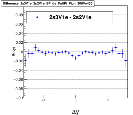
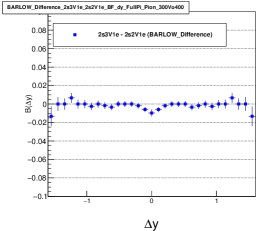
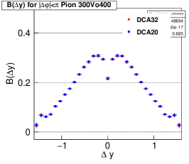
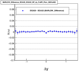
Figure 5.1: Systematic uncertainty contributions in $B^{\pi\pi}(\Delta y)$ from BField ($1^{st}$ row), $V_{z}$ ($2^{nd}$ row), PID ($3^{rd}$ row), and DCA ($4^{th}$ row). The comparisons between two sets of different cuts (left column), with their differences $d$ (middle column), and their differences after the Barlow check $D_{Barlow}$ (right column).

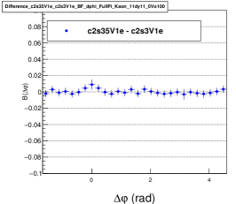
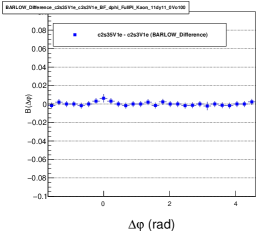
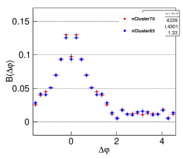
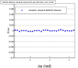
Figure 5.2: Systematic uncertainty contributions in $B^{KK}(\Delta\varphi)$ from BField ($1^{st}$ row), $V_{z}$ ($2^{nd}$ row), PID ($3^{rd}$ row), and nClusters ($4^{th}$ row). The comparisons between two sets of different cuts (left column), with their differences $d$ (middle column), and their differences after the Barlow check $D_{Barlow}$ (right column).

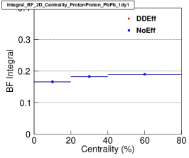
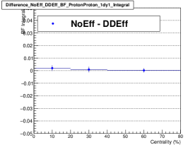
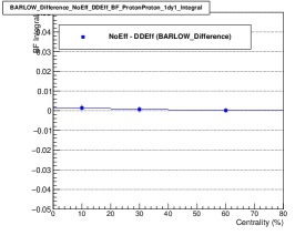
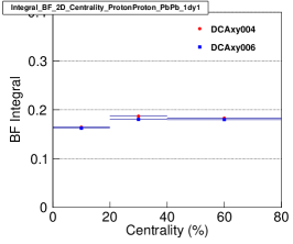
Figure 5.3: Systematic uncertainty contributions in $B^{pp}$ integrals from BField ($1^{st}$ row), PID ($2^{nd}$ row), additional $p_{\rm T}$-dependent efficiency corrections ($3^{rd}$ row), and DCA ($4^{th}$ row). The comparisons between two sets of different cuts (left column), with their differences $d$ (middle column), and their differences after the Barlow check $D_{Barlow}$ (right column).

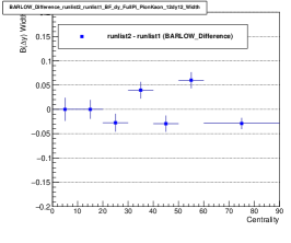
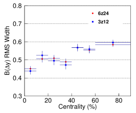
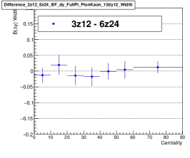
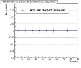
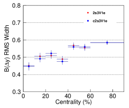
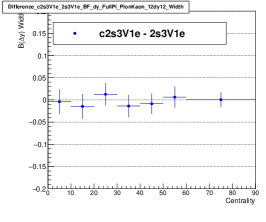
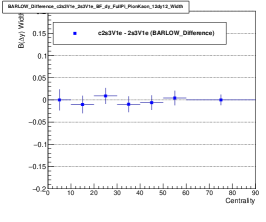
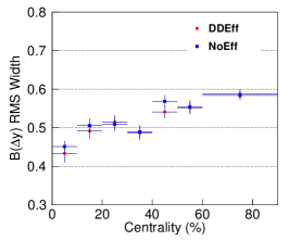
Figure 5.4: Systematic uncertainty contributions in $B^{\pi K}$ $\Delta y$ widths from BField ($1^{st}$ row), $V_{z}$ ($2^{nd}$ row), PID ($3^{rd}$ row), and additional $p_{\rm T}$-dependent efficiency corrections ($4^{th}$ row). The comparisons between two sets of different cuts (left column), with their differences $d$ (middle column), and their differences after the Barlow check $D_{Barlow}$ (right column).

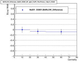
Figure 5.5: Systematic uncertainty contributions in $B^{\pi p}$ $\Delta\varphi$ widths from BField ($1^{st}$ row), $V_{z}$ ($2^{nd}$ row), PID ($3^{rd}$ row), and additional $p_{\rm T}$-dependent efficiency corrections ($4^{th}$ row). The comparisons between two sets of different cuts (left column), with their differences $d$ (middle column), and their differences after the Barlow check $D_{Barlow}$ (right column).

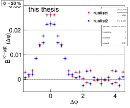
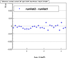
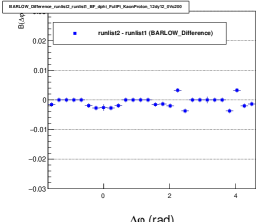
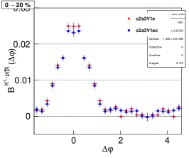
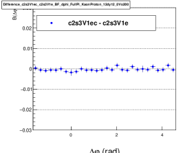
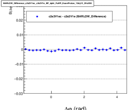
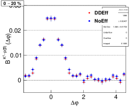
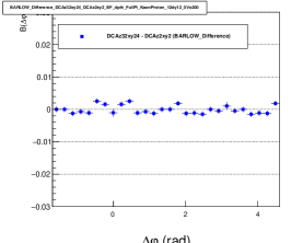
Figure 5.6: Systematic uncertainty contributions in $B^{Kp}(\Delta\varphi)$ from BField ($1^{st}$ row), PID ($2^{nd}$ row), additional $p_{\rm T}$-dependent efficiency corrections ($3^{rd}$ row), and DCA ($4^{th}$ row). The comparisons between two sets of different cuts (left column), with their differences $d$ (middle column), and their differences after the Barlow check $D_{Barlow}$ (right column).

Table 5.1: Total Systematic Uncertainties ($\sigma_{BF}$) on $B^{\pi\pi}$.

Centrality	$B(\Delta y)$	$B(\Delta\varphi)$	$B(\Delta y)$ Width	$B(\Delta\varphi)$ Width	BF Integral
0-5%	0.016	0.011	0.010	0.027	0.030
5-10%	0.015	0.010	0.010	0.027	0.030
10-20%	0.014	0.0097	0.010	0.027	0.030
20-30%	0.014	0.0090	0.010	0.027	0.030
30-40%	0.013	0.0086	0.010	0.027	0.030
40-50%	0.012	0.0088	0.010	0.027	0.030
50-60%	0.010	0.0085	0.010	0.027	0.030
60-70%	0.010	0.0084	0.010	0.027	0.030
70-90%	0.0094	0.0089	0.010	0.027	0.030

Table 5.2: Total Systematic Uncertainties ($\sigma_{BF}$) on $B^{\pi K}$.

Centrality	$B(\Delta y)$	$B(\Delta\varphi)$	$B(\Delta y)$ Width	$B(\Delta\varphi)$ Width	BF Integral
0-10%	0.0041	0.0020	0.033	0.079	0.0072
10-20%	0.0039	0.0022	0.033	0.079	0.0072
20-30%	0.0038	0.0021	0.033	0.079	0.0072
30-40%	0.0035	0.0025	0.033	0.079	0.0072
40-50%	0.0032	0.0023	0.033	0.079	0.0072
50-60%	0.0034	0.0021	0.033	0.079	0.0072
60-90%	0.0031	0.0017	0.033	0.079	0.0072

Table 5.3: Total Systematic Uncertainties ($\sigma_{BF}$) on $B^{\pi p}$.

Centrality	$B(\Delta y)$	$B(\Delta\varphi)$	$B(\Delta y)$ Width	$B(\Delta\varphi)$ Width	BF Integral
0-20%	0.0015	0.00066	0.054	0.053	0.019
20-40%	0.0012	0.00077	0.054	0.053	0.019
40-80%	0.00094	0.00063	0.054	0.053	0.019

Table 5.4: Total Systematic Uncertainties ($\sigma_{BF}$) on $B^{K\pi}$.

Centrality	$B(\Delta y)$	$B(\Delta\varphi)$	$B(\Delta y)$ Width	$B(\Delta\varphi)$ Width	BF Integral
0-10%	0.015	0.0062	0.033	0.079	0.022
10-20%	0.014	0.0060	0.033	0.079	0.022
20-30%	0.012	0.0064	0.033	0.079	0.022
30-40%	0.013	0.0070	0.033	0.079	0.022
40-50%	0.012	0.0059	0.033	0.079	0.022
50-60%	0.012	0.0063	0.033	0.079	0.022
60-90%	0.011	0.0057	0.033	0.079	0.022

Table 5.5: Total Systematic Uncertainties ($\sigma_{BF}$) on $B^{KK}$.

Centrality	$B(\Delta y)$	$B(\Delta\varphi)$	$B(\Delta y)$ Width	$B(\Delta\varphi)$ Width	BF Integral
0-10%	0.024	0.0095	0.016	0.060	0.021
10-20%	0.019	0.0095	0.016	0.060	0.021
20-30%	0.018	0.0094	0.016	0.060	0.021
30-40%	0.018	0.011	0.016	0.060	0.021
40-60%	0.022	0.0090	0.016	0.060	0.021
60-90%	0.015	0.0077	0.016	0.060	0.021

Table 5.6: Total Systematic Uncertainties ($\sigma_{BF}$) on $B^{Kp}$.

Centrality	$B(\Delta y)$	$B(\Delta\varphi)$	$B(\Delta y)$ Width	$B(\Delta\varphi)$ Width	BF Integral
0-20%	0.0046	0.0022	0.068	0.15	0.028
20-40%	0.0037	0.0019	0.068	0.15	0.028
40-80%	0.0047	0.0025	0.068	0.15	0.028

Table 5.7: Total Systematic Uncertainties ($\sigma_{BF}$) on $B^{p\pi}$.

Centrality	$B(\Delta y)$	$B(\Delta\varphi)$	$B(\Delta y)$ Width	$B(\Delta\varphi)$ Width	BF Integral
0-20%	0.012	0.010	0.054	0.053	0.023
20-40%	0.011	0.010	0.054	0.053	0.023
40-80%	0.011	0.010	0.054	0.053	0.023

Table 5.8: Total Systematic Uncertainties ($\sigma_{BF}$) on $B^{pK}$.

Centrality	$B(\Delta y)$	$B(\Delta\varphi)$	$B(\Delta y)$ Width	$B(\Delta\varphi)$ Width	BF Integral
0-20%	0.0092	0.0047	0.068	0.15	0.014
20-40%	0.0075	0.0042	0.068	0.15	0.014
40-80%	0.0090	0.0051	0.068	0.15	0.014

Table 5.9: Total Systematic Uncertainties ($\sigma_{BF}$) on $B^{pp}$.

Centrality	$B(\Delta y)$	$B(\Delta\varphi)$	$B(\Delta y)$ Width	$B(\Delta\varphi)$ Width	BF Integral
0-20%	0.011	0.0051	0.0085	0.067	0.013
20-40%	0.0088	0.0047	0.0085	0.067	0.013
40-80%	0.0098	0.0040	0.0085	0.067	0.013

CHAPTER 6   Results

We have analyzed data from Pb–Pb collisions at $\sqrt{s_{{}_{\rm NN}}}=$2.76 TeV, acquired with the ALICE detector at the Large Hadron Collider, to measure balance functions (BF) of charged hadron pairs $(\pi,K,p)\otimes(\pi,K,p)$. And it is worth to mention that the preliminary results of $B^{\pi\pi}$ and $B^{KK}$ were presented in an oral presentation at the 2018 Quark Matter conference and published in the proceedings [44]. The dataset on which this work is based is presented in Sec. 4.1.1, whereas event and track selection criteria are described in Sec. 4.2. The hadron identification method is introduced in Sec. 4.4, and the detection efficiency correction and optimization methods are reported in Sec. 4.6. Systematic uncertainties are determined according to the methods presented in Chapter 5.

In this Chapter, we present the main results of this dissertation. Two-dimensional balance functions measured as functions of rapidity and azimuth differences are presented in Sec. 6.1, while their projections are discussed in Sec. 6.2. Measurements of the widths and integrals of these balance functions are considered in Sec. 6.3.

6.1   Two-dimensional correlators and balance functions

A complete set of two-dimensional US and LS correlators as well as balance functions, plotted vs. $\Delta y$ and $\Delta\varphi$, for selected collision centralities, is presented in Figs. 6.1 – 6.9 for $\pi\pi$, $\pi K$, $\pi p$, $K\pi$, $KK$, $Kp$, $p\pi$, $pK$ and $pp$ species pairs.

6.1.1   US and LS correlators

US and LS correlators of all the nine species pairs exhibit a collision centrality dependent $\Delta\varphi$ flow-like modulation dominated by the second harmonic cos(2$\Delta\varphi$).

The US correlators of all nine species pairs exhibit similar features but with varying degrees of importance and centrality dependence. Common features include a prominent near-side peak centered at $(\Delta y,\Delta\varphi)=(0,0)$, which varies in width and amplitude with centrality. For example, the $\pi\pi$ US correlator has a broad and strong near-side peak in 70-90% collision centralities, but the peak becomes very narrow in central collisions. Correlators of $\pi K$ and $\pi p$ pairs behave similarly, but their near-side peaks are not as prominent. The correlators of $Kp$ and $pp$ US pairs are rather different. Instead of a near-side peak, they feature a small (shallow and narrow) dip at the origin.

The LS correlators exhibit a mix of interesting features. For example, $\pi\pi$ LS correlators feature a prominent near-side peak which may largely be associated to Hanbury-Brown and Twist (HBT) correlations. The widths of these correlation peaks decrease significantly with system size, whereas the cross-species pairs feature a depression near $(\Delta y,\Delta\varphi)=(0,0)$, which may result in part from Coulomb effects and different source emission velocity and times.

6.1.2   Balance Functions

All nine species pair BFs exhibit common features: a prominent near-side peak centered at $(\Delta y,\Delta\varphi)=(0,0)$ and a relatively flat and featureless away-side. The flat away-side stems for the fact that positive and negative particles of a given species feature essentially equal azimuthal anisotropy relative to the collision symmetry plane. More importantly, it indicates the presence of a fast radial flow profile of the particle emitting sources [6]. For instance, emission from a quasi-thermal source at rest is expected to produce particles nearly isotropically. However, particles produced from such a source traveling at high speed in the lab frame are closely correlated, i.e., emitted at relatively small $\Delta y$ and $\Delta\varphi$.

One notes, however, that the different species pairs feature a mix of near-side peak shapes, widths, magnitudes, and dependences on collision centrality that indicate that they are subject to different charge balancing pair production and transport mechanisms, as well as final state effects. For instance, $B^{\pi\pi}$ exhibits a deep and narrow dip, within the near-side correlation peak, resulting from HBT effects, with a depth and width that vary inversely to the source size (and collision centrality). One observes that $B^{KK}$ exhibits much weaker HBT effects, whereas $B^{pp}$ also features a narrow dip centered at $(\Delta y,\Delta\varphi)=(0,0)$ within a somewhat elongated near-side peak that likely reflects annihilation of $p\bar{p}$ pairs. Produced protons and anti-protons are more likely to annihilate if emitted at small $\Delta y$, $\Delta\varphi$ and $\Delta p_{\rm T}$. Annihilation of $p\bar{p}$ pairs results in the production of several pions (on average), and should thus yield a depletion near the origin $(\Delta y,\Delta\varphi)=(0,0)$ of BFs.

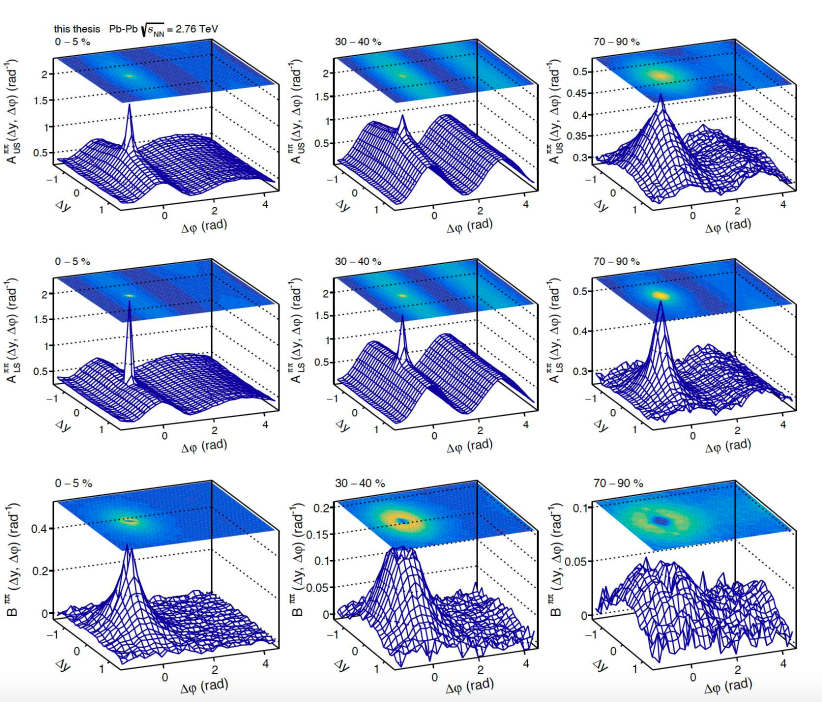
Figure 6.1: Correlation functions and balance functions of $\pi\pi$ pair for selected Pb–Pb collision centralities. Top row: unlike-sign correlation function $A_{US}^{\pi\pi}(\Delta y,\Delta\varphi)$; Middle row: like-sign correlation function $A_{LS}^{\pi\pi}(\Delta y,\Delta\varphi)$; Bottom row: balance function $B^{\pi\pi}(\Delta y,\Delta\varphi)$.

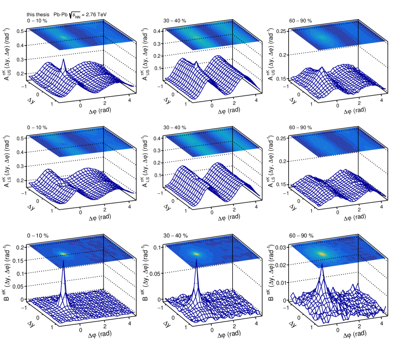
Figure 6.2: Correlation functions and balance functions of $\pi K$ pair for selected Pb–Pb collision centralities. Top row: unlike-sign correlation function $A_{US}^{\pi K}(\Delta y,\Delta\varphi)$; Middle row: like-sign correlation function $A_{LS}^{\pi K}(\Delta y,\Delta\varphi)$; Bottom row: balance function $B^{\pi K}(\Delta y,\Delta\varphi)$.

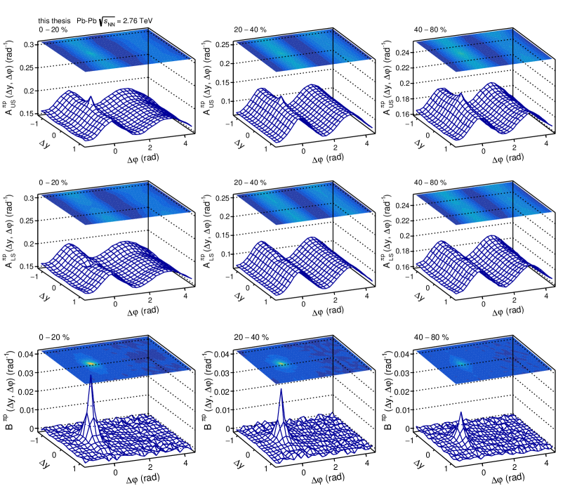
Figure 6.3: Correlation functions and balance functions of $\pi p$ pair for selected Pb–Pb collision centralities. Top row: unlike-sign correlation function $A_{US}^{\pi p}(\Delta y,\Delta\varphi)$; Middle row: like-sign correlation function $A_{LS}^{\pi p}(\Delta y,\Delta\varphi)$; Bottom row: balance function $B^{\pi p}(\Delta y,\Delta\varphi)$.

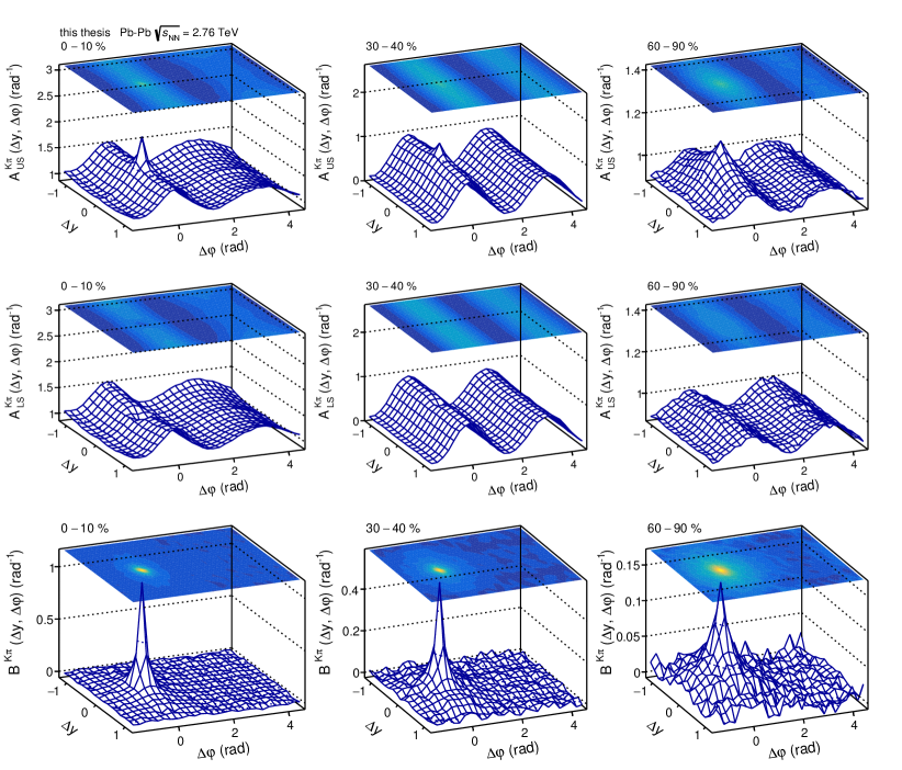
Figure 6.4: Correlation functions and balance functions of $K\pi$ pair for selected Pb–Pb collision centralities. Top row: unlike-sign correlation function $A_{US}^{K\pi}(\Delta y,\Delta\varphi)$; Middle row: like-sign correlation function $A_{LS}^{K\pi}(\Delta y,\Delta\varphi)$; Bottom row: balance function $B^{K\pi}(\Delta y,\Delta\varphi)$.

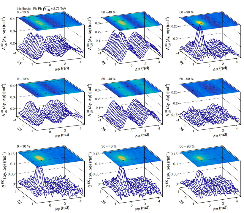
Figure 6.5: Correlation functions and balance functions of $KK$ pair for selected Pb–Pb collision centralities. Top row: unlike-sign correlation function $A_{US}^{KK}(\Delta y,\Delta\varphi)$; Middle row: like-sign correlation function $A_{LS}^{KK}(\Delta y,\Delta\varphi)$; Bottom row: balance function $B^{KK}(\Delta y,\Delta\varphi)$.

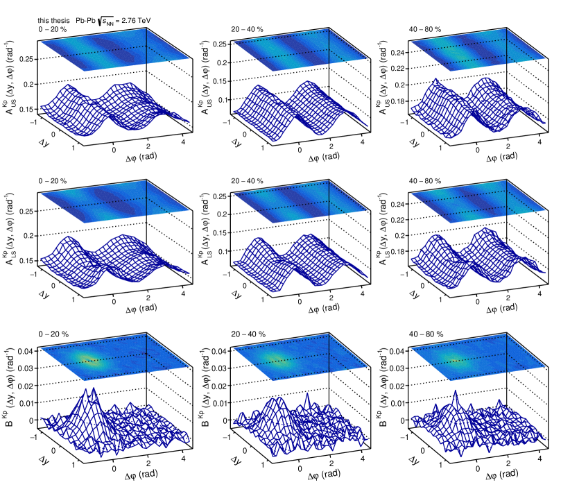
Figure 6.6: Correlation functions and balance functions of $Kp$ pair for selected Pb–Pb collision centralities. Top row: unlike-sign correlation function $A_{US}^{Kp}(\Delta y,\Delta\varphi)$; Middle row: like-sign correlation function $A_{LS}^{Kp}(\Delta y,\Delta\varphi)$; Bottom row: balance function $B^{Kp}(\Delta y,\Delta\varphi)$.

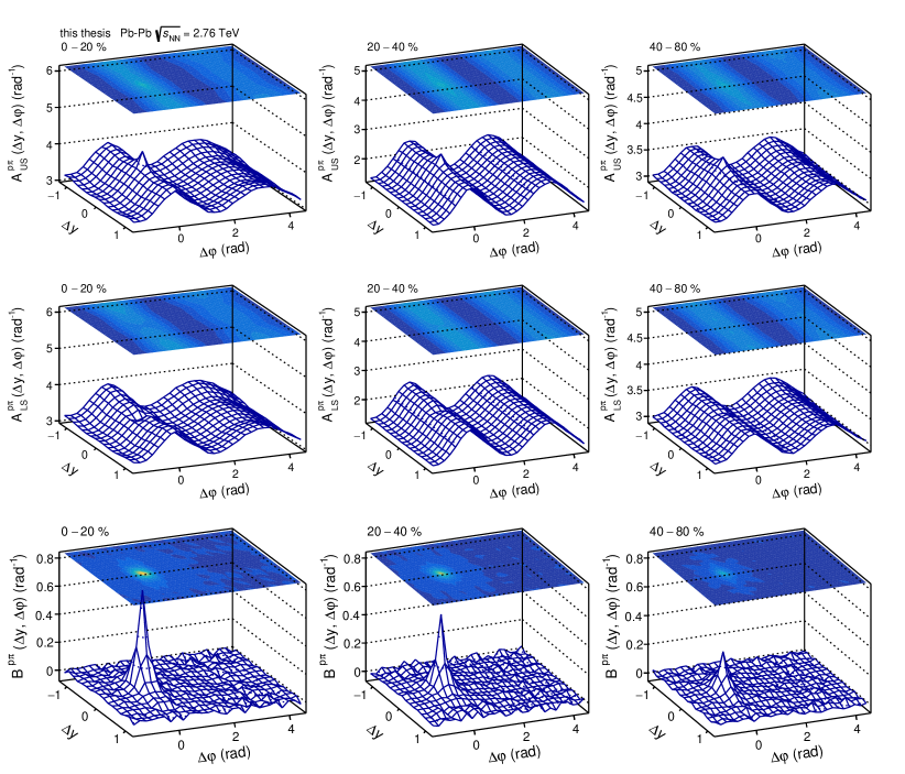
Figure 6.7: Correlation functions and balance functions of $p\pi$ pair for selected Pb–Pb collision centralities. Top row: unlike-sign correlation function $A_{US}^{p\pi}(\Delta y,\Delta\varphi)$; Middle row: like-sign correlation function $A_{LS}^{p\pi}(\Delta y,\Delta\varphi)$; Bottom row: balance function $B^{p\pi}(\Delta y,\Delta\varphi)$.

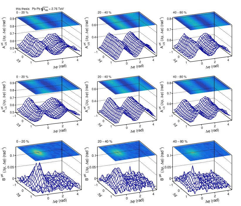
Figure 6.8: Correlation functions and balance functions of $pK$ pair for selected Pb–Pb collision centralities. Top row: unlike-sign correlation function $A_{LS}^{pK}(\Delta y,\Delta\varphi)$; Middle row: like-sign correlation function $A_{LS}^{pK}(\Delta y,\Delta\varphi)$; Bottom row: balance function $B^{pK}(\Delta y,\Delta\varphi)$.

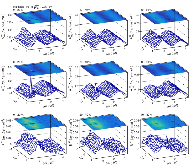
Figure 6.9: Correlation functions and balance functions of $pp$ pair for selected Pb–Pb collision centralities. Top row: unlike-sign correlation function $A_{US}^{pp}(\Delta y,\Delta\varphi)$; Middle row: like-sign correlation function $A_{LS}^{pp}(\Delta y,\Delta\varphi)$; Bottom row: balance function $B^{pp}(\Delta y,\Delta\varphi)$.

6.2   Balance Function Projections

We further examine the collision centrality evolution of the nine species pair BFs by plotting their projections onto the $\Delta y$ axis in Fig. 6.10. We find that the $\Delta y$ projection shape and amplitude of $B^{\pi\pi}$ exhibit the strongest centrality dependence, whereas those of $B^{\pi K}$, $B^{\pi p}$, $B^{K\pi}$, $B^{p\pi}$, and $B^{pp}$ display significant albeit smaller dependence on centrality. The $\Delta y$ projections of $B^{KK}$, $B^{Kp}$, and $B^{pK}$, on the other hand, feature minimal centrality dependence, if any.

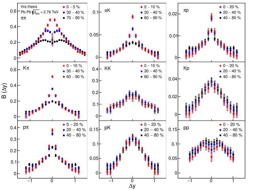
Figure 6.10: Longitudinal ($\Delta y$) projections of balance functions for $|\Delta\varphi|\leq\pi$ of the full species matrix of $\pi^{\pm}$, $K^{\pm}$ and $p/\bar{p}$, with $\pi^{\pm}$, $K^{\pm}$ and $p/\bar{p}$ as reference particle in the $1^{st}$, $2^{nd}$ and $3^{rd}$ row, respectively. Systematic uncertainties are shown as boxes.

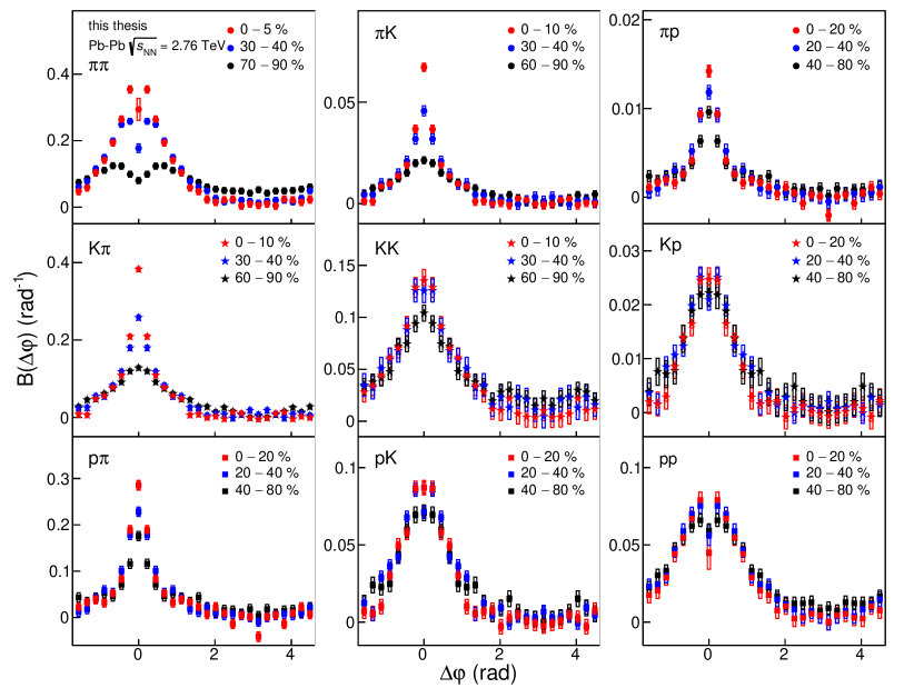
Figure 6.11: BF $\Delta\varphi$ projections of the full species matrix of $\pi^{\pm}$, $K^{\pm}$ and $p/\bar{p}$, with $\pi^{\pm}$, $K^{\pm}$ and $p/\bar{p}$ as the interest particle in the $1^{st}$, $2^{nd}$ and $3^{rd}$ row, respectively. Systematic uncertainties are shown as boxes.

The BF $\Delta\varphi$ projections of the full species matrix of $\pi^{\pm}$, $K^{\pm}$ and $p/\bar{p}$ are presented in Figure 6.11. We find that the $\Delta\varphi$ projection shape and amplitude of $B^{\pi\pi}$ exhibit the strongest centrality dependence, whereas those of $B^{\pi K}$, $B^{\pi p}$, $B^{K\pi}$ and $B^{p\pi}$, display significant albeit smaller dependence on centrality. The $\Delta\varphi$ projections of $B^{KK}$, $B^{Kp}$, $B^{pK}$, and $B^{pp}$ on the other hand, feature minimal centrality dependence, if any.

6.3   BF RMS Widths and Integrals

We characterize the collision centrality evolution of the shape and strength of the BFs in terms of their longitudinal and azimuthal rms widths, as well as their integrals in Fig. 6.12. One thing to note is that, the points of the $\Delta y$ and $\Delta\varphi$ projections are not included in the rms calculations, if they are smaller than 0. However, all the points of the $\Delta y$ and $\Delta\varphi$ projections are included in the BF integral calculations.

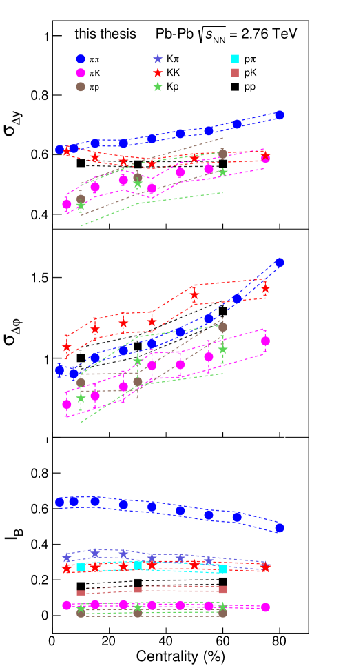
Figure 6.12: $\Delta y$ rms widths (top), $\Delta\varphi$ rms widths (middle), and integrals (bottom) of BFs of the full species matrix of $\pi^{\pm}$, $K^{\pm}$ and $p/\bar{p}$ as a function of collision centrality. For $\Delta y$ and $\Delta\varphi$ widths, $K\pi$, $p\pi$ and $pK$ have the same values with $\pi K$, $\pi p$, and $Kp$, respectively. The relative azimuthal angle range for all the species pairs is $|\Delta\varphi|\leq\pi$. The relative rapidity range for all the species pairs is $|\Delta y|\leq 1.2$, with exceptions that for $\pi\pi$ it is $|\Delta y|\leq 1.4$, while for $pp$ it is $|\Delta y|\leq 1.0$. Systematic uncertainties are shown as dashed lines.

The BFs of all measured species combinations exhibit a strong narrowing in azimuth from peripheral to central collisions (e.g., 50% for $\pi\pi$ pair). Such narrowing, already observed for unidentified charged hadrons at both RHIC and LHC energies, and for pions at RHIC, is commonly ascribed to strong radial collective motion with average velocities that monotonically increase towards central collisions [6]. In the longitudinal direction, the BF of all species pairs, except those of $KK$ and $pp$, also exhibit significant narrowing from peripheral to central collision. We find that the longitudinal projections and rms of $KK$ pairs display no dependence on collision centrality. However, we remark that while the longitudinal rms of $B^{pp}$ are essentially invariant, their projections do change shape with collision centrality. This apparent contradiction results largely from the limited longitudinal acceptance of the $pp$ BF measurements. It is also worth noticing that longitudinal rms values of cross-species pairs are rather similar and considerably smaller than those of $\pi\pi$ pair. By contrast, the azimuthal rms of all pairs exhibit a wide spread of values, with $KK$ pairs featuring the largest values while $\pi K$ pairs feature the smallest. Qualitatively, one expects that radial flow boosts should have a larger impact on heavier pair progenitors (the objects that decay or produce the observed correlated pairs), thereby yielding narrowest azimuthal BFs for those pairs. However, $\pi\pi$ and $pp$ feature similar rms widths in azimuth but rather different longitudinal widths therefore suggesting that other mechanisms are at play in determining the shape and widths of their respective balance functions. The B($\Delta y$) width results indicate that the balancing pair production mechanisms of $K^{\pm}$ and $p/\bar{p}$ are rather different from those of $\pi^{\pm}$. On the one hand, the $KK$ results are qualitatively consistent with the two-wave quark production scenario, which stipulates that the production of up and down quarks dominates the late stage whereas strange quarks are predominantly produced during the early stages of collisions. On the other hand, the broad $pp$ BFs, whose widths are not fully captured in Fig. 6.12, suggest that baryon anti-baryon pair creation might also occur rather early in A–A collisions.

Shifting our attention to the bottom panel of Figure 6.12, which displays the collision centrality evolution of integrals, noted $I_{B}^{\alpha\beta}$, of BFs of all nine species pairs $\alpha\beta$, we note that $I_{B}^{\pi\pi}$ exhibits a modest increasing trend towards central collisions whereas integrals of other species pairs are essentially invariant. By construction, integrals of $B^{\alpha\beta}(\Delta y,\Delta\varphi)$, reported for the first time in this work, measure the probability of observing a charge balancing (i.e., an associated) particle of species $\beta$ given a reference particle of species $\alpha$ has been observed. We may thus call $I_{B}^{\alpha\beta}$ hadron species pairing probability. Results shown in Fig. 6.12 are surprising on two accounts. First, the lack of collision centrality dependence of integrals $I_{B}^{\alpha\beta}$ observed for all species pairs, but one, imply hadron species pairing probabilities are invariant with collision centrality. Second, close examination of these hadron species pairing probabilities show they are rather different than inclusive probabilities of observing $\pi^{\pm}$, $K^{\pm}$, and $p/\bar{p}$ in Pb–Pb collisions. For instance, $I_{B}^{K\pi}$ is not larger than $I_{B}^{KK}$ by the $\pi/K$ ratio of inclusive single particle yields [8] and $I_{B}^{pp}$ is larger than $I_{B}^{pK}$ also in contrast to observed ratios of $K/p$ yield ratios. Hadron pairing probabilities are thus indeed very different than the relative probabilities of single hadrons. Note that the observed rise of $I_{B}^{\pi\pi}$ in more central collisions may artificially result from increased kinematic focusing of pions with centrality in the $p_{\rm T}$ and $\Delta y$ acceptance of this measurement. The higher velocity flow fields encountered in more central Pb–Pb collisions could indeed shift and focus the yield of associated pions. Why such a shift is not as important for other charge balancing pairs remains to be elucidated with a comprehensive model accounting for the flow velocity profile and appropriate sets of charge conserving processes yielding balancing charges in the final state of collisions. Recent deployment of hydrodynamics models feature the former but lack the latter. Further theoretical work is thus required to interpret the observed collision centrality dependence of the hadron species pairing probabilities displayed in Fig. 6.12.

CHAPTER 7   Summary

In summary, we presented first measurements of the collision centrality evolution of balance functions (BF) of the full species matrix of charged hadrons, $(\pi,K,p)\otimes(\pi,K,p)$ in Pb-Pb collisions at $\sqrt{s_{{}_{\rm NN}}}=$2.76 TeV. Measured as functions of particle pair separation in rapidity ($\Delta y$) and azimuth ($\Delta\varphi$), the BFs exhibit a common prominent near-side peak centered at $(\Delta y,\Delta\varphi)=(0,0)$. The peaks with different species pairs feature different shapes, amplitudes, and widths, and varied dependences on collision centrality. The BFs of all species pairs feature narrowing $\Delta\varphi$ rms widths in more central collisions, owing to the strong radial flow field present in central Pb–Pb collisions. In the longitudinal direction, the rms widths of BFs of all species pairs narrow with centrality except for those of $KK$ and $pp$ pairs. The shape and width of $KK$ BFs are invariant with collision centrality, while the $pp$ BFs exhibit some shape dependence on collision centrality but essentially invariant rms values with the acceptance of the measurement. The observed centrality invariance of the $KK$ longitudinal and narrowing rms of other species in the longitudinal direction are qualitatively consistent with effects associated with radial flow and the two-wave quark production scenario. However, a comprehensive model accounting for hadron chemistry at finite temperature, charge conserving pair creation, and strong radial flow fields is required in order to interpret the data presented in greater detail.

Advisor:	Prof. Claude Pruneau
Major:	Physics
Degree:	Doctor of Philosophy

We present the first balance function (BF) measurement of charged hadron pairs $(\pi,K,p)\otimes(\pi,K,p)$ in Pb–Pb collisions at $\sqrt{s_{{}_{\rm NN}}}=$2.76 TeV. The BF measurements are carried out as two-dimensional (2D) differential correlators vs. the relative rapidity ($\Delta y$) and azimuthal angle ($\Delta\varphi$) of hadron pairs, and studied as a function of collision centrality. While the BF azimuthal widths of all pairs substantially decrease from peripheral to central collisions, the longitudinal widths exhibit mixed behaviors: BF of $\pi\pi$ and cross-species pairs narrow in more central collisions whereas those of $KK$ and $pp$ are found invariant with collision centrality. This dichotomy is qualitatively consistent with the presence of strong radial flow effects and the existence of two waves of quark production in relativistic heavy ion collisions. We additionally present first measurements of the BF integrals and find that hadron pairing probabilities are very different from single hadron ratios and feature minimal collision centrality dependence. Overall, the results presented provide new and challenging constraints for theoretical models of hadron production and transport in relativistic heavy ion collisions.

Bibliography

- [1] Scott Pratt. Identifying the charge carriers of the quark-gluon plasma. Phys. Rev. Lett., 108:212301, May 2012.
- [2] ALICE Collaboration. Flow dominance and factorization of transverse momentum correlations in pb-pb collisions at the lhc. Phys. Rev. Lett., 118:162302, Apr 2017.
- [3] ALICE Collaboration. Two particle differential transverse momentum and number density correlations in p-Pb and Pb-Pb at the LHC. 2018.
- [4] Shantam Ravan, Prabhat Pujahari, Sidharth Prasad, and Claude A. Pruneau. Correcting correlation function measurements. Phys. Rev. C, 89:024906, Feb 2014.
- [5] Steffen A. Bass, Pawel Danielewicz, and Scott Pratt. Clocking hadronization in relativistic heavy-ion collisions with balance functions. Phys. Rev. Lett., 85:2689–2692, Sep 2000.
- [6] Sergei A. Voloshin. Transverse radial expansion in nuclear collisions and two particle correlations. Physics Letters B, 632(4):490 – 494, 2006.
- [7] Y. J. Ye, Y. G. Ma, A. H. Tang, and G. Wang. Effect of magnetic fields on pairs of oppositely charged particles in ultrarelativistic heavy-ion collisions. Phys. Rev. C, 99:044901, Apr 2019.
- [8] ALICE Collaboration. Centrality dependence of , , and production in pb-pb collisions at tev. Phys. Rev. C, 88:044910, Oct 2013.
- [9] S. Pratt. Balance functions: A signal of late-stage hadronization. Nuclear Physics A, 698(1):531 – 534, 2002. 15th Int. Conf. on Ultra-Relativistic Nucleus-Nucleus Collisions (Quark Matter 2001).
- [10] STAR Collaboration. Narrowing of the balance function with centrality in collisions at . Phys. Rev. Lett., 90:172301, May 2003.
- [11] STAR Collaboration. Net charge fluctuations in collisions at . Phys. Rev. C, 68:044905, Oct 2003.
- [12] Piotr Bozek. The balance function in azimuthal angle is a measure of the transverse flow. Physics Letters B, 609(3):247 – 251, 2005.
- [13] Piotr Bozek and Wojciech Broniowski. Charge balancing and the fall off of the ridge. Nuclear Physics A, 904-905:479c – 482c, 2013. The Quark Matter 2012.
- [14] Scott Pratt. General charge balance functions: A tool for studying the chemical evolution of the quark-gluon plasma. Phys. Rev. C, 85:014904, Jan 2012.
- [15] STAR Collaboration. Balance functions from , , and collisions at gev. Phys. Rev. C, 82:024905, Aug 2010.
- [16] Scott Pratt. Viewing the Chemical Evolution of the Quark-Gluon Plasma with Charge Balance Functions. PoS, CPOD2013:023, 2013.
- [17] Sangyong Jeon and Scott Pratt. Balance functions, correlations, charge fluctuations, and interferometry. Phys. Rev. C, 65:044902, Apr 2002.
- [18] A Bialas. Balance functions in coalescence model. Physics Letters B, 579(1):31 – 38, 2004.
- [19] A. Bialas and J. Rafelski. Balance of baryon number in the quark coalescence model. Physics Letters B, 633(4):488 – 491, 2006.
- [20] W. Florkowski, W. Broniowski, and P. Bozek. Production of resonances in a thermal model: Invariant mass spectra and balance functions. J. Phys., G30:S1321–S1324, 2004.
- [21] Scott Pratt and Sen Cheng. Removing distortions from charge balance functions. Phys. Rev. C, 68:014907, Jul 2003.
- [22] Bo Ling, Todd Springer, and Mikhail Stephanov. Hydrodynamics of charge fluctuations and balance functions. Phys. Rev. C, 89:064901, Jun 2014.
- [23] Sen Cheng, Silvio Petriconi, Scott Pratt, Michael Skoby, Charles Gale, Sangyong Jeon, Vasile Topor Pop, and Qing-Hui Zhang. Statistical and dynamic models of charge balance functions. Phys. Rev. C, 69:054906, May 2004.
- [24] Jun Song, Feng-lan Shao, and Zuo-tang Liang. Quark charge balance function and hadronization effects in relativistic heavy ion collisions. Phys. Rev. C, 86:064903, Dec 2012.
- [25] Na Li, Zhiming Li, and Yuanfang Wu. Longitudinal boost invariance of the charge balance function in hadron-hadron and nucleus-nucleus collisions. Phys. Rev. C, 80:064910, Dec 2009.
- [26] STAR Collaboration. Longitudinal scaling property of the charge balance function in au+au collisions at snn=200 gev. Physics Letters B, 690(3):239 – 244, 2010.
- [27] STAR Collaboration. Beam-energy dependence of charge balance functions from au + au collisions at energies available at the bnl relativistic heavy ion collider. Phys. Rev. C, 94:024909, Aug 2016.
- [28] ALICE Collaboration. Charge correlations using the balance function in pb– pb collisions at tev. Physics Letters B, 723(4):267 – 279, 2013.
- [29] ALICE Collaboration. Multiplicity and transverse momentum evolution of charge-dependent correlations in pp, p–Pb, and Pb–Pb collisions at the LHC. Eur. Phys. J., C76(2):86, 2016.
- [30] Jinjin Pan. Multiplicity and transverse momentum evolution of charge-dependent correlations in pp, p-Pb, and Pb-Pb collisions at the LHC. J. Phys. Conf. Ser., 832(1):012044, 2017.
- [31] Scott Pratt, William Patrick McCormack, and Claudia Ratti. Production of charge in heavy ion collisions. Phys. Rev. C, 92:064905, Dec 2015.
- [32] ALICE Collaboration. The ALICE experiment at the CERN LHC. JINST, 3:S08002, 2008.
- [33] ALICE Collaboration. ALICE: Physics performance report, volume II. J. Phys., G32:1295–2040, 2006.
- [34] ALICE Collaboration. ALICE technical design report of the inner tracking system (ITS). CERN-LHCC-99-12, 1999.
- [35] J. Alme et al. The alice tpc, a large 3-dimensional tracking device with fast readout for ultra-high multiplicity events. Nuclear Instruments and Methods in Physics Research Section A: Accelerators, Spectrometers, Detectors and Associated Equipment, 622(1):316 – 367, 2010.
- [36] A. Akindinov et al. Performance of the ALICE Time-Of-Flight detector at the LHC. Eur. Phys. J. Plus, 128:44, 2013.
- [37] ALICE Collaboration. Performance of the ALICE Experiment at the CERN LHC. Int. J. Mod. Phys., A29:1430044, 2014.
- [38] Miklos Gyulassy and Xin-Nian Wang. HIJING 1.0: A Monte Carlo program for parton and particle production in high-energy hadronic and nuclear collisions. Comput. Phys. Commun., 83:307, 1994.
- [39] ALICE Collaboration. Centrality determination of Pb-Pb collisions at = 2.76 TeV with ALICE. Phys. Rev., C88(4):044909, 2013.
- [40] Shantam Ravan, Prabhat Pujahari, Sidharth Prasad, and Claude A. Pruneau. Correcting Correlation Function Measurements. Phys. Rev., C89(2):024906, 2014.
- [41] Victor Gonzalez, Ana Marin, Pedro Ladron de Guevara, Jinjin Pan, Sumit Basu, and Claude A. Pruneau. Effect of centrality bin width corrections on two-particle number and transverse momentum differential correlation functions. Phys. Rev. C, 99:034907, Mar 2019.
- [42] ALICE Collaboration. Insight into particle production mechanisms via angular correlations of identified particles in pp collisions at TeV. Eur. Phys. J., C77(8):569, 2017.
- [43] Roger Barlow. Systematic errors: Facts and fictions. In Advanced Statistical Techniques in Particle Physics. Proceedings, Conference, Durham, UK, March 18-22, 2002, pages 134–144, 2002.
- [44] Jinjin Pan. Balance functions of (un)identified hadrons in pb–pb, p–pb, and pp collisions at the lhc. Nuclear Physics A, 982:315 – 318, 2019. The 27th International Conference on Ultrarelativistic Nucleus-Nucleus Collisions: Quark Matter 2018.
ABSTRACT