Mathematics underfoot:
The formulas that came to Würzburg from New Haven

Two formulas are set in floor-tiles in the foyer of the Würzburg building that houses the laboratory in which Wilhelm Röntgen discovered X-rays in 1895. But what do they mean, and what have they got to do with Röntgen or his work? The answers involve two distinguished professors and their PhD students, working on opposite sides of the Atlantic in the $19$th Century.

1 Playing detective

On a trip to the German city of Würzburg in 2016 I visited the memorial honouring Wilhelm Röntgen, who discovered X-rays there in 1895 and who was awarded the first Nobel Prize in Physics in 1901 as a result.

At the time of his discovery Röntgen was Professor and Head of the Institute of Physics at Julius-Maximilians-Universität (JMU) Würzburg. His laboratory is preserved, complete with much of his equipment, in a building that is open to the public and that is now part of the University of Applied Sciences Würzburg-Schweinfurt.

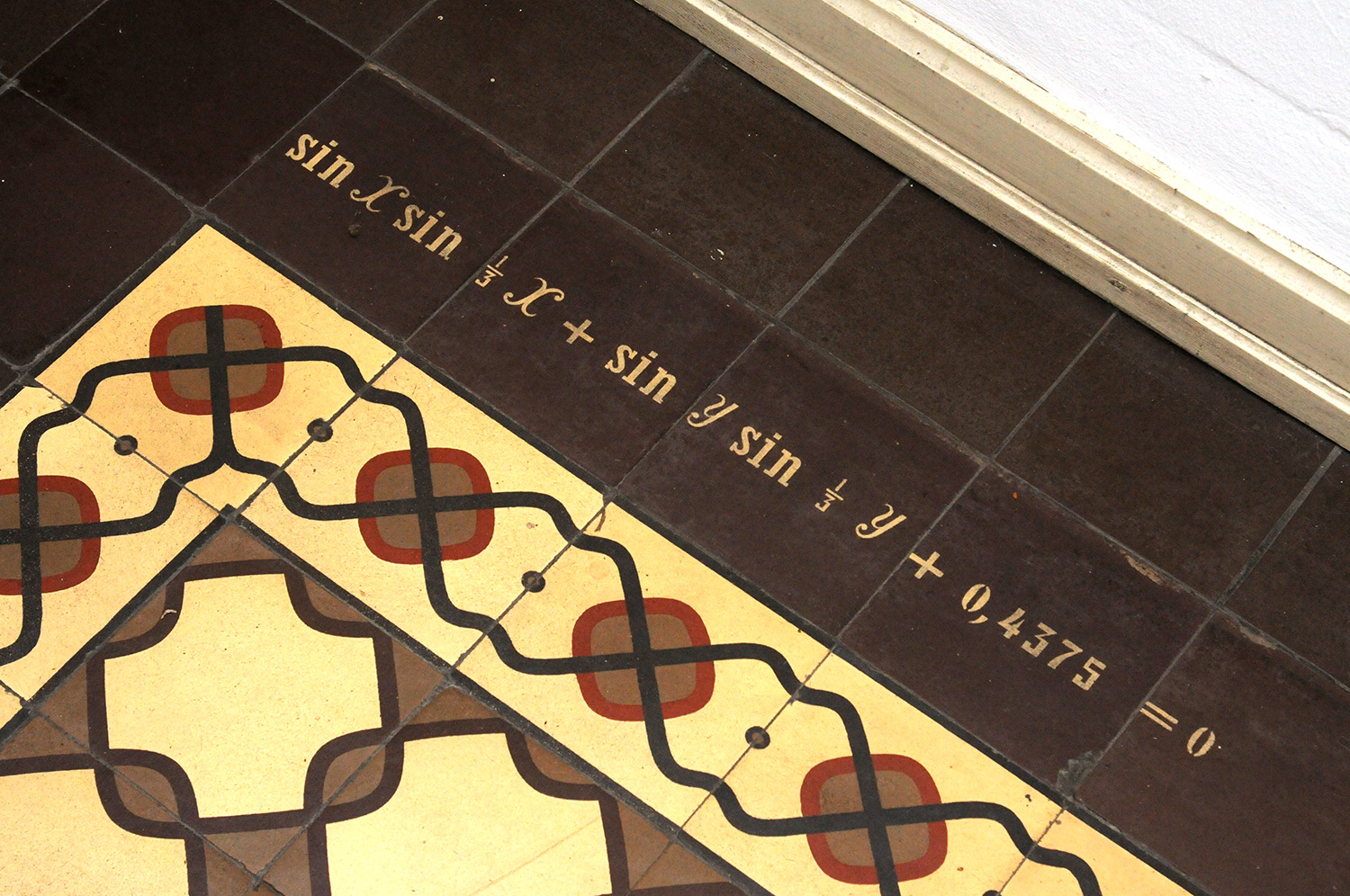
Figure 1: Part of the foyer floor, showing the first formula. Photo courtesy of G. Bartsch.

In the foyer, two trigonometrical formulas are set in the tiled floor. No explanation is provided for these formulas, and no hint given as to their connection with Röntgen’s work. The two formulas are

$$\quad\sin(x)\,\sin(x/3)+\sin(y)\,\sin(y/3)+0.4375=0\,,$$ (1)

$$\quad\sin(y)\,\sin(y/2)=1.3685\,\sin(x)\,\sin(x/3)\,.$$

Following my visit, I contacted several colleagues in the international physics and mathematics communities, but none could throw any light on the meaning of the formulas.

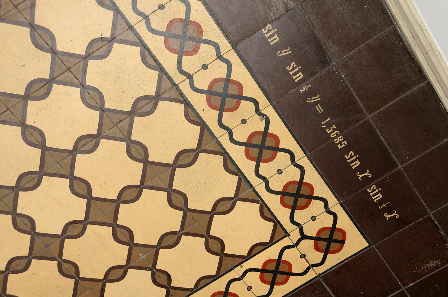
Figure 2: Part of the foyer floor, showing the second formula. Photo courtesy of G. Bartsch.

It occurred to me and a Queensland colleague Dr. Vincent Hart, to treat the formulas as coupled equations in two unknowns, but this led to pairs of numbers of no apparent importance. Frustrated by my continuing ignorance, I contacted Mr. Gunnar Bartsch in the Press and Public Relations Section of JMU Würzburg, but he could not tell me more, though he did supply me with clear pictures of the formulas in the foyer, as in Figs. 1 and 2.

I must add that when Dr. Peter Jarvis of the University of Tasmania saw these pictures, he suggested that the formulas might be connected to the pattern of tiles on the floor next to them, also shown in Figs. 1 and 2. In view of what was revealed later, I am somewhat ashamed to admit that had not occurred to me; I had it fixed in my mind that the formulas must have something to do with Röntgen and his work.

The first breakthrough came when I had a letter published [2] seeking further information from the international physics community about the formulas. This aroused the interest of Emer. Prof. Steve Webb of the Royal Cancer Hospital, London. He asked a German colleague, Prof. Wolfgang Schlegel of the German Cancer Research Centre in Heidelberg if he could throw any light on the mystery, and Schlegel in turn passed the question to Prof. Robert Grebner, President of the University of Applied Sciences Würzburg-Schweinfurt, the present owners of the building. As a result Schlegel [3] and in turn Webb and I, were provided with a copy of an article written by journalist Ernst Nöth about the formulas, published in the local Würzburg newspaper Main–Post back in 1971 [4].

From this article we learned that the tiled floor was designed around 1876, at the time the building that would eventually house Röntgen’s laboratory was being planned by Friedrich Kohlrausch, who was Röntgen’s predecessor as Professor in the Institute of Physics at JMU Würzburg. The tiling was completed together with the rest of the building by 1879, and so has nothing at all to do with Röntgen or X-rays. The two formulas refer to, and in fact define, the patterns on the tiles next to them on the floor, as the article makes clear with an accompanying computer-generated picture of the curves defined by the first formula.

The article quotes from a hand-written account by Kohlrausch of the planning of the building and its construction, in which he says that his Research Assistant Vincenc Strouhal got the idea for the floor pattern from “an American paper by Newton and Philipps (sic)”, and that the tiles were produced by the firm of “Villeroy and Koch (sic)” under the supervision of an engineer named Hrn. Ubach.

Now I knew the meaning of the formulas and something of their history, but was this as much as could be uncovered about them? After generating pictures from the two formulas (1) using MATLAB [5], shown here in Figs. 3 and 4 and closely matching the inner and outer patterns seen on the tiles in Fig. 1 and 2, I was able to show that the numbers $0.4375$ and $1.3685$ appearing there are approximations to exact critical values $7/16$ and $64\sqrt{3}/81$ at which each of the two sets of curves becomes most closely connected, as discussed in Appendices A and B below. But despite searching on the Internet, I could not locate any paper by “Newton and Philipps (or Phillips or Philips)”.

Then came the second major breakthrough. Gunnar Bartsch published an article describing the story to this point [6], reproduced in Main-Post [7], including a note that Anja Schlömerkemper, Professor of Mathematics at JMU Würzburg, had also confirmed using the computer that the formulas (1) do indeed define the inner and outer parts of the pattern on the tiles. More important for what followed, Bartsch included the remark by Kohlrausch about an “American paper by Newton and Philipps”. Dr. Matthias Reichling of the Computing Center of JMU Würzburg am Hubland saw the article and, more skilful at searching the Internet than I, located the paper online [8] and provided me with details.

From this point I was able to discover much of the background about Newton and Kohlrausch and their respective PhD students, Phillips and Strouhal, and to fill in the story of the tiled floor in Würzburg as told below, using some judicious guesswork as to how the numbers in the formulas (1) were chosen, and how Strouhal must have designed the tiles, re-working hand-drawn figures in the paper by Newton and Phillips [8].

Join me now in a trip back in time $\dots$.

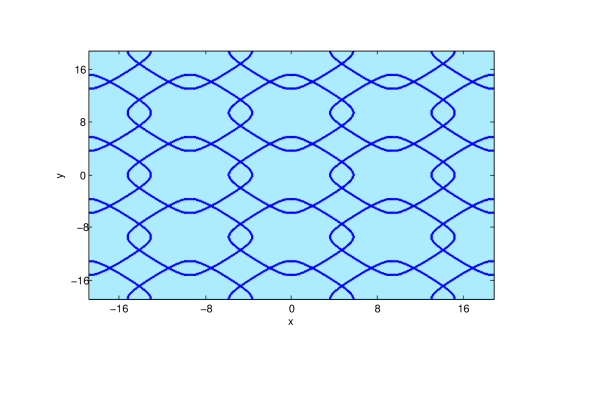
Figure 3: Computer-generated curves defined by the first of formulas (1), over four periods in $x$ and $y$, from $-6\pi$ to $6\pi$.

2 How it may have happened

It is 1875 in New Haven, Connecticut, where Hubert Anson Newton at age 45 has already been Professor and Head of Mathematics at Yale University for 20 years, during which he has supervised a number of successful PhD students, including J. Willard Gibbs, who is now Professor of Mathematical Physics at Yale. Newton himself has done important work in pure mathematics and actuarial methods, but he also manages the Observatory at Yale, and has established an international reputation for his work on the paths of meteors and comets [9, 10]. He is a Charter Member of the National Academy of Sciences of the United States and is a Vice-President, later to be President, of the American Association for the Advancement of Science (AAAS). In 1892 he will be elected a Foreign Member of the Royal Society of London.

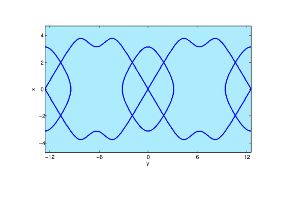
Figure 4: Computer-generated curves defined by the second of formulas (1), over one period in $x$, from $-3\pi/2$ to $3\pi/2$, and two periods in $y$, from $-4\pi$ to $4\pi$.

By 1875 Newton has taken under his wing 31 year old Andrew Wheeler Phillips, a gifted student with an unusual mathematical background. Until accepted into Newton’s Graduate School class without the usual prerequisite of a Bachelor’s degree, he has been largely self-taught [11]. Phillips will complete his PhD thesis “On three-bar motion” in 1877, building on recent work by Roberts [12] and Cayley [13], and will later go on himself to become Professor of Mathematics and Dean of the Graduate School at Yale. During his career, he will co-author a variety of influential mathematical texts, notably one on the graphical interpretation of equations [14].

Motivated perhaps by Newton’s work on comets, or by Phillips’ thesis topic, the two co-author a paper in 1875 in the Transactions of the Connecticut Academy of Arts and Sciences (CAAS) on the curves in the Cartesian plane defined by certain transcendental equations [8]. After noting that “attempts to classify the numerous varieties of transcendental curves have been rare”, and that it is not easy from the form of such a curve “to state an equation that can represent it”, they remark that “the simpler inverse problem of describing the curve from the equation is naturally the first to be undertaken” in the hope that “the forms that result may, when compared, suggest the solution of the direct problem”.

For their study, they choose equations of the form

$$\sin(y)\,\sin(my)=a\sin(x)\,\sin(nx)+b\,,$$ (2)

where $m<1$ and $n<1$ are positive constants, mostly taken to be rational with denominators no greater than $11$, while $a$ and $b$ are more general real constants.

In a series of 24 plates, they present the curves for over 100 different cases, each one obtained by first calculating the coordinates of a sufficiently large number of points to determine a corresponding hand-drawn graph accurately. This in turn requires the determination of all solutions of a large number of equations of the form

$$\sin(x)\,\sin(mx)=c\,$$ (3)

“by trial and error, a very simple process, but when often repeated quite tedious” [8]. They note that as the values of the constants in (2) are varied, the curves can close or open to form a multitude of patterns, while always periodic in $x$ and $y$ for rational $m$ and $n$. As reviewer R.M. notes when the paper is reported in Nature later in 1875 [15], “These forms $\dots$ are all symmetrical, and much resemble carpet patterns. The tract is an interesting evidence of the patience and skill at draughtmanship of the authors”.

For cases with $m=n=1/3$ and $a=-1$, they show in their Figs. 92–94 the graphs with $b=0.56$, $b=0$ and $b=-0.44$, and in their Fig. 95, the graphs of all three together. Fig. 5 shows a copy of the part of the plate from their paper containing these figures.

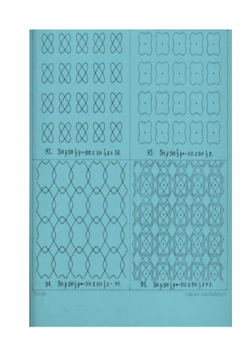
Figure 5: Part of plate showing Newton and Phillips’ Figs. 92–95, courtesy of CAAS.

Newton and Phillips recognise that the third case is a limiting special case, as can be seen from their Fig. 95, though they do not comment on that specifically in their paper. It is not clear whether they have shown, perhaps by a calculation like that in Appendix A below, the critical nature of the value $b=-7/16$, to which $b=-0.44$ is an approximation. Perhaps they have calculated this value to two decimal places by some approximation scheme, or simply by plotting examples very accurately.

Their Figs. 136–146 show the graphs in some cases with $m=1/2$ and $n=1/3$, in particular the cases with $a=1.37$ and with $b=0.60$, $b=0$ and $b=-0.77$, shown in their Figs. 144–146 and here in Fig.6.

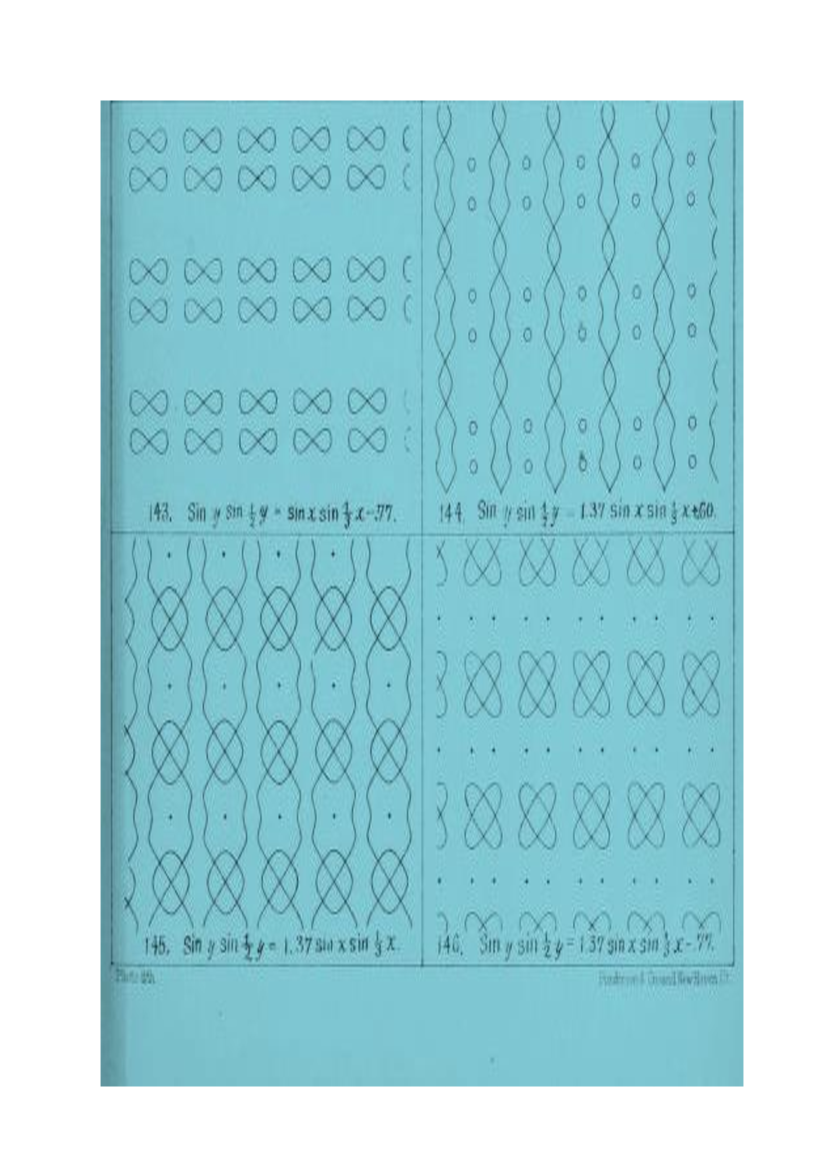
Figure 6: Part of plate showing Newton and Phillips’ Figs. 144–146, courtesy of CAAS.

Again, it is not known if the authors have carried out as in Appendix B, a calculation for the case with $b=0$ to obtain the critical value $a=64\sqrt{3}/81$, to which $a=1.37$ is an approximation, again accurate to two decimal places.

The paper of Newton and Phillips will be noted in Nature [15] and Popular Science [16], and the authors will talk separately about aspects of their work at the Detroit meeting of the AAAS later in 1875 [17, 18].

Meanwhile, across the Atlantic, 35-year-old Friedrich Wilhelm Georg Kohlrausch has just arrived in the German city of Würzburg to take up his position as Professor of Physics at JMU Würzburg. There he will continue to build an international reputation for research in electrochemistry and for the development of laboratory techniques and equipment, before moving on later to professorial positions in Strassburg in 1888 and then Berlin in 1900 [19]. He too will be elected a Foreign Member of the Royal Society of London, in 1895. His widely acclaimed textbook on the methods of experimental physics has already appeared in 1870. Translated into several languages and with many revisions, it will continue to guide beginning experimental physicists well into the 21st Century, after reaching its 24th Edition [20].

Joining Kohlrausch in Würzburg in 1875 as Research Assistant and PhD student is a brilliant young Czech, 25-year-old Vincenc (Čeněk) Strouhal from Prague, who has completed his undergraduate studies at Charles University, with Ernst Mach as one of his teachers. In 1878, Strouhal will complete a ground-breaking thesis under Kohlrausch’s guidance, on the “purring tones” that are emitted when thin stretched wires are subjected to cross-winds, leading to “vortex shedding”. His published results [21] will be extensively cited in years to come (see for example the review [22]), and the dimensionless quantity that partly characterizes the phenomenon will come to be known as the “Strouhal number”.

But in 1875, Kohlrausch has been given the challenge of designing a new physics building on land recently acquired near what is now the Röntgen Ring in Würzburg, and young Strouhal is keen to participate in the project. In Prague he has been an enthusiastic student of mathematics, becoming treasurer of the Union of Czech Mathematicians, later to become the Union of Czech Mathematicians and Physicists, and he has already presented to the Union members, when aged only 21, a series of eight talks [23] on Gauss’ famous study of curved surfaces [24].

Strouhal obtains a copy of Newton and Phillips’ paper, possibly after seeing it listed in Nature [15], where the reference to “carpet patterns” may have given him the idea to use some of the patterns in a tiled entrance to the new building. He convinces Kohlrausch to make some money available for this purpose, and chooses the two patterns shown in Newton and Phillips’ Figs. 94 and 145, essentially the same as the computer-generated figures shown in Figs. 3 and 4. As already noted, the chosen patterns correspond to two particular formulas of the form (2), the first with $m=n=1/3$, $a=-1$ and $b=-0.44$, and the second with $m=1/2$, $n=1/3$, $a=1.37$ and $b=0$.

Now Strouhal has to redraw each curve carefully, on a grid one period long, by one period wide, to define two tile-designs as clearly seen in Figs. 1 and 2. Thus each of the tiles forming the inner pattern is square, showing one period in each direction of the curves determined by the first formula, with each of $x$ and $y$ running from $-3\pi/2$ to $3\pi/2$. Similarly, each of the tiles forming the outer, edging pattern is rectangular, showing one period in each direction of the curves determined by the second formula, with $x$ running from $-3\pi/2$ to $3\pi/2$ and $y$ running from $-2\pi$ to $2\pi$. The length scales for each design are adjusted so the tiles will fit neatly together, as in Figs. 1 and 2. (The design for the corner tiles is cleverly constructed from two parts of the second pattern.)

While redrawing the curves, Strouhal notices that the critical values $b=-0.44$ for the first pattern and $a=1.37$ for the second as used by Newton and Phillips, are more accurately given by $b=-0.4375$ and $a=1.3685$. Perhaps he does the calculation of the exact values $b=-7/16$, $a=64\sqrt{3}/81$ as in Appendices A and B below, but only records the values accurate to 4 decimal places. Or perhaps he uses an approximation scheme as Newton and Phillips may have done, and determines the values more accurately than they did, but still not exactly. In truth the changes in the curves resulting from use of the exact or either choice of approximate values are almost imperceptible.

In any event, Strouhal is sufficiently pleased with his efforts to have his improved formulas fired onto tiles to accompany the two patterns, which he combines as shown in Figs. 1 and 2.

Under the supervision of the engineer, Hrn. Ubach, the tiles are suitably colored and constructed by the famous company of Villeroy and Boch in Mettlach, Germany, and then laid in the foyer of the new building, which is completed in 1879.

In 1882 Strouhal will return to Charles University in Prague as one of its founding professors of physics, and in his turn will have the opportunity to contribute to the design of a new home for his discipline. There he will continue to build his own distinguished career.

3 Concluding remarks

I have no evidence that Newton or Phillips ever learned of the tiled floor in Würzburg, through contact with Kohlrausch or Strouhal, or by some other means. But I like to imagine that well after their careers in New Haven and Prague were established, Andrew Phillips and Vincenc Strouhal met in Würzburg and admired the results of their separate endeavours as PhD students on opposite sides of the Atlantic.

Phillips died in 1915 and Strouhal in 1922, but the tiled floor, complete with Newton and Phillips’ formulas as amended by Strouhal, has survived to the present day. This is not only a testament to the handiwork of the manufacturers Villeroy and Boch under the supervision of the engineer Hrn. Ubach, but as journalist Ernst Nöth rather grandly remarked 90 years after the floor was laid [4], it also “shows that mathematical truths are not affected by the passage of generations, governments, wars and fires, even when they are trodden underfoot by students, assistants and professors over many decades” (my translation).

And I would add as a final remark: What a marvelous way to publish mathematics!

Appendix A: The first formula

It is convenient to rewrite the formulas defining the inner and outer patterns as

$$(A)\quad F(y)+H(x)-b=0\quad{\rm and}\quad(B)\quad G(y)=aH(x)\,,$$ (A1)

where

$$F(y)=\sin(y)\,\sin(y/3)\,,\quad G(y)=\sin(y)\,\sin(y/2)\,,$$

$$H(x)=\sin(x)\,\sin(x/3)\,.\qquad\qquad\qquad$$ (A2)

The graphs of the periodic functions $F$, $G$ and $H$ are shown in Fig. 7.

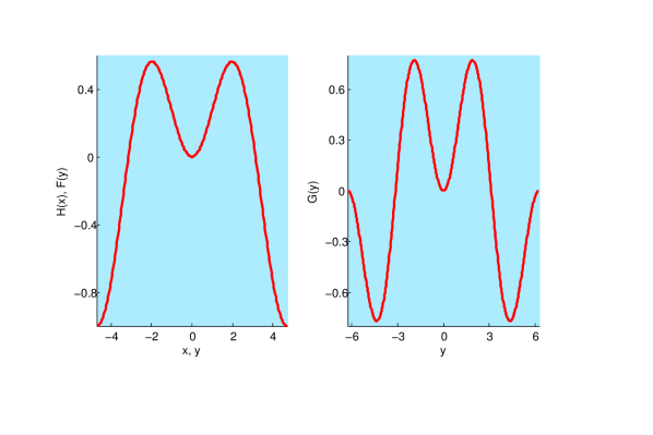
Figure 7: On the left, graph of $H(x)$ and $F(y)$ over a period from $-3\pi/2$ to $3\pi/2$. On the right, graph of G(y) over a period from $-2\pi$ to $2\pi$.

Newton and Phillips used $b=-0.44$ and $a=1.37$ to construct their Figs. 94 and 145, respectively, whereas Strouhal put $b=-0.4375$ and $a=1.3685$ in his formulas (1). Here and in Appendix B we consider slightly more general values.

If we consider a chain of figures in the $XY-$plane determined by formula $(A)$ in (A1), with $b$ values decreasing from $b=-0.40$ to $b=-0.48$ for example, as shown from L to R in Fig. 8, we see in the middle figure that the curves close to form an especially attractive pattern when $b=b_{0}\approx-0.4375\approx-0.44$, as chosen in (1) and [8]. To determine this critical value exactly, we focus attention on $b>b_{0}$ and in particular on the two points where $dy/dx=0$, at $x=x_{0}\approx 2$ and $y\approx 5$.

Figure 8: Patterns determined by Formula $(A)$ with, from L to R, $b=-0.40$, $b=-0.4375$, and $b=-0.48$.

Firstly, we find $x_{0}$ from

$$F^{\prime}(y)\,\frac{dy}{dx}=-H^{\prime}(x)=\cos(x)\,\sin(x/3)+{\textstyle\frac{1}{3}}\sin(x)\,\cos(x/3)=0\,,$$ (A3)

giving

$$3\tan(x/3)=-\tan(x)$$ (A4)

and hence, with $t=\tan(x/3)$,

$$3t=-\,(3t-t^{3})/(1-3t^{2})\,,\quad(\Rightarrow t=0,\sqrt{3/5}\quad\!\!{\rm or}\quad\!\!\!-\sqrt{3/5})\,.$$ (A5)

The root of interest is $t=\sqrt{3/5}$, giving

$$x_{0}=3\,\arctan\left(\sqrt{3/5}\right)\approx 1.9772\,.$$ (A6)

Now we find

$$H(x_{0})=\sin(x_{0}/3)\,\sin(x_{0})=s_{0}(3s_{0}-4s_{0}^{3})\,,\quad s_{0}=\sin(x_{0}/3)\,,$$ (A7)

and use $t_{0}=s_{0}/\sqrt{1-s_{0}^{2}}$ to get

$$s_{0}^{2}=t_{0}^{2}/(1+t_{0}^{2})=3/8\,,$$ (A8)

and hence

$$H(x_{0})=9/16\,.$$ (A9)

From formula $(A)$ we then have at $x=x_{0}$

$$\sin(y)\,\sin(y/3)=-\,H(x_{0})+b=\gamma,\,\,{\rm say},$$ (A10)

or

$$S\,(3S-4S^{3})=\gamma\,,\quad S=\sin(y/3)\,,$$ (A11)

implying

$$S^{2}=(3\pm\sqrt{9-16\gamma})/8\,.$$ (A12)

With $b<0$, we have $\gamma<0$ from (A9) and (A10), and it follows that only the upper sign is relevant in (A12). Because $S^{2}\leq 1$, it then follows using (A9) that

$$3+\sqrt{9-16\gamma}\leq 8\quad\left(\Rightarrow-16\gamma\leq 16\,\,\Rightarrow b\geq-7/16\right)\,.$$ (A13)

For each $b>-7/16$, it now follows that $S^{2}=\sin(y/3)^{2}<1$, leading to two possible values of $y$ with $dy/dx=0$ and with $0<y<3\pi$. But when $b=-7/16$, it follows that $y=3\pi/2$ is the only possible value in this interval. Thus the critical value $b_{0}$, when the two $y$ values with $dy/dx=0$ collapse to one, is the value given by Strouhal,

$$b_{0}=-7/16=-0.4375\,.$$ (A14)

Appendix B: The second formula

Now we consider a chain of figures determined by formula $(B)$ in (A1), with $a$ values increasing from $1.33$ to $1.41$ as shown in Fig. 9, and this time concentrate on the points near $x=2$, $y=2$ where $dy/dx=0$.

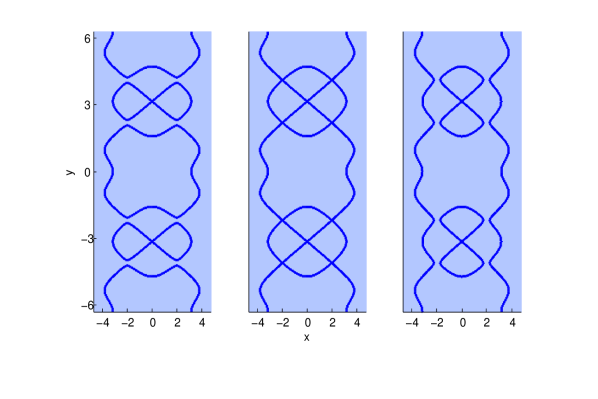
Figure 9: Patterns determined by Formula $(B)$ with, from L to R, $a=1.30$, $a=1.36853$, and $a=1.44$.

We see again a coincidence of these two points, this time when $a=a_{0}\approx 1.3685\approx 1.37$, the values chosen in (1) and [8]. To determine the exact value of $a_{0}$, we note firstly that for general $a$, the $x$-cordinate of these points is again $x=x_{0}$ as in (A6), so the $y$-coordinates of these points are determined by

$$G(y)=a\,H(x_{0})=9a/16=\tau,\,\,{\rm say}.$$ (B1)

If we consider the graph of $G(y)$ as in Fig. 7, we see that there is a single maximum in the range of $y$-values of interest (say $0<y<\pi$), occurring at a value $y=y_{0}$ to be determined. Denoting $G(y_{0})$ by $G_{{\rm max.}}$, we see that there are two roots of (B1) in the designated range provided $\tau<G_{{\rm max.}}$, and just one root if $\tau=G_{{\rm max.}}$.

To calculate $G_{{\rm max.}}$, we use

$$G^{\prime}(y)=\cos(y)\,\sin(y/2)+{\textstyle\frac{1}{2}}\sin(y)\,\cos(y/2)=0\,\,{\rm at}\,\,y=y_{0}\,,$$ (B2)

giving

$$(1-2\sigma^{2})\sigma+\sigma(1-\sigma^{2})=0\,,\quad\sigma=\sin(y_{0}/2)\,,$$ (B3)

and hence (noting the allowed range of $y$-values)

$$\sigma=\sqrt{2/3}\,.$$ (B4)

Now $\cos(y_{0}/2)=\sqrt{1-\sigma^{2}}=1/\sqrt{3}$, and hence

$$G_{{\rm max.}}=G(y_{0})=2\sin^{2}(y_{0}/2)\,\cos(y_{0}/2)=4/3\sqrt{3}\approx 0.770\,.$$ (B5)

Because the critical value of $\tau$ is given by $G_{{\rm max.}}$, it now follows from (B1) that the critical value of $a$ is given by

$$a_{0}=64\sqrt{3}/81=1.36853...$$ (B6)

Acknowledgements: My thanks to Vincent Hart, Ludvik Bass, Peter Jarvis, Gunnar Bartsch, Anja Schlömerkemper, Wolfgang Schlegel, Steve Webb, Robert Grebner and Matthias Reichling for their various inputs and encouragement.

References

- [1] Riesz, P.B., The life of Wilhelm Conrad Roentgen, Am. J. Roentgenol. 165 (1995), 1533–1537.
- [2] Bracken, A.J., The mystery of the strange formulae, Phys. World, (Oct. 2016, p. 22).
- [3] Schlegel, W., The tale of the tiles, Phys. World, (Dec. 2016, p. 21).
- [4] Nöth, E., sin x und sin y unter den Füssen, (Main-Post, Würzburg, July 2, 1971).
- [5] MATLAB (MathWorks, Natick MA, 2016).
- [6] Bartsch, G., Rätselhafte Spuren in Röntgens Labor (einBLICK, Presse-und Öffentlichkartsarbeit, JMU Würzburg), Dec. 13, 2016. http://www.presse.uni-wuerzburg.de/aktuell/einblick/einblick_archiv /ausgaben_ab_2013/ liste/page/2/zeitraum/2016/12/?tx_news_pi1 %5B controller%5D=News&cHash=59ea6b3f02997ba9c44e1fdee0f371a4
- [7] Das Fussboden-Rätsel in Röntgens Labor (Main-Post, Würzburg, Dec. 19, 2016). http://www.mainpost.de/regional/wuerzburg/Allgemeine-nicht-fachgebundene-Universitaeten-Mathematik-Mathematiker-Physik-Roentgen-Roentgen-Gedaechtnisstaette;art735,9448939
- [8] Newton, H.A. and Phillips, A.W., On the Transcendental Curves , Trans. Conn. Acad. Arts Sci. 3 (1874–1878), 97–107 (with 24 plates). http://www.biodiversitylibrary.org/item/88413#page/117/mode/1up
- [9] Phillips, Andrew W., Biography: Hubert Anson Newton, Amer. Math. Monthly 4 (no. 3) (1897), 67–71.
- [10] Gibbs, J. Willard, Memoir of Hubert Anson Newton, 1830–1896, Nat. Acad. Sc. USA.
- [11] Wright, H.P., Early ideals and their realization, in Andrew Wheeler Phillips (Tuttle, Morehouse & Taylor, New Haven, 1915), pp. 5–13. https://babel.hathitrust.org/cgi/pt?id=hvd.hn2k3q;view=1up;seq=13
- [12] Roberts, S., On three-bar motion in plane space, Proc. Lond. Math. Soc. s1–7 (1875), 15–23.
- [13] Cayley, A., On three-bar motion, Proc. Lond. Math. Soc. s1–7 (1876), 136–166.
- [14] Phillips, A.W. and Beebe, W., Graphic Algebra, or Geometrical Interpretation of the Theory of Equations of One Unknown Quantity, (H. Holt, NewYork, 1904).
- [15] Our Book Shelf, Nature 13 (no. 338) (1876), 483.
- [16] Miscellany, Popular Science Monthly 8 (1875), 121.
- [17] Newton, H.A., Algebraic curves expressed in trigonometric equations, AAAS, 24th Meeting, Detroit, Aug. 11, 1875, Amer. Chemist (Sept. 1875), 103. https://books.google.com.au/books?id=ZSSduuWOpkAC&pg=PA103
- [18] Phillips, A.W., On certain transcendental curves, AAAS, 24th Meeting, Detroit, Aug. 11, 1875, Amer. Chemist (Sept. 1875), 103. https://books.google.com.au/books?id=ZSSduuWOpkAC&pg=PA103
- [19] Goodwin, H.M. (Transl. and Ed.), Biographical sketch, in The Fundamental Laws of Electrolytic Conduction (Harper & Bros., NY, 1899), pp. 92-3. http://www.archive.org/stream /fundamentallawso00goodrich#page/92/mode/2up
- [20] Kohlrausch, F.W.G., Leitfaden der Praktische Physik (B.G. Teubner, Leipzig, 1870); Praktische Physik, 24th Ed. (Springer Vieweg, Berlin, 1996).
- [21] Strouhal, V., Über eine besondere Art der Tonerregung, Ann. d. Phys. 241 (10) (1878), 216–251.
- [22] Sarpkaya, T., Vortex-induced oscillations: a selective review, J. Appl. Mech. 46 (1979), 241–258.
- [23] Novák, V., Čeněk Strouhal, Časopis pro pěstování mathematiky a fysiky (J. for the Promotion of Mathematics and Physics) 39 (1910), 369–383.
- [24] Gauss, C.F., Disquisitiones generales circa superficies curvas (Typis Dieterichianis, Göttingen, 1828).