Uncovering quirk signal via energy loss inside tracker

Abstract

A quirk propagating through a detector is subject to the Lorentz force, a new confining gauge force, and the frictional force from ionization energy loss. At the LHC, it was found that the monojet search and the coplanar search were able to constrain such a quirk signal. Inspired by the coplanar search proposed by S. Knapen et.al. , we develop a new search that also utilizes the information of the relatively large ionization energy loss inside tracker. Our algorithm has improved efficiency in finding quirk signals with a wide oscillation amplitude. Because of our trigger strategy, the $Z(\to\nu\nu)+$jets process overlaid by pileup events is the dominant background. We find that the $\sim 100$ fb^-1 dataset at the LHC will be able to probe the colored fermion(scalar) quirks with masses up to 2.1(1.1) TeV, and the color neutral fermion(scalar) quirks with masses up to 450(150) GeV, respectively.

I Introduction

The Large Hadron Collider (LHC) has already collected tremendous data at its Run-1 and Run-2 with the center of mass energy ranging from 7 TeV to 13 TeV. However, the traditional analyses failed to find any new physics signals beyond the standard model (BSM) from those data. Yet there still exists the possibility that some new physics processes have been copiously produced at the LHC without being probed because of their non-conventional behavior. The long-lived exotic searches are receiving increased interests at the LHC Lee:2018pag ; Alimena:2019zri and some future facilities Chou:2016lxi ; Ariga:2019ufm . Many BSM scenarios, which include extra gauge symmetries (such as hidden valley models Strassler:2006im ; Cheng:2019yai ), predict exotic signals at the detector, for example, emerging jet Schwaller:2015gea , trackless jet Daci:2015hca , and soft bomb Knapen:2016hky , etc. Even though those exotic signals were overlooked by traditional searches, it does not mean that they are difficult to probe. In fact, there are already specific searches designed for emerging jet Sirunyan:2018njd and disappearing track Sirunyan:2018ldc by the CMS Collaboration. Very stringent bounds on those signals were obtained because of the low backgrounds.

Quirks are long-lived exotic particles that are charged under both the Standard Model (SM) gauge group and a new confining gauge group. The mass of the lightest quirk is much larger than the confinement scale ($\Lambda$) of the new gauge group. In this paper, we shall consider the quirk pair production signals at the LHC Okun:1980mu ; Kang:2008ea . Due to the confining gauge force, two quirks will start to oscillate after production. The typical oscillation amplitude in the center of mass frame can be estimated as

$$\ell=1_{\text{cm}}\times\Theta(\frac{1~{}\text{keV}}{\Lambda})^{2}\times\Theta(\frac{m_{\mathcal{Q}}}{100~{}\text{GeV}})~{},$$ (I.1)

where $m_{\mathcal{Q}}$ is quirk mass. Giving quirk mass around the electroweak scale, when $\Lambda\gtrsim\mathcal{O}(10)$ MeV, the confining gauge force will lead to intensive quirk oscillation. The quirk pair will lose energy quickly via photon and hidden glueball radiation. As a result, the quirk pair annihilates into the SM particles almost promptly($\ll 1$ ns). Searches for new resonances in the SM final states have been proposed to probe such quirk signals Cheung:2008ke ; Harnik:2011mv ; Fok:2011yc ; Curtin:2015jcv ; Chacko:2015fbc . For $\Lambda\in[10~{}\text{keV},10~{}\text{MeV}]$, the quirk oscillation amplitude is microscopic (undetected by the detector). Meanwhile, the glueball and photon radiations are not frequent enough so that the quirk pair can be long lived Kang:2008ea . Since the quirk pair system is electric neutral, the quirk hits on the tracker almost lie on a straight line. Those hits can be reconstructed as a single boosted charged particle with high ionization energy loss. This signal has been searched at Tevatron Abazov:2010yb . As for very small $\Lambda\lesssim\mathcal{O}(10)$ eV, the confining force becomes negligible comparing to the Lorentz force. In this case, the trajectory of each quirk is still a helix. Such signals will be constrained by heavy stable charged particle searches at the LHC CMS-PAS-EXO-16-036 ; Aaboud:2016uth ; Farina:2017cts .

This work will focus on the case with $\Lambda\sim[100~{}\text{eV}$-$10~{}\text{keV}]$, where the oscillation amplitude is macroscopic and each quirk trajectory can not be simply reconstructed as a helix. Moreover, the quirk pair can deposit only a little energy in the electromagnetic/hadronic calorimeter (ECal/HCal) within the timescale of 25 ns (which is the bunch crossing period of the LHC). Both quirks will be missed by conventional reconstructions in collider searches and will just behave as missing transverse energy. As a result, the quirk signal can be constrained only by monojet searches CMS-PAS-EXO-16-037 ; Aaboud:2016tnv ; Farina:2017cts when they are boosted by recoiling against an energetic initial state radiated jet. On the other hand, if the quirk pair is produced with little kinetic energy, the ECal or HCal is able to capture the quirk system. The quirk pair will eventually annihilate inside the calorimeter at some time when there are no active $\mathds{pp}$ collisions. Evans:2018jmd .

However, the quirk signal ($\Lambda\sim 1~{}\text{keV}$, $m\sim\mathcal{O}(100)$ GeV) could be more informative than just missing transverse energy. For a boosted quirk pair, the dominant confining force will lead to coplanar trajectories. Searching for coplanar hits in the tracker can greatly suppress the backgrounds while maintain very high signal efficiency. We further develop the coplanar quirk search as proposed in Ref. Knapen:2017kly by adding the information of ionization energy loss ($dE/dx$) inside the tracker. The $dE/dx$ of each cluster generated by the charged particles throughout the detector can be derived from the cluster charge, the average energy in creating an electron-hole pair, the density of silicon, and the thickness of each layer ATLAS:2011gea . Our method relies on the fact that quirks leave hits with relatively larger $dE/dx$ in the tracker than the SM particles Khachatryan:2016sfv . Aiming to search quirk signals with oscillation amplitude less than $\mathcal{O}(1)$ cm, the parameters in the analysis of Ref. Knapen:2017kly are chosen such that the time complexity of their algorithm is $\mathcal{O}(10^{6})$. However, this number grows as $\ell^{4}$, with $\ell$ given in Eq.(I.1). Using the information of $dE/dx$, the coplanar search algorithm can be much more efficient, especially when the oscillation amplitude exceeds $\mathcal{O}(1)$ cm. We will show later that the time complexity of our algorithm is $\mathcal{O}(10^{6})$, which, however, is insensitive to the quirk oscillation amplitude. Moreover, we find that the $Z(\to\nu\nu)+$jets process overlaid by pileup events is the dominant background since the signal is triggered by large missing transverse energy .

This paper is organized as follows. In Sec. II, we briefly discuss the theoretical frameworks for the quirk. Detailed studies on the equation of motion for quirks will be given in Sec. III. In Sec. IV, based on Monte Carlo events, we propose the method to separate the quirk signal from backgrounds. We draw the conclusion in Sec. V.

II The nature of quirks

The color neutral quirks are commonly present in many BSM models of neutral naturalness Curtin:2015bka , which are proposed to partly solve the little hierarchy problem BasteroGil:2000bw ; Bazzocchi:2012de . Such models include folded supersymmetry Burdman:2006tz ; Burdman:2008ek , quirky little Higgs Cai:2008au , twin Higgs Chacko:2005pe ; Craig:2015pha ; Serra:2019omd , minimal neutral naturalness model Xu:2018ofw , and so on, while other more general BSMs predict quirks that carry strong interaction Martin:2010kk . The quirk can be either a fermion or a scalar as well.

In this work, we will take the simplified model frameworks as benchmark. The quantum numbers of the quirks under $SU(N_{\text{IC}})\times SU_{C}(3)\times SU_{L}(2)\times U_{Y}(1)$ are given as

$$\tilde{\mathcal{D}}^{c} =\left(N_{\text{IC}},3,1,2/3\right)~{},~{}~{}$$ (II.1)

$$\tilde{\mathcal{E}}^{c} =\left(N_{\text{IC}},1,1,-2\right)~{},~{}~{}$$ (II.2)

$$\mathcal{D}^{c} =\left(N_{\text{IC}},3,1,2/3\right)~{},~{}~{}$$ (II.3)

$$\mathcal{E}^{c} =\left(N_{\text{IC}},1,1,-2\right)~{},$$ (II.4)

where we take $N_{\text{IC}}=3$ for the infracolor gauge group. $\tilde{\mathcal{D}}^{c}$ and $\tilde{\mathcal{E}}^{c}$ are spin zero particles, while $\mathcal{D}^{c}$ and $\mathcal{E}^{c}$ are fermions. The electric charges of $\tilde{\mathcal{D}}^{c}$/$\mathcal{D}^{c}$ and $\tilde{\mathcal{E}}^{c}$/$\mathcal{E}^{c}$ are $\frac{1}{3}$ and -1, respectively. However, due to the color confinement, one can observe only the quirk-quark bound state for $\tilde{\mathcal{D}}^{c}$ and $\mathcal{D}^{c}$. The probability for the quirk-quark bound state to have charge $\pm 1$ is around 30% Knapen:2017kly . Since we are interested only in quirk-quark bound states with nonzero electric charges, in the following, we will simply refer to the charge $\pm 1$ quirk-quark bound state as $\tilde{\mathcal{D}}^{c}$ or $\mathcal{D}^{c}$.

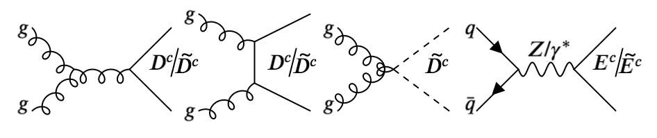
Figure 1: Production processes of quirks with different representations at the LHC.

The quirks can be pair produced at colliders through SM gauge interaction. The dominant production channels for different quirks are shown in Fig 1. The colored fermionic quirk production is given by the first two diagrams, while the colored scalar quirk receives an extra contribution from the third diagram. The color neutral quirk production is simply given by the Drell-Yan processes in the fourth diagram.

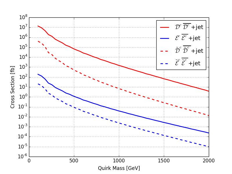
Figure 2: The leading-order production cross sections for different quirks at the 13 TeV LHC. We have also required an ISR jet with $p_{t}(\text{jet})>100$ GeV in production processes.

We also provide the production cross sections for these quirks at the 13 TeV LHC in Fig. 2. The quirk pair events with coplanar trajectories can be triggered by large missing transverse energy ($E^{\text{miss}}_{T}\gtrsim 100$ GeV CMS-PAS-EXO-16-037 ), which is induced by an energetic initial state radiation (ISR) in quirk production. So we have imposed the cut $p_{T}>100$ GeV on the ISR jet in calculating the cross sections. Because the scalar quirks have fewer degrees of freedom than the fermionic quirks and their couplings to gauge bosons are momentum suppressed, the cross sections of scalar quirks are typically more than one order of magnitude smaller than those of fermionic quirks, given the same mass and gauge group representation.

III Quirk equation of motion

The quirk equation of motion (EOM) inside the detector is given by

$$\frac{\partial(m\gamma\vec{v})}{\partial t} =\vec{F}_{s}+\vec{F}_{ext}~{},$$ (III.1)

$$\vec{F}_{s} =-\Lambda^{2}\sqrt{1-\vec{v}_{\perp}^{2}}\hat{s}-\Lambda^{2}\frac{v_{\|}\vec{v}_{\perp}}{\sqrt{1-\vec{v}_{\perp}^{2}}}~{},$$ (III.2)

$$\vec{F}_{ext} =q\vec{v}\times\vec{B}-\langle\frac{dE}{dx}\rangle\hat{v}~{},$$ (III.3)

where $v_{\|}=\vec{v}\cdot\hat{s}$ and $\vec{v}_{\perp}=\vec{v}-v_{\|}\hat{s}$ with $\hat{s}$ being a unit vector that points toward the other quirk in the center of mass frame. $\vec{F}_{s}$ corresponds to the infracolor force and is determined by the Nambu-Goto action Luscher:2002qv . $\vec{F}_{\text{ext}}$ represents the external forces, which includes the Lorentz force and the frictional force from ionization energy loss.

There are several subdominant effects that are not taken into account in the EOM. A colored quirk is surrounded by a cloud of nonperturbative QCD “brown muck” Kang:2008ea . Because of the nonperturbative QCD interaction, every time two quirks cross each other during the oscillation, a hadron with energy $\sim\Lambda_{\text{QCD}}$ will be radiated. Similarly, two quirks bound by infracolor string can emit soft infracolor glueballs with energy roughly of the order of $\Lambda$. At last, the energy loss due to Larmor radiation is proportional to $\sim\sqrt{\alpha}\Lambda\sim 0.1\Lambda$.

III.1 The $dE/dx$ inside the CMS detector

As a function of velocity in the Bethe-Bloch (BB, $\beta\gamma\gtrsim 0.06$) and Lindhard-Scharff (LS, $\beta\gamma\lesssim 0.004$) regions, the average ionization energy loss of charged particles is well predicted by the following equations Chilingarov:1999vi ; Schou:2006zz :

$$\langle\frac{dE}{dx}(v)_{\text{LS}}\rangle =A_{1}v,$$ (III.4)

$$\langle\frac{dE}{dx}(v)_{\text{BB}}\rangle =A_{2}\frac{q^{2}}{v^{2}}\ln\left(\frac{A_{3}v^{2}}{1-v^{2}}-v^{2}\right),$$ (III.5)

where the coefficients are given by

$$A_{1} =(3.1\times 10^{-11}~{}\text{GeV}^{2})\frac{\rho}{g/\text{cm}^{3}}\frac{q^{7/6}Z}{A(q^{2/3}+Z^{2/3})^{3/2}},$$

$$A_{2} =(6.03\times 10^{-18}~{}\text{GeV}^{2})\frac{\rho}{g/\text{cm}^{3}}\frac{Z}{A},$$

$$A_{3} =\frac{102200}{Z},$$

with the $A$, $Z$ and $\rho$ corresponding to the relative atomic mass, atomic number and density of material, respectively. The ionization energy loss function in the region between LS and BB is interpolated from experimental data. In a realistic measurement, the fluctuations of the ionization energy loss will follow Landau-Vavilov distribution in thick sensors Landau:1944if ; Vavilov:1957zz and Bichsel distribution in thin sensors Bichsel:1988if ; Wang:2017ygj . The thickness of tracking layers in the CMS detector ranges from 280 to 500 $\mu$m Khachatryan:2010pw , so the energy fluctuation can be well described by the Landau-Vavilov distribution. In our study, we take a Gaussian smearing on the $\langle dE/dx\rangle$ with the uncertainty about 10% for simplicity Khachatryan:2010pw .

The CMS detector uses silicon material for the tracker layers, lead tungstate (PbWO₄) for the ECal, copper for the HCal, and iron for the muon chamber. Taking parameters of materials from the Particle Data Group Tanabashi:2018oca , we plot the ionization energy loss function for the quirk propagating through each of those materials in Fig. 3. It has to be noted that the detector volume is not fully occupied. The filling rates for the tracker, ECal and HCal of the CMS detector are 0.05, 0.33 and 0.88, respectively. The ionization energy loss functions in the figure should be rescaled by the corresponding factors in solving the quirk EOM inside the CMS detector.

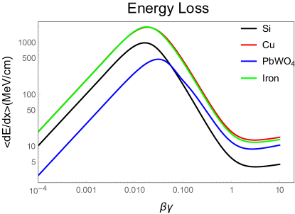
Figure 3: The ionization energy loss for charge $q=1$ particle as a function of $\beta\gamma=v/\sqrt{1-v^{2}}$ in different materials.

III.2 Numerical solution of the EOM

The tracker records the positions of quirk hits in the laboratory (lab) frame. However, the dynamics of quirk pair in the lab frame is much more difficult to describe than that in the center of mass (c.m.) frame. In the c.m. frame, the infracolor string is straight. So the direction of the $\hat{s}$ for one quirk is simply given by the relative displacement respect to the other quirk. However, the c.m. frame itself is changing all the time due to the existence of the $\vec{F}_{\text{ext}}$. Since the $\vec{F}_{\text{ext}}$ depends on the velocity of each quirk, the simultaneity and collineation of the infracolor force between two quirks in the lab frame no longer persist.

We numerically solve the quirk EOM by Euler’s method with a small time step. In the lab frame, the four-momenta of the two quirks are denoted by $(E_{i},\vec{P}_{i})$, and the space-time positions are denoted by $(t_{i},\vec{r}_{i})$ with $i=1,2$. In order to ensure the simultaneity in the c.m. frame, the following condition is required

$$t_{1}-t_{2}=\vec{\beta}\cdot(\vec{r}_{1}-\vec{r}_{2})$$ (III.6)

with $\vec{\beta}=(\vec{P}_{1}+\vec{P}_{2})/(E_{1}+E_{2})$. As a result, the time step sizes for two quirks $\epsilon_{i}(\ll 1)$ should satisfy

$$\epsilon_{1}[1- \vec{v}_{1}\cdot\vec{\beta}-\frac{\vec{r}_{1}-\vec{r}_{2}}{E_{1}+E_{2}}\cdot(\vec{F}_{1}-\vec{v}_{1}\cdot\vec{F}_{1}\vec{\beta})]=$$

$$\epsilon_{2}[1-\vec{v}_{2}\cdot\vec{\beta}-\frac{\vec{r}_{2}-\vec{r}_{1}}{E_{1}+E_{2}}\cdot(\vec{F}_{2}-\vec{v}_{2}\cdot\vec{F}_{2}\vec{\beta})],$$ (III.7)

where $\vec{F}_{i}=\vec{F}_{s,i}+\vec{F}_{ext,i}$. $\vec{F}_{s,i}$ stands for the infracolor force, and $\vec{F}_{ext,i}$ represents external force of the $i$th quirk. $\vec{v}_{i}$ is the velocity of quirk in the lab frame.

Then, for two quirks at any $(t^{\prime}_{i},\vec{r}^{\prime}_{i})$ according with the relation of Eq. (III.6), $\hat{s}_{1}$ and $\hat{s}_{2}$ in the lab frame are given by the unit vectors of

$$\vec{r}_{s1} =(\vec{r}^{\prime}_{1}-\vec{r}^{\prime}_{2})-(t^{\prime}_{1}-t^{\prime}_{2})\vec{v}^{\prime}_{1}~{},$$ (III.8)

$$\vec{r}_{s2} =(\vec{r}^{\prime}_{2}-\vec{r}^{\prime}_{1})-(t^{\prime}_{2}-t^{\prime}_{1})\vec{v}^{\prime}_{2}~{}.$$ (III.9)

To control the truncation error in the Euler’s Method, the time step sizes of two quirks should satisfy

$$\epsilon_{1,2}<10^{-4}~{}\text{ns}\frac{m_{\mathcal{Q}}}{100~{}\text{GeV}}\frac{1~{}\text{keV}^{2}}{\Lambda^{2}}.$$ (III.10)

Finally, the time evolution stops when any of the following criteria are met

• the evolution time of both quirks is longer than 25 ns, or

• both quirks are propagating outside the HCal.

III.3 Thickness of the quirk hits plane

The CMS tracker is segmented into cylindrical barrels, which surround the beam pipe, and end caps on both sides of the barrels. It consists of two subsystems: the pixel detector and the strip tracker. The details of the CMS detector parameters can be found in Ref. Chatrchyan:2008aa , and we illustrate the barrel layers in Fig. 5. In our simulation, the resolution of the hit positions in the tracker will be taken as 10 $\mu$m.

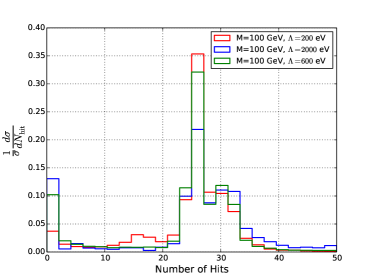
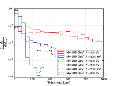
Figure 4: The distributions of the total number of hits for the quirk system traveling through the CMS tracker (upper). The distributions of the reconstructed thickness of the quirk pair plane (lower).

The charged quirks will leave a number of hits in the tracker, from which we can reconstruct the thickness of the quirk pair plane. In the upper panel in Fig. 4, we plot the distributions for the number of hits of the quirk pair with different confinement scales $\Lambda=200~{}\text{eV},~{}600~{}\text{eV}$, and $2~{}\text{keV}$. In the figure, we have chosen the quirk mass $m_{\mathcal{Q}}=100$ GeV and the transverse momentum of quirk pair $p_{T}>100$ GeV. We can find that the number of hits is weakly related to the confinement scale. Most of the events have 26 hits in the tracker because the quirk pair with large transverse momenta can go through all 13 barrel layers. There is also a great possibility that the quirk system leaves more than 26 hits inside tracker, when the quirk travels into end cap layers or the quirk crosses the same layer more than once.

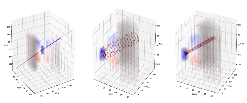
Figure 5: Trajectories of two quirks inside the CMS tracker, with the confinement scale chosen as 1 eV, 1 keV and 2 keV (from left to right). The quirk system in different panels have common initial momentum and the quirk mass is 100 GeV. The cylinder segments indicate the barrel layers.

Given a set of hit positions $\vec{h}_{i}$ ($i=1,2,\dots,N$), we can define

$$d(\vec{n})=\sqrt{\frac{1}{N-1}\sum_{i=1}^{N}(\vec{n}\cdot\vec{h}_{i})^{2}}$$ (III.11)

to describe the average distance between the hits and a virtual plane $\vec{n}$, which also includes the primary vertex. The $\vec{n}$ that gives the smallest $d(\vec{n})$ (denoted by $d_{\min}$) corresponds to the normal vector of the quirk plane. The thickness of the quirk plane is induced by the $\vec{n}$-component of the Lorentz force, so it can be estimated as Li:2020aoq

$$d_{\min}\sim 1.16\left(\frac{m}{100~{}\text{GeV}}\right)\left(\frac{\text{keV}}{\Lambda}\right)^{4}\left(\frac{|q|}{e}\right)\left(\frac{B_{xy}}{T}\right)\mu\text{m},$$ (III.12)

where $B_{xy}=|\vec{B}-(\vec{B}\cdot\vec{n})\vec{n}|$.

The thickness of the quirk plane can also be calculated by the algorithm proposed in Ref. Knapen:2017kly , which is simplified to an eigenvalue problem. We have verified that the thickness calculated from this method matches well with our estimation in Eq. (III.12). In the lower panel in Fig. 4, we plot the distributions of the quirk plane thickness, varying both the quirk mass and the confinement scale. As before, the quirk pair is required to have $p_{T}>100$ GeV in the event simulation. It is clear that the dependence on the confinement scale is much stronger than the dependence on quirk mass. We can also observe that for $\Lambda\in[\mathcal{O}(100)~{}\text{eV},\mathcal{O}(1)~{}\text{keV}]$, most of the events have a quirk plane thickness smaller than $\sim\mathcal{O}(100)~{}\mu$m. In what follows, we will focus on the case with confinement scale $\sim$ keV.

IV Signal and background analyses at the 13 TeV LHC

In the Monte Carlo simulation of event samples, the simplified models for four different quirks are implemented in FeynRules Alloul:2013bka . The general purpose event generation framework MG5_aMC@NLO Alwall:2014hca is used to simulate the quirk production processes with the model file provided by FeynRules. Then the built-in Pythia8 Sjostrand:2007gs is used for implementing the parton shower, hadronization and decay of the SM particles. However, the QCD parton shower as well as the hadronization of the colored quirk is neglected for simplicity.

Because the missing transverse energy trigger is adopted in the quirk search, the dominant background is the $Z(\to\nu\nu)+$jets process. In generating the $Z(\to\nu\nu)+$jets events, we require the transverse momentum of the $Z$ boson to be $p_{T}(Z)>200$ GeV. This is conservative, since a much stronger cut will be applied in the later analysis. The MLM prescription Hoche:2006ph is used for matching of matrix element (up to two jets) with parton showers. The events with exactly one jet in the final state are selected as in the monojet search. We also consider the background process of $Z(\to\nu\nu)e^{+}e^{-}+$ jet as pointed out in Ref. Knapen:2017kly , with $p_{T}(Z)>100$ GeV and $p_{T}(e)>1$ GeV. The production cross sections for $Z(\to\nu\nu)+$jet and $Z(\to\nu\nu)e^{+}e^{-}+$ jet after applying preliminary $p_{T}$ cuts are 3.6 pb and 13.95 fb, respectively. Note that the $W(\to\ell\nu)$+jet process can have relatively large missing transverse energy as well. However, this process can be suppressed by vetoing events that contain either an electron or muon or a reconstructed $\tau$. Only $W(\to\ell\nu)$+jet events with missing lepton and $W(\to\tau\nu)$+jet events with the hadronically decaying $\tau$ being mis-tagged as a QCD jet can survive. Its rate is much smaller than the rate of $Z(\to\nu\nu)+$jets event, so we will not consider this background.

The trajectory of a charged SM particle in the tracker is a helix, which is determined by the initial momentum of the particle. The hits of the particle can be obtained by calculating the intersecting points between the helix and the tracking layers. As for quirks, after solving the EOM numerically as discussed in Sec. III, we illustrate their trajectories inside the CMS tracker in Fig. 5. In all three panels, the quirk masses and initial momenta are fixed to the same values, while the confinement scales are chosen to be 1 eV, 1 keV and 2 keV, respectively.

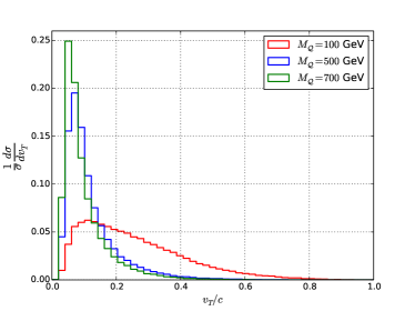
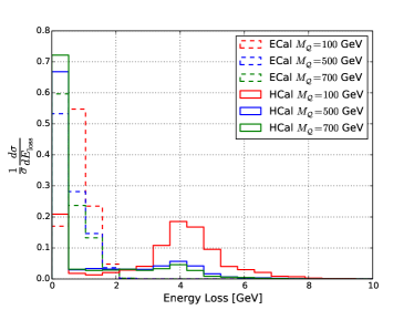
Figure 6: The distributions of transverse velocity of the quirk pair system (upper panel). The distributions of energy loss of the quirk pair in the ECal and HCal (lower panel). Three different masses of quirk have been chosen for presentation. The quirk pair is required to have $p_{T}>100$ GeV in the event simulation.

Before moving on to designing the quirk search method, we discuss a few features of the quirk’s motion in the detector. The duration of a quirk traveling inside the detector is proportional to the inverse of transverse velocity $v_{T}$ of the quirk pair system. The distribution of $v_{T}$ is shown in the upper panel in Fig. 6. Even though each quirk can have velocity $\gtrsim 0.5$, the quirk pair system is moving slowly with $v_{T}\sim 0.1$, especially when the quirk is heavy. As a result, the quirk system can escape the tracker within $10-20$ ns (given the CMS detector). While the quirk is traveling in the calorimeter, it will lose energy by ionization . According to our simulation, given $\Lambda\sim\mathcal{O}(1)~{}\text{keV}$, $m_{\mathcal{Q}}\sim\mathcal{O}(100)$ GeV, and transverse momentum of the quirk pair $p_{T}>100$ GeV, the total energy losses inside the ECal and HCal are around 1 and 4 GeV, respectively, as shown in the lower panel of the Fig. 6. It should be noted that we count only the energy deposition within the colliding period of 25 ns. According to our simulation, there are $\mathcal{O}(10)$% ($\gtrsim 50$%) of quirks that cannot reach the ECal (HCal) of the CMS detector within 25 ns. Most of the quirk pairs are still propagating in the HCal after 25 ns.

IV.1 Pileup simulation

During a bunch crossing period at the LHC, there are multiple proton-proton collisions (referred as pileup), which are dominated by the nondiffractive events (the sample is referred as the minimum bias) with small transverse momenta transfer. Pythia8 Sjostrand:2007gs adopts perturbative parton shower, Lund-string hadronization, multiple parton interaction and colour reconnection models to simulate the minimum bias. However, those models contain many parameters, which can only be deducted from experimental data. The set of chosen parameters is referred as Pythia tunes ATLAS:2012uec . The A3 tune with phenomenological parameters provided in Refs. Skands:2014pea ; ATL-PHYS-PUB-2016-017 is taken in our simulation of pileup events, because it is found to provide a good agreement with the charged particle distributions at the ATLAS detector.

The number of pileup events per bunch crossing at the LHC follows Poisson distribution with an average value around $\langle\mu\rangle\sim 30-50$. They will give $\mathcal{O}(10^{4})$ hits inside the tracker, and, thus become the main background in our analysis. In our simulation, both signal and background events are overlaid by $\langle\mu\rangle=50$ pileup events in order to draw a conservative conclusion. Moreover, due to the finite size of the beam spot, the interaction points of the pileup events could be spread along the z direction. We will assume the z coordinate of the interaction points follows a Gaussian distribution with a width of 45 mm.

The hits caused by pileup events can be obtained by the same method as has been used for the $Z+$jets background, i.e., intersecting the helix trajectories of the charged particles with the CMS tracking layers.

IV.2 Quirk signal selections

In this section, we will propose a dedicated algorithm to separate the quirk hits from the SM particle hits. In the following discussion, the quirk refers to the $\tilde{\mathcal{D}}^{c}$ and $\Lambda=1$ keV, even though our algorithm is also applicable to quirks with different quantum numbers and different values of $\Lambda$.

In searching for the quirk signals, we should first find the plane that quirks move on based on the recorded hits inside the tracker.

• First, the hits with $dE/dx$ smaller than 3.0 MeV/cm are removed to reduce the number of background hits. The quirk hits are kept intact at this stage. The remaining hits are classified according to the $dE/dx$. For each class, the average $dE/dx$ is defined as

  $$\left(\frac{dE}{dx}\right)_{\text{avg}}^{a}=\frac{1}{N_{a}}\Sigma_{i=1}^{i=N_{a}}\left(\frac{dE}{dx}\right)_{i}$$ (IV.1)

  where $N_{a}$ is the number of hits in the ath class. We loop over all the hits. A hit is assigned to the class $a$ if $|\left(\frac{dE}{dx}\right)_{\text{this hit}}-\left(\frac{dE}{dx}\right)_{\text{avg}}^{a}|<1.0~{}\text{MeV/cm}$. Otherwise, a new class is created and the hit is put into it.

  After the hit classification, the classes with fewer than 80 hits  will be used directly in step B. On the other hand, in classes with more than 80 hits, the sets of hits which belong to helix trajectories are removed. This step is found to be very useful for pileup hit removal. In practice, we will try to reconstruct the circles in the transverse plane instead of reconstructing the true helixes. The location of the center of the circle (COC) in the transverse plane for any two hits (plus the origin) is given by

  $$x_{0} =\frac{1}{2\left(k_{1}-k_{2}\right)}\left[k_{1}x_{2}\left(1+k^{2}_{2}\right)-k_{2}x_{1}\left(1+k^{2}_{1}\right)\right]~{},$$

  $$y_{0} =-\frac{x_{0}}{k_{1}}+\frac{x_{1}}{2k_{1}}+\frac{y_{1}}{2}~{},$$

  where $k_{1}=y_{1}/x_{1}$ and $k_{2}=y_{2}/x_{2}$. $x_{1},y_{1}$ and $x_{2},y_{2}$ are $x$-$y$ coordinates of the two hits. In each iteration, we pick out $80\times 80$ pairs of hits in each class randomly (even in the class with a number of hits much larger than 80). After calculating the position of the COC and the radius for each hit pair, the list of the selected hit pairs in each class is sorted by the size of the radius . Then, we compare the position of the COC and the radii of the adjacent hits. If the distance between the two COCs is smaller than 0.5 cm and the difference between the two radii is smaller than 0.1 cm , the two pairs of hits are considered to be induced by the same SM particle. Subsequently, all of the hits that lie on the circle will be removed from the class. The iteration continues until the total number of hits in all classes is less than 1500.

  	$\langle\epsilon_{1}\rangle$	$\langle\epsilon_{2}\rangle$	$\langle\epsilon_{3}\rangle$	$\langle\epsilon_{4}\rangle$	$\langle\epsilon^{1500}\rangle$
  $m_{\mathcal{Q}}=200~{}\text{GeV}$	0.965	0.590	0.5010	0.443	0.903
  $m_{\mathcal{Q}}=500~{}\text{GeV}$	0.933	0.356	0.307	0.278	0.899
  $m_{\mathcal{Q}}=800~{}\text{GeV}$	0.910	0.372	0.316	0.276	0.871
  Background	0.167	0.064	0.055	0.049	0.153

  Table 1: The average signal and background reduction efficiencies at the $i$th iteration. The last column is the average reduction efficiencies when the remaining number of hits goes below 1500.

  In Table 1, we list the average reduction efficiencies after $i$th iterations $\langle\epsilon_{i}\rangle$ and the average reduction efficiencies when the remaining number of hits is less than 1500 $\langle\epsilon^{1500}\rangle$. The reduction efficiencies for the quirk and background are defined as the ratio between the number of quirk(background) hits after the removal and the total number of quirk(background) hits. The $\langle\epsilon_{i}\rangle$ is obtained by averaging all events. We can see that one iteration can already reduce the number of hits to close to 1500 in both quirk and background events.

• Second, we should calculate the normal vector of the virtual quirk plane based on the hits after the selections in step A, which include all the hits in hit classes with fewer than 80 hits and the remaining hits in the hit classes with 80 hits or more. Assuming the origin is contained in the quirk plane, the plane normal vector can be determined for any two hits: $\vec{n}=\langle\vec{r}_{1}\times\vec{r}_{2}\rangle$, where $\vec{r}_{1}$ and $\vec{r}_{2}$ are the coordinates of the two hits. For a given plane, the distance of a new hit ($\vec{r}_{i}$) to the plane is $d_{i}=|\vec{r}_{i}\times\vec{n}|$. Our choice of $\Lambda=1$ keV leads to a typical plane thickness of $\sim\mathcal{O}(10^{-5})$ m. So we count the number of hits that are within a distance of $30~{}\mu$m to the plane. The plane  with the largest number of counted hits is kept and will be regarded as the quirk plane. In the upper panel in Fig. 7, we plot the distributions of the number of hits ($N_{\text{left}}$) within the quirk plane ($d<30~{}\mu$m) for signals with different quirk masses as well as the background. We can observe that the signals tend to have much larger number of hits than the background. Moreover, the cutoff at $N_{\text{left}}=26$ is attributed to the fact that two quirks go through all 13 barrel layers of the CMS tracker, leaving 26 hits in total.

  

  

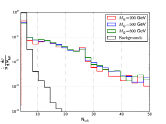
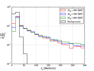
  Figure 7: The distributions for the number of hits within $d<30~{}\mu$m of the quirk plane (upper), and the distance-weighted ionization energy loss $S_{p}$ (lower).

• Third, based on the reconstructed quirk plane (with normal vector $\vec{n}_{p}$), we can define two important variables for further signal and background discrimination. The distance-weighted ionization energy loss is defined as

  $$S_{p}=\sum_{i}e^{-d_{i}/d_{0}}\times\left(\frac{dE}{dx}\right)_{i},$$ (IV.2)

  where $i$ runs over all remaining hits after step A and $d_{0}=30~{}\mu$m. Furthermore, the variation of the $S_{p}$

  $$\Delta_{p}=\max_{\Delta\theta(\vec{n}_{p},\vec{n}_{p^{\prime}})<\pi/12}\frac{|S_{p}-S_{p\prime}|}{S_{p}}$$ (IV.3)

  can also be useful for signal identification. Here, the $S_{p\prime}$ is also calculated by Eq.(IV.2), but the direction of the reference plane is varying within an angle of $\frac{\pi}{12}$ around $\vec{n}_{p}$. The distributions of $S_{p}$ for signals and background are shown in the lower panel in Fig. 7. Because of the large ionization energy loss of the quirk, the signals have significantly harder $S_{p}$ spectra than the background.

Finally, as we have discussed in Sec. IV, the large missing transverse energy ($E^{\text{miss}}_{T}$) is also an important feature of the quirk signal, so we propose the following cuts for the quirk search at the LHC:

• $E^{\text{miss}}_{T}$$\geq$ 500 GeV,

• $\Delta_{p}\geq 0.8$,

• $S_{p}\geq 50$ MeV/cm, and

• $N_{\text{left}}\geq 10$.

The cut flow of several quirk signals and backgrounds are given in Table 2, where we can find that the $E^{\text{miss}}_{T}$ cut and $S_{p}$ cut play the most important roles. .

	Quirk mass			$Zeej$	$Z+$jets
	200 GeV	400 GeV	800 GeV
$\sigma$ [fb]	33230	1484	29.92	13.95	3600
$E^{\text{miss}}_{T}\geq 500$ GeV	984	76.7	2.20	$0.02$	84.5
$\Delta_{p}\geq 0.8$	910	72.6	2.09	$0.018$	72.5
$S_{p}\geq 50$ MeV/cm	429	33.6	1.21	$\sim 0$	$0.51$
$N_{\text{left}}\geq 10$	413	28.9	1.01	$\sim 0$	$0.12$

Table 2: Cut flows of our analysis for the colored scalar quirk $\tilde{\mathcal{D}}^{c}$ pair productions and for the SM background processes. Three different masses of quirk have been chosen for illustration. The numbers in the table correspond to the cross sections (in femtobarns) at the 13 TeV LHC.

In Fig. 8, we plot the 95% confidence level (C.L.) exclusion limits for quirks with different quantum numbers at 13 TeV LHC. The search sensitivities for quirks with different quantum numbers are significantly different, attributed to two facts. Most importantly, the production cross sections of quirks are quite different as shown in Fig. 2. Moreover, quirks with different quantum numbers have different production channels, which lead to different quirk momentum distributions. The integrated luminosity at the LHC run 2 is $\sim 100$ fb^-1. It means the colored fermion(scalar) quirks with masses up to 2.1(1.1) TeV, and color neutral fermion(scalar) quirks with masses up to 450(150) GeV can be possibly probed or excluded.

Figure 8: The 95% C.L. exclusion limits for quirks with different quantum numbers at 13 TeV LHC.

V Conclusion

The quirk widely exists in new physics models with extra gauge symmetries. The color neutral quirk is well motivated by the neutral naturalness model which can solve the little hierarchy problem. We consider a simplified model framework for quirks with different quantum numbers and study their discovery prospects at the LHC.

The quirk equation of motion inside the detector is mainly controlled by the Lorentz force and the long-range infracolor force as well as the frictional force from ionization energy loss. In quirk pair production, the infracolor forces between two quirks are correlated, leading to a coupled system of nonlinear partial differential equations. It can be solved numerically in the limit that the infracolor force is much larger than the other external forces, such that the string connecting two quirks is approximately straight in the quirk pair center of mass frame. We numerically solved the full EOM for the quirk system, taking into account the architecture of the CMS detector. For the parameter space of interest [i.e. $\Lambda\sim\mathcal{O}(100-1000)$ eV, $m_{\mathcal{Q}}\sim\mathcal{O}(100)$ GeV and $p_{T}(\mathcal{Q}\bar{\mathcal{Q}})\gtrsim 100$ GeV], most of the quirk pairs can leave total number of $\sim 26$ hits inside the tracker. Those hits lie on the plane with thickness $\lesssim\mathcal{O}(100)~{}\mu$m. Meanwhile, there will be $\mathcal{O}(10)$% ($\gtrsim 50$%) of quirks that cannot reach the ECal (HCal) of the CMS detector within 25 ns (the LHC bunch spacing). The total energy losses of quirks in both the ECal and HCal within this time interval are found to be small ($\lesssim 5$ GeV).

The main background in the quirk search is the SM $Z(\to\nu\nu)$+jets process overlaid by abundant pileup events (we take $\langle\mu\rangle=50$). We propose a dedicated hit reduction algorithm to remove the SM particle hits while keeping the quirk hits as much as possible. The quirk plane is reconstructed for each event based on the selected hits. Subsequently, three discriminative variables can be defined: the number of remaining hits within a distance of $30~{}\mu$m to the quirk plane, the distance-weighted ionization energy loss in the tracker, and the variation of the $S_{p}$. Together with the missing transverse energy, they can provide a very sensitive probe for the quirk signal. With the parameters in the search optimized on the case with $\Lambda\sim 1$ keV, we find that the $\sim 100$ fb^-1 dataset at the LHC will be able to probe the colored fermion(scalar) quirks with masses up to 2.1(1.1) TeV, and color neutral fermion/scalar quirks with masses up to 450(150) GeV, respectively.

Compared to the results in Ref. Knapen:2017kly , where it predicts that the 300 fb^-1 dataset is able to probe the $\mathcal{D}^{c}$ (with $N_{\text{IC}}=2$) lighter than 1.5 TeV and the $\mathcal{E}^{c}$ (with $N_{\text{IC}}=2$) lighter than 500 GeV, the corresponding bounds for the two quirks in our analysis are 2.1 TeV and 400 GeV, respectively. There is a substantial improvement of the search sensitivity in the heavy quirk region ($m_{\mathcal{Q}}\gtrsim 1$ TeV). On the other hand, due to the stringent $E^{\text{miss}}_{T}$ cut in our analysis, the sensitivity in the light quirk region is reduced. Some cuts in our analysis should be adjusted accordingly, if one aims to search for a color neutral quirk. Moreover, the $Z(\to\nu\nu)+$jets background is not considered in Ref. Knapen:2017kly , which leads to overoptimistic results. We reproduce their analysis  and apply it to the $Z(\to\nu\nu)+$jets (overlaid by pileup events) background. We find that the efficiency for reconstructing the quirk plane that contains at least one hit in each layer in the background events is $\sim 10^{-4}$. This value is close to the efficiency of pileup background as given in Ref. Knapen:2017kly . In fact, this efficiency is dominated by the probability of finding five coplanar hits in three outer layers [up to step 2(a) in the reference], which is $\sim 10^{-3}$. Background events with five such coplanar hits usually include two charged particles flying in a similar direction. It will not be difficult to have their hits lying on a narrow strip if these two particles are energetic. Following their analysis, we find the efficiency of requiring “all but one layer must contain two hits” is $\sim 10^{-2}$. After the final selection, the cross section of $Z(\to\nu\nu)+$jets (overlaid by pileup events) is $\sim 10^{-2}$ fb, which cannot be neglected. A more detailed comparison of the sensitivities of two methods is given in the Appendix A.

Finally, let us give more comments on the ionization energy loss of quirks in the tracker. Each quirk accelerates and decelerates along its trajectory through the detector, while the quirk pair system is moving steadily with $\beta\sim 0.1$. During the oscillation, the quirk takes longer time in slower state. So there is a greater probability that the quirk crosses the tracking layers with smaller velocity, thus inducing higher ionization energy loss. It should be noted that the pattern of the ionization energy loss in different layers could be helpful for further signal and background separation Patton:2018vcl as well as quirk property characterization. We leave this for future work.

Appendix A Comparison of sensitivities

To make a comparison between the sensitivity of our method and the one proposed in Ref. Knapen:2017kly , we apply both methods to two fermionic quirks $\mathcal{D}^{c}$ and $\mathcal{E}^{c}$ , with $N_{\text{IC}}=2$ (same as in the Ref. Knapen:2017kly ). In reproducing the analysis of the Ref. Knapen:2017kly , the fiducial efficiency and the reconstruction efficiency for quirk signals are taken as 0.28 and 0.1 for simplicity. We will calculate the leading order production cross section of quirk signal after the trigger ($p_{T}>200$ GeV) by using MG5_aMC@NLO. The cross section of the $Z(\to\nu\nu)+$jets background after all of the selections is taken as $10^{-2}$ fb.

The 95% C.L exclusion limits for $\mathcal{D}^{c}$ and $\mathcal{E}^{c}$ obtained from three different methods are shown in the upper panel of the Fig. 9:

• Our method with all of the backgrounds (black lines).

• The method proposed in Ref. Knapen:2017kly without considering the $Z(\to\nu\nu)+$jets background (red lines, they are presented for validation).

• The method proposed in Ref. Knapen:2017kly with the $Z(\to\nu\nu)+$jets background (yellow lines).

When the background of $Z(\to\nu\nu)+$jets is considered, our method shows better sensitivities for both $\mathcal{D}^{c}$ and $\mathcal{E}^{c}$: the limits are reinforced by about 100-200 GeV and $\mathcal{O}(10)$ GeV for $\mathcal{D}^{c}$ and $\mathcal{E}^{c}$, respectively.

There are two points that need to be clarified: (1) our result for the $\mathcal{E}^{c}$ quirk coincides well with that in the Ref. Knapen:2017kly , i.e. without considering the $Zjj$ background, 300 fb^-1 dataset can exclude the $\mathcal{E}^{c}$ quirk with mass below 500 GeV. (2) the bound of $\mathcal{D}^{c}$ which we reproduce is much stronger than that in the Ref. Knapen:2017kly , i.e. at 300 fb^-1, the bound is 1500 GeV in the Ref. Knapen:2017kly , while it is 2050 GeV in our simulation (without considering the $Zjj$ background). This deviation may be attributed to the incorrect cross section that is used in the Ref. Knapen:2017kly for the $\mathcal{D}^{c}$. In the lower panel of the Fig. 9, we provide the leading order cross section (calculated by MG5) for quirks either with or without associating jet. We can find that the trigger efficiency ($p_{T}(j)>$200 GeV) for $\mathcal{E}^{c}$ production process is 0.1, which coincides with the number in the Table I of the Ref. Knapen:2017kly . However, for $\mathcal{D}^{c}$, Ref. Knapen:2017kly finds the trigger efficiency is 0.24 and our result shows that the cross section of $pp\to\mathcal{D}^{c}\mathcal{D}^{c}j$ is even larger than that of $pp\to\mathcal{D}^{c}\mathcal{D}^{c}$ for $m_{\mathcal{D}^{c}}>500$ GeV (which means K-factor is greater than 2).

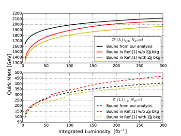
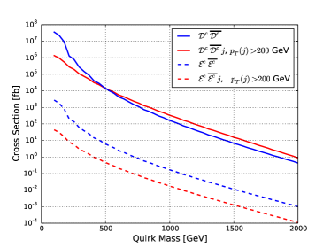
Figure 9: Upper: The 95% confident level exclusion bounds for two different fermionic quirks, from our analysis (black line), from the analysis in the Ref.[1] with (yellow line) and without (red line) considering the $Zjj$ background. Lower: the leading order production cross sections of quirk pair with and without associating jet at the 13 TeV LHC. The jet is required to have $p_{T}>$200 GeV.

References

- (1) S. Knapen, H. K. Lou, M. Papucci, and J. Setford, Tracking down Quirks at the Large Hadron Collider, Phys. Rev. D96 (2017), no. 11 115015, [arXiv:1708.02243].
- (2) L. Lee, C. Ohm, A. Soffer, and T.-T. Yu, Collider Searches for Long-Lived Particles Beyond the Standard Model, Prog. Part. Nucl. Phys. 106 (2019) 210–255, [arXiv:1810.12602].
- (3) J. Alimena et al., Searching for Long-Lived Particles beyond the Standard Model at the Large Hadron Collider, arXiv:1903.04497.
- (4) J. P. Chou, D. Curtin, and H. J. Lubatti, New Detectors to Explore the Lifetime Frontier, Phys. Lett. B767 (2017) 29–36, [arXiv:1606.06298].
- (5) FASER Collaboration, A. Ariga et al., FASER: ForwArd Search ExpeRiment at the LHC, arXiv:1901.04468.
- (6) M. J. Strassler and K. M. Zurek, Echoes of a hidden valley at hadron colliders, Phys. Lett. B651 (2007) 374–379, [hep-ph/0604261].
- (7) H.-C. Cheng, L. Li, E. Salvioni, and C. B. Verhaaren, Light Hidden Mesons through the Portal, arXiv:1906.02198.
- (8) P. Schwaller, D. Stolarski, and A. Weiler, Emerging Jets, JHEP 05 (2015) 059, [arXiv:1502.05409].
- (9) N. Daci, I. De Bruyn, S. Lowette, M. H. G. Tytgat, and B. Zaldivar, Simplified SIMPs and the LHC, JHEP 11 (2015) 108, [arXiv:1503.05505].
- (10) S. Knapen, S. Pagan Griso, M. Papucci, and D. J. Robinson, Triggering Soft Bombs at the LHC, JHEP 08 (2017) 076, [arXiv:1612.00850].
- (11) CMS Collaboration, A. M. Sirunyan et al., Search for new particles decaying to a jet and an emerging jet, JHEP 02 (2019) 179, [arXiv:1810.10069].
- (12) CMS Collaboration, A. M. Sirunyan et al., Search for disappearing tracks as a signature of new long-lived particles in proton-proton collisions at 13 TeV, JHEP 08 (2018) 016, [arXiv:1804.07321].
- (13) L. B. Okun, THETA PARTICLES, Nucl. Phys. B173 (1980) 1–12.
- (14) J. Kang and M. A. Luty, Macroscopic Strings and ’Quirks’ at Colliders, JHEP 11 (2009) 065, [arXiv:0805.4642].
- (15) K. Cheung, W.-Y. Keung, and T.-C. Yuan, Phenomenology of iquarkonium, Nucl. Phys. B811 (2009) 274–287, [arXiv:0810.1524].
- (16) R. Harnik, G. D. Kribs, and A. Martin, Quirks at the Tevatron and Beyond, Phys. Rev. D84 (2011) 035029, [arXiv:1106.2569].
- (17) R. Fok and G. D. Kribs, Chiral Quirkonium Decays, Phys. Rev. D84 (2011) 035001, [arXiv:1106.3101].
- (18) D. Curtin and C. B. Verhaaren, Quirky Explanations for the Diphoton Excess, Phys. Rev. D93 (2016), no. 5 055011, [arXiv:1512.05753].
- (19) Z. Chacko, D. Curtin, and C. B. Verhaaren, A Quirky Probe of Neutral Naturalness, Phys. Rev. D94 (2016), no. 1 011504, [arXiv:1512.05782].
- (20) D0 Collaboration, V. M. Abazov et al., Search for New Fermions (’Quirks’) at the Fermilab Tevatron Collider, Phys. Rev. Lett. 105 (2010) 211803, [arXiv:1008.3547].
- (21) CMS Collaboration Collaboration, Search for heavy stable charged particles with of 2016 data, Tech. Rep. CMS-PAS-EXO-16-036, CERN, Geneva, 2016.
- (22) ATLAS Collaboration, M. Aaboud et al., Search for heavy long-lived charged -hadrons with the ATLAS detector in 3.2 fb-1 of proton–proton collision data at TeV, Phys. Lett. B760 (2016) 647–665, [arXiv:1606.05129].
- (23) M. Farina and M. Low, Constraining Quirky Tracks with Conventional Searches, Phys. Rev. Lett. 119 (2017), no. 11 111801, [arXiv:1703.00912].
- (24) CMS Collaboration Collaboration, Search for dark matter in final states with an energetic jet, or a hadronically decaying W or Z boson using of data at , Tech. Rep. CMS-PAS-EXO-16-037, CERN, Geneva, 2016.
- (25) ATLAS Collaboration, M. Aaboud et al., Search for new phenomena in final states with an energetic jet and large missing transverse momentum in collisions at TeV using the ATLAS detector, Phys. Rev. D94 (2016), no. 3 032005, [arXiv:1604.07773].
- (26) J. A. Evans and M. A. Luty, Stopping Quirks at the LHC, JHEP 06 (2019) 090, [arXiv:1811.08903].
- (27) ATLAS Collaboration, dE/dx measurement in the ATLAS Pixel Detector and its use for particle identification, .
- (28) CMS Collaboration, V. Khachatryan et al., Search for long-lived charged particles in proton-proton collisions at 13 TeV, Phys. Rev. D94 (2016), no. 11 112004, [arXiv:1609.08382].
- (29) D. Curtin and P. Saraswat, Towards a No-Lose Theorem for Naturalness, Phys. Rev. D93 (2016), no. 5 055044, [arXiv:1509.04284].
- (30) M. Bastero-Gil, C. Hugonie, S. F. King, D. P. Roy, and S. Vempati, Does LEP prefer the NMSSM?, Phys. Lett. B489 (2000) 359–366, [hep-ph/0006198].
- (31) F. Bazzocchi and M. Fabbrichesi, Little hierarchy problem for new physics just beyond the LHC, Phys. Rev. D87 (2013), no. 3 036001, [arXiv:1212.5065].
- (32) G. Burdman, Z. Chacko, H.-S. Goh, and R. Harnik, Folded supersymmetry and the LEP paradox, JHEP 02 (2007) 009, [hep-ph/0609152].
- (33) G. Burdman, Z. Chacko, H.-S. Goh, R. Harnik, and C. A. Krenke, The Quirky Collider Signals of Folded Supersymmetry, Phys. Rev. D78 (2008) 075028, [arXiv:0805.4667].
- (34) H. Cai, H.-C. Cheng, and J. Terning, A Quirky Little Higgs Model, JHEP 05 (2009) 045, [arXiv:0812.0843].
- (35) Z. Chacko, H.-S. Goh, and R. Harnik, The Twin Higgs: Natural electroweak breaking from mirror symmetry, Phys. Rev. Lett. 96 (2006) 231802, [hep-ph/0506256].
- (36) N. Craig, A. Katz, M. Strassler, and R. Sundrum, Naturalness in the Dark at the LHC, JHEP 07 (2015) 105, [arXiv:1501.05310].
- (37) J. Serra, S. Stelzl, R. Torre, and A. Weiler, Hypercharged Naturalness, JHEP 10 (2019) 060, [arXiv:1905.02203].
- (38) L.-X. Xu, J.-H. Yu, and S.-H. Zhu, Minimal Neutral Naturalness Model, arXiv:1810.01882.
- (39) S. P. Martin, Quirks in Supersymmetry with Gauge Coupling Unification, Phys. Rev. D83 (2011) 035019, [arXiv:1012.2072].
- (40) M. Luscher and P. Weisz, Quark confinement and the bosonic string, JHEP 07 (2002) 049, [hep-lat/0207003].
- (41) A. Chilingarov, D. Lipka, J. Meyer, and T. Sloan, Displacement energy for varios ions in particle detector materials, Nucl. Instrum. Meth. A449 (2000) 277–287.
- (42) J. Schou, Slowing-down processes, energy deposition, sputtering and desorption in ion and electron interactions with solids, in CERN Accelerator School, vacuum in accelerators, Platja d’Aro, Spain, 16-24 May 2006, pp. 169–178, 2006.
- (43) L. Landau, On the energy loss of fast particles by ionization, J. Phys.(USSR) 8 (1944) 201–205.
- (44) P. V. Vavilov, Ionization losses of high-energy heavy particles, Sov. Phys. JETP 5 (1957) 749–751. [Zh. Eksp. Teor. Fiz.32,920(1957)].
- (45) H. Bichsel, Straggling in Thin Silicon Detectors, Rev. Mod. Phys. 60 (1988) 663–699.
- (46) F. Wang, S. Dong, B. Nachman, M. Garcia-Sciveres, and Q. Zeng, The Impact of Incorporating Shell-corrections to Energy Loss in Silicon, Nucl. Instrum. Meth. A899 (2018) 1–5, [arXiv:1711.05465].
- (47) CMS Collaboration, V. Khachatryan et al., CMS Tracking Performance Results from Early LHC Operation, Eur. Phys. J. C70 (2010) 1165–1192, [arXiv:1007.1988].
- (48) Particle Data Group Collaboration, M. Tanabashi et al., Review of Particle Physics, Phys. Rev. D98 (2018), no. 3 030001.
- (49) CMS Collaboration, S. Chatrchyan et al., The CMS Experiment at the CERN LHC, JINST 3 (2008) S08004.
- (50) J. Li, T. Li, J. Pei, and W. Zhang, The quirk trajectory, arXiv:2002.07503.
- (51) A. Alloul, N. D. Christensen, C. Degrande, C. Duhr, and B. Fuks, FeynRules 2.0 - A complete toolbox for tree-level phenomenology, Comput. Phys. Commun. 185 (2014) 2250–2300, [arXiv:1310.1921].
- (52) J. Alwall, R. Frederix, S. Frixione, V. Hirschi, F. Maltoni, O. Mattelaer, H. S. Shao, T. Stelzer, P. Torrielli, and M. Zaro, The automated computation of tree-level and next-to-leading order differential cross sections, and their matching to parton shower simulations, JHEP 07 (2014) 079, [arXiv:1405.0301].
- (53) T. Sjostrand, S. Mrenna, and P. Z. Skands, A Brief Introduction to PYTHIA 8.1, Comput. Phys. Commun. 178 (2008) 852–867, [arXiv:0710.3820].
- (54) S. Hoeche, F. Krauss, N. Lavesson, L. Lonnblad, M. Mangano, A. Schalicke, and S. Schumann, Matching parton showers and matrix elements, in HERA and the LHC: A Workshop on the Implications of HERA for LHC Physics: CERN - DESY Workshop 2004/2005 (Midterm Meeting, CERN, 11-13 October 2004; Final Meeting, DESY, 17-21 January 2005), pp. 288–289, 2005. hep-ph/0602031.
- (55) ATLAS Collaboration, G. Aad et al., Search for long-lived stopped R-hadrons decaying out-of-time with pp collisions using the ATLAS detector, Phys. Rev. D 88 (2013), no. 11 112003, [arXiv:1310.6584].
- (56) ATLAS Collaboration, Summary of ATLAS Pythia 8 tunes, .
- (57) P. Skands, S. Carrazza, and J. Rojo, Tuning PYTHIA 8.1: the Monash 2013 Tune, Eur. Phys. J. C74 (2014), no. 8 3024, [arXiv:1404.5630].
- (58) ATLAS Collaboration Collaboration, A study of the Pythia 8 description of ATLAS minimum bias measurements with the Donnachie-Landshoff diffractive model, Tech. Rep. ATL-PHYS-PUB-2016-017, CERN, Geneva, Aug, 2016.
- (59) S. Amrouche et al., The Tracking Machine Learning challenge : Accuracy phase, arXiv:1904.06778.
- (60) H. Patton and B. Nachman, The Optimal Use of Silicon Pixel Charge Information for Particle Identification, Nucl. Instrum. Meth. A913 (2019) 91–96, [arXiv:1803.08974].