Asymptotic profiles of the steady states for an SIS epidemic patch model with asymmetric connectivity matrix

Abstract

The dynamics of an SIS epidemic patch model with asymmetric connectivity matrix is analyzed. It is shown that the basic reproduction number $R_{0}$ is strictly decreasing with respect to the dispersal rate of the infected individuals, and the model has a unique endemic equilibrium if $R_{0}>1$. The asymptotic profiles of the endemic equilibrium for small dispersal rates are characterized. In particular, it is shown that the endemic equilibrium converges to a limiting disease-free equilibrium as the dispersal rate of susceptible individuals tends to zero, and the limiting disease-free equilibrium has a positive number of susceptible individuals on each low-risk patch. Moreover a sufficient and necessary condition is found to guarantee that the limiting disease-free equilibrium has no positive number of susceptible individuals on each high-risk patch. Our results extend earlier results for symmetric connectivity matrix, and we also partially solve an open problem by Allen et al. (SIAM J. Appl. Math., 67: 1283-1309, 2007).
Keywords: SIS epidemic patch model, asymmetric connectivity matrix, asymptotic profile
MSC 2010: 92D30, 37N25, 92D40.

1 Introduction

Various mathematical models have been proposed to describe and simulate the transmissions of infectious diseases, and the predictions provided by those models may help to prevent and control the outbreak of the diseases [5, 8, 13]. The spreading of the infectious diseases in populations depends on the spatial structure of the environment and the dispersal pattern of the populations. The impact of the spatial heterogeneity of the environment and the dispersal rate of the populations on the transmission of the diseases can be modeled in discrete-space settings by ordinary differential equation patch models [1, 6, 28, 38] or in continuous-space settings by reaction-diffusion equation models [2, 15, 40].

In a discrete-space setting, Allen et al. [1] proposed the following SIS (susceptible-infected-susceptible) epidemic patch model:

$$\begin{cases}\displaystyle\frac{d\overline{S}_{j}}{dt}=d_{S}\sum_{k\in\Omega}(\overline{L}_{jk}\overline{S}_{k}-\overline{L}_{kj}\overline{S}_{j})-\displaystyle\frac{\beta_{j}\overline{S}_{j}\overline{I}_{j}}{\overline{S}_{j}+\overline{I}_{j}}+\gamma_{j}\overline{I}_{j},&j\in\Omega,\\ \displaystyle\frac{d\overline{I}_{j}}{dt}=d_{I}\sum_{k\in\Omega}(\overline{L}_{jk}\overline{I}_{k}-\overline{L}_{kj}\overline{I}_{j})+\displaystyle\frac{\beta_{j}\overline{S}_{j}\overline{I}_{j}}{\overline{S}_{j}+\overline{I}_{j}}-\gamma_{j}\overline{I}_{j},&j\in\Omega,\end{cases}$$ (1.1)

where $\Omega=\{1,2,\dots,n\}$ with $n\geq 2$. Here $\overline{S}_{j}(t)$ and $\overline{I}_{j}(t)$ denote the number of the susceptible and infected individuals in patch $j$ at time $t$, respectively; $\beta_{j}$ denotes the rate of disease transmission and $\gamma_{j}$ represents the rate of disease recovery in patch $j$; $d_{S},d_{I}$ are the dispersal rates of the susceptible and infected populations, respectively; and $\overline{L}_{jk}\geq 0$ describes the degree of the movement of the individuals from patch $k$ to patch $j$ for $j,k\in\Omega$. A major assumption in [1] is that the matrix $(\overline{L}_{jk})$ is symmetric. In [1], the authors defined the basic reproduction number $R_{0}$ of the model (1.1); they showed that if $R_{0}<1$ the disease-free equilibrium is globally asymptotically stable, and if $R_{0}>1$ the model has a unique positive endemic equilibrium. Moreover, the asymptotic profile of the endemic equilibrium as $d_{S}\rightarrow 0$ is characterized in [1], and the case $d_{I}\rightarrow 0$ is studied in [24] recently. We remark that there are extensive studies on patch epidemic models, see [3, 14, 18, 19, 21, 26, 27, 33, 35, 38, 39] and the references therein. The corresponding reaction-diffusion model of (1.1) was studied in [2] where the dispersal of the population is modeled by diffusion. A similar model with diffusive and advective movement of the population is studied in [10, 11], and more studies on diffusive SIS models can be found in [12, 20, 23, 24, 25, 29, 30, 31, 32, 36, 42, 41] and the references therein.

The assumption that the matrix $(\overline{L}_{jk})$ is symmetric in [1, 24] is similar to the assumption of diffusive dispersal in reaction-diffusion models. However, asymmetric (e.g. advective) movements of the populations in space are common, and so in this paper we consider (1.1) with $(\overline{L}_{jk})$ being asymmetric and establish the corresponding results in [1, 24]. Moreover, we will provide solutions to some of the open problems in [1] without assuming $(\overline{L}_{jk})$ is symmetric: (1) we prove that the basic reproduction number $R_{0}$ is strictly decreasing in $d_{I}$; (2) we partially characterize the asymptotic profile of the $S$-component of the endemic equilibrium as $d_{S}\rightarrow 0$. The monotonicity of $R_{0}$ has also been proven recently in [9, 16, 17] with $\beta_{i},\gamma_{i}>0$ for all $i\in\Omega$, while this assumption will be dropped in our result. We also establish the asymptotic profile of the endemic equilibrium as $d_{I}\rightarrow 0$ when $L$ is asymmetric, which extends the results of [24] in which $L$ is assumed to be symmetric.

Denote

$$L_{jk}=\begin{cases}\overline{L}_{jk},&j\neq k,\\ -\displaystyle\sum_{k\in\Omega,k\neq j}\overline{L}_{kj},&j=k,\end{cases}$$

where $L_{jj}$ is the total degree of movement out from patch $j\in\Omega$. We rewrite (1.1) as:

$$\begin{cases}\displaystyle\frac{d\overline{S}_{j}}{dt}=d_{S}\sum_{k\in\Omega}L_{jk}\overline{S}_{k}-\displaystyle\frac{\beta_{j}\overline{S}_{j}\overline{I}_{j}}{\overline{S}_{j}+\overline{I}_{j}}+\gamma_{j}\overline{I}_{j},&j\in\Omega,\\ \displaystyle\frac{d\overline{I}_{j}}{dt}=d_{I}\sum_{k\in\Omega}L_{jk}\overline{I}_{k}+\displaystyle\frac{\beta_{j}\overline{S}_{j}\overline{I}_{j}}{\overline{S}_{j}+\overline{I}_{j}}-\gamma_{j}\overline{I}_{j},&j\in\Omega.\end{cases}$$ (1.2)

Let

$$H^{-}=\{j\in\Omega:\beta_{j}<\gamma_{j}\}\;\;\text{and}\;\;H^{+}=\{j\in\Omega:\beta_{j}>\gamma_{j}\},$$

and $H^{-}$ and $H^{+}$ are referred as the sets of patches of low-risk and high-risk, respectively. We impose the following four assumptions:

1. $\beta_{j}\geq 0$ and $\gamma_{j}\geq 0$ for all $j\in\Omega$; $d_{S},d_{I}>0$;

2. The connectivity matrix $L:=(L_{jk})$ is irreducible and quasi-positive;

3. $\overline{S}_{j}(0)\geq 0$, $\overline{I}_{j}(0)\geq 0$, and

   $$N:=\sum_{j\in\Omega}[\overline{S}_{j}(0)+\overline{I}_{j}(0)]>0;$$ (1.3)

4. $H^{-}$ and $H^{+}$ are nonempty, and $\Omega=H^{-}\cup H^{+}$.

By adding the $2n$ equations in (1.2), we see that the total population is conserved in the sense that

$$N=\sum_{j\in\Omega}\left[\overline{S}_{j}(t)+\overline{I}_{j}(t)\right]\;\;\text{for any}\;\;t\geq 0.$$ (1.4)

We remark that $(A_{0})$-$(A_{3})$ are assumed in [1] with $L$ being symmetric in addition.

Throughout the paper, we use the following notations. For $n\geq 2$,

$$\begin{split}&\mathbb{R}^{n}=\{\bm{u}=(u_{1},\dots,u_{n})^{T}:u_{i}\in\mathbb{R}\;\;\text{for any}\;\;i=1,\dots,n\},\\ &\mathbb{R}_{+}^{n}=\{\bm{u}=(u_{1},\dots,u_{n})^{T}:u_{i}\geq 0\;\;\text{for any}\;\;i=1,\dots,n\}.\end{split}$$ (1.5)

For an $n\times n$ real-valued matrix $A$, we denote the spectral bound of $A$ by

$$s(A):=\max\{\mathcal{R}e(\lambda):\lambda\;\;\text{is an eigenvalue of}\;\;A\},$$

and the spectral radius of $A$ by

$$\rho(A):=\max\{|\lambda|:\lambda\;\;\text{is an eigenvalue of}\;\;A\}.$$

The matrix $A$ is called nonnegative if all the entries of $A$ are nonnegative. The matrix $A$ is called positive if $A$ is nonnegative and nontrivial. The matrix $A$ is called zero if all the entries of $A$ are zero. The matrix $A$ is called quasi-positive (or cooperative) if all off-diagonal entries of $A$ are nonnegative.

Let $\bm{u}=(u_{1},\dots,u_{n})^{T}$ and $\bm{v}=(v_{1},\dots,v_{n})^{T}$ be two vectors. We write $\bm{u}\geq\bm{v}$ if $u_{i}\geq v_{i}$ for any $i=1,\dots,n$. We write $\bm{u}>\bm{v}$ if $u_{i}\geq v_{i}$ for any $i=1,\dots,n$, and there exists $i_{0}$ such that $u_{i_{0}}>v_{i_{0}}$. We write $\bm{u}\gg\bm{v}$ if $u_{i}>v_{i}$ for any $i=1,\dots,n$. We say $\bm{u}$ is strongly positive if $\bm{u}\gg\bm{0}$.

The rest of the paper is organized as follows. In Section 2, we prove that model (1.2)-(1.3) admits a unique endemic equilibrium if $R_{0}>1$ and prove that $R_{0}$ is strictly decreasing in $d_{I}$. In Section 3, we study the asymptotic profile of the endemic equilibrium as $d_{S}\rightarrow 0$ and $d_{I}\rightarrow 0$, and we partially solve an open problem in [1]. In Section 4, we consider an example where the patches form a star graph.

2 The basic reproduction number

In this section, we study the properties of the basic reproduction number $R_{0}$ of model (1.2). The following result on the spectral bound of the connectivity matrix $L$ follows directly from the Perron-Frobenius theorem.

Lemma 2.1.

Suppose that ($A_{1}$) holds. Then $s(L)=0$ is a simple eigenvalue of $L$ with a strongly positive eigenvector $\bm{\alpha}$, where

$$\bm{\alpha}=(\alpha_{1},\dots,\alpha_{n})^{T},\;\;\alpha_{j}>0\;\;\text{for any}\;\;j\in\Omega,\;\text{and}\;\;\sum_{i=1}^{n}\alpha_{i}=1.$$ (2.1)

Moreover, there exists no other eigenvalue of $L$ corresponding with a nonnegative eigenvector.

In the rest of the paper, we denote $\bm{\alpha}$ the positive eigenvector of $L$ as specified in Lemma 2.1.

Then we observe that model (1.2)-(1.3) admits a unique disease-free equilibrium.

Lemma 2.2.

Suppose that $(A_{0})$-$(A_{2})$ hold. Then model (1.2)-(1.3) has a unique disease-free equilibrium $(\hat{S}_{1},\dots,\hat{S}_{n},0,\dots,0)^{T}$ with $\hat{S}_{j}=\alpha_{j}N$.

Proof.

If $(\hat{S}_{1},\dots,\hat{S}_{n},0,\dots,0)^{T}$ is a disease-free equilibrium, then

$$L(\hat{S}_{1},\dots,\hat{S}_{n})^{T}=0.$$

It follows from Lemma 2.1 that there exists $\hat{k}\in\mathbb{R}$ such that $\hat{S}_{j}=\alpha_{j}\hat{k}$ for any $j\in\Omega$. Noticing that

$$\sum_{j\in\Omega}S_{j}=\hat{k}\sum_{j\in\Omega}\alpha_{j}=N,$$

we have $\hat{k}=N$. This completes the proof. ∎

We adopt the standard processes in [37] to compute the new infection and transition matrices:

$$F=diag(\beta_{j}),\;\;V=diag(\gamma_{j})-d_{I}L,$$ (2.2)

and the basic reproduction number $R_{0}$ is defined as

$$R_{0}=\rho(FV^{-1}).$$

We recall the following well-known result (see, e.g., [7, Corollary 2.1.5]):

Lemma 2.3.

Suppose that $P$ and $Q$ are $n\times n$ real-valued matrices, $P$ is quasi-positive, $Q$ is nonnegative and nonzero, and $P+Q$ is irreducible. Then, $s(P+aQ)$ is strictly increasing for $a\in(0,\infty)$.

By Lemma 2.3, if $\gamma_{j}$ ($j\in\Omega$) are not all zero, then $V$ is invertible and therefore an $M$-matrix. The following result follows from [37].

Proposition 2.4.

Suppose that $(A_{0})$-$(A_{1})$ hold and $\gamma_{j}$ ($j\in\Omega$) are not all zero. Then the following statements hold:

1. $R_{0}-1$ has the same sign as $s(F-V)=s\left(d_{I}L+diag(\beta_{j}-\gamma_{j})\right)$.

2. If $R_{0}<1$, the disease-free equilibrium $(\hat{S}_{1},\dots,\hat{S}_{n},0,\dots,0)^{T}$ of (1.2)-(1.3) is locally asymptotically stable; if $R_{0}>1$, the disease-free equilibrium is unstable.

The following result on the monotonicity of the spectral bound was proved in [9, Theorem 3.3 and 4.4], which is related Karlin’s theorem on the reduction principle in evolution biology [4, 22].

Lemma 2.5.

Suppose that $(A_{1})$ holds. Let $f_{j}\in\mathbb{R}$ for $j\in\Omega$. Then the following two statements hold:

1. If $(f_{1},\dots,f_{n})$ is a multiple of $(1,\dots,1)$, then $s\left(d_{I}L+diag(f_{j})\right)\equiv f_{1}$.

2. If $(f_{1},\dots,f_{n})$ is not a multiple of $(1,\dots,1)$, then $s\left(d_{I}L+diag(f_{j})\right)$ is strictly decreasing for $d_{I}\in(0,\infty)$.

Moreover,

$$\lim_{d_{I}\rightarrow 0}s\left(d_{I}L+diag(f_{j})\right)=\max_{j\in\Omega}f_{j},$$

and

$$\lim_{d_{I}\rightarrow\infty}s\left(d_{I}L+diag(f_{j})\right)=\sum_{j\in\Omega}f_{j}\alpha_{j}.$$

Now we prove the monotonicity of the basic reproduction number $R_{0}$ with respect to $d_{I}$. We note that this result was also proved in [16, 17] with an additional assumption $\beta_{j},\gamma_{j}>0$ for all $j\in\Omega$. If $\gamma_{j}=0$, we set $\beta_{j}/\gamma_{j}=\infty$ when $\beta_{j}>0$ and $\beta_{j}/\gamma_{j}=0$ when $\beta_{j}=0$.

Theorem 2.6.

Suppose that $(A_{0})$-$(A_{1})$ hold and $\gamma_{j}$ ($j\in\Omega$) are not all zero. Then $R_{0}$ is strictly decreasing for $d_{I}\in(0,\infty)$ if $(\beta_{1},\beta_{2},...,\beta_{n})$ is not a multiple of $(\gamma_{1},\gamma_{2},...,\gamma_{n})$.

Proof.

Clearly, $R_{0}=R_{0}(d_{I})>0$ for $d_{I}\in(0,\infty)$. We claim that

$$\min_{j\in\Omega}\displaystyle\frac{\beta_{j}}{\gamma_{j}}\leq R_{0}\leq\displaystyle\max_{j\in\Omega}\displaystyle\frac{\beta_{j}}{\gamma_{j}}.$$ (2.3)

To see this, we first assume $\gamma_{j}>0$ for all $j\in\Omega$. Then, we have $F_{1}\leq F\leq F_{2}$, where

$$F_{1}=\left(\min_{j\in\Omega}\displaystyle\frac{\beta_{j}}{\gamma_{j}}\right)diag(r_{j}),\;\;F_{2}=\left(\max_{j\in\Omega}\displaystyle\frac{\beta_{j}}{\gamma_{j}}\right)diag(r_{j}).$$

Therefore,

$$\rho(F_{1}V^{-1})\leq\rho(FV^{-1})\leq\rho(F_{2}V^{-1}),$$ (2.4)

where $F$ and $V$ are defined by (2.2). Since

$$\begin{split}&(1,\dots,1)V=(\gamma_{1},\dots,\gamma_{n}),\;\;(1,\dots,1)F_{1}=\left(\min_{j\in\Omega}\displaystyle\frac{\beta_{j}}{\gamma_{j}}\right)(\gamma_{1},\dots,\gamma_{n}),\\ &(1,\dots,1)F_{2}=\left(\max_{j\in\Omega}\displaystyle\frac{\beta_{j}}{\gamma_{j}}\right)(\gamma_{1},\dots,\gamma_{n}),\\ \end{split}$$ (2.5)

we have

$$\rho(F_{1}V^{-1})=\min_{j\in\Omega}\displaystyle\frac{\beta_{j}}{\gamma_{j}},\;\;\rho(F_{2}V^{-1})=\max_{j\in\Omega}\displaystyle\frac{\beta_{j}}{\gamma_{j}}.$$

This, together with (2.4), implies (2.3). It is not hard to check that (2.3) still holds when $\gamma_{j}\geq 0$. Indeed, if $\gamma_{j_{0}}=\beta_{j_{0}}=0$ for some ${j_{0}}\in\Omega$, the arguments above still hold as $\beta_{j_{0}}/\gamma_{j_{0}}=0$. If $\gamma_{j_{0}}=0$ and $\beta_{j_{0}}>0$ for some ${j_{0}}\in\Omega$, then $\beta_{j_{0}}/\gamma_{j_{0}}=\infty$. We can replace the $j_{0}$-th entry of $F_{1}$ by $0$ to obtain the first inequality of (2.3), and the second inequality of (2.3) is trivial.

Let

$$\mu_{0}(d_{I})=\frac{1}{R_{0}(d_{I})},$$ (2.6)

and

$$\lambda_{1}(d_{I},a):=s(-V+aF)=s\left(d_{I}L+aF-diag(\gamma_{j})\right).$$

The following discussion is divided into two cases.
Case 1. For any $a\in(0,\infty)$, $(a\beta_{1}-\gamma_{1},\dots,a\beta_{n}-\gamma_{n})$ is not a multiple of $(1,\dots,1)$. Then we see from Lemma 2.5 that for any fixed $a>0$, $\lambda_{1}(d_{I},a)$ is strictly decreasing for $d_{I}\in(0,\infty)$. Let $\phi>0$ be the corresponding eigenvector of $V^{-1}F$ with respect to $\rho(V^{-1}F)$. Then

$$d_{I}L\phi-diag(\gamma_{j})\phi+\mu_{0}(d_{I})F\phi=0.$$

Since $L$ is irreducible, it follows that $\phi\gg 0$ and $\lambda_{1}(d_{I},\mu_{0}(d_{I}))=0$ for any $d_{I}>0$. Let $d_{I}^{1}>d_{I}^{2}$. Then

$$\begin{split}&\lambda_{1}\left(d_{I}^{2},\mu_{0}\left(d_{I}^{1}\right)\right)-\lambda_{1}\left(d_{I}^{2},\mu_{0}\left(d_{I}^{2}\right)\right)\\ =&\lambda_{1}\left(d_{I}^{2},\mu_{0}\left(d_{I}^{1}\right)\right)-\lambda_{1}\left(d_{I}^{1},\mu_{0}\left(d_{I}^{1}\right)\right)>0,\end{split}$$ (2.7)

which implies that

$$\mu_{0}\left(d_{I}^{1}\right)>\mu_{0}\left(d_{I}^{2}\right),$$

and consequently, $\mu_{0}(d_{I})$ is strictly increasing for $d_{I}\in(0,\infty)$.
Case 2. There exists $\tilde{a}>0$ such that $(\tilde{a}\beta_{1}-\gamma_{1},\dots,\tilde{a}\beta_{n}-\gamma_{n})$ is a multiple of $(1,\dots,1)$. That is, there exists $k\in\mathbb{R}$ such that

$$(\tilde{a}\beta_{1}-\gamma_{1},\dots,\tilde{a}\beta_{n}-\gamma_{n})=k(1,\dots,1).$$

Clearly, $\tilde{a}$ is unique and $k\neq 0$ if $(\beta_{1},\beta_{2},...,\beta_{n})$ is not a multiple of $(\gamma_{1},\gamma_{2},...,\gamma_{n})$.

If $k>0$, then $\beta_{j}>0$ for all $j\in\Omega$ and

$$R_{0}\geq\displaystyle\min_{j\in\Omega}\displaystyle\frac{\beta_{j}}{\gamma_{j}}>\displaystyle\frac{1}{\tilde{a}},$$

which implies that $\mu_{0}(d_{I})<\tilde{a}$ for any $d_{I}>0$. Similar to Case 1, it follows from Lemma 2.5 that $\lambda_{1}(d_{I},a)$ is strictly decreasing for $d_{I}\in(0,\infty)$ for any fixed $a<\tilde{a}$. Therefore, (2.7) holds, and $\mu_{0}(d_{I})$ is strictly increasing for $d_{I}\in(0,\infty)$.

If $k<0$, then $\gamma_{j}>0$ for all $j\in\Omega$ and

$$R_{0}\leq\displaystyle\max_{j\in\Omega}\displaystyle\frac{\beta_{j}}{\gamma_{j}}<\displaystyle\frac{1}{\tilde{a}},$$

which implies that $\mu_{0}(d_{I})>\tilde{a}$ for any $d_{I}>0$. The rest of the proof is similar to the case of $k>0$. ∎

Then we compute the limits of $R_{0}$ as $d\to 0$ or $d\to\infty$.

Theorem 2.7.

Suppose that $(A_{0})$-$(A_{1})$ hold and $\gamma_{j}$ ($j\in\Omega$) are not all zero. Then the basic reproduction number $R_{0}=R(d_{I})$ satisfies the following:

$$\lim_{d_{I}\to 0}R_{0}(d_{I})=\displaystyle\max_{j\in\Omega}\displaystyle\frac{\beta_{j}}{\gamma_{j}}\;\;\text{and}\;\;\lim_{d_{I}\to\infty}R_{0}(d_{I})=\frac{\sum_{j\in\Omega}\alpha_{j}\beta_{j}}{\sum_{j\in\Omega}\alpha_{j}\gamma_{j}}.$$

Remark 2.8.

If $L$ is symmetric, then

$$\lim_{d_{I}\to\infty}R_{0}(d_{I})=\frac{\sum_{j\in\Omega}\beta_{j}}{\sum_{j\in\Omega}\gamma_{j}}.$$

as $\alpha_{j}\equiv 1/n$.

Proof.

Let $\mu_{0}(d_{I})$ and $\lambda_{1}(d_{I},a)$ be defined as in the proof of Theorem 2.6. Noticing that $\mu_{0}(d_{I})$ is increasing in $d_{I}$, let

$$\mu_{1}=\lim_{d_{I}\to 0}\mu_{0}(d_{I})\ \ \text{and }\ \ \mu_{2}=\lim_{d_{I}\to\infty}\mu_{0}(d_{I}),$$

where $\mu_{1}\in[0,\infty)$ and $\mu_{2}\in(0,\infty]$. By Lemma 2.5, for any $a>0$,

$$\lim_{d_{I}\to 0}\lambda_{1}(d_{I},a)=\max_{j\in\Omega}\{a\beta_{j}-\gamma_{j}\}\ \ \text{and }\ \ \lim_{d_{I}\to\infty}\lambda_{1}(d_{I},a)=\sum_{j\in\Omega}(a\beta_{j}-\gamma_{j})\alpha_{j}.$$ (2.8)

Since $\lambda_{1}\left(d_{I},\mu_{0}\left(d_{I}\right)\right)=0$, we have

$$\max_{j\in\Omega}\{\mu_{1}\beta_{j}-\gamma_{j}\}=0\ \ \text{and }\ \ \sum_{j\in\Omega}(\mu_{2}\beta_{j}-\gamma_{j})\alpha_{j}=0.$$ (2.9)

Indeed, to see the first equality, for given $\epsilon>0$ there exists $\hat{d}_{I}>0$ such that $\mu_{1}-\epsilon<\mu_{0}(d_{I})<\mu_{1}+\epsilon$ for all $d_{I}<\hat{d}_{I}$. By Lemma 2.3, we have

$$\lambda_{1}\left(d_{I},\mu_{1}-\epsilon\right)<\lambda_{1}\left(d_{I},\mu_{0}\left(d_{I}\right)\right)=0<\lambda_{1}\left(d_{I},\mu_{1}+\epsilon\right)\ \ \text{for all }d_{I}<\hat{d}_{I}.$$

By (2.8), we have

$$\max_{j\in\Omega}\{(\mu_{1}-\epsilon)\beta_{j}-\gamma_{j}\}\leq 0\leq\max_{j\in\Omega}\{(\mu_{1}+\epsilon)\beta_{j}-\gamma_{j}\}.$$

Since $\epsilon>0$ is arbitrary, we obtain the first equality. The other equality in (2.9) can be proved similarly.

It follows from (2.9) that

$$\lim_{d_{I}\to 0}R_{0}(d_{I})\geq\displaystyle\max_{j\in\Omega}\displaystyle\frac{\beta_{j}}{\gamma_{j}}\;\;\text{and}\;\;\lim_{d_{I}\to\infty}R_{0}(d_{I})=\frac{\sum_{j\in\Omega}\alpha_{j}\beta_{j}}{\sum_{j\in\Omega}\alpha_{j}\gamma_{j}},$$

where the equality holds for $d_{I}\to 0$ if there exists no $j\in\Omega$ such that $\beta_{j}=\gamma_{j}=0$. Noticing (2.3), the proof is complete. ∎

3 The endemic equilibrium

In this section, we consider the endemic equilibrium of model (1.2)-(1.3). The equilibria of (1.2)-(1.3) satisfy

$$\begin{cases}d_{S}\displaystyle\sum_{k\in\Omega}L_{jk}S_{k}-\displaystyle\frac{\beta_{j}S_{j}I_{j}}{S_{j}+I_{j}}+\gamma_{j}S_{j}=0,&j\in\Omega,\\ d_{I}\displaystyle\sum_{k\in\Omega}L_{jk}I_{k}+\displaystyle\frac{\beta_{j}S_{j}I_{j}}{S_{j}+I_{j}}-\gamma_{j}I_{j}=0,&j\in\Omega,\\ \displaystyle\sum_{j\in\Omega}(S_{j}+I_{j})=N.\end{cases}$$ (3.1)

Firstly, we study the existence and uniqueness of the endemic equilibrium. Then, we investigate the asymptotic profile of the endemic equilibrium as $d_{S}\rightarrow 0$ and/or $d_{I}\rightarrow 0$.

3.1 The existence and uniqueness

In this section, we show that (1.2)-(1.3) has a unique endemic equilibrium if $R_{0}>1$. Motivated by [1], we first introduce an equivalent problem of (3.1).

Lemma 3.1.

Suppose that $(A_{0})$-$(A_{3})$ hold. Then $(S_{1},\dots,S_{n},I_{1},\dots,I_{n})^{T}$ is a non-negative solution of (3.1) if and only if

$$(S_{1},\dots,S_{n},I_{1},\dots,I_{n})=\left(\kappa\check{S}_{1},\dots,\kappa\check{S}_{n},\displaystyle\frac{\kappa}{d_{I}}\check{I}_{1},\dots,\displaystyle\frac{\kappa}{d_{I}}\check{I}_{n}\right),$$

where $(\check{S}_{1},\dots,\check{S}_{n},\check{I}_{1},\dots,\check{I}_{n})$ satisfies

$$\begin{cases}d_{S}\check{S}_{j}+\check{I}_{j}=\alpha_{j},&j\in\Omega,\\ d_{I}\displaystyle\sum_{k\in\Omega}L_{jk}\check{I}_{k}+\check{I}_{j}\left(\beta_{j}-\gamma_{j}-\displaystyle\frac{d_{S}\beta_{j}\check{I}_{j}}{d_{I}(\alpha_{j}-\check{I}_{j})+d_{S}\check{I}_{j}}\right)=0,&j\in\Omega,\\ \end{cases}$$ (3.2)

and

$$\kappa=\displaystyle\frac{d_{I}N}{\displaystyle\sum_{j\in\Omega}(d_{I}\check{S}_{j}+\check{I}_{j})}.$$ (3.3)

Proof.

Clearly, from (3.1), we have

$$\sum_{k\in\Omega}L_{jk}\left(d_{S}S_{k}+d_{I}I_{k}\right)=0\;\;\text{for any}\;\;j\in\Omega.$$

Then it follows from Lemma 2.1 that there exists $\kappa>0$ such that

$$d_{S}S_{j}+d_{I}I_{j}=\kappa\alpha_{j}\;\;\text{for any}\;\;j\in\Omega.$$ (3.4)

Let

$$\check{S}_{j}=\displaystyle\frac{S_{j}}{\kappa},\;\;\check{I}_{j}=\displaystyle\frac{d_{I}I_{j}}{\kappa}.$$ (3.5)

Then

$$d_{S}\check{S}_{j}+\check{I}_{j}=\alpha_{j}\;\;\text{for any}\;\;j\in\Omega.$$

Plugging (3.4)-(3.5) into the second equation of (3.1), we see that $\check{I}_{j}$ satisfies the second equation of (3.2). Since

$$N=\sum_{j\in\Omega}(S_{j}+I_{j})=\kappa\sum_{j\in\Omega}\left(\check{S}_{j}+\displaystyle\frac{\check{I}_{j}}{d_{I}}\right),$$

(3.3) holds. This completes the proof. ∎

From Lemma 3.1, to analyze the solutions of (3.2), we only need to consider the equations of $\check{I}_{j}$ in (3.2). We consider an auxiliary problem of (3.2).

Lemma 3.2.

Suppose that $(A_{0})$-$(A_{3})$ hold and $R_{0}>1$. Then, for any $d>0$, the following equation

$$\begin{cases}d_{I}\displaystyle\sum_{k\in\Omega}L_{jk}\check{I}_{k}+\check{I}_{j}\left(\beta_{j}-\gamma_{j}-\displaystyle\frac{\beta_{j}\check{I}_{j}}{d(\alpha_{j}-\check{I}_{j})+\check{I}_{j}}\right)=0,&j\in\Omega,\\ 0\leq\check{I}_{j}\leq\alpha_{j},&j\in\Omega,\end{cases}$$ (3.6)

admits exactly one non-trivial solution $\bm{\check{I}}=(\check{I}_{1},\dots,\check{I}_{n})^{T}$, where $0<\check{I}_{j}<\alpha_{j}$ for any $j\in\Omega$. Moreover, $\check{I}_{j}$ is monotone increasing in $d\in(0,\infty)$ for any $j\in\Omega$.

Proof.

Since $R_{0}>1$, $s\left(d_{I}L+diag(\beta_{j}-\gamma_{j})\right)>0$. Let

$$f_{j}(\check{I}_{j})=\check{I}_{j}\left(\beta_{j}-\gamma_{j}-\displaystyle\frac{\beta_{j}\check{I}_{j}}{d(\alpha_{j}-\check{I}_{j})+\check{I}_{j}}\right),$$ (3.7)

and consider the following problem

$$\frac{d\bar{I}_{j}}{dt}=d_{I}\sum_{k\in\Omega}L_{jk}\bar{I}_{k}+f_{j}(\bar{I}_{j}),\;\;j\in\Omega,\;\;t>0.$$ (3.8)

Let $\bm{g}(\bm{\check{I}})=\left(g_{1}(\bm{\check{I}}),\dots,g_{n}(\bm{\check{I}})\right)^{T}$ be the vector field corresponding to the right hand side of (3.8), and let

$$U=\{\bm{\check{I}}=\left(\check{I}_{1},\dots,\check{I}_{n}\right)^{T}\in\mathbb{R}^{n}:0\leq\check{I}_{j}\leq\alpha_{j},\;j\in\Omega\}.$$

Then $U$ is positive invariant with respect to (3.8), and for any $\bm{\check{I}}\in U$,

$$D_{\bm{\check{I}}}\bm{g}(\bm{\check{I}})=d_{I}L+diag(f^{\prime}_{j}(\check{I}_{j})),$$

which is irreducible and quasi-positive. Let $\Psi_{t}$ be the semiflow induced by (3.8). By [34, Theorem B.3], $\Psi_{t}$ is strongly positive and monotone.

For any $\lambda\in(0,1)$ and $\check{I}_{j}\in(0,\alpha_{j}]$, we have

$$\begin{split}f_{j}(\lambda\check{I}_{j})-\lambda f(\check{I}_{j})=&-\displaystyle\frac{\lambda^{2}\beta_{j}\check{I}_{j}^{2}}{d(\alpha_{j}-\lambda\check{I}_{j})+\lambda\check{I}_{j}}+\displaystyle\frac{\lambda\beta_{j}\check{I}_{j}^{2}}{d(\alpha_{j}-\check{I}_{j})+\check{I}_{j}}\\ =&\displaystyle\frac{d\lambda\alpha_{j}\beta_{j}\check{I}_{j}^{2}(1-\lambda)}{[d(\alpha_{j}-\lambda\check{I}_{j})+\lambda\check{I}_{j}][d(\alpha_{j}-\check{I}_{j})+\check{I}_{j}]}\geq 0,\end{split}$$ (3.9)

and the strict inequality holds for at least one $j$. This implies that $\bm{g}(\bm{\check{I}})$ is strictly sublinear on $U$ (see [44] for the definition of strictly sublinear functions). Noticing $s\left(d_{I}L+diag(\beta_{j}-\gamma_{j})\right)>0$, it follows from [43, Theorem 2.3.4] (or [44, Corollary 3.2]) that there exists a unique $\bm{\check{I}}\gg\bm{0}$ in $U$ such that every solution in $U\setminus\{\bm{0}\}$ converges to $\bm{\check{I}}$. Moreover, if $\check{I}_{j}=\alpha_{j}$ for some $j\in\Omega$, then $\check{I}^{\prime}_{j}\leq-\gamma_{j}<0$, which implies that $\check{I}_{j}\in(0,\alpha_{j})$ for any $j\in\Omega$.

Suppose $d_{1}>d_{2}$. Let $\bm{\check{I}}^{(i)}=(\check{I}_{1}^{(i)},\dots,\check{I}_{n}^{(i)})^{T}$ be the unique strongly positive solution of (3.6) with $d=d_{i}$ for $i=1,2$, and let $\bm{\bar{I}}^{(i)}(t)=(\bar{I}_{1}^{(i)}(t),\dots,\bar{I}_{n}^{(i)}(t))^{T}$ be the solution of (3.8) with $d=d_{i}$ for $i=1,2$, and $\bm{\bar{I}}^{(1)}(0)=\bm{\bar{I}}^{(2)}(0)\in U\setminus\{\bm{0}\}$. Then for any $j\in\Omega$,

$$\begin{split}\displaystyle\frac{d\bar{I}_{j}^{(1)}}{dt}=&d_{I}\sum_{k\in\Omega}L_{jk}\bar{I}_{k}^{(1)}+\bar{I}^{(1)}_{j}\left(\beta_{j}-\gamma_{j}-\displaystyle\frac{\beta_{j}\bar{I}^{(1)}_{j}}{d_{1}(\alpha_{j}-\bar{I}^{(1)}_{j})+\bar{I}^{(1)}_{j}}\right)\\ \geq&d_{I}\sum_{k\in\Omega}L_{jk}\bar{I}_{k}^{(1)}+\bar{I}^{(1)}_{j}\left(\beta_{j}-\gamma_{j}-\displaystyle\frac{\beta_{j}\bar{I}^{(1)}_{j}}{d_{2}(\alpha_{j}-\bar{I}^{(1)}_{j})+\bar{I}^{(1)}_{j}}\right).\end{split}$$ (3.10)

It follows from the comparison principle that $\bar{I}_{j}^{(1)}(t)\geq\bar{I}_{j}^{(2)}(t)$ for any $t\geq 0$ and $j\in\Omega$. Therefore, $\check{I}_{j}^{(1)}=\displaystyle\lim_{t\to\infty}\bar{I}_{j}^{(1)}(t)\geq\check{I}_{j}^{(2)}=\displaystyle\lim_{t\to\infty}\bar{I}_{j}^{(2)}(t)$ for any $j\in\Omega$. ∎

Lemma 3.2 was proved in [1] when $L$ is symmetric by virtue of the upper and lower solution method. Here we prove it without assuming the symmetry of $L$ by the monotone dynamical system method.

By Lemmas 3.1-3.2, we can show that model (1.2)-(1.3) has a unique endemic equilibrium if $R_{0}>1$.

Theorem 3.3.

Suppose that $(A_{0})$-$(A_{3})$ hold and $R_{0}>1$. Then (1.2)-(1.3) has exactly two non-negative equilibria: the disease-free equilibrium and the endemic equilibrium

$$(S_{1},\dots,S_{n},I_{1},\dots,I_{n})=\left(\kappa\check{S}_{1},\dots,\kappa\check{S}_{n},\displaystyle\frac{\kappa\check{I}_{1}}{d_{I}},\dots,\displaystyle\frac{\kappa\check{I}_{n}}{d_{I}}\right),$$ (3.11)

where

$$\check{S}_{j}=\displaystyle\frac{\alpha_{j}-\check{I}_{j}}{d_{S}},\;\;\kappa=\displaystyle\frac{d_{I}N}{\displaystyle\sum_{j\in\Omega}(d_{I}\check{S}_{j}+\check{I}_{j})},$$ (3.12)

and $(\check{I}_{1},\dots,\check{I}_{n})^{T}$ is the unique strongly positive solution of (3.6) with $d:={d_{I}}/{d_{S}}$.

Proof.

This result follows from Lemmas 3.1–3.2. ∎

3.2 Asymptotic profile with respect to $d_{S}$

In this subsection, we study the asymptotic profile of the endemic equilibrium of (1.2)-(1.3) as $d_{S}\to 0$. We suppose that $(A_{0})$-$(A_{3})$ hold throughout this subsection. Moreover, we observe that $R_{0}$ is independent of $d_{S}$. Therefore, we assume $R_{0}>1$ throughout this subsection so that the endemic equilibrium exists for all $d_{S}>0$.

We first study the asymptotic profile of $\kappa$ and $I_{j}$, where $\kappa$ and $I_{j}$ are defined in Theorem 3.3.

Lemma 3.4.

As $d_{S}\to 0$, $\kappa\to 0$ and $I_{j}\to 0$ for any $j\in\Omega$.

Proof.

For any sequence $\{d_{S}^{(m)}\}_{m=1}^{\infty}$ such that $\displaystyle\lim_{m\to\infty}d_{S}^{(m)}=0$, we denote the corresponding endemic equilibrium by $(S^{(m)}_{1},\dots,S^{(m)}_{n},I^{(m)}_{1},\dots,I^{(m)}_{n})$. Since $I^{(m)}_{j}\in(0,N]$, there exists a subsequence $\{d_{S}^{(m_{l})}\}_{l=1}^{\infty}$ such that $\displaystyle\lim_{l\to\infty}I_{j}^{(m_{l})}=I^{*}_{j}$ for some $I^{*}_{j}\in[0,N]$. For $j\in H^{-}$,

$$d_{S}^{(m_{l})}\sum_{k\in\Omega}L_{jk}S^{(m_{l})}_{k}\leq I_{j}^{(m_{l})}(\beta_{j}-\gamma_{j})\leq 0.$$

Since $S^{(m_{l})}_{k}\in(0,N]$ for any $l\geq 1$ and $k\in\Omega$, we have

$$\lim_{l\to\infty}d_{S}^{(m_{l})}\sum_{k\in\Omega}L_{jk}S^{(m_{l})}_{k}=0,$$

which implies $I_{j}^{*}=0$. Therefore $I_{j}\to 0$ as $d_{S}\to 0$ for $j\in H^{-}$.

Since

$$d_{S}S_{j}+d_{I}I_{j}=\kappa\alpha_{j}\;\;\text{for any}\;\;j\in\Omega,$$

and $H^{-}\neq\emptyset$ by $(A_{3})$, we have $\kappa\to 0$ as $d_{S}\to 0$. This in turn implies that for $j\in H^{+}$,

$$I_{j}=\displaystyle\frac{\kappa\alpha_{j}-d_{S}S_{j}}{d_{I}}\to 0\;\;\text{as}\;\;d_{S}\to 0.$$

∎

Lemma 3.5.

For each $j\in\Omega$, $\check{I}_{j}$ is monotone decreasing in $d_{S}\in(0,\infty)$ and $\displaystyle\lim_{d_{S}\to 0}\check{I}_{j}=\check{I}_{j}^{*}\in(0,\alpha_{j}].$

Proof.

We notice that $(\check{I}_{j})$ is the positive solution of (3.6) with $d=d_{I}/d_{S}$. By Lemma 3.2, $\check{I}_{j}$ is monotone increasing in $d$, which implies that $\check{I}_{j}$ is monotone decreasing in $d_{S}$ for each $j\in\Omega$. Since $\check{I}_{j}\in(0,\alpha_{j})$ from Lemma 3.1, we have $\displaystyle\lim_{d_{S}\to 0}\check{I}_{j}=\check{I}_{j}^{*}\in(0,\alpha_{j}].$ ∎

From Lemma 3.5, we denote

$$J^{-}=\{j\in\Omega:0<\check{I}_{j}^{*}<\alpha_{j}\},\;\;\text{and}\;\;J^{+}=\{j\in\Omega:\check{I}^{*}_{j}=\alpha_{j}\}.$$ (3.13)

Clearly $\Omega=J^{-}\cup J^{+}$. We show that $J^{-}$ is nonempty.

Lemma 3.6.

$J^{-}$ is nonempty, and $H^{-}\subset J^{-}$.

Proof.

Suppose that there exists $j\in\Omega$ such that $\beta_{j}-\gamma_{j}<0$ and $\check{I}_{j}^{*}=\alpha_{j}$. By (3.6), we have

$$d_{I}\sum_{k\in\Omega}L_{jk}\check{I}_{k}+\check{I}_{j}(\beta_{j}-\gamma_{j})\geq 0.$$

Taking $d_{S}\to 0$ on both sides, we have

$$d_{I}\sum_{k\neq j,k\in\Omega}L_{jk}\check{I}_{k}^{*}+d_{I}L_{jj}\alpha_{j}\geq\alpha_{j}(\gamma_{j}-\beta_{j})>0.$$ (3.14)

Since

$$d_{I}\sum_{k\neq j,k\in\Omega}L_{jk}\alpha_{k}+d_{I}L_{jj}\alpha_{j}=0,$$

and $\check{I}_{j}^{*}\in(0,\alpha_{j}]$ for any $j\in\Omega$, we have

$$d_{I}\sum_{k\neq j,k\in\Omega}L_{jk}\check{I}_{k}^{*}+d_{I}L_{jj}\alpha_{j}\leq 0,$$

which contradicts with (3.14). Therefore, $H^{-}\subset J^{-}$. ∎

By virtue of the above lemma, we can prove the following result about the asymptotic profile of $S_{j}$. The proof is similar to [1, Lemma 4.4], and we omit it here.

Lemma 3.7.

Let $J^{-}$ be defined as above. Then

1. $\displaystyle\lim_{d_{S}\to 0}\frac{\kappa}{d_{S}}=\displaystyle\frac{N}{\displaystyle\sum_{k\in J^{-}}(\alpha_{k}-\check{I}_{k}^{*})}$;

2. For any $j\in\Omega$, $\displaystyle\lim_{d_{S}\to 0}S_{j}=\displaystyle\frac{N}{\displaystyle\sum_{k\in J^{-}}(\alpha_{k}-\check{I}_{k}^{*})}(\alpha_{j}-\check{I}_{j}^{*})$.

Similar to [1, Lemma 4.5], we can prove that $J^{+}$ is nonempty.

Lemma 3.8.

$J^{+}$ is nonempty.

For some further analysis of $J^{+}$ with respect to $d_{I}$, we define

$$M=\left(M_{jk}\right)_{j,k\in H^{-}},\;\;\text{where}\;\;M_{jk}=\begin{cases}-d_{I}L_{jk},&j,k\in H^{-},\;j\neq k,\\ -d_{I}L_{jj}-(\beta_{j}-\gamma_{j}),&j,k\in H^{-},\;j=k,\end{cases}$$ (3.15)

Then $M$ is an $M$-matrix, and $M^{-1}$ is positive. Therefore, the following system

$$-d_{I}\sum_{k\in H^{-}}L_{jk}I_{k}-(\beta_{j}-\gamma_{j})I_{j}=d_{I}\sum_{k\in H^{+}}L_{jk}\alpha_{k},\;\;j\in H^{-},$$ (3.16)

has a unique solution $(I_{j})_{j\in H^{-}}=\left(\alpha_{j}^{*}\right)_{j\in H^{-}}$.

Define

$$\check{I}_{j}^{(0)}=\begin{cases}\alpha_{j}^{*},&j\in H^{-},\\ \alpha_{j},&j\in H^{+},\end{cases}$$ (3.17)

and denote

$$h_{j}(d_{I})=d_{I}\displaystyle\sum_{k\in\Omega}L_{jk}\check{I}_{k}^{(0)}+(\beta_{j}-\gamma_{j})\alpha_{j},\ \ j\in H^{+}.$$ (3.18)

We have the following result on the asymptotic profile of the endemic equilibrium as $d_{S}\to 0$.

Theorem 3.9.

Suppose that $(A_{0})$-$(A_{3})$ hold and $R_{0}>1$. Let $(S_{1},\dots,S_{n},I_{1},\dots,I_{n})$ be the unique endemic equilibrium of (1.2)-(1.3) and $\bm{\check{I}}=(\check{I}_{1},\dots,\check{I}_{n})^{T}$ be the unique strongly positive solution of (3.6) with $d={d_{I}}/{d_{S}}$. Then the following statements hold:

1. $\displaystyle\lim_{d_{S}\to 0}(S_{1},\dots,S_{n},I_{1},\dots,I_{n})=(S_{1}^{*},\dots,S_{n}^{*},0,\dots,0)$.

2. If $h_{j}(d_{I})>0$ for all $j\in H^{+}$, then $J^{+}=H^{+}$ and $J^{-}=H^{-}$. Moreover,

   $$S_{j}^{*}=\left\{\begin{array}[]{lll}\displaystyle\frac{\alpha_{j}-\alpha_{j}^{*}}{\displaystyle\sum_{k\in H^{-}}(\alpha_{k}-\alpha_{k}^{*})}N,&\text{for}\;\;j\in H^{-},\\ 0,&\text{for}\;\;j\in H^{+}.\end{array}\right.$$ (3.19)

3. If $h_{j_{0}}(d_{I})<0$ for some $j_{0}\in H^{+}$ and $h_{j}(d_{I})\neq 0$ for any $j\in H^{+}$, then $H^{-}\subsetneqq J^{-}$ and $J^{+}\subsetneqq H^{+}$. Moreover, there exists $j_{1}\in H^{+}$ such that $\displaystyle S_{j_{1}}^{*}>0$ and $\displaystyle S_{j}^{*}>0$ for any $j\in H^{-}$.

Proof.

(i) follows from Lemma 3.4. Without loss of generality, we assume $H^{-}=\{1,2,\dots,p\}$ and $H^{+}=\{p+1,\dots,n\}$ for some $p>0$. Then

$$\check{I}_{j}^{(0)}=\begin{cases}\alpha^{*}_{j},&1\leq j\leq p,\\ \alpha_{j},&p+1\leq j\leq n,\end{cases}$$

and $M=\left(M_{jk}\right)_{1\leq j,k\leq p}$ is defined as in (3.15). Since

$$\begin{split}&-\left[d_{I}\sum_{k=1}^{p}L_{jk}\alpha_{k}+(\beta_{j}-\gamma_{j})\alpha_{j}\right]>d_{I}\sum_{k=p+1}^{n}L_{jk}\alpha_{k}\;\;\text{for}\;\;1\leq j\leq p,\\ &-\left[d_{I}\sum_{k=1}^{p}L_{jk}\alpha^{*}_{k}+(\beta_{j}-\gamma_{j})\alpha^{*}_{j}\right]=d_{I}\sum_{k=p+1}^{n}L_{jk}\alpha_{k}\;\;\text{for}\;\;1\leq j\leq p,\end{split}$$ (3.20)

and $M^{-1}$ is positive, we have $\alpha^{*}_{j}\in[0,\alpha_{j})$ for any $1\leq j\leq p$. Since $L$ is irreducible, it is not hard to show that $\alpha^{*}_{j}>0$ for any $1\leq j\leq p$.

Define

$$\bm{G}(d_{S},\bm{\tilde{I}})=\left(\begin{array}[]{c}\left[d_{I}\sum_{k\in\Omega}L_{1k}\tilde{I}_{k}+(\beta_{1}-\gamma_{1})\tilde{I}_{1}\right]\left[d_{S}\tilde{I}_{1}+d_{I}(\alpha_{1}-\tilde{I}_{1})\right]-d_{S}\beta_{1}\tilde{I}_{1}^{2}\\ \left[d_{I}\sum_{k\in\Omega}L_{2k}\tilde{I}_{k}+(\beta_{2}-\gamma_{2})\tilde{I}_{2}\right]\left[d_{S}\tilde{I}_{2}+d_{I}(\alpha_{2}-\tilde{I}_{2})\right]-d_{S}\beta_{2}\tilde{I}_{2}^{2}\\ \vdots\\ \left[d_{I}\sum_{k\in\Omega}L_{nk}\tilde{I}_{k}+(\beta_{n}-\gamma_{n})\tilde{I}_{n}\right]\left[d_{S}\tilde{I}_{n}+d_{I}(\alpha_{n}-\tilde{I}_{n})\right]-d_{S}\beta_{n}\tilde{I}_{n}^{2}\\ \end{array}\right),$$

where $\bm{\tilde{I}}=(\tilde{I}_{1},\dots,\tilde{I}_{n})^{T}$. Let $\bm{\check{I}}^{(0)}=(\check{I}_{1}^{(0)},\dots,\check{I}_{n}^{(0)})$. Then $\bm{G}(0,\bm{\check{I}}^{(0)})=\bm{0}$. Moreover, if (3.6) has a solution $\bm{\check{I}}$ with $d={d_{I}}/{d_{S}}$, then $\bm{G}(d_{S},\bm{\check{I}})=\bm{0}$; if $\bm{G}(d_{S},\bm{\check{I}})=\bm{0}$ with $\bm{\check{I}}=({\check{I}}_{1},\dots,\check{I}_{n})^{T}$ satisfying $0<{\check{I}}_{j}<\alpha_{j}$, then $\bm{\check{I}}$ is a nontrivial solution of (3.6) with $d={d_{I}}/{d_{S}}$.

A direct computation shows that

$$D_{\bm{\tilde{I}}}G\left(0,\bm{\check{I}}^{(0)}\right)=(V_{jk})_{j,k\in\Omega},$$

where

$$V_{jk}=\begin{cases}d_{I}^{2}(\alpha_{j}-\alpha_{j}^{*})L_{jk},&1\leq j\leq p,\;k\neq j,\\ d_{I}(\alpha_{j}-\alpha_{j}^{*})\left(d_{I}L_{jj}+(\beta_{j}-\gamma_{j})\right),&1\leq j\leq p,\;k=j,\\ 0,&p+1\leq j\leq n,\;k\neq j,\\ -d_{I}\left[d_{I}\displaystyle\sum_{k\in\Omega}L_{jk}{\check{I}}_{k}^{(0)}+(\beta_{j}-\gamma_{j})\alpha_{j}\right],&p+1\leq j\leq n,\;k=j.\end{cases}$$

Therefore, we have

$$D_{\bm{\tilde{I}}}G\left(0,\bm{\check{I}}^{(0)}\right)=d_{I}\begin{pmatrix}V_{1}&*\\ \bm{0}&V_{2}\end{pmatrix}$$

where $V_{1}$ is a $p\times p$ matrix

$$V_{1}=\begin{pmatrix}(\alpha_{1}-\alpha_{1}^{*})(d_{I}L_{11}+\beta_{1}-\gamma_{1})&d_{I}(\alpha_{1}-\alpha_{1}^{*})L_{12}&\cdots&d_{I}(\alpha_{1}-\alpha_{1}^{*})L_{1p}\\ \cdots&\cdots&\cdots&\cdots\\ d_{I}(\alpha_{p}-\alpha_{p}^{*})L_{p1}&d_{I}(\alpha_{p}-\alpha_{p}^{*})L_{p2}&\cdots&(\alpha_{p}-\alpha_{p}^{*})(d_{I}L_{1p}+\beta_{p}-\gamma_{p})\end{pmatrix}$$

and $V_{2}=\text{diag}(-h_{j}(d_{I}))$ is a diagonal matrix. It is not hard to check that $V_{1}$ is non-singular. Indeed, $V_{1}$ has negative diagonal entries and nonnegative off-diagonal entries. Moreover, the sum of the $j$-th row of $V_{1}$ is

$$\begin{split}&d_{I}\sum_{k=1}^{p}L_{jk}\alpha_{j}+(\beta_{j}-\gamma_{j})\alpha_{j}-d_{I}\sum_{k=1}^{p}L_{jk}\alpha_{j}^{*}-(\beta_{j}-\gamma_{j})\alpha_{j}^{*}\\ =&d_{I}\sum_{k=1}^{n}L_{jk}\alpha_{j}+(\beta_{j}-\gamma_{j})\alpha_{j}=(\beta_{j}-\gamma_{j})\alpha_{j}<0,\end{split}$$

where we used (3.16) and Lemma 2.1. Therefore, $V_{1}$ is strictly diagonally dominant and invertible ($-V_{1}$ is an $M$-matrix). Hence if $h_{j}(d_{I})\neq 0$ for any $j\in H^{+}$, $(V_{jk})$ is invertible. It follows from the implicit function theorem that there exist a constant $\delta>0$, a neighborhood $N(\bm{\check{I}}^{(0)})$ of $\bm{\check{I}}^{(0)}$ and a continuously differentiable function

$$\bm{\tilde{I}}\left(d_{S}\right)=(\tilde{I}_{1}\left(d_{S}\right),\dots,\tilde{I}_{n}\left(d_{S}\right))^{T}:[0,\delta]\to N(\bm{\check{I}}^{(0)})$$

such that for any $d_{S}\in[0,\delta]$, the unique solution of $\bm{G}(d_{S},\bm{\tilde{I}})=\bm{0}$ in the neighborhood $N(\bm{\check{I}}^{(0)})$ is $\tilde{\bm{I}}\left(d_{S}\right)$ and $\tilde{\bm{I}}\left(0\right)=\bm{\check{I}}^{(0)}$.

Differentiating $\bm{G}(d_{S},\bm{\tilde{I}}(d_{S}))=\bm{0}$ with respect to $d_{S}$ at $d_{S}=0$, and using the definition of ${\check{I}}_{j}^{(0)}$, we have

$$\begin{cases}d_{I}(\alpha_{j}-\alpha_{j}^{*})\left[d_{I}\displaystyle\sum_{k\in\Omega}L_{jk}\tilde{I}_{k}^{\prime}(0)+(\beta_{j}-\gamma_{j})\tilde{I}^{\prime}_{j}(0)\right]-\beta_{j}(\alpha_{j}^{*})^{2}=0,\;\;\;&1\leq j\leq p,\\ -d_{I}\left[d_{I}\displaystyle\sum_{k\in\Omega}L_{jk}\check{I}_{k}^{(0)}+(\beta_{j}-\gamma_{j})\alpha_{j}\right]\tilde{I}^{\prime}_{j}(0)&\\ =-d_{I}\alpha_{j}\displaystyle\sum_{k\in\Omega}L_{jk}\check{I}_{k}^{(0)}+\gamma_{j}\alpha_{j}^{2}>0,\;\;\;&p+1\leq j\leq n.\end{cases}$$

If $h_{j}(d_{I})>0$ for all $j\in H^{+}$, then $\tilde{I}_{j}^{\prime}(0)<0$ for every $j\in H^{+}$. This implies that $\tilde{I}_{j}(d_{S})\approx\alpha_{j}+\tilde{I}_{j}^{\prime}(0)d_{S}<\alpha_{j}$ for $j\in H^{+}$ if $d_{S}>0$ is sufficiently small. Moreover for $j\in H^{-}$, $\tilde{I}_{j}(d_{S})\approx\alpha_{j}^{*}<\alpha_{j}$ for small $d_{S}>0$. Therefore, $\bm{\tilde{I}}$ is a nontrivial solution of (3.6), and $\bm{\tilde{I}}=\bm{\check{I}}$ by the uniqueness of the positive solution of (3.6). Since $\displaystyle\lim_{d_{S}\to 0}\bm{\check{I}}=\bm{\check{I}}^{(0)}$, we have $J^{+}=H^{+}$ and $J^{-}=H^{-}$. By Lemma 3.7, we have

$$S_{j}^{*}=\lim_{d_{S}\to 0}S_{j}=\displaystyle\frac{\alpha_{j}-\alpha_{j}^{*}}{\displaystyle\sum_{k\in H^{-}}(\alpha_{k}-\alpha_{k}^{*})}N\;\;\text{for}\;\;j\in H^{-},$$

and $S_{j}^{*}=\displaystyle\lim_{d_{S}\to 0}S_{j}=0$ for $j\in H^{+}$.

On the other hand, if there exists $j_{0}\in H^{+}$ such that $h_{j_{0}}(d_{I})<0$, then $\tilde{I}_{j_{0}}^{\prime}(0)>0$, which implies that $\tilde{I}_{j_{0}}(d_{S})\approx\alpha_{j_{0}}+\tilde{I}_{j_{0}}^{\prime}(0)d_{S}>\alpha_{j_{0}}$, so $\bm{\tilde{I}}$ is not a solution of (3.6) with $d={d_{I}}/{d_{S}}$. Therefore, $\displaystyle\lim_{d_{S}\to 0}\bm{\check{I}}\neq\bm{\check{I}}^{(0)}$, which yields $H^{-}\subsetneqq J^{-}$ and $J^{+}\subsetneqq H^{+}$. Then there exists $j_{1}\in H^{+}$ such that $\displaystyle S_{j_{1}}^{*}>0$. This completes the proof. ∎

The function $h_{j}(d_{I})$ in Theorem 3.9 is critical in determining the asymptotic profile of the endemic equilibrium as $d_{S}\to 0$. The next result explores further properties of the function $h_{j}(d_{I})$.

Proposition 3.10.

Suppose that $(A_{0})$-$(A_{3})$ hold, $R_{0}>1$, and $H^{-}=\{1,2,\dots,p\}$ and $H^{+}=\{p+1,\dots,n\}$ for some $p>0$. Then for any $p+1\leq j\leq n$, $h_{j}(d_{I})$ is either constant or strictly decreasing in $d_{I}$. Moreover,

$$\lim_{d_{I}\rightarrow\infty}\begin{pmatrix}h_{p+1}(d_{I})\\ \vdots\\ h_{n}(d_{I})\end{pmatrix}=-\tilde{N}\tilde{M}^{-1}\begin{pmatrix}(\gamma_{1}-\beta_{1})\alpha_{1}\\ \vdots\\ (\gamma_{p}-\beta_{p})\alpha_{p}\end{pmatrix}+\begin{pmatrix}(\beta_{p+1}-\gamma_{p+1})\alpha_{p+1}\\ \vdots\\ (\beta_{n}-\gamma_{n})\alpha_{n}\end{pmatrix},$$

and

$$\lim_{d_{I}\rightarrow 0}\begin{pmatrix}h_{p+1}(d_{I})\\ \vdots\\ h_{n}(d_{I})\end{pmatrix}=\begin{pmatrix}(\beta_{p+1}-\gamma_{p+1})\alpha_{p+1}\\ \vdots\\ (\beta_{n}-\gamma_{n})\alpha_{n}\end{pmatrix},$$

where $\tilde{M}=(\tilde{m}_{ij})$ is a $p\times p$ matrix with $\tilde{m}_{ij}=-L_{ij}$ for $1\leq i,j\leq n$ and $\tilde{N}=(\tilde{n}_{ij})$ is an $(n-p)\times p$ matrix with $\tilde{n}_{ij}=L_{(i+p)j}$ for $1\leq i\leq n-p$ and $1\leq j\leq p$, i.e.

$$L=\begin{pmatrix}-\tilde{M}&*\\ \tilde{N}&*\end{pmatrix}.$$

Proof.

First we claim that $\alpha_{j}^{*}$ is strictly increasing in $d_{I}$ for each $1\leq j\leq p$. To see this, we differentiate both sides of (3.16) with respect to $d_{I}$ to get

$$-d_{I}\sum_{k=1}^{p}L_{jk}(\alpha_{k}^{*})^{\prime}-(\beta_{j}-\gamma_{j})(\alpha_{j}^{*})^{\prime}-\sum_{k=1}^{p}L_{jk}\alpha_{k}^{*}=\sum_{k=p+1}^{n}L_{jk}\alpha_{k},\ \ \ 1\leq j\leq p.$$ (3.21)

Combining (3.16) and (3.21), we have

$$-d_{I}\sum_{k=1}^{p}L_{jk}(\alpha_{k}^{*})^{\prime}-(\beta_{j}-\gamma_{j})(\alpha_{j}^{*})^{\prime}=d_{I}^{-1}(\gamma_{j}-\beta_{j})\alpha_{j}^{*}>0,\ \ \ 1\leq j\leq p.$$

Since $M$ is an $M$-matrix and $\beta_{j}<\gamma_{j}$ for $1\leq j\leq p$, $(\alpha_{j}^{*})^{\prime}$ is strictly positive. This proves the claim.

By the fact that $\alpha_{j}^{*}\in(0,\alpha_{j})$ and the monotonicity of $\alpha_{j}^{*}$ for $d_{I}\in(0,\infty)$, the limits $\displaystyle\lim_{d_{I}\rightarrow 0}\alpha_{j}^{*}$ and $\displaystyle\lim_{d_{I}\rightarrow\infty}\alpha_{j}^{*}$ exist for $1\leq j\leq p$. It is not hard to see

$$\lim_{d_{I}\rightarrow 0}\alpha_{j}^{*}=0.$$

Dividing both sides of (3.16) by $d_{I}$ and taking $d_{I}\rightarrow\infty$, we have

$$-\sum_{k=1}^{p}L_{jk}\lim_{d_{I}\rightarrow\infty}\alpha_{k}^{*}=\sum_{k=p+1}^{n}L_{jk}\alpha_{k},\ \ \ 1\leq j\leq p.$$

Therefore,

$$\lim_{d_{I}\rightarrow\infty}\alpha_{j}^{*}=\alpha_{j},\ \ \ 1\leq j\leq p.$$ (3.22)

Next we claim that $\alpha_{j}^{*}+d_{I}(\alpha_{j}^{*})^{\prime}<\alpha_{j}$ for all $1\leq j\leq p$ and $d_{I}>0$. To see this, by (3.21), we have

$$-\sum_{k=1}^{p}L_{jk}(\alpha_{k}^{*}+d_{I}(\alpha_{k}^{*})^{\prime})>\sum_{k=p+1}^{n}L_{jk}\alpha_{k},\ \ \ 1\leq j\leq p.$$

By the definition of $\alpha_{j}$,

$$-\sum_{k=1}^{p}L_{jk}\alpha_{k}=\sum_{k=p+1}^{n}L_{jk}\alpha_{k},\ \ \ 1\leq j\leq p.$$ (3.23)

Then the claim follows from the fact that $\tilde{M}$ is an $M$-matrix.

Differentiating $h_{j}(d_{I})$ with respect to $d_{I}$, we find

$$h^{\prime}_{j}(d_{I})=\sum_{k=1}^{p}L_{jk}(\alpha_{k}^{*}+d_{I}(\alpha_{k}^{*})^{\prime})+\sum_{k=p+1}^{n}L_{jk}\alpha_{k},\ \ \ p+1\leq j\leq n.$$

It follows from (3.23) that

$$h^{\prime}_{j}(d_{I})=\sum_{k=1}^{p}L_{jk}(\alpha_{k}^{*}+d_{I}(\alpha_{k}^{*})^{\prime}-\alpha_{k}),\ \ \ p+1\leq j\leq n.$$

Since $\alpha_{j}^{*}+d_{I}(\alpha_{j}^{*})^{\prime}<\alpha_{j}$ for all $1\leq j\leq p$, either $h^{\prime}_{j}(d_{I})<0$ or $h^{\prime}_{j}(d_{I})=0$ for all $d_{I}>0$ and $p+1\leq j\leq n$. Therefore, $h_{j}(d_{I})$ is either strictly decreasing or constant for all $d_{I}>0$ and $p+1\leq j\leq n$.

Finally, we compute the limit of $h_{j}(d_{I})$. By (3.16) and $L\bm{\alpha}=0$, we have

$$-d_{I}\sum_{k=1}^{p}L_{jk}(\alpha_{k}-\alpha_{k}^{*})-(\beta_{j}-\gamma_{j})(\alpha_{j}-\alpha_{j}^{*})=-(\beta_{j}-\gamma_{j})\alpha_{j},\ \ \ 1\leq j\leq p.$$

Let $u_{j}=d_{I}(\alpha_{j}-\alpha_{j}^{*})$, $1\leq j\leq p$. Then,

$$-\sum_{k=1}^{p}L_{jk}u_{k}-\frac{(\beta_{j}-\gamma_{j})}{d_{I}}u_{j}=-(\beta_{j}-\gamma_{j})\alpha_{j},\ \ \ 1\leq j\leq p.$$

Taking $d_{I}\rightarrow\infty$, we find

$$-\sum_{k=1}^{p}L_{jk}\lim_{d_{I}\rightarrow\infty}u_{k}=-(\beta_{j}-\gamma_{j})\alpha_{j},\ \ \ 1\leq j\leq p.$$

So, we have

$$\lim_{d_{I}\rightarrow\infty}\begin{pmatrix}u_{1}\\ u_{2}\\ \vdots\\ u_{p}\\ \end{pmatrix}=\tilde{M}^{-1}\begin{pmatrix}(\gamma_{1}-\beta_{1})\alpha_{1}\\ (\gamma_{2}-\beta_{2})\alpha_{2}\\ \vdots\\ (\gamma_{p}-\beta_{p})\alpha_{p}\\ \end{pmatrix}.$$

Since

$$h_{j}(d_{I}) = d_{I}\sum_{k=1}^{n}L_{jk}\alpha_{k}+d_{I}\sum_{k=1}^{p}L_{jk}(\alpha_{k}^{*}-\alpha_{k})+(\beta_{j}-\gamma_{j})\alpha_{j}$$

$$= -\sum_{k=1}^{p}L_{jk}u_{k}+(\beta_{j}-\gamma_{j})\alpha_{j},\ \ \ p+1\leq j\leq n,$$

we have

$$\lim_{d_{I}\rightarrow\infty}\begin{pmatrix}h_{p+1}(d_{I})\\ h_{p+2}(d_{I})\\ \vdots\\ h_{n}(d_{I})\\ \end{pmatrix} = -\tilde{N}\lim_{d_{I}\rightarrow\infty}\begin{pmatrix}u_{1}\\ u_{2}\\ \vdots\\ u_{p}\\ \end{pmatrix}+\begin{pmatrix}(\beta_{p+1}-\gamma_{p+1})\alpha_{p+1}\\ (\beta_{p+2}-\gamma_{p+2})\alpha_{p+2}\\ \vdots\\ (\beta_{n}-\gamma_{n})\alpha_{n}\\ \end{pmatrix}$$

$$= -\tilde{N}\tilde{M}^{-1}\begin{pmatrix}(\gamma_{1}-\beta_{1})\alpha_{1}\\ (\gamma_{2}-\beta_{2})\alpha_{2}\\ \vdots\\ (\gamma_{p}-\beta_{p})\alpha_{p}\\ \end{pmatrix}+\begin{pmatrix}(\beta_{p+1}-\gamma_{p+1})\alpha_{p+1}\\ (\beta_{p+2}-\gamma_{p+2})\alpha_{p+2}\\ \vdots\\ (\beta_{n}-\gamma_{n})\alpha_{n}\\ \end{pmatrix}.$$

The limit of $h_{j}(d_{I})$ as $d_{I}\rightarrow 0$ follows from (3.22) and the definition of $h_{j}(d_{I})$. ∎

Now we have the following results summarizing the dynamics of (1.2)-(1.3) when the diffusion rate of the infectious population $d_{I}$ varies and the diffusion rate of the susceptible population $d_{S}$ tends to $0$.

Corollary 3.11.

Suppose that $(A_{0})$-$(A_{3})$ hold and $R_{0}>1$. Let $(S_{1}^{*},\dots,S_{n}^{*},0,\dots,0)$ be the limiting disease-free equilibrium as $d_{S}\to 0$ defined as in Theorem 3.9. Then there exists $d_{I}^{*}\in(0,\infty]$ and $d_{I}^{**}\in(0,d_{I}^{*}]$ such that

1. when $0<d_{I}<d_{I}^{*}$, $R_{0}(d_{I})>1$ and there exists a unique endemic equilibrium $(S_{1},\dots,S_{n},I_{1},\dots,I_{n})$ of (1.2)-(1.3); and when $d_{I}>d_{I}^{*}$, $R_{0}(d_{I})<1$ and the disease-free equilibrium is globally asymptotically stable.

2. When $0<d_{I}<d_{I}^{**}$, $H^{+}=J^{+}$ and $H^{-}=J^{-}$; and $S_{j}^{*}>0$ for $j\in H^{-}=J^{-}$, $S_{j}^{*}=0$ for $j\in H^{+}=J^{+}$ as defined in (3.19).

3. When $d_{I}^{**}<d_{I}<d^{*}$ and except a finite number of $d_{I}$’s, $H^{+}=J^{+}\cup J^{-}_{1}$, $H^{-}=J^{-}_{2}$, where $J^{-}=J^{-}_{1}\cup J^{-}_{2}$ such that $J^{-}_{1}\neq\emptyset$; and $S_{j}^{*}>0$ for $j\in J^{-}$, $S_{j}^{*}=0$ for $j\in J^{+}$.

Proof.

From the condition ($A_{3}$) and Theorem 2.7, $R_{0}>1$ for small $d_{I}>0$. From the monotonicity of $R_{0}$ shown in Theorem 2.6, either (i) there exists a unique $d_{I}^{*}>0$ such that $R_{0}(d_{I})=1$ and when $R_{0}>1$ when $d_{I}>d_{I}^{*}$, or (ii) $R_{0}>1$ for all $d_{I}>0$. We denote $d_{I}^{*}=\infty$ in the case (ii). The uniqueness of endemic equilibrium is shown in Theorem 3.3, and the global stability of the disease-free equilibrium when $R_{0}<1$ has been shown in [1].

For $0<d_{I}<d_{I}^{*}$, $h_{j}(d_{I})>0$ for all $j\in H^{+}$ and small $d_{I}>0$ from Proposition 3.10. Then from part $(ii)$ of Theorem 3.9, for $d_{I}>0$ small, $H^{+}=J^{+}$ and $H^{-}=J^{-}$; and $S_{j}^{*}>0$ for $j\in H^{-}=J^{-}$, $S_{j}^{*}=0$ for $j\in H^{+}=J^{+}$ as defined in (3.19). From the monotonicity of $h_{j}(d_{I})$ shown in Proposition 3.10, either (i) there exists a unique $d_{I}^{**}\in(0,d_{I}^{*})$ such that $h_{j}(d_{I})>0$ for all $j\in H^{+}$ and $d\in(0,d_{I}^{**})$ and $h_{j_{0}}(d_{I}^{**})=0$ for some $j_{0}\in H^{+}$, or (ii) $h_{j}(d_{I})>0$ for all $j\in H^{+}$ and $d\in(0,d_{I}^{*})$. We let $d_{I}^{**}=d_{I}^{*}$ in case (ii). In case (i), the monotonicity of $h_{j_{0}}(d_{I})$ implies that $h_{j_{0}}(d_{I})<0$ for all $d_{I}\in(d_{I}^{**},d_{I}^{*})$, and except a finite number of $d_{I}$’s, $h_{j}(d_{I})\neq 0$ for $d_{I}\in(d_{I}^{**},d_{I}^{*})$. Thus results in part $(iii)$ of Theorem 3.9 hold for all $d_{I}\in(d_{I}^{**},d_{I}^{*})$ except a finite number of $d_{I}$’s. ∎

We show that the condition on the function $h_{j}(d_{I})$ is comparable to the conditions on $d_{I}$ given in [1].

Proposition 3.12.

Suppose that $(A_{0})$-$(A_{3})$ hold and $L$ is symmetric. Define

$$L_{k}^{-}=\sum_{j\in H^{-},\;j\neq k}L_{kj},\;\;\;L_{k}^{+}=\sum_{j\in H^{+},\;j\neq k}L_{kj}.$$ (3.24)

If

$$\frac{1}{d_{I}}>\max_{k\in H^{+}}\frac{L_{k}^{-}}{\beta_{k}-\gamma_{k}}+\max_{k\in H^{-}}\frac{L_{k}^{+}}{\beta_{k}-\gamma_{k}},$$ (3.25)

then $h_{j}(d_{I})>0$ for all $j\in H^{+}$.

Proof.

Assume on the contrary that $h_{j}(d_{I})\leq 0$ for some $j\in H^{+}$. Let $\alpha_{m}^{*}=\min\{\alpha_{k}^{*}:k\in H^{-}\}$. Since $L$ is symmetric, $\alpha_{j}=1/n$ for all $j\in\Omega$. Then, we have

$$h_{j}(d_{I})=d_{I}\sum_{k\in H^{-}}L_{jk}\alpha_{k}^{*}+\frac{1}{n}\left[d_{I}\sum_{k\in H^{+}}L_{jk}+\beta_{j}-\gamma_{j}\right]\leq 0.$$ (3.26)

Since $j\in H^{+}$ and $L_{jj}=-L_{j}^{+}-L_{j}^{-}$, we have $\displaystyle\sum_{k\in H^{+}}L_{jk}=-L_{j}^{-}$. Therefore, by (3.26) and the definition of $\alpha_{m}^{*}$, we have

$$d_{I}L_{j}^{-}\alpha_{m}^{*}+\frac{1}{n}\left[-d_{I}L_{j}^{-}+\beta_{j}-\gamma_{j}\right]\leq 0,$$

which implies

$$n\alpha_{m}^{*}\leq\frac{\gamma_{j}-\beta_{j}+d_{I}L_{j}^{-}}{d_{I}L_{j}^{-}}.$$ (3.27)

By $m\in H^{-}$ and (3.16), we have

$$d_{I}\sum_{k\in H^{-}}L_{mk}\alpha_{k}^{*}+d_{I}\sum_{k\in H^{+}}L_{mk}\alpha_{k}+(\beta_{m}-\gamma_{m})\alpha_{m}^{*}=0,$$

which impiles

$$d_{I}\sum_{k\in H^{-},k\neq m}L_{mk}(\alpha_{k}^{*}-\alpha_{m}^{*})-d_{I}L_{m}^{+}\alpha_{m}^{*}+d_{I}\frac{L_{m}^{+}}{n}+(\beta_{m}-\gamma_{m})\alpha_{m}^{*}=0.$$

By the definition of $\alpha_{m}^{*}$, we have

$$-d_{I}L_{m}^{+}\alpha_{m}^{*}+d_{I}\frac{L_{m}^{+}}{n}+(\beta_{m}-\gamma_{m})\alpha_{m}^{*}\leq 0.$$

Therefore,

$$\frac{d_{I}L_{m}^{+}}{-\beta_{m}+\gamma_{m}+d_{I}L_{m}^{+}}\leq n\alpha_{m}^{*}.$$

It then follows from (3.27) that

$$\frac{d_{I}L_{m}^{+}}{-\beta_{m}+\gamma_{m}+d_{I}L_{m}^{+}}\leq\frac{\gamma_{j}-\beta_{j}+d_{I}L_{j}^{-}}{d_{I}L_{j}^{-}},$$

which can be simplified as

$$(\gamma_{m}-\beta_{m})(\gamma_{j}-\beta_{j})+(\gamma_{j}-\beta_{j})d_{I}L_{m}^{+}+(\gamma_{m}-\beta_{m})d_{I}L_{j}^{-}\geq 0.$$

Dividing both sides by $d_{I}(\gamma_{m}-\beta_{m})(\gamma_{j}-\beta_{j})$ (which is negative), we obtain

$$\frac{1}{d_{I}}\leq\frac{L_{m}^{+}}{\beta_{m}-\gamma_{m}}+\frac{L_{j}^{-}}{\beta_{j}-\gamma_{j}}\leq\max_{j\in H^{-}}\frac{L_{j}^{+}}{\beta_{j}-\gamma_{j}}+\max_{j\in H^{+}}\frac{L_{j}^{-}}{\beta_{j}-\gamma_{j}},$$

which is a contradiction. Therefore, $h_{j}(d_{I})>0$ for all $j\in H^{+}$. ∎

Remark 3.13.

1. By Theorem 3.9, the unique endemic equilibrium converges to a limiting disease-free equilibrium as $d_{S}\to 0$. Moreover, the limiting disease-free equilibrium has a positive number of susceptible individuals on each low-risk patch. This is in agreement of the results in [1] which assumes $L$ is symmetric.

2. In [1], the distribution of susceptible individuals on high-risk patches is left as an open problem. In Theorem 3.9, we show that the distribution of susceptible individuals on high-risk patches depends on the function $h_{j}(d_{I})$: $S_{j}^{*}=0$ on each high-risk patch if $h_{j}(d_{I})>0$ for each high-risk patch $j$, and the monotonicity of $h_{j}(d_{I})$ in $d_{I}$ shown in Proposition 3.10 implies $S_{j}^{*}=0$ on each high-risk patch when $0<d_{I}<d_{I}^{**}$. This partially solves this open problem in [1].

3. The sharp threshold diffusion rate $d_{I}^{**}$ is characterized by the smallest zero of function $h_{j}(d_{I})$ on any high-risk patch $j$. When $L$ is symmetric, a lower bound of $d_{I}^{**}$ is shown in Proposition 3.12 and also [1, Theorem 2]:

   $$d_{I}^{**}\geq\left[\max_{k\in H^{+}}\frac{L_{k}^{-}}{\beta_{k}-\gamma_{k}}+\max_{k\in H^{-}}\frac{L_{k}^{+}}{\beta_{k}-\gamma_{k}}\right]^{-1}:=\widetilde{d_{I}^{**}}.$$ (3.28)

   It is an interesting question to have a more explicit expression or estimate of $d_{I}^{**}$ when $L$ is not symmetric.

3.3 Asymptotic profile with respect to $d_{I}$ and $d_{S}$

We suppose that $(A_{0})$-$(A_{3})$ hold throughout this subsection, and we consider the asymptotic profile of the endemic equilibrium of (1.2)-(1.3) as $d_{I}\to 0$. The case that $L$ is symmetric was studied in [24] recently, and we consider the asymmetric case here. For simplicity, we assume $\gamma_{j}>0$ for any $j\in\Omega$. Since $\displaystyle\lim_{d_{I}\to 0}R_{0}=\max_{j\in\Omega}{\beta_{j}}/{\gamma_{j}}>1$, we have $R_{0}>1$ ($s\left(d_{I}L+diag(\beta_{j}-\gamma_{j})\right)>0$) and the existence and uniqueness of the endemic equilibrium for sufficiently small $d_{I}$.

Firstly, we consider the asymptotic profile of positive solution of (3.6) as $d_{I}\to 0$. We denote $(x)_{+}=0$ if $x\leq 0$ and $(x)_{+}=x$ if $x>0$.

Lemma 3.14.

Suppose that $(A_{0})$-$(A_{3})$ hold and $\gamma_{j}>0$ for all $j\in\Omega$. Let $\bm{\check{I}}=(\check{I}_{1},\dots,\check{I}_{n})^{T}$ be the unique strongly positive solution of (3.6). Then the following two statements hold:

1. For any $d>0$,

   $$\lim_{d_{I}\to 0}\check{I}_{j}=\displaystyle\frac{d\alpha_{j}\left(\beta_{j}-\gamma_{j}\right)_{+}}{d(\beta_{j}-\gamma_{j})_{+}+\gamma_{j}},\;\;j\in\Omega.$$ (3.29)

2. As $(d_{I},d)\to(0,\infty)$ (or equivalently, $(d_{I},1/d)\to(0,0)$),

   $$\check{I}_{j}\to 0\;\;\text{for}\;\;j\in H^{-}\;\;\text{and}\;\;\check{I}_{j}\to\alpha_{j}\;\;\text{for}\;\;j\in H^{+}.$$

Proof.

$(i)$ Define

$$\bm{F}(d_{I},\bm{\tilde{I}})=\left(\begin{array}[]{c}d_{I}\sum_{k\in\Omega}L_{1k}{\tilde{I}}_{k}+{\tilde{I}}_{1}\left(\beta_{1}-\gamma_{1}-\displaystyle\frac{\beta_{1}{\tilde{I}}_{1}}{d(\alpha_{1}-{\tilde{I}}_{1})+{\tilde{I}}_{1}}\right)\\ d_{I}\sum_{k\in\Omega}L_{2k}{\tilde{I}}_{k}+{\tilde{I}}_{2}\left(\beta_{2}-\gamma_{2}-\displaystyle\frac{\beta_{2}{\tilde{I}}_{2}}{d(\alpha_{2}-{\tilde{I}}_{2})+{\tilde{I}}_{2}}\right)\\ \vdots\\ d_{I}\sum_{k\in\Omega}L_{nk}{\tilde{I}}_{k}+{\tilde{I}}_{n}\left(\beta_{n}-\gamma_{n}-\displaystyle\frac{\beta_{n}{\tilde{I}}_{n}}{d(\alpha_{n}-{\tilde{I}}_{n})+{\tilde{I}}_{n}}\right)\\ \end{array}\right),$$ (3.30)

and denote $\bm{\check{I}}^{(1)}=\left({\check{I}}^{(1)}_{1},\dots,{\check{I}}_{n}^{(1)}\right)^{T}$, where

$${\check{I}}_{j}^{(1)}=\displaystyle\frac{d\alpha_{j}\left(\beta_{j}-\gamma_{j}\right)_{+}}{d(\beta_{j}-\gamma_{j})_{+}+\gamma_{j}}\;\;\text{for}\;\;j\in\Omega.$$

Clearly, $\bm{F}(0,\bm{\check{I}}^{(1)})=\mathbf{0}$, and $D_{\bm{\tilde{I}}}\bm{F}(0,\bm{\check{I}}^{(1)})=diag(\delta^{(1)}_{j})$, where

$$\delta^{(1)}_{j}=\begin{cases}\beta_{j}-\gamma_{j}<0,&j\in H^{-},\\ -\displaystyle\frac{d\alpha_{j}\beta_{j}{\check{I}}_{j}^{(1)}}{\left[d\left(\alpha_{j}-{\check{I}}_{j}^{(1)}\right)+{\check{I}}_{j}^{(1)}\right]^{2}}<0,&j\in H^{+}.\end{cases}$$ (3.31)

Therefore, $D_{\bm{\tilde{I}}}\bm{F}(0,\bm{\check{I}}^{(1)})$ is invertible. It follows from the implicit function theorem that there exist $d_{1}>0$ and a continuously differentiable mapping

$$d_{I}\in[0,d_{1}]\mapsto\bm{{\tilde{I}}}(d_{I})=({\tilde{I}}_{1}(d_{I}),\dots,{\tilde{I}}_{n}(d_{I}))^{T}\in\mathbb{R}^{n}$$

such that $\bm{F}(d_{I},\bm{{\tilde{I}}}(d_{I}))=\mathbf{0}$ and $\bm{{\tilde{I}}}(0)=\bm{\check{I}}^{(1)}$.

Taking the derivative of $\bm{F}(d_{I},\bm{{\tilde{I}}}(d_{I}))=\bm{0}$ with respect to $d_{I}$ at $d_{I}=0$, we have

$$-diag(\delta_{j}^{(1)})\left(\begin{array}[]{c}{\tilde{I}}^{\prime}_{1}(0)\\ {\tilde{I}}^{\prime}_{2}(0)\\ \vdots\\ {\tilde{I}}^{\prime}_{n}(0)\end{array}\right)=L\left(\begin{array}[]{c}{\tilde{I}}_{1}(0)\\ {\tilde{I}}_{2}(0)\\ \vdots\\ {\tilde{I}}_{n}(0)\end{array}\right).$$

Then

$$\left(\begin{array}[]{c}{\tilde{I}}^{\prime}_{1}(0)\\ {\tilde{I}}^{\prime}_{2}(0)\\ \vdots\\ {\tilde{I}}^{\prime}_{n}(0)\end{array}\right)=-diag(1/\delta_{j}^{(1)})L\left(\begin{array}[]{c}{\tilde{I}}_{1}(0)\\ {\tilde{I}}_{2}(0)\\ \vdots\\ {\tilde{I}}_{n}(0)\end{array}\right).$$

Since $\bm{\tilde{I}}(0)=\bm{\check{I}}^{(1)}>\bm{0}$, we see that ${\tilde{I}}^{\prime}_{j}(0)>0$ for $j\in H^{-}$, which implies that $\bm{{\tilde{I}}}=\bm{\check{I}}$, and consequently, (3.29) holds.

$(ii)$ Let $\eta=1/d$. Define

$$\bm{H}(d_{I},\eta,\bm{\tilde{I}})=\left(\begin{array}[]{c}\left[d_{I}\sum_{k\in\Omega}L_{1k}{\tilde{I}}_{k}+(\beta_{1}-\gamma_{1}){\tilde{I}}_{1}\right]\left[\alpha_{1}-{\tilde{I}}_{1}+\eta{\tilde{I}}_{1}\right]-\eta\beta_{1}{\tilde{I}}_{1}^{2}\\ \left[d_{I}\sum_{k\in\Omega}L_{2k}{\tilde{I}}_{k}+(\beta_{2}-\gamma_{2}){\tilde{I}}_{2}\right]\left[\alpha_{2}-{\tilde{I}}_{2}+\eta{\tilde{I}}_{2}\right]-\eta\beta_{2}{\tilde{I}}_{2}^{2}\\ \vdots\\ \left[d_{I}\sum_{k\in\Omega}L_{nk}{\tilde{I}}_{k}+(\beta_{n}-\gamma_{n}){\tilde{I}}_{n}\right]\left[\alpha_{n}-{\tilde{I}}_{n}+\eta{\tilde{I}}_{n}\right]-\eta\beta_{n}{\tilde{I}}_{n}^{2}\\ \end{array}\right),$$

and denote $\bm{\check{I}}^{(2)}=({\check{I}}^{(2)}_{1},\dots,{\check{I}}_{n}^{(2)})^{T}$, where

$${\check{I}}^{(2)}_{j}=\begin{cases}0,&j\in H^{-},\\ \alpha_{j},&j\in H^{+}.\end{cases}$$

Clearly, $\bm{H}(0,0,\bm{\check{I}}^{(2)})=\mathbf{0}$, and $D_{\bm{\tilde{I}}}\bm{H}(0,0,\bm{\check{I}}^{(2)})=diag(\delta^{(2)}_{j})$, where

$$\delta^{(2)}_{j}=\begin{cases}\alpha_{j}(\beta_{j}-\gamma_{j}),&j\in H^{-},\\ -\alpha_{j}(\beta_{j}-\gamma_{j}),&j\in H^{+}.\end{cases}$$ (3.32)

Therefore, $D_{\bm{\tilde{I}}}\bm{H}(0,0,\bm{\check{I}}^{(2)})$ is invertible. It follows from the implicit function theorem that there exist $d_{2},\eta_{2}>0$ and a continuously differentiable mapping

$$(d_{I},\eta)\in[0,d_{2}]\times[0,\eta_{2}]\mapsto\bm{\tilde{I}}(d_{I},\eta)=(\tilde{I}_{1}(d_{I},\eta),\dots,\widetilde{I}_{n}(d_{I},\eta))^{T}\in\mathbb{R}^{n}$$

such that $\bm{H}(d_{I},\eta,\bm{\tilde{I}}(d_{I},\eta))=\mathbf{0}$ and $\bm{\tilde{I}}(0,0)=\bm{\check{I}}^{(2)}$.

Taking the derivative of $\bm{H}(d_{I},\eta,\bm{\tilde{I}}(d_{I},\eta))=\bm{0}$ with respect to $(d_{I},\eta)$ at $(d_{I},\eta)=(0,0)$, we have

$$\begin{cases}\displaystyle\frac{\partial\tilde{I}_{j}}{\partial d_{I}}(0,0)=\displaystyle\frac{\sum_{k\in\Omega}L_{jk}{\check{I}}_{k}^{(2)}}{\gamma_{j}-\beta_{j}}>0,&j=H^{-},\\ \displaystyle\frac{\partial\tilde{I}_{j}}{\partial d_{I}}(0,0)=0,&j=H^{+}.\\ \end{cases}$$

Similarly, we have

$$\begin{cases}\displaystyle\frac{\partial\tilde{I}_{j}}{\partial\eta}(0,0)=0,&j=H^{-},\\ \displaystyle\frac{\partial\tilde{I}_{j}}{\partial\eta}(0,0)=-\displaystyle\frac{\gamma_{j}\alpha_{j}^{2}}{(\beta_{j}-\gamma_{j})\alpha_{j}}<0,&j=H^{+}.\\ \end{cases}$$

Therefore, $\bm{\tilde{I}}=\bm{\check{I}}$. This completes the proof of $(ii)$. ∎

We also have the following result on an auxiliary problem.

Lemma 3.15.

Suppose that $(A_{0})$-$(A_{3})$ hold and $R_{0}>1$. Then for any $d\in[0,1)$, the following equation

$$\begin{cases}d_{I}\displaystyle\sum_{k\in\Omega}L_{jk}U_{k}+U_{j}\left(\beta_{j}-\gamma_{j}-\displaystyle\frac{\beta_{j}U_{j}}{\alpha_{j}+(1-d)U_{j}}\right)=0,&j\in\Omega,\\ U_{j}\geq 0&j\in\Omega,\end{cases}$$ (3.33)

has a unique strongly positive solution $\bm{\check{U}}=(\check{U}_{1},\dots,\check{U}_{n})^{T}$. Moreover, $\check{U}_{j}$ is monotone decreasing in $d\in[0,1)$, and

$$\lim_{d_{I}\to 0}\check{U}_{j}=\displaystyle\frac{\alpha_{j}\left(\beta_{j}-\gamma_{j}\right)_{+}}{d\beta_{j}+(1-d)\gamma_{j}},\;\;j\in\Omega.$$ (3.34)

Proof.

We only need to consider the existence and uniqueness of the solution for the case $d=0$, and the other cases can be proved similar to Lemma 3.2. Consider the following problem

$$\frac{d\bar{U}_{j}(t)}{dt}=d_{I}\sum_{k\in\Omega}L_{jk}\bar{U}_{k}+\bar{U}_{j}\left(\beta_{j}-\gamma_{j}-\displaystyle\frac{\beta_{j}\bar{U}_{j}}{\alpha_{j}+\bar{U}_{j}}\right),\;\;j\in\Omega.$$ (3.35)

Let $\bm{g}(\bar{\bm{U}})=\left(g_{1}(\bar{\bm{U}}),\dots,g_{n}(\bar{\bm{U}})\right)^{T}$ be the vector field corresponding to the right hand side of (3.35), and let $\Psi_{t}$ be the semiflow induced by (3.35). As in the proof of Lemma 3.2, $\mathbb{R}^{n}_{+}$ is positive invariant with respect to (3.35), ${\Psi}_{t}$ is strongly positive and monotone, and $\bm{g}(\bar{\bm{U}})$ is strongly sublinear on $\mathbb{R}^{n}_{+}$. Since $R_{0}>1$, we have $s\left(d_{I}L+diag(\beta_{j}-\gamma_{j})\right)>0$. Therefore, by [44, Corollary 3.2], we have either

1. for any initial value $\bm{\bar{U}}(0)\in\mathbb{R}^{n}_{+}\setminus\{\bm{0}\}$, the corresponding solution $\bm{\bar{U}}(t)$ of (3.35) satisfies $\displaystyle\lim_{t\to\infty}|\bm{\bar{U}}(t)|=\infty$,

or alternatively,

1. there exists a unique $\bm{\check{U}}\gg 0$ such that every solution of (3.35) in $\mathbb{R}^{n}_{+}\setminus\{\bm{0}\}$ converges to $\bm{\check{U}}$.

A direct computation implies that, for sufficiently large $M$,

$$\mathcal{V}=\left\{\bm{U}=\left(U_{1},\dots,U_{n}\right)^{T}\in\mathbb{R}^{n}:0\leq U_{j}\leq{M\alpha_{j}},\;j\in\Omega\right\}$$

is positive invariant with respect to (3.35). Therefore, $(i)$ does not hold and $(ii)$ must hold. The monotonicity of $\bm{\check{U}}$ and (3.34) can be proved similarly as in the proof of Lemmas 3.2 and 3.14, respectively. This completes the proof. ∎

By virtue of Lemmas 3.14 and 3.15, we have the following results.

Theorem 3.16.

Suppose that $(A_{0})$-$(A_{3})$ hold and $\gamma_{j}>0$ for all $j\in\Omega$. Let $(S_{1},\dots,S_{n}$, $I_{1},\dots,I_{n})$ be the unique endemic equilibrium of (1.2)-(1.3). Let $d_{I}\to 0$ and $d:={d_{I}}/{d_{S}}\to d_{0}\in[0,\infty]$. Then the following statements hold:

1. If $d_{0}=0$, then

   $$S_{j}\to\displaystyle\frac{N\alpha_{j}}{\displaystyle\sum_{k\in\Omega}\left[\alpha_{k}+\frac{\alpha_{k}\left(\beta_{k}-\gamma_{k}\right)_{+}}{\gamma_{k}}\right]},\;\;I_{j}\to\displaystyle\frac{N\frac{\displaystyle\alpha_{j}\left(\beta_{j}-\gamma_{j}\right)_{+}}{\displaystyle\gamma_{j}}}{\displaystyle\sum_{k\in\Omega}\left[\alpha_{k}+\frac{\alpha_{k}\left(\beta_{k}-\gamma_{k}\right)_{+}}{\gamma_{k}}\right]},\;\;j\in\Omega.$$ (3.36)

2. If $d_{0}\in(0,\infty)$, then

   $$\begin{split}&S_{j}\to\displaystyle\frac{N\left(\alpha_{j}-\displaystyle\frac{d_{0}\alpha_{j}\left(\beta_{j}-\gamma_{j}\right)_{+}}{d_{0}(\beta_{j}-\gamma_{j})_{+}+\gamma_{j}}\right)}{\displaystyle\sum_{k\in\Omega}\left[\alpha_{k}+(1-d_{0})\frac{\alpha_{k}\left(\beta_{k}-\gamma_{k}\right)_{+}}{d_{0}(\beta_{k}-\gamma_{k})_{+}+\gamma_{k}}\right]},\;\;j\in\Omega,\\ &I_{j}\to\displaystyle\frac{N\frac{\alpha_{j}\left(\displaystyle\beta_{j}-\gamma_{j}\right)_{+}}{\displaystyle d_{0}(\beta_{j}-\gamma_{j})_{+}+\gamma_{j}}}{\displaystyle\sum_{k\in\Omega}\left[\alpha_{k}+(1-d_{0})\frac{\alpha_{k}\left(\beta_{k}-\gamma_{k}\right)_{+}}{d_{0}(\beta_{k}-\gamma_{k})_{+}+\gamma_{k}}\right]},\;\;j\in\Omega.\end{split}$$ (3.37)

3. If $d_{0}=\infty$, then

   $$\begin{split}&S_{j}\to\begin{cases}\displaystyle\frac{N\alpha_{j}}{\displaystyle\sum_{k\in H^{-}}\alpha_{k}},&j\in H^{-},\\ 0,&j\in H^{+},\end{cases}\;\;I_{j}\to 0,\;\;j\in\Omega.\end{split}$$ (3.38)

Proof.

Let

$$\bm{\check{U}}=(\check{U}_{1},\dots,\check{U}_{n})^{T}=\bm{\check{I}}/d=(\check{I}_{1}/d,\dots,\check{I}_{n}/d)^{T},$$

where $\bm{\check{I}}$ is the unique strongly positive solution of (3.6) with $d={d_{I}}/{d_{S}}$. Then $\bm{\check{U}}$ is the unique strongly positive solution of (3.33). It follows from Theorem 3.3 that

$$S_{j}=\displaystyle\frac{dN(\alpha_{j}-\check{I}_{j})}{\displaystyle\sum_{k\in\Omega}\left[d(\alpha_{k}-\check{I}_{k})+\check{I}_{k}\right]},\;\;I_{j}=\displaystyle\frac{N\check{I}_{j}}{\displaystyle\sum_{k\in\Omega}\left[d(\alpha_{k}-\check{I}_{k})+\check{I}_{k}\right]},$$ (3.39)

or equivalently,

$$S_{j}=\displaystyle\frac{N(\alpha_{j}-d\check{U}_{j})}{\displaystyle\sum_{k\in\Omega}\left[(\alpha_{k}-d\check{U}_{k})+\check{U}_{k}\right]},\;\;I_{j}=\displaystyle\frac{N\check{U}_{j}}{\displaystyle\sum_{k\in\Omega}\left[(\alpha_{k}-d\check{U}_{k})+\check{U}_{k}\right]}.$$ (3.40)

$(i)$ Let $\bm{\check{U}}^{(i)}=(\check{U}_{1}^{(i)},\dots,\check{U}_{n}^{(i)})$ be the unique strongly positive solution of (3.33) with $d=d_{i}$ for $i=1,2$, where $d_{1}=0$ and $d_{2}=1/2$. Then by Lemma 3.15, for $d\in(0,1/2)$ we have

$$\check{U}_{j}^{(2)}\leq\check{U}_{j}\leq\check{U}_{j}^{(1)}.$$ (3.41)

Therefore, if $j\in H^{-}$, then

$$\lim_{(d_{I},d)\to(0,0)}\check{U}_{j}\leq\lim_{d_{I}\to 0}\check{U}_{j}^{(1)}=0.$$

Next we consider the case $j\in H^{+}$. Notice that $\{\check{U}_{j}\}$ is bounded when $d_{I}$ and $d$ are small. Then for any sequences $d_{I}^{(m)}\to 0$ and $d^{(m)}\to 0$, there are subsequences $\{d_{I}^{(m_{l})}\}_{l=1}^{\infty}$ and $\{d^{(m_{l})}\}_{l=1}^{\infty}$ such that the corresponding solution $\check{U}_{j}^{(l)}$ of (3.33) with $d_{I}=d_{I}^{(m_{l})}$ and $d=d^{(m_{l})}$ satisfies $\displaystyle\lim_{l\to\infty}\check{U}_{j}^{(l)}=\check{U}_{j}^{*}$. It follows from (3.41) that $\check{U}_{j}^{*}\geq\displaystyle\lim_{d_{I}\to 0}\check{U}_{j}^{(2)}>0$. Substituting $U_{j}=\check{U}_{j}^{(l)}$, $d=d^{(m_{l})}$ and $d_{I}=d_{I}^{(m_{l})}$ into (3.33) and taking $l\to\infty$ on both sides, we see that

$$\check{U}_{j}^{*}\left(\beta_{j}-\gamma_{j}-\displaystyle\frac{\beta_{j}\check{U}^{*}_{j}}{\alpha_{j}+\check{U}^{*}_{j}}\right)=0,$$

which implies that

$$\lim_{(d_{I},d)\to(0,0)}\check{U}^{*}_{j}=\displaystyle\frac{\alpha_{j}\left(\beta_{j}-\gamma_{j}\right)_{+}}{\gamma_{j}},\;\;j\in\Omega.$$ (3.42)

This, combined with (3.40), implies (3.36).

$(ii)$ Let $\bm{\check{I}}^{(i)}=(\check{I}^{(i)}_{1},\dots,\check{I}^{(i)}_{n})^{T}$ be the unique strongly positive solution of (3.2) with $d=d_{i}$ for $i=1,2$, where $d_{1}=d_{0}/2$ and $d_{2}=2d_{0}$. We see from Lemma 3.2 that, for $d\in[d_{0}/2,2d_{0}]$,

$$\check{I}_{j}^{(1)}\leq\check{I}_{j}\leq\check{I}_{j}^{(2)}\;\;\text{for}\;\;i\in\Omega.$$

Therefore, if $j\in H^{-}$, then

$$\lim_{(d_{I},d)\to(0,d_{0})}\check{I}_{j}\leq\lim_{d_{I}\to 0}\check{I}_{j}^{(2)}=0.$$

Next we consider the case $j\in H^{+}$. Note that $\{\check{I}_{j}\}$ is bounded. Then for any sequences $d_{I}^{(m)}\to 0$ and $d^{(m)}\to d_{0}$, there are subsequences $\{d_{I}^{(m_{l})}\}_{l=1}^{\infty}$ and $\{d^{(m_{l})}\}_{l=1}^{\infty}$ such that the corresponding solution $\check{I}_{j}^{(l)}$ of (3.6) with $d_{I}=d_{I}^{(m_{l})}$ and $d=d^{(m_{l})}$ satisfies $\displaystyle\lim_{l\to\infty}\check{I}_{j}^{(l)}=\check{I}_{j}^{*}$. It follows from (3.29) that $\check{I}_{j}^{*}\geq\displaystyle\lim_{d_{I}\to 0}\check{I}_{j}^{(1)}>0$. Substituting $I_{j}=\check{I}_{j}^{(l)}$, $d=d^{(m_{l})}$ and $d_{I}=d_{I}^{(m_{l})}$ into (3.6) and taking $l\to\infty$ on both sides, we see that

$$\check{I}_{j}^{*}\left(\beta_{j}-\gamma_{j}-\displaystyle\frac{\beta_{j}\check{I}^{*}_{j}}{d_{0}(\alpha_{j}-\check{I}^{*}_{j})+\check{I}^{*}_{j}}\right)=0,$$

which implies that

$$\lim_{(d_{I},d)\to(0,\infty)}\check{I}^{*}_{j}=\displaystyle\frac{d_{0}\alpha_{j}\left(\beta_{j}-\gamma_{j}\right)_{+}}{d_{0}(\beta_{j}-\gamma_{j})_{+}+\gamma_{j}},\;\;j\in\Omega.$$ (3.43)

This, combined with (3.39), implies (3.37).

$(iii)$ By Lemma 3.14, we have

$$\lim_{(d_{I},d)\to(0,\infty)}\check{I}_{j}=\begin{cases}0,&j\in H^{-},\\ \alpha_{j},&j\in H^{+}.\end{cases}$$ (3.44)

This, together with (3.39), implies (3.38). ∎

4 An example

In this section, we give an example to illustrate the results in Sections 2-3. Here we use the star graph (Fig. 1) as the migration pattern between patches, i.e. the population distribution entails a central deme and $n-1$ colonies extending along rays [22].

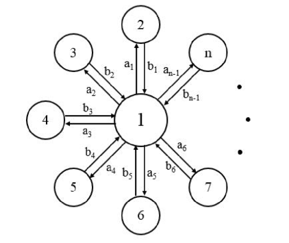
Figure 1: The star migration graph.

Then the connectivity matrix $L$ is an $n\times n$ $(n\geq 2)$ matrix:

$$L=\begin{pmatrix}-\displaystyle\sum_{i=1}^{n-1}a_{i}&b_{1}&b_{2}&b_{3}&\cdots&b_{n-1}\\ a_{1}&-b_{1}&0&0&\cdots&0\\ a_{2}&0&-b_{2}&0&\cdots&0\\ a_{3}&0&0&-b_{3}&\cdots&0\\ \vdots&\vdots&\vdots&\vdots&\ddots&\vdots\\ a_{n-1}&0&0&0&\cdots&-b_{n-1}\end{pmatrix}.$$ (4.1)

Denote $r_{i}={a_{i}}/{b_{i}}$ for $i=1,\dots,n-1$. A direct computation gives

$$\bm{\alpha}=\left(\displaystyle\frac{1}{1+s},\displaystyle\frac{r_{1}}{1+s},\dots,\displaystyle\frac{r_{n-1}}{1+s}\right),$$

where $s=\displaystyle\sum_{i=1}^{n-1}r_{i}$. Here we assume:

1. $H^{+}=\{1,2\}$ and $H^{-}=\{3,\dots,n\}$.

This assumption means that patch-$1$ and patch-$2$ are of high-risk, and all others are of low-risk.

For this example, we can compute

$$\check{I}_{j}^{(0)}=\begin{cases}\alpha_{j},&j=1,2,\\ \displaystyle\frac{d_{I}a_{j-1}\alpha_{1}}{d_{I}b_{j-1}+\gamma_{j}-\beta_{j}},&j=3,\dots,n,\end{cases}$$

and

$$\begin{split}h_{1}(d_{I})=&d_{I}\left[\left(-\sum_{k=1}^{n-1}a_{k}\right)\alpha_{1}+b_{1}\alpha_{2}+\sum_{k=3}^{n}\displaystyle\frac{d_{I}\alpha_{1}a_{k-1}b_{k-1}}{d_{I}b_{k-1}+\gamma_{k}-\beta_{k}}\right]+\alpha_{1}(\beta_{1}-\gamma_{1}).\\ h_{2}(d_{I})=&\alpha_{2}(\beta_{2}-\gamma_{2})>0\end{split}$$

It follows from Proposition 3.10 that $h_{1}(d_{I})$ is strictly decreasing and satisfies

$$\lim_{d_{I}\to 0}h_{1}(d_{I})=\alpha_{1}(\beta_{1}-\gamma_{1})>0,\;\;\text{and}\;\;\lim_{d_{I}\to\infty}h_{1}(d_{I})=\alpha_{1}(\beta_{1}-\gamma_{1})+\displaystyle\sum_{k=3}^{n}\alpha_{k}(\beta_{k}-\gamma_{k}).$$ (4.2)

By Lemma 2.5, we have that

$$\begin{split}&\lim_{d_{I}\to 0}s\left(d_{I}L+diag(\beta_{j}-\gamma_{j})\right)=\displaystyle\max_{1\leq k=\leq n}(\beta_{k}-\gamma_{k})>0,\\ &\lim_{d_{I}\to 0}s\left(d_{I}L+diag(\beta_{j}-\gamma_{j})\right)=\displaystyle\sum_{k=1}^{n}\alpha_{k}(\beta_{k}-\gamma_{k}).\end{split}$$

Since $s\left(d_{I}L+diag(\beta_{j}-\gamma_{j})\right)$ has the same sign as $R_{0}-1$ and is strictly decreasing for $d_{I}$, we have the following result.

Proposition 4.1.

Suppose $a_{k},b_{k}>0$ for $k=1,\dots,n-1$ and $(A)$ holds. Then the following statements hold:

1. If $\displaystyle\sum_{k=1}^{n}\alpha_{k}(\beta_{k}-\gamma_{k})>0$, then $R_{0}>1$ for any $d_{I}>0$. Moreover,

   1. if $\alpha_{1}(\beta_{1}-\gamma_{1})+\displaystyle\sum_{k=3}^{n}\alpha_{k}(\beta_{k}-\gamma_{k})\geq 0$, then $J^{+}=H^{+}$ and $J^{-}=H^{-}$ for any $d_{I}>0$;

   2. if $\alpha_{1}(\beta_{1}-\gamma_{1})+\displaystyle\sum_{k=3}^{n}\alpha_{k}(\beta_{k}-\gamma_{k})<0$, then there exists a unique $d_{I}^{**}$ such that $h_{1}(\tilde{d}_{I})=0$, and $J^{+}=H^{+}$ and $J^{-}=H^{-}$ for $0<d_{I}<d_{I}^{**}$, and $J^{+}=\{1\}$ and $J^{-}=\{2,\dots,n\}$, or $J^{+}=\{2\}$ and $J^{-}=\{1,3,\dots,n\}$ for $d_{I}>d_{I}^{**}$.

2. If $\displaystyle\sum_{k=1}^{n}\alpha_{k}(\beta_{k}-\gamma_{k})<0$, then $\alpha_{1}(\beta_{1}-\gamma_{1})+\displaystyle\sum_{k=3}^{n}\alpha_{k}(\beta_{k}-\gamma_{k})<0$, and there exists $d_{I}^{*}>0$ such that $R_{0}>1$ for $d_{I}<d_{I}^{*}$ and $R_{0}<1$ for $d_{I}>d_{I}^{*}$. Moreover,

   1. if $d_{I}^{**}\geq d_{I}^{*}$, where $d_{I}^{**}$ is defined as in $(i_{2})$, then $J^{+}=H^{+}$ and $J^{-}=H^{-}$ for $d_{I}<d_{I}^{*}$;

   2. if $d_{I}^{**}<d_{I}^{*}$, then $J^{+}=H^{+}$ and $J^{-}=H^{-}$ for $d_{I}<d_{I}^{**}$; and $J^{+}=\{1\}$ and $J^{-}=\{2,\dots,n\}$, or $J^{+}=\{2\}$ and $J^{-}=\{1,3,\dots,n\}$ for $d_{I}\in(d_{I}^{**},d_{I}^{*})$.

Remark 4.2.

From Proposition 4.1, we see that case $(i_{1})$ could hold when $\beta_{1}-\gamma_{1}$ is sufficiently large; case $(i_{2})$ could hold when $\beta_{1}-\gamma_{1}$ is sufficiently small but $\beta_{2}-\gamma_{2}$ is sufficiently large; and if both $\beta_{1}-\gamma_{1}$ and $\beta_{2}-\gamma_{2}$ are sufficiently small, case $(ii_{1})$ or $(ii_{2})$ could occur.

The asymptotic profile of the endemic equilibrium as $d_{I}\rightarrow 0$ can also be obtained from Theorem 3.16. To further illustrate our results, we give a numerical example of star graph with $n=4$. Let

$$L=\begin{pmatrix}-6&1&1&1\\ 1&-1&0&0\\ 2&0&-1&0\\ 3&0&0&-1\end{pmatrix}.$$

Then $\bm{\alpha}=(1/7,1/7,2/7,3/7)$. We choose $\beta_{1}=3,\beta_{2}=4,\beta_{3}=1,\beta_{4}=1$,$\gamma_{1}=1,\gamma_{2}=1,\gamma_{3}=2,\gamma_{4}=7$ such that $H^{+}=\{1,2\}$ and $H^{-}=\{3,4\}$, and $N=100$. Theorem 2.6 states that $R_{0}$ is strictly deceasing in $d_{I}$ with

$$\lim_{d_{I}\to 0}R_{0}=\max\left\{\frac{\beta_{j}}{\gamma_{j}}:j\in\Omega\right\}=4\ \ \ \text{and}\ \ \ \lim_{d_{I}\to\infty}R_{0}=\frac{\sum_{j\in\Omega}\alpha_{j}\beta_{j}}{\sum_{j\in\Omega}\alpha_{j}\gamma_{j}}=\frac{4}{5}.$$

In Figure 3, we plot $R_{0}$ as a function of $d_{I}$, which confirms Theorem 2.6. Here, $R_{0}-1$ changes sign at $d_{I}^{*}\approx 8.478$.

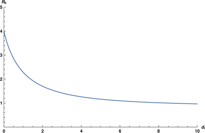
Figure 2: The basic reproduction number $R_{0}$ as a function of $d_{I}$.

Then we compute $h_{j}(d_{I})$, $j=1,2$. By Proposition 3.10, $h_{j}(d_{I})$ is constant or strictly decreasing in $d_{I}$. By (4.2), we expect

$$\lim_{d_{I}\rightarrow 0}h_{1}(d_{I})=\frac{2}{7}\ \ \ \text{and}\ \ \ \lim_{d_{I}\rightarrow\infty}h_{1}(d_{I})=-\frac{6}{7},$$

and $h_{2}(d_{I})=3/7$ for all $d_{I}>0$. These results are confirmed by Figure 3. Moreover, we have $h_{1}(0.549)\approx 0$. By $\sum_{j\in\Omega}\alpha_{j}(\beta_{j}-\gamma_{j})=-3/7<0$ and Proposition 4.1(ii), we expect that the profile of the endemic equilibrium changes at $d_{I}^{**}\approx 0.549$.

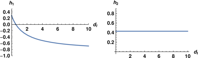
Figure 3: The graph of $h(d_{I})$.

In Figure 4, we plot the $S$ component of the endemic equilibrium as $d_{S}\rightarrow 0$, where $S_{j}^{*}=\displaystyle\lim_{d_{S}\rightarrow 0}S_{j}$ for $j=\{1,2,3,4\}$. From the figure, we see that $J^{+}=\{1,2\}$ and $J^{-}=\{3,4\}$ for $d_{I}\in(0,d_{I}^{**})$ and $J^{+}=\{2\}$ and $J^{-}=\{1,3,4\}$ for $d_{I}\in(d_{I}^{**},d_{I}^{*})$.

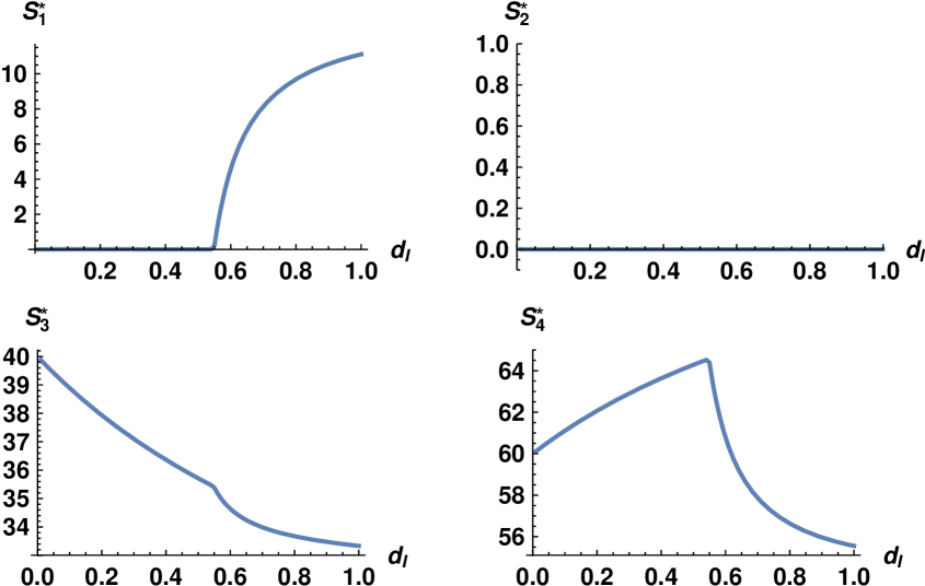
Figure 4: The $S$ component of the endemic equilibrium as $d_{S}\rightarrow 0$.

References

- [1] L. J. S. Allen, B. M. Bolker, Y. Lou, and A. L. Nevai. Asymptotic profiles of the steady states for an epidemic patch model. SIAM J. Appl. Math., 67(5):1283–1309, 2007.
- [2] L. J. S. Allen, B. M. Bolker, Y. Lou, and A. L. Nevai. Asymptotic profiles of the steady states for an SIS epidemic reaction-diffusion model. Discrete Contin. Dyn. Syst., 21(1):1–20, 2008.
- [3] R. M. Almarashi and C. C. McCluskey. The effect of immigration of infectives on disease-free equilibria. J. Math. Biol., 79(3):1015–1028, 2019.
- [4] L. Altenberg. Resolvent positive linear operators exhibit the reduction phenomenon. Proc. Natl. Acad. Sci. USA, 109(10):3705–3710, 2012.
- [5] R. M. Anderson and R. M. May. Infectious diseases of humans: dynamics and control. Oxford University Press, 1991.
- [6] J. Arino and P. van den Driessche. A multi-city epidemic model. Math. Popul. Stud., 10(3):175–193, 2003.
- [7] A. Berman and R. J. Plemmons. Nonnegative matrices in the mathematical sciences, volume 9 of Classics in Applied Mathematics. Society for Industrial and Applied Mathematics (SIAM), Philadelphia, PA, 1994.
- [8] F. Brauer, P. van den Driessche, and J.-H. Wu, editors. Mathematical epidemiology, volume 1945 of Lecture Notes in Mathematics. Springer-Verlag, Berlin, 2008. Mathematical Biosciences Subseries.
- [9] S.-S. Chen, J.-P. Shi, Z.-S. Shuai, and Y.-X. Wu. Spectral monotonicity of perturbed quasi-positive matrices with applications in population dynamics. Submitted.
- [10] R.-H. Cui, K.-Y. Lam, and Y. Lou. Dynamics and asymptotic profiles of steady states of an epidemic model in advective environments. J. Differential Equations, 263(4):2343–2373, 2017.
- [11] R.-H. Cui and Y. Lou. A spatial SIS model in advective heterogeneous environments. J. Differential Equations, 261(6):3305–3343, 2016.
- [12] K. Deng and Y. Wu. Dynamics of a susceptible-infected-susceptible epidemic reaction-diffusion model. Proc. Roy. Soc. Edinburgh Sect. A, 146(5):929–946, 2016.
- [13] O. Diekmann and J. A. P. Heesterbeek. Mathematical epidemiology of infectious diseases. Model building, analysis and interpretation. Wiley Series in Mathematical and Computational Biology. John Wiley & Sons, Ltd., Chichester, 2000.
- [14] M. C. Eisenberg, Z.-S. Shuai, J. H. Tien, and P. van den Driessche. A cholera model in a patchy environment with water and human movement. Math. Biosci., 246(1):105–112, 2013.
- [15] W.-E. Fitzgibbon and M. Langlais. Simple models for the transmission of microparasites between host populations living on noncoincident spatial domains. In Structured population models in biology and epidemiology, volume 1936 of Lecture Notes in Math., pages 115–164. Springer, Berlin, 2008.
- [16] D.-Z. Gao. Travel frequency and infectious diseases. SIAM J. Appl. Math., 79(4):1581–1606, 2019.
- [17] D.-Z. Gao and C.-P. Dong. Fast diffusion inhibits disease outbreaks. arXiv:1907.12229, 2019.
- [18] D.-Z. Gao and S.-G. Ruan. An SIS patch model with variable transmission coefficients. Math. Biosci., 232(2):110–115, 2011.
- [19] D.-Z. Gao, P. van den Driessche, and C. Cosner. Habitat fragmentation promotes malaria persistence. to appear in J. Math. Biol., 2019.
- [20] D.-H. Jiang, Z.-C. Wang, and L. Zhang. A reaction-diffusion-advection SIS epidemic model in a spatially-temporally heterogeneous environment. Discrete Contin. Dyn. Syst. Ser. B, 23(10):4557–4578, 2018.
- [21] Y. Jin and W.-D. Wang. The effect of population dispersal on the spread of a disease. J. Math. Anal. Appl., 308(1):343–364, 2005.
- [22] S. Karlin. Classifications of selection-migration structures and conditions for a protected polymorphism. In Evolutionary Biology, volume 14, pages 61–204. Plenum Press, New York, 1982.
- [23] K. Kuto, H. Matsuzawa, and R. Peng. Concentration profile of endemic equilibrium of a reaction-diffusion-advection SIS epidemic model. Calc. Var. Partial Differential Equations, 56(4):112, 2017.
- [24] H.-C. Li and R. Peng. Dynamics and asymptotic profiles of endemic equilibrium for SIS epidemic patch models. J. Math. Biol., 79(4):1279–1317, 2019.
- [25] H.-C. Li, R. Peng, and Z.-A. Wang. On a diffusive susceptible-infected-susceptible epidemic model with mass action mechanism and birth-death effect: analysis, simulations, and comparison with other mechanisms. SIAM J. Appl. Math., 78(4):2129–2153, 2018.
- [26] M. Y. Li and Z.-S. Shuai. Global stability of an epidemic model in a patchy environment. Can. Appl. Math. Q., 17(1):175–187, 2009.
- [27] M. Y. Li and Z.-S. Shuai. Global-stability problem for coupled systems of differential equations on networks. J. Differential Equations, 248(1):1–20, 2010.
- [28] A. L. Lloyd and R. M. May. Spatial heterogeneity in epidemic models. J. Theoret. Biol., 179(1):1–11, 1996.
- [29] P. Magal, G. F. Webb, and Y.-X. Wu. On a vector-host epidemic model with spatial structure. Nonlinearity, 31(12):5589–5614, 2018.
- [30] R. Peng. Asymptotic profiles of the positive steady state for an SIS epidemic reaction-diffusion model. I. J. Differential Equations, 247(4):1096–1119, 2009.
- [31] R. Peng and S.-Q. Liu. Global stability of the steady states of an SIS epidemic reaction-diffusion model. Nonlinear Anal., 71(1-2):239–247, 2009.
- [32] R. Peng and F.-Q. Yi. Asymptotic profile of the positive steady state for an SIS epidemic reaction-diffusion model: effects of epidemic risk and population movement. Phys. D, 259:8–25, 2013.
- [33] M. Salmani and P. van den Driessche. A model for disease transmission in a patchy environment. Discrete Contin. Dyn. Syst. Ser. B, 6(1):185–202, 2006.
- [34] H. L. Smith and P. Waltman. The theory of the chemostat. Dynamics of microbial competition, volume 13 of Cambridge Studies in Mathematical Biology. Cambridge University Press, Cambridge, 1995.
- [35] J. H. Tien, Z.-S. Shuai, M. C. Eisenberg, and P. van den Driessche. Disease invasion on community networks with environmental pathogen movement. J. Math. Biol., 70(5):1065–1092, 2015.
- [36] N. Tuncer and M. Martcheva. Analytical and numerical approaches to coexistence of strains in a two-strain SIS model with diffusion. J. Biol. Dyn., 6(2):406–439, 2012.
- [37] P. van den Driessche and J. Watmough. Reproduction numbers and sub-threshold endemic equilibria for compartmental models of disease transmission. Math. Biosci., 180:29–48, 2002.
- [38] W.-D. Wang and X.-Q. Zhao. An epidemic model in a patchy environment. Math. Biosci., 190(1):97–112, 2004.
- [39] W.-D. Wang and X.-Q. Zhao. An age-structured epidemic model in a patchy environment. SIAM J. Appl. Math., 65(5):1597–1614, 2005.
- [40] W.-D. Wang and X.-Q. Zhao. Basic reproduction numbers for reaction-diffusion epidemic models. SIAM J. Appl. Dyn. Syst., 11(4):1652–1673, 2012.
- [41] Y.-X. Wu, N. Tuncer, and M. Martcheva. Coexistence and competitive exclusion in an SIS model with standard incidence and diffusion. Discrete Contin. Dyn. Syst. Ser. B, 22(3):1167–1187, 2017.
- [42] Y.-X. Wu and X.-F. Zou. Asymptotic profiles of steady states for a diffusive SIS epidemic model with mass action infection mechanism. J. Differential Equations, 261(8):4424–4447, 2016.
- [43] X.-Q. Zhao. Dynamical systems in population biology. CMS Books in Mathematics/Ouvrages de Mathématiques de la SMC. Springer, Cham, second edition, 2017.
- [44] X.-Q. Zhao and Z.-J. Jing. Global asymptotic behavior in some cooperative systems of functional-differential equations. Canad. Appl. Math. Quart., 4(4):421–444, 1996.