Resilient Load Restoration in Microgrids Considering Mobile Energy Storage Fleets: A Deep Reinforcement Learning Approach

Abstract

Mobile energy storage systems (MESSs) provide mobility and flexibility to enhance distribution system resilience. The paper proposes a Markov decision process (MDP) formulation for an integrated service restoration strategy that coordinates the scheduling of MESSs and resource dispatching of microgrids. The uncertainties in load consumption are taken into account. The deep reinforcement learning (DRL) algorithm is utilized to solve the MDP for optimal scheduling. Specifically, the twin delayed deep deterministic policy gradient (TD3) is applied to train the deep Q-network and policy network, then the well trained policy can be deployed in on-line manner to perform multiple actions simultaneously. The proposed model is demonstrated on an integrated test system with three microgrids connected by Sioux Falls transportation network. The simulation results indicate that mobile and stationary energy resources can be well coordinated to improve system resilience.

I Introduction

Recent major blackouts caused by extreme events lead to catastrophic consequences for the economy and society [1]. Load restoration is of paramount importance in resilient smart grids [2]. Great progress has been made in coordinating multiple energy resources to effectively restore electricity supply to critical loads after major blackouts [3]. Microgrids are well utilized to consolidate stationary energy resources [4]. Moreover, with the increasing installation of charging/discharging facilities [5], microgrids can provide plug-and-play integration of mobile energy storage systems (MESSs) for effective service restoration. The importance of integrating mobile energy resources into critical load restoration in smart grid has been increasingly recognized in recent studies [6, 7, 8]. EPRI and Department of Defense of the U.S. initiated a project to demonstrate a containerized grid support storage system featuring utility capacity up to 2 MWh committed to enhancing energy security at military facilities [9]. Reference [10] proposes a microgrid-based critical load restoration by adaptively forming microgrids and positioning mobile emergency resources after power disruptions. Reference [11] implements resilient routing and scheduling of mobile power sources via a two-stage framework. However, the optimal scheduling is generally formulated as mixed-integer convex program, which is NP-hard and computationally expensive, in terms of a large number of integer or binary variables in large-scale systems [12]. In addition, accurate forecast information is necessary in the optimization model [13].

Recent advances in deep reinforcement learning (DRL) give rise to tremendous success in solving challenging decision-making problem [14, 15]. In general, the decision-making problem under uncertainties is formulated using Markov decision process (MDP) [16] and solved iteratively by data-driven DRL algorithms [15]. The application of deep reinforcement learning in energy management systems has been increasingly recognized. Reference [17] presents a reinforcement learning approach for optimal distributed energy management in a microgrid. A DRL-based economic dispatch in microgrid is proposed in [18]. Reference [19] developed an MDP formulation for the joint bidding and pricing problem and applied DRL algorithm to solve it. Reference [12] proposes a demand response for home energy management based on DRL. An MDP formulation for electrical vehicle charging is proposed to jointly coordinate a set of charging stations [20]. A dynamic distribution network reconfiguration using reinforcement learning is proposed in [21]. However, research in this area is still in the early stage, the benefit of applying DRL in coordinated scheduling of stationary and mobile energy resources has not yet been fully investigated and further studies are needed.

To address the aforementioned issue, a novel MDP formulation for critical load restoration in microgrids is proposed considering the stationary and mobile energy resources. Uncertainties in load consumption are taken into account. The agent aims to maximize the service restoration in microgrids by jointly coordinating the resource dispatching of microgrids and scheduling of MESS. The MESS fleets are dynamically dispatched among microgrids for load restoration in coordination with microgrid operation. The proposed model is solved by twin delayed deep deterministic policy gradient (TD3) [22], which is an actor-critic algorithm that can deal with discrete or continuous variables in state and action space.

The remainder of this paper is organized as follows. Section II mathematically describes the scheduling of MESSs and integrated service restoration strategy. Section III develops the MDP formulation and deep reinforcement learning algorithm. Section IV provides case studies and the paper is concluded in Section V.

II Mathematical modeling

II-A Uncertainties Modeling

Uncertainties have been considered including forecasting errors in load consumption. A normal distribution is used to represent the forecasting error of load consumption [8]. At each time step $t$, the load will be simulated as exogenous information input.

II-B Scheduling of Mobile Energy Storage Fleets

A transportation network is modeled as a weighted graph $\mathcal{G}_{\text{T}}=(\mathcal{N}_{\text{T}},\mathcal{E}_{\text{T}},\mathcal{W}_{\text{T}})$, where $\mathcal{N}_{\text{T}}$ is the nodes set, while $\mathcal{E}_{\text{T}}$ denotes the edges set of roads with the edge distance $w\in\mathcal{W}_{\text{T}}$. A set of microgrids $\mathcal{M}$ indexed by $m$ and a set of depots $\mathcal{D}$ are located in the transportation network $\mathcal{G}_{\text{T}}$. Location mappings $f_{\text{M}}:\mathcal{M}\rightarrow\mathcal{N}_{\text{T}}$ and $f_{\text{D}}:\mathcal{D}\rightarrow\mathcal{N}_{\text{T}}$ denote microgrids and depots’ locations in the transportation network, respectively. $\Omega$ represents an MESS fleet. An MESS $\omega\in\Omega$ is initially located at a depot $d\in\mathcal{D}$, where it starts and travels among microgrids to provide power supply to power grids, finally it goes back to a depot.

The scheduling of MESS fleets is defined as a sequence of trips. An MESS $\omega$’s current location at $t$ is represented by $n_{\omega}^{t}$, which is generally defined as the node in the transportation network [23]. In addition, MESS may change destination during its’ movement without having to arrive at the next destination, that is, MESS may be on the edge at $t$, so the location of MESS is defined as $n_{\omega}^{t}\in\mathcal{N}_{\text{T}}\cup\{(\hat{n},\delta_{\hat{n}},\check{n},\delta_{\check{n}})|(\hat{n},\check{n})\in E_{\text{T}},\delta_{\hat{n}}+\delta_{\check{n}}=w_{\hat{n}\check{n}},\delta_{\hat{n}}\geq 0,\delta_{\check{n}}\geq 0\}$, where the $\{(\hat{n},\delta_{\hat{n}},\check{n},\delta_{\check{n}})|(\hat{n},\check{n})\in E_{\text{T}},\delta_{\hat{n}}+\delta_{\check{n}}=w_{\hat{n}\check{n}},\delta_{\hat{n}}\geq 0,\delta_{\check{n}}\geq 0\}$ denotes a location on the edge $(\hat{n},\check{n})\in E_{\textit{T}}$, $\delta_{\hat{n}}$ and $\delta_{\check{n}}$ depict the location’s distance to corresponding nodes, and $w_{\hat{n}\check{n}}$ represents the edge length.

The movement decision for MESS $\omega$ at $t$ is to designate the destination $\kappa_{\omega}^{t}\in\mathcal{M}\cup\mathcal{D}$, which specifies the destination to one of microgrids or stations. The MESS $\omega$ moves from the current location $n_{\omega}^{t}$ and follows the movement decision $\kappa_{\omega}^{t}$ to the designated destination. And It is assumed that the MESS $\omega$ always takes the shortest path, which is determined by the Dijkstra’s algorithm [24]. Therefore, a location function $f_{\text{L}}$ is defined to obtain the next location $n_{\omega}^{t+1}$ in graph $G_{\text{T}}$, by using Dijkstra algorithm based on current location $n_{\omega}^{t}$ and designated destination $\kappa_{\omega}^{t}$. Thus, we have

$$n_{\omega}^{t+1}=f_{\text{L}}(n_{\omega}^{t},\kappa_{\omega}^{t}),\forall\omega,t$$ (1)

Binary variables $\zeta_{\omega m}^{t}$ denote if MESS $\omega$ stays at microgrid $m$ during the interval $t$, which is described as follows.

$$\zeta_{\omega m}^{t}=\begin{cases}1,&\text{If}~{}n_{\omega}^{t}=n_{\omega}^{t+1}~{}\text{and}~{}n_{\omega}^{t}\in f_{\text{M}}(m)\\ 0,&\text{Otherwise}\\ \end{cases},\forall\omega,m,t$$ (2)

MESS fleets can exchange power with microgrids by charging from or discharging to microgrids. The operation constraints are described as follows.

$$\sum_{m\in M}\zeta_{\omega m}^{t}\leq 1,\forall\omega,t$$ (3)

$$-\overline{P}^{\omega}_{\text{ch}}\sum_{m\in M}\xi^{t}_{\omega m}\leq P_{\omega}^{t}\leq\overline{P}^{\omega}_{\text{dch}}\sum_{m\in M}\xi^{t}_{\omega m},\forall\omega,t$$ (4)

$$\begin{aligned} \text{SOC}_{\omega}^{t+1}=\begin{cases}\text{SOC}_{\omega}^{t}-\frac{\eta_{\mathrm{ch}}^{\omega}P_{\omega}^{t}}{E_{\text{c}}^{\omega}}\Delta_{t},&\text{if}~{}P_{\omega}^{t}<0\\ \text{SOC}_{\omega}^{t}-\frac{P_{\omega}^{t}}{\eta_{\text{dch}}^{\omega}E_{\text{c}}^{\omega}}\Delta_{t},&\text{if}~{}P_{\omega}^{t}\geq 0\\ \end{cases},\forall\omega,t\end{aligned}$$ (5)

$$\uline{\text{SOC}}_{\omega}\leq\text{SOC}_{\omega}^{t}\leq\overline{\text{SOC}}_{\omega},\forall\omega,t$$ (6)

where $P_{\omega}^{t}$ represent the charging/discharging power of MESS $\omega$ from/to microgrid $m$ at interval $t$, negative power depicts that MESS charges from microgrids while positive power means that MESS discharge to microgrid. $\overline{P}^{\omega}_{\text{ch}}$ and $\overline{P}^{\omega}_{\text{dch}}$ are maximum charging/discharging power of MESS $\omega$. $\text{SOC}_{\omega}^{t}$ indicates the state-of-charge (SOC) of MESS $\omega$ at time point $t$. $\uline{\text{SOC}}_{\omega}$ and $\overline{\text{SOC}}_{\omega}$ provide the prescribed minimum and maximum level of SOC. $\eta_{\text{ch}}^{\omega}$ and $\eta_{\text{dch}}^{\omega}$ are charging/discharging efficiency. $E^{\omega}_{c}$ indicates the battery capacity of MESS $\omega$. Constraints (3) indicates that an MESS can only stay at no more than one microgrid, which is also implicated in the Equation (2). Constraint (4) shows the relation between charging/discharging and temporal-spatial behaviors. That is, only when staying at a microgrid $m$ can MESS $\omega$ charge or discharge to exchange power. Equation (5) calculates the SOC of MESS $\omega$ and Constraint (6) sets the upper and lower bound for SOC.

II-C Joint Service Restoration

The operation constraints of microgrids are as follows.

$$P_{\text{dg},m}^{t}+\sum_{\omega\in\Omega}\xi_{\omega m}^{t}P_{\omega}^{t}=P_{\text{r},m}^{t},\forall m,t$$ (7)

$$Q_{\text{dg},m}^{t}=Q_{\text{r},m}^{t},\forall m,t$$ (8)

$$0\leq P_{\text{r},m}^{t}\leq P_{\text{load},m}^{t},\forall m,t$$ (9)

$$Q_{\text{r},m}^{t}=P_{\text{r},m}^{t}\tan(\cos^{-1}\varphi_{m}),\forall m,t$$ (10)

$$0\leq P_{\text{dg},m}^{t}\leq\overline{P}_{\text{dg},m},\forall m,t$$ (11)

$$-\overline{Q}_{\text{dg},m}\leq Q_{\text{dg},m}^{t}\leq\overline{Q}_{\text{dg},m},\forall m,t$$ (12)

$$E_{\text{dg},m}^{t+1}=E_{\text{dg},m}^{t}-P_{\text{dg},m}^{t+1}\Delta t,\forall m,t$$ (13)

$$\uline{E}_{\text{dg},m}^{\text{min}}\leq E_{\text{dg},m}^{t}\leq\overline{E}_{\text{dg},m}\forall m,t$$ (14)

where $P_{\text{dg},m}^{t},Q_{\text{dg},m}^{t}$ are the active/reactive power generation of equivalent dispatchable DG in microgrid $m$ in interval $t$, respectively. $\overline{P}_{\text{dg},m},\overline{Q}_{\text{dg},m}$ are the maximum active/reactive power generation, respectively. $P_{\text{r},m}^{t},Q_{\text{r},m}^{t}$ are active/reactive load restoration in microgrid $m$, respectively. $\varphi_{m}$ is the power factor. $E_{\text{dg},m}^{t}$ is the energy of equivalent DG. $\overline{E}_{\text{dg},m}^{t}$ and $\uline{E}_{\text{dg},m}^{t}$ are the energy capacity and minimum energy reserve in microgrid $m$. Constraints (7)-(8) describe the active/reactive power balance at microgrid $m$ in interval $t$. It takes into account the power generation of dispatachable DG and mobile energy storage by considering if the location of MESSs. Equations (9)-(10) constrain the load restoration and power factor. Constraints (11)-(12) depict the power generation capacity. Equation (13) calculates the energy in each microgrid. Constraint (14) presents the upper and lower bounds of energy.

In the wake of major disturbances, the restoration strategy is implemented across multiple microgrids over the horizon to reach a higher level of resilience, which is more focused on the system cost in this work. Therefore, the objective is formulated as follows to minimize the system overall cost.

$$\min~{}\sum_{t\in T}\bigg{[}\sum_{m\in\mathcal{M}}W_{m}(P_{\text{load},m}^{t}-P_{\text{r},m}^{t})+\sum_{m\in\mathcal{M}}C_{\text{gen},m}P_{\text{dg},m}^{t}$$

$$+\sum_{\omega\in\Omega}C_{\text{bat},\omega}|P_{\omega}^{t}|+\sum_{\omega\in\Omega}C_{\text{tran},\omega}(1-\sum_{m\in\mathcal{M}}\zeta_{\omega m}^{t})\bigg{]}\Delta T$$ (15)

where the overall cost is composed of four parts. The first term $\sum_{t\in T}\sum_{m\in\mathcal{M}}W_{m}(P_{\text{load},m}^{t}-P_{\text{r},m}^{t})$ represents the customer interruption cost. $\sum_{t\in T}\sum_{m\in\mathcal{M}}C_{\text{gen},m}P_{\text{dg},m}^{t}$ is the microgrids generation cost. The third term $\sum_{t\in T}\sum_{\omega\in\Omega}C_{\text{bat},\omega}|P_{\omega}^{t}|$ shows the MESS battery maintenance cost. The last term $\sum_{t\in T}\sum_{\omega\in\Omega}C_{\text{tran},\omega}V_{\text{avg},\omega}(1-\sum_{m\in\mathcal{M}}\zeta_{\omega m}^{t})$ calculates the transportation cost of MESSs.

III Deep Reinforcement Learning Algorithm

III-A Markov Decision Process

The sequential decision-making problem in a stochastic environment is formulated by Markov decision processes (MDPs). In an MDP, an agent observes the state $s_{t}$ at each time step $t\in\mathcal{T}$ and continually interacts with an environment by following a policy $\pi$ to select actions $a$. In response to the actions, the environment presents new states $s_{t+1}$ and give rise to rewards $r_{t}$ to the agent. An MDP is defined by a 4-tuple $(\mathcal{S},\mathcal{A},\mathcal{P},\mathcal{R})$, where $\mathcal{S},\mathcal{A},\mathcal{P},\mathcal{R}$ are the state space, action space, transition probability functions that satisfy Markov property [16] (i.e., the next state is only dependent on present state and action), and reward functions. The detailed formulation is described as follows.

The state is a vector defined as $s_{t}=\{t,P_{\text{load},m}^{t},n_{\omega}^{t},\text{SOC}_{\omega}^{t},E_{\text{dg},m}^{t}\}\in\mathcal{S}$, presenting information on time step, load, the location and SOC of MESSs, and energy in microgrids.

Furthermore, the action is a vector consisting of decision variables on the designated destination of MESSs charging/discharging behavior of MESSs and generation output in microgrids. The action is defined as $a_{t}=\{\kappa_{\omega}^{t},P_{\omega}^{t},P_{\text{dg},m}^{t}\}\in\mathcal{A}$. It is noted that $\kappa_{\omega}^{t}$ represents categorical action and needs to be one-hot encoded.

The state transition $\mathcal{P}:\mathcal{S}\times\mathcal{A}\times\mathcal{S}\rightarrow[0,1]$ represents the dynamics of the environment, the transition function indicates the mapping between states at two adjacent time points, so we have $s_{t+1}=\mathcal{P}(s_{t},a_{t})$. To model the uncertainties in load consumption. the exogenous information $P_{\text{load},m}^{t}$ in state vector $s_{t}$ are random variables. Based on the state and action, the next state $s_{t+1}$ can be obtained. In reinforcement learning, the $\mathcal{P}$ is unknown and needs to be learned through interactions between the agent and the environment [25].

The reward function is defined as $\mathcal{R}:\mathcal{S}\times\mathcal{A}\times\mathcal{S}\rightarrow\mathbb{R}$, where $r_{t}=\mathcal{R}(s_{t},a_{t},s_{t+1})$ is the immediate reward the agent receives by taking action $a_{t}$ given state $s_{t}$. The immediate reward $r_{t}$ has two components to take into objectives and penalty violating constraints [18]. The detailed definition is as follows.

$$r_{t}=\lambda_{1}R_{\text{obj},t}+\lambda_{2}C_{\text{pen},t}$$ (16)

where $\lambda_{1},\lambda_{2}$ are coefficients. $R_{\text{obj},t}=[\sum_{m\in\mathcal{M}}W_{m}P_{\text{r},m}^{t}-\sum_{m\in\mathcal{M}}C_{\text{gen},m}P_{\text{dg},m}^{t}-\sum_{\omega\in\Omega}C_{\text{bat},\omega}|P_{\omega}^{t}|-\sum_{\omega\in\Omega}C_{\text{tran},\omega}V_{\text{avg},\omega}(1-\sum_{m\in\mathcal{M}}\zeta_{\omega m}^{t})]\Delta T$ relates to objective function (II-C) and is obtained by ignoring the constant term and taking minus sign, thus the cost minimization is transformed into a reward maximization problem. The second term $C_{\text{pen},t}$ is Lagrangian penalty term incurred by violation of constraints.

III-B Twin Delayed Deep Deterministic Policy Gradient

In reinforcement learning, the return is defined as the sum of discounted reward $G_{t}=\sum_{i=t}^{T}\gamma^{(i-t)}r(s_{i},a_{i})$, where $\gamma\in[0,1]$ is the discount factor. A policy $\pi:\mathcal{S}\rightarrow\mathcal{A}$ is a mapping from states to selecting actions, i.e., stochastic policy $a_{t}\sim\pi(\cdot|s_{t})$ or deterministic policy $a_{t}=\pi(s_{t})$. Solving an MDP is to find a policy $\pi$ that maximizes the expected return $\operatorname{\mathbb{E}}_{a_{t},s_{t}}[G_{0}]$.

In order to deal with continuous and discrete variables in state and action space, an actor-critic algorithm is adopted [26], e.g. deep deterministic policy gradient (DDPG) and twin delayed deep deterministic policy gradient (TD3), which concurrently learn Q-functions and a policy. It uses off-policy data and the Bellman equation to learn the Q-function, and uses the Q-function to learn the policy $\pi_{\phi}$ parameterized with $\phi$[25].

In Q-learning of TD3, the Q-function is estimated by a differentiable function approximator $Q_{\theta}(s,a)$, which is a neural network with weights $\theta$ as a Q-network. The Q-network can be learned to reduce the mean-squared Bellman error. To make the training converge and stable, a separate target Q-network $Q_{\theta^{\prime}}$ and a target policy network $\pi_{\phi^{\prime}}$ are utilized to generate optimal target value [15]. Therefore a sequence of loss functions $L(\theta)$ is set up by the mean-squared Bellman error as $L(\theta)=\operatorname{\mathbb{E}}_{s_{t},a_{t},r_{t}}[(Q_{\theta}(s_{t},a_{t})-y_{t})^{2}]$, where the target value $y_{t}$ is defined as $y_{t}=r_{t}+\gamma\max_{a_{t+1}}Q_{\theta^{\prime}}(s_{t+1},\pi_{\phi^{\prime}}(s_{t+1}))$.

The Q-network is updated by one step gradient descent using $L(\theta)$. A soft target update is used for actor-critic algorithm [26], the target networks are updated by Polyak averaging, $\theta^{\prime}=\tau\theta+(1-\tau)\theta^{\prime},\phi^{\prime}=\tau\phi+(1-\tau)\phi^{\prime}$, where $\tau\in[0,1]$ is the Polyak hyperparameter (usually $\tau\ll 1$). Furthermore, TD3 concurrently learns two Q-networks, $Q_{\theta_{1}}$ and $Q_{\theta_{2}}$ by minimizing mean-squared Bellman error. By upper-bounding the less biased value approximator $Q_{\theta_{2}}$ with the biased estimate $Q_{\theta_{1}}$, a single target update for clipped Double Q-learning is obtained by taking the minimum between the two Q-networks:

$$y_{t}=r_{t}+\gamma\min_{i=1,2}Q_{\theta^{\prime}_{i}}(s_{t+1},\pi^{\prime}_{\phi^{\prime}}(s_{t+1}))$$ (17)

Then $Q_{\theta_{1}}$ and $Q_{\theta_{2}}$ are updated by minimizing the corresponding mean-squared Bellman error as follows.

$$L(\theta_{i})=\operatorname{\mathbb{E}}_{s_{t},a_{t},r_{t}}[(Q_{\theta_{i}}(s_{t},a_{t})-y_{t})^{2}],\forall i=1,2$$ (18)

Target smoothing regularization is to add a small amount of random noise $\tilde{\epsilon}$ to the target policy network in target update and averaging over mini-batches. The modified target actions $\tilde{a}$ and target values $y_{t}$ are as follows.

$$\tilde{a}_{t+1}=\pi_{\phi^{\prime}}(s_{t+1})+\tilde{\epsilon},~{}\tilde{\epsilon}\sim\text{clip}(\mathcal{N}(0,\tilde{\sigma}^{2}),-c,c)$$ (19)

$$y_{t}=r_{t}+\gamma\min_{i=1,2}Q_{\theta^{\prime}_{i}}(s_{t+1},\tilde{a}_{t+1})$$ (20)

where the added noise is a normal distribution with zero-mean and standard deviation $\tilde{\sigma}$, and clipped by a hyperparameter $c$.

The Policy learning of TD3 is to find a policy $\pi_{\phi}(s_{t})$ that maximizes the expected discounted return $J(\phi)=\operatorname{\mathbb{E}}_{s_{t},a_{t}}[G_{0}]\approx\operatorname{\mathbb{E}}_{s_{t}}[Q_{\theta}(s_{t},\pi_{\phi}(s_{t}))]$ [22]. The policy network is updated by applying the chain rule to the $J(\phi)$ with respect to the actor parameters $\phi$ and gradient ascent is implemented. The policy $\pi_{\phi}$ is optimized with respect to $Q_{\theta_{1}}$ to maximize the expected return $J(\phi)$, so the policy learning is written as:

$$\nabla_{\phi}J(\phi)=\operatorname{\mathbb{E}}_{s_{t}}[\nabla_{a}Q_{\theta_{1}}(s_{t},a_{t})|_{a_{t}=\pi_{\phi}(s_{t})}\nabla_{\phi}\pi_{\phi}(s_{t})]$$ (21)

In addition, the policy network $\pi_{\phi}$ is updated at a lower frequency than the value network $Q_{\theta_{1}}$, in order to reduce error before introducing a policy update [22].

IV Case Studies

The case studies are implemented on an integrated test system, based on Sioux Falls transportation network and three microgrids, to verify the effectiveness of the proposed service restoration strategy.

IV-A Test Systems

Figure 1: An integrated test system with a Sioux Falls transportation network connecting three microgrids.

Fig. 1 shows an integrated test system with microgrids connected by the Sioux Falls transportation network. The length of the entire time horizon $T_{\text{H}}$ is set to 24-h and the length of interval is 1-h. A depot is located at node #10 in the transportation network. There are three microgrids located at nodes #2, #12, #21 in the transportation network, respectively. The operational parameters of microgrids are shown in Table I. The predicted value of industrial, commercial and residential loads, as well as prediction intervals could be obtained in [8]. The parameters for MESS refers to [8]. The customer interruption cost for industrial, commercial and residential loads are $\$8/\text{kWh}$, $\$10/\text{kWh}$ and $\$2/\text{kWh}$, respectively. The unit generation cost in microgrid is $\$0.5/\text{kWh}$. The unit battery maintenance cost is $\$0.2/\text{kWh}$. The unit transportation cost is $\$80/\text{h}$.

TABLE I: Generation Resources and Local Loads for microgrids

Microgrid #		1	2	3
Generation	$\overline{P}_{\text{dg},m}$ (MW)	1.0	1.80	1.20
	$\overline{Q}_{\text{dg},m}$ (MVar)	0.8	1.5	1.0
	$\overline{E}_{\text{dg},m}$ (MWh)	20	35	23
	$\uline{E}_{\text{dg},m}$ (MWh)	2.0	3.5	2.3
Load	Peak load (MW)	3.0	3.0	3.0
	Power factor	0.9	0.9	0.9
	Load type	C	R	I

IV-B Simulation Results

The total cost is $\$351172$, with the customer interruption cost $\$309859$, microgrid generation cost $\$34872$, MESS generations cost $\$4600$ and transportation cost $\$1840$. The load restorations in three microgrids are $72.92\%,56.66\%$ and $50.76\%$, respectively.

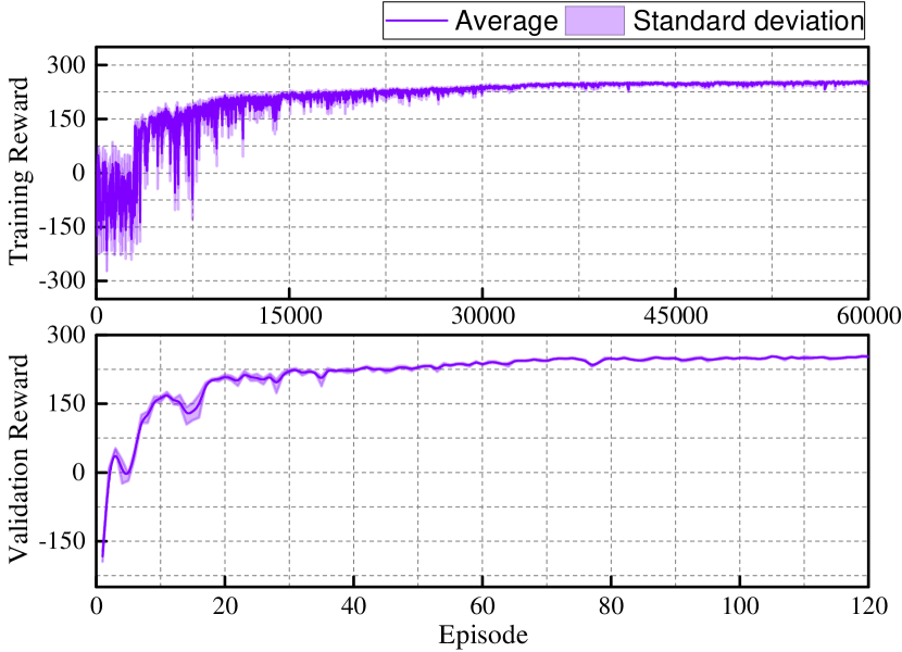
Figure 2: Learning and validation curves.

Fig. 2 illustrates the evolution of learning and validation rewards over 60000 episodes. A purely exploratory policy is carried out for the first 3000 episodes. Then, an off-policy exploration strategy is adopted with Gaussian noise. In the learning curve, the average and standard deviation are obtained every 10 episodes. In the validation curve, the validation is evaluated every 500 episodes over 20 episodes with no exploration noise. It can be seen that the learning process converges to a suboptimal policy in 40000 episodes. The results indicate that the proposed approach can learn a policy to maximize the cumulative rewards. After learning, the model can be deployed in on-line manner.

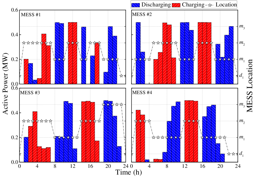
Figure 3: Scheduling results of the MESS fleets.

Fig. 3 presents the charging/discharging schedule with respect to the position of MESS. The bar shows the charging/discharging active power while the dash lines with asterisks and right Y-axis indicates the MESS’s movements. The dynamic scheduling of MESS optimizes the trip chain of MESSs and corresponding charging/discharging behaviors.

The simulation result shows that MESSs transport energy among microgrids to restore critical loads by charging from some microgrids and discharging to others. For example, it is observed that MESS #1 is dispatched between microgrid #1 and microgrid #2. The MESS #1 initially moves to microgrid #2 from depot and charges at microgrid #2. Next, it moves back and forth between microgrid #2 and microgrid #1 in (07:00-22:00) to transfer energy. The integration of MESSs and coordination with microgrids can leverage the MESSs mobility. Also, the MESSs can carry out load shifting within the same microgrid. For instance, MESS #3 charges at microgrid #2 in (01:00-02:00) and discharges in (02:00-07:00). The results highlight the importance of effective utilization of MESSs mobility and flexibility.

V Conclusions

This paper presents a novel MDP formulation for service restoration strategy in microgrids by coordinating the scheduling of MESSs and resource dispatching of microgrids. The DRL algorithms are leveraged to solve the formulated sequential decision-making problem with consideration of uncertainties in load consumption. The well trained policy can be deployed in on-line manner and is computationally efficient. The simulation results verify the effectiveness of MESSs mobility that transport energy among microgrids to facilitate load restoration. Mobile and stationary resources can be jointly coordinated to enhance system resilience.

References

- [1] Z. Bie, Y. Lin, G. Li, and F. Li, “Battling the Extreme: A Study on the Power System Resilience,” Proc. IEEE, vol. 105, no. 7, pp. 1253–1266, 2017.
- [2] Y. Wang, C. Chen, J. Wang, and R. Baldick, “Research on Resilience of Power Systems Under Natural Disasters—A Review,” IEEE Trans. Power Syst., vol. 31, no. 2, pp. 1604–1613, 2016.
- [3] Y. Xu, C. C. Liu, K. P. Schneider, F. K. Tuffner, and D. T. Ton, “Microgrids for service restoration to critical load in a resilient distribution system,” IEEE Trans. Smart Grid, vol. 9, no. 1, pp. 426–437, 2018.
- [4] C. Chen, J. Wang, and D. Ton, “Modernizing Distribution System Restoration to Achieve Grid Resiliency Against Extreme Weather Events: An Integrated Solution,” Proc. IEEE, vol. 105, no. 7, pp. 1267–1288, 2017.
- [5] S. Yao, P. Wang, and T. Zhao, “Transportable Energy Storage for More Resilient Distribution Systems with Multiple Microgrids,” IEEE Trans. Smart Grid, vol. 10, no. 3, pp. 3331–3341, 2019.
- [6] S. Yao, T. Zhao, H. Zhang, P. Wang, and L. Goel, “Two-stage stochastic scheduling of transportable energy storage systems for resilient distribution systems,” in 2018 IEEE Int. Conf. Probabilistic Methods Appl. to Power Syst., 2018, pp. 1–6.
- [7] J. Kim and Y. Dvorkin, “Enhancing Distribution System Resilience With Mobile Energy Storage and Microgrids,” IEEE Trans. Smart Grid, vol. 10, no. 5, pp. 4996–5006, sep 2019.
- [8] S. Yao, P. Wang, X. Liu, H. Zhang, and T. Zhao, “Rolling Optimization of Mobile Energy Storage Fleets for Resilient Service Restoration,” IEEE Trans. Smart Grid, vol. PP, no. 99, pp. 1–1, 2019.
- [9] Department of Defense, “Transportable Microgrid with Energy Storage,” Tech. Rep., 2016. [Online]. Available: https://serdp-estcp.org/Program-Areas/Energy-and-Water/Energy/Microgrids-and-Storage/EW-201605
- [10] L. Che and M. Shahidehpour, “Adaptive Formation of Microgrids With Mobile Emergency Resources for Critical Service Restoration in Extreme Conditions,” IEEE Trans. Power Syst., vol. 34, no. 1, pp. 742–753, 2019.
- [11] S. Lei, C. Chen, H. Zhou, and Y. Hou, “Routing and Scheduling of Mobile Power Sources for Distribution System Resilience Enhancement,” IEEE Trans. Smart Grid, vol. PP, no. 99, pp. 1–1, 2018.
- [12] R. Lu, S. H. Hong, and M. Yu, “Demand Response for Home Energy Management using Reinforcement Learning and Artificial Neural Network,” IEEE Trans. Smart Grid, vol. PP, no. c, pp. 1–1, 2019.
- [13] E. Mocanu, D. C. Mocanu, P. H. Nguyen, A. Liotta, M. E. Webber, M. Gibescu, and J. G. Slootweg, “On-line Building Energy Optimization using Deep Reinforcement Learning,” IEEE Trans. Smart Grid, vol. 99, no. PP, pp. 1–1, 2018.
- [14] D. Silver, J. Schrittwieser, K. Simonyan, I. Antonoglou, A. Huang, A. Guez, T. Hubert, L. Baker, M. Lai, A. Bolton, Y. Chen, T. Lillicrap, F. Hui, L. Sifre, G. Van Den Driessche, T. Graepel, and D. Hassabis, “Mastering the game of Go without human knowledge,” Nature, vol. 550, no. 7676, pp. 354–359, 2017.
- [15] V. Mnih, K. Kavukcuoglu, D. Silver, A. A. Rusu, J. Veness, M. G. Bellemare, A. Graves, M. Riedmiller, A. K. Fidjeland, G. Ostrovski, S. Petersen, C. Beattie, A. Sadik, I. Antonoglou, H. King, D. Kumaran, D. Wierstra, S. Legg, and D. Hassabis, “Human-level control through deep reinforcement learning,” Nature, vol. 518, no. 7540, p. 529, 2015.
- [16] T. J. Sheskin, Markov Chains and Decision Processes for Engineers and Managers. CRC Press, 2011.
- [17] E. Foruzan, L. K. Soh, and S. Asgarpoor, “Reinforcement Learning Approach for Optimal Distributed Energy Management in a Microgrid,” IEEE Trans. Power Syst., vol. 33, no. 5, pp. 5749–5758, 2018.
- [18] W. Liu, P. Zhuang, H. Liang, J. Peng, and Z. Huang, “Distributed Economic Dispatch in Microgrids Based on Cooperative Reinforcement Learning,” IEEE Trans. Neural Networks Learn. Syst., vol. 29, no. 6, pp. 2192–2203, 2018.
- [19] H. Xu, H. Sun, D. Nikovski, S. Kitamura, K. Mori, and H. Hashimoto, “Deep Reinforcement Learning for Joint Bidding and Pricing of Load Serving Entity,” IEEE Trans. Smart Grid, vol. PP, no. 99, pp. 1–1, 2019.
- [20] N. Sadeghianpourhamami, J. Deleu, and C. Develder, “Definition and evaluation of model-free coordination of electrical vehicle charging with reinforcement learning,” IEEE Trans. Smart Grid, vol. PP, no. 99, pp. 1–1, 2018.
- [21] Y. Gao, J. Shi, W. Wang, and N. Yu, “Dynamic Distribution Network Reconfiguration Using Reinforcement Learning,” 2019 IEEE Int. Conf. Commun. Control. Comput. Technol. Smart Grids, pp. 1–7, 2019.
- [22] S. Fujimoto, H. van Hoof, and D. Meger, “Addressing Function Approximation Error in Actor-Critic Methods,” 35th Int. Conf. Mach. Learn., 2018.
- [23] X. Yu, S. Gao, X. Hu, and H. Park, “A Markov decision process approach to vacant taxi routing with e-hailing,” Transp. Res. Part B Methodol., vol. 121, pp. 114–134, 2019.
- [24] T. H. Cormen, Introduction to algorithms. MIT press, 2009.
- [25] R. S. Sutton and A. G. Barto, Reinforcement Learning: An Introduction. The MIT Press, 2018.
- [26] T. P. Lillicrap, J. J. Hunt, A. Pritzel, N. Heess, T. Erez, Y. Tassa, D. Silver, and D. Wierstra, “Continuous control with deep reinforcement learning,” in Int. Conf. Learn. Represent. (2016 ICLR), 2016.