A Rational Finance Explanation of the Stock Predictability Puzzle

Abstract      In this paper, we address one of the main puzzles in finance observed in the stock market by proponents of behavioral finance: the stock predictability puzzle. We offer a statistical model within the context of rational finance which can be used without relying on behavioral finance assumptions to model the predictability of stock returns. We incorporate the predictability of stock returns into the well-known Black-Scholes option pricing formula. Empirically, we analyze the option and spot trader’s market predictability of stock prices by defining a forward-looking measure which we call “implied excess predictability”. The empirical results indicate the effect of option trader’s predictability of stock returns on the price of stock options is an increasing function of moneyness, while this effect is decreasing for spot traders. These empirical results indicate potential asymmetric predictability of stock prices by spot and option traders. We show in pricing options with the strike price significantly higher or lower than the stock price, the predictability of the underlying stock’s return should be incorporated into the option pricing formula. In pricing options that have moneyness close to one, stock return predictability is not incorporated into the option pricing model because stock return predictability is the same for both types of traders. In other words, spot traders and option traders are equally informed about the future value of the stock market in this case. Comparing different volatility measures, we find that the difference between implied and realized variances or variance risk premium can potentially be used as a stock return predictor.

Keywords      Predictability of stock returns; behavioral finance; rational dynamic stock pricing theory; option pricing; Stratonovich integral.

1 Introduction

In an efficient market, price discovery should be instantaneous and contemporaneous. Empirical evidence suggests that the excess aggregate stock market returns are predictable. Using monthly, real, equal-weighted New York Stock Exchange returns from 1941–1986, Fama and French (1988) found that the dividend–price ratio can explain 27% of the variation of cumulative stock returns over the subsequent four years. Campbell and Shiller (1988) specify econometric models of dividend discounting that imply that price dividend ratios predict stock returns. These two studies were among the first to identify this as the “stock predictability puzzle.”

There are a good number of more recent empirical studies that have investigated the predictability of stock returns. Some believe stock return predictability is attribute to changes in business conditions, while others attribute it to market inefficiency.

The majority of work on the predictability of stock returns is based on statistical, macro, and fundamental factor analyses models. Recently, a good numbers of studies in behavioral finance have examined behavioral factors that could lead to the predictability of stock returns. The behavioral factors that proponents of behavioral finance have suggested that can lead to stock return predictability are (1) sentiment, (2) overconfidence, (3) optimism and wishful thinking, (4) conservatism, euphoria and gloom, (5) self-deception, (6) cursedness, (7) belief perseverance, and (8) anchoring.

Motivated by the empirical findings that stock returns are predictable, some researchers have investigated the impact of stock return predictability on the prices of related assets. Lo and Wang (1995), for example, discussed the effect of stock return predictability on the price of stock options. They showed that even a small amount of predictability could have a significant impact on option pricing. Liao and Chen (2006) demonstrated that the effect of autocorrelated returns on European option prices is significant. Huang et al. (2009) and Paschke and Prokopczusk (2010) offer even more recent examples of studies about the impact of stock returns predictability on the valuation of options. The upshot of these studies is that to obtain more realistic stock prices, it is essential to model and analyze stock return predictability and incorporate its impact into stock log-returns and option pricing models.

Modeling and analyzing the stock return predictability is crucial for stock and risk managers. Lo and Wang (1995) introduced a model to price options when stock returns are predictable. Their model is based on a specially designed multivariate trending Ornstein–Uhlenbeck (O-U) process includes many parameters. The trending O-U processes with small dimensions such as univariate and bivariate processes are not realistic as noted by Lo and Wang (1995). Moreover, in their model, predictability is induced by the drift parameter, which is not a parameter in the classical Black-Scholes model.

In this paper, we propose a method to model the prediction of stock prices by adjusting the stock predictability as a parameter with the Black and Scholes (1973) and Merton (1973) model framework by using the Stratonovich integral. In our model, predictability is viewed as the dividend yield, which we refer to dividend yield due to predictability, and is incorporated into the option pricing formula. We derive an option pricing model by incorporating the predictable stock returns within the classical Black-Scholes-Merton (BSM) framework.

Next, we define implied excess predictability to compare an option trader’s predictability of stock returns with that of a trader in the cash market (i.e., spot trader). Using the observed price of European call options based on the SPDR S&P 500 ETF (SPY), we plot the implied excess predictability against “moneyness” and time to maturity. The pattern of the implied excess predictability surface shows that at each maturity, an option trader’s predictability of the SPY is an increasing function of moneyness. The turning point of the surface is where the moneyness is close to $0.95$. The effect of option trader’s predictability of stock returns on the price of stock options increases when the moneyness increases from $0.95$ to $1.20$. Conversely,, when the moneyness decreases from $0.95$ to $0.7$, the effect of spot trader’s predictability of stock returns on the price of stock options decreases. These empirical results indicate potential asymmetric predictability of stock prices by spot and option traders.

We demonstrate that in pricing an option with significant intrinsic value, stock return predictability should be incorporated into the BSM model. In pricing options that have moneyness close to one stock predictability is not incorporated into the BSM model because stock predictability is the same for both types of traders. In other words, spot traders and option traders are equally informed about stock market in this case. We show a popular stock market volatility index –- the CBOE volatility index (VIX ) – is potentially more informative than the other volatility measures (historical, realized, and time series estimation method volatility) for predicting stock returns. The variance risk premium – the difference between implied variance and realized variance – can potentially predict stock market returns.

This paper is organized as follows. The next section describes our methodology for modeling the prediction of stock prices. Then we derive an option pricing formula by incorporating the predictability of stock returns into the model. Section 3 describes the results of our model using the S&P 500 index options. We then analyze and compare the prediction of stock market returns by option and spot traders. Section 5 summarizes our findings.

2 The Predictability of Stock pricing

A major issue raised by the proponents of behavioral finance is that prices are often predictable.. More precisely, given a stochastic basis $\left(\mathrm{\Omega},\mathcal{F},\mathbb{F}\mathrm{=}\left({\mathcal{F}}_{t},t\geq 0\right)\mathrm{,}\mathbb{P}\mathrm{\ }\right)$ a price process $S\left(t\right)$ $t\geq 0$, defined on $\left(\mathrm{\Omega}\mathrm{,}\mathcal{F}\mathrm{,}\mathbb{P}\right)$ is not necessarily $\mathbb{F}$-adapted, it is adapted to an augmented filtration ${\mathbb{F}}^{\left(\mathrm{*}\right)}\supset\bigcup_{t\geq o}{{\mathcal{F}}_{t}}$, with ${\mathbb{F}}^{\left(\mathrm{*}\right)}\mathrm{\subset}\mathcal{F}$.

Admitting the fact that stock returns are predictable, we propose a method to model the prediction of stock returns by adjusting the predictability of stock returns. Our option pricing model is close to the idea put forth by Shiller (2003) of “smart money versus ordinary investors.” To model the predictability of stock prices, we use the Stratonovich integral:

$$\begin{array}[]{c}\int^{T}_{0}{\theta\left(t\right){\circ}^{\left(\frac{1}{2}\right)}dB\left(t\right)}\\ ={\mathrm{lim}}_{0=t^{\left(0\right)}<t^{\left(1\right)}<\dots<t^{\left(k\right)}=T,t^{\left(j\right)}=j\Delta t,\ \Delta t\downarrow 0}\sum^{k-1}_{j=0}{\theta\left(\frac{t^{\left(j+1\right)}+t^{\left(j\right)}}{2}\right)\left(B(t^{\left(j+1\right)})-B(t^{\left(j\right)})\right)}.\end{array}$$ (1)

In (1), $B\left(t\right)$, $t\geq 0$, is a Brownian motion generating a stochastic basis $\left(\mathrm{\Omega}\mathrm{,}\mathcal{F},\mathbb{F}\mathrm{=}\left({\mathcal{F}}_{t},t\geq 0\right)\mathrm{,}\mathbb{P}\mathrm{\ }\right)$, $\theta\left(t\right)$ $t\geq 0$ is $\mathbb{F}$-adapted left-continuous and locally bounded process. An important property of the Stratonovich integral is that it “looks into the future,” and therefore, price processes based on the Stratonovich integral possess predictability properties. In sharp contrast, the Itô integral:

$$\int^{T}_{0}{\theta(t)dB(t)}={\mathrm{lim}}_{0=t^{\left(0\right)}<t^{\left(1\right)}<\dots<t^{\left(k\right)}=T,\,\,t^{\left(j\right)}=j\Delta t,\ \Delta t\downarrow 0}\sum^{k-1}_{j=0}{\theta\left(t^{\left(j\right)}\right)\left(B(t^{\left(j+1\right)})-B(t^{\left(j\right)})\right)\ \ \ \ }\ \ \ \ \$$ (2)

“does not look in the future,” and thus Itô prices are not predictable. Combining both integrals (1) and (2) within a Stratonovich $\alpha$-integral with $\alpha\in\left[0,1\right]$ we obtain:

$$\begin{array}[]{lll}\int^{T}_{0}{\theta\left(t\right){\circ}^{\left(\alpha\right)}dB\left(t\right)}\\ ={\mathrm{lim}}_{0=t^{\left(0\right)}<t^{\left(1\right)}<\dots<t^{\left(k\right)}=T,t^{\left(j\right)}=j\Delta t,\ \Delta t\downarrow 0}\sum^{k-1}_{j=0}{\theta\left(t^{\left(j\right)}(1-\alpha)+\alpha t^{\left(j+1\right)}\right)\left(B(t^{\left(j+1\right)})-B(t^{\left(j\right)})\right)}\\ =2\alpha\int^{T}_{0}{\theta\left(t\right){\circ}^{\left(\frac{1}{2}\right)}dB\left(t\right)+}\left(1-2\alpha\right)\int^{T}_{0}{\theta\left(t\right)dB\left(t\right)}.\end{array}$$ (3)

Consider a market with two assets: $\left(i\right)$ a risky asset (stock) $\mathcal{S}$ with potentially predictive price process $S\left(t\right)$, $t\geq 0$, following Itô stochastic differential equation (SDE):

$$dS\left(t\right)=\mu\left(t,S\left(t\right)\right)dt+\ \sigma\left(t,S\left(t\right)\right)dB\left(t\right),\ t\geq 0,\ S\left(0\right)>0,$$ (4)

where $\mu\left(t,S\left(t\right)\right)=\mu_{t}\,S\left(t\right)$, and $\sigma\left(t,S\left(t\right)\right)=\sigma_{t}\,S\left(t\right)$, For the regularity conditions implying existence and uniqueness of the strong solution of (3), see Duffie (2001, Chapter 6). By the Itô formula, stock price dynamics is given by

$$S\left(t\right)=S\left(0\right){\mathrm{exp}\left\{\int^{t}_{0}{\left({\mu}_{s}-\frac{1}{2}{\sigma}^{2}_{s}\right)ds}+\int^{t}_{0}{{\sigma}_{s}dB\left(s\right)}\right\}\ },\ S\left(0\right)>0,\ t\geq 0.$$

$\left(ii\right)$ riskless asset (bond) $\mathcal{B}$ with price process $\beta\left(t\right),t\geq 0,\$ defined by

$$d\beta\left(t\right)=r_{t}\beta\left(t\right),r_{t}=\ r\left(t,S\left(t\right)\right),\ \ \beta\left(0\right)>0,$$ (5)

that is, $\beta\left(t\right)=\beta\left(t\right){\mathrm{exp}\left(\int^{t}_{0}{r_{s}ds}\right)\ }t\geq 0.$

Consider a European Contingent Claim (ECC) $\mathfrak{C}$ with price process $\mathcal{C}\left(t\right)=C\left(t,S\left(t\right)\right)$, where $C\left(t,x\right)$, $t\geq 0$, $x>0$, has continuous derivatives $\frac{\partial C\left(t,x\right)}{\partial t}$ and $\frac{{\partial}^{2}C\left(t,x\right)}{\partial x^{2}}$. $\mathfrak{C}$’s terminal time is $T>0$, and $\mathfrak{C}$ ‘s terminal payoff is $\mathcal{C}\left(T\right)=C\left(T,S\left(T\right)\right)=g\left(S\left(T\right)\right),$ for some continuous $g:\left(0,\infty\right)\to R$.

Assume that a trader ${\beth}^{\left(l\right)}$ takes a long position in $\mathfrak{C}$. Furthermore, when ${\beth}^{\left(l\right)}$ trades stock $\mathcal{S}$ with possibly superior or inferior to (4), the following Stratonovich $\alpha$ SDE:

$$dS\left(t\right)=\mu\left(t,S\left(t\right)\right))dt+\ \sigma\left(t,S\left(t\right)\right){\circ}^{\left(\alpha\right)}dB\left(t\right),\ t\geq 0,\ S\left(0\right)>0,\alpha\in\left[0,1\right].$$ (6)

Thus, the Stratonovich SDE

$$dS\left(t\right)=\mu\left(t,S\left(t\right)\right)dt+\ \sigma\left(t,S\left(t\right)\right){\circ}^{\left(\alpha\right)}dB\left(t\right),$$

is equivalent to the Itô SDE

$$\begin{array}[]{lllll}dS\left(t\right)&=&\left(\mu\left(t,S\left(t\right)\right)+\alpha\sigma\left(t,S\left(t\right)\right)\ \frac{\partial\sigma\left(t,S\left(t\right)\right)}{\partial x}\right)dt\ +\sigma\left(t,S\left(t\right)\right)dB\left(t\right)\\ &=&{\mu}^{\left(\alpha\right)}_{t}S\left(t\right)dt+{\sigma}_{t}S\left(t\right)dB\left(t\right),\,\,\,\,{\mu}^{\left(\alpha\right)}_{t}={\mu}_{t}+\alpha{\sigma}^{2}_{t}\,\,,\,t\geq 0,\ t\geq 0.\end{array}$$ (7)

Assume that a trader ${\beth}^{\left(s\right)}$ takes a short position in $\mathfrak{C}$ trading in the contract where ${\beth}^{\left(l\right)}$ had taken the long position. ${\beth}^{\left(l\right)}$ and ${\beth}^{\left(s\right)}$ have entered the contract $\mathfrak{C}$ as the only participants at the closing bid-ask traded $\mathfrak{C}$-contract. ${\beth}^{\left(s\right)}$ observes only the dynamics of $\mathcal{S}$ traded by ${\beth}^{\left(l\right)}$ and given by (3). Furthermore, when ${\beth}^{\left(s\right)}$ trades stock $\mathcal{S},$ with dynamics following Stratonovich $\gamma$ SDE:

$$dS\left(t\right)=\mu\left(t,S\left(t\right)\right)dt+\sigma\left(t,S\left(t\right)\right){\circ}^{\left(\gamma\right)}dB\left(t\right),\ t\geq 0,\ S\left(0\right)>0,$$ (8)

for some $\gamma\in\left[0,1\right]$; that is,

$$dS\left(t\right)={\mu}^{\left(\gamma\right)}_{t}S\left(t\right)dt+{\sigma}_{t}S\left(t\right)dB\left(t\right),\ \ {\mu}^{\left(\alpha\right)}_{t}={\mu}_{t}+\gamma{\sigma}^{2}_{t}\ t\geq 0,\ t\geq 0.$$ (9)

The $\mathfrak{C}$-dynamics as traded by ${\beth}^{\left(l\right)}$ is determined by the Itô formula:

$$\begin{array}[]{lc}dC\left(t,S\left(t\right)\right)\\ =\left\{\frac{\partial C\left(t,S\left(t\right)\right)}{\partial t}+\frac{\partial C\left(t,S\left(t\right)\right)}{\partial x}{\mu}^{\left(\gamma\right)}_{t}S\left(t\right)+\frac{1}{2}\frac{{\partial}^{2}C\left(t,S\left(t\right)\right)}{\partial x^{2}}{\sigma}^{2}_{t}S{\left(t\right)}^{2}\right\}dt+\frac{\partial C\left(t,S\left(t\right)\right)}{\partial x}{\sigma}_{t}S\left(t\right)dB\left(t\right).\end{array}$$ (10)

To hedge the risky position, ${\beth}^{\left(s\right)}$ forms a replicating self-financing strategy given by the pair $a\left(t\right),\ b\left(t\right),t\geq 0,$ where $C\left(t,S\left(t\right)\right)=a\left(t\right)S\left(t\right)+b(t)\beta\left(t\right)$ with $dC\left(t,S\left(t\right)\right)=a\left(t\right)dS\left(t\right)+b\left(t\right)d\beta\left(t\right).$ Thus,

$$dC\left(t,S\left(t\right)\right)=\left(a\left(t\right){\mu}^{\left(\gamma\right)}_{t}+b\left(t\right)r_{t}\beta\left(t\right)\right)S\left(t\right)dt+a\left(t\right)\sigma\left(t,S\left(t\right)\right)dB\left(t\right)$$ (11)

From (10) and (11), ${\beth}^{\left(s\right)}$ obtains $a\left(t\right)=\frac{\partial C\left(t,S\left(t\right)\right)}{\partial x}$, and $b\left(t\right)\beta\left(t\right)=C\left(t,S\left(t\right)\right)-\frac{\partial C\left(t,S\left(t\right)\right)}{\partial x}S\left(t\right).$ Equating the terms with $dt$ and setting $S\left(t\right)=x,$ results in the following partial differential equation (PDE):

$$0=\frac{\partial C\left(t,x\right)}{\partial t}+\frac{\partial C\left(t,x\right)}{\partial x}\left(r_{t}-p{\sigma}^{2}_{t}\right)x-r_{t}C\left(t,x\right)+\frac{1}{2}\frac{{\partial}^{2}C\left(t,x\right)}{\partial x^{2}}{\sigma}^{2}_{t}\ x^{2},\,\,p=\gamma-\alpha.$$ (12)

We call $p\in[-1,1]$ the excess predictability of $\mathcal{S}$ traded by ${\beth}^{\left(s\right)}$ over the $\mathcal{S}$-dynamic, when $\mathcal{S}$ is traded by ${\beth}^{\left(l\right)}$. In the classical Black-Scholes model, dividends were not accounted for in the model. If we assume that the stock $\mathcal{S}$ provides a continuous dividend yield of $p{\sigma}^{2}_{t}$ (i.e., the dividend paid over interval $(t,t+dt]$ equals $p{\sigma}^{2}_{t}S_{t}$) we obtain the Black-Scholes partial differential equation given by (12). Borrowing this idea, stock with continuously compounded dividend yield $p{\sigma}^{2}_{t}$, we denote $D_{y}\left(t\right)=\ p{\sigma}^{2}_{t}$ as the dividend yield due to predictability. As the payment of dividends impacts the option price of the underlying stock, the stock return predictability impacts the price of options. Depending on the sign of $p,\$ $D_{y}\left(t\right)$ could be positive or negative. When $p=0,$ we obtain the classical Black-Scholes equation.

In particular, $\mathrm{\ }\mathfrak{C}$-price dynamics is given by

$$\mathcal{C}\left(t\right)={\mathbb{E}}^{\mathbb{Q}}_{t}\left\{e^{-\int^{T}_{t}{r_{u}du}}g\left(S(T)\right)\}\right\},\ \ \ t\in\left[0,T\right),$$ (13)

where $\mathbb{Q}$ is the equivalent martingale measure for the dividend-stock-price. That is, $\mathbb{Q}\mathrm{\sim}\mathbb{P}\mathrm{,}$ and the discounted gain process $G^{\left(Y\right)}\left(t\right)=X^{\left(Y\right)}\left(t\right)+D^{\left(Y\right)}\left(t\right)$ is a $\mathbb{Q}$-martingale,

$$S\left(t\right)=S\left(0\right){\mathrm{exp}\left\{\int^{t}_{0}{\left({\mu}_{s}-\frac{1}{2}{\sigma}^{2}_{s}\right)ds}+\int^{t}_{0}{{\sigma}_{s}dB\left(s\right)}\right\}\ },S\left(0\right)>0,\ t\geq 0.$$

$Y\left(t\right)=\frac{1}{\beta\left(t\right)},\ t\geq 0$, $\ X^{\left(Y\right)}\left(t\right)=X\left(t\right)Y\left(t\right)$, and $dD^{\left(Y\right)}\left(t\right)=Y\left(t\right)dD\left(t\right)$. The dynamics of $\mathcal{S}$ on $\mathbb{Q}$ is given by $dS\left(t\right)=\left(r_{t}-D_{y}\left(t,x\right)\right)S\left(t\right)dt+dB\left(t\right)$, where $r_{t}$ is the risk-free rate at time $t$.

In conclusion, with (13) we are able to incorporate the predictability of stock returns into option pricing formula within the classical Black-Scholes-Merton framework.

Suppose $\mathfrak{C}$ is a European call option with maturity $T$ and strike $K$, and $g\left(S(T)\right)={\mathrm{max}\left(S\left(T\right)-K,0\right)}$. Then for time to maturity, $\tau=T-t$, the value of a call option for a dividend-paying underlying stock in terms of the Black–Scholes parameters is

$$\mathcal{C}\left(t\right)=c\left(S\left(t\right),\tau,K,r_{t},{\sigma}_{t},p\right)=S\left(t\right)e^{-D_{y}\left(t\right)\tau}\mathrm{\Phi}\left(d_{+\ }\right)-Ke^{{-r}_{t}\tau}\mathrm{\Phi}\left(d_{-\ }\right),$$ (14)

where $D_{y}\left(t\right)=\ p{\sigma}^{2}_{t}$, $\mathrm{\Phi}$ denotes the standard normal cumulative distribution function, and $d_{\pm\ }=\frac{{\mathrm{ln}\left(\frac{S\left(t\right)e^{-D_{y}\left(t\right)\tau}}{Ke^{{-r}_{t}\tau}}\right)\ }\pm\frac{1}{2}{\sigma}^{2}_{t}\tau}{{\sigma}_{t}\sqrt{\tau}}$. Given put–call parity, the price of a put option, $\mathcal{P}\left(t\right)$ is

$$\mathcal{P}\left(t\right)=\mathcal{C}\left(t\right)+D_{y}\left(t\right)-S_{t}+Ke^{-r_{t}\tau}.$$

3 Implied dividend yield due to predictability

In this section, we compare the option and spot trader’s predictability of stock returns by defining the implied excess predictability. Implied excess predictability is a metric that captures the view of the option and spot trader of the likelihood moves in the stock price. It can be used to predict the of stock price from two perspectives. An important characteristic of implied excess predictability is that it is forward looking. It compares the predictability of markets for the given underlying stock market index from two perspectives. Recall that implied excess predictability is calibrated from the BSM option price formula.

We denote by $p$ the excess predictability of $\mathcal{S}$ traded by ${\beth}^{\left(s\right)}$ over the $\mathcal{S}$-dynamic, when $\mathcal{S}$ is traded by ${\beth}^{\left(l\right)}$. To study ${\beth}^{\left(s\right)}$’s stock return predictability (option trader) compared to ${\beth}^{\left(l\right)}$ (spot trader), we define implied excess predictability $p=p\left(\frac{S\left(t\right)}{K},\tau\right)$ as a function of moneyness $\frac{S\left(t\right)}{K}$ and time to maturity $\tau$ as the solution of

$$c\left(S\left(t\right),\tau,K,r_{t},{\sigma}_{t},p\right)={\mathcal{C}}^{\left(market\right)}\left(t,\ S\left(t\right),\tau,K\right),$$ (15)

where ${\mathcal{C}}^{\left(market\right)}\left(t,\ S\left(t\right),\tau,K\right)$ is the call option prices of SPY.

We assume that SPY-daily closing prices follow

$$S\left(t\right)=S\left(0\right){\mathrm{exp}\left\{\int^{t}_{0}{{\nu}_{s}ds}+\int^{t}_{0}{{\sigma}_{s}dB\left(s\right)}\right\}\ },\ S\left(0\right)>0,\ t=k\Delta t,k\in{\mathbb{N}}_{+}=\left\{0,1,\dots\right\},$$ (16)

where ${\nu}_{s}={\mu}_{s}-\frac{1}{2}{\sigma}^{2}_{s}\$. Thus, the SPY-daily return series is given by

$$R\left(t+\mathrm{\Delta}t\right)={\mathrm{ln}\left(\frac{S\left(t+\Delta t\right)}{S\left(t\right)}\right)\ }=\int^{t+\Delta t}_{t}{{\nu}_{s}ds}+\int^{t+\Delta t}_{t}{{\sigma}_{s}dB\left(s\right)},\ t=k\Delta t,k\in{\mathbb{N}}_{+}\,.$$ (17)

Thus, on $\mathbb{Q}$, the SPY daily return is given by $dS\left(t\right)=\left(r_{t}-D_{y}\left(t,x\right)\right)S\left(t\right)dt+dB\left(t\right)$. The value of a call option for the time to maturity, $\tau=T-t$, is given by (14). We calculate the implied excess predictability by taking the option’s market price, entering it into the (15) formula, and back-solving for the value of $p$.

Here, we compare the option and spot trader’s predictability of stock returns by using the implied excess predictability. Rather than looking at individual stocks, our analysis will focus on the aggregate stock market. In our case, the SPY is the proxy we use for the aggregate stock market. We compare the predictability of markets for the given underlying stock market index from two perspectives, by doing so it provides important insight about the view of option and spot traders regarding the future price of the stock market.

We use call option prices from $01/02/2015$ to $01/10/2015$ with different expiration dates and strike prices. The expiration date varies from $1/2/2015$ to $6/20/2015$, and the strike price varies from $80$ to $250$ among different call option contracts. The midpoint of the bid and ask is used in the computation. As the underlying of the call option, the SPY index price was $206.38$ on $01/02/2015$. We use the 10-year Treasury yield curve rate on $01/02/2015$ as the risk-free rate $r_{t}$, here $r_{t}=0.0212$.

As an estimates for ${\sigma}_{t}$, we use the following four metrics: (1) daily closing values of $VIX_{t}/\sqrt{365}$; (2) historical volatility based on one-year historical data; (3) realized volatility over one-year historical data; and (4) estimated volatility over one-year by modeling time series with classical methods ARIMA$(1,1)$-GARCH$(1,1)$ with the Student’s $t$ distribution as an innovation distribution. The minimum estimated value for ${\sigma}_{t}$ is derived where the realized volatility is applied and the maximum estimated value is derived where the daily closing values of VIX is used .

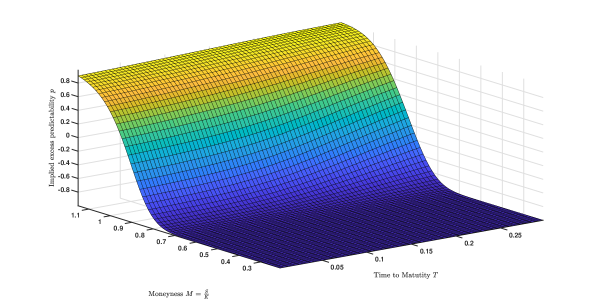
Figure 1: Implied dividend yield against time to maturity and moneyness.

Since implied excess predictability surfaces of all models are very similar, we plot the excess predictability surface when ${\sigma}_{t}$ is estimated from realized volatility. The implied excess predictability surface is graphed against both a standard measure of “moneyness” and time to maturity (in year) in Figure 1. Recall that a high value for $p$ (close to one) means excess predictability of SPY daily return traded by ${\beth}^{\left(s\right)}$ over the predictability of SPY traded by ${\beth}^{\left(l\right)}$. In other words, $p=1$ means that option traders potentially predict the future of the SPY returns better than the spot trader. The opposite is true when $p=-1$. Recall that the implied excess predictability surface is an increasing function of ${\sigma}_{t}$.

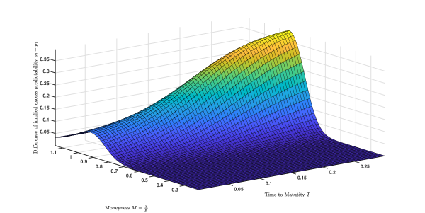
Figure 2: Relative difference of excess predictability VIX-Realized model against time to maturity and Moneyness.

Figure 1 indicates that at each maturity, implied excess predictability of option traders increase as moneyness increases. Where the moneyness varies in $(0,0.7)$, the surface is flat at point $-1$, indicating higher predictability of spot traders comparing to option traders. Thus, to price significant out-the-money options, the value of $p$ in the model should be $-1$. Where the moneyness varies in $(1.05,1.15)$, in-the-money options, the value of $p$ starts increasing from $0.5$, and flats out at point $1$. This finding indicates that option traders can potentially predict market changes better than spot traders when the option is in-the-money. In this case, for pricing in-the-money option, the value of $p$ in the log-return model should be $1$.

The turning point of the surface is where the moneyness is close to $0.95$. When the moneyness varies in $(0.90,1.05)$, $p$ varies in $(-0.5,0.5)$. This is the range that spot and option traders are equally informed about the market, and the predictability of the market is equal for both traders. Thus, to price options with no significant intrinsic value, the classical BSM equation can be used.

As we mentioned, the other four surfaces are very similar. Here, instead of plotting the four similar surfaces, we plot the relative difference of the excess predictability of each surface to the surface derived from realized variance, denoted by $p_{i}-p_{1}$, where $i=2,3,4$. Here (1) $p_{2}$ refers to the excess predictability surface when $\sigma_{t}$ is imputed from the VIX index, (2) $p_{3}$ is where $\sigma_{t}$ imputed by historical volatility, and (3) $p_{4}$ is where $\sigma_{t}$ is estimated by time series models. Figures 2-4 show the relative difference of excess predictability for each surface. In all surfaces, where the moneyness varies in $(0.90,1.05)$, the relative difference is significant. At each value for moneyness in $(0.90,1.05)$, the relative difference of excess predictability increases as time to maturity increases.

Zhou (2010) defined variance risk premium at time $t$ as the difference between the ex-ante risk-neutral expectation and the objective or statistical expectation of the return variance over the $[t,t+1]$ time interval,

$$VAR_{t}=E_{t}^{Q}(Var(r_{t+1}))-E_{t}^{P}(Var(r_{t+1})),$$ (18)

which is not directly observable in practice. In practice, the risk-neutral expectation of the return variance, $E_{t}^{Q}(Var(r_{t+1}))$, is typically replaced by the VIX² index and statistical expectation of the return variance, $E_{t}^{P}(Var(r_{t+1}))$, is estimated by realized variance.

Zhou (2010) showed that the difference between implied variance and realized variance ((i.e., variance risk premium) can be used for the short-term predictability of equity returns, bond returns, forward premiums, and credit spreads. Comparing Figures 2-4, the most significant relative difference of excess predictability is observed in Figure 2. It indicates that the VIX index contains more information about the stock market compared to the other metrics. Figure 3, the historical-realized surface, has the minimum relative difference.

Recall that the maximum and minimum values for $\sigma_{t}$ are derived from the VIX and realized volatility. As we observed, the most significant relative difference of excess predictability, Figure 2, is derived where the VIX and realized volatility are used in the model. Thus, by comparing equation (18) for different volatility measures and the fact that excess predictability is an increasing function of $\sigma_{t}$, suggests that the variance risk premium measure potentially contains more information compared to the other variance measures for predicting stock market returns. The historical volatility measure is the poorest metric.

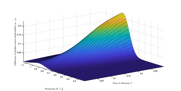
Figure 3: Relative difference of excess predictability Historical-Realized model against time to maturity and Moneyness.

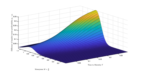
Figure 4: Relative difference of excess predictability time series-Realized model against time to maturity and Moneyness.

4 Conclusion

In this paper, we studied the predictability of stock returns within the framework of rational finance rather than relying on behavioral finance explanations. We proposed a method to model stock returns by incorporating the predictability of stock returns in the model and then deriving an option pricing formula. To compare the predictability of stock returns by option traders and spot traders, we constructed a forward-looking measure that compares the option and spot trader’s stock returns predictability which we called the “implied excess predictability measure.” The empirical results indicate that to price a significant in-the-money and out-the-money option, the option’s and spot trader’s predictability of stock returns should be incorporated into the BSM model. For options with a small intrinsic values, spot traders and option traders are equally informed, and the predictability of the market is equal for both traders. In this case, the classical BSM model can be used for option pricing without incorporating stock return predictability. Finally, we showed that the difference between implied variance and realized variance, which we called variance risk premium, is an informative measure for predicting the market in contrast to other volatility measures.

References

- Avramov (2003) Avramov, D. (2003). Stock return predictability and asset pricing models. Review of Financial Studies 17, 699–738.
- Barberis and Thaler (2003) Barberis, N. and R. Thaler (2003). A survey of behavioral finance. In G. Harris and R. Stulz (Eds.), Handbook of the Economics of Finance, Chapter 18, pp. 1051–1121. North Holland, Amsterdam: Elsevier Science.
- Bekiros (2013) Bekiros, S. D. (2013). Irrational fads, short-term memory emulation, and asset predictability. Review of Financial Economics 22, 213–219.
- Black and Scholes (1973) Black, F. and M. Scholes (1973). The pricing of options and corporate liabilities. Journal of Political Economy 81, 637–654.
- Campbell and Shiller (1988) Campbell, J. Y. and R. J. Shiller (1988). The dividend-price ratio and expectations of future dividends and discount factors. Review of Financial Studies 1(3), 195–228.
- Daniel and Hirshleifer (2015) Daniel, K. and D. Hirshleifer (2015). Overconfident investors, predictable returns, and excessive trading. Journal of Economic Perspectives 29, 61–88.
- Duffie (2001) Duffie, D. (2001). Dynamic Asset Pricing Theory, 3rd Edition. Princeton University Press: Princeton N.J.
- Fama and French (1988) Fama, F. E. and R. K. French (1988). Dividend yields and expected stock returns. Journal of Financial Economics 22, 3–25.
- Ferson (2006) Ferson, W. E. (2006). Conditional asset pricing. In A. C. Lee (Ed.), Encyclopedia of Finance, Chapter 9, pp. 376–383.
- Huang et al. (2009) Huang, Y. C., C. W. Wu, and C. W. Wang (2009). Valuing american options under ARMA processes. International Research Journal of Finance and Economics 28, 152– 159.
- Kandel and Stambaugh (1996) Kandel, S. and R. F. Stambaugh (1996). On the predictability of stock returns: An asset-allocation perspective. Journal of Finance 51, 385–424.
- Kloeden et al. (2000) Kloeden, P. E., E. Platen, and H. Schurz (2000). Numerical Solution of SDE Through Computer Experiments. Heidelberg: Springer-Verlag.
- Kumar and Chaturvedul (2013) Kumar, K. and C. Chaturvedul (2013). Price leadership between spot and futures markets. Journal of Applied Finance and Banking 3(1), 93–107.
- Lewellen (2000) Lewellen, J. W. (2000). On the Predictability of Stock Returns: Theory and Evidence. Ph. D. thesis, William E. Simon Graduate School of Business Administration, University of Rochester.
- Liao and Chen (2006) Liao, S. L. and C. C. Chen (2006). The valuation of European options when asset returns are autocorrelated. Journal of Futures Markets 26(1), 85–102.
- Lo and Wang (1995) Lo, A. W. and J. Wang (1995). Implementing option pricing models when asset returns are predictable. Journal of Finance 50(1), 87–129.
- Malkiel (2003) Malkiel, B. G. (2003). The efficient market hypothesis and its critics. Journal of Economic Perspectives 17, 59–82.
- Merton (1973) Merton, R. C. (1973). Theory of rational option pricing. Bell Journal of Economics and Management Science, 6, 141–183.
- Neely and Weller (2000) Neely, C. J. and P. Weller (2000). Predictability in international asset returns: A reexamination. Journal of Financial and Quantitative Analysis 35, 601–620.
- Øksendal (2003) Øksendal, B. K. (2003). Stochastic Differential Equations: An Introduction with Applications. Heidelberg: Springer-Verlag.
- Paschke and Prokopczusk (2010) Paschke, R. and M. Prokopczusk (2010). Commodity derivative valuation with autoregressive and moving average components in the price dynamics. Journal of Banking and Finance 34, 2742–2752.
- Peleg (2000) Peleg, E. (2000). Three essays on asset pricing, portfolio choice and behavioral finance. Ph. D. thesis, Philosophy in Management, University of California.
- Pesaran (2010) Pesaran, M. H. (2010). Predictability of asset returns and the efficient market hypothesis. In A. Ullah and D. E. Giles (Eds.), Handbook of Empirical Economics and Finance, Chapter 11, pp. 281–31. North Holland, Amsterdam: Elsevier Science.
- Shiller (2003) Shiller, R. J. (2003). From efficient market theory to behavioral finance. Journal of Economic Perspectives 17, 83–104.
- Shirvani et al. (2019) Shirvani, A., S. Rachev, and F. Fabozzi (2019). Multiple subordinated modeling of asset returns. arXiv:1907.12600 [q-fin.MF] 7.
- Syga (2015) Syga, J. (2015). Semimartingale measure in the investigation of Stratonovich-type stochastic integrals and inclusions. Discussiones Mathematicae, Probability and Statistics 35, 7–27.
- Wachter and Warusawitharana (2009) Wachter, J. A. and M. Warusawitharana (2009). Predictable returns and asset allocation: Should a skeptical investor time the market? Journal of Econometrics 148, 162–178.
- Zhou (2010) Zhou, H. (2010). Variance risk premia, asset predictability puzzles, and macroeconomic uncertainty. Annual Review of Financial Economics 10(1), 481–497.