Critical Phenomena of Dynamical Delocalization in Quantum Maps: standard map and Anderson map

Abstract

Following the paper exploring the Anderson localization of monochromatically perturbed kicked quantum maps [Phys.Rev. E97,012210], the delocalization-localization transition phenomena in polychromatically perturbed quantum maps (QM) is investigated focusing particularly on the dependency of critical phenomena upon the number $M$ of the harmonic perturbations, where $M+1=d$ corresponds to the spatial dimension of the ordinary disordered lattice. The standard map and the Anderson map are treated and compared. As the basis of analysis, we apply the self-consistent theory (SCT) of the localization, taking a plausible hypothesis on the mean-free-path parameter which worked successfully in the analyses of the monochromatically perturbed QMs. We compare in detail the numerical results with the predictions of the SCT, by largely increasing $M$. The numerically obtained index of critical subdiffusion $t^{\alpha}$ ($t$:time) agrees well with the prediction of one-parameter scaling theory $\alpha=2/(M+1)$, but the numerically obtained critical exponent of localization length significantly deviates from the SCT prediction. Deviation from the SCT prediction is drastic for the critical perturbation strength of the transition: if $M$ is fixed the SCT presents plausible prediction for the parameter dependence of the critical value, but its value is $1/(M-1)$times smaller than the SCT prediction, which implies existence of a strong cooperativity of the harmonic perturbations with the main mode.

I Introduction

It is a basic nature of the freely propagating quantum particle that it localizes by inserting random impurities anderson58 ; ishii73 and its normal conduction, which is an irreversible quantum Brownian motion, is realized after destroying the localization by some additional operations. The ordinary way to free from localization is to increase the spatial dimension of the system and weaken the randomness. An another way is to introduce dynamical perturbations such as harmonic vibrations due to the lattice vibration. The destruction of localization by the latter way is called dynamical delocalization. The purpose of the present paper is to elucidate the critical phenomena of the dynamical localization-delocalization transition (LDT) numerically and theoretically, following previous papers yamada15 and yamada18 . (We referred to them as [I] and [II], respectively, in the text.) Recently the localization and delocalization of wavepacket propagation has been investigated experimentally and theoretically. In particular, the quantum standard map (SM) systems, which theoretically shown to exhibit dynamical localization casati79 , has been studied extensively. If SM is coupled with dynamical harmonic perturbations composed of $M$ incommensurate frequencies, it can formally be transformed into a $d(=M+1)-$dimensional lattice system with quasi-periodic potential casati89 ; borgonovi97 ; chabe08 ; wang09 ; lemarie10 ; tian11 . Then it can be expected that the harmonically perturbed SM will undergo a Anderson transition of the $d(=M+1)-$dimensional random quantum lattice.

Indeed, Lopez et al implemented the perturbed SM as a cold atom on the optical lattice, and succeeded in observing the Anderson transition lopez12 ; lopez13 . They obtained the critical diffusion exponents and the critical localization exponents experimentally, which agreed with numerical and theoretical results for $M=2$. They also observed an exponentially exteded localization for $M=1$ manai15 .

We can then expect that even the localization phenomenon on low-dimensional disordered quantum lattice can be also delocalized by applying harmonic perturbations with finite number of incommensurate frequency components yamada98 ; yamada99 . The increment of the number $M$ of the frequencies will make the delocalization easier, thereby realizing the onset of diffusion which is a typical irreversible motion simulating the normal conduction of electron. To examine the above conjecture, we proposed a quantum map defined on a disordered lattice, which we call the Anderson map (AM) yamada04 . It evolves in a discretized time and become the one-dimensional disordered system in a continuous time limit.

The SM of $M=1$ corresponds to the asymmetric two-dimensional disordered system, and the localization length is exponentially enhanced but the LDT does not occur, which has been confirmed experimentally and numerically manai15 . In the previous paper [II]yamada18 we also numerically and theoretically studied the localization characteristics of AM of $M=1$ in comparison with that of the SM of $M=1$, and all the numerical results were well explained in terms of the self-consistent theory (SCT) of the localization wolfle10 . The AM of $M=1$ has a paradoxical character that the localization length increases as the disorder strength $W$ of potential exceeds a threshold value $W^{*}$, which was successfully predicted by the SCT.

On the other hand, we presented a preliminary paper [I] in which we showed that the AM with $M\geq 2$ undergoes the LDT as is the case of the SM with $M\geq 2$ and further the results based upon the one-parameter scaling hypothesis can explain the critical diffusion exponent for a wide range of $M$ yamada15 .

The present paper provides a complete numerical and theoretical analysis of the localization-delocalization characteristics of AM in comparison with SM for a wide range of control parameters, particularly, with changing $M$ largely.

In Sect.II, we introduce polychromatically perturbed quantum standard map (SM) and Anderson map (AM). First, in Sect.III we begin with reviewing the results reported by the papers [I] and paper [II] about the $M$ dependency of the critical subdiffusion exponent and the critical localization exponent, including some new results. We are particularly interested in the dependencies of the critical perturbation strength of the harmonic perturbation (we denote it by $\epsilon_{c}$ hereafter) on the control parameters of the system and the predictability of the SCT for them. We show in Sect.IV the theoretical prediction based on SCT for critical perturbation strength $\epsilon_{c}$ of the LDT for SM and AM and compare them with the numerical results. Except for $M$, the SCT successfully predicts the dependency of $\epsilon_{c}$ upon the control parameters. However, the SCT fails to predict the $M-$dependence. Numerically, it turns out that $\epsilon_{c}\simeq 1/(M-1)$ for both AM and SM, but the SCT predicts that it is a constant. In Sect.V, we summarize and discuss the result. The derivation of some equations and some details of the numerically decided critical exponent of the localization are given in appendixes.

II Models and their dynamics

We consider dynamics of the following quantum map systems represented by the Hamiltonian,

$$H_{tot}(\hat{p},\hat{q},t)=T(\hat{p})+V(\hat{q},\{\omega_{j}t\})\delta_{t},$$ (1)

where $\delta_{t}=\sum_{k=-\infty}^{\infty}\delta(t-k\Delta)$. In this paper we set the period of the kicks $\Delta=1$. $T(\hat{p})$ is the kinetic energy term, and the potential energy term $V(\hat{q},t)$ including time dependent perturbation $f(t)$ is given as,

$$V(\hat{q},\{\omega_{j}t\}) = V(\hat{q})[1+f(\{\omega_{j}t\})]$$ (2)

$$= V(\hat{q})\left[1+\frac{\epsilon}{\sqrt{M}}\sum_{j}^{M}\cos(\omega_{j}t)\right],$$ (3)

where $M$ and $\epsilon$ are number of the frequency component and the strength of the perturbation, respectively. Note that the strength of the perturbation is divided by $\sqrt{M}$ so as to make the total power of the long-time average independent of $M$, i.e. $\overline{f(\{\omega_{i}t\})^{2}}=\epsilon^{2}/2$, and the frequencies $\{\omega_{j}\}(j=1,...,M)$ are taken as mutually incommensurate number of $O(1)$. Here $\hat{p}$ and $\hat{q}$ are momentum and position operators, respectively.

In the present paper, we use the standard map (SM), which is given by,

$$T(\hat{p})=\frac{p^{2}}{2},~{}~{}V(\hat{q})=v(\hat{q}).$$ (4)

In addition, we deal with Anderson map (AM), which is given by,

$$T(\hat{p})=2\cos(\hat{p}/\hbar),~{}~{}V(\hat{q})=Wv(\hat{q}),$$ (5)

where

$$v(\hat{q})=\begin{cases}K\cos\hat{q}&{\rm(for~{}SM)}\\ \sum_{n\in{\mathbb{Z}}}\delta(q-n)v_{n}|n\rangle\langle n|&{\rm(for~{}AM)}.\end{cases}$$ (6)

In the case of SM the global propagation occurs in the momentum space $p$ spanned by the momentum eigenstates $|p\rangle=|P\hbar\rangle~{}~{}(P\in{\mathbb{Z}})$, being transferred by the potential operator $v(\hat{q})$. On the other hand, in the case of AM $v(\hat{q})$ plays the role of the on-site potential operator taking random value $v_{n}$ uniformly distributed over the range $[-1,1]$, and $W$ denotes the disorder strength. The global propagation occurs in the position space $q$, which are spanned by the position eigenstates $|n\rangle~{}(n\in{\mathbb{Z}})$ yamada10 . The AM is a quantum map with discretized time but it approaches to the time-continuous Anderson model defined on the random lattice for $W\ll 1$.

We can regard the harmonic perturbations as the dynamical degrees of freedom. To show this we introduce the classically canonical action-angle operators $(\hat{J}_{j}=-i\hbar\frac{\partial_{j}}{\partial\phi_{j}},\phi_{j})$ representing the harmonic perturbation as a linear mode (we call the “harmonic mode” hereafter) and extend the Hamiltonian (1) so as to include the harmonic modes,

$$H_{aut}(\hat{p},\hat{q},\{\hat{J}_{j}\},\{\hat{\phi}_{j}\})$$

$$~{}~{}~{}~{}~{}~{}=T(\hat{p})+V(\hat{q},\hat{\phi},\{\hat{\phi}_{j}\})\delta_{t}+\sum_{j=1}^{M}\omega_{j}\hat{J}_{j},$$ (7)

where

$$V(\hat{q},\{\hat{\phi}_{j}\}) = V(\hat{q})[1+f(\{\hat{\phi}_{j}\})],$$

$$= V(\hat{q})\left[1+\frac{\epsilon}{\sqrt{M}}\sum_{j}^{M}\cos\phi_{j}\right].$$

One can easily check that by Malyland transform the eigenvalue problem of the quantum map system interacting with $M$-harmonic modes can be transformed into $d(=M+1)-$dimensional lattice problem with quasi-periodic and/or random on-site potentials fishman82 ; yamada18 . (See appendix A.) In this view, to increase the number of the harmonic modes is to increase the dimension of the system, which enables the LDT.

From the dynamical point of view, the harmonic modes perturbs the main mode to cause the diffusive motion and induce the LDT. On the other hand, by the backaction of the perturbation to the main mode, the harmonic mode is excited to propagate along the ladder of action eigenstates satisfying $\hat{J}_{j}|m_{j}\rangle=m_{j}\hbar|m_{j}\rangle~{}(m_{j}\in{\mathbb{Z}}$). Let $\hat{y}_{j}=\hat{J}_{j}/\hbar=\sum_{m_{i}\in{\mathbb{Z}}}m_{i}|m_{i}\rangle\langle m_{i}|$ be the operator indicating the excitation number in the action space, then the Heisenberg equation of motion $d\hat{y}_{j}/dt\hbar=(i/\hbar^{2})[H_{aut},\hat{J}_{j}]=-1/\hbar\partial V(\hat{q},\{\phi_{j}\})/\partial\phi_{j}$ gives the step-by-step evolution rule for the Heisenberg operators:

$$\hat{y}_{j}(t)-\hat{y}_{j}(0)=\frac{\epsilon}{\sqrt{M}}\sum_{s=0}^{t}C_{j}\hat{G}(s)\sin(\omega_{j}s+\phi_{j0}),$$ (9)

where $\phi_{j0}$ is the initial phase. Here,

$$\hat{G}(t)=\frac{1}{\hbar}v(\hat{q}(t))$$ (10)

and

$$C_{j}=\begin{cases}1~{}~{}~{}{\rm~{}~{}(for~{}SM)},\\ W~{}~{}{\rm~{}~{}(for~{}AM)}.\end{cases}$$ (11)

The potential $v(\hat{q}(t))$ works as a force inducing a propagation along the action ladder.

To treat the transport in the main mode of SM and AM in a unified manner, we define the excitation number operator in the momentum space $\hat{x}=\hat{p}/\hbar=\sum_{P}P|P\hbar\rangle\langle P\hbar|~{}~{}(P\in{\mathbb{Z}})$ for SM and in the real space $\hat{x}=\sum_{n}n|n\rangle\langle n|~{}(n\in{\mathbb{Z}})$ for AM, where $|P\hbar\rangle$ and $|n\rangle$ are the momentum and the real position eigenstates, respectively. Then the step-by-step evolution rule for the Heisenberg operator is

$$\hat{x}(t)-\hat{x}(0)=\sum_{s=0}^{t}\hat{F}(s),$$ (12)

where the force $\hat{F}$ is

$$\hat{F}(t)=\begin{cases}\frac{K}{\hbar}\sin\hat{q}(t)~{}~{}&{\rm(for~{}SM)}\\ -\frac{2}{\hbar}\sin(\hat{p}(t)/\hbar)~{}~{}&{\rm(for~{}AM)}.\end{cases}$$ (13)

In the next section, with the basic formal representations presented above, we first discuss the localization of unperturbed SM and AM and further the transition to the delocalized states.

III Critical subdiffusion of LDT in the polychromatically perturbed quantum maps

In this section we show the results related to the critical subdiffusion which is a remarkable feature of the critical state of the LDT, by organizing the known results reported in the previous papers yamada18 ; yamada15 and the new ones.

III.1 Localization in the unperturbed and monochromatically perturbed quantum maps ($M=0,1$)

We use an initial quantum state $|\Psi(t=0)\rangle$ and the $x-$representation $\langle x|\Psi(t=0)\rangle=\delta_{x,N/2}$ and characterize quantitatively the spread of the wavepacket by the mean square displacement (MSD),

$$m_{2}(t) = \langle\Psi(t=0)|(\hat{x}(t)-\hat{x}(0))^{2}|\Psi(t=0)\rangle$$ (14)

$$\equiv \langle(\hat{x}(t)-\hat{x}(0))^{2}\rangle,$$

where $\hat{x}$ is $\hat{p}$ for SM and $\hat{x}$ is $\hat{q}$ for AM, respectively. Using Eq.(12), it immediately follows that

$$m_{2}(t)=\sum_{s\leq t}D^{(0)}_{0}(s:t),$$ (15)

where

$$D^{(0)}_{0}(s:t)=\sum_{s^{{}^{\prime}}=s}^{t}\langle\hat{F}(s)\hat{F}(s^{{}^{\prime}})\rangle+c.c.$$ (16)

In the unperturbed 1D quantum maps with $\epsilon=0$, the time-dependent diffusion constant $D^{(0)}_{0}(s:t)$, which converges to a positive finite value $D^{(0)}_{0}$ if $s$ is small and $t\to\infty$, finally goes to zero as $s$ increases, and thus $m_{2}(t)$ given by Eq.(15) saturates and the wavepacket become localized in the limit $t\to\infty$. Let the localization length and the time scale beyond which the diffusion terminates be $\ell_{0}$ and $t_{0}$, respectively, then Eq.(15) gives $\ell_{0}^{2}=m_{2}(\infty)\sim D^{(0)}_{0}t_{0}$, where $D^{(0)}_{0}:=D^{(0)}_{0}(0:\infty)$ is the initial stage diffusion constant which converges to a positive finite value.

In the localized phase, in the spatial region of localization length $\ell_{0}$ all the localized eigenfunctions of number $\ell_{0}$ supported by the region undergo very strong level repulsion. The interval between the nearest neighbouring eigenangles should be $\sim 1/\ell_{0}$, which means that its inverse ($\sim\ell_{0}$) characterizes the localization time $t_{0}$. Then the relation means that

$$\ell_{0}^{2}\sim D^{(0)}_{0}\ell_{0},$$ (17)

and therefore

$$D^{(0)}_{0}\sim\ell_{0}\sim t_{0}$$ (18)

the localization length as well as the localization time are decided by the diffusion constant. One can confirm that the SCT discussed later also supports the above relation if it is applied to the isolated (i.e., $\epsilon=0$) one-dimensional system. In the case of isolated SM, $D^{(0)}_{0}$ equals to the classical chaotic diffusion constant casati84 :

$$D^{(0)}_{0}\sim\ell_{0}\sim D_{cls}/\hbar^{2}~{}~{}\to K^{2}/\hbar^{2}~{}(K^{2}\gg 1)$$ (19)

On the other hand, in the case of the isolated AM, the well-known result $\ell_{0}\sim 1/W^{2}$ for the continuous-time Anderson model holds lifshiz88 . However, this result holds correct only for $W$ less than the characteristic value decided by

$$W^{*}\sim 2\pi\hbar,$$ (20)

beyond which $\ell_{0}$ terminates to decrease and approaches to a constant $\sim 1/W^{*2}$ yamada18 . This is a remarkable feature of the AM different from the continuous-time Anderson model. Then, we have

$$D^{(0)}_{0}\sim\ell_{0}\sim\begin{cases}&1/W^{2}~{}~{}~{}~{}(W\ll W^{*})\\ &1/W^{*2}~{}~{}~{}(W\gg W^{*}).\end{cases}$$ (21)

A basic hypothesis assumed here is that the temporal localization process of isolated system starts with a transient diffusion process with the diffusion constant $D^{(0)}_{0}$. As will be discussed later this hypothesis does not work in a certain case of AM, but we first use this hypothesis in the next section. As is shown in the appendix A, the eigenvalue problem of our systems, which are represented as $M+1$ degrees of freedom system in the extended scheme of Eq.(7), is formally transformed into $d(=M+1)-$dimensional lattice problem with quasi-periodic and/or random on-site potentials by the so-called Maryland transform. As was demonstrated in the paper [I] the delocalization transition do not occur for $M=1$, i.e., for the effective dimension $d=2$, although the localization length grows exponentially as $\ell_{0}\propto{\rm e}^{{\rm const.}\epsilon}$. We thus consider the case $M(=d-1)\geq 2$, for which the LDT may take place according to the ordinary scenario of Anderson transition.

III.2 $M-$dependence of subdiffusion in SM and AM ($M\geq 2$)

As partially shown in the paper [II], the perturbation strength $\epsilon$ exceeds the critical value $\epsilon_{c}$ the LDT occurs if $M\geq 2$.

In the LDT an anomalous diffusion

$$m_{2}\sim t^{\alpha}(0<\alpha<1).$$ (22)

with the characteristic exponent $\alpha$ is observed at the critical perturbation strength $\epsilon=\epsilon_{c}$.

The presence of subdiffusion is confirmed in the preliminary report [II], and a more detailed study of the critical subdiffusion for control parameters covering much wider regime is executed. It is convenient to define the scaled MSD $\Lambda(t)$ divided by the critical subdiffusive factor in order to investigate the critical behavior close to LDT:

$$\Lambda(t)=\frac{m_{2}(t)}{t^{\alpha}}.$$ (23)

This scaled MSD is also used in finite-time scaling to determine the critical exponent of LDT. (See appendix C.)

We first show the case of SM. Figure 2(a) and (c) show the time-dependence of MSD $m_{2}(t)$ in the cases of $M=3$ and $M=7$, respectively, for various values of $\epsilon$ increasing across the critical value $\epsilon_{c}$. Figure 2 (b) and (d) show the scaled MSD $\Lambda(t)$ corresponding to (a) and (c). It can be seen that a transition from the localized state to the delocalized state occurs going through a stable subdiffusion state as $\epsilon$ increases. The scaled MSD $\Lambda(t)$ also shows a very characteristic holding-fan-pattern whose behavior leads to a remarkable scaled behavior with respect to the critical parameter $|\epsilon-\epsilon_{c}|$.

Figure 2(a) shows the critical subdiffusions at the critical point $\epsilon=\epsilon_{c}$ when the color number $M$ is changed. It is evident that the diffusion index $\alpha$ at the critical point $\epsilon_{c}$ decreases as $M$ increases, and the numerical results tell that it can be approximated very well by the rule

$$\alpha\simeq\frac{2}{M+1},$$ (24)

regardless of the values of the control parameters such as $K$ and $\hbar$. The result is also consistent with the well-known guess based upon the one-parameter scaling theory (OPST) of the localization, which are summarized in appendix B. The critical value $\epsilon_{c}$ decreases with $M$ as well as $\alpha$, which will be discussed in detail in next section.

*       

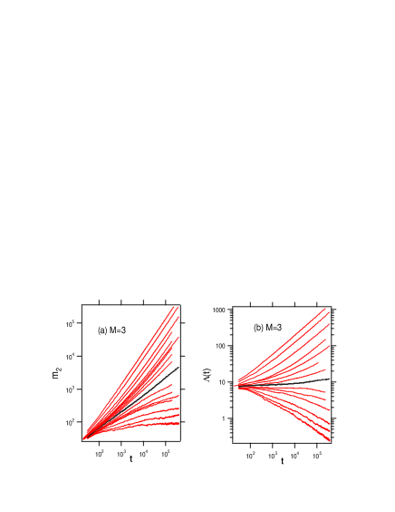
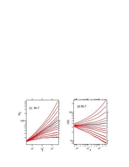
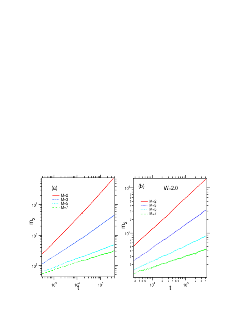
Figure 1: (Color online) The double-logarithmic plots of (a)$m_{2}(t)$ and (b)the scaled $\Lambda(\epsilon,t)$ as a function of time for different values of the perturbation strength $\epsilon$, where the diffusion exponent $\alpha$ is determined by the least-square-fit for the $m_{2}(t)$ with the critical case, in the polychromatically perturbed SM of $M=3$ with $K=3.1$, $\hbar=2\pi\times 311/2^{13}(\equiv\hbar_{0})$. (c)The same $m_{2}(t)$ and (d)the scaled $\Lambda(\epsilon,t)$ in the polychromatically perturbed SM of $M=7$. In the case of $M=3$, $\epsilon_{c}^{SM}\simeq 0.0081$, $m_{2}\sim t^{\alpha}$ with $\alpha\simeq 0.46$. In the case of $M=7$, $\epsilon_{c}^{SM}\simeq 0.012$, $m_{2}\sim t^{\alpha}$ with $\alpha\simeq 0.25$. The data near the critical value $\epsilon_{c}$ are shown by bold black lines. In the following we representation $\hbar=\hbar_{0},2\hbar_{0},3\hbar_{0},...$ as an unit $\hbar_{0}=2\pi\times 311/2^{13}\simeq 0.24$.

Figure 2: (Color online) The double-logarithmic plots of $m_{2}(t)$ as a function of time near the critical pints $\epsilon_{c}$ in (a) the polychromatically perturbed SM ($M=2,3,5,7$) with $K=3.1$, $\hbar=\hbar_{0}$, and (b) AM ($M=2,3,5,7$) with $W=2.0$. In the perturbed SM and AM, the system and ensemble sizes are $N=2^{15}\sim 2^{17}$ and $10\sim 100$, respectively, throughout this paper.

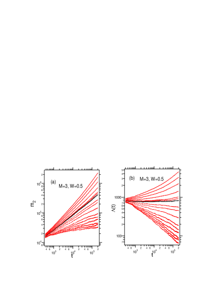
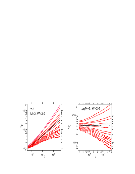
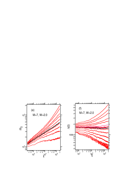
Figure 3: (Color online) The double-logarithmic plots of (a)$m_{2}(t)$ and (b)the scaled $\Lambda(\epsilon,t)$ as a function of time for different values of the perturbation strength $\epsilon$, where the diffusion exponent $\alpha$ is determined by the least-square-fit for the $m_{2}(t)$ with the critical case, in the trichromatically perturbed AM of $M=3$ with $W=0.5$ (c)The same $m_{2}(t)$ and (d)the scaled $\Lambda(\epsilon,t)$ in the trichromatically perturbed AM of $M=3$ with $W=2.0$. (e)The same $m_{2}(t)$ and (f)the scaled $\Lambda(\epsilon,t)$ in the trichromatically perturbed AM of $M=7$ with $W=2.0$. In the case $M=3$ with $W=0.5$, $\epsilon_{c}^{AM}\simeq 0.038$, $\alpha\simeq 0.5$. In the case $M=3$ with $W=2.0$, $\epsilon_{c}^{AM}\simeq 0.011$, $\alpha\simeq 0.5$. In the case $M=7$ with $W=2.0$, $\epsilon_{c}^{AM}\simeq 0.0068$, $\alpha\simeq 0.25$. We take $\hbar=0.125$ as the Planck constant for the perturbed AM. The data near the critical value $\epsilon_{c}$ are shown by bold black lines.

Next we show the corresponding observations for AM. Fig.3 shows the dynamic behavior of AM near the LDT. According to Eq.(21), the disorder strength $W$ of AM has the characteristic value $W^{*}$ beyond which localization characteristics change. At fixed $M=3$, the time-dependence of $m_{2}(t)$ and $\Lambda(t)$ for $W=0.5(<W^{*})$ and $W=2.0(>W^{*})$ are shown in Fig. 3(a),(b) and (c),(d), respectively, for various values of $\epsilon$ increased across the critical value $\epsilon=\epsilon_{c}$ of LDT. It follows that the LDT occurs regardless of the value of $W$. The result for $M=7$ is also displayed in Fig.3(e)(f). As with the SM, we can see the existence of the LDT and the critical subdiffusion with increasing $\epsilon$. The critical subdiffusion index $\alpha$ of AM also obeys the “universal rule” Eq.(24) and moreover the critical value $\epsilon_{c}$ depends on $M$ in the same way as the SM. However the dependence of $\epsilon_{c}$ on the randomness parameter $W$ changes at $W=W^{*}$. These properties will be discussed later in detail.

In the following, the characteristics of LDT are studied changing the values of control parameters in a wide range. In SM, we study the change in critical behavior for parameter $K$ that controls classical chaos, and Planck constant $\hbar$ that controls quantum property, whereas AM uses parameter $W$ that controls randomness. In AM, the size of $\hbar$ is kept at $O(1)$. The parameters $K$, $\hbar$ and $W$ are important because they decides the localization length $\ell_{0}$ by Eqs.(19) and (21).

However, in the present study the dependency of LDT on the number of the harmonic degrees of freedom $M$ is of particular interest. Indeed, the change of $M$ is reflected significantly in the characteristics of critical subdiffusion index by Eq.(24), which should also be reflected in $\epsilon_{c}$.

We are also interested in critical exponents characterizing the divergence of localization length close to the critical point, but it have been fully discussed in the previously published paper [II]. Some extensive arguments for this topic is presented in the appendix C.

IV Critical coupling strength of LDT in the polychromatically perturbed quantum maps

We focus our attention to the critical value $\epsilon_{c}$ of LDT, which is investigated numerically and compared with theoretical prediction based upon the SCT. This is the main part of the present paper.

IV.1 A prediction based on self-consistent theory

The critical perturbation strength $\epsilon_{c}$ is a quite important parameter featuring the LDT. The one parameter scaling theory, which is very powerful for the prediction of critical exponents, is not applicable to evaluate the critical point. We use here the SCT for predicting the characteristics of $\epsilon_{c}$.

Let $j=0$ assign to the main degrees of freedom of SM and AM, and $j=1,..,M$ to the $M$ harmonic modes. We regard our systems as $(M+1)-$degrees of freedom one according to Eqs.(A) and (A), which can be identified with a $d(=M+1)-$dimensional lattice with random and$/$or quasi-periodic on-site potential as is shown in appendix A. Then we can apply the scheme of SCT for the $d-$dimensional disordered lattice system to our system. Let the frequency-dependent diffusion constant of the $j$-mode be $D_{j}(\omega)$. The ratio of $D_{j}(\omega)$ to the bare diffusion constant $D^{(0)}_{j}$ is reduced from 1 by the correction due to the coherent backward scattering, satisfying the relation

$$\frac{D_{j}(\omega)}{D^{(0)}_{j}}=1-C\frac{D_{j}(\omega)}{D^{(0)}_{j}}\int^{q_{0}^{c}}...\int^{q_{d-1}^{c}}\prod_{k=0}^{d-1}dq_{k}\frac{1}{-i\omega+\sum_{k=0}^{d-1}D_{k}(\omega)q_{k}^{2}},$$ (25)

where $C$ is a constant value independent of the parameters. Note that the integral over $q_{k}$ has a cutoff $q_{k}^{c}$, which plays a crucial role yamada18 . If we set

$$\frac{D_{j}(\omega)}{-i\omega}=\xi_{j}(\omega)^{2},$$ (26)

then $\lim_{\omega\to 0}\xi_{j}(\omega)=\ell_{j}$ becomes the localization length. In the limit of $\epsilon=0$, the propagation along the mode $j$ terminates at the localization length $\ell_{j}$. We suppose that the inverse of $\ell_{j}$ decide the cut-off wavenumber $q_{k}^{c}$, i.e.,

$$q_{j}^{c}\sim\ell_{j}^{-1},$$ (27)

which correctly predicts numerical results of the localization process in the case of $M\leq 2$ yamada18 . As the localization length of the main mode $j=0$ we take $\ell_{0}$ of Eqs.(19) and (21), then Eq.(18) holds and $\ell_{0}=D^{(0)}_{0}$. The diffusion along the harmonic mode $j$ occurs according to Eq.(9), being driven by the force $\hat{G}(t)$. Similarly to Eq.(15), the MSD of the harmonic mode $j$ grows as

$$\left<(\hat{y}(t)-\hat{y}(0))^{2}\right>=\sum_{s\leq t}D^{(0)}_{j}(s:t),$$ (28)

where

$$D^{(0)}_{j}(s:t)=$$

$$~{}C_{j}^{2}\frac{\epsilon^{2}}{2M}\sum_{s^{\prime}=s}^{t}\langle\hat{G}(s^{\prime})\hat{G}(s)\rangle\cos(\omega_{j}(s^{\prime}-s))+c.c,$$ (29)

where the average over the initial phase $\phi_{j0}$ is done.

In the case of SM, the force driving the diffusion of the main mode $\hat{F}(t)\propto\sin\hat{q}$ (Eq.(15)) has the same correlation property as that of the harmonic mode $\hat{G}(t)\propto\cos\hat{q}$. For AM, we also use the same assumption that the driving force for the harmonic mode ($\hat{G}(t)=\sum_{n}v_{n}|n\rangle\langle n|/\hbar~{}~{}(|v_{n}|\sim O(1))$) and that for the main mode ($\hat{F}(t)=2\sin(\hat{p}/\hbar)/\hbar=\sum_{n}(|n\rangle\langle n+1|-|n+1\rangle\langle n|)/(i\hbar)$) has the same correlation property. Then following the idea of deriving Eq.(17), the diffusion of the harmonic mode terminates at the localization time $t_{0}=\ell_{0}$ of the main mode and so the localization length of the mode $j$ is

$$\ell_{j}^{2}=D^{(0)}_{j}\ell_{0}$$ (30)

by using the initial stage diffusion constant $D^{(0)}_{j}:=D^{(0)}_{j}(s=0,t=\infty)$ of the $j$-mode. Let us define $\kappa_{j}(\omega):=\frac{\xi_{j}(\omega)}{\ell_{j}}$ which is the ratio of the enhanced localization length to the localization length. Then in the self-consistent equation (25) the only $j$ dependent parameter is $D_{j}(\omega)/D^{(0)}_{j}$, which is rewritten by using Eqs.(25) and (30) as

$$\frac{D_{j}(\omega)}{D^{(0)}_{j}}=-i\omega\kappa_{j}(\omega)^{2}\ell_{0}.$$

In order that all the equations for $j=0,1,...,d-2,d-1(=M)$ in Eq.(25) are consistent, $\kappa_{j}(\omega)$ should be equal and independent of $j$. By rescaling $q_{k}^{\prime}=q_{k}\xi_{k}(\omega)$, the integral of Eq.(25) can be approximated as the $d$-dimensional spherical integral over the radius $\kappa_{k}=\kappa_{0}$. If $\kappa(\omega)$ is much greater than unity assuming that $\epsilon$ is close to the critical point, Eq.(25) is integrated as

$$\frac{D_{j}(\omega)}{D^{(0)}_{j}} = 1-\frac{CS_{d}}{(d-2)\prod_{k=1}^{d-1}\ell_{k}}.$$ (31)

$S_{d}$ denotes the surface area of the $(d+1)$-dimensional sphere of radius unity:

$$S_{d}=\frac{2\pi^{d/2}}{\Gamma(\frac{d}{2})}.$$ (32)

According to Eq.(28) the diffusion constant $D^{(0)}_{j}$ of the $j(\neq 0)$-mode is the product of the factor $\frac{\epsilon^{2}}{2M}C_{j}^{2}$ and the time-integral of the correlation function of $\hat{G}$, which is the same as that of the driving force $\hat{F}$ of the main mode, as discussed above. Therefore, the diffusion constant of the $j(\neq 0)$mode is related to that of the main mode as

$$D^{(0)}_{j}=\frac{\epsilon^{2}}{2M}C_{j}^{2}D^{(0)}_{0}.$$ (33)

Note that $D^{(0)}_{0}$ is the diffusion constant of isolated main mode independent of $\epsilon$ and $M$.

The critical coupling strength $\epsilon_{c}$ which makes the l.h.s. of Eq.(31) zero is given as the condition for the harmonic mode $j\neq 0$ as follows:

$$\ell_{j}=\left[\frac{CS_{M+1}}{(M-1)}\right]^{1/M}.$$ (34)

From Eqs.(30) and (33) $\ell_{j}$ is proportional to $\epsilon\ell_{0}$, and the critical coupling strength is

$$\epsilon_{c}=\frac{c_{M}}{\ell_{0}C_{j}},$$ (35)

where the parameter $M$ is contained in $c_{M}=[CS_{M+1}/(M-1)]^{1/M}\sqrt{2M}$. If $M\gg 1$ the factor $1/\sqrt{M}$ in $c_{M}$ cancels with $M^{1/2}$ coming from the $(M+1)$-dimensional spherical surface area $S_{M}$, and $\epsilon_{c}$ does no longer depends upon $M$. This prediction will be compared with the numerical results.

In the case of SM the critical coupling strength is given from Eq.(19):

$$\epsilon_{c}^{SM}\sim 1/\ell_{0}\sim\hbar^{2}/D_{cls}\sim\left(\frac{K}{\hbar}\right)^{-2}~{}~{}(K\gg 1),$$ (36)

whereas, in the case of AM, following Eq.(21), the critical value changes its dependency upon $W$ at $W=W^{*}$:

$$\epsilon_{c}^{AM}\sim 1/(\ell_{0}C_{j})\sim\begin{cases}W~{}~{}~{}~{}~{}~{}(W<W^{*}),\\ \dfrac{W^{*2}}{W}~{}~{}~{}(W>W^{*}).\end{cases}$$ (37)

All the above results are the predictions of the SCT.

IV.2 Numerical characteristics of the critical value for fixed color number

We summarize in this section the results obtained by numerical simulations and compare them with the predictions of the SCT. The dependency of $\epsilon_{c}$ on the control parameters except for $M$ is discussed in this section.

IV.2.1 The SM

We first show the critical coupling strength $\epsilon_{c}^{SM}$ for SM. Fig.4(a) depicts $\hbar$-dependence of $\epsilon_{c}^{SM}$. Irrespective of the color number $M$ and $K$, the critical strength follows evidently the rule $\epsilon_{c}^{SM}\propto\hbar^{2}$.

$$\epsilon_{c}^{SM}\sim\left(\frac{K}{\hbar}\right)^{-2}$$ (38)

On the other hand, Fig.4(b) shows the dependence upon $K$ with $M$ and $\hbar$ being fixed. It is strongly suggested that for $K\gg 1$ the critical coupling strength obeys the rule $\epsilon_{c}^{SM}\propto K^{-2}$ for the fixed parameters $M$ and $\hbar$ whose values are changed over a wide range. Thus we may conclude that the result of the SCT (36) can describe the characteristics of the critical coupling strength as long as two parameters $K$ and $\hbar$ are concerned.

In the case of $M\leq 1$ where the system is localized and there is no LTD, the characteristics of localization is decided by $K^{2}/\hbar^{2}$, which just means the localization length. It is quite reasonable that the threshold of LDT is decided as $1/\ell_{0}$.

In the SCT we suppose a cut-off wavenumber $q_{c}\sim 1/\ell_{j}$. An another hypothesis is to take the inverse of the mean free path $q_{c}\sim\hbar/K$ delande . This choice, however, result in the prediction $\epsilon_{c}^{SM}\propto K/\hbar$ for $M\gg 1$, which contradicts with the numerical results.

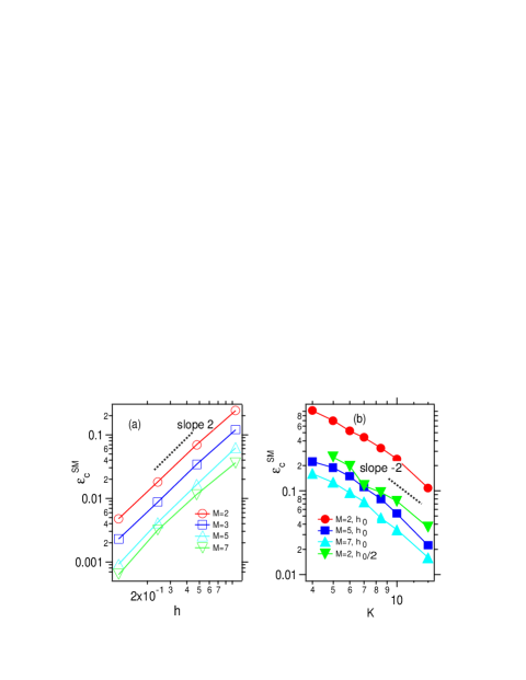
Figure 4: (Color online) (a)The critical perturbation strength $\epsilon_{c}^{SM}$ as a function of $\hbar$ for the polychromatically perturbed SM ($M=2,3,5$) with $K=3.1$. (b)The critical perturbation strength $\epsilon_{c}^{SM}$ as a function of $K$ for the polychromatically perturbed SM ($M=2,5,7$) with $\hbar=2\pi 311/2^{13}$, and $M=2$, $\hbar=2\pi 311/2^{14}$. $\epsilon_{c}^{SM}\propto\hbar^{-2}$ and $\epsilon_{c}^{SM}\propto K^{2}$ are shown by black broken lines in the panel (a) and (b), respectively. Note that the axes are in the logarithmic scale.

IV.2.2 The AM

In the case of AM, the critical value $\epsilon_{c}^{AM}$ depends upon $W$ as shown by Fig.5(a) for various values of $M$. The dependence of $\epsilon_{c}^{AM}$ upon $W$ changes at $W=W^{*}$, which is consistent with the prediction of the SCT given by Eq.(37). In particular in the regime $W>W^{*}$ it is evident that the numerical result follows the result of SCT

$$\epsilon_{c}^{AM}\sim\frac{1}{W}~{}~{}~{}~{}(W>W^{*})$$ (39)

On the contrary, in the opposite regime $W<W^{*}$ the numerical results strongly suggest that

$$\epsilon_{c}^{AM}\simeq const~{}~{}~{}(W<W^{*})$$ (40)

which do not agree with the prediction of the SCT. Such a tendency persists as $W$ decreases further, and it seems that $\epsilon_{c}^{AM}$ approaches toward a constant depending upon $M$ as $W\to 0$.

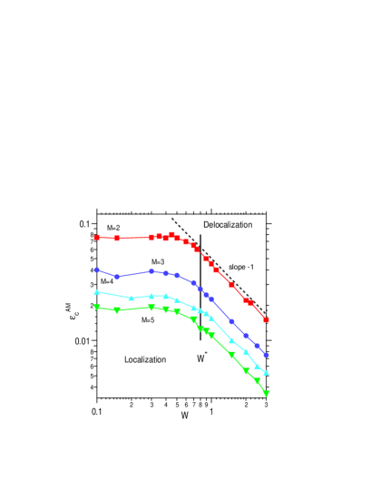
Figure 5: (Color online) The critical perturbation strength $\epsilon_{c}^{AM}$ as a function of $W$ for the polychromatically perturbed AM ($M=2,3,4,5$). $\epsilon_{c}^{AM}\propto W^{-1}$ and $W=W^{*}$ are shown in by dotted black and thick black lines, respectively. Note that the axes are in the logarithmic scale.

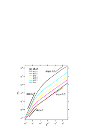
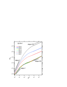
Figure 6: (Color online) The double-logarithmic plots of $m_{2}(t)$ exhibiting the critical subdiffusion at $\epsilon_{c}^{AM}$ are shown for (a)$M=2$ and (b)$M=4$. Various values of $W$ in the regimes $W<W^{*}$ and $W>W^{*}$ are examined. In the regime $W>W^{*}$ all the curves overlap. But, as $W\to 0$, $\epsilon_{c}^{AM}$ takes the same value and the ballistic transient motion of slope $2$ become more evident. One can see that in the opposite case $W\gg W^{*}$ the normal diffusion of slope $1$ first emerges before the subdiffusion sets in.

IV.2.3 More about AM: the ballistic transient

The reason why the prediction of SCT fails for the AM is tightly connected with a peculiar characteristic of the dynamics in the weak $W$ limit of AM. The basic hypothesis used for deriving Eq.(40) is the the motion of the main mode transiently exhibits the fully normal diffusion and the harmonic mode follow the same transient diffusion process. This hypothesis is not, however, correct in the weak limit of $W$, because a ballistic motion dominate the transient behavior until the scattering occurs at the mean free path length $\ell_{0}$ and makes the motion stochastic. Indeed, in Fig.6 we can show explicitly how the critical subdiffusion emerges after the ballistic transient behavior.

Let us consider the motion of the harmonic mode when the main mode visits lattice site in a ballistic way until the scattering at the mean free path $\ell_{0}$ happens. The position of the harmonic mode occurs as

$$\hat{y}_{j}(t) = \sum_{s<t}G_{j}(s)$$ (41)

$$= \sum_{s<t}\left(\sum_{n}\frac{\epsilon W}{\sqrt{M}}v_{n}|n\rangle\langle n|\right)\sin\omega_{j}s.$$

This equation tells that the particle moving at the velocity $V_{B}$ among the lattice sites $|n\rangle$ causes a randomly switching source proportional to $Wv_{n}$, which leads to diffusion of the $j$ oscillator. Then the diffusive motion is expressed by the MSD

$$\langle(\hat{y}_{j}(t)-\hat{y}_{j}(0))^{2}\rangle=\frac{\epsilon^{2}W^{2}}{M}V_{B}t,$$ (42)

and so the diffusion constant $D^{(0)}_{j}=\frac{\epsilon^{2}W^{2}}{M}V_{B}$. This motion, however, terminates the main-mode reaches $\ell_{0}$ at the time $t_{0}=\ell_{0}/V_{B}$, and $\ell_{j}$ should be

$$\ell_{j}=\sqrt{D^{(0)}_{j}t_{0}}=\frac{\epsilon\sqrt{W^{2}\ell_{0}}}{\sqrt{M}}.$$ (43)

It is independent of $W$, since $\ell_{0}\sim W^{-2}$. Substituting Eq.(43) into Eq.(34), the critical perturbation strength does no longer depends upon $W$, which is consistent with the numerical computation. In the case of SM, we considered an ideal regime such that the diffusion process in the classical limit is observed without the coherent dynamical process corresponding to the ballistic motion of AM. However, even in the case of SM, if the coherent motion is significant in the classical chaotic diffusion, we need a modification presented above.

IV.3 $M-$dependence of the critical value $\epsilon_{c}$

In the previous subsection the SCT works well for predicting the characteristics of the critical coupling strength $\epsilon_{c}$ except for the $M$-dependence. However, as is seen in Figs.4 and 5, $\epsilon_{c}$ definitely decreases with increase in $M$, and contradict with the prediction of the SCT.

With other control parameters such as $K$, $\hbar$ for SM and $W$ for AM being fixed, all the numerical results are well fitted by the empirical rule for both SM and AM:

$$\epsilon_{c}\propto\frac{1}{(M-1)}$$ (44)

as is demonstrated in Fig.7. Note that divergence at $M=1$ agrees with the absence of LDT in monochromatically perturbed SM and AM. (The log-log plot of $\epsilon_{c}$ vs $M$ does not form fine straight curves like those displayed in Fig.7.) The approach of $\epsilon$ to zero for $M\to\infty$ means that the localization is destroyed to turn into a normal diffusion by the noise with an arbitrary small amplitude.

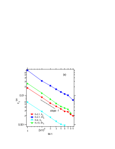
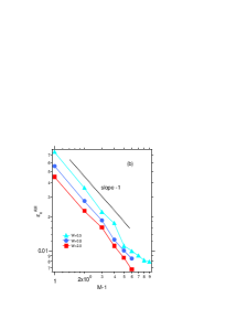
Figure 7: (Color online) (a)The critical perturbation strength $\epsilon_{c}^{SM}$ as a function of $(M-1)$ for the perturbed SM with $K=3.1$ and $K=5$, $\hbar=\hbar_{0}$. (b)The critical perturbation strength $\epsilon_{c}^{AM}$ as a function of $(M-1)$ for the perturbed AM with $W=0.5,0.8,2.0$. Note that the axes are in the logarithmic scale. The line with slope $-1$ is shown as a reference.

Having the rule of Eq.(44) in mind, we reorganize our numerical results by plotting $(M-1)\epsilon_{c}$ vs other parameters. We replot the data in Fig.4(a) and (b) by assigning the vertical axis to $\epsilon_{c}(M-1)$ and the horizontal axis to $K/\hbar$. All the data points are on a unified single master curve, which implies the rule

$$\epsilon^{SM}_{c}\propto\frac{K^{2}}{\hbar^{2}(M-1)}$$ (45)

exits. A slight discrepancy exits between upper side data and the lower side data. Its origin will be the fact that the data of the upper side belongs to smaller $K$ regime for which significant deviation from the relation $\ell_{0}\propto K^{2}/\hbar^{2}$ occurs. (See caption of the Fig.8.)

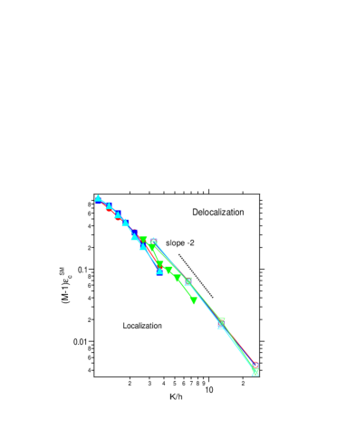
Figure 8: (Color online) The phase diagrams and the critical values $(M-1)\epsilon_{C}^{SM}$ in the plane $((M-1)\epsilon,~{}K/\hbar)$ for the SM. Data with various values of $M$, $K$ and $\hbar$ are plotted. The data plotted by empty circles, squares and crosses, which are on a common line in the lower side, are the data in Fig.4(a). They have the same $K=3.1$, which is not $K\gg 1$, and so the common line slightly shifts from the curves of other data. The line with slope $-2$ is shown as a reference.

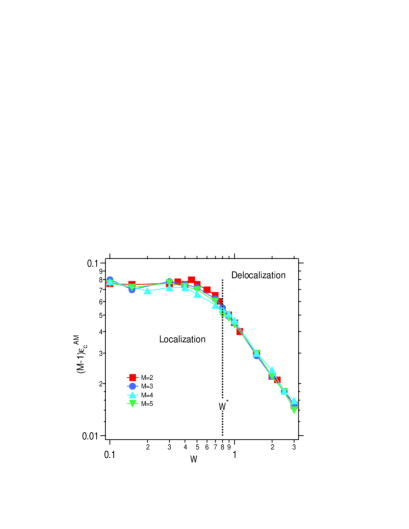
Figure 9: (Color online) The phase diagrams in a plane $((M-1)\epsilon,W)$ for the polychromatically perturbed AM ($M=2,3,4,5$). $W=W^{*}$ is shown by dotted black line. Note that the axes are in the real scale.

The same plot for the AM on the $((M-1)\epsilon,W)$ plane is shown in Fig.9, which manifests that almost all the data are on a single master curve irrespective of $W<W^{*}$ or $W>W^{*}$, which implies the rule

$$\epsilon_{c}^{AM}\propto\begin{cases}\dfrac{1}{M-1}~{}~{}~{}~{}~{}~{}~{}(W<W^{*}),\\ \dfrac{1}{W(M-1)}~{}~{}~{}(W>W^{*}).\end{cases}$$ (46)

The behavior of the subdiffusion index $\alpha=2/(M+1)$, which can not be explained by SCT of the localization, seems to be coordinate with the approach of $\epsilon_{c}$ to $0$ with increasing $M$. The SCT overestimates $\epsilon_{c}$. Indeed, the second term in the r.h.s. of Eq.(25), which evaluates the reduction of the diffusion constant from the ideal diffusion rate by the backscattering effect, seems to overestimated. Roughly speaking, this integral yields the surface area $S_{M+1}\sim{M}^{-M/2}$, which cancels with the normalization factor $1/\sqrt{M}$ and takes off the $M$-dependence from $\epsilon_{c}$. If the surface factor is replaced by a further smaller one

$$S_{M}^{\prime}=\frac{1}{M!}S_{M},$$ (47)

the SCT succeeds in predicting all the characteristics of the critical coupling strength. This replacement means that the $M$-harmonic degrees of freedom is indistinguishable, but we could not explain the origin of the above reduction.

V Summary and discussion

We investigated the localization-delocalization transition (LDT) of the SM (standard map) and the AM (Anderson map) which are dynamically perturbed by polychromatically periodic oscillations for the initially localized quantum wavepacket.

In the SM and AM, for number of colors $M$ more than two, the LDT always takes place with increase in the perturbation strength $\epsilon$, and the critical exponents at the critical point decrease with $M$. In particular, the critical diffusion exponent decreases as $\alpha\simeq 2/(M+1)$ in accordance with the prediction of one-parameter scaling theory (OPST).

In the present paper, we paid particular attentions to the dependence of the critical perturbation strength $\epsilon_{c}$ upon the control parameters. If the number of color $M$ is fixed, the control parameter dependencies are well predicted by the self-consistent theory (SCT) of the localization for both SM and AM if basic hypothesis are properly modified. On the other hand, the SCT predicts that $\epsilon_{c}$ does not depends on $M$, while numerical results reveal that $\epsilon_{c}$ reduces drastically as $\epsilon_{c}\propto 1/(M-1)$ with an increase of $M$.

The LDT leading to the normal diffusion is a decoherence transition, which is basically originated by the entanglement among wavefunctions spanning the $(M+1)-$dimensional Hilbert space. Such an entanglement induces the drastic decrease of $\alpha$ and $\epsilon_{c}$ with increase of $M$. If $M+1$ can be identified with the spatial dimension $d$, as is suggested by the Maryland transform, then can we expect such a steep dependence of critical properties on $d$ for Anderson transition in $d$-dimensional disordered lattice? This is a quite interesting question footnote-epsc .

Owing to such a decrease of threshold $\epsilon_{c}$, the polychromic perturbation is identified with a white noise in the limit $M\to\infty$, and it can destroy the localization at an arbitrary small amplitude.

It is also a quite interesting problem how such characteristic critical behaviors are observed for the dynamical delocalization of the time-continuous system yamada99 , which shares much common nature with the present AM in the limit $W\to 0$. In particular, whether the limiting behavior $\epsilon_{c}\to$ const. in the regime of $W\ll 1$ is intrinsic and is not due to the discreteness of time evolution is an important problem yamada20 .

Appendix A Malyland transform and tight-binding representation

We consider an eigenvalue equation

$$\hat{U}_{aut}|u\rangle={\rm e}^{-i\gamma}|u\rangle$$ (48)

for the time-evolution operator of the Hamiltonian (7),

$$\hat{U}_{aut}={\rm e}^{-i\hat{A}}{\rm e}^{-i\hat{B}}{\rm e}^{-i\hat{C}},$$ (49)

where $\gamma$ and $|u\rangle$ are the quasi-eigenvalue and quasi-eigenstate.

For the SM,

$$\begin{cases}{\rm e}^{-i\hat{A}}={\rm e}^{-\frac{i}{\hbar}[T(\hat{p})+\sum_{j}^{M}\omega_{j}\hat{J}_{j}]},\\ {\rm e}^{-i\hat{B}}={\rm e}^{-\frac{i}{\hbar}\epsilon\hat{V}(q)\frac{\epsilon}{\sqrt{M}}\sum_{j}^{M}\cos\phi_{j}},\\ {\rm e}^{-i\hat{C}}={\rm e}^{-\frac{i}{\hbar}V(\hat{q})}.\end{cases}$$ (50)

The eigenvalue equation we take the representation using eigenstate $|m\rangle(m\in{\mathbb{Z}})$ of momentum $\hat{p}$ and the action eigenstate $\{|m_{1}\rangle,...,|m_{M}\rangle\}(m_{i}\in{\mathbb{Z}})$ of the $M$ number of $J$-oscillators as $u(m,m_{1},...,m_{M})=(\langle m|\otimes\langle m_{1},...,m_{M}|)|u\rangle$. Then by applying the Maryland transform, the eigenvalue equation can be mapped into the following $(M+1)$-dimensional tight-binding system with aperiodic and singular on-site potential:

$$\tan\left[\frac{\hbar^{2}m^{2}/2+\hbar\sum_{j}^{M}m_{j}\omega_{j}}{2\hbar}-\frac{\gamma}{2}\right]u(m,m_{1},...,m_{M})+$$

$$\sum_{m^{\prime},m_{1}^{\prime},...,m_{M}^{\prime}}\langle m,m_{1},...,m_{M}|\hat{t}_{SM}|m^{\prime},m_{1}^{\prime},...,m_{M}^{\prime}\rangle u(m^{\prime},m_{1}^{\prime},...,m_{M}^{\prime})=0,$$ (51)

where the transfer matrix element is

$$\langle m,m_{1},...,m_{M}|\hat{t}_{SM}|m^{\prime},m_{1}^{{}^{\prime}},...,m_{M}^{{}^{\prime}}\rangle$$ (52)

$$= \frac{1}{(2\pi)^{M+1}}\int_{0}^{2\pi}...\int_{0}^{2\pi}dqd\phi_{1}...d\phi_{M}{\rm e}^{-i(m-m^{\prime})q}{\rm e}^{i\sum_{j}^{M}(m_{j}-m_{j}^{\prime})\phi_{j}}\tan\left[\frac{K\cos q(1+\frac{\epsilon}{\sqrt{M}}\sum_{j}^{M}\cos\phi_{j})}{2\hbar}\right].$$

On the other hand, for the polychromatically perturbed AM, using

$$\begin{cases}{\rm e}^{-i\hat{A}}={\rm e}^{-\frac{i}{\hbar}(Wv(\hat{q})+\sum_{j}^{M}\omega_{i}\hat{J}_{j})},\\ {\rm e}^{-i\hat{B}}={\rm e}^{-\frac{i}{\hbar}v(\hat{q})\frac{\epsilon W}{\sqrt{M}}\sum_{j}^{M}\cos\phi_{j}},\\ {\rm e}^{-i\hat{C}}={\rm e}^{-\frac{i}{\hbar}2\cos(\hat{p}/\hbar)}\end{cases}$$ (53)

we can also obtain the following $(M+1)-$dimensional tight-binding expression:

$$\tan\left[\frac{Wv_{n}+\hbar\sum_{j}^{M}m_{j}\omega_{j}}{2\hbar}-\frac{\gamma}{2}\right]u(n,m_{1},...,m_{M})+$$

$$\sum_{n^{\prime},m_{1}^{\prime},...,m_{M}^{\prime}}\langle n,m_{1},...,m_{M}|\hat{t}_{AM}|n^{\prime},m_{1}^{\prime},...,m_{M}^{\prime}\rangle u(n^{\prime},m_{1}^{\prime},...,m_{M}^{\prime})=0,$$ (54)

where the transfer matrix element is

$$\langle n,m_{1},...,m_{M}|\hat{t}_{AM}|n^{\prime},m_{1}^{{}^{\prime}},...,m_{M}^{{}^{\prime}}\rangle$$ (55)

$$= \Braket{n,m_{1},...,m_{M}}{i\frac{e^{-i\frac{\epsilon W}{\sqrt{M}}v_{n}(\sum_{i}^{M}\cos\phi_{i})/\hbar}-e^{i2\cos(\hat{p}/\hbar)/\hbar}}{e^{-i\frac{\epsilon W}{\sqrt{M}}v_{n}(\sum_{i}^{M}\cos\phi_{i})/\hbar}+e^{i2\cos(\hat{p}/\hbar)/\hbar}}}{n^{\prime},m_{1}^{{}^{\prime}},...,m_{M}^{{}^{\prime}}}.$$

The $n$ denotes one-dimensional disorder site of the AM. In this representation, the effect of the disorder strength $W$ of the diagonal term saturates at $W^{*}(=2\pi\hbar)$ and increasing beyond $W^{*}$ does not affect the diagonal disorder. Also, it can be seen that the effect of the perturbation is embedded in the off-diagonal term representing hopping in the form of $\epsilon W$ for $W>W^{*}$. For this reason, the critical perturbation strength indicates the $W-$dependence in Eq.(39) when $W>W^{*}$.

It follows that the $(M+1)-$dimensional tight-binding models of the SM and AM have singularity of the on-site energy caused by tangent function and long-range hopping caused by kick. However, in the case of $\epsilon\neq 0$, the evaluation of matrix elements is not easy since the stochastic quantity $v_{n}$ is contained in addition to both operators $\hat{q}$ and $\hat{p}$.

Appendix B One-parameter scaling theory and diffusion exponent

In the long-time limit ($t\to\infty$), we can predict asymptotic behavior of MSD as

$$m_{2}(t)\sim\begin{cases}\xi^{2}&(\epsilon<\epsilon_{c})\\ Dt&(\epsilon>\epsilon_{c}),\end{cases}$$ (56)

for the localized ($\epsilon<\epsilon_{c}$) and delocalized regime ($\epsilon>\epsilon_{c}$), respectively. Here $D$ and $\xi$ denote the diffusion coefficient and localization length, respectively. In the vicinity of LDT $\epsilon\simeq\epsilon_{c}$, with two critical exponents $\nu$ and $s$, we assume

$$\begin{cases}D\sim(\epsilon-\epsilon_{c})^{s}&(\epsilon>\epsilon_{c})\\ \xi\sim(\epsilon_{c}-\epsilon)^{-\nu}&(\epsilon<\epsilon_{c},).\end{cases}$$ (57)

The exponents satisfy Wegner relation

$$s=(d-2)\nu$$ (58)

where $d$ is spatial dimension wegner76 .

We can use the following scaling hypothesis

$$m_{2}(t)=a^{2}F_{1}(L_{t}/a,\xi/a),$$ (59)

with two-variable scaling function $F_{1}(x_{1},x_{2})$. Here an unique characteristic length $L_{t}$ associated with dynamics as

$$L_{t}\sim t^{\sigma},$$ (60)

where $\sigma$ is a dynamical exponent. If we set $a=\xi$, then $m_{2}$ scales like

$$m_{2}(t) = \xi^{2}F_{1}(t^{\sigma}/\xi,1),$$ (61)

$$= t^{2\sigma}F_{2}(t^{\sigma/\nu}(\epsilon-\epsilon_{c})),$$ (62)

where $F_{2}(x)$ is a one-variable scaling function. A relation

$$2\sigma+\frac{\sigma s}{\nu}=1,$$ (63)

must be satisfied to recover the condition (57). Using Wegner relation it follows

$$\sigma=\frac{1}{d}.$$ (64)

Therefore, at the critical point $\epsilon=\epsilon_{c}$ of LDT, the MSD shows subdiffusion

$$m_{2}(t)\sim t^{\alpha}.$$ (65)

with the diffusion exponent

$$\alpha=\frac{2}{d}=\frac{2}{M+1}.$$ (66)

Appendix C Critical localization exponents of LDT in the polychromatically perturbed quantum maps

In this appendix, the finite-time scaling analysis of the LDT by using MSD $m_{2}(t)$ and the $M-$dependence of the critical exponent in the perturbed SM and AM are shown. However, note that pursuing $\nu$ by numerical calculations with high accuracy is not the purpose of this paper.

First, let us consider the following quantity

$$\Lambda_{s}(\epsilon,t)=\frac{\Lambda(\epsilon,t)}{\Lambda(\epsilon_{c},t)}-1$$ (67)

as a scaling variable. For $\epsilon>\epsilon_{c}$, the $\Lambda_{s}$ increases and the wave packet delocalizes with time. On the contrary, for $\epsilon<\epsilon_{c}$, $\Lambda_{s}$ decreases with time and the wavepacket turns to the localization. Around the LDT point of the perturbed cases by $M$ modes, the localization length $\xi$ is supposed to diverge

$$\xi\sim|\epsilon_{c}-\epsilon|^{-\nu}$$ (68)

as $\epsilon\to\epsilon_{c}$ for the localized regime $\epsilon\leq\epsilon_{c}$. $\nu$ of LDT is the critical localization exponent characterizing divergence of the localization length and depends on the number of modes $M$, but after that, the subscript $M$ is abbreviated for simplicity of the notation.

For $\Lambda_{s}(t)$, it is assumed that in the vicinity of this LDT one-parameter scaling theory (OPST) is established as the parameter is the localization length $\xi(\epsilon)$. Then, $\Lambda_{s}(t)$ can be expressed as,

$$\Lambda_{s}(\epsilon,t) = F(x),$$ (69)

where

$$x=(\epsilon_{c}-\epsilon)t^{\alpha/2\nu}.$$ (70)

$F(x)$ is a differentiable scaling function and $\alpha$ is the diffusion index. Therefore, $F(x)$ is expand around the critical point as follows:

$$F(x)=F(0)+C_{1}(t)(\epsilon_{c}-\epsilon)+C_{2}(t)(\epsilon_{c}-\epsilon)^{2}+....$$ (71)

, and

$$C_{1}(t)\propto t^{\alpha/2\nu}.$$ (72)

As a result, the critical exponent $\nu$ of LDT can be determined using data obtained by numerical calculation and the above relation. If we use the $\nu$ and $\alpha$, we can ride $\Lambda_{s}$ for various $\epsilon$ on a smooth function by shifting the time axis to $x$. This is consistent with formation of the scaling hypothesis.

Figure 10 shows the scaling curve constructed by the time-dependent data at various $\epsilon$ near $\epsilon_{c}$ in SM of $M=3$ with $K=3.1$, $\hbar=\hbar_{0}$. Figure 10(b) is a plot of $\Lambda_{s}(\epsilon,t)$ as a function of $\epsilon$ at several times $t$, and this crosses at the critical point $\epsilon_{c}$. Also, Fig. 10(c) shows $C_{1}(t)$ as a function of $t$, and the critical exponent $\nu$ is determined by best fitting the slope, and the scaling curve $F(x)$ is displayed in 10(a) using the critical values. It is well scaled and demonstrates the validity of OPST. Further, Fig.11 displays the result of the finite-time scaling analysis for polychromatically perturbed SM ($M=7$) with $K=3.1$ and $\hbar=\hbar_{0}$. For any number of colors $M$, the LDT is well scaled against perturbation strength changes, suggesting that LDT can be described fairly well within the OPST framework.

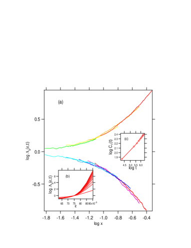
Figure 10: (Color online) The results of the critical scaling analysis for trichromatically perturbed SM ($M=3$) with $K=3.1$ and $\hbar=\hbar_{0}$. (a)The scaled variable $\Lambda_{s}(\epsilon,t)$ as a function of $x=|\epsilon_{c}^{SM}-\epsilon|t^{\alpha/2\nu}$ for some values of $\epsilon$. (b)The scaled MSD $\Lambda_{s}(\epsilon,t)$ with $\alpha\simeq 0.46$ as a function of $\epsilon$ for some pick up times. The crossing point is $\epsilon_{c}^{SM}\simeq 0.13$. (c)$C_{1}(t)$ as a function of $t$. The critical exponent $\nu\simeq 0.95$ is determined by a scaling relation Eq.(72) by the least-square fit.

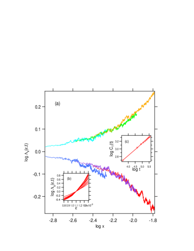
Figure 11: (Color online) The results of the critical scaling analysis for polychromatically perturbed SM ($M=7$) with $K=3.1$ and $\hbar=\hbar_{0}$. (a)The scaled variable $\Lambda_{s}(\epsilon,t)$ as a function of $x=|\epsilon_{c}^{SM}-\epsilon|t^{\alpha/2\nu}$ for some values of $\epsilon$. (b)The scaled MSD $\Lambda_{s}(\epsilon,t)$ with $\alpha\simeq 0.25$ as a function of $\epsilon$ for some pick up time $t_{m}$. The crossing point is $\epsilon_{c}^{SM}\simeq 0.018$. (c)$C_{1}(t)$ as a function of $t$. The critical exponent $\nu\simeq 0.35$ is determined by a scaling relation Eq.(72) by the least-square fit.

In Fig.12, we show result of finite-time scaling analysis for AM of $M=2$ with $W=2.0(>W^{*})$. The method used here is the same as that used in the paper [2] for AM of $M=5$ with $W=0.5(<W^{*})$. We choose the following quantity as a scaling variable

$$\Lambda_{s}(\epsilon,t)=\log\Lambda(\epsilon,t).$$ (73)

Figure 12(b) shows a plot of $\Lambda_{s}(t)$ as a function of $\epsilon$ at several times $t$, and it can be seen that this intersects at the critical point $\epsilon_{c}$. In addition, Fig.12(c) shows a plot of

$$s(t)=\frac{\Lambda_{s}(\epsilon,t)-\Lambda_{s}(\epsilon_{c},t)}{|\epsilon_{c}-\epsilon|}\propto t^{\alpha/2\nu}$$ (74)

as a function of $t$, and the critical localization exponent $\nu$ is determined by best fitting this slope. In Fig.12(a), we plot $\Lambda_{s}$ as a function of $x$ for different values of $\epsilon$ by using the obtained the critical exponent $\nu$. Similar results to case in the paper [2] is obtained.

Further, Fig.13 and 14 displays the results of the finite-time critical scaling analysis for trichromatically perturbed AM of $M=3$ with $W=0.5(<W^{*})$ and AM ($M=7$) with $W=2.0(>W^{*})$, respectively. As a result, even in the AM, the OPST is well established for the LDT regardless of the number of colors $M$ and the disorder strength $W$. The localization critical exponent $\nu$ obtained is almost similar if $M$ is the same. The result strongly suggests that the LDT is a universal transition phenomenon.

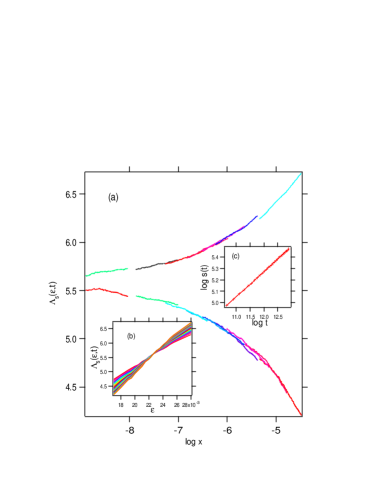
Figure 12: (Color online) The results of the critical scaling analysis for dichromatically perturbed AM ($M=2$) with $W=2.0$($>W^{*}$). (a)The same scaled MSD $\Lambda_{s}(\epsilon,t)$ as a function of $x=\xi_{0}|\epsilon_{c}^{AM}-\epsilon|^{-\nu}t^{\alpha/2\nu}$ for some values of $\epsilon$, where $\xi_{0}$ is the localization length in the unperturbed case. (b)The scaled $\Lambda_{s}(\epsilon,t)$ with $\alpha=0.65$ as a function of $\epsilon$ for some pick up times. The crossing point is $\epsilon_{c}^{AM}\simeq 0.0225$. (c)$s(t)$ as a function of $t$. The critical exponent $\nu\simeq 1.48$ is determined by a scaling relation Eq.(74) by the least-square fit.

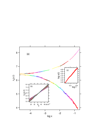
Figure 13: (Color online) The results of the critical scaling analysis for trichromatically perturbed AM ($M=3$) with $W=0.5(<W^{*})$. (a)The same scaled MSD $\Lambda_{s}(\epsilon,t)$ as a function of $x=\xi_{0}|\epsilon_{c}^{AM}-\epsilon|^{-\nu}t^{\alpha/2\nu}$ for some values of $\epsilon$, where $\xi_{0}$ is the localization length in the unperturbed case. (b)The scaled MSD $\Lambda_{s}(\epsilon,t)$ with $\alpha=0.51$ as a function of $\epsilon$ for some pick up times. The crossing point is $\epsilon_{c}^{AM}\simeq 0.036$. (c)$s(t)$ as a function of $t$. The critical exponent $\nu\simeq 1.18$ is determined least-square fit of (b).

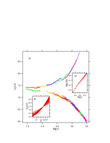
Figure 14: (Color online) The results of the critical scaling analysis for polychromatically perturbed AM ($M=7$) with $W=2.0(>W^{*})$. (a)The same scaled MSD $\Lambda_{s}(\epsilon,t)$ as a function of $x=\xi_{0}|\epsilon_{c}^{AM}-\epsilon|^{-\nu}t^{\alpha/2\nu}$ for some values of $\epsilon$, where $\xi_{0}$ is the localization length in the unperturbed case. (b)The scaled MSD $\Lambda_{s}(\epsilon,t)$ with $\alpha=0.25$ as a function of $\epsilon$ for some pick up times. The crossing point is $\epsilon_{c}^{AM}\simeq 0.0034$. (c)$s(t)$ as a function of $t$. The critical exponent $\nu\simeq 0.49$ is determined least-square fit of (b).

For $M=2$ to $M=7$, in LDT of SM and AM, the critical exponents $\nu$ obtained from the critical scaling analysis are arranged in table 1. The results of the critical exponent of the $d-$dimensional Anderson transition are also cited from various literatures. It can be seen that in the perturbed SM and AM with $M$ color modes the critical localization exponent of LDT tend to be similar to the Anderson transition of the $d(=M+1)-$dimensional random system. In other words, the critical exponent $\nu$ of LDT decreases with $M\to\infty$. In the case of the $d-$dimensional Anderson transition, at least in $d\to\infty$, the mean field approximation is in exact, and it is considered asymptotic to the result of SCT $\nu=1/2$. This can also be imagined from the fact that in the Anderson transition, spatial connections are important in higher dimensions and the quantum interference effect fades. However, in LDT in SM and AM, the exponent tend to decrease to a value smaller than $\nu=1/2$ predicted by SCT as $M$ increases. Note that in these cases, Harris’ inequality $\nu\geq\frac{2}{d}$ is not broken harris74 .

	M=2	M=3	M=4	M=5	M=6	M=7
SM($K=3.1,\hbar=0.24$)	1.37	0.95	0.70	0.50	0.50	0.40
Ref.chabe08	1.58	1.15	–	–	–	–
Ref.borgonovi97	1.537	1.017	–	–	–	–
AM(W=0.5)	1.46	1.18	0.80	0.62	0.53	0.41
AM(W=2.0)	1.48	1.01	0.88	0.65	0.57	0.49
	d=3	d=4	d=5	d=6	d=7	d=8
Ref.markos06	1.57	1.12	0.93	–	–	–
Ref.garcia07	1.52	1.03	0.84	0.78	–	–
Ref.slevin14	1.57	1.15	0.97	–	–	–
Ref.tarquini17	1.57	1.11	0.96	0.84	–	–

Table 1: The critical exponents numerically obtained by the scaling analysis which characterizes the critical dynamics in the polychromatically perturbed SM and AM for $M=2\sim 7$. Ref.chabe08 and Ref.borgonovi97 are results has already been reported for SM. The lower four lines show the critical exponents numerically obtained for the $d-$dimensional disordered systems markos06 ; garcia07 ; slevin14 ; tarquini17 .

References

- (1) P. W. Anderson, Phys. Rev. 109, 1492-1505 (1958).
- (2) K.Ishii, Prog. Theor. Phys. Suppl. 53, 77(1973).
- (3) H.S. Yamada, F. Matsui and K.S. Ikeda, Phys. Rev. E 92, 062908(2015).
- (4) H.S. Yamada, F. Matsui and K.S. Ikeda, Phys. Rev. E 97, 012210(2018).
- (5) G. Casati, B. V. Chirikov,F. M. Izraelev, J.Ford, Stochastic behavior of a quantum pendulum under a periodic perturbation (Springer-Verlag,Berlin,1979) ed. by G.Casati and J.Ford .pp334.
- (6) G.Casati, I.Guarneri and D.L.Shepelyansky, Phys. Rev. Lett. 62, 345(1989).
- (7) F.Borgonovi and D.L.Shepelyansky, Physica D109, 24 (1997).
- (8) J.Chabe, G.Lemarie, B.Gremaud, D.Delande, and P.Szriftgiser, Phys. Rev. Lett. 101, 255702(2008).
- (9) J. Wang and A. M. Garcia-Garcia, Phys. Rev. E 79, 036206(2009).
- (10) G. Lemarie, H.Lignier, D.Delande, P.Szriftgiser, and J.-C.Garreau, Phys. Rev. Lett. 105, 090601(2010).
- (11) C. Tian, A. Altland, and M. Garst, Phys. Rev. Lett. 107, 074101(2011).
- (12) M.Lopez, J.F.Clement, P.Szriftgiser, J.C.Garreau, and D.Delande, Phys. Rev. Lett. 108, 095701(2012).
- (13) M. Lopez, J.-F. Clement, G. Lemarie, D. Delande, P. Szriftgiser, and J. C. Garreau, New J. Phys. 15, 065013(2013).
- (14) I. Manai et al., Phys. Rev. Lett. 115, 240603(2015).
- (15) H.Yamada and K. Ikeda, Phys. Lett. A 248, 179-184(1998).
- (16) H.S. Yamada and K.S. Ikeda, Phys. Rev. E 59, 5214(1999).
- (17) H. Yamada and K. S. Ikeda, Phys. Lett. A 328, 170 (2004).
- (18) P. Wolfle and D. Vollhardt, Int. J. Mod. Phys B 24, 1526(2010).
- (19) H.S.Yamada and K.S.Ikeda, Phys. Rev. E 82, 060102(R)(2010); Eur. Phys. J. B 85, 41(2012); Eur. Phys. J. B 85, 195(2012).
- (20) S. Fishman, D.R.Grempel, R.E.Prange, Phys. Rev. Lett. 49, 509 (1982); D.R. Grempel, R.E. Prange and S. Fishman, Phys. Rev. A 29, 1639(1984); R.E. Prange, D.R. Grempel, and S. Fishman, Phys. Rev. B 29, 6500-6512(1984).
- (21) G. Casati, B.V. Chirikov, and D.L. Shepelyansky, Phys. Rev. Lett. 53. 2525 (1984).
- (22) L.M.Lifshiz, S.A.Gredeskul and L.A.Pastur, Introduction to the theory of Disordered Systems, (Wiley, New York,1988).
- (23) Delande et al. selected for SCT and showed the dependent result of . For , as shown in lopez13 , and in a limit , .
- (24) P. Markos, Acta Phys. Slovaca 56, 561(2006).
- (25) Antonio M. Garca-Garcia and Emilio Cuevas, Phys. Rev. B 75,174203(2007).
- (26) Yoshiki Ueoka, and Keith Slevin, J. Phys. Soc. Jpn. 83, 084711(2014).
- (27) E. Tarquini, G. Biroli, and M. Tarzia, Phys. Rev. B 95, 094204(2017).
- (28) J.Wegner, Z.Phys.B 25, 327(1976).
- (29) A.B.Harris, J.Phys.C 7, 1671-1692(1974). J.T.Chayes, L.Chayes, D.S.Fisher, and T.Spencer, Phys.Rev. Lett.57, 2999-3002(1986).
- (30) The value of the diffusion index in the dimensional Anderson transition is not yet known. However, it is known that in the Anderson model of the disorder strength , the dimensionality of the critical strength is for large , which corresponds to the behavior in the large-connectivity limit garcia07 ; tarquini17 .
- (31) H.S. Yamada and K.S. Ikeda, in preparation.