Weak cosmic growth in coupled dark energy with a Lagrangian formulation

Abstract

We investigate a dark energy scenario in which a canonical scalar field $\phi$ is coupled to the four velocity $u_{c}^{\mu}$ of cold dark matter (CDM) through a derivative interaction $u_{c}^{\mu}\partial_{\mu}\phi$. The coupling is described by an interacting Lagrangian $f(X,Z)$, where $f$ depends on $X=-\partial^{\mu}\phi\partial_{\mu}\phi/2$ and $Z=u_{c}^{\mu}\partial_{\mu}\phi$. We derive stability conditions of linear scalar perturbations for the wavelength deep inside the Hubble radius and show that the effective CDM sound speed is close to 0 as in the standard uncoupled case, while the scalar-field propagation speed is affected by the interacting term $f$. Under a quasi-static approximation, we also obtain a general expression of the effective gravitational coupling felt by the CDM perturbation. We study the late-time cosmological dynamics for the coupling $f\propto X^{(2-m)/2}Z^{m}$ and show that the gravitational coupling weaker than the Newton constant can be naturally realized for $m>0$ on scales relevant to the growth of large-scale structures. This allows the possibility for alleviating the tension of $\sigma_{8}$ between low- and high-redshift measurements.

I Introduction

The fundamental pillar in modern cosmology consists of two dark unknown components– dubbed dark energy (DE) and dark matter (DM). The simplest candidate for DE is the cosmological constant $\Lambda$ Peebles:1984ge , with the equation of state (EOS) corresponding to $w=-1$. The main source for DM is nonrelativistic cold dark matter (CDM) Peebles:1982ff with the EOS satisfying $|w|\ll 1$ to explain the observed galaxy clusterings. The $\Lambda$CDM model is regarded as the standard cosmological paradigm, but it is difficult to reconcile the observed energy scale of $\Lambda$ with the vacuum energy associated with particle physics Weinberg . Moreover, the tension of today’s Hubble constant $H_{0}$ between low- and high-redshift measurements has been serious in the $\Lambda$CDM model Riess:2016jrr ; Aghanim:2018eyx ; Verde:2019ivm ; Riess:2019cxk ; Freedman:2019jwv ; Wong:2019kwg ; Reid:2019tiq ; Shajib:2019toy . A similar tension is also present for the amplitude of matter density contrast $\sigma_{8}$ Macaulay:2013swa ; Nesseris:2017vor ; Hildebrandt:2016iqg ; Joudaki:2017zdt within the sphere of radius $8\,h^{-1}$ Mpc, where $H_{0}=100\,h$ km s^-1 Mpc^-1.

The recent studies have shown that the presence of an interaction between DE and DM can alleviate the aforementioned tensions of $H_{0}$ and/or $\sigma_{8}$ Wands ; Kumar:2016zpg ; Kumar:2017dnp ; DiValentino:2017iww ; An:2017crg ; Kaza ; Yang:2018euj ; Pan:2019gop ; DiValentino:2019ffd ; Yang:2019uog . In most of these works, phenomenological interacting terms like $\pm\xi H\rho_{\rm DE}$ are added to the CDM and DE continuity equations at the background level, where $\xi$ is a coupling constant, $H$ is the Hubble expansion rate, and $\rho_{\rm DE}$ is the DE density (see Refs. Dalal:2001dt ; Zimdahl:2001ar ; Chimento:2003iea ; Wang1 ; Wei:2006ut ; Amendola:2006dg ; Guo:2007zk ; Gavela:2009cy ; Jackson:2009mz ; Faraoni:2014vra for earlier works). In this approach, there is no satisfactory prescription for promoting the phenomenological background equations to their fully covariant forms. In other words, the two covariant theories which give rise to the same background equations can lead to different dynamics of cosmological perturbations. This pauses a problem of how to define the perturbed quantities properly Tamanini:2015iia , which is related to unphysical instabilities of perturbations reported in Refs. Valiviita:2008iv ; Valiviita:2009nu .

On the other hand, the Lagrangian formulation of coupled DE and DM is not plagued by this problem in that the interacting terms are uniquely fixed both at the levels of background and perturbations. In this vein, the theories of coupled DE and DM were constructed in Refs. Pourtsidou:2013nha ; Boehmer:2015kta ; Boehmer:2015sha ; Skordis:2015yra ; Koivisto:2015qua ; Pourtsidou:2016ico ; Dutta:2017kch ; Kase:2019veo by using a so-called Schutz-Sorkin action Sorkin ; Brown in the DM sector (see also Refs. Bettoni:2011fs ; Bettoni:2015wla for nonminimally coupled DM). The perfect fluid of CDM can be described by the Schutz-Sorkin action containing physical quantities like the fluid density $\rho_{c}$ and the four velocity $u_{c}^{\mu}$ besides Lagrange multipliers. This prescription has an advantage of dealing with both scalar and vector perturbations in the fluid sector on any space-time background DGS ; DeFelice:2016yws ; Kase:2018nwt ; Frusciante:2018tvu ; Naka2019 .

If a scalar field $\phi$ is responsible for the DE sector, the first possible interacting Lagrangian is of the form ${\cal L}_{{\rm int}1}=-\sqrt{-g}f_{1}(\phi,X)\rho_{c}(n_{c})$ Boehmer:2015kta ; Barros ; Kase:2019veo , where $g$ is the determinant of metric tensor $g_{\mu\nu}$, $f_{1}$ is a function of $\phi$ and $X=-\partial^{\mu}\phi\partial_{\mu}\phi/2$, and $\rho_{c}$ depends on the CDM number density $n_{c}$. The $\phi$-dependent coupling $f_{1}$ arises from nonminimally coupled gravitational theories after the conformal transformation to the Einstein frame Amendola99a ; Fujii . In the Einstein frame, this theory corresponds to the coupled DE and DM scenario originally advocated in Refs. Wetterich ; Amendola99 (see also Refs. Gumjudpai ; Amendola06 ). Inclusion of $X$ dependence in $f_{1}$ leads to different dynamics of background and perturbations Barros ; Kase:2019veo .

The other possible coupling between DE and CDM is a field derivative coupling to the fluid four velocity, which is quantified by the scalar combination $Z=u_{c}^{\mu}\partial_{\mu}\phi$. The interacting Lagrangian containing the linear dependence of $Z$ in the form ${\cal L}_{{\rm int}2}=\sqrt{-g}f_{2}(n_{c},\phi)Z$ was proposed in Ref. Boehmer:2015sha . Recently, this was further extended to include the $X$ dependence in $f_{2}$ Kase:2019veo . More general coupled DE and DM theories with the nonlinear dependence of $Z$ were studied in Refs. Pourtsidou:2013nha ; Skordis:2015yra . In Ref. Pourtsidou:2016ico , it was shown that the quadratic interacting Lagrangian of the form ${\cal L}_{{\rm int}2}=\sqrt{-g}\,Z^{2}$ can lead to an interesting possibility for alleviating the problem of $\sigma_{8}$ tension by suppressing the growth of large-scale structures. This property comes from a pure momentum transfer between DE and DM. We note that all the coupling terms mentioned above are accommodated by a general interacting Lagrangian of the form ${\cal L}_{{\rm int}}=\sqrt{-g}\,f(n_{c},\phi,X,Z)$, as advocated in Ref. Pourtsidou:2013nha .

In this paper, we will study the cosmological dynamics of coupled DE and DM for the interacting Lagrangian ${\cal L}_{{\rm int}}=\sqrt{-g}\,f(X,Z)$, where $f$ is a function of $X$ and $Z$. The DE and DM sectors are described by a nonminimally coupled scalar field with a potential $V(\phi)$ and a perfect fluid with the Schutz-Sorkin action, respectively. Unlike the analysis of Refs. Boehmer:2015sha ; Koivisto:2015qua ; Kase:2019veo , our interacting theory contains the nonlinear dependence of $Z$. Moreover, it can accommodate the coupling $f(Z)=Z^{2}$ mentioned above as a special case. It is also possible to include the dependence of $\phi$ in $f$, but this does not crucially modify the dynamics of perturbations. On the other hand, inclusion of the $n_{c}$ dependence in $f$ generally gives rise to a nonvanishing CDM sound speed Koivisto:2015qua ; Kase:2019veo , so we do not take it into account to avoid causing a problem for the structure formation.

We will obtain the full linear perturbation equations of motion in a gauge-ready form and identify conditions for the absence of scalar ghosts and Laplacian instabilities. The effective gravitational couplings of CDM perturbations are also derived for general functions $f(X,Z)$ under a quasi-static approximation on scales deep inside the Hubble radius. We then propose a concrete model of coupled DE and DM and study the late-time cosmological dynamics of background and perturbations. We show that the structure growth weaker than that in the $\Lambda$CDM model is naturally realized and that our coupled DE and DM model can ease the problem of $\sigma_{8}$ tension.

II Kinetically coupled DE and DM theories

We consider a canonical scalar field $\phi$ with a potential $V(\phi)$ derivatively coupled to the CDM with the scalar combination,

$$Z=u_{c}^{\mu}\partial_{\mu}\phi\,,$$ (1)

where $u_{c}^{\mu}$ is the CDM four velocity. The interacting action is taken to be of the form ${\cal S}_{\rm int}=\int{\rm d}^{4}x\sqrt{-g}\,f(X,Z)$, where $f$ is a function of $X=-\partial^{\mu}\phi\partial_{\mu}\phi/2$ and $Z$. This coupling $f$ accommodates the linear dependence in $Z$ Boehmer:2015sha ; Koivisto:2015qua ; Kase:2019veo as well as the quadratic interaction $Z^{2}$ Pourtsidou:2016ico . A more general setting with the coupling $f(n_{c},\phi,X,Z)$, where $n_{c}$ is the CDM number density, was advocated in Ref. Pourtsidou:2013nha , but we consider a subclass of such general models for the purpose of realizing weak cosmic growth. We assume that there are no direct couplings between the scalar field and baryons/radiations. The gravitational sector is described by the Einstein-Hilbert action $S_{g}=\int{\rm d}^{4}x\sqrt{-g}\,(M_{\rm pl}^{2}/2)R$, where $M_{\rm pl}$ is the reduced Planck mass and $R$ is the Ricci scalar. The total action is then given by

$${\cal S}=\int{\rm d}^{4}x\sqrt{-g}\left[\frac{M_{\rm pl}^{2}}{2}R+X-V(\phi)\right]-\sum_{I=c,b,r}\int{\rm d}^{4}x\left[\sqrt{-g}\,\rho_{I}(n_{I})+J_{I}^{\mu}\partial_{\mu}\ell_{I}\right]+\int{\rm d}^{4}x\sqrt{-g}\,f(X,Z)\,.$$ (2)

The second integral corresponds to the Schutz-Sorkin action of perfect fluids Sorkin ; Brown describing the CDM, baryons, and radiation, which are labeled by $c,b,r$, respectively. The energy density $\rho_{I}$ depends on the fluid number density $n_{I}$. The vector field $J_{I}^{\mu}$ is related to $n_{I}$ according to

$$n_{I}=\sqrt{\frac{J_{I}^{\mu}J_{I}^{\nu}g_{\mu\nu}}{g}}\,.$$ (3)

The four velocity of each fluid is given by

$$u_{I\mu}=\frac{J_{I\mu}}{n_{I}\sqrt{-g}}\,,$$ (4)

which satisfies the relation $u_{I\mu}u_{I}^{\mu}=-1$. The scalar quantity $\ell_{I}$ is a Lagrange multiplier associated with the conservation of particle number, with the notation $\partial_{\mu}\ell_{I}\equiv\partial\ell_{I}/\partial x^{\mu}$. Variation of the action (2) with respect to $\ell_{I}$ leads to

$$\partial_{\mu}J^{\mu}_{I}=0\,,$$ (5)

which holds for $I=c,b,r$. We note that the quantity $Z=J_{c}^{\mu}\partial_{\mu}\phi/(n_{c}\sqrt{-g})$ depends on the CDM number density through $n_{c}$ and $J_{c}^{\mu}$. Varying the action (2) with respect to $J_{c}^{\mu}$, it follows that

$$\partial_{\mu}\ell_{c}=\rho_{c,n_{c}}u_{c{\mu}}+\frac{f_{,Z}}{n_{c}}\left(\partial_{\mu}\phi+Zu_{c{\mu}}\right)\,,$$ (6)

where the comma in subscripts represents a partial derivative with respect to the scalar quantity represented in the index, e.g., $f_{,Z}\equiv\partial f/\partial Z$. The corresponding relations for the baryon and radiation are $\partial_{\mu}\ell_{I}=\rho_{I,n_{I}}u_{I{\mu}}$, with $I=b,r$. Later, these relations are used to eliminate the Lagrangian multipliers $\ell_{I}$ from the action (2).

We study the cosmological dynamics of coupled DE for the perturbed line element given by Bardeen

$${\rm d}s^{2}=-(1+2\alpha){\rm d}t^{2}+2\partial_{i}\chi{\rm d}t{\rm d}x^{i}+a^{2}(t)\left[(1+2\zeta)\delta_{ij}+2\partial_{i}\partial_{j}E\right]{\rm d}x^{i}{\rm d}x^{j}\,,$$ (7)

where $a(t)$ is the time-dependent scale factor. The scalar perturbations $\alpha$, $\chi$, $\zeta$, and $E$ depend on both $t$ and $x^{i}$. We do not take the tensor perturbation into account in Eq. (7), but it propagates in the same manner as in standard general relativity. The scalar field $\phi$ is decomposed into the background part $\bar{\phi}(t)$ and the perturbation $\delta\phi$, as

$$\phi=\bar{\phi}(t)+\delta\phi\,,$$ (8)

where we will omit the bar in the following.

From Eq. (5), the particle number ${\cal N}_{I}$ of each fluid is conserved at the background level. The temporal and spatial components of $J_{I}^{\mu}$ are expressed, respectively, as

$$J_{I}^{0}={\cal N}_{I}+\delta J_{I}\,,\qquad J_{I}^{i}=\frac{1}{a^{2}(t)}\delta^{ik}\partial_{k}\delta j_{I}\,,$$ (9)

where $\delta J_{I}$ and $\delta j_{I}$ are the scalar perturbations. We define the velocity potentials $v_{I}$ according to

$$u_{Ii}=-\partial_{i}v_{I}\,.$$ (10)

Since $u_{Ii}=J_{Ii}/(n_{I}\sqrt{-g})=({\cal N}_{I}\partial_{i}\chi+\partial_{i}\delta j_{I})/{\cal N}_{I}$ for linear perturbations, it follows that

$$\partial_{i}\delta j_{I}=-{\cal N}_{I}\left(\partial_{i}\chi+\partial_{i}v_{I}\right)\,.$$ (11)

On using Eq. (6), there is also the following relation

$$\ell_{c}=-\int^{t}\rho_{c,n_{c}}(\tilde{t})\,{\rm d}\tilde{t}+\frac{f_{,Z}}{n_{c}}\delta\phi-\left(\rho_{c,n_{c}}+\frac{f_{,Z}}{n_{c}}\dot{\phi}\right)v_{c}\,,$$ (12)

up to first order in perturbations. For the baryon and radiation, the corresponding relations for Lagrange multipliers are

$$\ell_{I}=-\int^{t}\rho_{I,n_{I}}(\tilde{t}){\rm d}\tilde{t}-\rho_{I,n_{I}}(t)v_{I}\,,$$ (13)

with $I=b,r$.

The perturbed number density of each fluid $\delta n_{I}$, which follows from Eq. (3) for the line element (7), is given by

$$\delta n_{I}=\frac{1}{a^{3}}\left[\delta J_{I}-{\cal N}_{I}\left(3\zeta+\partial^{2}E\right)\right]\,,$$ (14)

up to linear order in perturbations. Since the density of each fluid $\rho_{I}$ depends on $n_{I}$ alone, the density perturbation $\delta\rho_{I}$ is given by $\delta\rho_{I}=\rho_{I,n_{I}}\delta n_{I}$, so that

$$\delta\rho_{I}=\frac{\rho_{I,n_{I}}}{a^{3}}\left[\delta J_{I}-{\cal N}_{I}\left(3\zeta+\partial^{2}E\right)\right]\,.$$ (15)

At the background level, the conservation of $J_{I}^{0}$ corresponds to ${\cal N}_{I}=n_{I}a^{3}={\rm constant}$. This translates to the continuity equation

$$\dot{\rho}_{I}+3H\left(\rho_{I}+P_{I}\right)=0\,,\quad{\rm for}\quad I=c,b,r\,,$$ (16)

where

$$P_{I}=n_{I}\rho_{I,n_{I}}-\rho_{I}$$ (17)

is the pressure of each fluid. We focus on the case in which the weak energy condition $\rho_{I}+P_{I}=n_{I}\rho_{I,n_{I}}>0$ is satisfied for $I=c,b,r$. The background equations of motion can be derived by considering the time-dependent perturbations $\alpha(t)$, $\zeta(t)$, $\delta\phi(t)$ and expanding the action (2) up to first order in these variables. In doing so, we eliminate the Lagrangian multipliers $\ell_{I}$ by using Eqs. (12) and (13). This process leads to

$$3M_{\rm pl}^{2}H^{2}=\rho_{\rm DE}+\rho_{c}+\rho_{b}+\rho_{r}\,,$$ (18)

$$M_{\rm pl}^{2}\left(2\dot{H}+3H^{2}\right)=-P_{\rm DE}-P_{c}-P_{b}-P_{r}\,,$$ (19)

$$\dot{\rho}_{\rm DE}+3H\left(\rho_{\rm DE}+P_{\rm DE}\right)=0\,,$$ (20)

where $H=\dot{a}/a$ is the Hubble expansion rate, a dot represents the derivative with respect to $t$, and

$$\rho_{\rm DE} = \frac{1}{2}\dot{\phi}^{2}+V-f+f_{,X}\dot{\phi}^{2}+f_{,Z}\dot{\phi}\,,$$ (21)

$$P_{\rm DE} = \frac{1}{2}\dot{\phi}^{2}-V+f\,.$$ (22)

The interaction between CDM and the scalar field corresponds to the momentum transfer Pourtsidou:2013nha ; Pourtsidou:2016ico , in which case there are no direct couplings appearing on the right hand sides of their continuity equations. More explicitly, we can write the continuity Eq. (20) in the form

$$q_{s}\ddot{\phi}+3H\left(1+f_{,X}\right)\dot{\phi}+V_{,\phi}+3Hf_{,Z}=0\,,$$ (23)

where

$$q_{s}\equiv 1+f_{,X}+f_{,XX}\dot{\phi}^{2}+f_{,ZZ}+2f_{,XZ}\dot{\phi}\,.$$ (24)

Provided that $q_{s}\neq 0$, Eq. (23) can be solved for $\ddot{\phi}$.

We define the DE equation of state $w_{\rm DE}$ and the effective equation of state $w_{\rm eff}$, as

$$w_{\rm DE}=\frac{P_{\rm DE}}{\rho_{\rm DE}}\,,\qquad w_{\rm eff}=-1-\frac{2\dot{H}}{3H^{2}}\,.$$ (25)

As we observe in Eqs. (18)-(19) and Eqs. (21)-(22), the coupling $f$ generally modifies the values of $w_{\rm DE}$ and $w_{\rm eff}$ in standard uncoupled quintessence.

III Second-order scalar action and perturbation equations

We derive the full linear perturbation equations of motion for the coupled DE and DM theory introduced in Sec. II. In the gravitational sector, we use the general perturbed line element (7) of scalar perturbations. In the following, the notation $\varepsilon^{n}$ is used to describe the $n$-th order of perturbations.

The perturbed number density of Eq. (3), which is expanded up to second order, is

$$\delta n_{I}=\frac{\delta\rho_{I}}{\rho_{I,n_{I}}}-\frac{{\cal N}_{I}(\partial v_{I})^{2}}{2a^{5}}-(3\zeta+\partial^{2}E)\frac{\delta\rho_{I}}{\rho_{I,n_{I}}}-\frac{{\cal N}_{I}(\zeta+\partial^{2}E)(3\zeta-\partial^{2}E)}{2a^{3}}+{\cal O}(\varepsilon^{3})\,.$$ (26)

Substituting $\delta\rho_{I}$ of Eq. (15) into the first term on the right hand side of Eq. (26), it follows that $\delta\rho_{I}/\rho_{I,n_{I}}$ is identical to $\delta n_{I}$ given by Eq. (14) at linear order in perturbations. Introducing the fluid sound speed squared,

$$c_{I}^{2}=\frac{n_{I}\rho_{I,n_{I}n_{I}}}{\rho_{I,n_{I}}}\,,$$ (27)

the energy density $\rho_{I}(n_{I})$ can be expanded in the form

$$\rho_{I}(n_{I})=\rho_{I}+\left(\rho_{I}+P_{I}\right)\frac{\delta n_{I}}{n_{I}}+\frac{1}{2}\left(\rho_{I}+P_{I}\right)c_{I}^{2}\left(\frac{\delta n_{I}}{n_{I}}\right)^{2}+{\cal O}(\varepsilon^{3})\,.$$ (28)

We also expand the interacting Lagrangian $f(X,Z)$, as

$$f(X,Z)=f+f_{,X}\delta X+f_{,Z}\delta Z+\frac{1}{2}f_{,XX}\delta X^{2}+\frac{1}{2}f_{,ZZ}\delta Z^{2}+f_{,XZ}\delta X\delta Z+{\cal O}(\varepsilon^{3})\,,$$ (29)

where

$$\delta X=\dot{\phi}(\dot{\delta\phi}-\dot{\phi}\alpha)+\frac{1}{2}\left[(\dot{\delta\phi}-2\dot{\phi}\alpha)^{2}-\frac{1}{a^{2}}(\partial\delta\phi+\dot{\phi}\partial\chi)^{2}\right]+{\cal O}(\varepsilon^{3})\,,$$ (30)

$$\delta Z=\dot{\delta\phi}-\dot{\phi}\alpha+\frac{1}{2a^{2}}\left[\dot{\phi}\left\{3a^{2}\alpha^{2}-(\partial_{i}\chi)^{2}+(\partial_{i}v_{c})^{2}\right\}-2a^{2}\alpha\dot{\delta\phi}-2\partial_{i}\delta\phi(\partial_{i}\chi+\partial_{i}v_{c})\right]+{\cal O}(\varepsilon^{3})\,.$$ (31)

Note that we used Eq. (11) for the derivation of Eq. (31).

Expanding the action (2) up to quadratic order in perturbations and using the background Eqs. (18)-(20), the resulting second-order action yields

$${\cal S}^{(2)}=\int{\rm d}t\,{\rm d}^{3}x\left(L_{0}+L_{f}\right)\,,$$ (32)

where

$$L_{0}=a^{3}\Biggl{[}\frac{\dot{\delta\phi}^{2}}{2}-\frac{(\partial\delta\phi)^{2}}{2a^{2}}-\frac{V_{,\phi\phi}}{2}\delta\phi^{2}-\left(\dot{\phi}\dot{\delta\phi}+V_{,\phi}\delta\phi\right)\alpha+\frac{\partial^{2}\chi}{a^{2}}\left(\dot{\phi}\delta\phi-2HM_{\rm pl}^{2}\alpha\right)+\left(\frac{\dot{\phi}^{2}}{2}-3H^{2}M_{\rm pl}^{2}\right)\alpha^{2}$$

$$~{}~{}~{}~{}+\sum_{I=c,b,r}\left\{\left(\rho_{I}+P_{I}\right)v_{I}\frac{\partial^{2}\chi}{a^{2}}-v_{I}\dot{\delta\rho}_{I}-3H(1+c_{I}^{2})v_{I}\delta\rho_{I}-\frac{\rho_{I}+P_{I}}{2a^{2}}(\partial v_{I})^{2}-\frac{c_{I}^{2}}{2(\rho_{I}+P_{I})}\delta\rho_{I}^{2}-\alpha\delta\rho_{I}\right\}$$

$$~{}~{}~{}~{}+\biggl{[}\frac{2M_{\rm pl}^{2}}{a^{2}}\partial^{2}\chi-3\dot{\phi}\delta\phi+6HM_{\rm pl}^{2}\alpha-\sum_{I=c,b,r}3(\rho_{I}+P_{I})v_{I}\biggr{]}\dot{\zeta}-M_{\rm pl}^{2}\left[3\dot{\zeta}^{2}+\frac{2\alpha\partial^{2}\zeta}{a^{2}}-\frac{(\partial\zeta)^{2}}{a^{2}}\right]$$

$$~{}~{}~{}~{}+\bigg{\{}\left[2M_{\rm pl}^{2}\{\ddot{\zeta}+3H\dot{\zeta}-(3H^{2}+\dot{H})\alpha-H\dot{\alpha}\}+\dot{\phi}\dot{\delta\phi}+\left(\ddot{\phi}+3H\dot{\phi}\right)\delta\phi\right]+\sum_{I=c,b,r}(\rho_{I}+P_{I})(\dot{v}_{I}-3Hc_{I}^{2}v_{I})\biggr{\}}\partial^{2}E\Biggr{]},$$ (33)

$$L_{f}=a^{3}\biggl{\{}\frac{1}{2}\left(q_{s}-1\right)\left(\dot{\phi}\alpha-\dot{\delta\phi}\right)^{2}-\frac{f_{,X}(\partial\delta\phi)^{2}}{2a^{2}}-\frac{f_{,Z}\dot{\phi}(\partial v_{c})^{2}}{2a^{2}}-3f_{,X}\dot{\phi}\dot{\zeta}\delta\phi+\frac{f_{,X}\dot{\phi}\,\partial^{2}\chi\delta\phi}{a^{2}}-3f_{,Z}\dot{\phi}v_{c}\dot{\zeta}+\frac{f_{,Z}\dot{\phi}\,v_{c}\partial^{2}\chi}{a^{2}}$$

$$~{}~{}~{}~{}+f_{,Z}\frac{\dot{\delta\rho}_{c}+3H(1+c_{c}^{2})\delta\rho_{c}}{\rho_{c}+P_{c}}\left(\delta\phi-\dot{\phi}v_{c}\right)-\dot{\phi}\left(f_{,X}\,\delta\phi+f_{,Z}\,v_{c}\right)\partial^{2}\dot{E}\biggr{\}}\,.$$ (34)

The Lagrangian $L_{f}$ arises from the coupling $f(X,Z)$.

In the following, we derive the linear perturbation equations in Fourier space with the comoving wavenumber $k$. Variations of the action (32) with respect to nondynamical variables $\alpha$, $\chi$, $v_{c}$, $v_{b}$, $v_{r}$, and $E$ lead, respectively, to

$$q_{s}\dot{\phi}\,\dot{\delta\phi}-6HM_{\rm pl}^{2}\dot{\zeta}+V_{,\phi}\delta\phi+\left(6H^{2}M_{\rm pl}^{2}-q_{s}\dot{\phi}^{2}\right)\alpha-\frac{2k^{2}M_{\rm pl}^{2}}{a^{2}}\left[\zeta+H\left(\chi-a^{2}\dot{E}\right)\right]+\sum_{I=c,b,r}\delta\rho_{I}=0\,,$$ (35)

$$2M_{\rm pl}^{2}\left(\dot{\zeta}-H\alpha\right)+\left(1+f_{,X}\right)\dot{\phi}\delta\phi+\sum_{I=c,b,r}\left(\rho_{I}+P_{I}\right)v_{I}+f_{,Z}\dot{\phi}\,v_{c}=0\,,$$ (36)

$$\dot{\delta\rho}_{I}+3H\left(1+c_{I}^{2}\right)\delta\rho_{I}+3\left(\rho_{I}+P_{I}\right)\dot{\zeta}+\frac{k^{2}}{a^{2}}\left(\rho_{I}+P_{I}\right)\left(v_{I}+\chi-a^{2}\dot{E}\right)=0\,,\qquad{\rm for}\quad I=c,b,r\,,$$ (37)

$$2M_{\rm pl}^{2}\left(\ddot{\zeta}+3H\dot{\zeta}\right)+\left(1+f_{,X}\right)\dot{\phi}\dot{\delta\phi}+\left[\left(1+f_{,X}+f_{,XX}\dot{\phi}^{2}+f_{,XZ}\dot{\phi}\right)\ddot{\phi}+3H\left(1+f_{,X}\right)\dot{\phi}\right]\delta\phi$$

$$+f_{,Z}\dot{\phi}\,\dot{v}_{c}+\left(f_{,Z}\ddot{\phi}+\beta_{f}\dot{\phi}\right)v_{c}-2M_{\rm pl}^{2}\left[(3H^{2}+\dot{H})\alpha+H\dot{\alpha}\right]+\sum_{I=c,b,r}\left(\rho_{I}+P_{I}\right)\left(\dot{v}_{I}-3Hc_{I}^{2}v_{I}\right)=0\,,$$ (38)

where

$$\beta_{f}\equiv 3Hf_{,Z}+\left(f_{,XZ}\dot{\phi}+f_{,ZZ}\right)\ddot{\phi}\,.$$ (39)

Varying the action (32) with respect to dynamical fields $\delta\phi$, $\delta\rho_{c}$, $\delta\rho_{b}$, $\delta\rho_{r}$, and $\zeta$, it follows that

$$\dot{\cal Y}+3H{\cal Y}+V_{,\phi}\alpha+V_{,\phi\phi}\delta\phi+\left(1+f_{,X}\right)\left[3\dot{\phi}\dot{\zeta}+\frac{k^{2}}{a^{2}}\left(\dot{\phi}\chi+\delta\phi\right)\right]-f_{,Z}\frac{\dot{\delta\rho}_{c}+3H(1+c_{c}^{2})\delta\rho_{c}}{\rho_{c}+P_{c}}$$

$$+k^{2}\left[\left(1+f_{,X}+f_{,XX}\dot{\phi}^{2}+f_{,XZ}\dot{\phi}\right)\ddot{\phi}+3\left(1+f_{,X}\right)H\dot{\phi}\right]E=0\,,$$ (40)

$$\left(1+\frac{f_{,Z}\dot{\phi}}{\rho_{c}+P_{c}}\right)\dot{v}_{c}-\left(3Hc_{c}^{2}-\frac{f_{,Z}\ddot{\phi}+\beta_{f}\dot{\phi}}{\rho_{c}+P_{c}}\right)v_{c}-\alpha-\frac{c_{c}^{2}\delta\rho_{c}+f_{,Z}\dot{\delta\phi}+\beta_{f}\delta\phi}{\rho_{c}+P_{c}}=0\,,$$ (41)

$$\dot{v}_{I}-3Hc_{I}^{2}\,v_{I}-\alpha-\frac{c_{I}^{2}}{\rho_{I}+P_{I}}\delta\rho_{I}=0\,,\qquad{\rm for}\quad I=b,r\,,$$ (42)

$$\dot{\cal W}+3H{\cal W}+\sum_{I=c,b,r}(\rho_{I}+P_{I})(\dot{v}_{I}-3Hc_{I}^{2}\,v_{I})+\frac{2k^{2}}{3a^{2}}M_{\rm pl}^{2}\left(\alpha+\zeta\right)+f_{,Z}\dot{\phi}\,\dot{v}_{c}+\left(f_{,Z}\ddot{\phi}+\beta_{f}\dot{\phi}\right)v_{c}=0\,,$$ (43)

where

$${\cal Y}\equiv q_{s}\left(\dot{\delta\phi}-\dot{\phi}\,\alpha\right)-k^{2}\left(1+f_{,X}\right)\dot{\phi}E\,,$$ (44)

$${\cal W}\equiv 2M_{\rm pl}^{2}\left(\dot{\zeta}-H\alpha\right)+\left(1+f_{,X}\right)\dot{\phi}\delta\phi+\frac{2k^{2}}{3a^{2}}M_{\rm pl}^{2}\left(\chi-a^{2}\dot{E}\right)\,.$$ (45)

Eliminating the second time derivative $\ddot{\zeta}$ from Eqs. (38) and (43), we obtain

$$\Psi=-\Phi\,,$$ (46)

where $\Psi$ and $\Phi$ are gauge-invariant Bardeen gravitational potentials Bardeen defined by

$$\Psi=\alpha+\frac{{\rm d}}{{\rm d}t}\left(\chi-a^{2}\dot{E}\right)\,,\qquad\Phi=\zeta+H\left(\chi-a^{2}\dot{E}\right)\,.$$ (47)

From Eq. (46), there is no gravitational slip for the coupled DE and DM theory given by the action (2).

The perturbation equations (35)-(38) and (40)-(43) can be applied to any gauges of interest, i.e., they are written in a gauge-ready form Hwang:2001qk ; Heisenberg:2018wye .

IV Stability conditions and effective gravitational couplings

In this section, we derive stability conditions for dynamical scalar perturbations by eliminating nondynamical variables. We also obtain effective gravitational couplings felt by CDM and baryons for the perturbations relevant to the growth of large-scale structures.

IV.1 Stability conditions

In order to discuss conditions for the absence of ghosts and Laplacian instabilities of scalar perturbations, we choose the unitary gauge characterized by

$$\delta\phi=0\,,\qquad E=0\,.$$ (48)

Under this choice, the gauge-invariant quantities,

$${\cal R}=\zeta-\frac{H}{\dot{\phi}}\delta\phi\,,\qquad\delta\rho_{I{\rm u}}=\delta\rho_{I}-\frac{\dot{\rho}_{I}}{\dot{\phi}}\delta\phi\,,$$ (49)

reduce to ${\cal R}=\zeta$ and $\delta\rho_{I{\rm u}}=\delta\rho_{I}$, respectively.

We first solve Eqs. (35)-(37) for nondynamical perturbations $\alpha$, $\chi$, $v_{c}$, $v_{b}$, $v_{r}$. Eliminating these quantities from Eq. (32) and integrating it by parts, the second-order action reduces to

$${\cal S}^{(2)}=\int{\rm d}t\,{\rm d}^{3}x\,a^{3}\left(\dot{\vec{\mathcal{X}}}^{t}{\bm{K}}\dot{\vec{\mathcal{X}}}-\frac{k^{2}}{a^{2}}\vec{\mathcal{X}}^{t}{\bm{G}}\vec{\mathcal{X}}-\vec{\mathcal{X}}^{t}{\bm{M}}\vec{\mathcal{X}}-\frac{k}{a}\vec{\mathcal{X}}^{t}{\bm{B}}\dot{\vec{\mathcal{X}}}\right)\,,$$ (50)

where ${\bm{K}}$, ${\bm{G}}$, ${\bm{M}}$, ${\bm{B}}$ are $4\times 4$ matrices, with

$$\vec{\mathcal{X}}^{t}=\left({\cal R},\delta\rho_{c{\rm u}}/k,\delta\rho_{b{\rm u}}/k,\delta\rho_{r{\rm u}}/k\right)\,.$$ (51)

For sufficiently small scales within the validity of linear perturbation theory, the nonvanishing components of ${\bm{K}}$ and ${\bm{G}}$ are given, respectively, by

$$K_{11}=\frac{q_{s}\dot{\phi}^{2}}{2H^{2}}\,,\qquad K_{22}=\frac{(\rho_{c}+P_{c}+f_{,Z}\dot{\phi})a^{2}}{2(\rho_{c}+P_{c})^{2}}\,,\qquad K_{33}=\frac{a^{2}}{2(\rho_{b}+P_{b})}\,,\qquad K_{44}=\frac{a^{2}}{2(\rho_{r}+P_{r})}\,,$$ (52)

$$G_{11}=\frac{(1+f_{,X})\dot{\phi}^{2}}{2H^{2}}\,,\qquad G_{22}=\frac{c_{c}^{2}\,a^{2}}{2(\rho_{c}+P_{c})}\,,\qquad G_{33}=\frac{c_{b}^{2}\,a^{2}}{2(\rho_{b}+P_{b})}\,,\qquad G_{44}=\frac{c_{r}^{2}\,a^{2}}{2(\rho_{r}+P_{r})}\,,$$ (53)

where $q_{s}$ is defined by Eq. (24). The leading-order components of matrix ${\bm{M}}$ are of order $k^{0}$. The dominant components to anti-symmetric matrix ${\bm{B}}$ are given by

$$B_{12}=-B_{21}=\frac{a\dot{\phi}f_{,Z}}{2H(\rho_{c}+P_{c})}\,,$$ (54)

while the other components of ${\bm{B}}$ are lower than the order $k^{0}$.

The no-ghost conditions for the curvature perturbation ${\cal R}$ and CDM density perturbation $\delta\rho_{c{\rm u}}$ correspond, respectively, to

$$q_{s} = 1+f_{,X}+f_{,XX}\dot{\phi}^{2}+f_{,ZZ}+2f_{,XZ}\dot{\phi}>0\,,$$ (55)

$$q_{c} = 1+\frac{f_{,Z}\dot{\phi}}{\rho_{c}+P_{c}}>0\,,$$ (56)

where we assumed the weak energy condition $\rho_{c}+P_{c}>0$ for CDM. Under the condition (55), the background field Eq. (23) can be solved for $\ddot{\phi}$ without the divergence at $q_{s}=0$. The $Z$ dependence in the coupling $f$ affects the CDM no-ghost condition (56). Under the weak energy condition $\rho_{I}+P_{I}>0$, there are no ghosts for the baryon and radiation.

The matrix components of ${\bm{B}}$ do not affect the dispersion relations for the baryon and radiation, so their sound speed squares $c_{b}^{2}$ and $c_{r}^{2}$ are equivalent to $G_{33}/K_{33}$ and $G_{44}/K_{44}$, respectively. For the perturbations ${\cal X}_{1}\equiv{\cal R}$ and ${\cal X}_{2}\equiv\delta\rho_{c{\rm u}}/k$, we first derive their equations of motion by varying the action (50). Then, we substitute the solutions ${\cal X}_{j}=\tilde{{\cal X}}_{j}e^{i(\omega t-kx)}$ (with $j=1,2$) into those equations, where $\omega$ is a frequency. Since we are interested in small-scale perturbations for the derivation of dispersion relations, we pick up terms of the order $\omega^{2}$, $\omega k$, and $k^{2}$. This process leads to

$$\omega^{2}\tilde{{\cal X}}_{1}-\hat{c}_{s}^{2}\frac{k^{2}}{a^{2}}\tilde{{\cal X}}_{1}-i\omega\frac{k}{a}\frac{B_{12}}{K_{11}}\tilde{{\cal X}}_{2}\simeq 0\,,$$ (57)

$$\omega^{2}\tilde{{\cal X}}_{2}-\hat{c}_{c}^{2}\frac{k^{2}}{a^{2}}\tilde{{\cal X}}_{2}-i\omega\frac{k}{a}\frac{B_{21}}{K_{22}}\tilde{{\cal X}}_{1}\simeq 0\,,$$ (58)

where

$$\hat{c}_{s}^{2} = \frac{G_{11}}{K_{11}}=\frac{1+f_{,X}}{q_{s}}\,,$$ (59)

$$\hat{c}_{c}^{2} = \frac{G_{22}}{K_{22}}=\frac{c_{c}^{2}}{q_{c}}\,.$$ (60)

In the limit that $c_{c}^{2}\to 0$, we have $\hat{c}_{c}^{2}\to 0$. In this case, the solution to Eq. (58) is given by

$$\omega=0\,,$$ (61)

$$\omega\tilde{\cal X}_{2}-i\frac{k}{a}\frac{B_{21}}{K_{22}}\tilde{{\cal X}}_{1}=0\,.$$ (62)

The dispersion relation (61) corresponds to that of CDM, so the CDM sound speed squared $c_{\rm CDM}^{2}=\omega^{2}a^{2}/k^{2}$ is 0. Hence the gravitational clustering of CDM density perturbations is not prevented or enhanced by $c_{\rm CDM}^{2}$. Substituting the other solution (62) into Eq. (57), we obtain the dispersion relation $\omega^{2}=c_{s}^{2}k^{2}/a^{2}$, where

$$c_{s}^{2}=\hat{c}_{s}^{2}+\frac{f_{,Z}^{2}}{q_{s}q_{c}(\rho_{c}+P_{c})}\,.$$ (63)

The propagation speed squared $c_{s}^{2}$ of the scalar degree of freedom is the sum of $\hat{c}_{s}^{2}=(1+f_{,X})/q_{s}$ and the correction $f_{,Z}^{2}/[q_{s}q_{c}(\rho_{c}+P_{c})]$, where the latter is induced by the off-diagonal components of ${\bm{B}}$. The condition for the absence of small-scale Laplacian instability is given by

$$c_{s}^{2}\geq 0\,.$$ (64)

Under the no-ghost conditions (55) and (56), the last term in Eq. (63) is positive. Provided that $\hat{c}_{s}^{2}\geq 0$, the condition (64) is always ensured. The above stability conditions were derived by choosing the unitary gauge, but they are the same for other gauge choices, e.g., flat and Newtonian gauges.

IV.2 Effective gravitational couplings

We derive the effective gravitational couplings felt by CDM and baryons for linear perturbations relevant to the growth of large-scale structures. For this purpose, we consider the case in which the pressures and sound speed squares of both CDM and baryons vanish, i.e.,

$$P_{c}=0\,,\qquad P_{b}=0\,,\qquad c_{c}^{2}=0\,,\qquad c_{b}^{2}=0\,.$$ (65)

We also introduce the following gauge-invariant variables,

$$\delta\phi_{\rm N}=\delta\phi+\dot{\phi}\left(\chi-a^{2}\dot{E}\right)\,,\qquad\delta\rho_{I\rm N}=\delta\rho_{I}+\dot{\rho}_{I}\left(\chi-a^{2}\dot{E}\right)\,,\qquad v_{I{\rm N}}=v_{I}+\chi-a^{2}\dot{E}\,,$$ (66)

together with the gravitational potentials (47). The radiation perturbation is neglected in the following discussion. The density contrasts of CDM and baryons are given by

$$\delta_{I{\rm N}}\equiv\frac{\delta\rho_{I\rm N}}{\rho_{I}}=\frac{\delta\rho_{I}}{\rho_{I}}-3H\left(\chi-a^{2}\dot{E}\right)\,,\quad{\rm with}\quad I=c,b\,.$$ (67)

Then, we can write Eq. (37) in the form

$$\dot{\delta}_{I{\rm N}}+\frac{k^{2}}{a^{2}}v_{I{\rm N}}+3\dot{\Phi}=0\,.$$ (68)

For CDM and baryons, Eqs. (41) and (42) give

$$\dot{v}_{c{\rm N}}=\frac{\rho_{c}\Psi+f_{,Z}(\dot{\delta\phi}_{\rm N}-\ddot{\phi}v_{c{\rm N}})+\beta_{f}(\delta\phi_{\rm N}-\dot{\phi}v_{c{\rm N}})}{\rho_{c}+f_{,Z}\dot{\phi}}\,,$$ (69)

$$\dot{v}_{b{\rm N}}=\Psi\,.$$ (70)

Taking the time derivative of Eq. (68) and using Eqs. (69)-(70), it follows that

$$\ddot{\delta}_{c{\rm N}}+\left(2H+\frac{f_{,Z}\ddot{\phi}+\beta_{f}\dot{\phi}}{\rho_{c}+f_{,Z}\dot{\phi}}\right)\dot{\delta}_{c{\rm N}}+\frac{k^{2}}{a^{2}}\frac{\rho_{c}\Psi+f_{,Z}\dot{\delta\phi}_{\rm N}+\beta_{f}\delta\phi_{\rm N}}{\rho_{c}+f_{,Z}\dot{\phi}}+3\ddot{\Phi}+3\left(2H+\frac{f_{,Z}\ddot{\phi}+\beta_{f}\dot{\phi}}{\rho_{c}+f_{,Z}\dot{\phi}}\right)\dot{\Phi}=0\,,$$ (71)

$$\ddot{\delta}_{b{\rm N}}+2H\dot{\delta}_{b{\rm N}}+\frac{k^{2}}{a^{2}}\Psi+3\ddot{\Phi}+6H\dot{\Phi}=0\,.$$ (72)

We first express the other perturbation equations derived in Sec. III in terms of gauge-invariant variables introduced in Eqs. (47), (66), and (67). Then, we employ the quasi-static approximation for modes deep inside the sound horizon, under which the dominant contributions to the perturbation equations are those containing $\delta_{c{\rm N}}$, $\delta_{b{\rm N}}$, and $k^{2}/a^{2}$. We do not neglect the field mass squared $V_{,\phi\phi}$ to accommodate the case in which the field is heavy in the past. Under this approximation scheme, Eqs. (35) and (40) give

$$\Phi\simeq\frac{a^{2}(\rho_{c}\delta_{c{\rm N}}+\rho_{b}\delta_{b{\rm N}})}{2M_{\rm pl}^{2}k^{2}}\,,$$ (73)

$$\delta\phi_{\rm N}\simeq\frac{a^{2}}{k^{2}}\frac{f_{,Z}}{1+f_{,X}+\mu_{M}}\dot{\delta}_{c{\rm N}}\,,$$ (74)

where

$$\mu_{M}\equiv V_{,\phi\phi}\frac{a^{2}}{k^{2}}\,.$$ (75)

On using Eq. (46), we obtain

$$\Psi=-\Phi\simeq-\frac{a^{2}(\rho_{c}\delta_{c{\rm N}}+\rho_{b}\delta_{b{\rm N}})}{2M_{\rm pl}^{2}k^{2}}\,.$$ (76)

Under the quasi-static approximation, the terms containing $\ddot{\Phi}$ and $\dot{\Phi}$ in Eqs. (71) and (72) can be neglected relative to other terms. The $Z$ dependence in $f$ modifies the standard term $(k^{2}/a^{2})\Psi$ in the left hand side of the CDM perturbation Eq. (71). The effective gravitational coupling of CDM is also affected by the term $\dot{\delta\phi}_{\rm N}$, which contains the second derivative $\ddot{\delta}_{c{\rm N}}$ from Eq. (74). We eliminate the terms $\dot{\delta\phi}_{\rm N}$, $\delta\phi_{\rm N}$, $\Psi$ in Eqs. (71) and (72) by using Eqs. (74) and (76). This process leads to

$$\ddot{\delta}_{c{\rm N}}+\left(2+c\right)H\dot{\delta}_{c{\rm N}}-\frac{3H^{2}}{2G}\left(G_{cc}\Omega_{c}\delta_{c{\rm N}}+G_{cb}\Omega_{b}\delta_{b{\rm N}}\right)\simeq 0\,,$$ (77)

$$\ddot{\delta}_{b{\rm N}}+2H\dot{\delta}_{b{\rm N}}-\frac{3H^{2}}{2G}\left(G_{bc}\Omega_{c}\delta_{c{\rm N}}+G_{bb}\Omega_{b}\delta_{b{\rm N}}\right)\simeq 0\,,$$ (78)

where $G=1/(8\pi M_{\rm pl}^{2})$ is the Newton gravitational constant, and

$$c=\frac{(1+f_{,X}+\mu_{M})^{2}(\beta_{f}\dot{\phi}+f_{,Z}\ddot{\phi})+f_{,Z}(1+f_{,X}+\mu_{M})(2\beta_{f}-3Hf_{,Z})-f_{,Z}^{2}(f_{,XX}\dot{\phi}\ddot{\phi}+f_{,XZ}\ddot{\phi}+\dot{\mu}_{M})}{H(1+f_{,X}+\mu_{M})[(1+f_{,X}+\mu_{M})(\rho_{c}+f_{,Z}\dot{\phi})+f_{,Z}^{2}]}\,.$$ (79)

The effective gravitational couplings for CDM and baryons are given, respectively, by

$$G_{cc}=G_{cb}=\frac{G}{1+r_{f}}\,,$$ (80)

$$G_{bc}=G_{bb}=G\,,$$ (81)

where

$$r_{f}\equiv\frac{f_{,Z}\,\dot{\phi}(1+f_{,X}+\mu_{M})+f_{,Z}^{2}}{(1+f_{,X}+\mu_{M})\rho_{c}}\,.$$ (82)

The $Z$ dependence in $f$ generally gives rise to the CDM gravitational couplings $G_{cc}$ and $G_{cb}$ different from $G$. If $r_{f}>0$, then we have $G_{cc}=G_{cb}<G$. The baryon gravitational couplings $G_{bc}$ and $G_{bb}$ are equivalent to $G$, but the growth of $\delta_{b{\rm N}}$ is affected by CDM perturbations through the density contrast $\delta_{c{\rm N}}$ in Eq. (78).

For the scalar field relevant to dark energy, the field mass squared $V_{,\phi\phi}$ in the late Universe is typically of order $H_{0}^{2}$. In this case, the quantity $\mu_{M}$ is much smaller than 1 for the perturbations deep inside the Hubble radius today. In the massless limit ($\mu_{M}\to 0$), we have

$$r_{f}=\frac{f_{,Z}\,\dot{\phi}(1+f_{,X})+f_{,Z}^{2}}{(1+f_{,X})\rho_{c}}\,,$$ (83)

which is a key quantity for studying the evolution of matter perturbations at low redshifts.

V Concrete model

We propose a concrete model in a class of coupled DE and DM theories given by the action (2) and study the cosmological dynamics of background and perturbations. In Ref. Pourtsidou:2013nha , the interaction of the form $f=\beta Z^{2}$ was proposed, where $\beta$ is a constant. In this case, the coupling $f$ gives rise to the contribution $\beta\dot{\phi}^{2}$ to the background DE density (21) and pressure (22). We propose the extended version of this coupling, which is given by

$$f(X,Z)=\beta\left(\sqrt{2X}\right)^{2-m}Z^{m}\,,$$ (84)

where $\beta$ and $m$ are constants. The interacting DE and DM scenario studied in Refs. Pourtsidou:2013nha ; Pourtsidou:2016ico corresponds to the power $m=2$. Since $X=\dot{\phi}^{2}/2$ and $Z=\dot{\phi}$ at the background level, the coupling (84) reduces to $f=\beta\dot{\phi}^{2}$. The background DE density (21) and pressure (22) are given, respectively, by

$$\rho_{\rm DE} = \frac{1}{2}\left(1+2\beta\right)\dot{\phi}^{2}+V\,,$$ (85)

$$P_{\rm DE} = \frac{1}{2}\left(1+2\beta\right)\dot{\phi}^{2}-V\,,$$ (86)

which show that the modification from the interaction appears only through the term $\beta\dot{\phi}^{2}$. Since $\rho_{\rm DE}$ and $P_{\rm DE}$ do not contain the power $m$, the background dynamics is independent of $m$. As we will see below, this is not the case for the evolution of cosmological perturbations.

It is also possible to consider the more general coupling $f=\beta(\sqrt{2X})^{n}Z^{m}$, whose background value is $\beta\dot{\phi}^{n+m}$. If $n+m\neq 2$, then the coupling term $\beta\dot{\phi}^{n+m}$ scales in a different way compared to the kinetic energy $\dot{\phi}^{2}/2$. Then, the former can dominate over the latter either in the early or late cosmological epoch. In this paper we will not study such general cases, but we focus on the power satisfying the condition $n+m=2$.

Let us consider CDM and baryons satisfying the conditions (65). For the coupling (84), the stability conditions (55), (56), and (64) reduce, respectively, to

$$q_{s}=1+2\beta>0\,,$$ (87)

$$q_{c}=1+\frac{\beta m\dot{\phi}^{2}}{\rho_{c}}>0\,,$$ (88)

$$c_{s}^{2}=\hat{c}_{s}^{2}+\frac{m^{2}\beta^{2}\dot{\phi}^{2}}{(1+2\beta)(m\beta\dot{\phi}^{2}+\rho_{c})}\geq 0\,,$$ (89)

where

$$\hat{c}_{s}^{2}=1-\frac{m\beta}{1+2\beta}\,.$$ (90)

For positive values of $\beta$ and $m$, the inequalities (87) and (88) trivially hold. In the early matter era during which the CDM density dominates over the scalar-field density ($\rho_{c}\gg m\beta\dot{\phi}^{2}$) with $m\beta$ at most of order 1, the scalar sound speed squared (89) reduces to $c_{s}^{2}\simeq 1-m\beta/(1+2\beta)$. To satisfy the condition $c_{s}^{2}\geq 0$ in this regime, we require that $1+\beta(2-m)\geq 0$, which is automatically satisfied for $0\leq m\leq 2$. If $m>2$, the constant $\beta$ needs to be in the range $0\leq\beta\leq 1/(m-2)$. The last term in Eq. (89), which arises from the off-diagonal components of matrix ${\bm{B}}$ in Eq. (50), gives a positive contribution to $c_{s}^{2}$. In the regime where the scalar-field density dominates over the CDM density ($m\beta\dot{\phi}^{2}\gg\rho_{c}$), it follows that $c_{s}^{2}\simeq 1$.

V.1 Background dynamics

To study the background cosmological dynamics, it is convenient to define the dimensionless variables,

$$x_{1}=\frac{\dot{\phi}}{\sqrt{6}HM_{\rm pl}}\,,\quad x_{2}=\frac{\sqrt{V}}{\sqrt{3}HM_{\rm pl}}\,,\quad\Omega_{c}=\frac{\rho_{c}}{3H^{2}M_{\rm pl}^{2}}\,,\quad\Omega_{b}=\frac{\rho_{b}}{3H^{2}M_{\rm pl}^{2}}\,,\quad\Omega_{r}=\frac{\rho_{r}}{3H^{2}M_{\rm pl}^{2}}\,,\quad\lambda=-\frac{M_{\rm pl}V_{,\phi}}{V}\,.$$ (91)

Then, the Hamiltonian constraint (18) translates to

$$\Omega_{c}=1-\left(1+2\beta\right)x_{1}^{2}-x_{2}^{2}-\Omega_{b}-\Omega_{r}\,.$$ (92)

On using the background Eqs. (19) and (20), we obtain the following dynamical equations,

$$x_{1}^{\prime} = \frac{1}{2}x_{1}\left[3(1+2\beta)x_{1}^{2}-3x_{2}^{2}-3+\Omega_{r}\right]+\frac{\sqrt{6}}{2(1+2\beta)}\lambda x_{2}^{2}\,,$$ (93)

$$x_{2}^{\prime} = \frac{1}{2}x_{2}\left[3+3(1+2\beta)x_{1}^{2}-\sqrt{6}\lambda x_{1}-3x_{2}^{2}+\Omega_{r}\right]\,,$$ (94)

$$\Omega_{b}^{\prime} = \Omega_{b}\left[3(1+2\beta)x_{1}^{2}-3x_{2}^{2}+\Omega_{r}\right]\,,$$ (95)

$$\Omega_{r}^{\prime} = \Omega_{r}\left[3(1+2\beta)x_{1}^{2}-3x_{2}^{2}+\Omega_{r}-1\right]\,,$$ (96)

where a prime represents the derivative with respect to $\ln a$. The equations of state defined in Eq. (25) reduce to

$$w_{\rm DE}=\frac{(1+2\beta)x_{1}^{2}-x_{2}^{2}}{(1+2\beta)x_{1}^{2}+x_{2}^{2}}\,,\qquad w_{\rm eff}=\left(1+2\beta\right)x_{1}^{2}-x_{2}^{2}+\frac{1}{3}\Omega_{r}\,.$$ (97)

The variable $\lambda$ obeys the differential equation

$$\lambda^{\prime}=-\sqrt{6}\lambda^{2}\left(\Gamma-1\right)x_{1}\,,$$ (98)

where $\Gamma=VV_{,\phi\phi}/V_{,\phi}^{2}$. The exponential potential

$$V(\phi)=V_{0}e^{-\lambda\phi/M_{\rm pl}}$$ (99)

corresponds to the case in which $\Gamma=1$. In this case, $\lambda$ does not vary in time, so the dynamical system (93)-(96) is closed.

Let us discuss the cosmological dynamics for the exponential potential (99). The fixed points relevant to the radiation and matter eras correspond, respectively, to ${\rm P}_{r}$: $(x_{1},x_{2},\Omega_{b},\Omega_{r})=(0,0,0,1)$ and ${\rm P}_{m}$: $(x_{1},x_{2},\Omega_{b},\Omega_{r})=(0,0,1-\Omega_{c},0)$. The critical point responsible for cosmic acceleration is given by

$${\rm P}_{\rm DE}:~{}(x_{1},x_{2},\Omega_{b},\Omega_{r})=\left(\frac{\lambda}{\sqrt{6}(1+2\beta)},\sqrt{1-\frac{\lambda^{2}}{6(1+2\beta)}},0,0\right)\,,$$ (100)

with $\Omega_{c}=0$, and

$$w_{\rm DE}=w_{\rm eff}=-1+\frac{\lambda^{2}}{3(1+2\beta)}\,.$$ (101)

The cosmic acceleration occurs for $w_{\rm eff}<-1/3$, i.e.,

$$\lambda^{2}<2\left(1+2\beta\right)\,,$$ (102)

so that the positive coupling $\beta$ allows the wider range of $\lambda$ in comparison to the case $\beta=0$. For increasing $\beta$, both $w_{\rm DE}$ and $w_{\rm eff}$ in Eq. (101) get closer to $-1$. Introducing a rescaled field $\varphi=\sqrt{1+2\beta}\,\phi$, we can express Eqs. (85) and (86) in the forms $\rho_{\rm DE}=\dot{\varphi}^{2}/2+V_{0}e^{-\tilde{\lambda}\varphi/M_{\rm pl}}$ and $P_{\rm DE}=\dot{\varphi}^{2}/2-V_{0}e^{-\tilde{\lambda}\varphi/M_{\rm pl}}$, where $\tilde{\lambda}\equiv\lambda/\sqrt{1+2\beta}$. Hence the DE dynamics is identical to that of the canonical field $\varphi$ with the exponential potential $V_{0}e^{-\tilde{\lambda}\varphi/M_{\rm pl}}$. The positive coupling $\beta$ works to reduce the value of the effective slope $\tilde{\lambda}$ of potential.

In Fig. 1, we plot the evolution of $w_{\rm DE}$ versus $z+1$ for $\lambda=1$ with five different values of $\beta$, where $z=a_{0}/a-1$ is the redshift with today’s scale factor $a=a_{0}$. We have chosen the initial conditions $x_{1}\gg x_{2}$ in the deep radiation era, in which case $w_{\rm DE}$ starts to evolve from the value away from $-1$. However, $w_{\rm DE}$ approaches the value close to $-1$ before the onset of matter era. After the dominance of DE density over the matter density, $w_{\rm DE}$ starts to deviate from $-1$. For increasing $\beta$ from 0, the deviation of $w_{\rm DE}$ from $-1$ at low redshifts tends to be smaller. Thus, even for $\lambda={\cal O}(1)$, the coupling with $\beta>0$ allows an intriguing possibility for the better compatibility with observational data (see Refs. Heisenberg:2018yae ; Akrami for recent observational constraints on uncoupled quintessence with the exponential potential).

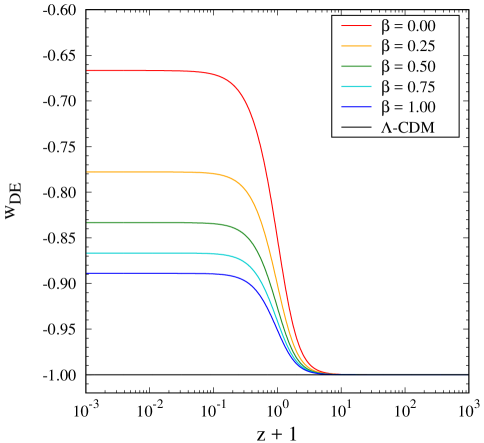
Figure 1: Evolution of $w_{\rm DE}$ versus $z+1$ for the exponential potential $V=V_{0}e^{-\lambda\phi/M_{\rm pl}}$ with $\lambda=1$ and five different values of $\beta$. We also plot the evolution of $w_{\rm DE}$ for the $\Lambda$CDM model (black line). The initial conditions are chosen to be $x_{1}=10^{-13}$, $x_{2}=10^{-14}$, $\Omega_{r}=0.999966$, and $\Omega_{b}=5.3\times 10^{-6}$ around $z\simeq 10^{8}$, so that the present epoch ($z=0$) corresponds to $\Omega_{\rm DE}=0.68$, $\Omega_{r}\simeq 10^{-4}$, and $\Omega_{b}\simeq 0.05$.

V.2 Evolution of perturbations

We proceed to study the evolution of perturbations for the modes relevant to the growth of large-scale structures. Since the scalar potential $V$ is at most of order $M_{\rm pl}^{2}H^{2}$, the field mass squared $V_{,\phi\phi}$ can be estimated as $V_{,\phi\phi}=\lambda^{2}V/M_{\rm pl}^{2}\lesssim\lambda^{2}H^{2}$. To realize the late-time cosmic acceleration, we consider the potential whose slope is in the range $|\lambda|\lesssim{\cal O}(1)$. Then, the quantity (75) is at most of order $\mu_{M}\lesssim(aH/k)^{2}$, which is much smaller than 1 for perturbations deep inside the Hubble radius. Hence we set $\mu_{M}=0$ in the following discussion.

For the function (84), the gravitational couplings of CDM are given by $G_{cc}=G_{cb}=G/(1+r_{f})$, with

$$r_{f}=\frac{2\beta mx_{1}^{2}(1+2\beta)}{\Omega_{c}[1+\beta(2-m)]}=\frac{2\beta mx_{1}^{2}}{\Omega_{c}\hat{c}_{s}^{2}}\,,$$ (103)

where $\hat{c}_{s}$ is given by Eq. (90). Provided that the Laplacian instability of scalar perturbations is absent, the quantity $r_{f}$ is positive for $\beta m>0$. When $\beta>0$ and $m>0$, the other stability conditions (87) and (88) are also automatically satisfied. This means that, for positive $\beta$ and $m$ in the range $1+\beta(2-m)>0$, both $G_{cc}$ and $G_{cb}$ are smaller than $G$.

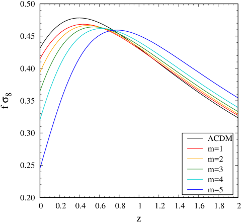
Figure 2: Evolution of $G_{cc}/G$ (left) and $f\sigma_{8}$ (right) for $\lambda=1$ and $\beta=1/4$ with five different values of $m$. The black lines correspond to the case of $\Lambda$CDM model. The background initial conditions are the same as those used in the simulation of Fig. 1. For perturbations, we consider the wavenumber $k=375a_{0}H_{0}$ with $\sigma_{8}(z=0)=0.811$.

In the left panel of Fig. 2, we plot the evolution of $G_{cc}/G$ for $\lambda=1$ and $\beta=1/4$ with five different values of $m$. Since the background dynamics is independent of $m$, the five cases shown in Fig. 2 give the same background evolution. For $\lambda$ and $\beta$ chosen in the simulation of Fig. 2 the quantity (103) reduces to $r_{f}=3x_{1}^{2}\Omega_{c}^{-1}m/(6-m)$, where $x_{1}$ and $\Omega_{c}$ are solely determined by the background. As the power $m$ increases in the range $0<m<6$, $r_{f}$ gets larger and hence $G_{cc}$ and $G_{cb}$ decrease. Indeed, this property can be confirmed in the numerical simulation of Fig. 2. If $m=0$, then the coupling (84) does not contain the $Z$ dependence, in which case $G_{cc}=G_{cb}=G$. The $Z$ dependence in $f$ allows the possibility for realizing the CDM gravitational coupling smaller than $G$. When $m=2$, which corresponds to the orange line in Fig. 2, our interacting model reduces to the scenario studied in Ref. Pourtsidou:2016ico . Even though the models with same $\beta$ and different $m$ give the same background evolution, the dynamics of perturbations strongly depends on $m$. In Fig. 2, we observe that, for $m>2$, $G_{cc}$ is smaller than in the case $m=2$ at low redshifts. Since the quantity (103) diverges in the limit $m\to 2+1/\beta$, the largest effect for reducing $G_{cc}$ and $G_{cb}$ occurs around $m=2+1/\beta$.

From Eqs. (77) and (78), the density contrasts of CDM and baryons obey

$$\delta_{c{\rm N}}^{\prime\prime}+\left(\frac{1}{2}-\frac{3}{2}w_{\rm eff}+c\right)\delta_{c{\rm N}}^{\prime}-\frac{3}{2}\frac{1}{1+r_{f}}\left(\Omega_{c}\delta_{c{\rm N}}+\Omega_{b}\delta_{b{\rm N}}\right)=0\,,$$ (104)

$$\delta_{b{\rm N}}^{\prime\prime}+\left(\frac{1}{2}-\frac{3}{2}w_{\rm eff}\right)\delta_{b{\rm N}}^{\prime}-\frac{3}{2}\left(\Omega_{c}\delta_{c{\rm N}}+\Omega_{b}\delta_{b{\rm N}}\right)=0\,,$$ (105)

where

$$c=\frac{2\sqrt{6}\lambda m\beta x_{1}x_{2}^{2}-6m\beta(1+2\beta)x_{1}^{2}}{\Omega_{c}[1+\beta(2-m)]+2m\beta(1+2\beta)x_{1}^{2}}\,.$$ (106)

During the deep matter era in which the scalar-field densities are suppressed relative to the CDM density ($x_{1}^{2}\ll\Omega_{c},x_{2}^{2}\ll\Omega_{c}$), the quantities $r_{f}$ and $c$ are much smaller than 1. In this regime, both $\delta_{c{\rm N}}$ and $\delta_{b{\rm N}}$ grow according to $\delta_{c{\rm N}}\propto\delta_{b{\rm N}}\propto a$. After the DE density dominates over the CDM density, the deviations of $r_{f}$ and $c$ from 0 tend to be significant. On the fixed point (100), we have $G_{cc}=G_{cb}\to 0$ and $c\to 3-\lambda^{2}/(1+2\beta)$. Under the condition (102), this asymptotic value of $c$ is larger than 1. Numerically, we confirmed that the coefficient $1/2-3w_{\rm eff}/2+c$ in front of the friction term $\delta_{c{\rm N}}^{\prime}$ in Eq. (104) remains positive during the transition from the matter era to the DE dominance.

For $r_{f}>0$ the CDM gravitational coupling $G/(1+r_{f})$ decreases from $G$ at low redshifts, so the growth rate of $\delta_{c{\rm N}}$ is smaller than that for $r_{f}=0$. The gravitational coupling of baryons is equivalent to $G$, but $\delta_{b{\rm N}}$ is affected by the CDM perturbation through the quantity $\Omega_{c}\delta_{c{\rm N}}$ in Eq. (105). Defining the total matter perturbation as $\delta\rho_{m{\rm N}}=\delta\rho_{c{\rm N}}+\delta\rho_{b{\rm N}}$ with the background density $\rho_{m}=\rho_{c}+\rho_{b}$, the corresponding density contrast is

$$\delta_{m{\rm N}}\equiv\frac{\delta\rho_{m{\rm N}}}{\rho_{m}}=\frac{\Omega_{c}}{\Omega_{m}}\delta_{c{\rm N}}+\frac{\Omega_{b}}{\Omega_{m}}\delta_{b{\rm N}}\,,$$ (107)

where $\Omega_{m}=\Omega_{c}+\Omega_{b}$. The growth rate of matter perturbations is given by $f\equiv\dot{\delta}_{m{\rm N}}/(H\delta_{m{\rm N}})=\delta_{m{\rm N}}^{\prime}/\delta_{m{\rm N}}$. Today’s values of CDM and baryon density parameters are $\Omega_{c}\simeq 0.27$ and $\Omega_{b}\simeq 0.05$, respectively, so the dominant contribution to $\delta_{m{\rm N}}$ comes from the CDM perturbation.

In the right panel of Fig. 2, we plot the evolution of $f\sigma_{8}$ for five different cases, where the Planck2018 best-fit value $\sigma_{8}(z=0)=0.811$ Aghanim:2018eyx is used in the simulation. For increasing $m$ the values of $f\sigma_{8}$ at low redshifts decrease, by reflecting the fact that $G_{cc}$ and $G_{cb}$ get smaller. In comparison to the $\Lambda$CDM model, our interacting model allows the possibility for alleviating the problem of $\sigma_{8}$ tension by reducing the values of $f\sigma_{8}$. Moreover, the model is sufficiently versatile in that almost any cosmic growth rate weaker than that in the $\Lambda$CDM model can be realized by appropriately choosing the values of $m$ and $\beta$.

In order to examine whether our interacting model is observationally favored over the $\Lambda$CDM model, we need to carry out the Markov-chain-Monte-Carlo simulation by varying $\sigma_{8}(z=0)$ besides other cosmological parameters instead of setting them to the Planck best-fit values of the $\Lambda$CDM. In this vein, Ref. Pourtsidou:2016ico studied observational constraints on the interacting DE and DM scenario with $f=\beta Z^{2}$, i.e., the power $m=2$. The joint analysis using CMB and galaxy clustering data showed that this particular model is favored over the $\Lambda$CDM model as a consequence of alleviating the $\sigma_{8}$ tension. Since the coupling (84) can realize almost any cosmic growth rate with the additional power $m$, it is of interest to explore how the latest data put observational constraints on our model. This interesting issue is left for a future work.

From Eqs. (76) and (107), the gravitational potentials are expressed as

$$\Psi=-\Phi\simeq-\frac{3}{2}\left(\frac{aH}{k}\right)^{2}\Omega_{m}\delta_{m{\rm N}}\,.$$ (108)

When $r_{f}>0$ the growth rate of $\delta_{m{\rm N}}$ is smaller than that for $r_{f}=0$, so the gravitational potentials in the former decay faster than those in the latter. Indeed, this property is confirmed in our numerical simulation. The suppressed gravitational potentials at low redshifts, together with the absence of gravitational slip, are key features for probing our model further from the observations of weak lensing.

VI Conclusions

We studied the cosmology of coupled DE and DM theories given by the action (2). The scalar derivative interaction with the CDM four velocity, which is weighed by the scalar combination $Z=u_{c}^{\mu}\partial_{\mu}\phi$, gives rise to several different features in comparison to the scalar field coupled to the CDM density of the form $f_{1}(\phi)\rho_{c}$. At the background level the coupling $f(X,Z)$ modifies the DE density and pressure in the forms (21) and (22), but the interacting terms do not explicitly appear on the right hands of DE and CDM continuity equations. This is attributed to the fact that the interaction between DE and DM in our scenario corresponds to the momentum transfer Pourtsidou:2013nha ; Pourtsidou:2016ico .

In Sec. III, we expanded the action (2) up to second order in scalar perturbations and derived the quadratic-order action in the form (32) with the Lagrangians (33) and (34). We then obtained the full linear perturbation equations of motion in the gauge-ready form. The gauge-invariant gravitational potentials $\Psi$ and $\Phi$ obey the relation (46), so there is no gravitational slip in our coupled DE and DM theories.

In Sec. IV, we derived conditions for the absence of scalar ghosts and Laplacian instabilities by eliminating nondynamical perturbations from the second-order action (32). In the small-scale limit, the no-ghost conditions are given by Eqs. (55) and (56). We showed that, provided $c_{c}^{2}=0$, the effective CDM sound speed squared $c_{\rm CDM}^{2}$ vanishes, so there is no additional pressure preventing the growth of CDM density perturbations. The Laplacian instability of the scalar degree of freedom is absent under the condition (64), where $c_{s}^{2}$ is given by Eq. (63) with Eq. (59). Applying the quasi-static approximation to the perturbations relevant to the growth of large-scale structures, we obtained the effective gravitational couplings felt by CDM and baryons in the forms (80) and (81), respectively. As long as the quantity $r_{f}$ defined by Eq. (82) is positive, the CDM gravitational couplings $G_{cc}$ and $G_{cb}$ are smaller than the Newton constant $G$.

In Sec. V, we studied the late-time cosmological dynamics for the explicit DE and DM coupling of the form (84). At the background level, the effect of interactions appears only through the derivative term $\beta\dot{\phi}^{2}$ in $\rho_{\rm DE}$ and $P_{\rm DE}$. For the exponential potential $V(\phi)=V_{0}e^{-\lambda\phi/M_{\rm pl}}$, the positive coupling $\beta$ leads to the dark energy equation of state closer to $-1$ relative to the uncoupled case. Provided that $1+\beta(2-m)>0$, the stability conditions (87)-(89) of scalar perturbations are satisfied for positive values of $\beta$ and $m$. Since $r_{f}>0$ in this case, the gravitational interaction with CDM is weaker than that for $\beta=0$. This property manifests itself in the suppressed growth of the total matter density contrast (107). For given values of $\beta$ and $\lambda$, $f\sigma_{8}$ tends to be smaller with the increase of $m$. As we observe in Fig. 2, this allows the suppressed growth rate of $\delta_{m{\rm N}}$ at low redshifts in comparison to the $\Lambda$CDM model.

We have thus shown that the dark-sector interaction $f(X,Z)$ provides an interesting possibility for realizing the cosmic growth rate weaker than that in the $\Lambda$CDM model. In comparison to the model $m=2$ studied in the literature, our interacting scenario with arbitrary powers of $m$ gives rise to a wide variety of perturbation dynamics which can be tested with observations. The coupling (84) may alleviate the tension of $\sigma_{8}$ between low- and high-redshift measurements by suppressing the values of $f\sigma_{8}$ in the range $z\lesssim 1$. It will be of interest to study in detail how much extent the coupling (84) reduces the tensions of $\sigma_{8}$ and $H_{0}$ present in the $\Lambda$CDM model. We leave observational constraints on our interacting model for a future work.

References

- (1) P. J. E. Peebles, Astrophys. J. 284, 439 (1984).
- (2) P. J. E. Peebles, Astrophys. J. 263, L1 (1982).
- (3) S. Weinberg, Rev. Mod. Phys. 61, 1 (1989).
- (4) A. G. Riess et al., Astrophys. J. 826, 56 (2016) [arXiv:1604.01424 [astro-ph.CO]].
- (5) N. Aghanim et al. [Planck Collaboration], arXiv:1807.06209 [astro-ph.CO].
- (6) L. Verde, T. Treu and A. G. Riess, Nature Astronomy, 3, 891-895 (2019) [arXiv:1907.10625 [astro-ph.CO]].
- (7) A. G. Riess, S. Casertano, W. Yuan, L. M. Macri and D. Scolnic, Astrophys. J. 876, no. 1, 85 (2019) [arXiv:1903.07603 [astro-ph.CO]].
- (8) W. L. Freedman et al., arXiv:1907.05922 [astro-ph.CO].
- (9) K. C. Wong et al., arXiv:1907.04869 [astro-ph.CO].
- (10) M. J. Reid, D. W. Pesce and A. G. Riess, Astrophys. J. 886, no. 2, L27 (2019) [arXiv:1908.05625 [astro-ph.GA]].
- (11) A. J. Shajib et al. [DES Collaboration], arXiv:1910.06306 [astro-ph.CO].
- (12) E. Macaulay, I. K. Wehus and H. K. Eriksen, Phys. Rev. Lett. 111, 161301 (2013) [arXiv:1303.6583 [astro-ph.CO]].
- (13) S. Nesseris, G. Pantazis and L. Perivolaropoulos, Phys. Rev. D 96, 023542 (2017) [arXiv:1703.10538 [astro-ph.CO]].
- (14) H. Hildebrandt et al., Mon. Not. Roy. Astron. Soc. 465, 1454 (2017) [arXiv:1606.05338 [astro-ph.CO]].
- (15) S. Joudaki et al., Mon. Not. Roy. Astron. Soc. 474, 4894 (2018) [arXiv:1707.06627 [astro-ph.CO]].
- (16) V. Salvatelli, N. Said, M. Bruni, A. Melchiorri and D. Wands, Phys. Rev. Lett. 113, 181301 (2014) [arXiv:1406.7297 [astro-ph.CO]].
- (17) S. Kumar and R. C. Nunes, Phys. Rev. D 94, 123511 (2016) [arXiv:1608.02454 [astro-ph.CO]].
- (18) S. Kumar and R. C. Nunes, Phys. Rev. D 96, 103511 (2017) [arXiv:1702.02143 [astro-ph.CO]].
- (19) E. Di Valentino, A. Melchiorri and O. Mena, Phys. Rev. D 96, 043503 (2017) [arXiv:1704.08342 [astro-ph.CO]].
- (20) R. An, C. Feng and B. Wang, JCAP 1802, 038 (2018) [arXiv:1711.06799 [astro-ph.CO]].
- (21) L. Kazantzidis and L. Perivolaropoulos, Phys. Rev. D 97, 103503 (2018) [arXiv:1803.01337 [astro-ph.CO]].
- (22) W. Yang, S. Pan, E. Di Valentino, R. C. Nunes, S. Vagnozzi and D. F. Mota, JCAP 1809, 019 (2018) [arXiv:1805.08252 [astro-ph.CO]].
- (23) S. Pan, W. Yang, E. Di Valentino, E. N. Saridakis and S. Chakraborty, arXiv:1907.07540 [astro-ph.CO].
- (24) E. Di Valentino, A. Melchiorri, O. Mena and S. Vagnozzi, arXiv:1908.04281 [astro-ph.CO].
- (25) W. Yang, S. Pan, R. C. Nunes and D. F. Mota, arXiv:1910.08821 [astro-ph.CO].
- (26) N. Dalal, K. Abazajian, E. E. Jenkins and A. V. Manohar, Phys. Rev. Lett. 87, 141302 (2001) [astro-ph/0105317].
- (27) W. Zimdahl and D. Pavon, Phys. Lett. B 521, 133 (2001) [astro-ph/0105479].
- (28) L. P. Chimento, A. S. Jakubi, D. Pavon and W. Zimdahl, Phys. Rev. D 67, 083513 (2003) [astro-ph/0303145].
- (29) B. Wang, Y. g. Gong and E. Abdalla, Phys. Lett. B 624, 141 (2005) [hep-th/0506069].
- (30) H. Wei and S. N. Zhang, Phys. Lett. B 644, 7 (2007) [astro-ph/0609597].
- (31) L. Amendola, G. Camargo Campos and R. Rosenfeld, Phys. Rev. D 75, 083506 (2007) [astro-ph/0610806].
- (32) Z. K. Guo, N. Ohta and S. Tsujikawa, Phys. Rev. D 76, 023508 (2007) [astro-ph/0702015 [astro-ph]].
- (33) M. B. Gavela, D. Hernandez, L. Lopez Honorez, O. Mena and S. Rigolin, JCAP 0907, 034 (2009) [arXiv:0901.1611 [astro-ph.CO]].
- (34) B. M. Jackson, A. Taylor and A. Berera, Phys. Rev. D 79, 043526 (2009) [arXiv:0901.3272 [astro-ph.CO]].
- (35) V. Faraoni, J. B. Dent and E. N. Saridakis, Phys. Rev. D 90, 063510 (2014) [arXiv:1405.7288 [gr-qc]].
- (36) N. Tamanini, Phys. Rev. D 92, 043524 (2015) [arXiv:1504.07397 [gr-qc]].
- (37) J. Valiviita, E. Majerotto and R. Maartens, JCAP 0807, 020 (2008) [arXiv:0804.0232 [astro-ph]].
- (38) J. Valiviita, R. Maartens and E. Majerotto, Mon. Not. Roy. Astron. Soc. 402, 2355 (2010) [arXiv:0907.4987 [astro-ph.CO]].
- (39) A. Pourtsidou, C. Skordis and E. J. Copeland, Phys. Rev. D 88, 083505 (2013) [arXiv:1307.0458 [astro-ph.CO]].
- (40) C. G. Boehmer, N. Tamanini and M. Wright, Phys. Rev. D 91, 123002 (2015) [arXiv:1501.06540 [gr-qc]].
- (41) C. G. Boehmer, N. Tamanini and M. Wright, Phys. Rev. D 91, 123003 (2015) [arXiv:1502.04030 [gr-qc]].
- (42) C. Skordis, A. Pourtsidou and E. J. Copeland, Phys. Rev. D 91, 083537 (2015) [arXiv:1502.07297 [astro-ph.CO]].
- (43) T. S. Koivisto, E. N. Saridakis and N. Tamanini, JCAP 1509, 047 (2015) [arXiv:1505.07556 [astro-ph.CO]].
- (44) A. Pourtsidou and T. Tram, Phys. Rev. D 94, 043518 (2016) [arXiv:1604.04222 [astro-ph.CO]].
- (45) J. Dutta, W. Khyllep and N. Tamanini, Phys. Rev. D 95, 023515 (2017) [arXiv:1701.00744 [gr-qc]].
- (46) R. Kase and S. Tsujikawa, Phys. Rev. D 101, 063511 (2020) [arXiv:1910.02699 [gr-qc]].
- (47) B. F. Schutz and R. Sorkin, Annals Phys. 107, 1 (1977).
- (48) J. D. Brown, Class. Quant. Grav. 10, 1579 (1993) [gr-qc/9304026].
- (49) D. Bettoni, S. Liberati and L. Sindoni, JCAP 1111, 007 (2011) [arXiv:1108.1728 [gr-qc]].
- (50) D. Bettoni and S. Liberati, JCAP 1508, 023 (2015) [arXiv:1502.06613 [gr-qc]].
- (51) A. De Felice, J. M. Gerard and T. Suyama, Phys. Rev. D 81, 063527 (2010) [arXiv:0908.3439 [gr-qc]].
- (52) A. De Felice, L. Heisenberg, R. Kase, S. Mukohyama, S. Tsujikawa and Y. l. Zhang, JCAP 1606, 048 (2016) [arXiv:1603.05806 [gr-qc]].
- (53) R. Kase and S. Tsujikawa, JCAP 1811, 024 (2018) [arXiv:1805.11919 [gr-qc]].
- (54) N. Frusciante, R. Kase, K. Koyama, S. Tsujikawa and D. Vernieri, Phys. Lett. B 790, 167 (2019) [arXiv:1812.05204 [gr-qc]].
- (55) S. Nakamura, R. Kase and S. Tsujikawa, JCAP 1912, 032 (2019) [arXiv:1907.12216 [gr-qc]].
- (56) B. J. Barros, Phys. Rev. D 99, 064051 (2019) [arXiv:1901.03972 [gr-qc]].
- (57) L. Amendola, Phys. Rev. D 60, 043501 (1999) [astro-ph/9904120].
- (58) Y. Fujii and K. Maeda, “The scalar-tensor theory of gravitation”, Cambridge University Press (2003).
- (59) C. Wetterich, Astron. Astrophys. 301, 321 (1995) [hep-th/9408025].
- (60) L. Amendola, Phys. Rev. D 62, 043511 (2000) [astro-ph/9908023].
- (61) B. Gumjudpai, T. Naskar, M. Sami and S. Tsujikawa, JCAP 0506, 007 (2005) [hep-th/0502191].
- (62) L. Amendola, M. Quartin, S. Tsujikawa and I. Waga, Phys. Rev. D 74, 023525 (2006) [astro-ph/0605488].
- (63) J. M. Bardeen, Phys. Rev. D 22, 1882 (1980).
- (64) J. c. Hwang and H. r. Noh, Phys. Rev. D 65, 023512 (2002) [astro-ph/0102005].
- (65) L. Heisenberg, R. Kase and S. Tsujikawa, Phys. Rev. D 98, 123504 (2018) [arXiv:1807.07202 [gr-qc]].
- (66) L. Heisenberg, M. Bartelmann, R. Brandenberger and A. Refregier, Phys. Rev. D 98, 123502 (2018) [arXiv:1808.02877 [astro-ph.CO]].
- (67) Y. Akrami, R. Kallosh, A. Linde and V. Vardanyan, Fortsch. Phys. 67, no. 1-2, 1800075 (2019) [arXiv:1808.09440 [hep-th]].