Quantile Factor Models††thanks: We are indebted to Ulrich Müller and four anonymous referees for their constructive inputs which have greatly improved the paper. We also thank Dante Amengual, Manuel Arellano, Steve Bond, Guillaume Carlier, Valentina Corradi, Jean-Pierre Florens, Alfred Galichon, Peter R. Hansen, Jerry Hausman, Sophocles Mavroeidis, Bent Nielsen, Olivier Scaillet, Enrique Sentana, Liangjun Su, and participants at several seminars and conferences for many helpful comments and suggestions. Financial support from the National Natural Science Foundation of China (Grant No.71703089), The Open Society Foundation, The Oxford Martin School, the Spanish Ministerio de Economía y Competitividad (grants ECO2016-78652 and Maria de Maeztu MDM 2014-0431), and MadEco-CM (grant S205/HUM-3444) is gratefully acknowledged. The usual disclaimer applies.
Abstract
Quantile Factor Models (QFM) represent a new class of factor models for high-dimensional panel data. Unlike Approximate Factor Models (AFM), where only location-shifting factors can be extracted, QFM also capture unobserved factors shifting other relevant parts of the distributions of observables. We propose a quantile regression approach, labeled Quantile Factor Analysis (QFA), to consistently estimate all the quantile-dependent factors and loadings. Their asymptotic distribution is derived using a kernel-smoothed version of the QFA estimators. Two consistent model-selection criteria, based on information criteria and rank minimization, are developed to determine the number of factors at each quantile. Moreover, in contrast to the conditions required by Principal Components Analysis in AFM, QFA estimation remains valid even when the idiosyncratic errors have heavy-tailed distributions. Three empirical applications (regarding climate, macroeconomic and finance panel data) illustrate that extra factors shifting quantiles other than the means could be relevant for causality analysis, prediction and economic interpretation of common factors.
Keywords: Factor models, quantile regression, incidental parameters.
JEL codes: C31, C33, C38.
1 Introduction
Following the key contributions by Ross (1976), Chamberlain and Rothschild (1983) and Connor and Korajczyk (1986) to the theory of approximate factor models (AFM henceforth) in the context of asset pricing, the analysis and applications of this class of models have proliferated thereafter. As it is well known, AFM imply that a panel of variables (units), each with observations, has the representation , where and are vectors of factor loadings and common factors, respectively, with , and are zero-mean weakly dependent idiosyncratic disturbances which are uncorrelated with the factors.
The fact that it is easy to construct theories involving common factors, at least in a narrative version, together with the availability of fairly straightforward estimation procedures for AFM— e.g. via Principal Components Analysis (PCA), has led to their extensive use in many fields of economics.111 Early applications of AFM abound in Aggregation Theory, Consumer Theory, Business Cycle Analysis, Finance, Monetary Economics, and Monitoring and Forecasting; see, inter alia, Bai (2003), Bai and Ng (2008b), Stock and Watson (2011). More recently, the characterization of cross-sectional dependence among error terms in Panel Data has relied on the use of a finite number of unobserved common factors which originate from economy-wide shocks affecting units with different intensities (loadings). Interactive fixed-effects models can be easily estimated by PCA (see Bai 2009) or by common correlated effects (see Pesaran 2006), and there are even generalizations of these techniques for nonlinear panel single-index models (see Chen et al. 2018). Lastly, the surge of Big Data and Machine Learning technologies has made factor models a key tool for dimension reduction and predictive analytics when using very large datasets (see Athey and Imbens 2019 for a survey).
Inspired by the generalization of linear regression to quantile regression (QR) models, our starting point in this paper is to claim that the standard regression interpretation of static AFM as linear conditional mean models of given (i.e. ), entails two possibly restrictive features. On the one hand, PCA does not capture hidden factors that may shift characteristics (moments or quantiles) of the distribution of other than its mean. On the other hand, neither the loadings nor the factors are allowed to vary across the distributional characteristics of each unit in the panel.
Highlighting these limitations, a growing literature in empirical finance has been documenting a much more pronounced co-movement of financial asset returns at the lower part than at the rest of their distributions. In particular, Amengual and Sentana (2018) reject the null hypothesis of a Gaussian copula when analyzing the cross-sectional dependence among monthly returns on individual US stocks, for which they find nonlinear tail dependence, co-skeweness and co-kurtosis. Likewise, Ando and Bai (2020) (AB 2020, hereafter) report that the common factor structures explaining the asset return distributions in global financial markets since the subprime crisis are different in the lower and the upper tails. In international finance, Maravalle and Rawdanowicz (2018) find that, while global and regional factors were key in explaining fluctuations of European government bond yields between the Great Moderation and the onset of the Great Recession (lower tails of the distributions of bond yields), their role decreased afterwards, giving way to country-specific factors as the main driving forces.222The diminishing role of the former factors could result from quantitative easing and the increase in yields (upper tail of the distribution), while the emergence of the latter factors could be due to the financial fragmentation in a number of vulnerable euro-area countries during sovereign debt crisis. On the macro side, Adrian et al. (2019) find that, while the estimated lower conditional quantiles of the distribution of future GDP growth in the US exhibit strong dependence on current financial conditions, the upper quantiles are stable over time. Lastly, in micro theory, de Castro and Galvao (2019) have recently extended the expected utility model of rational behavior to quantile utility preferences, where e.g. factor structures determining hedonic pricing of consumption goods or financial stocks may exhibit large differences across quantiles.
A simple way of illustrating the above limitations of the conventional formulation of AFM is to consider the factor structure in a location-scale shift model with the following Data Generating Process (DGP): , with (both are scalars), and . The first factor () shifts location, whereas the second factor () shifts the scale and therefore governs the volatility of shocks to . This model has been proposed by Herskovic et al. (2016) to empirically document a strong co-movement of the volatilities in the idiosyncratic component of individual stock returns and firm-level cash flows.333This DGP is further discussed in subsection 2.2 below, where we present a larger set of illustrative models as examples of potential DGPs for . Notice that the simplifying assumption of a known number of factors in this specific example is later relaxed. Such a DGP can be rewritten in QR format as , with , , where represents the quantile function of , , , and the conditional quantile .444Throughout the paper we use to denote the conditional quantile of given . PCA will only extract the location-shifting factor in this model, but it will fail to capture the scale-shifting factor and the quantile-dependent loadings in its QR representation. As will be explained below, our estimation procedure allows to estimate the space spanned by and .555Given that can be consistently estimated by PCA, it is also feasible to separate from their joint space. Also notice that, when the distribution of is symmetric, then can be considered as being quantile dependent, i.e. , since for , and for . Together with the remaining examples discussed below, this means that the general class of models to be considered in the sequel would be one where the loadings, factors and the number of factors are all allowed to be quantile-dependent objects, namely, , and for . In what follows, we coin this class of models Quantile Factor Models (QFM, hereafter), whose detailed definition is provided in Section 2 below.
That said, our goal in this paper is to develop a common factor methodology for QFM which is flexible enough to capture the quantile-dependent objects that standard AFM tools fail to recover. To do so, we analyze their estimation and inference, including selection criteria for the number of factors at each quantile . Put succinctly, QFM could be thought of as capturing the same type of flexible generalization that QR techniques represent for linear regression models.
To help understand how this new methodology works, we start by proposing an estimation approach for the quantile-dependent objects in QFM, labeled Quantile Factor Analysis (QFA, henceforth). Our QFA estimation procedure relies on the minimization of the standard check function in QR (instead of the conventional quadratic loss function used in AFM) to estimate jointly the common factors and the loadings at a given quantile , once the number of factors has been selected. However, since the objective function for QFM is not convex in the relevant parameters, we introduce an iterative QR algorithm which yields estimators of the quantile-dependent objects. We then derive their average rates of convergence, and propose two consistent selection criteria (one based on information criteria and another on rank minimization) for the number of factors at each . In addition, we establish asymptotic normality for QFA estimators based on smoothed QR (see e.g., Horowitz 1998 and Galvao and Kato 2016). Moreover, given that QFA estimation captures all quantile-shifting factors (including those affecting the means of observed variables), our asymptotic results and the proposed selection criteria provide a natural way to differentiate AFM from QFM.
In sum, the key contributions of this paper to the literature on factor models can be summarized as follows:
-
1.
We provide a complete asymptotic analysis for a new class of factor models: QFM. In particular, we show that the average convergence rates of the QFA estimators are the same as the PCA estimators of Bai and Ng (2002) (BN 2002, hereafter), which is a crucial result for proving the consistency of the two selection criteria of the number of factors at each . In addition, similar to Bai (2003), our QFA estimators based on smoothed QR are shown to converge at the parametric rates ( and ) to normal distributions.
-
2.
We argue that the problems of incidental parameters and non-smooth object functions require the use of some novel techniques in our proofs, which are borrowed from the theory of empirical processes. Moreover, our proof strategy can be easily extended to some other nonlinear factor models (e.g., probit and logit factor models considered by Chen et al. 2018) with smooth object functions. Finally, as a byproduct of our approach (and in exchange for some restrictions on the dependence of the idiosyncratic errors in an AFM; see Assumption 1 below), it is shown that the QFA estimators inherit from QR certain robustness properties to the presence of outliers and heavy-tailed distributions in those error terms, which would render PCA invalid.
-
3.
We show in the empirical section how QFA could provide a useful tool for quantile causal analysis, density forecasting, and economic interpretation of factors by applying the proposed methodology to three different datasets related to climate, macroeconomic aggregates and stock returns.
Related literature
There is a recent literature that attempts to make the AFM setup more flexible. For example, Su and Wang (2017) allow for the factor loadings to be time-varying and Pelger and Xiong (2018) admit these loadings to be state dependent. Chen et al. (2009) provide a theory for nonlinear PCA, where they favor sieve estimation to retrieve nonlinear factors. Finally, Gorodnichenko and Ng (2017) propose an algorithm to estimate level and volatility factors simultaneously. Different from these studies, our approach to modelling nonlinearities in factor models is through the conditional quantiles of the observed data.
On top of this, there is an emerging literature on heterogeneous panel quantile models with factor structures, especially in financial economics. The main idea is that a few unobservable factors explain co-movements of asset return distributions in a large range of asset returns observed at high frequencies, as in stock markets. In parallel and independent research, there have been two papers related to ours. First, Ma et al. (2019) propose estimation and inference procedures in semiparametric quantile factor models. In these models, factor loadings/betas are smooth functions of a small number of observables under the assumption that the included factors all have non zero mean. Then, sieve techniques are used to obtain preliminary estimation of these functions for each time period. Finally, the factor structure is imposed in a sequential fashion to estimate the factor returns by GLS under weak conditions on cross-sectional and temporal dependence. We depart from these authors in that we do not need to assume the loadings to depend on observables and, foremost, in that not only loadings but also factors are quantile-dependent objects in our setup. Second, in a closely related paper, AB (2020) use a similar setup to ours, where the unobservable factor structure is also allowed to be quantile dependent. These authors use Bayesian MCMC and frequentist estimation approaches, the latter building upon our proposed iterative procedure, as duly acknowledged in their paper. However, we differ from AB (2020) in several respects which make our QFA approach valuable: (i) our assumptions are less restrictive, since we rely on properties of the density, as in QR, while AB (2020) needs all the moments of the idiosyncratic errors to exist, (ii) our proofs of the main results are different from theirs, and (iii) our rank-minimization selection criterion to estimate the number of factors is novel, behaves well in finite samples and is computationally more efficient than the information criteria-based method.
Finally, it is noteworthy that the illustrative location-scale shift model above, where , is behind a current line of research in asset pricing which has been coined the “idiosyncratic volatility puzzle” by Ang et al. (2006). This approach focuses on the co-movements in the idiosyncratic volatilities of a panel of asset returns, and consists of applying PCA to (or taking cross-sectional averages of) the squared residuals, once the mean (PCA) factors have been removed from the original variables (a procedure labeled PCA-SQ hereafter).666See, e.g., Barigozzi and Hallin (2016), Herskovic et al. (2016) and Renault et al. (2017). Notice that the volatility co-movement does not arise from omitted factors in the AFM but from assuming a genuine factor structure in the idiosyncratic volatility processes. For example, this technique would be valid for our illustrative example above. Yet, while the QFA approach is able to recover the whole QFM structure for more general DGPs than the previous model (see subsection 2.2), PCA-SQ fails to do so. It will also fail when the idiosyncratic errors do not have bounded eighth moments. Hence, to the best of our knowledge, our QFA approach becomes the first estimation procedure capable of dealing with these issues.
Structure of the Paper
The rest of the paper is organized as follows. Section 2 defines QFM and provides a list of simple illustrative examples where the new QFM methodology applies. In Section 3, we present the QFA estimator and its computational algorithm, establish the average rates of convergence of the quantile-dependent factors and factor loadings, and propose two consistent selection criteria to choose the number of factors at each quantile. Section 4 introduces a kernel-smoothed version of the QFA estimators to derive their asymptotic distributions. Section 5 contains some Monte Carlo simulation results to evaluate the performance in finite samples of our estimation procedures relative to other alternative approaches with different assumptions about the idiosyncratic error terms. Section 6 considers three empirical applications using three large panel datasets, where we document the relevance of extra factors in causal analysis, forecasting and economic interpretation of common factors. Finally, Section 7 concludes and suggests several avenues for further research. Proofs of the main results are collected in the Online Appendix.
Notations
The Frobenius norm is denoted as . For a matrix A with real eigenvalues, denotes the th largest eigenvalue. Following van der Vaart and Wellner (1996), the symbol means “left side bounded by a positive constant times the right side” (the symbol is defined similarly), and denotes the packing number of space endowed with semimetric .
2 The Model and Some Illustrative Examples
This section starts by introducing the main definitions to be used throughout the paper. Next, we show how to derive the QFM representation of several illustrative DGPs exhibiting different factor structures.
2.1 Quantile Factor Models
Suppose that the observed variable with and , has the following QFM structure at some :
where the common factors is a vector of unobservable random variables, is a vector of non-random factor loadings with . Note that in the QFM defined above, the factors, the loadings, and the number of factors are all allowed to be quantile-dependent.
Alternatively, the above equation implies that
| (1) |
where the quantile-dependent idiosyncratic error is assumed to satisfy the following quantile restrictions:
2.2 Examples
In this section we provide a few illustrative examples of how QFMs can be derived from different specifications of location-scale shift models and related ones. The goal of these simple illustrations is to show instances where the standard AFM methodology may fail to capture the full factor structure, therefore requiring the use of the alternative QFM approach.
Example 1.
Location-shift model. , where are zero-mean i.i.d errors independent of with cumulative distribution function (CDF) . Let be the quantile function of . Moreover, assume that the median of is 0, i.e., , then this simple model has a QFM representation (1) by defining , for , and , for . However, note that the standard estimation method (PCA) for this AFM may not be consistent if the distribution of has heavy tails. For example, Assumption C of BN (2002) requires , which is not satisfied if, e.g. follows the standard Cauchy or some Pareto distributions.
Example 2.
Location-scale shift model (same sign-restricted factor). , where for all and are defined as in Example 1. This model has a QFM representation (1) by defining and for all , such that the loadings of the factor are the only quantile-dependent objects.
Example 3.
Location-scale shift model (different factors). , where are defined as in Example 1, , , and . When and do not share common elements, this model has a QFM representation (1) with , for , and , for .
Example 4.
Location-scale shift model with an idiosyncratic error and its cube. , where is a standard normal random variable whose CDF is denoted as . Let be positive, then has an equivalent representation in form of (1) with , for , and , for . In particular, if for all and noticing that the mapping is strictly increasing, then we have for , so that there exists a QFM representation (1) with and for . Notice that in this case, the second factor in , , is quantile dependent even for .
Not surprisingly, the standard AFM methodology based on PCA only works in Example 1, insofar as the idiosyncratic errors satisfy certain moment conditions. In the remaining examples, PCA will only yield consistent estimates of those factors shifting the locations; however (except in Example 2), it will fail to capture those extra factors which shift quantiles other than the means, or their corresponding quantile-varying loadings. In the sequel, QFA is therefore proposed as a new estimation procedure to estimate both sets of quantile-dependent objects in QFM.
3 Estimators and their Asymptotic Properties
To simplify the notations, we suppress hereafter the dependence of and on , so that the QFM in (1) is rewritten as:
| (2) |
where . Suppose that we have a sample of observations generated by (2) for and , where the realized values of are and the true values of are . We take a fixed-effects approach by treating and as parameters to be estimated, and our asymptotic analysis is conditional on . In Section 3.1, we consider the estimation of and while is assumed to be known. Finally, Section 3.2 deals with the estimation of for each quantile.
3.1 Estimating Factors and Loadings
It is well known in the literature on factor models that and cannot be separately identified without imposing normalizations (see BN 2002). Without loss of generality, we choose the following normalizations:
| (3) |
Let , , and denotes the vector of true parameters, where we also suppress the dependence of and on to save notation. Let and define:
Further, define:
where is the check function. The QFA estimator of is defined as:
It is obvious that the way in which our estimator is related to the PCA estimator studied by BN (2002) and Bai (2003) is analogous to how QR is related to standard least-squares regressions. However, unlike Bai (2003)’s PCA estimator, our estimator does not yield an analytical closed form. This makes it difficult not only to find a computational algorithm that would yield the estimator, but also the analysis of its asymptotic properties. In the sequel, we introduce a computational algorithm called iterative quantile regression (IQR, hereafter) that can effectively find the stationary points of the object function. In parallel, Theorem 1 shows that achieves the same convergence rate as the PCA estimators for AFM.
To describe the algorithm, let , , and define the following averages:
Note that we have . The main difficulty in finding the global minimum of is that this object function is not convex in . However, for given , happens to be convex in for each and likewise, for given , is convex in for each . Thus, both optimization problems can be efficiently solved by various linear programming methods (see Chapter 6 of Koenker 2005). Based on this observation, we propose the following iterative procedure:
Iterative quantile regression (IQR):
Step 1: Choose random starting parameters: .
Step 2: Given , solve for ; given , solve for .
Step 3: For , iterate the second step until is close to , where .
Step 4: Normalize and so that they satisfy the normalizations in (3).
To see the connection between the IQR algorithm and the PCA estimator of Bai (2003), suppose that , and replace the check function in the IQR algorithm by the least-squares loss function. Then, it is easy to show that the second step of the algorithm above yields and , where is the matrix with elements , and . Thus, with proper normalizations at each step, the iterative procedure is equivalent to the well-known power method of Hotelling (1933), and the sequence will converge to the eigenvector associated with the largest eigenvalue of . In the more general case , if we replace the check function in the IQR algorithm by the least-squares loss function and normalize to satisfy (3) at step 2, it can be shown that the above iterative procedure is similar to the method of orthogonal iteration (see Section 7.3.2 of Golub and Van Loan 2013) for calculating the eigenvectors associated with the largest eigenvalues of , which is the PCA estimator of Bai (2003). Therefore, the IQR algorithm and its corresponding QFA estimator can be viewed as an extension of PCA to QFM.
Similar algorithms have been proposed in the machine learning literature to reduce the dimensions for binary data, where the check function is replaced by some smooth nonlinear link functions, e.g. Collins et al. (2001). However, unlike PCA, whether such methods guarantee finding the global minimum remains an important open question. Nonetheless, in all of our Monte Carlo simulations we found that the QFA estimators of the factors using the IQR algorithm always converge to the space of the true factors, which is somewhat reassuring in this respect.
To prove the consistency of the QFA estimator , we make the following assumptions:
Assumption 1.
(i) and are compact sets and . In particular,
with , and as for
with .
(ii) The conditional density function of given , denoted as , is continuous, and satisfies that: for any compact set and any , there exists a positive constant (depending on ) such that for all .
(iii) Given , is independent across and .
Assumptions 1 (i) is essentially the strong factors assumption that is standard in the literature (see Assumption B of Bai 2003). The requirement that are distinct is similar to Assumption G of Bai (2003), which is a convenient assumption to order the factors. Assumptions 1 (ii) and (iii) are similar to (C1) and (C2) in AB (2020), except that we do not require moments of to exist. Also notice that Assumption (iii), which allows for both cross-sectional and time series heteroskedasticity, requires the idiosyncratic errors to be mutually independent. This stems from the use of Hoeffding’s inequality in the proofs of some results, which provides a sub-Gaussian tail bound for the sum of bounded independent random variables. There have been attempts to relax this assumption (see Remark 1.4 below) but it is difficult to characterize the minimal set of conditions that the error terms should satisfy to achieve the sub-Gaussian inequality required in our proofs. Notice, however, that in exchange for the independence assumption, we can dispense with the bounded moment conditions in the idiosyncratic terms, whose violation would render PCA invalid. At any rate, in sub-section 5.2 we run some Monte Carlo simulation on the performance of our QFA estimation when error terms are allowed to exhibit mild cross-sectional and serial dependence in order to check the robustness of our results to these features.
Write , , , , and let . The following theorem provides the average rate of convergence of and .
Theorem 1.
Under Assumption 1, there exists a diagonal matrix whose diagonal elements are either or , such that as ,
The sign matrix appears in the above result due the intrinsic sign indeterminacy of factors and loadings – that is, the factor structure remains unchanged if a factor and its loading are both multiplied by (e.g., see Theorem 1.b of Stock and Watson 2002 for a similar result).
Remark 1.1: Since our proof strategy is substantially different from that of BN (2002), we briefly sketch the main ideas underlying our proof here. To facilitate the discussion, for any define the semimetric by:
and let
The semimetric plays an important role in our asymptotic analysis. We first show that . Next, it can be shown that:
| (4) |
and that for sufficiently small ,
| (5) |
where . Intuitively, the above two inequalities and imply that , or . Then, the desired results follow from the fact that .
Inequality (4) follows easily from a Taylor expansion of around , together with Assumption 1(ii). It is worth stressing that the proof of (5) requires the chaining argument which is commonly used in the theory of empirical processes. In particular, using Hoeffding’s inequality and the fact that , it can be shown that, for any given ,
| (6) |
for some constant . Then, along the lines of Theorem 2.2.4 of van der Vaart and Wellner (1996), it follows that the left-hand side of (5) is bounded (up to a positive constant) by . Finally, we can prove that , from which inequality (5) follows.
Remark 1.2: Compared to BN (2002), recall that, in exchange for Assumption 1(iii) we do not require any moment of to be finite. Thus, for the canonical AFM (e.g., Example 1) where the idiosyncratic errors have median equal to zero and satisfy Assumption 1(iii), our estimator for the case can be interpreted as a least absolute deviation (LAD) estimator which is robust to heavy tails and outliers. In relation to this issue, it is important to point out that the LAD estimator is related to robust PCA in the machine learning literature that aims to recover a low rank matrix from a large panel of observables. For example, the Principal Components Pursuit method proposed by Candès et al. (2011) features a combination of the norm (as in LAD) and a nuclear norm on the low rank matrix (see Chapter 3 of Vidal et al. 2016 and Bai and Ng 2019 for other robust PCA methods). In section 5 below, we will illustrate the robustness of the LAD estimator relative to the PCA estimator by Monte Carlo simulations.
Remark 1.3: If the true parameters do not satisfy the normalizations (3), they can still be in the space after some normalizations. Let be a invertible matrix and define , . Note that . For and to satisfy the normalizations (3), we require:
where , , and is a diagonal matrix with non-increasing diagonal elements. The above equalities imply that:
Thus, the rotation matrix can be chosen as , where is the matrix of eigenvectors of . Note that when the eigenvalues of are distinct, its eigenvectors are unique up to signs, i.e., each eigenvector can be replaced by the negative of itself. As a result, Theorem 1 can be stated as follows:
where is the diagonal matrix defined above. Notice that the rotation matrix is slightly different from the rotation matrix of Bai (2003). Moreover, because both and are -dependent, also varies across quantiles, although we did not make it explicitly quantile dependent in the previous discussion to simplify notation.
Remark 1.4: Compared to BN (2002), our Assumption 1(iii) is admittedly strong. However, note that this assumption is made conditional on , so cross-sectional and temporal dependence of due to the common factors are still allowed for. Moreover, the independence assumption is only used to establish the sub-Gaussian inequality (6). Thus, Assumption 1(iii) can be relaxed as long as the sub-Gaussian inequality holds.777See van de Geer (2002) for the properties of Hoeffding inequalities for martingales.
3.2 Selecting the Number of Factors
In the previous section, we assumed the number of quantile-dependent factors to be known at each . In this subsection we propose two different procedures to select the correct number of factors at each quantile with probability approaching one. The first one selects the number of factors by rank minimization while the second one uses information criteria (IC). As before, the dependence of the quantile-dependent objects on , including , is suppressed for notational simplicity.
3.2.1 Model Selection by Rank Minimization
Let be a positive integer larger than , and and be compact subsets of . In particular, let us assume that for all .
Let for all and write , , . Consider the following normalizations:
| (7) |
Define , and
Moreover, define and write
The first estimator of the number of factors is defined as:
where is a sequence that goes to 0 as . In other words, is equal to the number of diagonal elements of that are larger than the threshold . We call the rank-minimization estimator because, as discussed below in Remark 2.1, it can be interpreted as a rank estimator of .
It can then be shown that:
Theorem 2.
Under Assumption 1, as if , and .
Remark 2.1: In the proof of Theorem 2, we show that for , it holds that (up to sign)
where is the first columns of and . It then follows from Assumption 1 that for and for . Thus, the first diagonal components of converge in probability to positive constants while the remaining diagonal components are all . In other words, converges to a matrix with rank , and can be viewed as a cutoff value to choose the asymptotic rank of .
3.2.2 Model Selection by Information Criteria
The second estimator of is similar to the IC-based estimator of BN (2002). Let denote a positive integer smaller or equal to , and and be compact subsets of . In particular, for , assume that for all . Moreover, we can define and in a similar fashion.
Define the IC-based estimator of as follows:
We can show that:
Theorem 3.
Suppose Assumption 1 holds, and assume that for any compact set and any , there exists (depending on ) such that for all . Then as if , and .
Remark 3.1: AB (2020) obtain a similar result, but the difference with ours is that we only need the density function of the idiosyncratic errors to be uniformly bounded above and below, while AB (2020) requires all the moments of the errors to be bounded. The reason why we can obtain the same result here with less restrictions is that our proof is based on the innovative argument discussed in Remark 1.1 and on the average convergence rate of the estimators, while the proof of AB (2020) depends on the uniform convergence rate of the estimators.
Remark 3.2: Let denote the matrix of observed variables, and let denote the matrices of PCA estimators of BN (2002) when the number of factors is specified as . Then BN (2002)’s estimator of can be written as:
, and is defined as in Theorem 2 above. It can be shown that IC-based estimator is equivalent to the number of diagonal elements in that are larger than . Thus, the two seemly different estimators of the number of factors are equivalent in AFM. However, due to the differences of the object functions, such equivalence does not exist in QFM.
Remark 3.3: The choice of for and can be different in practice. In particular, it can differ from those penalties used by BN (2002). AB (2020) choose
for , similar to of BN (2002). However, as shown in AB’s (2020) simulation results, this choice does not perform very well even for as large as 300.
Remark 3.4: Even though and are both consistent estimators of , the computational cost of is much lower than that of , because for we only estimate the model once, while for we need to estimate the model times. Thus, in the simulations and empirical applications we will focus on , and we refer to AB (2020) for the corresponding simulation results of . In particular, we find that the choice
for works fairly well as long as is 100. This is also the value used in all of our simulations and applications.
4 Estimators Based on Smoothed Quantile Regressions
The derivation of the asymptotic distribution of the QFA estimator becomes a difficult task due to the non-smoothness of the check function and the problem of incidental parameters. As in the asymptotic analysis of conventional QR, one can expand the expected score function (which is smooth and continuously differentiable) and obtain a stochastic expansion for ; yet the following term appears in the expansion:
| (8) |
The next step would be to show that the above expression is a higher-order term (i.e. ) thus it does not affect the asymptotic distribution of . However, due to the presence of the indicator functions in (8), this is not an easy task. To see this, let’s consider a similar problem for the PCA estimators of AFM. Let and be the PCA estimators. In the stochastic expansion of , the analogous term to (8) happens to be:
where is the idiosyncratic error in the AFM. Note that, based on the result , one can only show that:
Instead, one has to use the stochastic expansion of to show that (see the proof of Lemma B.1 of Bai 2003). Likewise, to show that (8) is , establishing the convergence rate of is not enough, and the stochastic expansion of is required. However, due the non-smoothness of the indicator functions, it is not clear how to explore this stochastic expansion in (8).
To overcome this problem, we proceed to define a new estimator of , denoted as , relying on the following smoothed quantile regressions (SQR):
where
, is a continuous function with support , and is a bandwidth parameter that goes to 0 as diverge.
Define
for all . We impose the following assumptions:
Assumption 2.
Let be a positive integer,
(i) and for all .
(ii) is an interior point of and is an
interior point of for all .
(iii) is symmetric around and twice continuously
differentiable. , for and .
(iv) is times continuously differentiable. Let for . For any compact set and any , there exists such
that and for and
for all .
(v) As , , and .
The above conditions are standard in SQR, with the exception of . Note that, like Galvao and Kato (2016), we need to be a higher-order kernel function to control the higher-order terms in the stochastic expansions of the estimators. However, Galvao and Kato (2016) assume that (or ), while we need (or ). The difference is due to the fact that the incidental parameters ( and ) in QFM enter the model interactively, while in the panel quantile models considered by these authors there are no interactive fixed-effects.
Then, we can show that:
Theorem 4.
Under Assumptions 1 and 2, there exists a diagonal matrix whose diagonal elements are either or , such that
for each and , where .
Remark 4.1: Similar to the proof of Theorem 1, we can show that
where the extra term is due the approximation bias of the smoothed check function. However, Assumption 2 implies that , and then it follows that average convergence rates of and are both .
Remark 4.2: Similar to Theorems 1 and 2 of Bai (2003), we show that the new estimator is free of incidental-parameter biases. That is, the asymptotic distribution of is the same as if we would observe , and likewise the asymptotic distribution of is the same as if were observed. The proof of this result is not trivial. To see why this is the case, first define and , then we can write . Expanding around yields
| (9) |
where . The key step is to show that the last two terms on the right-hand side of the above equation are both . This is relatively easier for the PCA estimator of Bai (2003), since has an analytical form (like e.g. in equation A.1 of Bai 2003). In our case, we would also need a stochastic expansion for , which in turn depends on the stochastic expansion of due to the nature of factor models. As in Chen et al. (2018), this problem can be partly solved by showing that the expected Hessian matrix is asymptotically block-diagonal (see Lemma 11 in the Online Appendix). However, the proof of Chen et al. (2018) is only applicable to a special infeasible normalization, namely , while our proof of Lemma 11 allows for normalization (3) and can be generalized to any of the other normalizations considered by Bai and Ng (2013) that uniquely pin down the rotation matrix.
Remark 4.3: As discussed in Remark 1.3, if the true parameters do not satisfy the normalizations (3), the results of Theorem 3 can be stated as
where and are defined in Remark 1.3, , , , and is the matrix of eigenvectors of .
Remark 4.4: Let be a continuous kernel function with support where exists and is bounded for . Let a bandwidth. Estimators for the asymptotic variance matrices of and can be simply constructed as
and
with . In Section A.5 of the Online Appendix we show that under Assumptions 1 and 2, the above estimators of the asymptotic covariance matrices are consistent if and . Note that this is different from the usual condition in standard quantile regressions (see e.g. Powell 1984 and Angrist et al. 2006). Moreover, the above estimators are also consistent for the asymptotic covariance matrices discussed in Remark 4.3.
Remark 4.5: A restrictive DGP within class (1) would be a QFM where the PCA factors coincide with the quantile factors and only the factor loadings are quantile dependent. The representation for such restricted subset of QFM is as follows:
| (10) |
As a result, the main objects of interest are the common factors and the quantile-varying loadings. Notice that, if the factors were to be observed, using standard QR of on would lead to consistent and asymptotically normally distributed estimators of for each and . However, since are not observable, a feasible two-stage approach is to first estimate the factors by PCA, denoted as , and next run QR of on to obtain estimates of as follows:
| (11) |
As explained in Chen et al. (2017), unlike the QFA estimators (see Remark 1.2), this two-stage procedure requires moments of the idiosyncratic term to be bounded in order to apply PCA in the first stage. However, an interesting result (see Chen et al. 2017, Theorem 2) is that the standard conditions on the relative asymptotics of and allowing for the estimated factors to be treated as known do not hold when applying this two-stage estimation approach. In effect, while these conditions are for linear factor-augmented regressions (see Bai and Ng 2006) and for nonlinear factor-augmented regressions (Bai and Ng 2008a), lack of smoothness in the object (check) function at the second stage requires the stronger condition . Moreover, Theorem 3 in Chen et al. (2017) shows how to run inference on the quantile-varying loadings (e.g., testing the null that they are constant across all quantiles or a subset of them).
5 Finite Sample Simulations
In this section we report the results from several Monte Carlo simulations regarding the performance of our proposed QFM methodology in finite samples. In particular, we focus on four relevant issues: (i) how well does our preferred estimator of the number of factors perform relative to other methods when the distribution of the idiosyncratic errors in an AFM exhibits heavy tails or outliers, (ii) how well do PCA and QFA estimate the true factors under the previous circumstances, (iii) how robust is the QFA estimation procedure when the errors terms are serially and cross-sectionally correlated, instead of being independent, and (iv) how good are the normal approximations given in Theorem 4 for the QFA estimators based on SQR.
5.1 Estimation of AFM with Outliers
As pointed out in Remark 1.2, since the consistency of our QFA estimator does not require the moments of the idiosyncratic errors to exist, at it can be viewed as a robust QR alternative to the PCA estimators commonly used in practice. For the same token, our estimator of the number of factors should also be more robust to outliers and heavy tails than the IC-based method of BN (2002). In this subsection we confirm the above claims by means of Monte Carlo simulations.
We consider the following DGP:
where , , , are all independent draws from , and , where are i.i.d Bernoulli random variables with means equal to and denotes the standard Cauchy distribution. In this way, approximately of the idiosyncratic errors are generated as outliers.
We consider four estimators of the number of factors : two estimators based on , of BN (2002), the Eigenvalue Ratio (ER) estimator proposed by Ahn and Horenstein (2013) and our rank-minimization estimator discussed in subsection 3.2, having chosen
We set for all four estimators, and consider .
Table 1 reports the following fractions:
for each estimator having run 1000 replications.
It becomes evident from the results in Table 1 that and almost always overestimate the number factors, while the ER estimator tends to underestimate them, though to a lesser extent than what and overestimate them. By contrast, our rank-minimization estimator chooses accurately the right number of factors as long as .
Next, to compare the PCA and QFA estimators of the common factors in the previous DGP, we assume that is known. We first get the PCA estimator (denoted as ), and then obtain the QFA estimator at (denoted ) using the IQR algorithm. Next, we regress each of the true factors on and separately, and report the average from 1000 replications in Table 2 as an indicator of how well the space of the true factors is spanned by the estimated factors.888All the we use in this section and the next section are adjusted . As shown in the first three columns of Table 2, while the PCA estimators are not very successful in capturing the true common factors, the QFA estimators approximate them very well, even when are not too large.
As discussed earlier, the overall findings reported in Tables 1 and 2 are in line with our theoretical results. In effect, while the standard PCA estimators of BN (2002) fail to capture the true factors because they require the eighth moments of all the idiosyncratic errors to be bounded (unlike the DGP above), our QFA estimators succeed to do so since they only need the density function to exist and be continuously differentiable, like in the previous DGP. Thus, this simulation exercise provides strong evidence about the substantial gains that can be achieved by using QFA rather than PCA in those cases where the idiosyncratic error terms in AFM exhibit heavy tails and outliers.
5.2 Estimation of QFM: Heavy-tailed and Dependent Idiosyncratic Errors
In this subsection we consider the following DGP:
where , , , are all independent draws from , and are independent draws from . Following BN (2002), the following specification for is used:
where are independent draws from except in the second case below. The autoregressive coefficient captures the serial correlation of , while the parameters and capture the cross-sectional correlations of . We consider four cases:
-
Case 1:
Independent errors: and .
-
Case 2:
Independent errors with heavy tails: , and .
-
Case 3:
Serially correlated errors: and .
-
Case 4:
Serially and cross-sectionally correlated errors: and , and .
For each of the previous cases and each , we first estimate using our rank-minimization estimator, having set and as described in the previous subsection. Second, we estimate factors by means of the QFA estimation approach, which we denote . Finally, we regress each of the true factors on and calculate the s. This procedure is repeated 1000 times where, for each , we report the averages of and the s in these 1000 replications.
The results for Case 1 and Case 2 (where the heavy tails are captured this time by a Student(3) rather than by a Cauchy distribution) are reported in Table 3 and Table 4, respectively, for . Notice that for , we have while, for , we get , since the factor does not affect the median of . It can be observed that both our selection criterion and the QFA estimators perform very well in choosing the number of QFA factors and in estimating them. It should be noticed that at the estimation of the scale factor is not as good as the mean factors for small and . However, such differences vanish as and increase.
The results for Case 3 and Case 4 are in turn reported in Table 5 and Table 6, respectively. It can be inspected that the QFA estimators still perform well, even though the independence assumption is violated in these DGPs. Thus, despite adopting independence in Assumption 1 (iii) for tractability in the proofs (see Remark 1.4), it seems that QFA estimation still works properly when the error terms are allowed to exhibit mild serial and cross-sectional correlations.
5.3 Normal Approximations of the Estimators Based on SQR
To evaluate the normal approximations of Theorem 4 for the estimators based on SQR, we consider the following DGP:
where and they are normalized such that , and . Note that since our Theorem 4 is conditional on the factors and the loadings, and are fixed in the simulations. To smooth the indicator function, we use the following eighth-order kernel function (see Muller, 1984):
while the Epanechnikov kernel is applied to estimate the variance.
Figure 1 and Figure 2 plot the histograms of the standardized estimators of the factors: at , from 1000 replications999We choose the signs of such that ., where is estimated using the formula in Remark 4.4. To check how the bandwidths affect the finite distributions of the estimators, we display results for different choices of and .
From the reported histograms of the standardized estimators and the superimposed density function of the standard normal distribution, it becomes clear that the asymptotic distributions given in Theorem 4 provide reasonably good approximations for the finite sample distributions of the estimators based on SQR, even for , and that such approximations are not very sensitive to the choice of bandwidths.
6 Empirical Applications
In this section we argue that QFA could provide a useful tool for causal analysis, predictive exercises and the economic interpretation of factors. In particular, we focus on applying our proposed methodology to three different datasets related to climate, macro aggregates and stock returns.
6.1 Climate Change and Emissions
In our first empirical application we investigate how emissions affect temperatures, which is a long-standing issue in climate change science and economics (see e.g. Hansen et al. 1981, and Hsiang and Kopp 2018). The dataset (coined Climate for short) we use consists of the annual changes of temperature from 441 stations from 1917 to 2018 (), drawn from the Climate Research Unit at the University of East Anglia, where information about global temperatures across different stations in the Northern and Southern Hemisphere is collected. The annual global emissions data is downloaded from The Global Change Data Lab.
Table 7 (column labeled Climate) reports the estimated number of factors using of BN (2002), the ER estimator and the rank-minimization estimator for a grid of quantiles ranging from 0.01 to 0.99.101010In all the applications, before estimating the factors and the number of factors, each variable is standardized to have zero mean and variance equal to one. The maximum number of factors is set to for all estimators. selects the maximum number of factors (8), while the ER estimator selects only one. Thus, the tendencies to overestimate (resp. underestimate) the number of PCA factors by the former (resp. latter) criteria mirror our simulation results in Section 5.1. By contrast, it can be observed that the numbers of factors estimated by the rank-minimization vary across quantiles. In particular, the number of QFA factors decreases as we move away from the median.
To compare the QFA factors (denoted as ) and the PCA factors (denoted as ), we regress each element of on the 8 PCA factors selected by and compute the in these regressions.111111We choose the number of PCA factors estimated by in these regressions to play conservative. The results are shown in the upper panel of Table 8, where it becomes clear that the median factors () are highly correlated with the PCA factors, with all the s above . By contrast, the QFA factors at the upper and lower quantiles () exhibit much lower correlations with the PCA factors, with s around . Thus, there seems to be room for using QFA in this application.
Next, to analyze the impact of emissions on climate change, bivariate Granger non-causality tests are implemented. We regress the QFA factors at each relevant quantile on their own lags and the lagged growth rates of emissions, labeled , where the lag length is chosen according to BIC. Table 9 reports the p-values of these tests. The results of this novel approach to analyze quantile causality indicate that the growth rate of emissions strongly Granger causes the QFA factors at the lower quantiles (), with p-values below 0.01, as well as some of the median factors, albait to a lessser extent (p-values below 0.04). Moreover, the null of Granger non-causality is not rejected for QFA factors at the upper quantiles. Given that emissions lead to global warming, the results for the lower quantiles of temperatures are in line with the evidence reported by Gadea and Gonzalo (2020). Using a similar climate dataset but different quantile techniques to ours, these authors find that global warming over the last century seems to be mainly due to a different behaviour in the lower tail than in the central and upper tails of the distribution of global temperatures.
6.2 Macroeconomic Forecasting in a Data-Rich Environment
In the second application, we extend the diffusion-index forecasting exercise popularized by Stock and Watson (2002) to explore the predictive power of the QFA factors. The main goal is to extract a few common factors (by both PCA and QFA) from a large panel of macroeconomic variables, and then use these factors to forecast e.g. real GDP growth and the inflation rate.
The FRED-QD dataset (coined Macro here) is used to estimate PCA and QFA factors. This is a quarterly panel consists of 211 US macroeconomic variables from 1960Q1 to 2019Q2 (). It emulates the popular dataset used by Stock and Watson (2002), but also contains several additional time series. The variables in this dataset are updated in a timely manner and can be downloaded for free.121212Link to the dataset: http://research.stlouisfed.org/econ/mccracken/. We refer to McCracken and Ng (2016) for the details of a very similar dataset that contains monthly macroeconomic variables. Before estimation, each series is transformed to be stationary using Matlab codes that are also available on the FRED-QD data website.
As with the climate data, while selects 8 PCA factors, ER selects only one. The estimated numbers of QFA factors are reported in Table 7 (column labeled Macro). As can be seen, the number of QFA factors varies significantly across different quantiles, pointing to the existence of a nonstandard factor structure for this dataset. Moreover, the middle panel of Table 8 reports the s of regressing each of the QFA factors on the 8 PCA factors. It becomes clear that the QFA factors at close to are all well explained by the PCA factors. However, the first QFA factor at (denoted ) and those at (denoted as and ) contain some extra information that could be potentially helpful for forecasting macroeconomic variables. Since exhibits a very high correlation with and , we exclusively focus on the predictive power of and in the subsequent analysis.
Let denote the realized value of real GDP growth/inflation at period . The forecasting equation we consider is as follows:
where is vector containing several unobserved common factors extracted from the large macroeconomic dataset. The predicted value of , based on a vector of estimated factors , is simply constructed as , where are OLS estimates of the coefficients and is the optimal lag length according to BIC. We compare five different specifications for : (i) , which is the benchmark AR model, (ii) AR plus only including , (iii) AR plus including and , (iv) AR plus including and , and (v) AR plus including , and . Following Chudik et al. (2018), the initial estimation period is 1960Q1 to 1989Q4 (120 periods), and the forecast evaluation period is split into pre-crisis (1990Q1 to 2007Q2) and crisis and recovery (2007Q3 to 2019Q2) sub-periods. A rolling window of 120 periods is used both to estimate the coefficients and generate the rolling forecasts. In particular, following Chudik et al. (2018), the number of mean factors is estimated using at each rolling window, where the maximum number of factors is set equal to 5.
The mean squared error (MSE) of these procedures, and their relative MSE (R-MSE) to the benchmark AR model are reported in Table 10 for the whole evaluation period and each relevant sub-sample. As can be observed, in regards to real GDP growth, adding the upper tail QFA factors ranks better in terms of R-MSE than the AR and AR+ models for the three considered periods. The gains are not sizeable but yet they are relevant. As for the inflation rate, the results are weaker, though there are some gains for the crisis and recovery period.
A well-known shortcoming of point forecasts is that their uncertainty is generally unknown, hence it is difficult to quantify their precision at any given period of time. To address this problem, it has became customary among central banks to report density forecasts for important macroeconomic variables. In this respect, Adrian et al. (2019) argue that a simple way of producing such densities is via QR. Following these authors, we next evaluate the predictive power of the QFA factors for forecasting the densities of real GDP growth and inflation. In particular, we first predict the conditional quantiles of the target variable by for , where are estimated coefficients by running QR of on , and is a vector of estimated quantile factors using the IQR algorithm.131313Only 1 QFA factor is estimated at , whereas 5 QFA factors are estimated at . Next, given the predicted quantiles: , the predicted density of is constructed as the density of a skewed -distribution by matching the predicted quantiles.141414We refer to Adrian et al. (2019) for the details and to Azzalini and Capitanio (2003) for the definition and properties of the skewed -distribution. Finally, the accuracy of the density forecast is measured by the predictive score, which is the predicted density evaluated at the realized value of . Higher predictive scores indicate more accurate predictions. The out-of-sample density forecasts are constructed using rolling windows with the most recent 120 observations, and the evaluation period is 1990Q1 to 2019Q2. Moreover, we set , and the benchmark model is the one where , i.e. the quantiles of are predicted only using its own lags. Figure 3 displays the predictive scores of the one-quarter-ahead () and one-year-ahead () density forecasts for both variables. It can be seen that in both instances the predictive scores of the“AR + Quantile Factors” procedure is frequently above that of the “AR benchmark” model, sometimes by a large margin, indicating that the QFA factors could indeed be very informative for density forecasting of highly relevant macroeconomic variables.
6.3 Interpretation of Financial Factors
Our last application concerns the interpretation of the quantile factors extracted from financial asset returns. The dataset (Finance in short) contains the monthly returns of 429 stocks from 1980M01 to 2014M12 (), obtained from The Center of Research for Security Prices (CRSP).151515The panel is balanced by only keeping stocks that have no missing observations during this time period.
Except at , the estimated number of QFA factors reported in Table 7 (column labeled Finance) are all equal to 1, which agrees with the choice of PCA factors by the ER estimator but again is less than the 4 factors selected by .161616 and of BN (2002) chose 8 factors while all the other 6 information criteria choose 4 factors.
The lower panel of Table 8 reports the s of regressing each of the QFA factors on the 8 PCA factors. As can be inspected, most of these factors are well explained by the PCA factors, with the exception of those at , where the s are below . Interestingly, as discussed in the Introduction this evidence is seemingly consistent with the findings of the financial literature on the existence of tail factors in the distribution of asset returns, as reported e.g. by Andersen et al. (2018). Thus, it is interesting to check whether the extra quantile factors at the lower tail and upper tail of the returns distribution could yield some confirmation of that hypothesis.
First, as shown in the upper panel of Figure 4, the QFA factors at and 0.99 (both with variance ) are much less volatile than those at (both with variance ), meaning that the tails of the distributions of returns are more stable than the median. Second, we find that the interquantile range (defined as the difference between the quantile factors at and ) provides a good measure of uncertainty for financial markets.171717The results with the interpercentile range and interquartile range turn out to be similar. Finally, as shown in the lower panel of Figure 4, the interquantile range is highly correlated with the volatility factor (with a correlation of 0.87) constructed by applying PCA-SQ to the squared residuals of an AFM.181818 Following Renault et al. (2017), we first project out the 8 PCA factors from the returns, and the volatility factor is obtained as the cross-sectional average of the squared residuals. On the contrary, the correlations between the two median factors and the volatility factor only reach 0.08 and -0.05, respectively. Thus, this evidence seems supportive of the the presence of extra common factors affecting the tails and the volatility of the asset returns, with our results providing a link between them.
7 Conclusions
Approximate Factor Models (AFM) have become a leading methodology for the joint modelling of large number of economic time series with the big improvements in data collection and information technologies. This first generation of AFM was designed to reduce the dimensionality of big datasets through finding those common components (mean factors) which, by shifting the means of the observed variables with different intensities, are able to capture a large fraction of their co-movements. However, one could envisage the existence of other common factors that do not (or not only) shift the means but also affect other distributional characteristics (volatility, higher moments, extreme values, etc.). This calls for a second generation of factor models.
Inspired by the generalization of linear regressions to quantile regressions (QR), this paper proposes Quantile Factor Models (QFM) as a new class of factor models. In QFM, both factors and loadings are allowed to be quantile-dependent objects. These extra factors could be useful for identification purposes, for instance mean factors vs. volatility/skewness/kurtosis factors, as well as for forecasting purposes in factor-augmented regressions and FAVAR setups.
Using tools in the interface of QR, Principal Component Analysis (PCA) and the theory of empirical processes, we propose an estimation procedure of the quantile-dependent objects in QFM, labelled Quantile Factor Analysis (QFA), which yields consistent and asymptotically normal estimators of factors and loadings at each quantile. An important advantage of QFA is that it is able to extract simultaneously all mean and extra (non-mean) factors determining the factor structure of QFM, in contrast to PCA which can only extract mean factors. In addition, we propose novel selection criteria to estimate consistently the number of factors at each quantile. Finally, another relevant result is that QFA estimators remain valid (under some restrictive assumption on the idiosyncratic error terms – see Assumption1 (iii) – which are adopted to simplify the proofs) when the idiosyncratic error terms in AFM exhibit heavy tails and outliers, a case where PCA is rendered invalid.
The previous theoretical findings receive support in finite samples from a range of Monte Carlo simulations. Furthermore, it is shown in these simulations that QFA estimation performs well when we depart from some of simplifying assumptions used in the theory section for tractability, like, e.g., independence of the idiosyncratic errors. Lastly, our empirical applications to three large panel datasets of financial, macro and climate variables provide evidence that some of these extra factors may be highly relevant in practice for causality analysis, forecasting, and economic interpretation purposes.
Any time a novel methodology is proposed, new research issues emerge for future investigation. Among the ones which have been left out of this paper (some are part of our current research agenda), four topics stand out as important:
-
•
Factor augmented regressions and FAVAR: In relation to this topic, it would also be interesting to check in great detail the contributions of the extra factors in forecasting and monitoring multivariate systems. This is an issue of high interest for applied researchers, especially with the surge of Big Data technologies. For example, one could analyze the role of the extra factors in the estimation and shock identification in FAVAR. Recent developments in quantile VAR estimation, as in White et al. (2015), provide useful tools in addressing these issues.
-
•
Relaxing the independence assumptions: In view of the simulation results in Tables 5 and 6, we conjecture that the main theoretical results of our paper continue to hold when the error terms in QFM are allowed to have weak cross-sectional and serial dependence. Providing a formal justification for this conjecture remains high in our research agenda. As discussed in Remark 1.4, the goal here is to provide more general conditions on under which the sub-Gaussian type inequalities still hold.
-
•
Dynamic QFM: Although our methodology admits factors to have dependence, provided Assumption 2(i) holds, there is still the pending issue of how to extend our results for static QFM to dynamic QFM, where the set of quantile-dependent variables include lagged factors (see Forni et al. 2000 and Stock and Watson 2011). Since our main aim in this paper has been to introduce the new class of QFM and their basic properties, for the sake of brevity, we have focused on static QFM, leaving this topic for further research.
-
•
Economic interpretation of QFA factors in empirical applications: Given the evidence that extra factors could be relevant in practice, another interesting issue is how to interpret them in different economic and financial setups. As illustrated in subsection 6.3, once the econometric techniques to detect and estimate extra factors in QFM have been established, attempts to provide new economic insights for these objects would help enrich the economic theory underlying this type of factor structures.
Appendix A Tables and Figures
| of BN | of BN | Eigenvalue Ratio | Rank Estimator | ||||||||||
|---|---|---|---|---|---|---|---|---|---|---|---|---|---|
| 50 | 50 | [0.00 | 0.04 | 0.96] | [0.00 | 0.14 | 0.86] | [0.26 | 0.30 | 0.44] | [0.47 | 0.53 | 0.00] |
| 50 | 100 | [0.00 | 0.02 | 0.98] | [0.00 | 0.05 | 0.95] | [0.33 | 0.19 | 0.48] | [0.40 | 0.60 | 0.00] |
| 50 | 200 | [0.00 | 0.00 | 1.00] | [0.00 | 0.01 | 0.99] | [0.41 | 0.12 | 0.47] | [0.33 | 0.67 | 0.00] |
| 50 | 500 | [0.00 | 0.00 | 1.00] | [0.00 | 0.00 | 1.00] | [0.56 | 0.07 | 0.37] | [0.29 | 0.71 | 0.00] |
| 100 | 50 | [0.00 | 0.02 | 0.98] | [0.00 | 0.05 | 0.95] | [0.34 | 0.18 | 0.48] | [0.39 | 0.61 | 0.00] |
| 100 | 100 | [0.00 | 0.00 | 1.00] | [0.00 | 0.01 | 0.99] | [0.41 | 0.13 | 0.46] | [0.10 | 0.90 | 0.00] |
| 100 | 200 | [0.00 | 0.00 | 1.00] | [0.00 | 0.00 | 1.00] | [0.48 | 0.07 | 0.45] | [0.06 | 0.94 | 0.00] |
| 100 | 500 | [0.00 | 0.00 | 1.00] | [0.00 | 0.00 | 1.00] | [0.65 | 0.05 | 0.30] | [0.02 | 0.98 | 0.00] |
| 200 | 50 | [0.00 | 0.00 | 1.00] | [0.00 | 0.01 | 0.99] | [0.45 | 0.10 | 0.45] | [0.37 | 0.63 | 0.00] |
| 200 | 100 | [0.00 | 0.00 | 1.00] | [0.00 | 0.00 | 1.00] | [0.48 | 0.08 | 0.44] | [0.10 | 0.90 | 0.00] |
| 200 | 200 | [0.00 | 0.00 | 1.00] | [0.00 | 0.00 | 1.00] | [0.63 | 0.06 | 0.31] | [0.00 | 1.00 | 0.00] |
| 200 | 500 | [0.00 | 0.00 | 1.00] | [0.00 | 0.00 | 1.00] | [0.76 | 0.08 | 0.16] | [0.00 | 1.00 | 0.00] |
| 500 | 50 | [0.00 | 0.00 | 1.00] | [0.00 | 0.00 | 1.00] | [0.57 | 0.08 | 0.35] | [0.36 | 0.64 | 0.00] |
| 500 | 100 | [0.00 | 0.00 | 1.00] | [0.00 | 0.00 | 1.00] | [0.68 | 0.06 | 0.26] | [0.05 | 0.95 | 0.00] |
| 500 | 200 | [0.00 | 0.00 | 1.00] | [0.00 | 0.00 | 1.00] | [0.76 | 0.08 | 0.16] | [0.00 | 1.00 | 0.00] |
| 500 | 500 | [0.00 | 0.00 | 1.00] | [0.00 | 0.00 | 1.00] | [0.80 | 0.10 | 0.10] | [0.00 | 1.00 | 0.00] |
-
•
Note: The DGP considered in this Table is: , where , , , , where . For each estimation method, the is reported from 1000 replications.
| Regress on | Regress on | ||||||
|---|---|---|---|---|---|---|---|
| 50 | 50 | 0.939 | 0.810 | 0.686 | 0.987 | 0.975 | 0.968 |
| 50 | 100 | 0.931 | 0.718 | 0.578 | 0.987 | 0.975 | 0.968 |
| 50 | 200 | 0.890 | 0.589 | 0.412 | 0.987 | 0.975 | 0.968 |
| 50 | 500 | 0.807 | 0.405 | 0.252 | 0.988 | 0.975 | 0.968 |
| 100 | 50 | 0.928 | 0.738 | 0.595 | 0.993 | 0.986 | 0.984 |
| 100 | 100 | 0.921 | 0.630 | 0.441 | 0.994 | 0.988 | 0.984 |
| 100 | 200 | 0.857 | 0.479 | 0.285 | 0.994 | 0.988 | 0.985 |
| 100 | 500 | 0.713 | 0.294 | 0.138 | 0.994 | 0.988 | 0.984 |
| 200 | 50 | 0.890 | 0.657 | 0.513 | 0.997 | 0.994 | 0.992 |
| 200 | 100 | 0.858 | 0.514 | 0.333 | 0.997 | 0.994 | 0.993 |
| 200 | 200 | 0.779 | 0.358 | 0.178 | 0.997 | 0.994 | 0.992 |
| 200 | 500 | 0.530 | 0.131 | 0.051 | 0.997 | 0.994 | 0.992 |
| 500 | 50 | 0.819 | 0.501 | 0.371 | 0.998 | 0.997 | 0.996 |
| 500 | 100 | 0.725 | 0.327 | 0.196 | 0.999 | 0.998 | 0.997 |
| 500 | 200 | 0.546 | 0.165 | 0.062 | 0.999 | 0.998 | 0.997 |
| 500 | 500 | 0.273 | 0.036 | 0.018 | 0.999 | 0.998 | 0.997 |
-
•
Note: The DGP considered in this Table is: , where , , , , where . For each estimation method, we report the average in the regression of (each of) the true factors on the estimated factors by PCA and QFA (assuming the number of factors to be known).
| 50 | 50 | 2.21 | 0.866 | 0.721 | 0.339 | 1.91 | 0.956 | 0.808 | 0.013 | 2.23 | 0.926 | 0.738 | 0.334 |
|---|---|---|---|---|---|---|---|---|---|---|---|---|---|
| 50 | 100 | 2.42 | 0.943 | 0.758 | 0.483 | 1.88 | 0.968 | 0.839 | 0.003 | 2.38 | 0.946 | 0.708 | 0.463 |
| 50 | 200 | 2.43 | 0.933 | 0.703 | 0.485 | 1.88 | 0.971 | 0.842 | 0.001 | 2.40 | 0.951 | 0.698 | 0.445 |
| 100 | 50 | 2.14 | 0.944 | 0.681 | 0.337 | 1.80 | 0.980 | 0.786 | 0.014 | 2.13 | 0.948 | 0.694 | 0.357 |
| 100 | 100 | 2.71 | 0.977 | 0.898 | 0.688 | 1.98 | 0.985 | 0.954 | 0.001 | 2.72 | 0.968 | 0.890 | 0.707 |
| 100 | 200 | 2.82 | 0.983 | 0.904 | 0.757 | 1.99 | 0.987 | 0.966 | 0.003 | 2.86 | 0.982 | 0.908 | 0.793 |
| 200 | 50 | 2.35 | 0.970 | 0.826 | 0.490 | 1.87 | 0.989 | 0.867 | 0.008 | 2.29 | 0.973 | 0.745 | 0.489 |
| 200 | 100 | 2.80 | 0.990 | 0.934 | 0.782 | 2.00 | 0.993 | 0.987 | 0.001 | 2.81 | 0.990 | 0.977 | 0.772 |
| 200 | 200 | 2.99 | 0.992 | 0.986 | 0.940 | 2.00 | 0.994 | 0.988 | 0.000 | 2.99 | 0.992 | 0.986 | 0.935 |
-
•
Note: The DGP considered in this Table is: , , , , , and . , , . For each , the first column reports the averages of the rank estimator from 1000 replications, while the second to the fourth columns report the average in the regression of (each of) the true factors on the QFA factors , obtained from the IQR algorithm.
| 50 | 50 | 2.81 | 0.911 | 0.727 | 0.585 | 2.38 | 0.954 | 0.827 | 0.031 | 2.95 | 0.925 | 0.711 | 0.617 |
|---|---|---|---|---|---|---|---|---|---|---|---|---|---|
| 50 | 100 | 2.79 | 0.934 | 0.782 | 0.621 | 2.03 | 0.963 | 0.885 | 0.005 | 2.79 | 0.933 | 0.783 | 0.658 |
| 50 | 200 | 2.82 | 0.942 | 0.811 | 0.680 | 1.91 | 0.966 | 0.855 | 0.000 | 2.76 | 0.943 | 0.790 | 0.648 |
| 100 | 50 | 3.20 | 0.962 | 0.851 | 0.737 | 2.67 | 0.977 | 0.907 | 0.076 | 3.07 | 0.942 | 0.828 | 0.682 |
| 100 | 100 | 3.06 | 0.972 | 0.897 | 0.840 | 2.21 | 0.983 | 0.939 | 0.018 | 3.06 | 0.974 | 0.931 | 0.801 |
| 100 | 200 | 3.00 | 0.974 | 0.944 | 0.867 | 1.99 | 0.983 | 0.958 | 0.000 | 2.98 | 0.974 | 0.943 | 0.860 |
| 200 | 50 | 3.24 | 0.971 | 0.839 | 0.753 | 2.82 | 0.984 | 0.903 | 0.106 | 3.31 | 0.970 | 0.858 | 0.773 |
| 200 | 100 | 3.10 | 0.985 | 0.937 | 0.897 | 2.31 | 0.991 | 0.975 | 0.018 | 3.09 | 0.987 | 0.949 | 0.883 |
| 200 | 200 | 3.02 | 0.989 | 0.977 | 0.932 | 2.07 | 0.992 | 0.985 | 0.005 | 3.02 | 0.988 | 0.978 | 0.933 |
-
•
Note: The DGP considered in this Table is: , , , , , and . , , . For each , the first column reports the averages of the rank estimator from 1000 replications, while the second to the fourth columns report the averages of in the regression of (each of) the true factors on the QFA factors , obtained from the IQR algorithm.
| 50 | 50 | 2.31 | 0.900 | 0.698 | 0.400 | 1.97 | 0.961 | 0.805 | 0.023 | 2.32 | 0.924 | 0.705 | 0.416 |
|---|---|---|---|---|---|---|---|---|---|---|---|---|---|
| 50 | 100 | 2.40 | 0.927 | 0.722 | 0.475 | 1.91 | 0.968 | 0.863 | 0.005 | 2.38 | 0.940 | 0.709 | 0.453 |
| 50 | 200 | 2.66 | 0.956 | 0.841 | 0.586 | 1.95 | 0.970 | 0.904 | 0.000 | 2.70 | 0.948 | 0.824 | 0.628 |
| 100 | 50 | 2.33 | 0.945 | 0.736 | 0.479 | 1.91 | 0.980 | 0.857 | 0.005 | 2.32 | 0.942 | 0.737 | 0.478 |
| 100 | 100 | 2.72 | 0.978 | 0.863 | 0.704 | 1.98 | 0.985 | 0.957 | 0.000 | 2.72 | 0.978 | 0.895 | 0.690 |
| 100 | 200 | 2.87 | 0.983 | 0.924 | 0.801 | 1.98 | 0.987 | 0.955 | 0.000 | 2.88 | 0.965 | 0.948 | 0.805 |
| 200 | 50 | 2.35 | 0.974 | 0.724 | 0.540 | 1.92 | 0.989 | 0.859 | 0.021 | 2.40 | 0.963 | 0.758 | 0.531 |
| 200 | 100 | 2.75 | 0.987 | 0.929 | 0.734 | 1.98 | 0.993 | 0.960 | 0.000 | 2.76 | 0.990 | 0.912 | 0.760 |
| 200 | 200 | 2.98 | 0.993 | 0.984 | 0.927 | 2.00 | 0.994 | 0.987 | 0.000 | 2.99 | 0.992 | 0.975 | 0.942 |
-
•
Note: The DGP considered in this Table is: , , , , , and . , , , . For each , the first column reports the average rank estimator from 1000 replications, while the second to the fourth columns report the average in the regression of (each of) the true factors on the QFA factors , obtained from the IQR algorithm.
| 50 | 50 | 2.54 | 0.926 | 0.705 | 0.409 | 2.16 | 0.952 | 0.808 | 0.029 | 2.53 | 0.921 | 0.700 | 0.423 |
|---|---|---|---|---|---|---|---|---|---|---|---|---|---|
| 50 | 100 | 2.49 | 0.941 | 0.703 | 0.397 | 1.95 | 0.959 | 0.845 | 0.001 | 2.50 | 0.934 | 0.723 | 0.423 |
| 50 | 200 | 2.66 | 0.945 | 0.803 | 0.460 | 1.97 | 0.963 | 0.881 | 0.000 | 2.64 | 0.939 | 0.756 | 0.471 |
| 100 | 50 | 2.52 | 0.942 | 0.780 | 0.495 | 2.02 | 0.977 | 0.820 | 0.021 | 2.41 | 0.946 | 0.744 | 0.472 |
| 100 | 100 | 2.91 | 0.976 | 0.896 | 0.697 | 2.06 | 0.981 | 0.945 | 0.006 | 2.87 | 0.977 | 0.893 | 0.686 |
| 100 | 200 | 2.90 | 0.979 | 0.924 | 0.702 | 2.01 | 0.983 | 0.966 | 0.000 | 2.92 | 0.980 | 0.933 | 0.713 |
| 200 | 50 | 2.47 | 0.967 | 0.732 | 0.569 | 2.05 | 0.987 | 0.870 | 0.032 | 2.52 | 0.969 | 0.785 | 0.576 |
| 200 | 100 | 2.88 | 0.989 | 0.913 | 0.802 | 2.00 | 0.991 | 0.982 | 0.000 | 2.89 | 0.989 | 0.938 | 0.788 |
| 200 | 200 | 3.00 | 0.990 | 0.982 | 0.866 | 2.00 | 0.992 | 0.983 | 0.000 | 3.00 | 0.990 | 0.981 | 0.866 |
-
•
Note: The DGP considered in this Table is: , , , , , and . , , and . For each , the first column reports the average rank estimator from 1000 replications, while the second to fourth columns report the average in the regression of (each of) the true factors on the QFA factors , obtained from the IQR algorithm.
| Climate | Macro | Finance | |
| (441,102) | (211,238) | (429,420) | |
| 8 | 8 | 4 | |
| ER | 2 | 1 | 1 |
| 1 | 1 | 1 | |
| 1 | 1 | 1 | |
| 2 | 2 | 1 | |
| 4 | 4 | 1 | |
| 6 | 5 | 2 | |
| 4 | 5 | 1 | |
| 2 | 2 | 1 | |
| 1 | 1 | 1 | |
| 1 | 1 | 1 |
-
•
Note: This Table provides the estimated numbers of mean factors using of BN (2002), the ER estimator of Ahn and Horenstein (2013), and the estimated numbers of quantile factors at using the rank-minimization estimator proposed in subsection 3.2.
| Elements of | |||||||
|---|---|---|---|---|---|---|---|
| Dataset | 1 | 2 | 3 | 4 | 5 | 6 | |
| Climate | 0.599 | ||||||
| 0.623 | |||||||
| 0.759 | 0.848 | ||||||
| 0.939 | 0.961 | 0.965 | 0.941 | ||||
| 0.995 | 0.995 | 0.992 | 0.988 | 0.980 | 0.970 | ||
| 0.950 | 0.961 | 0.966 | 0.933 | ||||
| 0.755 | 0.905 | ||||||
| 0.629 | |||||||
| 0.567 | |||||||
| Macro | 0.657 | ||||||
| 0.733 | |||||||
| 0.796 | 0.871 | ||||||
| 0.952 | 0.932 | 0.939 | 0.890 | ||||
| 0.993 | 0.976 | 0.964 | 0.945 | 0.923 | |||
| 0.906 | 0.945 | 0.943 | 0.903 | 0.882 | |||
| 0.316 | 0.911 | ||||||
| 0.261 | |||||||
| 0.266 | |||||||
| Finance | 0.560 | ||||||
| 0.731 | |||||||
| 0.803 | |||||||
| 0.921 | |||||||
| 0.993 | 0.977 | ||||||
| 0.945 | |||||||
| 0.783 | |||||||
| 0.660 | |||||||
| 0.492 | |||||||
-
•
Note: This Table reports the of regressing each element of on . For , the numbers of estimated factors is obtained from Table 7 while, for , the numbers of estimated factors are 8 for all datasets.
| Elements of | ||||||
|---|---|---|---|---|---|---|
| 1 | 2 | 3 | 4 | 5 | 6 | |
| 0.004 | ||||||
| 0.010 | ||||||
| 0.225 | 0.336 | |||||
| 0.231 | 0.371 | 0.093 | 0.834 | |||
| 0.462 | 0.457 | 0.027 | 0.362 | 0.808 | 0.037 | |
| 0.381 | 0.404 | 0.229 | 0.423 | |||
| 0.340 | 0.769 | |||||
| 0.621 | ||||||
| 0.958 | ||||||
-
•
Note: This Table reports the p-values of Granger non-causality tests, where each of the QFA factors is regressed on their own lags and the lags of , and the lag lengths are chosen according to BIC.
| Pre-Crisis | Crisis- Post-Crisis | Full | ||||
|---|---|---|---|---|---|---|
| MSE | R. MSE | MSE | R. MSE | MSE | R. MSE | |
| Real GDP Growth | ||||||
| AR Benchmark | 4.526 | 1.000 | 5.456 | 1.000 | 4.904 | 1.000 |
| AR + | 4.282 | 0.946 | 5.373 | 0.985 | 4.725 | 0.964 |
| AR + + | 4.155 | 0.918 | 5.331 | 0.977 | 4.634 | 0.945 |
| AR + + | 4.354 | 0.962 | 5.270 | 0.966 | 4.728 | 0.964 |
| AR + + + | 4.191 | 0.926 | 5.456 | 1.000 | 4.688 | 0.956 |
| Inflation | ||||||
| AR Benchmark | 0.266 | 1.000 | 0.790 | 1.000 | 0.479 | 1.000 |
| AR + | 0.246 | 0.926 | 0.732 | 0.926 | 0.444 | 0.926 |
| AR + + | 0.246 | 0.926 | 0.732 | 0.926 | 0.444 | 0.927 |
| AR + + | 0.247 | 0.927 | 0.739 | 0.935 | 0.447 | 0.932 |
| AR + + + | 0.245 | 0.922 | 0.726 | 0.919 | 0.441 | 0.920 |
-
•
Note: This Table reports the MSE of five alternative 1-quarter-ahead forecasting methods for real GDP growth and inflation, and their relative MSE (R. MSE) compared with the AR benchmark model (the lowest R. MSE are shown in bold characters). The out-of-sample forecasting is implemented using rolling windows with 120 observations. The full forecasting evaluation period is from 1990Q1 to 2019Q2, the pre-crisis period is from 1990Q1 to 2007Q2, and the crisis plus post-crisis period is from 2007Q3 to 2019Q2.
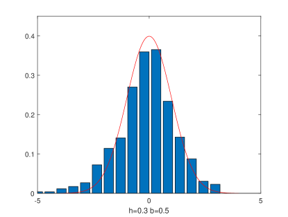
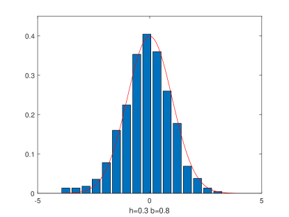
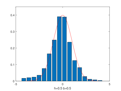
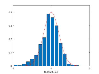
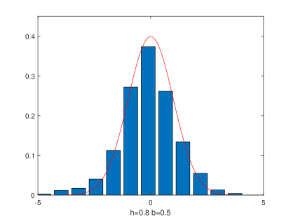
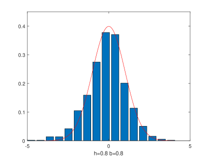
DGP: , where and they are normalized such that , and . The figure plots the histograms of the standardized estimators of the factors using SQR: at from 1000 replications, where is estimated using the formula in Remark 4.4, is the bandwidth parameter in the smoothed check function, and is the bandwidth parameter used in .
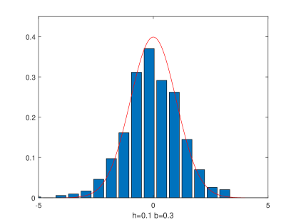
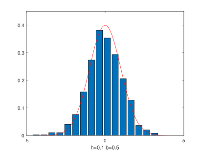
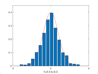
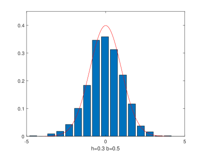
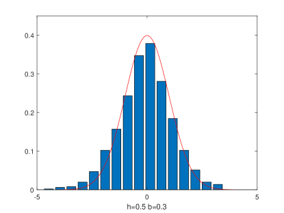
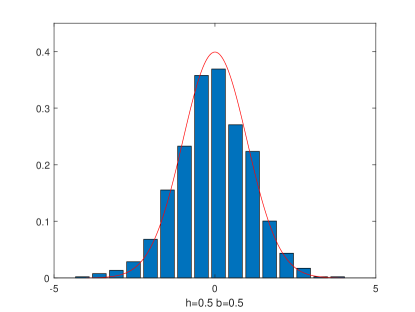
DGP: , where and they are normalized such that , and . The figure plots the histograms of the standardized estimators of the factors using SQR: at from 1000 replications, where is estimated using the formula in Remark 4.4, is the bandwidth parameter in the smoothed check function, and is the bandwidth parameter used in .
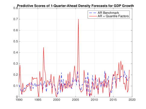
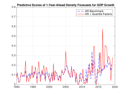
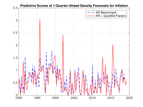
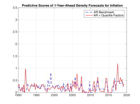
Note: The graphs plot the predictive scores of 1-quarter-ahead and 1-year-ahead density forecasts for real GDP growth and inflation. The evaluation period is from 1990Q1 to 2019Q2, and the out-of-sample forecasting is implemented using rolling windows with 120 observations. The predicted -quantiles are constructed using quantile regressions of the target variable on its owns lags and the estimated quantile factors at (denoted as ). The predicted densities are constructed as the density functions of skewed t-distributions by matching the predicted quantiles of the target variable at . The predictive scores are the predicted densities evaluated at the realized values of the target variable. Higher scores indicate more accurate forecasts. The dotted blue line is the predictive scores of the benchmark AR model where only the lags of the target variable are used to predict the -quantiles, the red line is the predictive scores of the model where is also used to predict the -quantiles.
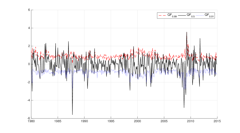
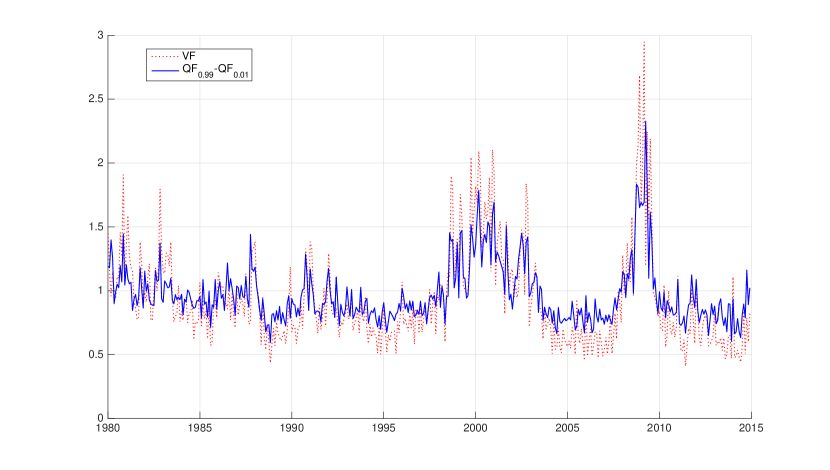
Note: The upper panel presents the QFA factors at and the first QFA factor at from the financial datasets. The lower panel shows the interquantile range (blue line), defined as , alongside the volatility factor (dotted red line) constructed by PCA-SQ. Both series are normalized to have unit length, and their correlation is 0.87.
References
- Adrian et al. (2019) Adrian, T., N. Boyarchenko, and D. Giannone (2019). Vulnerable growth. American Economic Review 109(4), 1263–89.
- Ahn and Horenstein (2013) Ahn, S. C. and A. R. Horenstein (2013). Eigenvalue ratio test for the number of factors. Econometrica 81(3), 1203–1227.
- Amengual and Sentana (2018) Amengual, D. and E. Sentana (2018). Is a normal copula the right copula? Journal of Business & Economic Statistics 0(0), 1–17.
- Andersen et al. (2018) Andersen, T., N. Fusari, and V. Todorov (2018). The pricing of tail risk and the equity premium: Evidence from international option markets. CREATES research papers, Department of Economics and Business Economics, Aarhus University.
- Ando and Bai (2020) Ando, T. and J. Bai (2020). Quantile co-movement in financial markets: A panel quantile model with unobserved heterogeneity. Journal of the American Statistical Association 115(529), 266–279.
- Ang et al. (2006) Ang, A., R. J. Hodrick, Y. Xing, and X. Zhang (2006). The cross-section of volatility and expected returns. The Journal of Finance 61(1), 259–299.
- Angrist et al. (2006) Angrist, J., V. Chernozhukov, and I. Fernández-Val (2006). Quantile regression under misspecification, with an application to the US wage structure. Econometrica 74(2), 539–563.
- Athey and Imbens (2019) Athey, S. and G. W. Imbens (2019). Machine learning methods that economists should know about. Annual Review of Economics 11(1), 685–725.
- Azzalini and Capitanio (2003) Azzalini, A. and A. Capitanio (2003). Distributions generated by perturbation of symmetry with emphasis on a multivariate skew t-distribution. Journal of the Royal Statistical Society: Series B (Statistical Methodology) 65(2), 367–389.
- Bai (2003) Bai, J. (2003). Inferential theory for factor models of large dimensions. Econometrica 71(1), 135–171.
- Bai (2009) Bai, J. (2009). Panel data models with interactive fixed effects. Econometrica 77(4), 1229–1279.
- Bai and Ng (2002) Bai, J. and S. Ng (2002). Determining the number of factors in approximate factor models. Econometrica 70(1), 191–221.
- Bai and Ng (2006) Bai, J. and S. Ng (2006). Confidence intervals for diffusion index forecasts and inference for factor-augmented regressions. Econometrica 74(4), 1133–1150.
- Bai and Ng (2008a) Bai, J. and S. Ng (2008a). Extremum estimation when the predictors are estimated from large panels. Annals of Economics and Finance 9(2), 201–222.
- Bai and Ng (2008b) Bai, J. and S. Ng (2008b). Large dimensional factor analysis. Now Publishers Inc.
- Bai and Ng (2013) Bai, J. and S. Ng (2013). Principal components estimation and identification of static factors. Journal of Econometrics 176(1), 18–29.
- Bai and Ng (2019) Bai, J. and S. Ng (2019). Rank regularized estimation of approximate factor models. Journal of Econometrics 212(1), 78–96.
- Barigozzi and Hallin (2016) Barigozzi, M. and M. Hallin (2016). Generalized dynamic factor models and volatilities: recovering the market volatility shocks. The Econometrics Journal 19(1), 33–63.
- Candès et al. (2011) Candès, E. J., X. Li, Y. Ma, and J. Wright (2011). Robust principal component analysis? Journal of the ACM 58(3), 1–37.
- Chamberlain and Rothschild (1983) Chamberlain, G. and M. Rothschild (1983). Arbitrage, factor structure, and mean-variance analysis on large asset markets. Econometrica 51(5), 1281–304.
- Chen et al. (2017) Chen, L., J. J. Dolado, and J. Gonzalo (2017). Quantile factor models. Working paper, Universidad Carlos III de Madrid.
- Chen et al. (2018) Chen, M., I. Fernández-Val, and M. Weidner (2018). Nonlinear factor models for network and panel data. Working paper, UCL.
- Chen et al. (2009) Chen, X., L. P. Hansen, J. Scheinkman, et al. (2009). Nonlinear principal components and long-run implications of multivariate diffusions. The Annals of Statistics 37(6B), 4279–4312.
- Chudik et al. (2018) Chudik, A., G. Kapetanios, and M. H. Pesaran (2018). A one covariate at a time, multiple testing approach to variable selection in high-dimensional linear regression models. Econometrica 86(4), 1479–1512.
- Collins et al. (2001) Collins, M., S. Dasgupta, and R. E. Schapire (2001). A generalization of principal component analysis to the exponential family. In Proceedings of the 14th International Conference on Neural Information Processing Systems: Natural and Synthetic, NIPS?01, Cambridge, MA, USA, pp. 617?624. MIT Press.
- Connor and Korajczyk (1986) Connor, G. and R. A. Korajczyk (1986). Performance measurement with the arbitrage pricing theory: A new framework for analysis. Journal of Financial Economics 15(3), 373–394.
- de Castro and Galvao (2019) de Castro, L. and A. F. Galvao (2019). Dynamic quantile models of rational behavior. Econometrica 87(6), 1893–1939.
- Forni et al. (2000) Forni, M., M. Hallin, M. Lippi, and L. Reichlin (2000). The generalized dynamic-factor model: Identification and estimation. Review of Economics and statistics 82(4), 540–554.
- Gadea and Gonzalo (2020) Gadea, M. D. and J. Gonzalo (2020). Trends in distributional characteristics: Existence of global warming. Journal of Econometrics 214(1), 153–174.
- Galvao and Kato (2016) Galvao, A. F. and K. Kato (2016). Smoothed quantile regression for panel data. Journal of Econometrics 193(1), 92–112.
- Golub and Van Loan (2013) Golub, G. H. and C. F. Van Loan (2013). Matrix Computations, Volume 3. JHU Press.
- Gorodnichenko and Ng (2017) Gorodnichenko, Y. and S. Ng (2017). Level and volatility factors in macroeconomic data. Journal of Monetary Economics 91, 52–68.
- Hansen et al. (1981) Hansen, J., D. Johnson, A. Lacis, S. Lebedeff, P. Lee, D. Rind, and G. Russell (1981). Climate impact of increasing atmospheric carbon dioxide. Science 213(4511), 957–966.
- Herskovic et al. (2016) Herskovic, B., B. Kelly, H. Lustig, and S. Van Nieuwerburgh (2016). The common factor in idiosyncratic volatility: Quantitative asset pricing implications. Journal of Financial Economics 119(2), 249–283.
- Horowitz (1998) Horowitz, J. (1998). Bootstrap methods for median regression models. Econometrica 66(6), 1327–1352.
- Hotelling (1933) Hotelling, H. (1933). Analysis of a complex of statistical variables into principal components. Journal of Educational Psychology 24(6), 417.
- Hsiang and Kopp (2018) Hsiang, S. and R. E. Kopp (2018). An economist’s guide to climate change science. Journal of Economic Perspectives 32(4), 3–32.
- Koenker (2005) Koenker, R. (2005). Quantile Regression. Number 38. Cambridge University Press.
- Ma et al. (2019) Ma, S., O. Linton, and J. Gao (2019). Estimation and inference in semiparametric quantile factor models. Technical report, Faculty of Economics, University of Cambridge.
- Maravalle and Rawdanowicz (2018) Maravalle, A. and Ł. Rawdanowicz (2018). Changes in economic and financial synchronisation. OECD ECO/WKP 65.
- McCracken and Ng (2016) McCracken, M. W. and S. Ng (2016). FRED-MD: A monthly database for macroeconomic research. Journal of Business & Economic Statistics 34(4), 574–589.
- Muller (1984) Muller, H. G. (1984). Smooth optimum kernel estimators of densities, regression curves and modes. The Annals of Statistics 12(2), 766–774.
- Pelger and Xiong (2018) Pelger, M. and R. Xiong (2018). Interpretable proximate factors for large dimensions. arXiv preprint arXiv:1805.03373.
- Pesaran (2006) Pesaran, M. H. (2006). Estimation and inference in large heterogeneous panels with a multifactor error structure. Econometrica 74(4), 967–1012.
- Powell (1984) Powell, J. L. (1984). Least absolute deviations estimation for the censored regression model. Journal of Econometrics 25(3), 303–325.
- Renault et al. (2017) Renault, E., T. Van Der Heijden, and B. Werker (2017). Arbitrage pricing theory for idiosyncratic variance factors. Working paper, Brown University.
- Ross (1976) Ross, S. A. (1976). The arbitrage theory of capital asset pricing. Journal of Economic Theory 13(3), 341–360.
- Stock and Watson (2002) Stock, J. H. and M. W. Watson (2002). Forecasting using principal components from a large number of predictors. Journal of the American statistical association 97(460), 1167–1179.
- Stock and Watson (2011) Stock, J. H. and M. W. Watson (2011). Dynamic factor models. Oxford Handbook of Economic Forecasting 1, 35–59.
- Su and Wang (2017) Su, L. and X. Wang (2017). On time-varying factor models: Estimation and testing. Journal of Econometrics 198(1), 84–101.
- van de Geer (2002) van de Geer, S. A. (2002). On Hoeffding’s inequality for dependent random variables. In Empirical process techniques for dependent data, pp. 161–169. Springer.
- van der Vaart and Wellner (1996) van der Vaart, A. and J. Wellner (1996). Weak convergence and empirical processes. Springer, New York.
- Vidal et al. (2016) Vidal, R., Y. Ma, and S. Sastry (2016). Generalized Principal Component Analysis, Volume 40. Springer.
- White et al. (2015) White, H., T.-H. Kim, and S. Manganelli (2015). VAR for VaR: Measuring tail dependence using multivariate regression quantiles. Journal of Econometrics 187(1), 169–188.