Sequences of three dimensional manifolds with positive scalar curvature

Abstract.

We develop two new methods of constructing sequences of manifolds with positive scalar curvature that converge in the Gromov-Hausdorff and Intrinsic Flat sense to limit spaces with ”pulled regions”. The examples created rigorously using these methods were announced a few years ago and have influenced the statements of some of Gromov’s conjectures concerning sequences of manifolds with positive scalar curvature. Both methods extend the notion of “sewing along a curve” developed in prior work of the authors with Dodziuk to create limits that are pulled string spaces. The first method allows us to sew any compact set in a fixed initial manifold to create a limit space in which that compact set has been scrunched to a single point. The second method allows us to edit a sequence of regions or curves in a sequence of distinct manifolds.

1. Introduction

In [Gro14], Gromov challenged mathematicians to explore generalized notions of scalar curvature that persist under Gromov-Hausdorff and Intrinsic Flat convergence. The most simply stated geometric definition of scalar curvature at a point,

(1) $${\rm Scal}(p)=\lim_{r\to 0^{+}}30\left(\frac{\operatorname{Vol}_{\mathbb{E}^{3}}(B(0,r))-{\mathcal{H}}^{3}(B(p,r))}{r^{2}\cdot\operatorname{Vol}_{\mathbb{E}^{3}}(B(0,r))}\right),$$

uses Hausdorff measure to replace volume does not behave well under convergence. In joint work of the authors with Dodziuk, we constructed a sequence of manifolds with positive scalar curvature which converged in the Gromov-Hausdorff and Intrinsic Flat sense to a limit space for which this limit is negative at a point [BDS18]. That example was constructed using a method we called “sewing along a curve” and the limit space was a standard three dimensional sphere in which one of the closed geodesics was ”pulled to a point”. In that paper we announced additional examples which we now present here, in which we ”sew” arbitrary compact sets and create limit spaces where the entire compact set is ”pulled to a point”. The examples created here give new insight into the variety of spaces that can appear as limits of manifolds with positive scalar curvature. Indeed the existence of these examples and additional examples by the authors which will appear in upcoming work [BS19], has lead to refinement of Gromov’s conjectures in [Sor17] and new proposed conjectures at the IAS Emerging Topics on Scalar Curvature and Convergence organized by Gromov and the second author in Fall 2018.

The most important theorem concerning manifolds with positive scalar curvature is the Schoen-Yau Positive Mass Theorem [SY79b]. This theorem states that a complete noncompact manifold with positive scalar curvature that is asymptotically flat must have positive ADM mass. The ADM mass is the limit of Hawking masses of increasingly large round spheres in the asymptotically flat region:

(2) $$\mathrm{m}_{\mathrm{ADM}}(M)=\lim_{s\to\infty}\mathrm{m}_{\mathrm{H}}(\Sigma_{s})\in[0,\infty],$$

where the Hawking mass of a surface is defined using the integral of the mean curvature of the surface squared as follows:

(3) $$\mathrm{m}_{\mathrm{H}}(\Sigma)=\frac{1}{2}\left(\frac{A}{\omega_{2}}\right)\left(1-\frac{1}{4\pi}\int_{\Sigma}\left(\frac{H}{2}\right)^{2}\right),$$

Schoen-Yau also prove the rigidity statement that if the ADM mass is zero then the manifold is isometric to Euclidean space. In recent years there has been much work exploring how this theorem is stable under various notions of convergence by the second author and Bamler, Huang, Jauregui, Lee, LeFloch, Mantoulidis, Schoen, Sakovich, Stavrov, and others [Bam16] [LS14][LS15] [HLS16][JL19][SS17][MS14].

In this paper we construct sequences of asymptotically flat manifolds with positive scalar curvature, which converge smoothly outside of a compact set to Euclidean space, but which have various sets within them sewn to points so that the limit space does not satisfy the Schoen-Yau rigidity statement. To construct these sequences we need to develop a second method of sewing manifolds, this time we don’t start with a fixed manifold and creating sewing it more and more tightly, but instead start with a sequence of manifolds and sew each term in the sequence more and more tightly. This is referred to as Method II within.

The paper begins with a review of the notion of a pulled string space first introduced by Burago in discussions with the second author while they were working on ideas leading to [BI09] with Ivanov. Intuitively these spaces are like pieces of cloth in which one string has been pulled tightly, so that it is identified to a point. Here we introduce the idea of a pulled metric space, in which an entire compact set has been pulled to a single point and a method we call scrunching which can be applied to prove a sequence of manifolds converges to a given pulled metric space. This first section is pure metric geometry and does not involve any scalar curvature. It is somewhat technical if one does not already know the methods Gromov-Hausdorff and Intrinsic Flat convergence. A review of the necessary background can be found in [BDS18] so we do not repeat it here.

In Section 2, we introduce our Method I for creating sequences of manifolds with positive scalar curvature that converge to pulled metric spaces. We begin by reviewing the construction of tunnels of positive scalar curvature found by Schoen-Yau [SY79a] and Gromov-Lawson [GL80] (cf the appendix to [BDS18]). We review also the method of sewing along a curve by placing the tunnels in a paired pattern along a fixed curve in a fixed manifold to create a new manifold with positive scalar curvature. One can then sew along the curve more and more tightly, by taking the tunnels smaller and closer together in a precise way, to create a sequence of manifolds with positive scalar curvature that converges to a limit space where that curve has been pulled to a point. All this was done by the authors with Dodziuk in [BDS18]. In our new Method I we extend this to arbitrary compact sets rather than just curves in a fixed Riemannian manifold. This involves the development of a new pattern for placing the tunnels, which is perhaps somewhat similar to a pattern the authors used with Kazaras in [BKS19] except that we are sewing the compact regions tightly to points in this method. In Proposition 3.6 we prove that we obtain a manifold with positive scalar curvature that is sewn. We prove Method I works to produce a pulled limit space in Theorem 3.8.

In Section 3 we apply Method I to present two examples Examples 4.1 and 4.2, although one can easily imagine how it can be applied in many other ways. The limit in Example 4.1 is a standard three dimensional sphere with a single geodesic pulled to a point. The limit in Example 4.2 is a a standard three dimensional sphere with the equatorial sphere pulled to a point. One might in fact create sequences which pull any compact set in a standard three sphere to a point, or indeed any compact set with positive curvature within an arbitrary manifold. It is crucial that the compact set being sewn to a point has small balls isometric to balls in spheres of constant sectional curvature but that constant may be arbitrarily small as long as it is positive (see Proposition 3.6 for the precise requirements).

In Section 4 we develop Method II which provides a method of sewing a sequence of compact sets in a sequence of distinct manifolds. See Theorem 5.1 for the precise statement. Note that this theorem is proven quite generally and does not require positive scalar curvature. It is about when sequences of manifolds created using a scrunching or sewing of regions converges to a certain space. When combined with Proposition 3.6 it can be applied to produce new sequences of manifolds with positive scalar curvature. This method is needed to construct the examples related to the positive mass theorem, because one cannot sew Euclidean space. One can only sew regions with strictly positive sectional curvature. Method II allows us to take sequences of manifolds with positive scalar curvature each with a compact region of positive sectional curvature to produce a Euclidean limit space that has a compact sewn to a point.

In Section 5, we apply Method II to present Examples 6.7-6.9 in which a sequence of asymptotically flat manifolds with positive scalar curvature and ADM mass converging to 0 converge in the pointed Gromov-Hausdorff and intrinsic flat sense to Euclidean Space with a compact set pulled to a point. The construction begins using a sequence of manifolds found in work of the second author with Lee in [LS12] of smooth spherically symmetric manifolds with positive ADM mass converging to 0 that have rings of constant positive sectional curvature. These rings are the compact sets that are sewn so that in the limit the ring is pulled to a point.

Some of this research was completed at the CUNY Graduate Center as part of the the first author’s doctoral dissertation completed under the supervision of Dodziuk and the second author. A few of the examples were announced there, and also in the second author’s survey [Sor17], and have been presented many times. This is the first time the work has been completed rigorously for publication. It should be noted that additional examples constructed using Method II and announced in the first author’s thesis and [Sormani-scalar] concerning limits of almost nonegative scalar curvature will appear rigorously in upcoming work by the authors [BS19]. We would like to thank Jeff Jauregui, Marcus Khuri, Sajjad Lakzian, Dan Lee, Raquel Perales, Conrad Plaut, Catherine Searle, Dan King, and Philip Ording for their interest in this work.

2. Converging to Pulled Metric Spaces

In this paper the limits of our sequences of Riemannian manifolds will no longer be Riemannian manifolds. They will be pulled metric spaces created by taking Riemannian manifold and “pulling a compact set to a point”. We review this notion in the first subsection and then provide a subsection describing a setting when a sequence of Riemannian manifolds converges to such a pulled metric space. Within this second subsection we recall key methods used to prove Gromov-Hausdorff, metric measure, and intrinsic flat convergence as needed. We also recall many lemmas proven in the author’s joint work with Dodziuk [BDS18]. Doctoral students are recommended to read that paper before this one for a thorough review of all the background material.

Note that this section does not involve scalar curvature in any way. It develops the metric geometry required to prove our new examples of sequences of manifolds with scalar curvature bounds converge as we claim they converge. These techniques will be applied elsewhere in the future in upcoming work of the authors.

2.1. Pulled Metric Spaces

A special kind of pulled metric space called a pulled string space was first described to the second author by Dimitri Burago when they were working together on ideas that lead towards an intriguing paper of Burago and Ivanov [Burago-Ivanov-Area]. One starts with a standard square patch of cloth, $X=[0,1]^{2}$, and a string $C:[0,1]\to X$ where $C(t)=(t,1/2)$. One creates the pulled string space

(4) $$Y:=(X\setminus K)\sqcup\{p_{0}\},\qquad p_{0}\in K\,\textrm{fixed},$$

where $K$ is the image of $C$. This pulled string space, $Y$, may intuitively be viewed as the square patch of cloth with a single thread (identified by the curve $C$) which has been pulled tight. Such pulled string spaces starting from an arbitrary geodesic metric space $X$ were described in detail in joint work of the authors with Dodziuk in [BDS18] where we proved the following proposition:

Proposition 2.1.

The notion of a metric space with a pulled string is a metric space $(Y,d_{Y})$ constructed from a metric space $(X,d_{X})$ of Hausdorff dimension $\geq 2$ with a curve $C:[0,1]\to X$, so that

(5) $$Y=X\setminus C[0,1]\sqcup\{p_{0}\},\qquad p_{0}=C(0),$$

where for $x_{i}\in Y$ we have

(6) $$d_{Y}(x,p_{0})=\min\{d_{X}(x,C(t)):\,t\in[0,1]\}$$

and for $x_{i}\in X\setminus C[0,1]$ we have

(7) $$d_{Y}(x_{1},x_{2})=\min\left\{\,d_{X}(x_{1},x_{2}),\min\{d_{X}(x_{1},C(t_{1}))+d_{X}(x_{2},C(t_{2})):\,t_{i}\in[0,1]\}\,\right\}.$$

If $(X,d,T)$ is a Riemannian manifold then $(Y,d,\psi_{\#}T)$ is an integral current space whose mass measure is the Hausdorff measure on $Y$ and

(8) $$\mathcal{H}_{Y}^{m}(Y)=\mathcal{H}_{X}^{m}(X)-\mathcal{H}_{X}^{m}(K).$$

If $(X,d_{X},T)$ is an integral current space then $(Y,d_{Y},\psi_{\#}T)$ is also an integral current space where $\psi:X\to Y$ such that $\psi(x)=x$ for all $x\in X\setminus C[0,1]$ and $\psi(C(t))=p_{0}$ for all $t\in[0,1]$. So that

(9) $${\mathbf{M}}(\psi_{\#}T)={\mathbf{M}}(T)$$

Here we will pull an entire compact set, $K\subset X$, to a point. In our applications, $X$ will be a Riemannian manifold and $K$ a compact submanifold in the Riemannian manifold. This is described here in the following pair of lemmas proven in [BDS18]. Note that it is only called a pulled string space if $K$ is the image of a curve.

Lemma 2.2.

Given a metric space $(X,d_{X})$ and a compact set $K\subset X$ we may define a new metric space $(Y,d_{Y})$ pulling the set $K$ to a point $p_{0}\in K$ by setting

(10) $$Y:=(X\setminus K)\sqcup\{p_{0}\},\qquad p_{0}\in K\,\,\textrm{fixed},$$

and, for $x\in Y$, we have

(11) $$d_{Y}(x,p_{0})=\min\{d_{X}(x,y):\,y\in K\}$$

and, for $x_{i}\in Y\setminus\{p_{0}\}$, we have

(12) $$d_{Y}(x_{1},x_{2})=\min\left\{d_{X}(x_{1},x_{2}),\min\{d_{X}(x_{1},y_{1})+d_{X}(x_{2},y_{2}):\,y_{i}\in K\}\right\}.$$

Lemma 2.3.

If $(X,d_{X},T)$ is an integral current space with a compact subset $K\subset X$ then $(Y,d_{Y},\psi_{\#}T)$ is also an integral current space where $(Y,d_{Y})$ is defined as in Lemma 2.2 and where $\psi:X\to Y$ such that $\psi(x)=x$ for all $x\in X\setminus K$ and $\psi(q)=p_{0}$ for all $q\in K$. In addition

(13) $${\mathbf{M}}(\psi_{\#}T)={\mathbf{M}}(T)-||T||(K)$$

If $(X,d_{X},T)$ is a Riemannian manifold then $(Y,d_{Y},\psi_{\#}T)$ is an integral current space whose mass measure is the Hausdorff measure on $Y$ and

(14) $$\mathcal{H}_{Y}^{m}(Y)=\mathcal{H}_{X}^{m}(X)-\mathcal{H}_{X}^{m}(K).$$

2.2. Scrunching to Pulled Metric Spaces

In this subsection we generalize a theorem proven by the authors with Dodziuk in [BDS18] concerning the limit of a sequence of manifolds which “scrunch” a compact set to a point as follows:

Definition 2.4.

Given a single Riemannian manifold, $M^{3}$, with a compact set, $A_{0}\subset M$. A sequence of manifolds,

(15) $$N_{j}^{3}=(M^{3}\setminus A_{\delta_{j}})\sqcup A^{\prime}_{\delta_{j}}$$

is said to scrunch $A_{0}$ down to a point if $A_{\delta}=T_{\delta}(A_{0})$ and $A^{\prime}_{\delta}$ satisfies:

(16) $$\operatorname{Vol}(A_{\delta}^{\prime})\leq\operatorname{Vol}(A_{\delta})(1+\epsilon)$$

and

(17) $$\operatorname{Vol}(N^{3})\leq\operatorname{Vol}(M^{3})(1+\epsilon)$$

and

(18) $$\operatorname{Diam}(A_{\delta}^{\prime})\leq H$$

where $\epsilon=\epsilon_{j}\to 0$ and where $H=H_{j}\to 0$ and $2\delta_{j}<H_{j}$.

The region $A_{0}^{\prime}$ is referred to as the “edited region” constructed via tunnel surgeries and is explicitly detailed in Section 3 below.

We prove the following new theorem:

Theorem 2.5.

The sequence $N_{j}^{3}$ as in Definition 2.4 where $M^{3}$ is taken to be compact and $A_{0}$ a compact, embedded submanifold of dimension 1 to 3 converges in the Gromov-Hausdorff sense,

(19) $$N_{j}^{3}\stackrel{{\scriptstyle\textrm{GH}}}{{\longrightarrow}}N_{\infty},$$

and the intrinsic flat sense,

(20) $$N_{j}^{3}\stackrel{{\scriptstyle\mathcal{F}}}{{\longrightarrow}}N_{\infty},$$

where $N_{\infty}$ is the metric space created by taking $M^{3}$ and pulling $A_{0}$ to a point $p_{0}$ as in Lemmas 2.2- 2.3.

If, in addition, ${\mathcal{H}}^{3}(A_{0})=0$ then we also have convergence in the metric measure sense

(21) $$N_{j}^{3}\stackrel{{\scriptstyle\textrm{mGH}}}{{\longrightarrow}}N_{\infty}.$$

Note that when $A_{0}$ is the image of a curve, then $N_{\infty}$ is a pulled thread space as in Remark 2.1. In [BDS18], the authors and Dodziuk proved Theorem 2.5 in that special case only with stronger consequences that only hold in that setting.

Within this proof we will state four lemmas proven by the authors with Dodziuk in [BDS18]. We state them because we will apply them again later in the paper. We state them within the proof so that we may motivate and explain them.

Proof.

One first constructs a map $F_{j}:N_{j}\to N_{\infty}$ which is the identity away from the region containing all the tunnels and maps the entire regions containing the tunnels to a single point. More precisely one applies the following lemma from [BDS18]:

Lemma 2.6.

Given $M^{3}$ a compact Riemannian manifold (possibly with boundary) and a smooth embedded compact zero to three dimensional submanifold $A_{0}\subset M^{3}$ (possibly with boundary), and $N_{j}$ as in Definition 2.4. Then for $j$ sufficiently large there exist surjective Lipschitz maps

(22) $$F_{j}:N_{j}^{3}\to N_{\infty}\textrm{ with }\operatorname{Lip}(F_{j})\leq 4$$

where $N_{\infty}$ is the metric space created by taking $M^{3}$ and pulling $A_{0}$ to a point $p_{0}$ as in Lemmas 2.2- 2.3.

In [Gro99], Gromov proved that the Gromov-Hausdorff distance between metric spaces satisfies,

(23) $$d_{GH}(N_{j},N_{\infty})\leq 2H_{j},$$

if there is a map $F_{j}:N_{j}^{3}\to N_{\infty}$ which is an $H_{j}$-almost isometry:

(24) $$|d_{N_{\infty}}(F_{j}(p),F_{j}(q))-d_{N_{j}}(p,q)|\leq H_{j}$$

and

(25) $$\forall y\in N_{\infty}\,\,\,\exists x\in N_{j}\textrm{ such that }d_{N_{\infty}}(F_{\infty}(x),y)\leq H_{j}.$$

The converse is also true requiring again a factor of two: if there is an $H_{j}$-almost isometry then the Gromov-Hausdorff distance between the spaces is $\leq 2H_{j}$. Applying this we have the following lemma proven in [BDS18]:

Lemma 2.7.

Given $N_{j}^{3}$ as in Definition 2.4, the maps $F_{j}:N_{j}^{3}\to N_{\infty}$ of (22) are $H_{j}$-almost isometries with $\lim_{j\to\infty}H_{j}=0$. Thus

(26) $$N_{j}\stackrel{{\scriptstyle\textrm{GH}}}{{\longrightarrow}}N_{\infty}.$$

In order to prove metric measure convergence one needs only to show $F_{j}$ push forward the measures to measures that converge to the measure on the limit space. This only works when $A_{0}$ has measure $0$. One obtains this in the following lemma proven in [BDS18]:

Lemma 2.8.

Given $N_{j}^{3}\to N_{\infty}$ as in Lemma 2.6 endowed with the Hausdorff measures, then we have metric measure convergence if $A_{0}$ has $\mathcal{H}^{3}$-measure $0$.

Whenever one has Gromov-Hausdorff convergence, it was proven by the second author with Wenger in [SW11] that a subsequence converges to an intrinsic flat limit lying within the Gromov-Hausdorff limit. However due to collapse or cancellation the limits might not agree. The intrinsic flat limit is always a rectifiable metric space lying within the Gromov-Hausdorff limit. In order to prove intrinsic flat convergence one may apply a theorem of the second author proven in [Sor14]. This was done to show the following lemma.

Lemma 2.9.

Let $N_{j}^{3}$ be exactly as in Lemma 2.6 and Lemma 2.7 where we assume $M^{3}$ is compact and we have a compact set, $A_{0}\subset M\setminus\partial M$. Then there exists an integral current space $N$ such that $\bar{N}$ is isometric to $N_{\infty}$ and

(27) $$N_{j}\stackrel{{\scriptstyle\mathcal{F}}}{{\longrightarrow}}N_{\infty},[FIXED]$$

where $N_{\infty}$ is given the integral current as in Lemma 2.3, and when $A_{0}$ has $\mathcal{H}^{3}$-measure $0$,

(28) $${\mathbf{M}}(N_{j})\to{\mathbf{M}}(N)=\mathcal{H}^{3}(N).$$

This was proven in [BDS18] in the case when $A_{0}$ was a curve. The only fact that needs to be checked in the present case is that $N=\bar{N}$, or that $p_{0}$ has positive density.

Since

(29) $$\liminf_{r\to 0}\frac{\operatorname{Vol}_{N_{\infty}}(B(p_{0},r))}{r^{3}}=\liminf_{r\to 0}\frac{\operatorname{Vol}_{M}(T_{r}(A_{0})\setminus A_{0})}{r^{3}}$$

Thus $N$ is isometric to $N_{\infty}$ when this liminf is positive and $N$ is isometric to $N_{\infty}\setminus\{p_{0}\}$ when this liminf is $0$. Since $A_{0}$ is a compact, embedded submanifold of dimension $d=1,2,3$ in a 3 dimensional Riemannian manifold we have

(30) $$\liminf_{r\to 0}\frac{\operatorname{Vol}_{M}(T_{r}(A_{0})\setminus A_{0})}{r^{3}}=\liminf_{r\to 0}\frac{\omega_{d}r^{3-d}\cdot{\mathcal{H}}^{d}(A_{0})}{r^{3}}=+\infty>0,$$

since ${\mathcal{H}}^{d}(A_{0})$ is never zero. Thus $N$ is isometric to $N_{\infty}$.

Applying this final lemma the proof of Theorem 2.5 is complete. ∎

2.3. Remarks on Convergence to Pulled Limit Spaces

Sequences of Riemannian manifolds with sectional curvature uniformly bounded below converge in the Gromov-Hausdorff and Intrinsic Flat sense to Alexandrov spaces with curvature bounded below (cf. [BBI01]). It can be seen that a sequence of $N_{j}$ as in Definition 2.4 that also have a uniform lower bound on sectional cannot exist because if they did they would have a limit which is a pulled space that fails to have Alexandrov curvature bounded below.

Noncollapsing sequences of Riemannian manifolds with Ricci curvature uniformly bounded below converge in the Gromov-Hausdorff and Intrinsic Flat sense to spaces whose Hausdorff measure satisfies the appropriate Bishop-Gromov Volume Comparison Theorem. It can be shown that that a noncollapsing sequence of $N_{j}$ as in Definition 2.4 that also have a uniform lower bound on Ricci curvature cannot exist because if they did they would have a limit which is a pulled space whose Hausdorff measure fails to satisfy the Bishop-Gromov Volume Comparison Theorem.

However we can construct sequences of manifolds with positive scalar curvature that converge to a wide variety of interesting pulled limit spaces.

3. Method I: Sewing a Fixed Manifold

This first method takes a fixed Riemannian manifold, $M^{3}$, with positive scalar curvature that has a region with constant positive sectional curvature $K$ about compact set $A_{0}$. We then construct a sequence of Riemannian manifolds, $N_{j}^{3}$, that also have positive scalar curvature that converge to a pulled space constructed from $M^{3}$ by pulling the compact set $A_{0}$ to a point. The process which we call “sewing a region” involves constructing many tunnels between many points in the region.

We break this section into three parts: first we describe a typical tunnel, then we describe how to glue a whole collection of tiny tunnels into a manifold, we do this in a very specific way to sew the region, and finally we prove convergence of the sequence to the pulled limit.

3.1. Tunnels with Positive Scalar Curvature

Using different techniques, Gromov-Lawson and Schoen-Yau described how to construct tunnels diffeomorphic to ${\mathbb{S}}^{2}\times[0,1]$ with metric tensors of positive scalar curvature that can be glued smoothly into three dimensional spheres of constant sectional curvature [GL80][SY79a]. One may imagine constructing such a tunnel by taking the Schwarzschild Riemannian manifold, dropping a tangent sphere from above and raising one from below, and then smoothing in a way such that the scalar curvature becomes positive. See Figure 1. These tunnels are the first crucial piece for our construction.

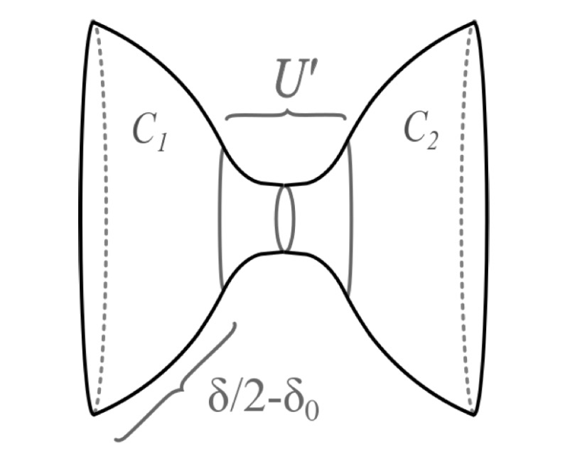
Figure 1. The tunnel $U$.

These tunnels can be made long or short, or arbitrarily tiny. Tiny ones are rigorously constructed by the first author with J. Dodziuk in the appendix to [BDS18]. In their work, the tunnels were used to bridge between two regions within a single manifold where the regions are isometric to convex balls in round three spheres. To be more precise, they have proven Lemma 3.1 which we restate below. Note also Remark 3.3 following the statement.

Lemma 3.1.

Let $0<\delta/2<1$. Given a complete Riemannian manifold, $M^{3}$, that contains two balls $B(p_{i},\delta/2)\subset M^{3}$, $i=1,2$, with constant positive sectional curvature $K\in(0,1]$ on the balls, and given any $\epsilon>0$, there exists a $\delta_{0}>0$ sufficiently small so that we may create a new complete Riemannian manifold, $N^{3}$, in which we remove two balls and glue in a cylindrical region, $U$, between them:

(31) $$N^{3}=M^{3}\setminus\left(B(p_{1},\delta/2)\cup B(p_{2},\delta/2)\right)\sqcup U$$

where $U=U(\delta_{0})$ has a metric of positive scalar curvature with

(32) $$\operatorname{Diam}(U)\leq h=h(\delta),$$

where

(33) $$\lim_{\delta\to 0}h(\delta)=0\textrm{ uniformly for }K\in(0,1].$$

The collars $C_{i}=B(p_{i},\delta/2)\setminus B(p_{i},\delta_{0})$ identified with subsets of $N^{3}$ have the original metric of constant curvature and the tunnel $U^{\prime}=U\setminus(C_{1}\cup C_{2})$ has arbitrarily small diameter $O(\delta_{0})$ and volume $O(\delta_{0}^{3})$. Therefore with appropriate choice of $\delta_{0}$, we have

(34) $$(1-\epsilon)2\operatorname{Vol}(B(p,\delta/2))\leq\operatorname{Vol}(U)\leq(1+\epsilon)2\operatorname{Vol}(B(p,\delta/2))$$

and

(35) $$(1-\epsilon)\operatorname{Vol}(M)\leq\operatorname{Vol}(N)\leq(1+\epsilon)\operatorname{Vol}(M).$$

Remark 3.2.

After inserting the tunnel, $\partial B(p_{1},\delta/2)$ and $\partial B(p_{2},\delta/2)$ are arbitrarily close together because of (33).

Remark 3.3.

We note that since the scalar curvature inside the tunnel is positive we have the following fact applied by the authors and Dodziuk in [BDS18]:

(36) $${\rm Scal}_{p}>0\,\,\forall p\in M\quad\implies\quad{\rm Scal}_{p}>0\,\,\forall p\in N.$$

In this paper we will also apply the fact:

(37) $${\rm Scal}_{p}\geq-\varepsilon\,\,\forall p\in M\quad\implies\quad{\rm Scal}_{p}\geq-\varepsilon\,\,\forall p\in N.$$

3.2. Gluing tunnels into a Fixed Manifold

In [BDS18], the authors and Dodziuk described a process of altering a manifold with positive scalar curvature, $M$, to build a sewn manifold, $N$. This process called sewing along a curve, $C:[0,1]\to M$, involved cutting out a sequence of balls about carefully chosen sequential points, $C(t_{i})$, along the curve and replacing them with tunnels running from the sphere about $C(t_{2i})$ to the sphere about $C(t_{2i+1})$. The first step in the construction was the following proposition which we will apply again in this paper to a completely different collection of points to create our new method of construction:

Proposition 3.4.

Given a complete Riemannian manifold, $M^{3}$, and $A_{0}\subset M^{3}$ a compact subset with an even number of points $p_{i}\in A_{0}$, $i=1,\ldots,n$, with pairwise disjoint contractible balls $B(p_{i},\delta)$ which have constant positive sectional curvature $K$, for some $\delta>0$, define $A_{\delta}=T_{\delta}(A_{0})$ and

(38) $$A_{\delta}^{\prime}=A_{\delta}\setminus\left(\bigcup_{i=1}^{n}B(p_{i},\delta/2)\right)\sqcup\bigcup_{i=1}^{n/2}U_{i}$$

where $U_{i}$ are the tunnels as in Lemma 3.1 connecting $\partial B(p_{2j+1},\delta/2)$ to $\partial B(p_{2j+2},\delta/2)$ for $j=0,1,\ldots,n/2-1$. Then given any $\epsilon>0$, shrinking $\delta$ further, if necessary, we may create a new complete Riemannian manifold, $N^{3}$,

(39) $$N^{3}=(M^{3}\setminus A_{\delta})\sqcup A_{\delta}^{\prime}$$

satisfying

(40) $$(1-\epsilon)\operatorname{Vol}(A_{\delta})\leq\operatorname{Vol}(A_{\delta}^{\prime})\leq\operatorname{Vol}(A_{\delta})(1+\epsilon)$$

and

(41) $$(1-\epsilon)\operatorname{Vol}(M^{3})\leq\operatorname{Vol}(N^{3})\leq\operatorname{Vol}(M^{3})(1+\epsilon).$$

If, in addition, $M^{3}$ has non-negative or positive scalar curvature, then so does $N^{3}$. In fact,

(42) $$\inf_{x\in M^{3}}{\rm Scal}_{x}\geq\min\left\{0,\inf_{x\in N^{3}}{\rm Scal}_{x}\right\}$$

If $\partial M^{3}\neq\emptyset$, the balls avoid the boundary and $\partial M^{3}$ is isometric to $\partial N^{3}$.

Definition 3.5.

We say that we have glued the manifold to itself with a tunnel between the collection of pairs of sphere $\partial B(p_{i},\delta)$ to $\partial B(p_{i+1},\delta)$ for $i=1$ to $n-1$.

3.3. Sewing Compact Sets

Here we introduce the notion of sewing a compact set in a manifold. This is very different from the notion of sewing along a curve that was introduced by the authors with Dodziuk in [BDS18]. In both one constructs a collection of tunnels in the space using Proposition 3.4, however, when one sews along a curve the balls are simply lined up along the curve. To sew a region the picture is much more complicated.

The goal is to scrunch the region to a point as in Definition 2.4. So we need to use the tunnels to bring every point in the region close to any other point in the region. Before stating and proving our proposition we describe the key idea with a figure.

We start with a compact subset $A_{0}$ of $M^{3}$ with a tubular neighborhood that is isometric to a compact subset of a sphere with constant sectional curvature. We cover the tubular neighborhood with $n$ balls of small equal radius, and consider the disjoint collection of balls of radius $r$ about the same points. Every point in the tubular neighborhood is close to one of the $r$-balls.

In every one of the $r$-balls we cut out $(n-1)$ tiny disjoint balls of radius $\delta$. We then glue tunnels between these tiny $\delta$-balls so that there is a tunnel running from any small $r$-ball to any other small $r$-ball using Proposition 3.4. See Figure 2 which has $n=3$ $r$-balls and $n(n-1)=6$ $\delta$-balls and $n(n-1)/2=3$ tunnels.

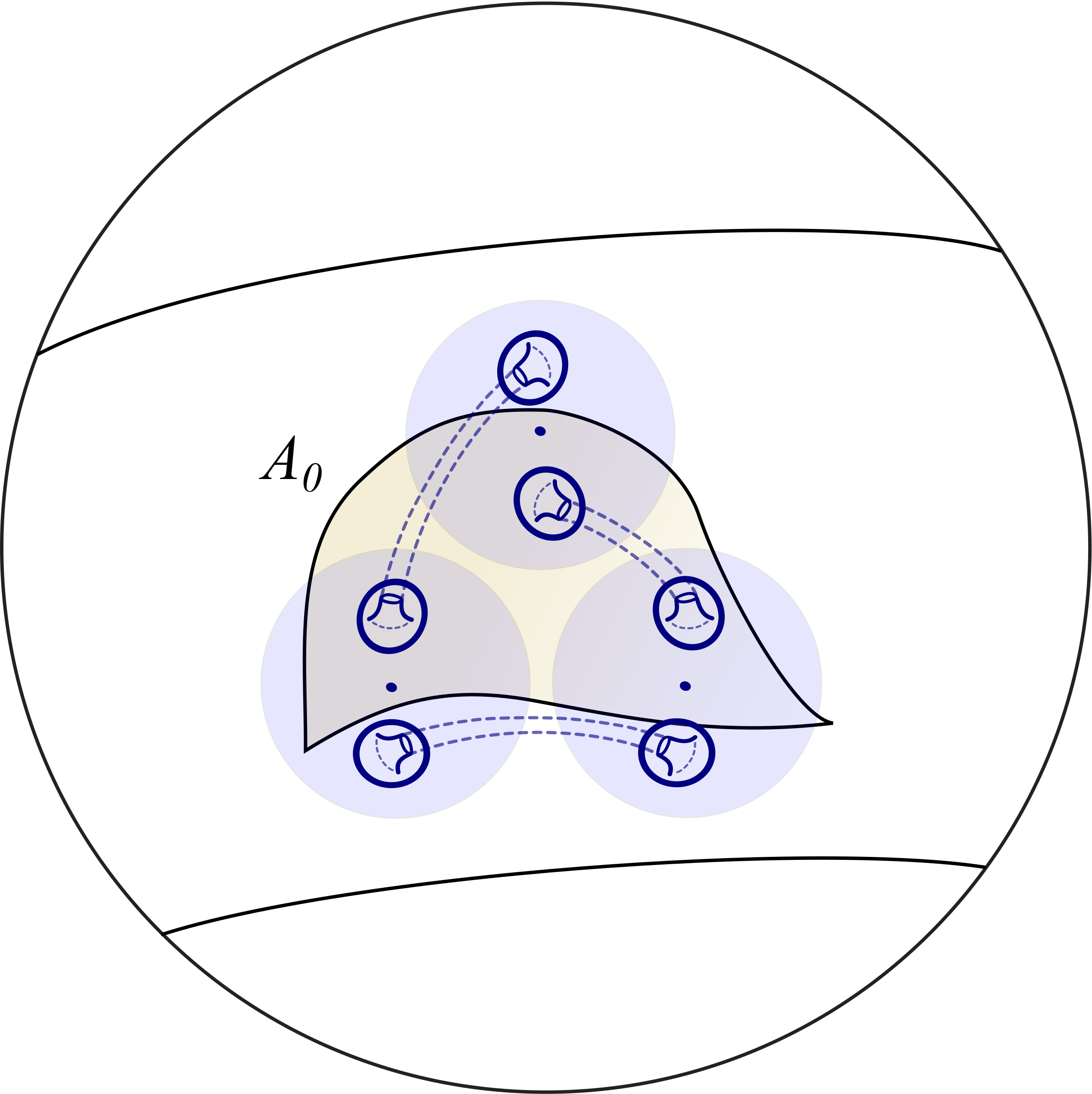
Figure 2. Sewing a manifold through six balls along a region.

Once we have done this sewing we will have created a new sewn manifold $N^{3}$ with $n(n-1)/2$ tunnels. One may think of this $N^{3}$ as being a new version of $M^{3}$ with a collection of star gates, providing quick service from anywhere in the special region $A_{0}$ to anywhere else in the special region. To draw a minimal path from $p$ to $q$, one runs the path through the tunnel between the $r$-ball closest to $p$ and the $r$-ball closest to $q$. Away from the special region $A_{0}$, $N^{3}$ is isometric to $M^{3}$ but it is scrunched on that region.

Proposition 3.6.

Given a complete Riemannian manifold, $M^{3}$, and a compact set $A_{0}\subset M^{3}$ whose tubular neighborhood, $A_{a}=T_{a}(A_{0})$, is Riemannian isometric to a subset of a sphere of constant sectional curvature.

Let $r\in(0,a)$. Given $\epsilon>0$, there exists $\delta=\delta(A_{0},K,r,\epsilon)\in(0,r)$ and there exists even $n=\bar{n}(\bar{n}-1)$ depending on $A_{0},K$, $\epsilon$, and $r$ and points $p_{1},...,p_{n}\in A_{0}$ with $B(p_{i},\delta)$ are pairwise disjoint such that we can “sew the region tightly” to create a new complete Riemannian manifold $N^{3}$,

(43) $$N^{3}=(M^{3}\setminus A_{r})\sqcup A_{r}^{\prime},$$

exactly as in Proposition 3.4, with

(44) $$A_{r}^{\prime}=A_{r}\setminus\left(\bigcup_{i=1}^{n}B(p_{i},\delta/2)\right)\sqcup\bigcup_{i=1}^{n/2}U_{i},$$

so that

(45) $$\operatorname{Vol}(A_{r}^{\prime})\leq\operatorname{Vol}(A_{r})(1+\epsilon)$$

and

(46) $$\operatorname{Vol}(N^{3})\leq\operatorname{Vol}(M^{3})(1+\epsilon)$$

and

(47) $$\operatorname{Diam}(A_{r}^{\prime})\leq H(r,\delta)=16r+3h(\delta).$$

Since $\delta\to 0$ when $r\to 0$,

(48) $$\lim_{r\to 0}H(r,\delta)=0\textrm{ uniformly for }K\in(0,1],$$

we say we have sewn the region $A_{0}$ arbitrarily tightly.

If $M^{3}$ has non-negative or positive scalar curvature, then so does $N^{3}$. In fact,

(49) $$\inf_{x\in M^{3}}{\rm Scal}_{x}\geq\min\left\{0,\inf_{x\in N^{3}}{\rm Scal}_{x}\right\}$$

If $\partial M^{3}\neq\emptyset$, the balls avoid the boundary and $\partial M^{3}$ is isometric to $\partial N^{3}$.

Proof.

Fix $r<a$ as in the proposition statement. For simplicity of notation, let $A=A_{r}$ and $A^{\prime}=A_{r}^{\prime}$.

By the compactness of $A_{0}$ there exists a finite $\bar{n}=\bar{n}(A_{0},r)$ equal to the maximal number of pairwise disjoint balls $\{B(v_{k},r)\}_{k=1}^{\bar{n}}$, centered at $v_{k}\in A_{0}$ of radius $r>0$. Note that $B(v_{k},r)\subset A$.

Let $\delta=\delta(\bar{n},K,r)>0$ be chosen small enough so that for each $k=1$ to $\bar{n}$, there are $\bar{n}-1$ pairwise disjoint balls of radius $\delta$ centered at $v_{kj}$ with $k\neq j$ such that

(50) $$B(v_{kj},\delta)\subset B(v_{k},r)\textrm{ for }j\in\{1,...,\bar{n}\}\setminus\{k\}$$

and each

(51) $$v_{kj}\in\partial B(v_{k},r-\delta).$$

Let

(52) $$n=\bar{n}(\bar{n}-1).$$

We choose the points $p_{i}\in A_{0}$ such that

(53) $$\{p_{1},....,p_{n}\}=\{v_{kj}:\,\,k,j\in\{1,\ldots,\bar{n}\},\,k\neq j\}$$

so that $B(p_{i},\delta)$ are disjoint balls centered in $A_{0}$. In fact we choose $p_{i}$ so that when $i$ is even we have both

(54) $$p_{i}\in\{v_{kj}:\,\,k<j\}$$

and

(55) $$p_{i+1}=v_{jk}\textrm{ iff }p_{i}=v_{kj}$$

and we set

(56) $$U_{kj}=U_{j,k}=U_{i}.$$

We now apply Proposition 3.4 with

(57) $$A^{\prime} = A\setminus\left(\bigcup_{i=1}^{n}B(p_{i},\delta/2)\right)\sqcup\bigcup_{i=1}^{n/2}U_{i}$$

(58) $$= A\setminus\left(\bigcup_{k\neq j}B(v_{kj},\delta/2)\right)\sqcup\bigcup_{k<j}U_{kj}$$

to conclude the volume estimates (45) and (46).

We next verify the diameter estimate of $A^{\prime}$, (47). To do this we define sets $C_{k}\subset A^{\prime}$ which correspond to the sets $\partial B(v_{k},r)\subset A$ which are unchanged because the $B(p_{i},\delta/2)\cap\partial B(v_{k},r)=\emptyset$. We also define sets $C_{kj}\subset A^{\prime}$ which correspond to the sets $\partial B(v_{kj},\delta/2)\subset A$ which are unchanged because they are the edges of the edited regions:

(59) $$C_{kj}\cup C_{jk}=\partial U_{jk}.$$

Let

(60) $$U=\bigcup_{k<j}U_{kj}.$$

Let $x$ and $y$ be arbitrary points in $A^{\prime}$. We first claim there exists $k,j$ such that

(61) $$d_{A^{\prime}}(x,C_{k})<4r+h(\delta)\textrm{ and }d_{A^{\prime}}(y,C_{j})<4r+h(\delta).$$

By symmetry we need only prove this for $x$. Note that in Case I where

(62) $$x\in A^{\prime}\setminus\bigcup_{k<j}U_{kj}=A\setminus\left(\bigcup_{k\neq j}B(v_{kj},\delta/2)\right)$$

then we can view $x$ as a point in $A$. Let $\gamma_{1}\subset A$ be the shortest path from $x$ to the closest point $v_{x}\in A_{0}$, then $L(\gamma_{1})<r$. If

(63) $$\gamma_{1}\cap B(v_{kj},\delta/2)\neq\emptyset$$

then there exists $k$ such that

(64) $$d_{A^{\prime}\setminus U}(x,C_{kj})<\delta$$

and we have

(66) $$d_{A^{\prime}\setminus U}(x,C_{k}) \leq d_{A^{\prime}\setminus U}(x,C_{kj})+\operatorname{Diam}(C_{kj})+d_{A^{\prime}\setminus U}(C_{kj},C_{k})$$

(by the triangle inequality)

(67) $$< r+\operatorname{Diam}(C_{kj})+\delta/2\qquad\textrm{(by (\ref{E:claimdistlessthana}) and (\ref{vkj-edge}))}$$

(68) $$\leq r+\pi(\delta/2)+\delta/2\qquad\textrm{(by sec $\equiv K>0$ on $B(v_{kj},\delta)$)}$$

(69) $$< r+3\delta,$$

so that (61) holds. Otherwise, still in Case I, if (63) fails, $\gamma_{1}\subset A^{\prime}\setminus U$ and $\gamma_{1}(1)=v_{x}\in A_{0}$. Let $\gamma_{2}\subset A$ be the shortest path from $v_{x}$ to the nearest $\partial B(v_{k^{\prime}},r)$. Then $L(\gamma_{2})<r$ because this was a maximal collection of disjoint balls. If

(70) $$\gamma_{2}\cap B(v_{kj},\delta/2)\neq\emptyset$$

then there exists $k$ such that

(71) $$d_{A^{\prime}\setminus U}(v_{x},C_{kj})<r$$

and we have

(73) $$d_{A^{\prime}\setminus U}(v_{x},C_{k}) \leq d_{A^{\prime}\setminus U}(v_{x},C_{kj})+\operatorname{Diam}(C_{kj})+d_{A^{\prime}\setminus U}(C_{kj},C_{k})$$

(by the triangle inequality)

(74) $$< (r-\delta/2)+\operatorname{Diam}(C_{kj})+\delta/2\qquad\textrm{(by (\ref{E:claimdistlessthanr}) and (\ref{vkj-edge}))}$$

(76) $$\leq (r-\delta/2)+\pi(\delta/2)+\delta/2$$

(by sec $$\equiv K>0 B(v_{kj},\delta)$$ on )

(77) $$< r+2\delta$$

so, because $\delta<r$,

(78) $$d_{A^{\prime}\setminus U}(x,C_{k})<L(\gamma_{1})+3r<4r$$

and we have (61). Otherwise, still in Case I but when (70) fails,

(79) $$d_{A^{\prime}\setminus U}(x,C_{k^{\prime}})<L(\gamma_{1})+L(\gamma_{2})<2r.$$

Alternatively, we have Case II where

(80) $$x\in\bigcup_{k<j}U_{kj}.$$

In this case, there exists a $k$ such that $x\in U_{kj}$ and

(81) $$d_{A^{\prime}}(x,C_{k})\leq\operatorname{Diam}(U_{kj})+\operatorname{dist}_{A^{\prime}}(C_{kj},C_{k})\leq h(\delta)+\delta/2<h(\delta)+r.$$

Thus we have the claim in (61).

We now proceed to prove (47) by estimating $d_{A^{\prime}}(x,y)$ for $x,y\in A^{\prime}$. If $j=k$ in (61), then $d_{A^{\prime}}(x,y)\leq 2(4r+h(\delta))$. Otherwise,

(82) $$d_{A^{\prime}}(x,y)\leq 2(4r+h(\delta))+\sup\{d_{A^{\prime}}(z,w)\mid z\in C_{k},w\in C_{j}\}$$

and

(83) $$\sup\{d_{A^{\prime}}(z,w)\mid z\in C_{k},w\in C_{j}\} \leq \operatorname{Diam}_{C_{k}}(C_{k})+\operatorname{dist}(C_{k},C_{kj})+\operatorname{Diam}(U_{kj})$$

$$\qquad+\operatorname{dist}(C_{jk},C_{j})+\operatorname{Diam}(C_{j})$$

(84) $$\leq \pi r+\delta/2+h(\delta)+\delta/2+\pi r$$

(85) $$\leq 8r+h(\delta).$$

Thus, by (82) and (85) we have

(86) $$d_{A^{\prime}}(x,y)\leq 8r+2h(\delta)+8r+h(\delta)\leq 16r+3h(\delta),$$

which is the desired diameter estimate (47).

We observe that by our choice of $\delta$ satisfying $\delta<r$ and the fact that $h(\delta)=O(\delta)$ from Lemma 3.1 we have that (48) holds.

Finally, observe that (49) follows since Lemma 3.1 shows that the tunnels $U_{i}$ have positive scalar curvature. ∎

3.4. Sewing a Fixed Manifold to a Pulled Limit Space

We may now describe our first technique for creating a sequence of manifolds with positive scalar curvature which converge to a pulled metric space. We will start with a fixed Riemannian manifold $M^{3}$ and create an increasingly tightly sewn sequence of manifolds using increasingly dense collections of increasingly tiny balls pairwise connected by increasingly tiny tunnels as in Definition 3.7. We then prove this sequence converges to a pulled metric space in Theorem 3.8.

Definition 3.7.

Given a single compact Riemannian manifold, $M^{3}$, with a compact set, $A_{0}\subset M$, with a tubular neighborhood $A=T_{a}(A_{0})$ which is Riemannian isometric to a tubular neighborhood of a compact set $V\subset\mathbb{S}^{3}_{K}$, in a standard sphere of constant sectional curvature $K$, satisfying the hypothesis of Proposition 3.6. We can construct its sequence of increasingly tightly sewn manifolds, $N_{j}^{3}$, by applying Proposition 3.6 taking $\epsilon=\epsilon_{j}\to 0$, $n=n_{j}\to\infty$, and $\delta=\delta_{j}\to 0$ to create each sewn manifold, $N^{3}=N_{j}^{3}$ and the edited regions $A_{\delta}^{\prime}=A_{\delta_{j}}^{\prime}$ which we simply denote by $A_{j}^{\prime}$. Since these sequences $N_{j}^{3}$ are created using Proposition 3.6, they have nonnegative (resp. positive) scalar curvature whenever $M^{3}$ has nonnegative (resp. positive) scalar curvature and $\partial N_{j}^{3}=\partial M^{3}$ whenever $M^{3}$ has a nonempty boundary.

Note that by Proposition 3.6, the $N_{j}^{3}$ in this sequence are scrunching the compact set $A_{0}$ to a point as in Definition 2.4. Thus our new Theorem 2.5 immediately implies the following theorem:

Theorem 3.8.

The sequence $N_{j}^{3}$, as in Definition 3.7 assuming $M^{3}$ is compactand $A_{0}$ is a compact, embedded submanifold of dimension 1 to 3, converges in the Gromov-Hausdorff sense

(87) $$N_{j}^{3}\stackrel{{\scriptstyle\textrm{GH}}}{{\longrightarrow}}N_{\infty},$$

and the intrinsic flat sense

(88) $$N_{j}^{3}\stackrel{{\scriptstyle\mathcal{F}}}{{\longrightarrow}}N_{\infty},$$

where $N_{\infty}$ is the metric space created by pulling the region $A_{0}\subset M$ to a point as in Lemmas 2.2- 2.3.

If, in addition, ${\mathcal{H}}^{3}(A_{0})=0$ then we also have convergence in the metric measure sense

(89) $$N_{j}^{3}\stackrel{{\scriptstyle\textrm{mGH}}}{{\longrightarrow}}N_{\infty}.$$

A special case of this theorem appeared in [BDS18] where the authors proved that a sequence of manifolds sewn increasingly tightly along the image of a curve converged to a pulled string space.

4. Sewn Spheres and Limits of Volumes

In this section we apply Method I to a standard sphere $M^{3}=\mathbb{S}^{3}$ of constant curvature one with $A_{0}$ chosen to be either a closed geodesic or an equatorial 2-sphere.

The first example appeared in work of the authors with Dodziuk proven by sewing along a curve [BDS18].

Example 4.1.

[BDS18] Let $N_{j}^{3}$ be the sequence of manifolds with positive scalar curvature constructed from the standard sphere, $\mathbb{S}^{3}$, by sewing along a closed geodesic $C:[0,1]\to\mathbb{S}^{3}$ with $\delta=\delta_{j}\to 0$. Then

(90) $$N_{j}^{3}\stackrel{{\scriptstyle\textrm{mGH}}}{{\longrightarrow}}N_{\infty}\textrm{ and }N_{j}^{3}\stackrel{{\scriptstyle\mathcal{F}}}{{\longrightarrow}}N_{\infty}$$

where $N_{\infty}$ is the metric space created by taking the standard sphere and pulling the geodesic to a point as in Proposition 2.1.

Moreover, at the pulled point $p_{0}\in N_{\infty}$ we have $w{\rm Scal}(p_{0})=-\infty$ where $w{\rm Scal}$ is as in (1), i.e.

(91) $$w{\rm Scal}(p_{0})=\lim_{r\to 0^{+}}30\left(\frac{\operatorname{Vol}_{\mathbb{E}^{3}}(B(0,r))-{\mathcal{H}}^{3}(B(p,r))}{r^{2}\cdot\operatorname{Vol}_{\mathbb{E}^{3}}(B(0,r))}\right)=-\infty.$$

This example is depicted in Figure 3.

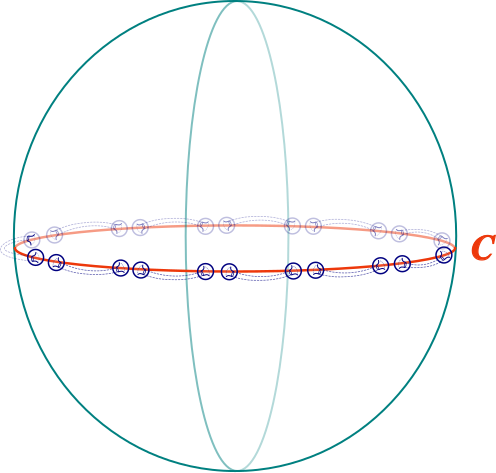
Figure 3. Sewing along a closed geodesic in a sphere $\mathbb{S}^{3}$.

Similarly, when scrunching a 2-sphere inside $\mathbb{S}^{3}$:

Example 4.2.

Let $N_{j}^{3}$ be the sequence of manifolds with positive scalar curvature constructed from the standard sphere, $\mathbb{S}^{3}$, by sewing along an equatorial 2-sphere, $A_{0}=\mathbb{S}_{e}^{2}\subset\mathbb{S}^{3}$, with $\delta=\delta_{j}\to 0$ as in Proposition 3.6. Then

(92) $$N_{j}^{3}\stackrel{{\scriptstyle\textrm{mGH}}}{{\longrightarrow}}N_{\infty}\textrm{ and }N_{j}^{3}\stackrel{{\scriptstyle\mathcal{F}}}{{\longrightarrow}}N_{\infty}$$

where $N_{\infty}$ is the integral current space created by taking the standard sphere and pulling the equatorial sphere to a point as in Lemma 2.2.

Moreover, at the pulled point $p_{0}\in N_{\infty}$ we have $w{\rm Scal}(p_{0})=-\infty$ where $w{\rm Scal}$ is as in (1), i.e.

(93) $$w{\rm Scal}(p_{0})=\lim_{r\to 0^{+}}30\left(\frac{\operatorname{Vol}_{\mathbb{E}^{3}}(B(0,r))-{\mathcal{H}}^{3}(B(p,r))}{r^{2}\cdot\operatorname{Vol}_{\mathbb{E}^{3}}(B(0,r))}\right)=-\infty.$$

Proof.

First, observe that

(94) $$\operatorname{Vol}_{N_{\infty}}(B(p_{0},r)) = \mathcal{H}_{N_{\infty}}^{3}(B(p_{0},r))$$

(95) $$= \mathcal{H}_{N_{\infty}}^{3}(B(p_{0},r)\setminus\{p_{0}\})$$

(96) $$= \mathcal{H}_{\mathbb{S}^{3}}^{3}(T_{r}(\mathbb{S}_{e}^{2})).$$

Since $\mathbb{S}_{e}^{2}$ is a closed equatorial sphere of area $4\pi$ in a three dimensional sphere, we have

(97) $$\lim_{r\to 0}\frac{\mathcal{H}_{\mathbb{S}^{3}}^{3}(T_{r}(\mathbb{S}_{e}^{2}))}{4\pi(2r)}=1.$$

Thus

(98) $$\lim_{r\to 0}\frac{\operatorname{Vol}_{\mathbb{E}^{3}}(B(0,r))-\operatorname{Vol}_{N_{\infty}}(B(p_{0},r))}{r^{2}\operatorname{Vol}_{\mathbb{E}^{3}}(B(0,r))}=\lim_{r\to 0}\frac{(4/3)\pi r^{3}-4\pi(2r)}{(4/3)\pi r^{5}}=-\infty$$

as claimed. ∎

5. Method II: Sewing a Sequence of Manifolds

In order to prove the examples Section 6 and our upcoming paper [BS-tori] we need to develop a more general technique than Method I. Here we start with a converging sequence of Riemannian manifolds with a Riemannian limit and sew regions in that sequence to create a new sequence of Riemannian manifolds with a pulled limit. More precisely, we consider a sequence of smooth Riemanninan manifolds $\{M_{j}^{3}\}_{j\in\mathbb{N}}$ converging in the biLipschitz sense to $M_{\infty}^{3}$ (also a smooth manifold) and, for each manifold $M_{j}^{3}$, construct its sequence of increasingly tightly sewn manifolds $\{N_{j,i}^{3}\}_{i\in\mathbb{N}}$ scrunching a region $A_{j,0}$. Then the following Theorem states, under suitable hypotheses, that a sequence of sewn manifolds $\{N_{j}^{3}\}$ created from $\{N_{j,i}^{3}\}$ converges in the Gromov-Hausdorff and Intrinsic-Flat sense to $N_{\infty}$ which is a pulled space created by scrunching the region $A_{\infty,0}\subset M_{\infty}^{3}$ to a point.

Theorem 5.1.

Given a sequence of compact $M_{j}^{3}$ each with a compact region $A_{j,0}\subset M_{j}^{3}$ with a tubular neighborhood, $A_{j}$, of constant sectional curvature satisfying the hypotheses of Proposition 3.6. We assume $M_{j}^{3}$ converge in the biLipschitz sense to $M_{\infty}^{3}$ and the regions $A_{j,0}$ converge to compact set $A_{\infty,0}\subset M_{\infty}^{3}$ in the sense that there exists biLipschitz maps

(99) $$\psi_{j}:M_{j}^{3}\to M_{\infty}^{3}$$

such that

(100) $$L_{j}=\log\operatorname{Lip}(\psi_{j})+\log\operatorname{Lip}(\psi_{j}^{-1})\to 0$$

and

(101) $$\psi_{j}(A_{j,0})=A_{\infty,0}.$$

Then there exists $\delta_{j}\to 0$ and, applying Proposition 3.6 to $M^{3}=M_{j}^{3}$ to sew the regions $A_{0}=A_{j,0}$ with $\delta=\delta_{j}$, to obtain sewn manifolds $N^{3}=N_{j}^{3}$, we obtain a sequence $N_{j}^{3}$ such that

(102) $$N_{j}^{3}\stackrel{{\scriptstyle\textrm{GH}}}{{\longrightarrow}}N_{\infty}$$

and

(103) $$N_{j}^{3}\stackrel{{\scriptstyle\mathcal{F}}}{{\longrightarrow}}N_{\infty,0}$$

where $\overline{N}_{\infty,0}=N_{\infty}$ and $N_{\infty}$ is the metric space created by taking $M_{\infty}^{3}$ and pulling the region $A_{\infty,0}$ to a point as in Lemma 2.2–Lemma 2.3.

If, in addition, the regions $A_{j,0}$ satisfy $\mathcal{H}^{3}(A_{j,0})=0$, then the sequence $N_{j}^{3}$ also converges in the the metric measure sense

(104) $$N_{j}^{3}\stackrel{{\scriptstyle\textrm{mGH}}}{{\longrightarrow}}N_{\infty}.$$

Proof.

For each $M_{j}^{3}$ in the sequence we can apply Proposition 3.6 to create its increasingly tightly sewn sequence $N_{j,i}^{3}$ with $\lim_{i\to\infty}\delta_{j,i}=0$. By Theorem 3.8, we know that

(105) $$N_{j,i}\stackrel{{\scriptstyle\textrm{GH}}}{{\longrightarrow}}N_{j,\infty}\textrm{ as }i\to\infty$$

and

(106) $$N_{j,i}\stackrel{{\scriptstyle\mathcal{F}}}{{\longrightarrow}}N_{j,0}\textrm{ as }i\to\infty$$

where $N_{j,0}$ is an integral current space satisfying $\bar{N}_{j,0}=N_{j,\infty}$ and $N_{j,\infty}$ is the metric space created by taking $M_{j}^{3}$ and pulling the region $A_{j,0}$ to a point as in Lemma 2.2. For each $j$ take $i_{j}$ sufficiently large that

(107) $$\delta_{i,j}<1/j\qquad\forall i\geq i_{j}$$

(108) $$d_{GH}(N_{j,i},N_{j,\infty})<1/j\qquad\forall i\geq i_{j}$$

and

(109) $$d_{\mathcal{F}}(N_{j,i},N_{j,0})<1/j\qquad\forall i\geq i_{j}$$

and, in the cases we have metric measure convergence,

(110) $$|{\mathbf{M}}(N_{j,i})-{\mathbf{M}}(N_{j,0})|<1/j.$$

We choose $\delta_{j}=\delta_{j,i_{j}}$ and take $N_{j}^{3}=N_{j,i_{j}}^{3}$.

By the triangle inequality we need only prove:

(111) $$d_{GH}(N_{j,\infty},N_{\infty})\to 0$$

and

(112) $$d_{\mathcal{F}}(N_{j,0},N_{\infty,0})\to 0$$

and, in the cases we have measure convergence,

(113) $${\mathbf{M}}(N_{j,0})\to{\mathbf{M}}(N_{\infty}).$$

where $N_{\infty}$ is the metric space created by taking $M_{\infty}^{3}$ and pulling the region $A_{\infty,0}$ to a point as in Lemma 2.2.

Observe that there are 1-Lipschitz maps

(114) $$P_{j}:M_{j}\to N_{j,\infty}\quad\text{and}\quad P_{\infty}:M_{\infty}\to N_{\infty}$$

defined by

(115) $$P_{j}(x)=\begin{cases}p_{j,0}\qquad&\forall\,x\in A_{j,0}\\ x\qquad&\forall\,x\notin A_{j,0}\end{cases}\quad\text{and}\quad P_{\infty}(x)=\begin{cases}p_{\infty,0}\qquad&\forall\,x\in A_{\infty,0}\\ x\qquad&\forall\,x\notin A_{\infty,0}.\end{cases}$$

Next, define invertible maps

(116) $$\bar{\psi}_{j}:N_{j,\infty}\to N_{\infty}\quad\text{and}\quad\bar{\psi}_{j}^{-1}:N_{\infty}\to N_{j,\infty}$$

by

(117) $$\bar{\psi}_{j}(x)=P_{\infty}(\psi_{j}(x))\quad\text{and}\quad\bar{\psi}_{j}^{-1}(y)=P_{j}(\psi_{j}^{-1}(y))$$

Note that (101) implies these are well-defined.

Let $x_{1},x_{2}\in N_{j,\infty}$, then recall that by definition of the distance $d_{N_{j,\infty}}$ in (10)-(12), we have three cases. To simplify notation we shall suppress the $P_{j}$ and $P_{\infty}$ from below.

In Case I, assume that

(118) $$d_{N_{j,\infty}}(x_{1},x_{2})=d_{M_{j}}(x_{1},x_{2})$$

so $x_{1},x_{2}\notin A_{j,0}$. By (116)-(117) and using that $\psi_{j}$ is Lipschitz we have

$$d_{N_{\infty}}(\bar{\psi}_{j}(x_{1}),\bar{\psi}_{j}(x_{2})) \leq d_{M_{\infty}}(\psi_{j}(x_{1}),\psi_{j}(x_{2}))$$

$$\leq\operatorname{Lip}(\psi_{j})d_{M_{j}}(x_{1},x_{2})$$

$$=\operatorname{Lip}(\psi_{j})d_{N_{j,\infty}}(x_{1},x_{2})$$

so that $\operatorname{Lip}(\bar{\psi}_{j})\leq\operatorname{Lip}(\psi_{j})$.

In Case II, assume that

(119) $$d_{N_{j,\infty}}(x_{1},x_{2})=d_{M_{j}}(x_{1},A_{j,0})+d_{M_{j}}(x_{2},A_{j,0})$$

with $x_{1},x_{2}\notin A_{j,0}$. By (116)-(117) and using that $\psi_{j}$ is Lipschitz we have

$$d_{N_{\infty}}(\bar{\psi}_{j}(x_{1}),\bar{\psi}_{j}(x_{2})) \leq d_{M_{\infty}}(\psi_{j}(x_{1}),A_{\infty,0})+d_{M_{\infty}}(\psi_{j}(x_{2}),A_{\infty,0})\qquad\text{($\triangle$ ineq.)}$$

$$\leq\operatorname{Lip}(\psi_{j})\left(d_{M_{j}}(x_{1},A_{j,0})+d_{M_{j}}(x_{2},A_{j,0})\right)$$

$$=\operatorname{Lip}(\psi_{j})d_{N_{j,\infty}}(x_{1},x_{2})$$

so that $\operatorname{Lip}(\bar{\psi}_{j})\leq\operatorname{Lip}(\psi_{j})$.

Finally, in Case III, assume that $x_{2}=p_{j,0}$ and

(120) $$d_{N_{j,\infty}}(x_{1},p_{j,0})=d_{M_{j}}(x_{1},A_{j,0})$$

with $x_{1}\neq p_{j,0}$, or $x_{1}\notin A_{j,0}$. Then since $\bar{\psi}_{j}(x_{2})=p_{\infty,0}$ and using that $\psi_{j}$ is Lipschitz we have

$$d_{N_{\infty}}(\bar{\psi}_{j}(x_{1}),\bar{\psi}_{j}(x_{2})) =d_{N_{\infty}}(\bar{\psi}_{j}(x_{1}),p_{\infty,0})=d_{M_{\infty}}(\psi_{j}(x_{1}),A_{\infty,0})$$

$$\leq\operatorname{Lip}(\psi_{j})d_{M_{j}}(x_{1},A_{j,0})$$

$$=\operatorname{Lip}(\psi_{j})d_{N_{j,\infty}}(x_{1},p_{j,0})$$

so that $\operatorname{Lip}(\bar{\psi}_{j})\leq\operatorname{Lip}(\psi_{j})$.

Thus, in all three cases we have shown that $\bar{\psi}_{j}$ is Lipschitz with $\operatorname{Lip}(\bar{\psi}_{j})\leq\operatorname{Lip}(\psi_{j})$. One can similarly verify that $\bar{\psi}_{j}^{-1}$ is Lipschitz with $\operatorname{Lip}(\bar{\psi}_{j}^{-1})\leq\operatorname{Lip}(\psi_{j}^{-1})$.

So,

(121) $$\bar{L}_{j}=\log\operatorname{Lip}(\bar{\psi}_{j})+\log\operatorname{Lip}(\bar{\psi}_{j}^{-1})\leq L_{j}\to 0$$

by (100).

Thus $N_{j,\infty}$ converges to $N_{\infty}$ in the Lipschitz sense. Since Lipschitz convergence implies Gromov-Hausdorff convergence [Gro99] we have

(122) $$N_{j,\infty}\stackrel{{\scriptstyle\textrm{GH}}}{{\longrightarrow}}N_{\infty}.$$

Moreover, we have Intrinsic Flat convergence,

(123) $$N_{j,\infty}\stackrel{{\scriptstyle\mathcal{F}}}{{\longrightarrow}}N_{\infty,0},$$

by Theorem 5.6 of Sormani–Wenger [SW11] where $N_{\infty,0}\subset N_{\infty}$ with $\bar{N}_{\infty,0}=N_{\infty}$.

To finish, observe that the statement about metric measure convergence now follows from Lemma 2.8. ∎

6. Sequences with ADM mass to 0

We apply the results of the previous Section 5 together with to the examples of the second author with Lee [LS14] to construct new examples of sequences of asymptotically flat manifolds with ADM mass decreasing to zero which converge in the (pointed) Intrinsic Flat- and Gromov-Hausdorff-sense to a (weak) limit that is not the standard flat Euclidean space.

6.1. Sequences with Stripes of Constant Curvature

We review the construction of rotationally symmetric manifolds with nonnegative scalar curvature and small ADM mass following [LS14].

Definition 6.1.

Let $\operatorname{RotSym}_{3}$ be the class of complete $3$-dimensional $SO(3)$-rotationally symmetric smooth Riemannian manifolds of nonnegative scalar curvature which have no closed interior minimal hypersurfaces and either have no boundary or have a boundary which is a stable minimal hypersurface.

Here one can find simple formulas relating Hawking mass and scalar curvature, and observe that Hawking mass is increasing to the ADM mass. In fact one has an embedding into Euclidean space:

Lemma 6.2.

([LS14]) Given $(M^{3},g)\in\operatorname{RotSym}_{3}$, we can find a rotationally symmetric Riemannian isometric embedding of $M^{3}$ into Euclidean space as the graph of some radial function $z=z(r)$ satisfying $z^{\prime}(r)\geq 0$. In graphical coordinates, we have

(124) $$g=(1+[z^{\prime}(r)]^{2})dr^{2}+r^{2}g_{0},$$

with $r\geq r_{min}$ and the following formulae for scalar curvature, area, mean curvature, Hawking mass and its derivative in terms of the radial coordinate $r$:

(125) $$\mathrm{R}(r) =\frac{2}{1+(z^{\prime})^{2}}\left(\frac{z^{\prime}}{r}\right)\left(\frac{z^{\prime}}{r}+\frac{2z^{\prime\prime}}{1+(z^{\prime})^{2}}\right)$$

(126) $$A(r) =\omega_{2}r^{2}$$

(127) $$H(r) =\frac{2}{r\sqrt{1+(z^{\prime})^{2}}}$$

(128) $$\mathrm{m}_{\mathrm{H}}(r) =\frac{r}{2}\left(\frac{(z^{\prime})^{2}}{1+(z^{\prime})^{2}}\right)$$

(129) $$\mathrm{m}_{\mathrm{H}}^{\prime}(r) =\frac{r^{2}}{4}\mathrm{R}$$

This Riemannian isometric embedding is unique up to a choice of $z_{min}=z(r_{min})$.

Lemma 6.3.

([LS14]) There is a bijection between elements of $\operatorname{RotSym}_{3}$ and increasing functions $\mathrm{m}_{\mathrm{H}}:[r_{\textrm{min}},\infty)\to\mathbb{R}$ such that

(130) $$\mathrm{m}_{\mathrm{H}}(r_{\textrm{min}})=\frac{1}{2}r_{\textrm{min}}$$

and

(131) $$\mathrm{m}_{\mathrm{H}}(r)<\frac{1}{2}r$$

for $r>r_{\textrm{min}}\geq 0$. In this section we will call these functions admissible Hawking mass functions.

Given an admissible Hawking function, the function $z:[0,\infty)\to\mathbb{R}$ defined via the formula

(132) $$z(\bar{r})=\int_{r_{\textrm{min}}}^{\bar{r}}\sqrt{\frac{2\mathrm{m}_{\mathrm{H}}(r)}{r-2\mathrm{m}_{\mathrm{H}}(r)}}\,dr$$

determines a rotationally symmetric manifold in $\operatorname{RotSym}_{3}$.

In particular taking a constant Hawking mass, $m_{H}(r)=m_{0}$, we have

(133) $$z(r)=\sqrt{8m_{0}\left(r-2m_{0}\right)},\quad r\in[2m_{0},\infty)$$

with metric

(134) $$g=\left(1+\frac{2m_{0}}{r-2m_{0}}\right)dr^{2}+r^{2}g_{0},$$

which is half of the Riemannian Schwarzschild space. Notice these examples are scalar flat since $\mathrm{R}=0$ by (129).

In order to allow for sewing, we need a region with positive scalar curvature. The second author and Lee show that one can create “stripes” of constant curvature $K>0$ within the class $\operatorname{RotSym}_{3}$ using admissible Hawking functions:

Lemma 6.4.

([LS14]) A manifold $M^{3}\in\operatorname{RotSym}_{3}$ has constant sectional curvature, $K>0$, on $r^{-1}(a,b)$, for $r_{\textrm{min}}<a<b$, iff $r^{-1}(a,b)$ is an annulus in a sphere of radius $1/K^{1/2}$ iff $\mathrm{m}_{\mathrm{H}}(r)=r^{3}K/2$ for $r\in(a,b)$.

See Figure 4.

Figure 4. An asymptotically flat manifold with a stripe of positive scalar curvature whose ADM mass is small.

We will need one final lemma from [LS14]:

Lemma 6.5.

([LS14]) Fix $\alpha>0$. Given any increasing sequence,

(135) $$\{r_{1},r_{2},...\}\subset[\mathrm{m}_{\mathrm{fix}}/2,\infty),$$

there exists $M^{3}\in\operatorname{RotSym}_{3}$ with constant sectional curvature on stripes $r^{-1}(a_{i},b_{i})$ where $(a_{i},b_{i})\subset[r_{2i-1},r_{2i}]$ and $\mathrm{m}_{\mathrm{ADM}}(M)<\alpha$ and $\partial M=\emptyset$.

Based on Lemma 6.5, the second author and Lee constructed examples of a sequence of asymptotically flat manifolds with $ADM$ mass decreasing to zero with an increasing number of long wells that converged in the pointed Intrinsic Flat sense to euclidean space but have no Lipschitz or Gromov-Haudroff converging subsequences:

Example 6.6.

([LS14]) There exists a sequence of asymptotically flat manifolds $M_{i}^{3}$ with no interior minimal surfaces and empty boundary and $\lim_{i\to\infty}\mathrm{m}_{\mathrm{ADM}}(M_{i}^{3})=0$ such that for any $\alpha_{0},D>0$ the sequence of regions $T_{D}(\Sigma)\subset M_{i}^{3}$ where $\operatorname{Vol}_{2}(\Sigma)=\alpha_{0}$ converge in the intrinsic flat sense to $T_{D}(\Sigma)\subset\mathbb{E}^{3}$ but do not even have Lipschitz or Gromov-Hausdorff converging subsequences.

6.2. Failing Almost Rigidity of the Positive Mass Theorem

In this section we apply the sewing technique to sequences of asymptotically flat manifolds with $ADM$ mass decreasing to zero to give new examples which converge (by Theorem 5.1) in the pointed Gromov-Hausdorff and pointed Intrinsic Flat sense to weak limits that are not the standard flat euclidean space.

To complete our constructions, we need a region of constant positive sectional curvature to sew, we use Lemma 6.4. See Figure 4 .

Unlike the sequence of Lee and Sormani, the sequence in Example 6.7 converges in pointed Gromov-Hausdorff sense.

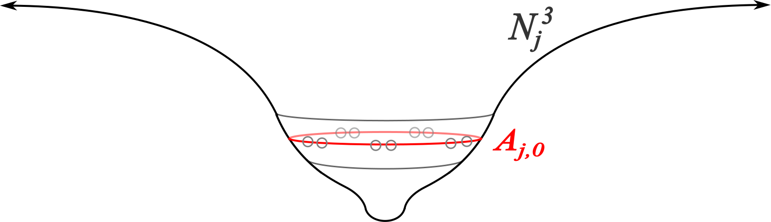
Figure 5. An element of the sequence of asymptotically flat sewn manifolds constructed in Example 6.7.

Example 6.7.

There exists a sequence of asymptotically flat manifolds $N_{j}^{3}$ with nonnegative scalar curvature, empty boundary and $\lim_{j\to\infty}\mathrm{m}_{\mathrm{ADM}}(M_{j}^{3})=0$ that converges in the pointed Gromov-Hausdorff and pointed Intrinsic Flat sense to $\mathbb{E}^{3}$ with a closed curve pulled to a point $p_{0}$ in the following sense: given any $\alpha_{0}>0$ and $D>0$,

(136) $$d_{GH}(T_{D}(\Sigma_{\alpha_{0}})\subset N_{j}^{3},T_{D}(\Sigma_{\alpha_{0}})\subset N_{\infty})\to 0$$

and

(137) $$d_{{\mathcal{F}}}(T_{D}(\Sigma_{\alpha_{0}})\subset N_{j}^{3},T_{D}(\Sigma_{\alpha_{0}})\subset N_{\infty})\to 0$$

where $N_{\infty}$ which is $\mathbb{E}^{3}$ with a closed curve pulled to a point $p_{0}$ as in Lemma 2.2 and $\Sigma_{\alpha_{0}}$ is the surface with $\operatorname{Vol}_{2}(\Sigma_{\alpha_{0}})=\alpha_{0}$. Thus, $N_{\infty}$ is homeomorphic to $\mathbb{E}^{3}\sqcup_{p_{0}}\mathbb{S}^{3}$, which is a wrinkled $\mathbb{E}^{3}$ with a wrinkled sphere attached. See Figure 5.

Proof.

Let $\alpha_{0},D>0$ be given. Set

(138) $$r_{0}=\left(\frac{\alpha_{0}}{4\pi}\right)^{1/2}\qquad\text{and}\qquad r_{1}=\begin{cases}r_{0}-D/2,\quad&r_{0}-D\geq 0\\ r_{0}/2,&\text{otherwise}\end{cases}$$

Fix $j\in\mathbb{N}$. Let $\delta_{j}=1/j$,

(139) $$r_{j,2}=r_{1}-1/j\qquad\text{and }\qquad r_{j,3}=r_{1}+1/j.$$

By Lemma 6.5, there exists rotationally symmetric manifolds $\bar{M}_{j}^{3}\in\operatorname{RotSym}_{3}$ with $\textrm{m}_{\textrm{ADM}}(\bar{M}_{j}^{3})<\delta_{j}$ and with constant sectional curvature $K_{j}>0$ on the stripe

(140) $$r^{-1}(a_{j},b_{j})\subset r^{-1}[r_{j,2},r_{j,3}],$$

for some $a_{j}<b_{j}$ in the interval $[r_{j,2},r_{j,3}]$.

Let $M_{j}^{3}=Cl(T_{D}(\Sigma_{j,0}))\subset\bar{M}_{j}^{3}$ and $M_{\infty}^{3}=Cl(T_{D}(\Sigma_{0}))\subset\mathbb{E}^{3}$, where $\Sigma_{j,0}$ and $\Sigma_{0}$ are the surfaces with area equal to $\alpha_{0}$ and, thus, are at a distance of $r_{0}$ from the axis (in graphical coordinates). Further, let $A_{j,0}$ be closed geodesic circle inside $r^{-1}((a_{j}+b_{j})/2)$ in $M_{j}^{3}$. Let $A_{\infty,0}$ be the circle centered at $0$ in $\mathbb{E}^{3}$ of radius $r_{1}$. Observe that by our choices in (138) and (139) the stripe of constant sectional curvature $r^{-1}(a_{j},b_{j})$ always belongs to $M_{j}$ (including $j=\infty)$.

The tubular neighborhoods $M_{j}^{3}$ and $M_{\infty}^{3}$ are isometrically embedded into $\mathbb{E}^{4}$ by Lemma 6.2, so there exist biLipschitz maps $\psi_{j}:M_{j}^{3}\to M_{\infty}^{3}$ with $\psi_{j}(A_{j,0})=A_{\infty,0}$ and (100). Moreover, $M_{j}^{3}$ and $M_{\infty}^{3}$ are compact, so we can apply Theorem 5.1 to obtain a sequence of sewn manifolds $N_{j}^{3}$ satisfying

(141) $$d_{mGH}(N_{j}^{3},N_{\infty})\to 0$$

and

(142) $$d_{{\mathcal{F}}}(N_{j}^{3},N_{\infty})\to 0$$

where $N_{\infty}$ is $M_{\infty}$ with the circle $A_{\infty,0}$ pulled to a point $p_{0}$ as in Proposition 2.1. ∎

Similarly, we can pull a 2-sphere to a point instead of a curve:

Example 6.8.

There exists a sequence of asymptotically flat manifolds $N_{j}^{3}$ with nonnegative scalar curvature, empty boundary and $\lim_{j\to\infty}\mathrm{m}_{\mathrm{ADM}}(M_{j}^{3})=0$ that converges in the pointed Gromov-Hausdorff and pointed Intrinsic Flat sense to $\mathbb{E}^{3}$ with a closed $2$-sphere pulled to a point $p_{0}$ in the following sense: given any $\alpha_{0}>0$ and $D>0$,

(143) $$d_{GH}(T_{D}(\Sigma_{\alpha_{0}})\subset N_{j}^{3},T_{D}(\Sigma_{\alpha_{0}})\subset N_{\infty})\to 0$$

and

(144) $$d_{{\mathcal{F}}}(T_{D}(\Sigma_{\alpha_{0}})\subset N_{j}^{3},T_{D}(\Sigma_{\alpha_{0}})\subset N_{\infty})\to 0$$

where $N_{\infty}$ which is $\mathbb{E}^{3}$ with a closed $2$-sphere pulled to a point $p_{0}$ as in Lemma 2.2 and $\Sigma_{\alpha_{0}}$ is the surface with $\operatorname{Vol}_{2}(\Sigma_{\alpha_{0}})=\alpha_{0}$. Thus, $N_{\infty}$ is homeomorphic to $\mathbb{E}^{3}\sqcup_{p_{0}}\mathbb{S}^{3}$, which is a wrinkled $\mathbb{E}^{3}$ with a wrinkled sphere attached. See Figure 5.

The proof is nearly identical to that of Example 6.7.

In the next example, we obtain a limit of asymptotically flat manifolds with ADM decreasing to zero that is homeomorphic to $\mathbb{E}^{3}$ but not isometric.

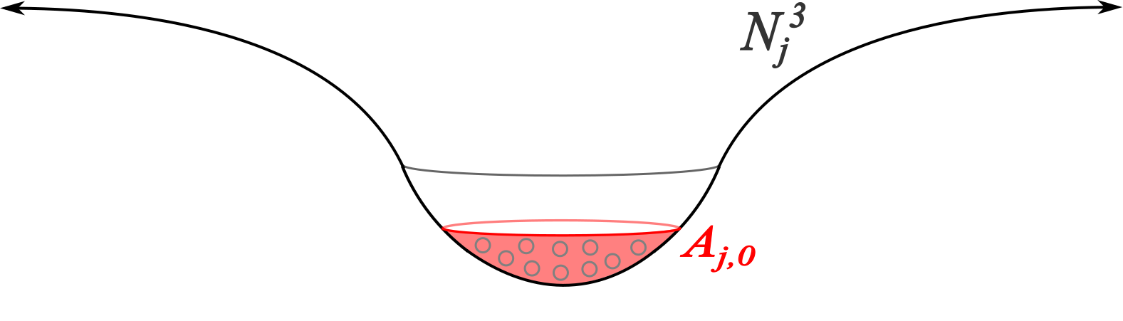
Figure 6. An element of the sequence of asymptotically flat sewn manifolds constructed in Example 6.9.

Example 6.9.

There exists a sequence of asymptotically flat manifolds $N_{j}^{3}$ with nonnegative scalar curvature, empty boundary and $\lim_{j\to\infty}\mathrm{m}_{\mathrm{ADM}}(M_{j}^{3})=0$ that converges in the pointed Gromov-Hausdorff and pointed Intrinsic Flat sense to $\mathbb{E}^{3}$ with a closed unit $3$-ball pulled to a point $p_{0}$ in the following sense: given any $\alpha_{0}>0$ and $D>0$ suffificently large,

(145) $$d_{GH}(T_{D}(\Sigma_{\alpha_{0}})\subset N_{j}^{3},T_{D}(\Sigma_{\alpha_{0}})\subset N_{\infty})\to 0$$

and

(146) $$d_{{\mathcal{F}}}(T_{D}(\Sigma_{\alpha_{0}})\subset N_{j}^{3},T_{D}(\Sigma_{\alpha_{0}})\subset N_{\infty})\to 0$$

where $N_{\infty}$ which is $\mathbb{E}^{3}$ with a closed $3$-ball pulled to a point $p_{0}$ as in Lemma 2.2 and $\Sigma_{\alpha_{0}}$ is the surface with $\operatorname{Vol}_{2}(\Sigma_{\alpha_{0}})=\alpha_{0}$.

Proof.

Let $\alpha_{0}>0$ be given. Set

(147) $$r_{0}=\left(\frac{\alpha_{0}}{4\pi}\right)^{1/2}$$

and let $D$ be large enough that $D>r_{0}$.

Fix $j\in\mathbb{N}$. Let $\delta_{j}=1/j$ and

(148) $$r_{j,2}=0\qquad\text{and }\qquad r_{j,3}=r_{0}/2.$$

By Lemma 6.5, there exists rotationally symmetric manifolds $\bar{M}_{j}^{3}\in\operatorname{RotSym}_{3}$ with $\textrm{m}_{\textrm{ADM}}(\bar{M}_{j}^{3})<\delta_{j}$ and with constant sectional curvature $K_{j}>0$ on the stripe

(149) $$r^{-1}(0,b_{j})\subset r^{-1}[r_{j,2},r_{j,3}],$$

for some $a_{j}=0<b_{j}$ in the interval $[r_{j,2},r_{j,3}]$.

Let $M_{j}^{3}=Cl(T_{D}(\Sigma_{j,0}))\subset\bar{M}_{j}^{3}$ and $M_{\infty}^{3}=Cl(T_{D}(\Sigma_{0}))\subset\mathbb{E}^{3}$, where $\Sigma_{j,0}$ and $\Sigma_{0}$ are the surfaces with area equal to $\alpha_{0}$ and, thus, are at a distance of $r_{0}$ from the axis (in graphical coordinates). Further, let $A_{j,0}$ be closed 3-ball $r^{-1}(0,b_{j}/2)$ in $M_{j}^{3}$. Let $A_{\infty,0}$ be 3-ball centered at $0$ in $\mathbb{E}^{3}$ of radius $r_{0}/2$. Observe that by our choices in (147) and (148) the stripe of constant sectional curvature $r^{-1}(0,b_{j})$ always belongs to $M_{j}$ (including $j=\infty)$ and it is at the bottom.

The tubular neighborhoods $M_{j}^{3}$ and $M_{\infty}^{3}$ are isometrically embedded into $\mathbb{E}^{4}$ by Lemma 6.2, so there exist biLipschitz maps $\psi_{j}:M_{j}^{3}\to M_{\infty}^{3}$ with $\psi_{j}(A_{j,0})=A_{\infty,0}$ and (100). Moreover, $M_{j}^{3}$ and $M_{\infty}^{3}$ are compact, so we can apply Theorem 5.1 to obtain a sequence of sewn manifolds $N_{j}^{3}$ satisfying

(150) $$d_{GH}(N_{j}^{3},N_{\infty})\to 0$$

and

(151) $$d_{{\mathcal{F}}}(N_{j}^{3},N_{\infty})\to 0$$

where $N_{\infty}$ is $M_{\infty}$ with the ball $A_{\infty,0}$ pulled to a point $p_{0}$ as in Proposition 2.1. ∎

References

- [Bam16] Richard Bamler. A Ricci flow proof of a result by Gromov on lower bounds for scalar curvature. Mathematical Research Letters, 23(2):325–337, 2016.
- [BBI01] Dmitri Burago, Yuri Burago, and Sergei Ivanov. A course in metric geometry, volume 33 of Graduate Studies in Mathematics. American Mathematical Society, Providence, RI, 2001.
- [BDS18] Jorge Basilio, Józef Dodziuk, and Christina Sormani. Sewing riemannian manifolds with positive scalar curvature. Journal of Geometric Analysis, 28:3553–3602, December 2018.
- [BI09] Dimitri Burago and Sergei Ivanov. Area spaces: First steps, with appendix by nigel higson. Geometric and Functional Analysis, 19(3):662–677, 2009.
- [BKS19] Jorge Basilio, Demetre Kazaras, and Christina Sormani. An intrinsic flat limit of riemannian manifolds with no geodesics. to appear in Geometriae Dedicata, 2019.
- [BS19] Jorge Basilio and Christina Sormani. Tori that are limits of manifolds with almost nonnegative scalar curvature. to appear, 2019.
- [GL80] Mikhael Gromov and H. Blaine Lawson, Jr. Spin and scalar curvature in the presence of a fundamental group. I. Ann. of Math. (2), 111(2):209–230, 1980.
- [Gro99] Misha Gromov. Metric structures for Riemannian and non-Riemannian spaces, volume 152 of Progress in Mathematics. Birkhäuser Boston Inc., Boston, MA, 1999. Based on the 1981 French original [ MR0682063 (85e:53051)], With appendices by M. Katz, P. Pansu and S. Semmes, Translated from the French by Sean Michael Bates.
- [Gro14] Misha Gromov. Plateau-Stein manifolds. Cent. Eur. J. Math., 12(7):923–951, 2014.
- [HLS16] Lan-Hsuan Huang, Dan Lee, and Christina Sormani. Stability of the positive mass theorem for graphical hypersurfaces of Euclidean space. to appear Journal fur die Riene und Angewandte Mathematik, 2016.
- [JL19] Jeff Jauregui and Dan A. Lee. Lower semicontinuity of adm mass under intrinsic flat convergence. arXiv:1903.00916, 2019.
- [LS12] Dan A. Lee and Christina Sormani. Near-equality of the Penrose inequality for rotationally symmetric Riemannian manifolds. Ann. Henri Poincaré, 13(7):1537–1556, 2012.
- [LS14] Dan A. Lee and Christina Sormani. Stability of the positive mass theorem for rotationally symmetric riemannian manifolds. Journal fur die Riene und Angewandte Mathematik (Crelle’s Journal), 686, 2014.
- [LS15] Philippe G. LeFloch and Christina Sormani. The nonlinear stability of rotationally symmetric spaces with low regularity. J. Funct. Anal., 268(7):2005–2065, 2015.
- [MS14] Mantoulidis and Schoen. On the bartnik mass of apparent horizons. Classical and Quantum Gravity 32(20), 2014.
- [Sor14] Christina Sormani. Intrinsic flat Arzela-Ascoli theorems. to appear in Communications in Analysis and Geometry, arXiv:1402.6066, 2014.
- [Sor17] Christina Sormani. Scalar curvature and intrinsic flat convergence Chapter 9 in Measure Theory in Non-Smooth Spaces, edited by Nicola Gigli, De Gruyter Press, pp 288-338. arXiv:1606.08949, 2017.
- [SS17] C Sormani and I Stavrov. Geometrostatic manifolds of small ADM mass. to appear, 2017.
- [SW11] Christina Sormani and Stefan Wenger. Intrinsic flat convergence of manifolds and other integral current spaces. Journal of Differential Geometry, 87, 2011.
- [SY79a] R. Schoen and S. T. Yau. On the structure of manifolds with positive scalar curvature. Manuscripta Math., 28(1-3):159–183, 1979.
- [SY79b] Richard Schoen and Shing Tung Yau. On the proof of the positive mass conjecture in general relativity. Comm. Math. Phys., 65(1):45–76, 1979.