From Robustness to Learnability: a General Approach to the Sample Complexity in Multi-item Auctions

Learnability and Robustness of Multi-Item Mechanisms without Item-Independence

Multi-Item Mechanisms without Item-Independence: Robustness implies Learnability

Multi-Item Mechanisms without Item-Independence: Learnability via Robustness

Abstract

We study the sample complexity of learning revenue-optimal multi-item auctions. We obtain the first set of positive results that go beyond the standard but unrealistic setting of item-independence. In particular, we consider settings where bidders’ valuations are drawn from correlated distributions that can be captured by Markov Random Fields or Bayesian Networks – two of the most prominent graphical models. We establish parametrized sample complexity bounds for learning an up-to-$\varepsilon$ optimal mechanism in both models, which scale polynomially in the size of the model, i.e. the number of items and bidders, and only exponential in the natural complexity measure of the model, namely either the largest in-degree (for Bayesian Networks) or the size of the largest hyper-edge (for Markov Random Fields).

We obtain our learnability results through a novel and modular framework that involves first proving a robustness theorem. We show that, given only “approximate distributions” for bidder valuations, we can learn a mechanism whose revenue is nearly optimal simultaneously for all “true distributions” that are close to the ones we were given in Prokhorov distance. Thus, to learn a good mechanism, it suffices to learn approximate distributions. When item values are independent, learning in Prokhorov distance is immediate, hence our framework directly implies the main result of Gonczarowski and Weinberg [36]. When item values are sampled from more general graphical models, we combine our robustness theorem with novel sample complexity results for learning Markov Random Fields or Bayesian Networks in Prokhorov distance, which may be of independent interest. Finally, in the single-item case, our robustness result can be strengthened to hold under an even weaker distribution distance, the Lévy distance.

1 Introduction

A central problem in Economics and Computer Science is the design of revenue-optimal auctions. The problem involves a seller who wants to sell one or more items to one or more strategic bidders. As bidders’ valuation functions are private, no meaningful revenue guarantee can be achieved without any information about these functions. To remove this impossibility, it is standard to make a Bayesian assumption, whereby a joint distribution from which bidders’ valuations are drawn is assumed common knowledge, and the goal is to design an auction that maximizes expected revenue with respect to this distribution.

In the single-item setting, a celebrated result by Myerson characterizes the optimal auction when bidder values are independent [49]. The quest for optimal multi-item auctions has been quite more challenging. It has been recognized that revenue-optimal multi-item auctions can be really complex and may exhibit counter-intuitive properties [39, 40, 9, 22, 23]. As such, it is doubtful that there is a clean characterization similar to Myerson’s for the optimal multi-item auction. On the other hand, there has been significant recent progress in efficient computation of revenue-optimal auctions [18, 19, 2, 10, 3, 12, 13, 16, 14, 4, 8, 24]. This progress has enabled the identification of simple auctions (mostly variants of sequential posted pricing mechanisms) that achieve constant factor approximations to the optimum revenue [6, 56, 15, 20, 17], under item-independence assumptions.

Making Bayesian assumptions in the study of revenue-optimal auctions is both crucial and fruitful. However, to apply the theory to practice, we would need to know the underlying distributions. Where does such knowledge come from? A common answer is that we estimate the distributions through market research or observation of bidder behavior in previously run auctions. Unavoidably, errors will creep in to the estimation, and a priori it seems possible that the performance of our mechanisms may be fragile to such errors. This has motivated a quest for optimal or approximately optimal mechanisms under imperfect knowledge of the underlying distributions.

This problem has received lots of attention from Theory of Computation recently. The focus has been on whether optimal or approximately optimal mechanisms are learnable given sample access to the true distributions. In single-item settings, where Myerson’s characterization result applies, it is possible to learn up-to-$\varepsilon$ optimal auctions [32, 21, 46, 41, 48, 28, 52, 35]. A recent paper by Guo et al. [37] provides upper and lower bounds on the sample complexity, which are tight up to logarithmic factors, thereby rendering a nearly complete picture for the single-item case.

In multi-item settings, largely due to the lack of simple characterizations of optimal mechanisms, results have been sparser. Recent work [48, 34, 11, 55] has shown how to learn simple mechanisms which attain a constant factor of the optimum revenue using polynomially many samples in the number of bidders and items. Last year, a surprising result by Gonczarowski and Weinberg [36] shows that the sample complexity of learning an up-to-$\varepsilon$ optimal mechanism is also polynomial. However, all these results rely on the item-independence assumption mentioned earlier, which limits their applicability. A main goal of our work is the following:

1. Push the boundary of learning (approximately) optimal multi-item auctions to the important setting of item dependence.

Unfortunately, it is impossible to learn approximately optimal auctions from polynomially many samples under general item dependence. Indeed, an exponential sample complexity lower bound has been established by Dughmi et al. [31] for even a single unit-demand buyer. Arguably, however, in auction settings, as well as virtually any high-dimensional setting, the distributions that arise are not arbitrary. Arbitrary high-dimensional distributions cannot be represented efficiently, and are known to require exponentially many samples to learn or even perform the most basic statistical tests on them; see e.g. [25] for a discussion. Accordingly a large focus of Statistics and Machine Learning has been on identifying structural properties of high-dimensional distributions, which enable succinct representation, efficient learning, and efficient statistical inference. In line with this literature, we propose learning multi-item auctions under the assumption that item values are jointly sampled from a high-dimensional distribution with structure.

There are several widely-studied probabilistic frameworks which allow modeling structure in a high-dimensional distribution. In this work we consider two of the most prominent ones: Markov Random Fields (MRFs) and Bayesian Networks, a.k.a. Bayesnets, which are the two most common types of graphical models. Both MRFs and Bayesnets have been studied in Machine Learning and Statistics for decades. Both frameworks can be used to express arbitrary high-dimensional distributions. Their advantage, however, is that they are associated with natural complexity parameters which allow tuning the dependence structure in the distributions they model, from product measures all the way up to arbitrary distributions. In Figure 1, we show a very simple example illustrating how naturally these models express dependence structure in a distribution. The figure shows a Bayesnet, which samples the values of a buyer for four items. The structure of the Bayesnet implies (see Definition 8) that these values are sampled conditionally independently, conditioning on the value of the variable at the root of the Bayesnet which is the state of the buyer’s residence. The node is shaded because we assume that the corresponding variable is not observable. The pertinent question is how we might exploit the structure of the distribution, as captured by the natural complexity parameter of an MRF or a Bayesnet, to efficiently learn a good mechanism. At a high level, there are two components to the problem of learning approximately optimal auctions. One is inference from samples, i.e. extracting information about the distribution using samples. The other is mechanism design, i.e. constructing a good mechanism using the information extracted. A main goal of our work is:

1. Provide a modular approach for learning multi-item auctions which decouples the Inference and Mechanism Design components, so that one may leverage all techniques from Machine Learning and Statistics to tackle the first and, independently, leverage all techniques from Mechanism Design to address the second.

Unfortunately, the Statistical and Mechanism design components are complexly intertwined in prior work on learning multi-item auctions. Specifically, [47, 11, 55, 36] are PAC-learning approaches, which require a fine balance between (i) selecting a class of mechanisms that is rich enough to contain an approximately optimal one for a class of distributions; and (ii) having small enough statistical complexity so that the performance of all mechanisms in the class on a small sample is representative of their performance with respect to the whole distribution, and so that a small sample suffices to select a good mechanism in the class. See the related work section for a detailed discussion of these works and their natural limitations. Our goal in this work is to avoid a joint consideration of (i) and (ii). Rather we want to obtain a learning framework that separates Mechanism Design from Statistical Inference, based on the following:

1. find an algorithm ${\mathcal{M}}$, which given a distribution $F$ in some family of distributions $\mathcal{F}$, computes an (approximately) optimal mechanism ${\mathcal{M}}(F)$ when bidders’ valuations are drawn from $F$;

2. find an algorithm ${\cal L}$, which given sample access to a distribution $F$ from the family of distributions ${\cal F}$ learns a distribution ${\cal L}(F)$ that is close to $F$ in some distribution distance $d$.

Achieving (i)’ and (ii)’ is of course not enough, unless we also guarantee the following:

1. given an (approximately) optimal mechanism $M$ for some $F$ there is a way to transform $M$ to some $M^{\prime}$ that is approximately optimal for any distribution $F^{\prime}$ that is close to $F$ under distribution distance $d$.

Given (i)’–(iii)’, the learnability of (approximately) optimal mechanisms for a family of distributions ${\cal F}$ can be established as follows: (a) Given sample access to some distribution $F\in{\cal F}$ we use ${\cal L}$ to learn some distribution $F^{\prime}$ that is close to $F$ under $d$;  (b) we then use $\cal M$ to compute an (approximately) optimal mechanism $M^{\prime}$ for $F^{\prime}$; and (c) finally, we use (iii)’ to argue that $M^{\prime}$ can be converted to a mechanism $M$ that is (approximately) optimal for $F$ because $M$ is (approximately) optimal for any distribution that is close to $F^{\prime}$.

Clearly, (iii)’ is important for decoupling (i)’—i.e. computing (approximately) optimal mechanisms for a family of distributions ${\cal F}$, and (ii)’—i.e. learning distributions in ${\cal F}$. At the same time, it is important in its own right:

1. Develop robust mechanism design tools, allowing to transform a mechanism $M$ designed for some distribution $F$ into a mechanism $M_{\rm robust}$ which attains similar performance simultaneously for all distributions that are close to $F$ in some distribution distance of interest.

The reason Goal III is interesting in its own right is that oftentimes we actually have no sample access to the underlying distribution over valuations. It is possible that we estimate that distribution through market research or econometric analysis in related settings, so we only know some approximate distribution. In other settings, we may have sample access to the true distribution but there might be errors in measuring or recording those samples. In both cases, we would know some approximate distribution $F$ that is close to the true distribution under some distribution distance, and we would want to use $F$ to identify a good mechanism for the unknown distribution that is close to $F$. Clearly, outputting a mechanism $M$ that attains good performance under $F$ might be a terrible idea as this mechanism might very well overfit the details of $F$. So we need to “robustify” $M$. A similar goal was pursued in the work of Bergemann and Schlag [7], for single-item and single-bidder settings, and in the work of Cai and Daskalakis [11], for robustifying a specific class of mechanisms under item-independence. Our goal here is to provide a very general robustification result.

1.1 Our Results

We discuss our contributions in the setting of additive bidders, whose values for the items are not necessarily independent. Our results hold for quite more general valuations, including constrained additive and any family of Lipschitz valuations (Definition 2), but we do not discuss these here to avoid overloading our notation. We will denote by $n$ the number of bidders, and by $m$ the number of items. We will also assume that the bidders’ values for the items lie in some bounded interval $[0,H]$.

Our Robustness Results (cf. Goal III above).

The setting we consider is the following. We are given a collection of model distributions ${\mathcal{D}}=\{{\mathcal{D}}_{i}\}_{i\in[n]}$, one for each bidder $i=1,\ldots,n$. We do not know the true distributions ${\mathcal{\widehat{D}}}=\{{\mathcal{\widehat{D}}}_{i}\}_{i}$ sampling the valuations of the bidders, and the only information we have about each ${\mathcal{\widehat{D}}}_{i}$ is that $d({\mathcal{D}}_{i},{\mathcal{\widehat{D}}}_{i})<\varepsilon$, under some distribution distance $d(\cdot,\cdot)$—we will discuss distances shortly.

Our goal is to design a mechanism that performs well under any possible collection of true distributions $\{{\mathcal{\widehat{D}}}_{i}\}_{i}$ that are close to their corresponding distributions $\{{\mathcal{D}}_{i}\}_{i}$ under $d$. We show that there are robustification algorithms, which transform a mechanism $M$ into a robust mechanism ${\widehat{M}}$ that attains similar revenue to that of $M$ under ${\mathcal{D}}$, except that ${\widehat{M}}$’s revenue guarantee holds simultaneously for any collection ${\mathcal{\widehat{D}}}$ that is close to ${\mathcal{D}}$. Applying our robustification algorithm to the optimum mechanism for ${\mathcal{D}}$ allows us to obtain the results reported in the first three columns of Table 1. DSIC and BIC refer to the standard properties of Dominant Strategy and Bayesian Incentive Compatibility of mechanisms, IR refers to the standard notion of Individual Rationality, and $\eta$-BIC is the standard notion of approximate Bayesien Incentive Compatibility. For completeness these notions are reviewed in Appendix B.

Some remarks are in order. First, in multi-item settings, it is unavoidable that our robustified mechanism is only approximately BIC, as we do not know the true distributions. In single-item settings, the optimal mechanism is DSIC, and we can indeed robustify it into a mechanism ${\widehat{M}}$ that is DSIC. In the multi-item case, however, it is known that DSIC mechanisms sometimes can extract at most a constant fraction of the optimal revenue [57], so it is necessary to consider BIC mechanisms and the BIC property is fragile to errors in the distributions.

Second, we consider several natural distribution distances. In multi-item settings, we consider both the Prokhorov and the Total Variation distance. In single-item settings, we consider both the Lévy and the Kolmogorov distance. Please see Section 2 for formal definitions of these distances and a discussion of their relationships, and their relationship to other standard distribution distances. We note that the Lévy distance for single-dimensional distributions, and the Prokhorov distance for multi-dimensional distributions are quite permissive notions of distribution distance. This makes our robustness results for these distances stronger, automatically implying robustness results under several other common distribution distances.

Finally, en route to proving our robustness results, we show a result of independent interest, namely that the optimal revenue is continuous with respect to the distribution distances that we consider. Our continuity results are summarized in the last column of Table 1. Note that the continuity results are substantially easier to establish than the robustness results, please see Section 1.2 for details.

Setting Distance $d$ Robustness Continuity Single Item Kolmogrov $\textsc{Rev}\left({\widehat{M}},{\mathcal{\widehat{D}}}\right)\geq\text{OPT}\left({\mathcal{\widehat{D}}}\right)-O\left(nH\varepsilon\right)$ ${\widehat{M}}$ is IR and DSIC (Theorem 2) $\left\lvert\text{OPT}\left({\mathcal{\widehat{D}}}\right)-\text{OPT}\left({\mathcal{D}}\right)\right\rvert\leq O(nH\varepsilon)$ (Theorem 2) Lévy $\textsc{Rev}\left({\widehat{M}},{\mathcal{\widehat{D}}}\right)\geq\text{OPT}\left({\mathcal{\widehat{D}}}\right)-O\left(nH\varepsilon\right)$ ${\widehat{M}}$ is IR and DSIC (Theorem 1) $\left|\text{OPT}\left({\mathcal{\widehat{D}}}\right)-\text{OPT}\left({\mathcal{D}}\right)\right|\leq O(nH\varepsilon)$ (Corollary 1) Multiple Items TV $\textsc{Rev}\left({\widehat{M}},{\mathcal{\widehat{D}}}\right)\geq\text{OPT}_{\eta}\left({\mathcal{\widehat{D}}}\right)-O\left(n^{2}mH\varepsilon+nmH\sqrt{n\varepsilon}\right)$ ${\widehat{M}}$ is IR and $\eta$- BIC w.r.t. ${\mathcal{\widehat{D}}}$, where $\eta=O\left(n^{2}mH\varepsilon\right)$ (Theorem 12) $\left\lvert\text{OPT}\left({\mathcal{\widehat{D}}}\right)-\text{OPT}\left({\mathcal{D}}\right)\right\rvert\leq O\left(n^{2}mH\varepsilon+nmH\sqrt{n\varepsilon}\right)$ (Theorem 11) Prokhorov $\textsc{Rev}\left({\widehat{M}},{\mathcal{\widehat{D}}}\right)\geq\text{OPT}_{\eta}\left({\mathcal{\widehat{D}}}\right)-O\left({n\eta}+n\sqrt{{mH\eta}}\right)$ ${\widehat{M}}$ is IR and $\eta$- BIC w.r.t. ${\mathcal{\widehat{D}}}$, where $\eta=O\left(nmH\varepsilon+m\sqrt{nH\varepsilon}\right)$ (Theorem 12) $\left\lvert\text{OPT}({\mathcal{D}})-\text{OPT}({\mathcal{\widehat{D}}})\right\rvert\leq O\left(n\xi+n\sqrt{mH\xi}\right)$ where $\xi=O\left(nmH\varepsilon+m\sqrt{nH\varepsilon}\right)$ (Theorem 11)

Table 1: Summary of Our Robustness and Revenue Continuity Results. Recall that the true bidder distributions ${\mathcal{\widehat{D}}}$ are unknown, and that ${\widehat{M}}$ is the robustified mechanism returned by our algorithm given an optimal mechanism $M$ for a collection of bidder distributions ${\mathcal{D}}$ that are $\varepsilon$-close to ${\mathcal{\widehat{D}}}$ under distribution distance $d$. $\textsc{Rev}({\widehat{M}},{\mathcal{\widehat{D}}})$ denotes the revenue of ${\widehat{M}}$ when the bidder distributions are ${\mathcal{\widehat{D}}}$. For a collection of bidder distributions $\cal F$, $\text{OPT}({\cal F})$ is the optimal revenue attainable by any BIC and IR mechanism under distributions $\cal F$, and $\text{OPT}_{\eta}({\mathcal{F}})$ denotes the optimum revenue attainable by any $\eta$-BIC and IR mechanism under ${\mathcal{F}}$. Not included in the table are approximation preserving robustification results under TV and Prokhorov closeness. We show that we can transform any $c$-approximation $M$ w.r.t. ${\mathcal{D}}$ to a robust mechanism ${\widehat{M}}$, so that ${\widehat{M}}$ is almost a $c$-approximation w.r.t. ${\mathcal{\widehat{D}}}$. The results included in the table are corollaries of this more general result when $c=1$. See our theorem statements for the complete details. Moreover, if there is only a single bidder, we can strengthen our robustness results in multi-item settings so that ${\widehat{M}}$ is IC instead of $\eta$-IC (see Theorem 13). Our continuity results hold for any ${\mathcal{D}}$ and ${\mathcal{\widehat{D}}}$ as long as $d({\mathcal{D}}_{i},{\mathcal{\widehat{D}}}_{i})\leq\varepsilon$ for each bidder $i$.

Learning Multi-Item Auctions Under Item Dependence (cf. Goal I above).

In view of our robustness results, presented above, the challenge of learning near-optimal auctions given sample access to the bidders’ valuation distributions, becomes a matter of estimating these distributions in the required distribution distance, depending on which robustification result we want to apply.

When the item values are independent, learning bidders’ type distributions in our desired distribution distances is immediate. So we easily recover the guarantees of the main theorem of [36]. These guarantees are summarized in the second row of Table 2, and are expanded upon in Theorem 6.

But a main goal of our work (namely Goal I from earlier) is to push the learnability of auctions well beyond item-independence. As stated earlier, it is impossible to attain learnability from polynomially many samples for arbitrary joint distributions over item values so we consider the well-studied frameworks of MRFs and Bayesnets. These frameworks are flexible and can model any distribution, but they have a tunable complexity parameter whose value controls the dependence structure. This parameter is the maximum clique size of an MRF and maximum in-degree of a Bayesnet. We will denote this complexity parameter $d$ in both cases. Recall that we also used $d(\cdot,\cdot)$ to denote distribution distances. To disambiguate, whenever we study MRFs or Bayesnets, we make sure to use $d(\cdot,\cdot)$, with parentheses, to denote distribution distances. Note that a small value of the complexity parameter $d$ does not mean that the corresponding MRF or Bayesnet does not have correlations among every pair of item values. Many natural MRF structures, with $d=2$, and Bayesnet structures, with $d=1$, permit distributions where all the variables are correlated, and indeed any pair of variables remain correlated even after conditioning on the values of all the other variables. In Figure 1, we show a simple such example where the values of a bidder on four items are sampled from a Naive Bayes Model, which is a very simple type of Bayesnet with $d=1$. While even small values of $d$ allow all pairs of variables to be correlated even conditioning on everything else, the complexity parameter $d$ forbids arbitrary dependence structures. Indeed, this is the reason why MRFs and Bayesnets are so prevalent. They allow rich dependent structures but not arbitrary ones, unless their complexity parameter $d$ is tuned up to its maximum possible value, i.e. equal to the total number of variables, in which case they can express any dependence structure. In particular, a model of complexity $d$ can express arbitrary dependence on subsets of $d$ (for MRFs) or $d+1$ (for Bayesnets) variables, and it allows some dependence structures on larger subsets of variables depending on the graphical structure of the model.

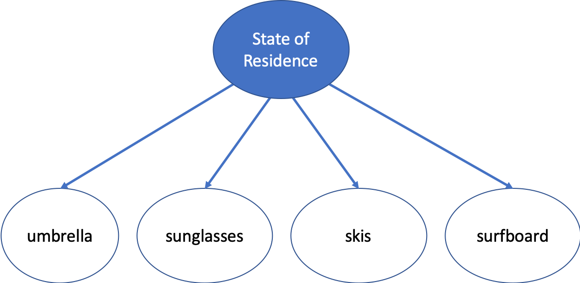
Figure 1: The values of a buyer for an umbrella, a pair of sunglasses, a pair of skis, and a surfboard are sampled from a Naive Bayes model. These values are sampled conditionally independently conditioning on the value of the variable at the root of the network, which is the state of the buyer’s residence. This variable is latent, i.e. non-observable, and this is why the corresponding node of the network is shaded blue. The distribution over $(v_{\rm umbrella},v_{\rm sunglasses},v_{\rm skis},v_{\rm surfboard})$ has the property that any pair of values remain correlated even conditioning on all the other values, unless the conditional distributions in the Bayesnet have special structure.

Now, in order to learn near-optimal mechanisms when item values for each bidder are sampled from an MRF or a Bayesnet of certain complexity $d$, our robustness results reassure us that it suffices to learn MRFs and Bayesnets under Total Variation or Prokhorov distance, depending on which multi-item robustenss theorem we seek to apply. So we need an upper bound on the sample complexity necessary to learn MRFs and Bayesnets. One of the contributions of our paper is to provide very general sample complexity bounds for learning these distributions, as summarized in Theorems 9 and 10 for MRFs and Bayesnets respectively. In both theorems, $V$ is the set of variables, $d$ is the complexity measure of the underlying distribution, and $\varepsilon$ is the distance within which we are seeking to learn the distribution. Each theorem has a version when the variables take values in a finite alphabet $\Sigma$, and a version when the variables take values in some interval $\Sigma=[0,H]$. In the first case, we provide bounds for learning in the stronger notion of Total Variation distance. In the second case, since we are learning from finitely many samples, we need to settle for the weaker notion of Prokhorov distance. For the same reason, we need to make some Lipschitzness assumption on the density, so our sample bounds depend on the Lipschitzness $\cal C$ of the MRF’s potential functions and the Bayesnet’s conditional distributions.

The sample bounds we obtain for learning MRFs and Bayesnets are directly reflected in the sample bounds we obtain for learning multi-item auctions when the item-values are sampled from an MRF or a Bayesnet respectively, as summarized in the last two rows of Table 2. Indeed, the sample complexity for learning auctions is entirely due to the sample complexity needed to learn the underlying item-distribution. In all cases we consider, the complexity is polynomial in number of variables $n=|V|$ and only depends exponentially in $d$, the complexity of the distribution, and this is unavoidable. 

Setting  Revenue Guarantee and Sample Complexity Prior Result Technique Item Independence up-to-$\varepsilon$ optimal, $\eta$-BIC (Theorem 6) ${\rm poly}\left(n,m,H,1/\varepsilon,1/\eta,\log(1/\delta)\right)$ recovers main result of [36] Prokhorov Robustness + Learnability of Product Dist. (Folklore) MRF up-to-$\varepsilon$ optimal, $\eta$-BIC (Theorem 7) ${\rm poly}\left(n,m^{d},|\Sigma|^{d},H,1/\eta,1/\varepsilon,\log(1/\delta)\right)$ (Finite $\Sigma$) ${\rm poly}\left(n,m^{d^{2}},({{\mathcal{C}}H\over\varepsilon})^{d},1/\eta,\log(1/\delta)\right)$ ($\Sigma=[0,H]$) unknown Prokhorov Robustness + Learnability of MRFs (Theorem 9) Bayesnet up-to-$\varepsilon$ optimal, $\eta$-BIC (Theorem 8) ${\rm poly}\left(n,d,m,|\Sigma|^{d+1},H,1/\eta,1/\varepsilon,\log(1/\delta)\right)$ (Finite $\Sigma$) ${\rm poly}\left(n,d^{d+1},m^{d+1},({{\mathcal{C}}H\over\varepsilon})^{d+1},1/\eta,\log(1/\delta)\right)$ ($\Sigma=[0,H]$) unknown Prokhorov Robustness + Learnability of Bayesnets (Theorem 10)

Table 2: Summary of Our Sample-based Results. We denote by $\Sigma$ the support of each item-marginal, taken to equal the interval $[0,H]$ in the continuous case, we use $\delta$ for the failure probability, and use $d$ to denote the standard complexity measure of the graphical model used to model item dependence, namely the size of the maximum hyperedge in MRFs and the largest in-degree in Bayesnets. For both MRFs and Bayesnets we allow latent variables and we also do not need to know the underlying graphical structure. Moreover, for continuous distributions, our results require Lipschitzness of potential functions in MRFs and conditional distributions in Bayesnets, which we denote with ${\mathcal{C}}$. Finally, if there is only a single bidder, the mechanism we learnt is strengthened to be IC instead of $\eta$-IC. See our theorem statements for our complete results.

Our sample bounds improve if the underlying graph of the MRF or Bayesnet are known and, importantly, without any essential modifications our sample bounds hold even when there are latent, i.e. unobserved, variables in the distribution. This makes both our auction and our distribution learning results much more richly applicable. As a simple example of the modeling power of latent variables, situations can be captured where an unobserved random variable determines the type of a bidder, and conditioning on this type the observable values of the bidder for different items are sampled.

Finally, it is worth noting that our sample bounds for learning MRFs (i.e. Theorem 9) provide broad generalizations of the bounds for learning Ising models and Gaussian MRFs presented in recent work of Devroye et al [30]. Their bounds are obtained by bounding the VC complexity of the Yatracos class induced by the distributions of interest, while our bounds are obtained by constructing $\varepsilon$-nets of the distributions of interest, and running a tournament-style hypothesis selection algorithm [29, 26, 1] to select one distribution from the net. Since the distribution families we consider are non-parametric, our main technical contribution is to bound the size of an $\varepsilon$-net sufficient to cover the distributions of interest. Interestingly, we use properties of linear programs to argue through a sequence of transformations that the net size can be upper bounded in terms of the bit complexity of solutions to a linear program that we construct.

1.2 Roadmap and Technical Ideas

In this section, we provide a roadmap to the paper and survey some of our technical ideas.

Single-item Robustness (Appendix 3)

We consider first the setting where the model distribution ${\mathcal{D}}$ is $\varepsilon$-close to the true, but unknown distribution ${\mathcal{\widehat{D}}}$ in Kolmogorov distance. In this case, we argue directly that Myerson’s optimal mechanism [49] for ${\mathcal{D}}$ is approximately optimal for any distribution that is in the $\varepsilon$-Kolmogorov-ball around ${\mathcal{D}}$, which includes ${\mathcal{\widehat{D}}}$ (Theorem 2). The idea is that the revenue of the optimal mechanism can be written as an integral over probabilities of events of the form: does $v_{i}$ lie in a certain interval $[a,b]$? Since ${\mathcal{D}}$ and ${\mathcal{\widehat{D}}}$ are $\varepsilon$-close in Kolmogorov distance, the probabilities of all such events are within $\varepsilon$ of each other, which implies that the revenues under ${\mathcal{D}}$ and ${\mathcal{\widehat{D}}}$ are also close. Finally, note that Myerson’s optimal mechanism is DSIC and IR, so it is truthful and IR w.r.t. any distribution.

Unfortunately, the same idea fails for Lévy distance, as the difference in the probabilities of the event that a certain $v_{i}$ lies in some interval $[a,b]$ under ${\mathcal{D}}$ and ${\mathcal{\widehat{D}}}$ can be as large as $1$ even when ${\mathcal{D}}$ and ${\mathcal{\widehat{D}}}$ are $\varepsilon$-close in Lévy distance. (Indeed, consider two single point distributions: a point mass at $A$ and a point mass at $A-\varepsilon$; their probabilities of falling in the interval $[A-\varepsilon/2,A+\varepsilon/2]$ are respectively $1$ and $0$.) We thus prove our robustness result for Lévy distance via a different route. Given any model distribution ${\mathcal{D}}$, we first construct the “worst” distribution ${\underline{\mathcal{D}}}$ and the “best” distribution ${\overline{\mathcal{D}}}$ in the $\varepsilon$-Lévy ball around ${\mathcal{D}}$: this means that, for any ${\mathcal{\widehat{D}}}$ that lies in the $\varepsilon$-Lévy ball around ${\mathcal{D}}$, ${\mathcal{\widehat{D}}}$ first-order stochastically dominates ${\underline{\mathcal{D}}}$ and is dominated by ${\overline{\mathcal{D}}}$ (see Definition 3). We choose our robust mechanism ${\widehat{M}}$ to be Myerson’s optimal mechanism for ${\underline{\mathcal{D}}}$. It is not hard to argue that ${\widehat{M}}$’s revenue under ${\mathcal{\widehat{D}}}$ is at least $\text{OPT}({\underline{\mathcal{D}}})$, the optimal revenue under the “worst” distribution (Lemma 4), due to the revenue monotonicity lemma (Lemma 3) shown in [28]. The statement provides a lower bound of ${\widehat{M}}$’s revenue under the unknown true distribution ${\mathcal{\widehat{D}}}$. To complete the argument, we need to argue that $\text{OPT}({\mathcal{\widehat{D}}})$ cannot be too much larger than $\text{OPT}({\underline{\mathcal{D}}})$. Indeed, we relax $\text{OPT}({\mathcal{\widehat{D}}})$ to $\text{OPT}({\overline{\mathcal{D}}})$, and show that even the optimal revenue under the “best” distribution $\text{OPT}({\overline{\mathcal{D}}})\approx\text{OPT}({\underline{\mathcal{D}}})$. To do so, we construct two auxiliary distributions $P$ and $Q$, such that (i) $\text{OPT}(P)\approx\text{OPT}(Q)$; and (ii) $P$ and ${\underline{\mathcal{D}}}$ are $\varepsilon$-close in Kolmogorov distance, and $Q$ and ${\overline{\mathcal{D}}}$ are $\varepsilon$-close also in Kolmogorov distance. Our robustness theorem under Kolmogorov distance (Theorem 2) implies then that $\text{OPT}(P)\approx\text{OPT}({\underline{\mathcal{D}}})$ and $\text{OPT}(Q)\approx\text{OPT}({\overline{\mathcal{D}}})$. Hence, $\text{OPT}({\overline{\mathcal{D}}})\approx\text{OPT}({\underline{\mathcal{D}}})$, which completes our proof.

Multi-item Robustness (Section 4)

We first discuss our result for total variation distance. Unfortunately, our approach for Lévy distance—of simply choosing the optimal mechanism for the “worst,” in the first-order stochastic dominance sense, distribution in the $\varepsilon$-TV-ball around ${\mathcal{D}}$ to be our robust mechanism—no longer applies. Indeed, it is known that the optimal revenue in multi-item auctions may be non-monotone with respect to first-order stochastic dominance [40], i.e. a distribution may be stochastically dominated by another but result in higher revenue. However, if ${\mathcal{D}}$ and ${\mathcal{\widehat{D}}}$ are $\varepsilon$-close in total variation distance, this means that there is a coupling between ${\mathcal{D}}$ and ${\mathcal{\widehat{D}}}$ under which the valuation profiles are almost always sampled the same. If we take the optimal mechanism $M$ for ${\mathcal{D}}$, and apply to bidders from ${\mathcal{\widehat{D}}}$, it will produce almost the same revenue under ${\mathcal{\widehat{D}}}$, and vice versa. Indeed, the only event under which $M$ may generate different revenue under the two distributions is when the coupling samples different profiles, but this happens with small probability. Similarly, the BIC and IR properties of $M$ under ${\mathcal{D}}$ become slightly approximate under ${\mathcal{\widehat{D}}}$. We claim that we can massage $M$, in a way oblivious to ${\mathcal{\widehat{D}}}$, to produce a $\left({\rm poly}(n,m,H)\cdot\varepsilon\right)$-truthful and exactly IR mechanism ${\widehat{M}}$ for ${\mathcal{\widehat{D}}}$, which achieves an up-to-$\left({\rm poly}(n,m,H)\cdot\varepsilon\right)$ revenue (Theorem 3).

The main challenge is when ${\mathcal{D}}$ and ${\mathcal{\widehat{D}}}$ are only $\varepsilon$-close in Prokhorov distance. Note that two distributions within Prokhorov distance $\varepsilon$ may have total variation distance $1$. Just imagine two point masses: one at $A$ and another at $A-\varepsilon$. So Prokhorov robustness is not directly implied by TV robustness.

Why Standard Discretization Arguments are Insufficient?

Unlike standard algorithmic problems, discretization is subtle in mechanism design. Due to the presence of incentives, a small change in the bidders’ value distributions may change the distribution of outcomes of the mechanism dramatically. To perform discretization in mechanism design, a standard procedure goes as follows [5, 36, 45]: let ${\mathcal{\widehat{D}}}$ be the true distribution, and ${\mathcal{D}}$ be the distribution after discretization; design the optimal mechanism $M$ for ${\mathcal{D}}$; to run $M$ on a bid vector $b$ from ${\mathcal{\widehat{D}}}$, discretize it to $\gamma(b)=({\gamma}_{1}(b_{1}),\ldots,{\gamma}_{n}(b_{n}))$ and apply mechanism $M$ on $\gamma(b)$. This procedure can be generalized to any pair of distributions ${\mathcal{D}}$ and ${\mathcal{\widehat{D}}}$ as long as, we are given a coupling $\gamma(\cdot)$ between ${\mathcal{D}}$ and ${\mathcal{\widehat{D}}}$ that maps any bid vector $b$ in the support of distribution ${\mathcal{\widehat{D}}}$ to a bit vector $\gamma(b)$ in the support of ${\mathcal{D}}$. If for every bidder $i$, $b_{i}$ and ${\gamma}_{i}(b_{i})$ are close with all but small probability, we can apply similar arguments as in the total variation robustness result to massage the mechanism above to be nearly-truthful and exactly IR for ${\mathcal{\widehat{D}}}$, and argue it is approximately revenue optimal. Clearly, in the context of discretization, $b_{i}$ and $\gamma_{i}(b_{i})$ are guaranteed to be close if the discretization is sufficiently fine.

At first glance, this procedure may seem applicable to our problem. A characterization of Prokhorov distance due to Strassen (Theorem 4) shows that: two distributions $P$ and $Q$ are $\varepsilon$-close in Prokhorov distance if and only if there exists a (potentially randomized) coupling $\gamma$ such that if random variable $s$ is distributed according to $P$, then $\gamma(s)$ is distributed according to $Q$ and $\Pr\left[\left\lVert s-\gamma(s)\right\rVert_{1}>\varepsilon\right]\leq\varepsilon$. If $M$ is the optimal mechanism for the model distribution ${\mathcal{D}}$, and ${\mathcal{\widehat{D}}}$ is the true distribution that is $\varepsilon$-close to ${\mathcal{D}}$, why can’t we combine the procedure above with the coupling $\gamma$ to establish our Prokhorov robustness result?

Unfortunately, this approach is insufficient due to the following two issues: (i) The procedure relies on knowing the coupling ${\gamma}$. As we do not even know ${\mathcal{\widehat{D}}}$, how can we know the coupling? (ii) Even if we can identify the coupling $\gamma$ between ${\mathcal{D}}$ and a specific ${\mathcal{\widehat{D}}}$, the procedure above constructs a mechanism that depends on the coupling $\gamma$. However, ${\gamma}$ may change for every different ${\mathcal{\widehat{D}}}$ in the $\varepsilon$-Prokhorov-ball around ${\mathcal{D}}$, so the procedure generates a different mechanism for every possible true distribution. 

To satisfy our requirement for a robust mechanism in Goal III, we need to construct a single mechanism that is nearly truthful, IR, and near-optimal simultaneously for every distribution in the $\varepsilon$-Prokhorov-ball around ${\mathcal{D}}$. Our proof relies on a novel way to “simultaneously couple” ${\mathcal{D}}$ with every distribution ${\mathcal{\widehat{D}}}$ in the $\varepsilon$-Prokhorov-ball around ${\mathcal{D}}$. If we round both ${\mathcal{D}}$ and any ${\mathcal{\widehat{D}}}$ to a random grid $G$ with width $\sqrt{\varepsilon}$, we can argue that the expected total variation distance (over the randomness of the grid) between the two rounded distributions ${\mathcal{D}}_{G}$ and ${\mathcal{\widehat{D}}}_{G}$ is $O(\sqrt{\varepsilon})$ (Lemma 7). Now consider the following mechanism: choose a random grid $G$, round the bids to the random grid, apply the optimal mechanism $M_{G}$ that is designed for ${\mathcal{D}}_{G}$. Our robustness result under the total variation distance implies that for every realization of the random grid $G$, $M_{G}$ is $O\left({\rm poly}(n,m,H)\cdot\left\lVert{\mathcal{D}}_{G}-{\mathcal{\widehat{D}}}_{G}\right\rVert_{TV}\right)$-truthful and up-to-$O\left({\rm poly}(n,m,H)\cdot\left\lVert{\mathcal{D}}_{G}-{\mathcal{\widehat{D}}}_{G}\right\rVert_{TV}\right)$ revenue optimal for any ${\mathcal{\widehat{D}}}_{G}$. Since the expected value (over the randomness of the grid) of $\left\lVert{\mathcal{D}}_{G}-{\mathcal{\widehat{D}}}_{G}\right\rVert_{TV}$ is $O(\sqrt{\varepsilon})$ for any ${\mathcal{\widehat{D}}}$ in the $\varepsilon$-Prokhorov-ball of ${\mathcal{D}}$, our randomized mechanism is simultaneously $O\left({\rm poly}(n,m,H)\cdot\sqrt{\varepsilon}\right)$-truthful and up-to-$O\left({\rm poly}(n,m,H)\cdot\sqrt{\varepsilon}\right)$ revenue optimal for all distributions in the $\varepsilon$-Prokhorov-ball around ${\mathcal{D}}$.

Sample Complexity Results

In Section 5, we apply our robustness theorem to obtain sample bounds for learning multi-item auctions under the item-independence assumption (Theorem 6). Our result provides an alternative proof of the main result of [36]. In Section 7, we combine our robustness theorem with our sample bounds for learning Markov Random Fields and Bayesian Networks discussed earlier to derive new polynomial sample complexity results for learning multi-item auctions when the distributions have structured correlation over the items. Theorem 7 summarizes our results when item values are generated by an MRF, and Theorem 8 our results when item values are generated by a Bayesenet.

2 Preliminaries

We first define a series statistical distances that we will use in the paper and discuss their relationships.

Definition 1 (Statistical Distance).

Let $P$ and $Q$ be two probability measures. We use $\left\lVert P-Q\right\rVert_{TV}$, $\left\lVert P-Q\right\rVert_{K}$, and $\left\lVert P-Q\right\rVert_{L}$ to denote the total variational distance, the Kolmogorov distance, and the Lévy distance between $P$ and $Q$, respectively. See Appendix B for more details. Prokhorov Distance is a generalization of the Lévy Distance to high dimensional distributions. Let $(U,d)$ be a metric space and $\cal{B}$ be a $\sigma$-algebra on $U$. For $A\in\cal{B}$, let $A^{\varepsilon}=\{x:\exists y\in A\ \ s.t\ \ d(x,y)<\varepsilon\}$. Then two measures $P$ and $Q$ on $\cal{B}$ have Prokhorov distance

$$\inf\left\{\varepsilon>0:P(A)\leq Q(A^{\varepsilon})+\varepsilon,\ Q(A)\leq P(A^{\varepsilon})+\varepsilon\ \forall A\in\cal{B}\right\}$$

We consider distributions supported on $\mathbb{R}^{k}$ for some $k\in\mathbb{N}$, so $U$ will be the $k$-dimensional Euclidean Space, and we choose $d$ to be the $\ell_{1}$-distance. We denote the Prokhorov distance between distributions ${\mathcal{F}}$, $\widehat{{\mathcal{F}}}$ by $\left\lVert{\mathcal{F}}-\widehat{{\mathcal{F}}}\right\rVert_{P}$.

Relationships between the Statistical Distances:

Among the four metrics, the Lévy distance and the Kolmogorov distance are only defined for single dimensional distributions, while the Prokhorov distance and the total variation distance are defined for general distributions. In the single dimensional case, the Lévy distance is a very liberal metric. In particular, for any two single dimensional distributions $P$ and $Q$,

$$\left\lVert P-Q\right\rVert_{L}\leq\left\lVert P-Q\right\rVert_{K}\leq\left\lVert P-Q\right\rVert_{TV}.$$

Note that a robustness result for a more liberal metric is more general. For example, the robustness result for single-item auctions under the Lévy metric implies the robustness under the total variation and Kolmogorov metric, because the $\varepsilon$-ball in Lévy distance contains the $\varepsilon$-ball in total variation and Kolmogorov distance. An astute reader may wonder whether one can find a more liberal metric in the single dimensional case. Interestingly, for the most common metrics studied probability theory, including the Wasserstein distance, the Hellinger distance, and the relative entropy, the Lévy distance is the most liberal up to a polynomial factor. That is, if the Lévy distance is $\varepsilon$, the distance under any of these metrics is at least ${\rm poly}(\varepsilon)$. Indeed, the polynomial is simply the identity function or the quadratic function $\varepsilon^{2}$ in most cases. Please see the survey by Gibbs and Su [33] and the references therein for more details.

The Prokhorov distance, also known as Lévy-Prokhorov Distance, is the generalization of the Lévy distance to multi-dimensional distributions. It is also the standard metric in robust statistical decision theory, see Huber [42] and Hampel et al. [38]. The Prokhorov distance is almost as liberal as the Lévy distance.  First, for any two distributions $P$ and $Q$,

$$\left\lVert P-Q\right\rVert_{P}\leq\left\lVert P-Q\right\rVert_{TV}.$$

Second, if we consider other well studied metrics such as the Wasserstein distance, the Hellinger distance, and the relative entropy, the Prokhorov distance is again the most liberal up to a polynomial factor.

Multi-item Auctions:

We focus on revenue maximization in the combinatorial auction with $n$ bidders and $m$ heterogenous items. We use $X$ to denote the set of possible allocations, and each bidder $i\in[n]$ has a valuation function/type $v_{i}(\cdot):X\mapsto\mathbb{R}_{\geq 0}$. In this paper, we assume the function $v_{i}(\cdot)$ is parametrized by $(v_{i,1},\ldots,v_{i,m})$, where $v_{i,j}$ is bidder $i$’s value for item $j$. We assume that bidder’s types are distributed independently. Throughout this paper, we assume all bidders types lie in $[0,H]^{m}$. We adopt the valuation model in Gonczarowski and Weinberg [36] and consider valuations that satisfy the following Lipschitz property.

Definition 2 (Lipschitz Valuations).

There exists an absolute constant ${\mathcal{L}}$ such that if type $\mathbb{v_{i}}=(v_{i,1},\ldots,v_{i,m})$ and $\mathbb{v^{\prime}_{i}}=(v^{\prime}_{i,1},\ldots,v^{\prime}_{i,m})$ are within $\ell_{1}$ distance $\varepsilon$, then for the corresponding valuations $v_{i}(\cdot)$ and $v^{\prime}_{i}(\cdot)$, $|v_{i}(x)-v^{\prime}_{i}(x)|\leq{\mathcal{L}}\cdot\varepsilon$ for all $x\in X$.

This for example includes common settings such as additive and unit demand with Lipschitz constant ${\mathcal{L}}=1$. More generally, ${\mathcal{L}}=1$ holds for constrained additive valuations  and even in some settings with complementarities. Please see [36] for further discussion.

A mechanism $M$ consists of an allocation rule $x(\cdot)$ and a payment rule $p(\cdot)$. For any input bids $b=(b_{1},\ldots,b_{n})$, the allocation rule outputs a distribution over allocations $x(b)\in\Delta(X)$ and payments $p(b)=\left(p_{1}(b),\ldots,p_{n}(b)\right)$. If bidder $i$’s type is $v_{i}$, her utility under input $b$ is $u_{i}\left(v_{i},M(b)\right)={\mathbb{E}}\left[v_{i}\left(x(b)\right)-p_{i}(b)\right]$.

Truthfulness and Revenue:

We use the standard notion $\varepsilon$-BIC and IR (see Appendix B for details). If $M$ is a $\varepsilon$-BIC mechanism w.r.t. some distribution ${\mathcal{D}}$, we use $\textsc{Rev}_{T}(M,{\mathcal{D}})$ to denote the revenue of mechanism $M$ under distribution ${\mathcal{D}}$ assuming bidders are bidding truthfully. Clearly, $\textsc{Rev}_{T}(M,{\mathcal{D}})=\textsc{Rev}(M,{\mathcal{D}})$ when $M$ is BIC w.r.t. ${\mathcal{D}}$. We denote the optimal revenue achievable by any $\varepsilon$-BIC (or BIC) mechanism by $\text{OPT}_{\varepsilon}({\mathcal{D}})$ (or $\text{OPT}({\mathcal{D}})$). Although it is conceivable that permitting mechanisms to be $\varepsilon$-BIC allows for much greater expected revenue than if they were restricted to be BIC, past results show that this is not the case.

Lemma 1.

[27, 53] In any $n$-bidder $m$-item auction, let ${\mathcal{D}}$ be any joint distribution over arbitrary ${\mathcal{L}}$-Lipschitz valuations, where the valuations of different bidders are independent. The maximum revenue attainable by any IR and $\varepsilon$-BIC auction for a given product distribution is at most $2n\sqrt{m{\mathcal{L}}H\varepsilon}$ greater than the maximum revenue attainable by any IR and BIC auction for that distribution.

Notations:

We allow the bidders to submit a special type $\perp$, which represents not participating the auction. If anyone submits $\perp$, the mechanism terminates immediately, and does not allocate any item to any bidder or charge any bidder. A bidder’s utility for submitting type $\perp$ is $0$. We will sometimes refer to $\perp$ as the IR type.Throughout the paper, we use ${\mathcal{\widehat{D}}}=\bigtimes_{i=1}^{n}{\mathcal{\widehat{D}}}_{i}$ to denote the true type distributions of the bidders. We use ${\mathcal{D}}=\bigtimes_{i=1}^{n}{\mathcal{D}}_{i}$ to denote the model type distributions or our learned type distributions from samples. We use ${\mathcal{D}}_{i}\mid\bigtimes_{j=1}^{m}[w_{ij},w_{ij}+\delta)$ to denote the distribution induced by ${\mathcal{D}}_{i}$ conditioned on being in the $m$-dimensional cube $\bigtimes_{j=1}^{m}[w_{ij},w_{ij}+\delta)$, and $\text{supp}({\mathcal{F}})$ to denote the support of distribution ${\mathcal{F}}$.

3 Lévy-Robustness for Single-Item Auctions

In this section, we show the robustness result under the Lévy distance in the single-item setting. If we are given a model distribution ${\mathcal{D}}_{i}$ that is $\varepsilon$-close to the true distribution ${\mathcal{\widehat{D}}}_{i}$, in Lévy distance, for every bidder $i\in[n]$, we show how to design a mechanism $M^{*}$ only based on ${\mathcal{D}}=\bigtimes_{i=1}^{n}{\mathcal{D}}_{i}$ and extracts revenue that is at most $O(nH\cdot\varepsilon)$ less than the optimal revenue under any possible true distribution ${\mathcal{\widehat{D}}}=\bigtimes_{i=1}^{n}{\mathcal{\widehat{D}}}_{i}$.

Theorem 1 (Lévy-Robustness for Single-item Auctions).

Given ${\mathcal{D}}=\bigtimes_{i=1}^{n}{\mathcal{D}}_{i}$, where ${\mathcal{D}}_{i}$ is an arbitrary distributions supported on $[0,H]$ for all $i\in[n]$. We can design a DSIC and IR mechanism $M^{*}$ based on ${\mathcal{D}}$ such that for any product distribution ${\mathcal{\widehat{D}}}=\bigtimes_{i=1}^{n}{\mathcal{\widehat{D}}}_{i}$ satisfying $\left\lVert{\mathcal{D}}_{i}-{\mathcal{\widehat{D}}}_{i}\right\rVert_{L}\leq\varepsilon$ for all $i\in[n]$, we have:

$$\textsc{Rev}(M^{*},{\mathcal{\widehat{D}}})\geq\text{OPT}({\mathcal{\widehat{D}}})-O(nH\cdot\varepsilon).$$

Let us sketch the proof of Theorem 1. We prove our statement in three steps.

• Step (i): We first identify the “best” and “worst” distributions (Definition 3), in terms of the first-order stochastic dominance (Definition 4), among all distributions in the $\varepsilon$-Lévy-ball around the model distribution ${\mathcal{D}}$. We construct the optimal mechanism $M^{*}$ w.r.t. the “worst” distribution, and show that its revenue under any possible true distribution is at least $M^{*}$’s revenue under the “worst” distribution (Lemma 4). The statement provides a lower bound of $M^{*}$’s revenue under the unknown true distribution. Its proof follows from the revenue monotonicity lemma (Lemma 3) shown in [28].

• Step (ii): We use the revenue monotonicity lemma again to show the optimal revenue under the true distribution ${\mathcal{\widehat{D}}}$ is upper bounded by the optimal revenue under the “best” distribution(Lemma 5).

• Step (iii): We complete the proof by argueing that $M^{*}$’s revenue under the “worst” distribution can be at most $O(nH\cdot\varepsilon)$ worst than the optimal revenue under the “best” distribution (Lemma 6). The statement follows from a robustness theorem for single-item auctions under the Kolmogorov distance (Theorem 2).

We show Step (i) and (ii) in Section 3.1 and Step (iii) in Section 3.2.

3.1 Best and Worst Distributions in the $\varepsilon$-Lévy-Ball

We formally define the “best” and “worst” distributions in the $\varepsilon$-Lévy-ball around the model distribution.

Definition 3.

For every $i\in[n]$, we define ${\overline{\mathcal{D}}}_{i}$ and ${\underline{\mathcal{D}}}_{i}$ based on ${\mathcal{D}}_{i}$. ${\overline{\mathcal{D}}}_{i}$ is supported on $[0,H+\varepsilon]$, and its CDF is defined as $F_{{\overline{\mathcal{D}}}_{i}}(x)=\max\left\{F_{{\mathcal{D}}_{i}}(x-\varepsilon)-\varepsilon,0\right\}$. ${\underline{\mathcal{D}}}_{i}$ is supported on $[-\varepsilon,H]$, and its CDF is defined as $F_{{\underline{\mathcal{D}}}_{i}}(x)=\min\left\{F_{{\mathcal{D}}_{i}}(x+\varepsilon)+\varepsilon,1\right\}$.

We provide a more intuitive interpretation of ${\overline{\mathcal{D}}}_{i}$ and ${\underline{\mathcal{D}}}_{i}$ here. To obtain ${\overline{\mathcal{D}}}_{i}$, we first shift all values in ${\mathcal{D}}_{i}$ to the right by $\varepsilon$, then we move the bottom $\varepsilon$ probability mass to $H+\varepsilon$. To obtain ${\underline{\mathcal{D}}}_{i}$, we first shift all values in ${\mathcal{D}}_{i}$ to the left by $\varepsilon$, then we move the top $\varepsilon$ probability mass to $-\varepsilon$. It is not hard to see that both ${\overline{\mathcal{D}}}_{i}$ and ${\underline{\mathcal{D}}}_{i}$ are still in the $\varepsilon$-ball around ${\mathcal{D}}_{i}$ in Lévy distance. More importantly, ${\overline{\mathcal{D}}}_{i}$ and ${\underline{\mathcal{D}}}_{i}$ are the “best” and “worst” distributions in the $\varepsilon$-Lévy-ball under first-order-stochastic-dominance.

Definition 4 (First-Order Stochastic Dominance).

We say distribution $B$ first-order stochastically dominates $A$ iff $F_{B}(x)\leq F_{A}(x)$ for all $x\in\mathbb{R}$. We use $A\preccurlyeq B$ to denote that distribution $B$ first-order stochastically dominates distribution $A$. If $\mathbf{A}=\times_{i=1}^{n}A_{i}$ and $\mathbf{B}=\times_{i=1}^{n}B_{i}$ are two product distributions, and $A_{i}\preccurlyeq B_{i}$ for all $i\in[n]$, we slightly abuse the notation $\preccurlyeq$ to write $\mathbf{A}\preccurlyeq\mathbf{B}$.

Lemma 2.

For any ${\mathcal{\widehat{D}}}_{i}$, such that $\left\lVert{\mathcal{\widehat{D}}}_{i}-{\mathcal{D}}_{i}\right\rVert_{L}\leq\varepsilon$, we have ${\underline{\mathcal{D}}}_{i}\preccurlyeq{\mathcal{\widehat{D}}}_{i}\preccurlyeq{\overline{\mathcal{D}}}_{i}$.

Proof.

It follows from the definition of Lévy distance and Definition 3. For any $x$,

$$F_{{\mathcal{\widehat{D}}}_{i}}(x)\in[F_{{\mathcal{D}}_{i}}(x-\varepsilon)-\varepsilon,F_{{\mathcal{D}}_{i}}(x+\varepsilon)+\varepsilon].$$

Clearly, $0\leq F_{{\mathcal{\widehat{D}}}_{i}}(x)\leq 1$, so we have $F_{{\overline{\mathcal{D}}}_{i}}(x)\leq F_{{\mathcal{\widehat{D}}}_{i}}(x)\leq F_{{\underline{\mathcal{D}}}_{i}}(x)$ for all $x$. ∎

The plan is to construct the optimal mechanism for ${\underline{\mathcal{D}}}=\bigtimes_{i=1}^{n}{\underline{\mathcal{D}}}_{i}$ and show that this mechanism achieves up-to-$O(nH\cdot\varepsilon)$ optimal revenue under any possible true distribution ${\mathcal{D}}$.

Next, we state a revenue monotonicity lemma that will be useful. We first need the following definition.

Definition 5 (Extension of a Mechanism to All Values).

Suppose a mechanism $M=(x,p)$ is defined for all value profiles in $T=\times_{i=1}^{n}T_{i}$. Define its extension $M^{\prime}=(x^{\prime},p^{\prime})$ to all values. We only specify $x^{\prime}$, as $p^{\prime}$ can be determined by the payment identity given $x^{\prime}$. $x^{\prime}$ first rounds the bid of each bidder $i$ down to the closest value in $T_{i}$, and then apply allocation rule $x$ on the rounded bids. If some bidder $i$’s bid is smaller than the lowest value in $T_{i}$, $x^{\prime}$ does not allocate the item to any bidder.

Observe that the extension provides a DSIC and IR mechanism for all values if the original mechanism is DSIC and IR.

Lemma 3 (Strong Revenue Monotonicity [28]).

Let ${\mathcal{F}}=\bigtimes_{i=1}^{n}{\mathcal{F}}_{i}$ be a product distributions. There exists an optimal DSIC and IR mechanism $M$ for ${\mathcal{F}}$ such that, for any product distribution ${\mathcal{F}}^{\prime}=\bigtimes_{i=1}^{n}{\mathcal{F}}^{\prime}_{i}\succcurlyeq{\mathcal{F}}$,

$$\textsc{Rev}(M^{\prime},{\mathcal{F}}^{\prime})\geq\textsc{Rev}(M,{\mathcal{F}})=\text{OPT}({\mathcal{F}}).$$

$M^{\prime}$ is the extension of $M$. In particular, this implies $\text{OPT}({\mathcal{F}}^{\prime})\geq\text{OPT}({\mathcal{F}})$.

Combining Lemma 2 and 3, we show that if $M^{*}$ is the extension of the optimal mechanism for ${\underline{\mathcal{D}}}$, it achieves at least $\text{OPT}({\underline{\mathcal{D}}})$ under any distribution ${\mathcal{\widehat{D}}}$ with $\left\lVert{\mathcal{\widehat{D}}}_{i}-{\mathcal{D}}_{i}\right\rVert_{L}\leq\varepsilon$.

Lemma 4.

Let $M^{*}$ be the extension of the optimal DSIC and IR mechanism for ${\underline{\mathcal{D}}}$. For any product distribution ${\mathcal{\widehat{D}}}=\bigtimes_{i=1}^{n}{\mathcal{\widehat{D}}}_{i}$ with $\left\lVert{\mathcal{\widehat{D}}}_{i}-{\mathcal{D}}_{i}\right\rVert_{L}\leq\varepsilon$ for all $i\in[n]$, we have the following:

$$\textsc{Rev}(M^{*},{\mathcal{\widehat{D}}})\geq\text{OPT}({\underline{\mathcal{D}}}).$$

Proof.

Since ${\mathcal{\widehat{D}}}\succcurlyeq{\underline{\mathcal{D}}}$ (Lemma 2), the claim follows from Lemma 3. ∎

Lemma 4 shows that with only knowledge of the model distribution ${\mathcal{D}}$, we can design a mechanism whose revenue under any possible true distribution ${\mathcal{\widehat{D}}}$ is at least $\text{OPT}({\underline{\mathcal{D}}})$. Next, we upper bound the optimal revenue under ${\mathcal{\widehat{D}}}$ with the optimal revenue under ${\overline{\mathcal{D}}}$.

Lemma 5.

For any product distribution ${\mathcal{\widehat{D}}}$ with $\left\lVert{\mathcal{\widehat{D}}}_{i}-{\mathcal{D}}_{i}\right\rVert_{L}\leq\varepsilon$ for all $i\in[n]$, we have the following:

$$\text{OPT}({\overline{\mathcal{D}}})\geq\text{OPT}({\mathcal{\widehat{D}}}).$$

Proof.

Since ${\overline{\mathcal{D}}}\succcurlyeq{\mathcal{\widehat{D}}}$ (Lemma 2), the claim follows from Lemma 3. ∎

3.2 Comparing the Revenue of the Best and Worst Distributions

In this section, we show that our lower bound of $M^{*}$’s revenue under the true distribution ${\mathcal{\widehat{D}}}$ and our upper bound of the optimal revenue under ${\mathcal{\widehat{D}}}$ are at most $O(nH\cdot\varepsilon)$ away.

Lemma 6.

$$\text{OPT}({\underline{\mathcal{D}}})\geq\text{OPT}({\overline{\mathcal{D}}})-O(nH\cdot\varepsilon).$$

It is a priori not clear why Lemma 6 should be true, as ${\overline{\mathcal{D}}}$ is the “best” distribution and ${\underline{\mathcal{D}}}$ is the “worst” distribution in the $\varepsilon$-Lévy-ball around ${\mathcal{D}}$. We prove Lemma 6 by introducing another two auxiliary distributions $\underaccent{\wtilde}{\mathcal{D}}$ and $\widetilde{\mathcal{D}}$. In particular, we construct $\widetilde{\mathcal{D}}_{i}$ by shifting all values in ${\mathcal{D}}_{i}$ to the right by $\varepsilon$, and construct $\underaccent{\wtilde}{\mathcal{D}}_{i}$ by shifting all values in ${\mathcal{D}}_{i}$ to the left by $\varepsilon$. There are two important properties of these two new distributions: (i) one can couple $\underaccent{\wtilde}{\mathcal{D}}_{i}$ with $\widetilde{\mathcal{D}}_{i}$ so that the two random variables are always exactly $2\varepsilon$ away from each other; (ii) $\underaccent{\wtilde}{\mathcal{D}}_{i}$ and ${\underline{\mathcal{D}}}_{i}$ are within Kolmogorov distance $\varepsilon$, and $\widetilde{\mathcal{D}}_{i}$ and ${\overline{\mathcal{D}}}_{i}$ are also within Kolmogorov distance $\varepsilon$. Property (i) allows us to prove that $\left\lvert\text{OPT}(\underaccent{\wtilde}{\mathcal{D}})-\text{OPT}(\widetilde{\mathcal{D}})\right\rvert\leq 2\varepsilon$ (see Claim 2). To make use of property (ii), we prove the following robustness theorem w.r.t. the Kolmogorov distance.

Theorem 2.

For any buyer $i\in[n]$, let ${\mathcal{D}}_{i}$ and ${\mathcal{\widehat{D}}}_{i}$ be two arbitrary distributions supported on $(-\infty,H]$ such that $\left\lVert{\mathcal{D}}_{i}-{\mathcal{\widehat{D}}}_{i}\right\rVert_{K}\leq\varepsilon$. We have the following:

$$\text{OPT}\left({\mathcal{\widehat{D}}}\right)\geq\text{OPT}({\mathcal{D}})-3nH\cdot\varepsilon.$$

where ${\mathcal{D}}=\bigtimes_{i=1}^{n}{\mathcal{D}}_{i}$ and ${\mathcal{\widehat{D}}}=\bigtimes_{i=1}^{n}{\mathcal{\widehat{D}}}_{i}$.

The proof of Theorem 2 is postponed to Appendix C. Equipped with Theorem 2, we can immediately show that $\left\lvert\text{OPT}(\underaccent{\wtilde}{\mathcal{D}})-\text{OPT}({\underline{\mathcal{D}}})\right\rvert\leq O(nH\cdot\varepsilon)$ and $\left\lvert\text{OPT}(\widetilde{\mathcal{D}})-\text{OPT}({\overline{\mathcal{D}}})\right\rvert\leq O(nH\cdot\varepsilon)$. Lemma 6 follows quite easily from Claim 2 and the two inequalities above. The complete proof of Lemma 6 can be found in Appendix C.

We are now ready to prove Theorem 1.

Proof of Theorem 1: We first construct ${\underline{\mathcal{D}}}$ based on ${\mathcal{D}}$ and let $M^{*}$ be the extension of the optimal mechanism for ${\underline{\mathcal{D}}}$. By Lemma 4, we know $\textsc{Rev}(M^{*},{\mathcal{\widehat{D}}})$ is at least $\text{OPT}({\underline{\mathcal{D}}})$ for any ${\mathcal{\widehat{D}}}$. We also know that the optimal revenue under ${\mathcal{\widehat{D}}}$ is at most $\text{OPT}({\overline{\mathcal{D}}})$ by Lemma 5, and $\text{OPT}({\overline{\mathcal{D}}})\leq\text{OPT}({\underline{\mathcal{D}}})+O(nH\cdot\varepsilon)$ by Lemma 6. Therefore,

$$\textsc{Rev}(M^{*},{\mathcal{\widehat{D}}})\geq\text{OPT}({\overline{\mathcal{D}}})-O(nH\cdot\varepsilon)\geq\text{OPT}({\mathcal{\widehat{D}}})-O(nH\cdot\varepsilon).$$

$\Box$

A simple corollary of Theorem 1 is the continuity of the optimal revenue under Lévy distance in single-item settings.

Corollary 1.

If ${\mathcal{D}}_{i}$ and ${\mathcal{\widehat{D}}}_{i}$ are supported on $[0,H]$, and $\left\lVert{\mathcal{D}}_{i}-{\mathcal{\widehat{D}}}_{i}\right\rVert_{L}\leq\varepsilon$ for all $i\in[n]$, then

$$\left\lvert\text{OPT}({\mathcal{D}})-\text{OPT}({\mathcal{\widehat{D}}})\right\rvert\leq O\left(nH\cdot\varepsilon\right),$$

where ${\mathcal{D}}=\bigtimes_{i=1}^{n}{\mathcal{D}}_{i}$ and ${\mathcal{\widehat{D}}}=\bigtimes_{i=1}^{n}{\mathcal{\widehat{D}}}_{i}$.

4 Robustness for Multi-item Auctions

In this section, we prove our robustness results under the total variation distance and the Prokhorov distance in multi-item settings. As discussed in Section 1.2, the proof strategy for single-item auctions fails miserably in multi-item settings due to the lack of structure of the optimal mechanism. In particular, one of the crucial tools we relied on in single-item settings, the revenue monotonicity, no longer holds in multi-item settings [40]. Nevertheless, we still manage to provide robustness guarantees in multi-item auctions. The plan is to first prove the robustness result under the total variation distance in Section 4.1, then we show show to relate the Prokhorov distance with the total variation distance using randomized rounding in Section 4.2, and reduce the robustness under the Prokhorov distance to the robustness under the total variation distance in Section 4.3.

4.1 TV-Robustness for Multi-item Auctions

Theorem 3 (TV-Robustness for Multi-item Auctions).

Given any distribution ${\mathcal{D}}=\bigtimes_{i=1}^{n}{\mathcal{D}}_{i}$, where each ${\mathcal{D}}_{i}$ is a distribution supported on $[0,H]^{m}$, and a $\eta$-BIC and IR mechanism $M$ w.r.t. ${\mathcal{D}}$, we can construct a mechanism ${\widehat{M}}$ such that for any distribution ${\mathcal{\widehat{D}}}=\bigtimes_{i=1}^{n}{\mathcal{\widehat{D}}}_{i}\in[0,H]^{nm}$, if we let $\varepsilon_{i}=\left\lVert{\mathcal{\widehat{D}}}_{i}-{\mathcal{D}}_{i}\right\rVert_{TV}$ for all $i\in[n]$ and $\rho=\sum_{i\in[n]}\varepsilon_{i}$, then ${\widehat{M}}$ is $2m{\mathcal{L}}H\rho+\eta$-BIC w.r.t. ${\mathcal{\widehat{D}}}$ and IR. Moreover, $\textsc{Rev}_{T}({\widehat{M}},{\mathcal{\widehat{D}}})\geq\textsc{Rev}_{T}(M,{\mathcal{D}})-nm{\mathcal{L}}H\rho.$ Note that our construction of ${\widehat{M}}$ only depends on ${\mathcal{D}}$ and does not require any knowledge of ${\mathcal{\widehat{D}}}$.

We briefly describe the ideas behind the proof. If ${\mathcal{\widehat{D}}}$ and ${\mathcal{D}}$ share the same support, it is not hard to see that $M$ is already $(2m{\mathcal{L}}H\rho+\eta)$-BIC w.r.t. ${\mathcal{\widehat{D}}}$. The reason is that for any bidder $i$ and any type $v_{i}$, her expected utility under any report can change by at most $m{\mathcal{L}}H\rho$ when the other bidders’ bids are drawn from ${\mathcal{\widehat{D}}}_{-i}$ rather than ${\mathcal{D}}_{-i}$, as $\left\lVert{\mathcal{\widehat{D}}}_{j}-{\mathcal{D}}_{j}\right\rVert_{TV}=\varepsilon_{j}$ for all $j\in[n]$. The bulk of the proof is dedicated to the case, where ${\mathcal{\widehat{D}}}$ and ${\mathcal{D}}$ have different supports. We construct mechanism ${\widehat{M}}$, which first takes each bidder $i$’s report and maps it to the “best” possible report from $\text{supp}({\mathcal{D}}_{i})$, then runs essentially $M$ on the transformed reports. We show that ${\widehat{M}}$ is $2m{\mathcal{L}}H\rho+\eta$-BIC w.r.t. ${\mathcal{\widehat{D}}}$ and generates at most $nm{\mathcal{L}}H\rho$ less revenue. The proof of Theorem 3 is postponed to Appendix D.1.

4.2 Connecting the Prokhorov Distance with the Total Variation Distance

In this section, we provide a randomized rounding scheme that relates the Prokhorov distance to the total variation distance. We first state a characterization of the Prokhorov distance due to Strassen [54] that is useful for our analysis.

Theorem 4 (Characterization of the Prokhorov Metric [54]).

Let ${\mathcal{F}}$ and ${\mathcal{\widehat{F}}}$ be two distributions supported on $\mathbb{R}^{k}$. $\left\lVert{\mathcal{F}}-{\mathcal{\widehat{F}}}\right\rVert_{P}\leq\varepsilon$ if and only if there exists a coupling $\gamma$ of ${\mathcal{F}}$ and ${\mathcal{\widehat{F}}}$, such that $\Pr_{(x,y)\sim\gamma}\left[d(x,y)>\varepsilon\right]\leq\varepsilon,$ where $d(\cdot,\cdot)$ is the $\ell_{1}$ distance.

Theorem 4 states that ${\mathcal{F}}$ and ${\mathcal{\widehat{F}}}$ are within Prokhorov distance $\varepsilon$ of each other if and only if there exists a coupling between the two distributions such that the two random variables are within $\varepsilon$ of each other with probability at least $1-\varepsilon$. Next, we show that if ${\mathcal{F}}$ and ${\mathcal{\widehat{F}}}$ are close to each other in Prokhorov distance, then one can use a randomized rounding scheme to round both ${\mathcal{F}}$ and ${\mathcal{\widehat{F}}}$ to discrete distributions so that the two rounded distributions are close in total variation distance with high probability.

First, let us fix some notations.

Definition 6 (Rounded Distribution).

Let ${\mathcal{F}}$ be a distribution supported on $\mathbb{R}_{\geq 0}^{k}$. For any $\delta>0$ and $\ell\in[0,\delta]^{k}$, we define function $r^{(\ell,\delta)}:\mathbb{R}_{\geq 0}^{k}\mapsto\mathbb{R}^{k}$ as follows: $r^{(\ell,\delta)}_{i}(x)=\max\left\{\left\lfloor\frac{x_{i}-\ell_{i}}{\delta}\right\rfloor\cdot\delta+\ell_{i},0\right\}$ for all $i\in[k]$. Let $X$ be a random variable sampled from distribution ${\mathcal{F}}$. We define $\left\lfloor{\mathcal{F}}\right\rfloor_{\ell,\delta}$ as the distribution for the random variable $r^{(\ell,\delta)}(X)$, and we call $\left\lfloor{\mathcal{F}}\right\rfloor_{\ell,\delta}$ as the rounded distribution of ${\mathcal{F}}$.

Lemma 7.

Let ${\mathcal{F}}$ and ${\mathcal{\widehat{F}}}$ be two distributions supported on $\mathbb{R}^{k}$, and $\left\lVert{\mathcal{F}}-{\mathcal{\widehat{F}}}\right\rVert_{P}\leq\varepsilon$. For any $\delta>0$, sample $\ell$ from the uniform distribution over $[0,\delta]^{k}$, ${\mathbb{E}}_{\ell\sim U[0,\delta]^{k}}\left[\left\lVert\left\lfloor{\mathcal{F}}\right\rfloor_{\ell,\delta}-\left\lfloor{\mathcal{\widehat{F}}}\right\rfloor_{\ell,\delta}\right\rVert_{TV}\right]\leq\left(1+\frac{1}{\delta}\right)\varepsilon.$

We only sketch the idea and postpone the formal proof to Appendix D.2. Let $x$ be a random variable sampled from ${\mathcal{F}}$ and $y$ be a random variable sampled from ${\mathcal{\widehat{F}}}$. Since ${\mathcal{F}}$ and ${\mathcal{\widehat{F}}}$ are close in Prokhorov distance, we can couple $x$ and $y$ according to Theorem 4 such that they are within $\varepsilon$ of each other with probability at least $1-\varepsilon$. The rounding scheme chooses a random origin $\ell$ from $[0,\delta]^{k}$ and rounds ${\mathcal{F}}$ and ${\mathcal{\widehat{F}}}$ to the corresponding random grid with width $\delta$. More specifically, we round ${\mathcal{F}}$ and ${\mathcal{\widehat{F}}}$ to $\left\lfloor{\mathcal{F}}\right\rfloor_{\ell,\delta}$ and $\left\lfloor{\mathcal{\widehat{F}}}\right\rfloor_{\ell,\delta}$ respectively. For simplicity, consider $\delta=\Theta(\sqrt{\varepsilon})$. The key observation is that when $x$ and $y$ are within $\ell_{1}$-distance $\varepsilon$ of each other, they lie in the same grid with probability at least $1-O(\sqrt{\varepsilon})$ over the randomness of $\ell$. If $x$ and $y$ are in the same grid, they will be rounded to the same point. In other words, the coupling between $x$ and $y$ induces a coupling between $\left\lfloor{\mathcal{F}}\right\rfloor_{\ell,\delta}$ and $\left\lfloor{\mathcal{\widehat{F}}}\right\rfloor_{\ell,\delta}$ such that, in expectation over the choice of $\ell$, the event that the corresponding two rounded random variables have different values happens with probability at most $\varepsilon+(1-\varepsilon)\cdot O(\sqrt{\varepsilon})=O(\sqrt{\varepsilon})$. By the definition of total variation distance, this implies that the expected total variation distance between $\left\lfloor{\mathcal{F}}\right\rfloor_{\ell,\delta}$ and $\left\lfloor{\mathcal{\widehat{F}}}\right\rfloor_{\ell,\delta}$ is also at most $O(\sqrt{\varepsilon})$. A similar argument applies to other choices of $\delta$.

4.3 Prokhorov-Robustness for Multi-item Auctions

In this section, we show that even in multi-item settings, if every bidder’s approximate type distribution ${\mathcal{D}}_{i}$ is within Prokhorov distance $\varepsilon$ of her true type distribution ${\mathcal{\widehat{D}}}_{i}$, given any BIC and IR mechanism $M$ for ${\mathcal{D}}=\bigtimes_{i=1}^{n}{\mathcal{D}}_{i}$, we can construct a mechanism ${\widehat{M}}$ that is $O({\rm poly}(n,m,{\mathcal{L}},H,\varepsilon))$-BIC w.r.t. ${\mathcal{\widehat{D}}}=\bigtimes_{i=1}^{n}{\mathcal{\widehat{D}}}_{i}$, IR, and its revenue under truthful bidding $\textsc{Rev}_{T}({\widehat{M}},{\mathcal{\widehat{D}}})$ is at most $O({\rm poly}(n,m,{\mathcal{L}},H,\varepsilon))$ worse than $\textsc{Rev}(M,{\mathcal{D}})$.

Theorem 5.

Suppose we are given ${\mathcal{D}}=\bigtimes_{i=1}^{n}{\mathcal{D}}_{i}$, where ${\mathcal{D}}_{i}$ is an $m$-dimensional distribution for each $i\in[n]$, and a BIC and IR mechanism $M$ w.r.t. ${\mathcal{D}}$. Suppose ${\mathcal{\widehat{D}}}=\bigtimes_{i=1}^{n}{\mathcal{\widehat{D}}}_{i}$ is the true but unknown type distribution such that $\left\lVert{\mathcal{D}}_{i}-{\mathcal{\widehat{D}}}_{i}\right\rVert_{P}\leq\varepsilon$ for all $i\in[n]$. We can construct a randomized mechanism ${\widehat{M}}$, oblivious to the true distribution ${\mathcal{\widehat{D}}}$, such that for any ${\mathcal{\widehat{D}}}$ the followings hold:

1. ${\widehat{M}}$ is $\kappa$-BIC w.r.t. ${\mathcal{\widehat{D}}}$ and IR, where $\kappa=O\left(nm{\mathcal{L}}H\varepsilon+m{\mathcal{L}}\sqrt{nH\varepsilon}\right)$;

2. the expected revenue of ${\widehat{M}}$ under truthful bidding is $\textsc{Rev}_{T}\left({\widehat{M}},{\mathcal{\widehat{D}}}\right)\geq\textsc{Rev}(M,{\mathcal{D}})-O\left(n\kappa\right).$

We postpone the formal proof of Theorem 5 to Appendix D.3. We provide a complete sketch here. Our construction consist of the following five steps.

• Step (1): After receiving the bid profile, first sample $\ell$ from $U[0,\delta]^{m}$. For every realization of $\ell$, we construct a mechanism ${\widehat{M}^{(\ell)}}$ and execute ${\widehat{M}^{(\ell)}}$ on the reported bids. In the next several steps, we show how to construct ${\widehat{M}^{(\ell)}}$ via two intermediate mechanisms ${M_{1}^{(\ell)}}$ and ${M_{2}^{(\ell)}}$ for every realization of $\ell$ based on $M$. Since $\ell$ is a random variable, ${\widehat{M}}$ is a randomized mechanism.

• Step (2): Round ${\mathcal{D}}_{i}$ to $\left\lfloor{\mathcal{D}}_{i}\right\rfloor_{\ell,\delta}$ for every bidder $i$. We construct mechanism ${M_{1}^{(\ell)}}$ based on $M$ and show that ${M_{1}^{(\ell)}}$ is $O(m{\mathcal{L}}\delta)$-BIC w.r.t. $\bigtimes_{i=1}^{n}\left\lfloor{\mathcal{D}}_{i}\right\rfloor_{\ell,\delta}$ and IR. Moreover,

  $$\textsc{Rev}_{T}\left({M_{1}^{(\ell)}},\bigtimes_{i=1}^{n}\left\lfloor{\mathcal{D}}_{i}\right\rfloor_{\ell,\delta}\right)\geq\textsc{Rev}(M,{\mathcal{D}})-O(nm{\mathcal{L}}\delta).$$

  Here is the idea behind the construction: for any bidder $i$ and type $w_{i}$ drawn from $\left\lfloor{\mathcal{D}}_{i}\right\rfloor_{\ell,\delta}$, we resample a type from ${\mathcal{D}}_{i}\mid\bigtimes_{j=1}^{m}[w_{ij},w_{ij}+\delta)$, which is the distribution induced by ${\mathcal{D}}_{i}$ conditioned on being in the cube $\bigtimes_{j=1}^{m}[w_{ij},w_{ij}+\delta)$. We use the allocation rule of $M$ and a slightly modified payment rule on the resampled type profile. This guarantees that the new mechanism is $O(m{\mathcal{L}}\delta)$-BIC w.r.t. $\bigtimes_{i=1}^{n}\left\lfloor{\mathcal{D}}_{i}\right\rfloor_{\ell,\delta}$ and IR. The formal statement and analysis are shown in Lemma 8.

• Step (3): We use $\varepsilon^{(\ell)}_{i}$ to denote $\left\lVert\left\lfloor{\mathcal{D}}_{i}\right\rfloor_{\ell,\delta}-\left\lfloor{\mathcal{\widehat{D}}}_{i}\right\rfloor_{\ell,\delta}\right\rVert_{TV}$ for our sample $\ell$ and every $i\in[n]$, and $\rho^{(\ell)}$ to denote $\sum_{i\in[n]}\varepsilon^{(\ell)}_{i}$. We transform ${M_{1}^{(\ell)}}$ into a new mechanism ${M_{2}^{(\ell)}}$ using Theorem 3. In particular, ${M_{2}^{(\ell)}}$ is $O\left(m{\mathcal{L}}\delta+m{\mathcal{L}}H\cdot\rho^{(\ell)}\right)$-BIC w.r.t. $\bigtimes_{i=1}^{n}\left\lfloor{\mathcal{\widehat{D}}}_{i}\right\rfloor_{\ell,\delta}$ and IR. Importantly, the construction of ${M_{2}^{(\ell)}}$ is oblivious to $\bigtimes_{i=1}^{n}\left\lfloor{\mathcal{\widehat{D}}}_{i}\right\rfloor_{\ell,\delta}$ and $\left\{\varepsilon^{(\ell)}_{i}\right\}_{i\in[n]}$. Moreover, $\textsc{Rev}_{T}\left({M_{2}^{(\ell)}},\bigtimes_{i=1}^{n}\left\lfloor{\mathcal{\widehat{D}}}_{i}\right\rfloor_{\ell,\delta}\right)\geq\textsc{Rev}_{T}\left({M_{1}^{(\ell)}},\bigtimes_{i=1}^{n}\left\lfloor{\mathcal{D}}_{i}\right\rfloor_{\ell,\delta}\right)-O\left(nm{\mathcal{L}}H\cdot\rho^{(\ell)}\right).$

• Step (4): We convert ${M_{2}^{(\ell)}}$ to ${\widehat{M}^{(\ell)}}$ so that it is $O\left(m{\mathcal{L}}\delta+m{\mathcal{L}}H\cdot\rho^{(\ell)}\right)$-BIC w.r.t. ${\mathcal{\widehat{D}}}$, IR and

  $$\textsc{Rev}_{T}({\widehat{M}^{(\ell)}},{\mathcal{\widehat{D}}})\geq\textsc{Rev}_{T}\left({M_{2}^{(\ell)}},\bigtimes_{i=1}^{n}\left\lfloor{\mathcal{\widehat{D}}}_{i}\right\rfloor_{\ell,\delta}\right)-nm{\mathcal{L}}\delta.$$

  Here is the idea behind the construction of ${\widehat{M}^{(\ell)}}$: for every bidder $i$ and her type $w_{i}$ drawn from ${\mathcal{\widehat{D}}}_{i}$, round it to $r^{(\ell,\delta)}_{i}(w_{i})$ (see Definition 6). We use the allocation rule of ${M_{2}^{(\ell)}}$ and a slightly modified payment rule on the rounded type profile. This guarantees that the new mechanism is $O\left(m{\mathcal{L}}\delta+m{\mathcal{L}}H\cdot\rho^{(\ell)}\right)$-BIC w.r.t. ${\mathcal{\widehat{D}}}$ and IR. Note that our construction only requires knowledge of ${M_{2}^{(\ell)}}$, $\ell$, and $\delta$, and is completely oblivious to ${\mathcal{\widehat{D}}}$ and $\bigtimes_{i=1}^{n}\left\lfloor{\mathcal{\widehat{D}}}_{i}\right\rfloor_{\ell,\delta}$. The formal statement and analysis are shown in Lemma 9.

• Step (5): Since for every realization of $\ell$, ${\widehat{M}^{(\ell)}}$ is $O\left(m{\mathcal{L}}\delta+m{\mathcal{L}}H\cdot\rho^{(\ell)}\right)$-BIC w.r.t. ${\mathcal{\widehat{D}}}$ and IR, ${\widehat{M}}$ must be $O\left(m{\mathcal{L}}\delta+m{\mathcal{L}}H\cdot{\mathbb{E}}_{\ell\sim U[0,\delta]^{m}}\left[\rho^{(\ell)}\right]\right)$-BIC w.r.t. ${\mathcal{\widehat{D}}}$ and IR. According to Lemma 7, ${\mathbb{E}}_{\ell\sim U[0,\delta]^{m}}\left[\rho^{(\ell)}\right]=\sum_{i\in[n]}{\mathbb{E}}_{\ell\sim U[0,\delta]^{m}}\left[\varepsilon^{(\ell)}_{i}\right]=n\cdot\left(1+{1\over\delta}\right)\varepsilon.$ Therefore, ${\widehat{M}}$ is
  $O\left(m{\mathcal{L}}\delta+nm{\mathcal{L}}H\left(1+{1\over\delta}\right)\epsilon\right)$-BIC w.r.t. ${\mathcal{\widehat{D}}}$ and IR. Moreover,

  $$\textsc{Rev}_{T}\left({\widehat{M}},{\mathcal{\widehat{D}}}\right)\geq\textsc{Rev}(M,{\mathcal{D}})-O\left(nm{\mathcal{L}}\delta+n^{2}m{\mathcal{L}}H\left(1+{1\over\delta}\right)\varepsilon\right).$$

Lemma 8.

Given any $\delta>0$, $\ell\in[0,\delta]^{m}$, and a BIC and IR mechanism $M$ w.r.t. ${\mathcal{D}}$, we can construct a $\xi_{1}$ = $O(m{\mathcal{L}}\delta)$-BIC w.r.t. ${\underline{\mathcal{D}}}=\bigtimes_{i=1}^{n}\left\lfloor{\mathcal{D}}_{i}\right\rfloor_{\ell,\delta}$ and IR mechanism ${M_{1}^{(\ell)}}$, such that

$$\textsc{Rev}_{T}\left({M_{1}^{(\ell)}},{\underline{\mathcal{D}}}\right)\geq\textsc{Rev}(M,{\mathcal{D}})-nm{\mathcal{L}}\delta.$$

The proof of Lemma 8 can be found in Appendix D.3. In the next Lemma, we make Step (4) formal.

Lemma 9.

For any $\delta>0$, $\ell\in[0,\delta]^{m}$, and distribution ${\mathcal{\widehat{D}}}$, if ${M_{2}^{(\ell)}}$ is a $\xi_{2}$-BIC w.r.t. ${\underline{\mathcal{{\widehat{D}}}}}=\bigtimes_{i=1}^{n}\left\lfloor{\mathcal{\widehat{D}}}_{i}\right\rfloor_{\ell,\delta}$ and IR mechanism, we can transform ${M_{2}^{(\ell)}}$ into a mechanism ${\widehat{M}^{(\ell)}}$, so that ${\widehat{M}}$ is $(\xi_{2}+3m{\mathcal{L}}\delta)$-BIC w.r.t. ${\mathcal{\widehat{D}}}$, IR, and has revenue under truthful bidding $\textsc{Rev}_{T}\left({\widehat{M}^{(\ell)}},{\mathcal{\widehat{D}}}\right)\geq\textsc{Rev}_{T}\left({M_{2}^{(\ell)}},{\underline{\mathcal{{\widehat{D}}}}}\right)-nm{\mathcal{L}}\delta.$ Moreover, the transformation does not rely on any knowledge of ${\mathcal{\widehat{D}}}$ or ${\underline{\mathcal{{\widehat{D}}}}}$.

The proof of Lemma 9 is postpone to Appendix D.3.

4.4 Applications of Multi-Item Robustness

Lipschitz Continuity of the Optimal Revenue in Multi-item Auctions.

Equipped with Theorem 3 and 5, we can easily argue the Lipschitz continuity of the optimal revenue in multi-item auctions (Theorem 11) as stated in the last column of the second half of Table 1. Due to Theorem  3 and 5, we know that the optimal revenue of a $O({\rm poly}(n,m,{\mathcal{L}},H,\varepsilon))$-BIC and IR mechanism w.r.t. distribution ${\mathcal{F}}=\bigtimes_{i\in[n]}{\mathcal{F}}_{i}$ is at least as large as the optimal revenue of a BIC and IR mechanism w.r.t. distribution ${\mathcal{\widehat{F}}}=\bigtimes_{i\in[n]}{\mathcal{\widehat{F}}}_{i}$, if $\left\lVert{\mathcal{F}}_{i}-{\mathcal{\widehat{F}}}_{i}\right\rVert_{TV}\leq\varepsilon,\forall i$ or $\left\lVert{\mathcal{F}}_{i}-{\mathcal{\widehat{F}}}_{i}\right\rVert_{P}\leq\varepsilon,\forall i$. According to Lemma 1, the optimal revenue of a $O({\rm poly}(n,m,{\mathcal{L}},H,\varepsilon))$-BIC and IR mechanism is at most $O({\rm poly}(n,m,{\mathcal{L}},H,\varepsilon))$ larger than the optimal revenue of a BIC and IR mechanism. Hence, $\text{OPT}({\mathcal{F}})\approx\text{OPT}({\mathcal{\widehat{F}}})$. Please see Appendix D.4 for the formal statement and the proof of Theorem 11.

Approximation Preserving Transformation.

One interesting implication of Theorem 11 is that the transformations of Theorems 3 and 5 are also approximation preserving. Given a a $c$-approximation mechanism $M$ to the optimal revenue under distribution ${\mathcal{D}}$, applying the transformation in Theorem 5 (or Theorem 3) to $M$, we obtain a new mechanism ${\widehat{M}}$ that is $O({\rm poly}(n,m,{\mathcal{L}},H,\varepsilon))$-BIC w.r.t. ${\mathcal{\widehat{D}}}$ and IR if $\left\lVert{\mathcal{D}}_{i}-{\mathcal{\widehat{D}}}_{i}\right\rVert_{P}\leq\varepsilon,\forall i$ (or if $\left\lVert{\mathcal{D}}_{i}-{\mathcal{\widehat{D}}}_{i}\right\rVert_{TV}\leq\varepsilon,\forall i$ ). Moreover, its revenue under truthful bidding is at least $c$ fraction of the optimal $O({\rm poly}(n,m,{\mathcal{L}},H,\varepsilon))$-BIC revenue under ${\mathcal{\widehat{D}}}$ less a small additive term. The result is formally stated as Theorem 12 in Appendix D.5. Note that the third column of the second half of Table 1 is simply Theorem 12 with $c=1$. Furthermore, if there is only a single bidder, the mechanism ${\widehat{M}}$ becomes exactly IC instead of approximately IC (Theorem 13).

Learning Multi-item Auctions under Item Independence.

Since independent distributions are straightforward to learn within Prokhorov distance $\varepsilon$ with polynomially many samples, the result of Gonczarowski and Weinberg [36] follows easily from our robustness result (see Theorem 6 in Appendix 5).

Learning Multi-item Auctions under Structured Item Dependence.

Going beyond product measures, we initiate the study of learning multi-item auctions when every bidder’s item-values are dependent, but sampled from a joint distribution with structure. As we have already noted, arbitrary joint distributions are both unnatural from a modeling perspective, as they require exponentially many bits to describe, and are also known to require exponentially many samples to even learn approximately optimal auctions [31]. We thus propose studying the learnability of auctions under the assumption that each bidder’s item values are sampled from a Markov Random Field (MRF) or a Bayesian network (a.k.a. Bayeset). In fact, this is not really an assumption. These well-studied probabilistic frameworks, defined formally in Definitions 7 and 8 of Appendix 7 due to lack of space, are very flexible in that they can represent any distribution. The reason they are attractive from a modeling perspective is that they have a natural complexity parameter that controls how expressive they are, namely the maximum hyperedge size of an MRF and the maximum in-degree of a Bayesnet. Under the assumption that each bidder’s item-values are drawn from an MRF or a Bayesnet of complexity $d$, we establish the results summarized in the last two rows of Table 2, whose main feature is that the sample complexity to learn an up-to-$\epsilon$ optimal auction is polynomial in the number of bidders $n$, the number of items $m$, the inverse approximation parameter $1/\varepsilon$, and other relevant parameters, and is only exponential in the complexity parameter $d$ of the bidders’ MRFs or Bayesian networks, as it should given the known lower bounds [31].

Our results for learning near-optimal auctions under MRF and Bayesnet assumptions are stated in more detail as Theorems 7 and 8 of Appendix 7, and can also accommodate unobservable variables which makes their applicability very broad. In turn, these results are proven by combining our robustness result (Theorem 12) with new learnability results for MRFs and Bayesnets that we also establish, namely Theorems 9 and 10 of Appendix 7 respectively. These results are of independent interest and provide broad generalizations of the recent upper bounds of [30] for Gaussian MRFs and Ising models. While this recent work bounds the VC dimension of the Yatracos class of these families of distributions, for our more general families of non-parametric distributions we construct instead covers under either total variation distance or Prokhorov distance, and combine our cover-size upper bounds with generic tournament-style algorithms; see e.g. [29, 26, 1]. The details are provided in Appendix F. While there are many details, we illustrate one snippet of an idea used in constructing a $\varepsilon$-cover, in total variation distance, of the set of all MRFs with hyper-edges $E$ of size at most $d$ and a discrete alphabet $\Sigma$ on every node. The proof argues that (i) the (appropriately normalized) log-potential functions of the MRF can be discretized to take values in the negative integers at a cost of $\varepsilon$ in total variation distance; (ii) using properties of linear programming, it argues that using negative integers of bit complexity polynomial in $|E|$, $|\Sigma|^{d}$ and $\log(1/\varepsilon)$ suffices at another cost of $\varepsilon$ in total variation distance. It thus argues that all MRFs can be covered by a set of MRFs of size exponential in ${\rm poly}\left(|E|,|\Sigma|^{d},\log({1\over\varepsilon})\right)$, which is sufficient to yield the required sample bounds using the tournament algorithm.

5 Learning Multi-item Auctions under Item Independence

In this section, we show how to derive one of the state-of-the-art learnability results for learning multi-item auctions via our robustness results. We consider the case where every bidder’s type distribution is a $m$-dimensional product distribution. We will show that a generalization of the main result by Gonczarowski and Weinberg [36] follows easily from our robustness result. The main idea is that it suffices to learn the distribution ${\mathcal{F}}_{i}$ within small Prokhorov distance for every bidder $i$, and it only requires polynomial many samples when each ${\mathcal{F}}_{i}$ is a product distribution.

Theorem 6.

Consider the general mechanism design setting of Section 2. Recall that ${\mathcal{L}}$ is the Lipschitz constant of the valuations. For every $\varepsilon,\delta>0$, and for every $\eta\leq{\rm poly}(n,m,{\mathcal{L}},H,\varepsilon)$, we can learn a distribution ${\mathcal{D}}=\bigtimes_{i\in[n],j\in[m]}{\mathcal{D}}_{ij}$ with ${\rm poly}\left(n,m,{\mathcal{L}},H,1/\varepsilon,1/\eta,\log(1/\delta)\right)$ samples from ${\mathcal{\widehat{D}}}=\bigtimes_{i\in[n],j\in[m]}{\mathcal{\widehat{D}}}_{ij}$, such that, with probability $1-\delta$, we can transform any BIC w.r.t. ${\mathcal{D}}$, IR, and $c$-approximation mechanism $M$ to an $\eta$-BIC w.r.t. ${\mathcal{\widehat{D}}}$ and IR mechanism ${\widehat{M}}$, whose revenue under truthful bidding satisfies

$$\textsc{Rev}_{T}\left({\widehat{M}},{\mathcal{\widehat{D}}}\right)\geq c\cdot\text{OPT}_{\eta}\left({\mathcal{\widehat{D}}}\right)-\varepsilon.$$

If $n=1$, the mechanism ${\widehat{M}}$ will be IR and IC, and

$$\textsc{Rev}\left({\widehat{M}},{\mathcal{\widehat{D}}}\right)\geq c\cdot(1-\sqrt{\eta})\cdot\text{OPT}\left({\mathcal{\widehat{D}}}\right)-\varepsilon-\sqrt{\eta}.$$

In particular, Gonczarowski and Weinberg [36] proved the $c=1$ case, and our result applies to any $c\in(0,1]$. The proof is given in Appendix E. We provide a proof sketch here. We first prove Lemma 12, which shows that polynomially many samples suffice to learn a distribution ${\mathcal{D}}$ that is close to ${\mathcal{\widehat{D}}}$ in Prokhorov distance. Now the statement simply follows from Theorem 12.

6 Missing Proofs from Section 5

We first show that for any product distribution ${\mathcal{F}}$, we can learn the rounded distribution of ${\mathcal{F}}$ within small TV distance with polynomially many samples.

Lemma 10.

Let ${\mathcal{F}}=\bigtimes_{j=1}^{m}{\mathcal{F}}_{j}$, where ${\mathcal{F}}_{j}$ is an arbitrary distribution supported on $[0,H]$ for every $j\in[m]$. Given $N=O\left({m^{3}H\over\eta^{3}}\cdot(\log 1/\delta+\log m)\right)$ samples, we can learn a product distribution ${\mathcal{\widehat{F}}}=\bigtimes_{j=1}^{m}{\mathcal{\widehat{F}}}_{j}$ such that

$$\left\lVert{{\mathcal{F}}}-{\mathcal{\widehat{F}}}\right\rVert_{P}\leq\eta$$

with probability at least $1-\delta$.

Proof.

We denote the samples as $s^{1},\ldots,s^{N}$. Round each sample to multiples of $\eta^{\prime}=\eta/m$. More specifically, let $\hat{s}^{i}=\left(\left\lfloor s^{i}_{1}/\eta^{\prime}\right\rfloor\cdot\eta^{\prime},\ldots,\left\lfloor s^{i}_{m}/\eta^{\prime}\right\rfloor\cdot\eta^{\prime}\right)$ for every sample $i\in[N]$. Let ${\mathcal{\widehat{F}}}_{j}$ be the uniform distribution over $\hat{s}^{1}_{j},\ldots,\hat{s}^{N}_{j}$. Let ${\overline{\mathcal{F}}}_{j}=\left\lfloor{\mathcal{F}}_{j}\right\rfloor_{0,\eta^{\prime}}$. Note that ${\mathcal{\widehat{F}}}_{j}$ is the empirical distribution of $N$ samples from ${\overline{\mathcal{F}}}_{j}$. As $\left\lvert\text{supp}({\overline{\mathcal{F}}}_{j})\right\rvert=\left\lfloor\frac{H}{\eta^{\prime}}\right\rfloor={mH\over\eta}$, with $N=O\left({\lvert\text{supp}({\overline{\mathcal{F}}}_{j})\rvert\over\eta^{\prime 2}}\cdot(\log 1/\delta+\log m)\right)$ samples, the empirical distribution ${\mathcal{\widehat{F}}}_{j}$ should satisfy $\left\lVert{\mathcal{\widehat{F}}}_{j}-{\overline{\mathcal{F}}}_{j}\right\rVert_{TV}\leq\eta^{\prime}$ with probability at least $1-\delta/m$. By the union bound $\left\lVert{\mathcal{\widehat{F}}}_{j}-{\overline{\mathcal{F}}}_{j}\right\rVert_{TV}\leq\eta^{\prime}$ for all $j\in[m]$ with probability at least $1-\delta$, which implies $\left\lVert{\mathcal{\widehat{F}}}-{\overline{\mathcal{F}}}\right\rVert_{TV}\leq\eta$ with probability at least $1-\delta$. Observe that ${\overline{\mathcal{F}}}$ and ${\mathcal{F}}$ can be coupled so that the two samples are always within $\eta$ in $\ell_{1}$ distance. When $\left\lVert{\mathcal{\widehat{F}}}-{\overline{\mathcal{F}}}\right\rVert_{TV}\leq\eta$, consider the coupling between ${\mathcal{\widehat{F}}}$ and ${\mathcal{F}}$ by composing the optimal coupling between ${\mathcal{\widehat{F}}}$ and ${\overline{\mathcal{F}}}$ and the coupling between ${\overline{\mathcal{F}}}$ and ${\mathcal{F}}$. Clearly, the two samples from ${\mathcal{\widehat{F}}}$ and ${\mathcal{F}}$ are within $\ell_{1}$ distance $\eta$ with probability at least $1-\eta$. Due to Theorem 4, the existence of this coupling implies that $\left\lVert{\mathcal{\widehat{F}}}-{\mathcal{F}}\right\rVert_{P}\leq\eta$. ∎

Proof of Theorem 6: We only consider the case, where $\eta\leq\alpha\cdot\min\left\{{\varepsilon\over n},{\varepsilon^{2}\over n^{2}m{\mathcal{L}}H}\right\}$. $\alpha$ is an absolute constant and we will specify its choice in the end of the proof.

In light of Lemma 12, we take $N=O\left({m^{3}H\over\sigma^{3}}\cdot(\log{n\over\delta}+\log m)\right)$ from ${\mathcal{\widehat{D}}}$ and learn a distribution ${\mathcal{D}}$ so that, with probability at least $1-\delta$, $\left\lVert{\mathcal{D}}_{i}-{\mathcal{\widehat{D}}}_{i}\right\rVert_{P}\leq\sigma$ for all $i\in[n]$. According to Theorem 12, we can transform $M$ into mechanism ${\widehat{M}}$ that is $O\left(nm{\mathcal{L}}H\sigma+m{\mathcal{L}}\sqrt{nH\sigma}\right)$-BIC w.r.t. ${\mathcal{\widehat{D}}}$ and IR. Choose $\sigma$ in a way so that ${\widehat{M}}$ is $\eta$-BIC w.r.t. ${\mathcal{\widehat{D}}}$. Moreover, ${\widehat{M}}$’s revenue under truthful bidding satisfies

$$\textsc{Rev}_{T}\left({\widehat{M}},{\mathcal{\widehat{D}}}\right)\geq c\cdot\text{OPT}_{\eta}\left({\mathcal{\widehat{D}}}\right)-O\left(n\eta+n\sqrt{m{\mathcal{L}}H\eta}\right).$$

If we choose $\alpha$ to be sufficiently small, then

$$\textsc{Rev}_{T}\left({\widehat{M}},{\mathcal{\widehat{D}}}\right)\geq c\cdot\text{OPT}_{\eta}\left({\mathcal{\widehat{D}}}\right)-\varepsilon.$$

When there is only a single-bidder, we can apply Lemma 11 to transform ${\widehat{M}}$ to an IC and IR mechanism, whose revenue satisfies the guarantee in the statement.$\Box$

7 Optimal Mechanism Design under Structural Item Dependence

In this section, we go beyond the standard assumption of item-independence, which has been employed in most of prior literature, to consider settings where, as is commonly the case in practice, item values are correlated. Of course, once we embark onto a study of correlated distributions, we should not go all the way to full generality, since exponential sample-size lower bounds are known, even for learning approximately optimal mechanisms in single-bidder unit-demand settings [31]. Besides those sample complexity lower bounds, however, fully general distributions are also not very natural. In practice, high-dimensional distributions are not arbitrary, but have structure, which allows us to perform inference on them and learn them more efficiently. We thus propose the study of optimal mechanism design under the assumption that item values are jointly sampled from a high-dimensional distribution with structure.

There are many probabilistic frameworks that allow modeling structure in a high-dimensional distribution. In this work we consider one of the most prominent ones: graphical models, and in particular consider the two most common types of graphical models: Markov Random Fields and Bayesian Networks.

Definition 7.

A Markov Random Field (MRF) is a distribution defined by a hypergraph $G=(V,E)$. Associated with every vertex $v\in V$ is a random variable $X_{v}$ taking values in some alphabet $\Sigma$, as well as a potential function $\psi_{v}:\Sigma\rightarrow[0,1]$. Associated with every hyperedge $e\subseteq V$ is a potential function $\psi_{e}:\Sigma^{e}\rightarrow[0,1]$. In terms of these potentials, we define a probability distribution $p$ associating to each vector $x\in\Sigma^{V}$ probability $p(x)$ satisfying:

$$p(x)={1\over Z}\prod_{v\in V}\psi_{v}(x_{v})\prod_{e\in E}\psi_{e}(x_{e}),$$ (1)

where for a set of nodes $e$ and a vector $x$ we denote by $x_{e}$ the restriction of $x$ to the nodes in $e$, and $Z$ is a normalization constant making sure that $p$, as defined above, is a distribution. In the degenerate case where the products on the RHS of (1) always evaluate to $0$, we assume that $p$ is the uniform distribution over $\Sigma^{V}$. In that case, we get the same distribution by assuming that all potential functions are identically $1$. Hence, we can in fact assume that the products on the RHS of (1) cannot always evaluate to $0$.

Definition 8.

A Bayesian network, or Bayesnet, specifies a probability distribution in terms of a directed acyclic graph $G$ whose nodes $V$ are random variables taking values in some alphabet $\Sigma$. To describe the probability distribution, one specifies conditional probabilities $p_{X_{v}|X_{\Pi_{v}}}(x_{v}|x_{\Pi_{v}})$, for all vertices $v$ in $G$, and configurations $x_{v}\in\Sigma$ and $x_{\Pi_{v}}\in\Sigma^{\Pi_{v}}$, where $\Pi_{v}$ represents the set of parents of $v$ in $G$, taken to be $\emptyset$ if $v$ has no parents. In terms of these conditional probabilities, a probability distribution over $\Sigma^{V}$ is defined as follows:

$$p(x)=\prod_{v}p_{X_{v}|X_{\Pi_{v}}}(x_{v}|x_{\Pi_{v}}),\text{for all }x\in\Sigma^{V}.$$

It is important to note that both MRFs and Bayesnets allow the study of distributions in their full generality, as long as the graphs on which they are defined are sufficiently dense. In particular, the graph (hypergraph and DAG respectively) underlying these models captures conditional independence relations, and is sufficiently flexible to capture the structure of intricate dependencies in the data. As such these models have found myriad applications; see e.g. [43, 50, 51, 44] and their references. A common way to control the expressiveness of MRFs and Bayesnets is to vary the maximum size of hyperedges in an MRF and indegree in a Bayesnet. Our sample complexity results presented below will be parametrized according to this measure of complexity in the distributions.

In our results, presented below, we exploit our modular framework to disentangle the identification of good mechanisms for these settings from the intricacies of learning a good model of the underlying distribution from samples. In particular, we are able to pair our mechanism design framework presented in earlier sections with learning results for MRFs and Bayesnets to characterize the sample complexity of learning good mechanisms when the item distributions are MRFs and Bayesnets. Below, we first present our results on the sample complexity of learning good mechanisms in these settings, followed by the learning results for MRFs and Bayesnets that these are modularly dependent on.

7.1 Learning Multi-item Auctions under Structural Item Dependence

In this section, we state our results for learning multi-item auctions when each bidder’s values correlated. In particular, we consider two cases: (i) every bidder’s type is sampled from an MRF, or (ii) every bidder’s type is sampled from a Bayesnet. Our results can accommodate latent variables, that is, some of the variables/nodes of the MRF or Bayesnet are not observable in the samples. We show that the sample complexity for learning an $\eta$-BIC and IR mechanism, whose revenue is at most $\varepsilon$ less than the optimal revenue achievable by any $\eta$-BIC and IR mechanisms, is polynomial in the size of the problem and scales gracefully with the parameters of the graphical models that generate the type distributions. If there is only a single bidder, the mechanism we learn will be exactly IC rather than approximately IC. We derive the sample complexity by combining our robustness result (Theorem 12) with learnability results for MRFs and Bayesnets (Theorem 9 and 10).

Theorem 7 (Optimal Mechanism Design under MRF Item Distributions).

Consider the general mechanism design setting of Section 2. Recall that ${\mathcal{L}}$ is the Lipschitz constant of the valuations. Let ${\mathcal{\widehat{D}}}=\bigtimes_{i\in[n]}{\mathcal{\widehat{D}}}_{i}$, where each ${\mathcal{\widehat{D}}}_{i}$ is a $m$-dimensional distribution generated by an MRF $p_{i}$, as in Definition 7, defined on a graph with $N_{i}\geq m$ nodes, hyper-edges of size at most $d$, and $\text{supp}({\mathcal{\widehat{D}}}_{i})\subseteq\Sigma^{m}\subseteq[0,H]^{m}$. When $N_{i}>m$, we say ${\mathcal{\widehat{D}}}_{i}$ is generated by an MRF with $N_{i}-m$ latent variables. We use $N$ to denote $\max_{i\in[n]}\{N_{i}\}$.

For every $\varepsilon$, $\delta>0$, and $\eta\leq{\rm poly}(n,m,{\mathcal{L}},H,\varepsilon)$, we can learn, with probability at least $1-\delta$, an $\eta$-BIC w.r.t. ${\mathcal{\widehat{D}}}$ and IR mechanism ${\widehat{M}}$, whose revenue under truthful bidding is at most $\varepsilon$ smaller than the optimal revenue achievable by any $\eta$-BIC w.r.t. ${\mathcal{\widehat{D}}}$ and IR mechanism, given

• $\frac{poly\left(n,N^{d},|\Sigma|^{d},{\mathcal{L}},H,1/\eta,\log(1/\delta)\right)}{\varepsilon^{4}}$ samples if the alphabet $\Sigma$ is finite; when the graph on which $p_{i}$ is defined is known for each bidder $i$, then $\frac{poly\left(n,N,\kappa,|\Sigma|^{d},{\mathcal{L}},H,1/\eta,\log(1/\delta)\right)}{\varepsilon^{4}}$-many samples suffice, where $\kappa$ is an upper bound on the number of edges in all the graphs;

• ${{\rm poly}\left(n,N^{d^{2}},{\left(H\over\varepsilon\right)}^{d},{\mathcal{C}}^{d},{\mathcal{L}},1/\eta,\log(1/\delta)\right)}$ samples if the alphabet $\Sigma=[0,H]$, and the log potentials $\phi_{v}^{p_{i}}(\cdot)\equiv\log\left(\psi_{v}^{p_{i}}(\cdot)\right)$ and $\phi_{e}^{p_{i}}(\cdot)\equiv\log\left(\psi_{e}^{p_{i}}(\cdot)\right)$ for every node $v$ and every edge $e$ are ${\mathcal{C}}$-Lipschitz w.r.t. the $\ell_{1}$-norm, for every bidder $i$; when the graph on which $p_{i}$ is defined is known for each bidder $i$, then ${poly\left(n,N,\kappa^{d},{\left(H\over\varepsilon\right)}^{d},{\mathcal{C}}^{d},{\mathcal{L}},1/\eta,\log(1/\delta)\right)}$-many samples suffice, where $\kappa$ is an upper bound on the number of edges in all the graphs.

If $n=1$, the mechanism ${\widehat{M}}$ will be IR and IC, and

$$\textsc{Rev}\left({\widehat{M}},{\mathcal{\widehat{D}}}\right)\geq\left(1-\sqrt{\eta}\right)\cdot\text{OPT}\left({\mathcal{\widehat{D}}}\right)-\varepsilon-\sqrt{\eta}.$$

Theorem 8 (Optimal Mechanism Design under Bayesnet Item Distributions).

Consider the general mechanism design setting of Section 2. Recall that ${\mathcal{L}}$ is the Lipschitz constant of the valuations. Let ${\mathcal{\widehat{D}}}=\bigtimes_{i\in[n]}{\mathcal{\widehat{D}}}_{i}$, where each ${\mathcal{\widehat{D}}}_{i}$ is a $m$-dimensional distribution generated by a Bayesnet $p_{i}$, as in Definition 8, defined on a DAG with $N_{i}\geq m$ nodes, in-degree at most $d$, and $\text{supp}({\mathcal{\widehat{D}}}_{i})\subseteq\Sigma^{m}\subseteq[0,H]^{m}$. When $N_{i}>m$, we say ${\mathcal{\widehat{D}}}_{i}$ is generated by an MRF with $N_{i}-m$ latent variables. We use $N$ to denote $\max_{i\in[n]}\{N_{i}\}$.

For every $\varepsilon$, $\delta>0$, and $\eta\leq{\rm poly}(n,m,{\mathcal{L}},H,\varepsilon)$, we can learn, with probability at least $1-\delta$, an $\eta$-BIC w.r.t. ${\mathcal{\widehat{D}}}$ and IR mechanism ${\widehat{M}}$, whose revenue under truthful bidding is at most $\varepsilon$ smaller than the optimal revenue achievable by any $\eta$-BIC w.r.t. ${\mathcal{\widehat{D}}}$ and IR mechanism, with

• ${\rm poly}\left(n,d,N,|\Sigma|^{d+1},{\mathcal{L}},H,1/\eta,1/\varepsilon,\log(1/\delta)\right)$ samples if the alphabet $\Sigma$ is finite;

• ${{\rm poly}\left(n,d^{d+1},N^{d+1},({H{\mathcal{C}}\over\varepsilon})^{d+1},{\mathcal{L}},1/\eta,\log(1/\delta)\right)}$ samples if the alphabet $\Sigma=[0,H]$, and for every $p_{i}$, the conditional probability of every node $v$ is ${\mathcal{C}}$-Lipschitz in the $\ell_{1}$-norm (see Theorem 10 for the definition).

If $n=1$, the mechanism ${\widehat{M}}$ will be IR and IC, and

$$\textsc{Rev}\left({\widehat{M}},{\mathcal{\widehat{D}}}\right)\geq\left(1-\sqrt{\eta}\right)\cdot\text{OPT}\left({\mathcal{\widehat{D}}}\right)-\varepsilon-\sqrt{\eta}.$$

7.2 Sample Complexity for Learning MRFs and Bayesnets

In this section, we present the sample complexity of learning an MRF or a Bayesnet. Our sample complexity scales gracefully with the maximum size of hyperedges in an MRF and indegree in a Bayesnet. Furthermore, our results hold even in the presence of latent variables, where we can only observe the values of $k$ variables, out of the total $|V|$ variables, in a sample.

Theorem 9 (Learnability of MRFs in Total Variation and Prokhorov Distance).

Suppose we are given sample access to an MRF $p$, as in Definition 7, defined on an unknown graph with hyper-edges of size at most $d$.

• Finite alphabet $\Sigma$: Given ${{\rm poly}\left(|V|^{d},|\Sigma|^{d},\log({1\over\varepsilon})\right)\over\varepsilon^{2}}$ samples from $p$ we can learn some MRF $q$ whose hyper-edges also have size at most $d$ such that $\left\lVert p-q\right\rVert_{TV}\leq\varepsilon$. If the graph on which $p$ is defined is known, then ${{\rm poly}\left(|V|,|E|,|\Sigma|^{d},\log({1\over\varepsilon})\right)\over\varepsilon^{2}}$-many samples suffice. Moreover, the polynomial dependence of the sample complexity on $|\Sigma|^{d}$ cannot be improved, and the dependence on $\varepsilon$ is tight up to ${\rm poly}(\log{1\over\varepsilon})$ factors.

• Alphabet $\Sigma=[0,H]$: If the log potentials $\phi_{v}(\cdot)\equiv\log\left(\psi_{v}(\cdot)\right)$ and $\phi_{e}(\cdot)\equiv\log\left(\psi_{e}(\cdot)\right)$ for every node $v$ and every edge $e$ are ${\mathcal{C}}$-Lipschitz w.r.t. the $\ell_{1}$-norm, then given ${{\rm poly}\left(|V|^{d^{2}},{\left(H\over\varepsilon\right)}^{d},{\mathcal{C}}^{d}\right)}$ samples from $p$ we can learn some MRF $q$ whose hyper-edges also have size at most $d$ such that $\left\lVert p-q\right\rVert_{P}\leq\varepsilon$. If the graph on which $p$ is defined is known, then ${{\rm poly}\left(|V|,|E|^{d},{\left(H\over\varepsilon\right)}^{d},{\mathcal{C}}^{d}\right)}$-many samples suffice.

Our sample complexity bounds can be easily extended to MRFs with latent variables, i.e. to the case where some subset $V^{\prime}\subseteq V$ of the variables are observable in each sample we draw from $p$. Suppose $k=|V^{\prime}|\leq|V|$ is the number of observable variables. In this case, for all settings discussed above, our sample complexity bound only increases by a $k\cdot\log|V|$ multiplicative factor.

Theorem 10 (Learnability of Bayesnets in Total Variation and Prokhorov Distance).

Suppose we are given sample access to a Bayesnet $p$, as in Definition 8, defined on an unknown DAG with in-degree at most $d$.

• Finite alphabet $\Sigma$: Given $O\left({d|V|\log|V|+|V|\cdot|\Sigma|^{d+1}\log\left({|V||\Sigma|\over\varepsilon}\right)\over\varepsilon^{2}}\right)$-many samples from $p$ we can learn some Bayesnet $q$ defined on a DAG whose in-degree is also bounded by $d$ such that $\left\lVert p-q\right\rVert_{TV}\leq\varepsilon$. If the graph on which $p$ is defined is known, then $O\left({|V|\cdot|\Sigma|^{d+1}\log\left({|V||\Sigma|\over\varepsilon}\right)\over\varepsilon^{2}}\right)$-many samples suffice. Moreover, the dependence of the sample complexity on $|\Sigma|^{d+1}$ and $1\over\varepsilon$ is tight up to logarithmic factors.

• Alphabet $\Sigma=[0,H]$: Suppose that the conditional probability distribution of every node $v$ is ${\mathcal{C}}$-Lipschitz in the $\ell_{1}$-norm, that is, $\left\lVert p_{X_{v}|X_{\Pi_{v}}=\sigma}-p_{X_{v}|X_{\Pi_{v}}=\sigma^{\prime}}\right\rVert_{TV}\leq{\mathcal{C}}\cdot\left\lVert\sigma-\sigma^{\prime}\right\rVert_{1}$, $\forall v$ and $\sigma,\sigma^{\prime}\in\Sigma^{\Pi_{v}}$. Then, given $O\left({{d|V|\log|V|+|V|\cdot\left({H|V|d{\mathcal{C}}\over\varepsilon}\right)^{d+1}\log\left({|V|{Hd{\mathcal{C}}}\over\varepsilon}\right)}\over\varepsilon^{2}}\right)$ -many samples from $p$, we can learn some Bayesnet $q$ defined on a DAG whose in-degree is also bounded by $d$ such that $\left\lVert p-q\right\rVert_{P}\leq\varepsilon$. If the graph on which $p$ is defined is known, then $O\left({|V|\cdot\left({H|V|d{\mathcal{C}}\over\varepsilon}\right)^{d+1}\log\left({|V|{Hd{\mathcal{C}}}\over\varepsilon}\right)\over\varepsilon^{2}}\right)$ -many samples suffice.

Our sample complexity bounds can be easily extended to Bayesnets with latent variables, i.e. to the case where some subset $V^{\prime}\subseteq V$ of the variables are observable in each sample we draw from $p$. Suppose $k=|V^{\prime}|\leq|V|$ is the number of observable variables. In this case, for all settings discussed above, our sample complexity bound only increases by a $k\cdot\log|V|$ multiplicative factor.

In our proof of Theorem 9, we first carefully construct an $\varepsilon$-net over all MRFs with hyperedges of size at most $d$ in either total variation distance or Prokhorov distance, then apply a tournament-style density estimation algorithm [29, 26, 1] to learn a distribution from the $\varepsilon$-net that is at most $O(\varepsilon)$ away from the true distribution using polynomially many samples. Our proof of Theorem 10 follows a similar recipe. The main difference is how we construct the $\varepsilon$-net over all Bayesnets with in-degree at most $d$. Both proofs are presented in Appendix F.

Appendix A Further Related Work

As described earlier, most prior work on learning multi-item auctions follows a PAC-learning approach, bounding the statistical complexity of classes of mechanisms that are (approximately) optimal for the setting of interest. The statistical complexity measures that are used for this purpose are the standard notions of pseudodimension, which generalizes VC dimension to real valued functions, and Rademacher complexity. In particular, Morgenstern and Roughgarden [47] and Syrgkanis [55] bound respectively the pseudodimension and Rademacher complexity of simple classes of mechanisms that have been shown in the literature to contain approximately optimal mechanisms in multi-item multi-bidder settings satisfying item-independence [19, 6, 56, 15, 17]. The classes of mechanisms studied by these works contain approximately optimal mechanisms in multi-item settings with item-independence and either multiple unit-demand/additive bidders, or a single subadditive bidder. More powerful classes of simple mechanisms are also known in the literature. The state-of-the-art is the sequential two-part tariff mechanism considered by Cai and Zhao [17], which is shown to approximate the optimal revenue in multi-item settings even with multiple bidders whose valuations are fractionally subadditive, again under item-independence. Unfortunately, both the pseudodimension and the empirical Rademacher complexity of sequential two-part tariff mechanisms are already exponential even in two bidder settings, making these measures unsuitable tools for showing the learnability of two-part tariff mechanisms.

An important feature of the afore-described works is that bounding the pseudo-dimension or empirical Rademacher complexity of mechanism classes is oblivious to the structure in the distribution. Hence, while the mechanisms considered in these works are only approximately optimal under item-independence, the independence cannot be exploited. In contrast to empirical Rademacher complexity, Rademacher complexity is sensitive to the underlying distribution, but bounds exploiting the structure of the distribution are not easy to obtain. This observation motivated another line of work which heavily exploits the structure of the distributions of interest to choose both the class of mechanisms and the statistical complexity measure to bound their learnability. So far, this approach has only been applied to settings satisfying item-independence. Indeed, Cai and Daskalakis [11] propose a statistical complexity measure that is tailored to product distributions, and use their new measure to establish learnability of sequential two-part tariff mechanisms under item-independence. Gonczarowski and Weinberg [36] choose a finite class of mechanisms so that an up-to-$\varepsilon$ optimal mechanism is guaranteed to exist in the class. For item-independent distributions, the size of this class is only singly exponential implying polynomial sample learnability. Unfortunately, the size becomes doubly exponential for correlated items turning the sample complexity exponential.

Finally, Goldner and Karlin [34] do not use a PAC-learning based approach. They show how to learn approximately optimal auctions in the multi-item multi-bidder setting with additive bidders using only one sample from each bidder’s distribution, assuming that it is regular and independent across items. Their approach is tailored for a mechanism designed by Yao [56] and does not apply to broader settings.

Appendix B Additional Preliminaries

Definition 9 (Total Variation Distance).

The total variation distance between two probability measures $P$ and $Q$ on a $\sigma$-algebra $\cal F$ of subsets of some sample space $\Omega$, denoted $||P-Q||_{TV}$, is defined as

$$\sup_{E\in{\cal F}}\left\lvert P({E})-Q({E})\right\rvert.$$

Definition 10 (Kolmogorov Distance).

The Kolmogorov distance between two distributions $P$ and $Q$ over $\mathbb{R}$, denoted $\left\lVert P-Q\right\rVert_{K}$, is defined as

$$\sup_{x\in\mathbb{R}}\left\lvert\Pr_{X\sim P}[X\leq x]-\Pr_{X\sim Q}[X\leq x]\right\rvert.$$

Definition 11 (Lévy Distance).

Let ${\mathcal{D}}_{1}$ and ${\mathcal{D}}_{2}$ be two probability distributions on $\mathbb{R}$ with cumulative distribution functions $F$ and $G$ respectively. Then we denote their Lévy distance by

$$\left\lVert{\mathcal{D}}_{1}-{\mathcal{D}}_{2}\right\rVert_{L}=\inf\left\{\varepsilon>0:F(x-\varepsilon)-\varepsilon\leq G(x)\leq F(x+\varepsilon)+\varepsilon,\ \forall x\in\mathbb{R}\right\}$$

Multi-item Auctions:

We focus on revenue maximization in the combinatorial auction with $n$ bidders and $m$ heterogenous items.

The outcomes of the auction lie in $X\subseteq\{0,1\}^{n\cdot m}$ such that for any allocation $x\in X$, $x_{i,j}$ is the probability that bidder $i$ receives item $j$. Formally, $X=\left\{(x_{i,j})_{i\in[n],j\in[m]}\in\{0,1\}^{nm}\mid\forall j:\sum_{i=1}^{n}x_{i,j}\leq 1\right\}$. Each bidder $i\in[n]$ has a valuation function $v_{i}(\cdot):X\rightarrow\mathbb{R}$ that maps an allocations of items to a real number. In this paper, we assume the function $v_{i}(\cdot)$ is parametrized by $(v_{i,1},\ldots,v_{i,m})$, where $v_{i,j}$ is bidder $i$’s value for item $j$. We will refer to the vector $(v_{i,1},\ldots,v_{i,m})$ as bidder $i$’s type, and we assume that each bidder’s type is drawn independently from some distribution.  Throughout this paper, we assume all bidders types lie in $[0,H]^{m}$.

Mechanisms, Payments, and Utility:

We use $p=(p_{1},\ldots,p_{n})$ to specify the payments for the bidders. Given some prices $p=(p_{1},\ldots,p_{n})$, allocation $x$ and type $v_{i}$, denote the quasilinear utility of bidder $i\in[n]$ by $u_{i}(v_{i},(x,p))=v_{i}(x)-p_{i}$. Let $M=\left(x(\cdot),p(\cdot)\right)$ be a mechanism with allocation rule $x(\cdot)$ and payment rule $p(\cdot)$. For any input bid vector $b=(b_{1},\ldots,b_{n})$, the allocation rule outputs a distribution over allocations $x(b)\in\Delta(X)$ and payments $p(b)=\left(p_{1}(b),\ldots,p_{n}(b)\right)$. Then $u_{i}(v_{i},M(b))=v_{i}(x(b))-p_{i}(b)$. If bidder $i$’s type is $v_{i}$, then her utility under input bid vector $b$ is $u_{i}\left(v_{i},M(b)\right)={\mathbb{E}}\left[v_{i}\left(x(b)\right)-p_{i}(b)\right]$, where the expectation is over the randomness of the allocation and payment rule.

$\varepsilon$-Incentive Compatible and Individually Rational:

• Ex-post Individually Rational (IR): $M$ is IR if for all types $v\in[0,H]^{n\cdot m}$ and all bidders $i\in[n]$,

  $$u_{i}(v_{i},M(v_{i},v_{-i}))\geq 0.$$

• $\varepsilon$-Dominant Strategy Incentive Compatible ($\varepsilon$-DSIC): if for all $i\in[n]$, $v\in[0,H]^{n\cdot m}$ and potential misreports $v^{\prime}_{i}\in[0,H]^{m}$ of bidder $i$, $u_{i}(v_{i},M(v_{i},v_{-i}))\geq u_{i}(v_{i},M((v^{\prime}_{i},v_{-i})))-\varepsilon$. A mechanism is DSIC if it is $0$-DSIC.

• $\varepsilon$-Bayesian Incentive Compatible ($\varepsilon$-BIC): if bidders draw their values from some distribution ${\mathcal{F}}=({\mathcal{F}}_{1},\ldots,{\mathcal{F}}_{n})$, then define $M$ to be $\varepsilon$-BIC with respect to ${\mathcal{F}}$ if

  $$\mathbb{E}_{v_{-i}\sim{\mathcal{F}}_{-i}}[u_{i}(v_{i},M(v_{i},v_{-i}))]\geq\mathbb{E}_{v_{-i}\sim{\mathcal{F}}_{-i}}[u_{i}(v_{i},M(v^{\prime}_{i},v_{-i}))]-\varepsilon,$$

  for all potential misreports $v^{\prime}_{i}$, in expectation over all other bidders bid $v_{-i}$. A mechanism is BIC if it is $0$-BIC.

If there is only one bidder, the definition of DSIC coincides with the definition of BIC, and we simply use $\varepsilon$-IC to describe the incentive compatibility of single bidder mechanisms.

In single-bidder case, there is a well known transformation, Lemma 11, that maps any $\varepsilon$-IC mechanism to an IC mechanism with negligible revenue loss. To the best of our knowledge, the result is attributed Nisan in [18, 39, 36] and many other papers.

Lemma 11 (Nisan, circa 2005).

Let $M$ be an IR and $\varepsilon$-IC mechanism for a single bidder, and ${\mathcal{D}}$ be the bidder’s type distribution. Modifying each possible allocation and payment pair by multiplying the payment by $1-\sqrt{\varepsilon}$ and letting the bidder choose the (modified) allocation and payment pair that maximizes her utility yields an IR and IC mechanism $M^{\prime}$ with expected revenue at least $(1-\sqrt{\varepsilon})(\textsc{Rev}_{T}(M,{\mathcal{D}})-\sqrt{\varepsilon})$. Importantly, the modification does not require any knowledge of ${\mathcal{D}}$.

Interested readers can find a proof of Lemma 11 in [36].

Up-to-$\varepsilon$ Optimal Mechanisms:

We say a mechanism $M$ is up-to-$\varepsilon$ optimal under distribution ${\mathcal{D}}$, if

$$\textsc{Rev}_{T}(M,{\mathcal{D}})\geq\text{OPT}({\mathcal{D}})-\varepsilon.$$

Appendix C Missing Proofs from Section 3

Proof of Theorem 2: We prove the claim using a hybrid argument. We construct a collection of distributions, where ${\mathcal{D}}^{(0)}={\mathcal{D}}$, ${\mathcal{D}}^{(i)}={\mathcal{\widehat{D}}}_{1}\times\cdots\times{\mathcal{\widehat{D}}}_{i}\times{\mathcal{D}}_{i+1}\times\cdots\times{\mathcal{D}}_{n}$ for all $1\leq i<n$, and ${\mathcal{D}}^{(n)}={\mathcal{\widehat{D}}}$. We first show the following claim

Claim 1.

$$\text{OPT}\left({\mathcal{D}}^{(i)}\right)\geq\text{OPT}\left({\mathcal{D}}^{(i-1)}\right)-3H\cdot\varepsilon,$$

for all $i\in[n]$.

Proof.

W.l.o.g, we can assume the optimal mechanism for ${\mathcal{D}}^{(i-1)}$ is a deterministic. We use $M=(x,p)$ to denote it. In particular, there exists a collection of monotone non-decreasing functions $\{\mu_{j}(\cdot)\}_{\{j\in[n]\}}$ such that $\mu_{j}:\text{supp}\left({\mathcal{D}}_{j}^{(i-1)}\right)\mapsto\mathbb{R}$. We extend the function $\mu_{j}(\cdot)$ to the whole interval $(-\infty,H]$. We slightly abuse notation and still call the extended function $\mu_{j}(\cdot)$. For any $z\in\text{supp}\left({\mathcal{D}}_{j}^{(i-1)}\right)$, $\mu_{j}(x)$ remains the same. For any $z>\inf\text{supp}\left({\mathcal{D}}_{j}^{(i-1)}\right)$, let

$$\mu_{j}(z)=\sup\left\{\mu_{j}(w)\mid w\leq z\text{ and }w\in\text{supp}\left({\mathcal{D}}_{j}^{(i-1)}\right)\right\}.$$

If $z\leq\inf\text{supp}\left({\mathcal{D}}_{j}^{(i-1)}\right)$ and $\notin\text{supp}\left({\mathcal{D}}_{j}^{(i-1)}\right)$, let $\mu_{j}(z)=-\infty$.

Now we define a mechanism $M^{\prime}=(x^{\prime},p^{\prime})$ for ${\mathcal{D}}^{(i)}$ based on the extended $\{\mu_{j}(\cdot)\}_{\{j\in[n]\}}$. For every profile $v$, let the bidder $j^{*}$ with the highest positive $\mu_{j}(v_{j})$ be the winner. If no bidder $j$ has positive $\mu_{j}(v_{j})$, the item is unallocated. When there are ties, break the tie in alphabetical order. Clearly, the allocation rule is monotone. According to Myerson’s payment identity, if a bidder wins the item, she should pay $\inf\{z\mid\text{$z$ is a winning bid}\}$.

To prove the claim, we demonstrate the following two statements: for every fixed $v_{-i}$ (A1:) bidder $i$’s expected payments under ${\mathcal{D}}^{(i)}$ and ${\mathcal{D}}^{(i-1)}$ are within $O(H\cdot\varepsilon)$; (A2:) the total expected payments of all bidders except $i$ under ${\mathcal{D}}^{(i)}$ and ${\mathcal{D}}^{(i-1)}$ are within $O(H\cdot\varepsilon)$. We first prove A1.

Proof of A1:

For every fixed $v_{-i}$, let $\ell^{*}=\operatorname{argmax}_{\ell\neq i}\mu_{\ell}(v_{\ell})$. For bidder $i$ to win the item, $\mu_{i}(v_{i})$ needs to be greater than $\mu_{\ell^{*}}(v_{\ell^{*}})$. Therefore, there exists a threshold $\theta(v_{-i})$ for every fixed $v_{-i}$, such that bidder $i$ wins the item iff $v_{i}\geq\theta(v_{-i})$. Clearly,

$${\mathbb{E}}_{v_{i}\sim{\mathcal{\widehat{D}}}_{i}}[p^{\prime}_{i}(v_{i},v_{-i})]=\theta(v_{-i})\cdot\Pr_{v_{i}\sim{\mathcal{\widehat{D}}}_{i}}\left[v_{i}\geq\theta(v_{-i})\right],$$

and

$${\mathbb{E}}_{v_{i}\sim{\mathcal{D}}_{i}}[p_{i}(v_{i},v_{-i})]=\theta(v_{-i})\cdot\Pr_{v_{i}\sim{\mathcal{D}}_{i}}\left[v_{i}\geq\theta(v_{-i})\right].$$

Since $\left\lVert{\mathcal{D}}_{i}-{\mathcal{\widehat{D}}}_{i}\right\rVert_{K}\leq\varepsilon$, $\left\lvert\Pr_{v_{i}\sim{\mathcal{\widehat{D}}}_{i}}\left[v_{i}\geq\theta(v_{-i})\right]-\Pr_{v_{i}\sim{\mathcal{D}}_{i}}\left[v_{i}\geq\theta(v_{-i})\right]\right\rvert\leq\varepsilon$, which implies that

$$\left\lvert{\mathbb{E}}_{v\sim{\mathcal{D}}^{(i)}}[p^{\prime}_{i}(v)]-{\mathbb{E}}_{v\sim{\mathcal{D}}^{(i-1)}}[p_{i}(v)]\right\rvert$$

$$\leq ~{}{\mathbb{E}}_{v_{-i}\sim{\mathcal{D}}^{(i)}_{-i}}\left[\left\lvert{\mathbb{E}}_{v_{i}\sim{\mathcal{\widehat{D}}}_{i}}[p^{\prime}_{i}(v_{i},v_{-i})]-{\mathbb{E}}_{v_{i}\sim{\mathcal{D}}_{i}}[p_{i}(v_{i},v_{-i})]\right\rvert\right]$$

$$\leq ~{}{\mathbb{E}}_{v_{-i}\sim{\mathcal{D}}^{(i)}_{-i}}\left[\theta(v_{-i})\cdot\varepsilon\right]$$

$$\leq ~{}H\cdot\varepsilon$$

This completes the argument for statement A1. Next, we prove statement A2.

Proof of A2:

Since there is only one item, only the winner $\ell^{*}$ has non-zero payment and $\sum_{\ell\neq i}p_{\ell}(\textbf{v})=p_{\ell^{*}}(v)$ for any $v_{i}$. Our goal now is to bound the difference between ${\mathbb{E}}_{v_{i}\sim{\mathcal{D}}_{i}}\left[p_{\ell^{*}}(v)\right]$ and ${\mathbb{E}}_{v_{i}\sim{\mathcal{\widehat{D}}}_{i}}\left[p^{\prime}_{\ell^{*}}(v)\right]$. Note that

$${\mathbb{E}}_{v_{i}\sim{\mathcal{D}}_{i}}\left[p_{\ell^{*}}(v)\right]=\int_{0}^{H}\Pr_{v_{i}\sim{\mathcal{D}}_{i}}[p_{\ell^{*}}(v)>t]dt.$$

When $\mu_{\ell^{*}}(t)\geq\mu_{\ell^{*}}(v_{\ell^{*}})$, $\Pr_{v_{i}\sim{\mathcal{D}}_{i}}[p_{\ell^{*}}(v)>t]=0$, so we only consider the case where $\mu_{\ell^{*}}(t)<\mu_{\ell^{*}}(v_{\ell^{*}})$. Let $\alpha=\max_{\ell\neq i\text{ or }\ell^{*}}\mu_{\ell}(v_{\ell})$. $p_{\ell^{*}}(v)>t$ is equivalent to having $\max\{\alpha,\mu_{i}(v_{i})\}>\mu_{\ell^{*}}(t)$ and $\mu_{i}(v_{i})<\mu_{\ell^{*}}(v_{\ell^{*}})$ if $\ell^{*}>i$ (or $\mu_{i}(v_{i})\leq\mu_{\ell^{*}}(v_{\ell^{*}})$ if $\ell^{*}<i$). Since $\mu_{i}(\cdot)$ is monotone, it is not hard to observe that this is equivalent to having $v_{i}$ lying in some interval that only depends on $v_{-i}$. Let the lower bound of the interval be $a(v_{-i})$ and the upper bound be $b(v_{-i})$. Similarly, we know

$${\mathbb{E}}_{v_{i}\sim{\mathcal{\widehat{D}}}_{i}}\left[p_{\ell^{*}}(v)\right]=\int_{0}^{H}\Pr_{v_{i}\sim{\mathcal{\widehat{D}}}_{i}}[p^{\prime}_{\ell^{*}}(v)>t]dt,$$

and $\Pr_{v_{i}\sim{\mathcal{\widehat{D}}}_{i}}[p^{\prime}_{\ell^{*}}(v)>t]$ is also the probability that $v_{i}$ lies between $a(v_{-i})$ and $b(v_{-i})$. Since $\left\lVert{\mathcal{D}}_{i}-{\mathcal{\widehat{D}}}_{i}\right\rVert_{K}\leq\varepsilon$, $\left\lvert\Pr_{v_{i}\sim{\mathcal{D}}_{i}}[p_{\ell^{*}}(v)>t]-\Pr_{v_{i}\sim{\mathcal{\widehat{D}}}_{i}}[p^{\prime}_{\ell^{*}}(v)>t]\right\rvert\leq 2\varepsilon$ for all $t\in[0,H]$, and

$$\left\lvert{\mathbb{E}}_{v_{i}\sim{\mathcal{D}}_{i}}\left[p_{\ell^{*}}(v)\right]-{\mathbb{E}}_{v_{i}\sim{\mathcal{\widehat{D}}}_{i}}\left[p^{\prime}_{\ell^{*}}(v)\right]\right\rvert\leq H\cdot 2\varepsilon.$$

Combining statement (i) and (ii), we complete the proof. ∎ By Claim 1, it is clear that

$$\text{OPT}\left({\mathcal{\widehat{D}}}\right)=\text{OPT}\left({\mathcal{D}}^{(n)}\right)\geq\text{OPT}\left({\mathcal{D}}^{(0)}\right)-3nH\cdot\varepsilon=\text{OPT}\left({\mathcal{D}}\right)-3nH\cdot\varepsilon$$

$\Box$

Proof of Lemma 6: For every $i\in[n]$, we construct two extra distributions $\widetilde{\mathcal{D}}_{i}$ and $\underaccent{\wtilde}{\mathcal{D}}_{i}$ as follows. $\widetilde{\mathcal{D}}_{i}$ is supported on $[\varepsilon,H+\varepsilon]$, and its CDF is defined as $F_{\widetilde{\mathcal{D}}_{i}}(x)=F_{{\mathcal{D}}_{i}}(x-\varepsilon)$. $\underaccent{\wtilde}{\mathcal{D}}_{i}$ is supported on $[-\varepsilon,H-\varepsilon]$, and its CDF is defined as $F_{{\underline{\mathcal{D}}}_{i}}(x)=F_{{\mathcal{D}}_{i}}(x+\varepsilon)$. In other words, $\widetilde{\mathcal{D}}_{i}$ is the distribution by shifting all values in ${\mathcal{D}}_{i}$ to the right by $\varepsilon$, and $\underaccent{\wtilde}{\mathcal{D}}_{i}$ is the distribution by shifting all values in ${\mathcal{D}}_{i}$ to the left by $\varepsilon$.

Claim 2.

Let M be any DSIC and IR mechanism for $\widetilde{\mathcal{D}}=\bigtimes_{i=1}^{n}\widetilde{\mathcal{D}}_{i}$, there exists a DSIC and IR mechanism $M^{\prime}$ for $\underaccent{\wtilde}{\mathcal{D}}=\bigtimes_{i=1}^{n}\underaccent{\wtilde}{\mathcal{D}}_{i}$ such that

$$\textsc{Rev}(M^{\prime},\underaccent{\wtilde}{\mathcal{D}})\geq\textsc{Rev}(M,\widetilde{\mathcal{D}})-2\varepsilon.$$

Proof.

Based on the construction of $\widetilde{\mathcal{D}}$ and $\underaccent{\wtilde}{\mathcal{D}}$, we can couple the two distributions so that whenever we draw a value profile ${v}=(v_{1},\ldots,v_{n})$ from $\widetilde{\mathcal{D}}$, we also draw a value profile ${v-2\varepsilon}=(v_{1}-2\varepsilon,\ldots,v_{n}-2\varepsilon)$ from $\underaccent{\wtilde}{\mathcal{D}}$. Given mechanism $M=(x,p)$, we construct mechanism $M^{\prime}$ as follows. For every bid profile ${v}$, we offer bidder $i$ the item with probability $x_{i}({v+2\varepsilon})$ and asks her to pay $p_{i}({v+2\varepsilon})-2\varepsilon\cdot x_{i}({v+2\varepsilon})$. Why is $M^{\prime}$ a DSIC and IR mechanism? For any value profile ${v}$ and any bidder $i$, her utility for reporting the true value is

$$(v_{i}+2\varepsilon)\cdot x_{i}({v+2\varepsilon})-p_{i}({v+2\varepsilon}),$$

and her utility for misreporting to $v_{i}^{\prime}$ is

$$(v_{i}+2\varepsilon)\cdot x_{i}\left((v_{i}^{\prime},v_{-i})+{2\varepsilon}\right)-p_{i}((v_{i}^{\prime},v_{-i})+{2\varepsilon}).$$

Now consider a different scenario, where we run mechanism $M$ and all the other bidders report $v_{-i}+{2\varepsilon}$. The former is bidder $i$’s utility in $M$ when her true value is $v_{i}+2\varepsilon$ and she reports truthfully. The latter is bidder $i$’s utility in $M$ when she lies and reports $v^{\prime}_{i}+2\varepsilon$. As $M$ is a DSIC and IR mechanism, $(v_{i}+2\varepsilon)\cdot x_{i}({v+2\varepsilon})-p_{i}({v+2\varepsilon})$ is nonnegative and greater than $(v_{i}+2\varepsilon)\cdot x_{i}\left((v_{i}^{\prime},v_{-i})+{2\varepsilon}\right)-p_{i}((v_{i}^{\prime},v_{-i})+{2\varepsilon})$. Thus, $M^{\prime}$ is also a DSIC and IR mechanism. Since there is only one item for sale, $\sum_{i}x_{i}({v+2\varepsilon})\leq 1$. For every value profile ${v}$, the total payment in $M^{\prime}$ for this profile is at most $2\varepsilon$ smaller than the total payment in $M$ for value profile ${v+2\varepsilon}$. Therefore, $\textsc{Rev}(M^{\prime},\underaccent{\wtilde}{\mathcal{D}})\geq\textsc{Rev}(M,\widetilde{\mathcal{D}})-2\varepsilon$. ∎

An easy corollary of Claim 2 is that

$$\text{OPT}(\underaccent{\wtilde}{\mathcal{D}})\geq\text{OPT}(\widetilde{\mathcal{D}})-2\varepsilon.$$ (2)

Next we will use this corollary and Theorem 2 to prove our claim. Note that $\left\lVert\underaccent{\wtilde}{\mathcal{D}}_{i}-{\underline{\mathcal{D}}}_{i}\right\rVert_{K}\leq\varepsilon$ and $\left\lVert\widetilde{\mathcal{D}}_{i}-{\overline{\mathcal{D}}}_{i}\right\rVert_{K}\leq\varepsilon$ for all $i\in[n]$. Theorem 2 implies that

$$\text{OPT}({\underline{\mathcal{D}}})\geq\text{OPT}(\underaccent{\wtilde}{\mathcal{D}})-3nH\cdot\varepsilon$$ (3)

and

$$\text{OPT}(\widetilde{\mathcal{D}})\geq\text{OPT}({\overline{\mathcal{D}}})-3n(H+\varepsilon)\cdot\varepsilon.$$ (4)

Chaining inequalities (3), (2), and (4), we have

$$\text{OPT}({\underline{\mathcal{D}}})\geq\text{OPT}({\overline{\mathcal{D}}})-(6nH+3n\varepsilon+2)\cdot\varepsilon.$$

$\Box$

Appendix D Missing Details from Section 4

D.1 Proof of Theorem 3

Proof of Theorem 3:

We first construct a mechanism $M_{2}$, and we show that $M_{2}$ is $(2m{\mathcal{L}}H\rho+\eta)$-BIC w.r.t. ${\mathcal{\widehat{F}}}$ and IR. We first define a mapping $\tau_{i}$ for every bidder $i$:

$$\tau_{i}(v_{i})=\begin{cases}v_{i},&\text{if}\ v_{i}\in\text{supp}({\mathcal{F}}_{i})\\ \operatorname{argmax}_{z\in\text{supp}({\mathcal{F}}_{i})\cup\perp}{\mathbb{E}}_{b_{-i}\sim{\mathcal{F}}_{-i}}\left[u_{i}(v_{i},M_{1}(z,b_{-i}))\right],&\text{otherwise.}\end{cases}$$ (5)

Note that ${\mathbb{E}}_{b_{-i}\sim{\mathcal{F}}_{-i}}\left[u_{i}(v_{i},M_{1}(\perp,b_{-i}))\right]=0$. For any bid profile $v$, we use $\tau(v)$ to denote the vector $(\tau_{1}(v_{1}),\ldots,\tau_{n}(v_{n}))$. Let $x(\cdot)$ and $p(\cdot)$ be the allocation and payment rule for $M_{1}$. We now define $M_{2}$’s allocation rule $x^{\prime}(\cdot)$ and payment rule $p^{\prime}(\cdot)$. For any bid profile $v$, $x^{\prime}(v)=x(\tau(v))$. If $\tau_{i}(v_{i})\neq v_{i}$ and $\tau_{\ell}(v_{\ell})\neq\perp$ for all bidders $\ell\in[n]$, then

$$p_{i}^{\prime}(v_{i},v_{-i})=v_{i}(x(\tau(v)))\cdot{{\mathbb{E}}_{b_{-i}\sim{\mathcal{F}}_{-i}}\left[p_{i}(\tau_{i}(v_{i}),b_{-i})\right]\over{\mathbb{E}}_{b_{-i}\sim{\mathcal{F}}_{-i}}\left[v_{i}\left(x\left(\tau_{i}(v_{i}),b_{-i}\right)\right)\right]}.$$

Otherwise, $p_{i}^{\prime}(v)=p_{i}(\tau(v))$.

An important property of $p^{\prime}(\cdot)$ is that ${\mathbb{E}}_{b_{-i}\sim{\mathcal{F}}_{-i}}\left[p^{\prime}_{i}(v_{i},b_{-i})\right]={\mathbb{E}}_{b_{-i}\sim{\mathcal{F}}_{-i}}\left[p_{i}(\tau_{i}(v_{i}),b_{-i})\right]$ for any $v_{i}$. We first argue that $M_{2}$ is IR.

$M_{2}$ is IR:

For any bidder $i$ and any bid profile $v$, if any of $\tau_{\ell}(v_{\ell})=\perp$ bidder $i$’s utility is clearly $0$. So we only need to consider the case where $\tau_{\ell}(v_{\ell})\neq\perp$ for all $\ell\in[n]$.

• If $v_{i}=\tau_{i}(v_{i})$, bidder $i$’s utility is $v_{i}(x(v_{i},\tau_{-i}(v_{-i})))-p_{i}(v_{i},\tau_{-i}(v_{-i}))=u_{i}\left(v_{i},M_{1}(v_{i},\tau_{-i}(v_{-i}))\right)$, which is non-negative as $v_{i}\in\text{supp}({\mathcal{F}}_{i})$ and $M_{1}$ is IR.

• If $v_{i}\neq\tau_{i}(v_{i})$, since $\tau_{i}(v_{i})\neq\perp$ by our assumption,

  $${\mathbb{E}}_{b_{-i}\sim{\mathcal{F}}_{-i}}\left[v_{i}\left(x\left(\tau_{i}(v_{i}),b_{-i}\right)\right)\right]-{\mathbb{E}}_{b_{-i}\sim{\mathcal{F}}_{-i}}\left[p_{i}(\tau_{i}(v_{i}),b_{-i})\right]={\mathbb{E}}_{b_{-i}\sim{\mathcal{F}}_{-i}}\left[u_{i}(v_{i},M_{1}(\tau_{i}(v_{i}),b_{-i}))\right],$$

  which is non-negative due to the definition of $\tau_{i}(\cdot)$. Equivalently, this means that

  $${{\mathbb{E}}_{b_{-i}\sim{\mathcal{F}}_{-i}}\left[p_{i}(\tau_{i}(v_{i}),b_{-i})\right]\over{\mathbb{E}}_{b_{-i}\sim{\mathcal{F}}_{-i}}\left[v_{i}\left(x\left(\tau_{i}(v_{i}),b_{-i}\right)\right)\right]}\leq 1$$

  and $p_{i}^{\prime}(v_{i},v_{-i})\leq v_{i}(x(\tau(v)))=v_{i}(x^{\prime}(v))$.

Next, we argue that $M_{2}$ is $(2m{\mathcal{L}}H\rho+\eta)$-BIC.

$M_{2}$ is $(2m{\mathcal{L}}H\rho+\eta)$-BIC:

Consider any bidder $i$ and any type $v_{i}$ and $t$, we first bound the difference between ${\mathbb{E}}_{b_{-i}\sim{\mathcal{F}}_{-i}}\left[u_{i}(v_{i},M_{1}(\tau_{i}(t),b_{-i}))\right]$ and ${\mathbb{E}}_{{{\hat{b}}}_{-i}\sim{\mathcal{\widehat{F}}}_{-i}}\left[u_{i}(v_{i},M_{2}(t,{{\hat{b}}}_{-i}))\right]$. Note that

$${\mathbb{E}}_{b_{-i}\sim{\mathcal{F}}_{-i}}\left[u_{i}(v_{i},M_{1}(\tau_{i}(t),b_{-i}))\right]={\mathbb{E}}_{b_{-i}\sim{\mathcal{F}}_{-i}}\left[u_{i}(v_{i},M_{2}(t,b_{-i}))\right].$$ (6)

This is because $x^{\prime}(t,b_{-i})=x(\tau_{i}(t),b_{-i})~{}\forall b_{-i}\in\text{supp}({\mathcal{F}}_{-i})$ and ${\mathbb{E}}_{b_{-i}\sim{\mathcal{F}}_{-i}}\left[p^{\prime}_{i}(t,b_{-i})\right]={\mathbb{E}}_{b_{-i}\sim{\mathcal{F}}_{-i}}\left[p_{i}(\tau_{i}(t),b_{-i})\right]$

Since $\left\lVert{\mathcal{\widehat{F}}}_{j}-{\mathcal{F}}_{j}\right\rVert_{TV}=\varepsilon_{j}$, we can couple $b_{-i}$ and ${{\hat{b}}}_{-i}$ so that

$$\Pr[b_{-i}\neq{{\hat{b}}}_{-i}]\leq\rho.$$

Clearly, when $b_{-i}={{\hat{b}}}_{-i}$, ${u_{i}(v_{i},M_{2}(t,b_{-i}))=u_{i}(v_{i},M_{2}(t,{{\hat{b}}}_{-i}))}$. When $b_{-i}\neq{{\hat{b}}}_{-i}$,

$${\left|u_{i}(v_{i},M_{2}(t,b_{-i}))-u_{i}(v_{i},M_{2}(t,{{\hat{b}}}_{-i}))\right|\leq m{\mathcal{L}}H},$$

as $u_{i}(v_{i},M_{2}(t,b^{\prime}_{-i}))\in[0,m{\mathcal{L}}H]$ for any $b_{-i}^{\prime}$. Hence, for any $v_{i}$ and $t$

$$\left\lvert{\mathbb{E}}_{b_{-i}\sim{\mathcal{F}}_{-i}}\left[u_{i}(v_{i},M_{2}(t,b_{-i}))\right]-{\mathbb{E}}_{{{\hat{b}}}_{-i}\sim{\mathcal{\widehat{F}}}_{-i}}\left[u_{i}(v_{i},M_{2}(t,{{\hat{b}}}_{-i}))\right]\right\rvert\leq m{\mathcal{L}}H\rho.$$ (7)

Combining Inequality (6) and (7), we have the following inequality

$$\left\lvert{\mathbb{E}}_{b_{-i}\sim{\mathcal{F}}_{-i}}\left[u_{i}(v_{i},M_{1}(\tau_{i}(t),b_{-i}))\right]-{\mathbb{E}}_{{{\hat{b}}}_{-i}\sim{\mathcal{\widehat{F}}}_{-i}}\left[u_{i}(v_{i},M_{2}(t,{{\hat{b}}}_{-i}))\right]\right\rvert\leq m{\mathcal{L}}H\rho.$$ (8)

Suppose bidder $i$ has type $v_{i}$, how much more utility can she get by misreporting? Since $M_{2}$ is IR, she clearly cannot gain by reporting a type $t$, whose corresponding $\tau_{i}(t)=\perp$. Next, we argue that she cannot gain much by reporting any other possible types either. If all other bidders report truthfully, bidder $i$’s interim utility for reporting her true type

$${\mathbb{E}}_{{{\hat{b}}}_{-i}\sim{\mathcal{\widehat{F}}}_{-i}}\left[u_{i}(v_{i},M_{2}(v_{i},{{\hat{b}}}_{-i}))\right]\geq ~{}{\mathbb{E}}_{b_{-i}\sim{\mathcal{F}}_{-i}}\left[u_{i}(v_{i},M_{1}(\tau_{i}(v_{i}),b_{-i}))\right]-m{\mathcal{L}}H\rho$$

$$\geq ~{}\max_{x\in\text{supp}({\mathcal{F}}_{i})}{\mathbb{E}}_{b_{-i}\sim{\mathcal{F}}_{-i}}\left[u_{i}(v_{i},M_{1}(x,b_{-i}))\right]-m{\mathcal{L}}H\rho-\eta$$

$$\geq ~{}\max_{t:\tau_{i}(t)\neq\perp}{\mathbb{E}}_{b_{-i}\sim{\mathcal{F}}_{-i}}\left[u_{i}(v_{i},M_{1}(\tau_{i}(t),b_{-i}))\right]-m{\mathcal{L}}H\rho-\eta$$

$$\geq ~{}\max_{t:\tau_{i}(t)\neq\perp}{\mathbb{E}}_{{{\hat{b}}}_{-i}\sim{\mathcal{\widehat{F}}}_{-i}}\left[u_{i}(v_{i},M_{2}(t,{{\hat{b}}}_{-i}))\right]-2m{\mathcal{L}}H\rho-\eta$$

The first inequality is due to Inequality (8). The second inequality is true because (a) if $v_{i}=\tau_{i}(v_{i})$, then

$${\mathbb{E}}_{b_{-i}\sim{\mathcal{F}}_{-i}}\left[u_{i}(v_{i},M_{1}(\tau_{i}(v_{i}),b_{-i}))\right]\geq~{}\max_{x\in\text{supp}({\mathcal{F}}_{i})}{\mathbb{E}}_{b_{-i}\sim{\mathcal{F}}_{-i}}\left[u_{i}(v_{i},M_{1}(x,b_{-i}))\right]-\eta$$

as $M_{1}$ is $\eta$-BIC; (b) if $v_{i}\notin\text{supp}({\mathcal{F}}_{i})$, then by the definition of $\tau_{i}(v_{i})$,

$${\mathbb{E}}_{b_{-i}\sim{\mathcal{F}}_{-i}}\left[u_{i}(v_{i},M_{1}(\tau_{i}(v_{i}),b_{-i}))\right]\geq~{}\max_{x\in\text{supp}({\mathcal{F}}_{i})}{\mathbb{E}}_{b_{-i}\sim{\mathcal{F}}_{-i}}\left[u_{i}(v_{i},M_{1}(x,b_{-i}))\right].$$

The third inequality is because when $\tau_{i}(t)\neq\perp$ it must lie in $\text{supp}({\mathcal{F}}_{i})$. The last inequality is again due to Inequality (8).

Finally, we show that $\textsc{Rev}_{T}(M_{2},{\mathcal{\widehat{F}}})$ is not much less than $\textsc{Rev}_{T}(M_{1},{\mathcal{F}})$. Let $b\sim{\mathcal{F}}$ and ${{\hat{b}}}\sim{\mathcal{\widehat{F}}}$. There exists a coupling of $b$ and ${{\hat{b}}}$ so that they are different w.p. less than $\rho$. When $b={{\hat{b}}}$, $M_{1}(b)=M_{2}({{\hat{b}}})$. When $b\neq{{\hat{b}}}$, the revenue in $M_{1}(b)$ is at most $nm{\mathcal{L}}H$ more than the revenue in $M_{2}({{\hat{b}}})$, as both mechanisms are IR. Therefore,

$$\textsc{Rev}_{T}(M_{2},{\mathcal{\widehat{F}}})\geq\textsc{Rev}_{T}(M_{1},{\mathcal{F}})-nm{\mathcal{L}}H\rho.$$

$\Box$

D.2 Proof of Lemma 7

Proof of Lemma 7: According to Theorem 4, there exists a coupling $\gamma$ of ${\mathcal{F}}$ and ${\mathcal{\widehat{F}}}$ so that

$$\Pr_{(x,y)\sim\gamma}\left[d(x,y)>\varepsilon\right]\leq\varepsilon.$$

Now we bound the probability that $r^{(\ell,\delta)}(x)\neq r^{(\ell,\delta)}(y)$, when $(x,y)$ is drawn from $\gamma$, and $\ell$ is drawn from $U[0,\delta]^{k}$.

$$\operatorname{Pr}_{\ell\sim U[0,\delta]^{k},(x,y)\sim\gamma}\left[r^{(\ell,\delta)}(x)\neq r^{(\ell,\delta)}(y)\right]$$

$$= \operatorname{Pr}_{\ell\sim U[0,\delta]^{k},(x,y)\sim\gamma}\left[r^{(\ell,\delta)}(x)\neq r^{(\ell,\delta)}(y)~{}\land~{}d(x,y)>\varepsilon\right]$$

$$~{}~{}~{}~{}~{}~{}~{}~{}~{}~{}~{}~{}~{}~{}~{}~{}~{}~{}~{}~{}~{}~{}~{}~{}~{}~{}~{}~{}~{}~{}~{}~{}~{}~{}~{}~{}~{}~{}~{}~{}~{}+\operatorname{Pr}_{\ell\sim U[0,\delta]^{k},(x,y)\sim\gamma}\left[r^{(\ell,\delta)}(x)\neq r^{(\ell,\delta)}(y)~{}\land~{}d(x,y)\leq\varepsilon\right]$$

$$\leq \operatorname{Pr}_{(x,y)\sim\gamma}\left[d(x,y)>\varepsilon\right]+\operatorname{Pr}_{\ell\sim U[0,\delta]^{k}}\left[r^{(\ell,\delta)}(x)\neq r^{(\ell,\delta)}(y)\mid d(x,y)\leq\varepsilon\right]\cdot\Pr_{(x,y)\sim\gamma}[d(x,y)\leq\varepsilon]$$

$$\leq \varepsilon+\operatorname{Pr}_{\ell\sim U[0,\delta]^{k}}\left[r^{(\ell,\delta)}(x)\neq r^{(\ell,\delta)}(y)\mid d(x,y)\leq\varepsilon\right]$$

Now, we bound the probability that $r^{(\ell,\delta)}(\cdot)$ rounds two points $x$ and $y$ to two different points when $x$ and $y$ are within distance $\varepsilon$. For any fixed $x$ and $y$, we have the following.

$$\operatorname{Pr}_{\ell\sim U[0,\delta]^{k}}\left[r^{(\ell,\delta)}(x)\neq r^{(\ell,\delta)}(y)\right]$$

$$\leq \sum_{i\in[k]}\operatorname{Pr}_{\ell_{i}\sim U[0,\delta]}\left[r^{(\ell,\delta)}_{i}(x)\neq r^{(\ell,\delta)}_{i}(y)\right]$$

$$\leq \sum_{i\in[k]}\frac{\lvert x_{i}-y_{i}\rvert}{\delta}$$

$$= \frac{d(x,y)}{\delta}$$

The first inequality follows from the union bound. Why is the second inequality true? If $|x_{i}-y_{i}|\geq\delta$, the inequality clearly holds, so we only need to consider the case where $|x_{i}-y_{i}|<\delta$. W.l.o.g. we assume $y_{i}\geq x_{i}$ and we consider the following two cases: (i) $\left\lfloor\frac{y_{i}}{\delta}\right\rfloor=\left\lfloor\frac{x_{i}}{\delta}\right\rfloor$ and (ii) $\left\lfloor\frac{y_{i}}{\delta}\right\rfloor=\left\lfloor\frac{x_{i}}{\delta}\right\rfloor+1$. In case (i), $r^{(\ell,\delta)}_{i}(x)\neq r^{(\ell,\delta)}_{i}(y)$ if and only if $\ell\in\left[x_{i}-\left\lfloor\frac{x_{i}}{\delta}\right\rfloor\cdot\delta,y_{i}-\left\lfloor\frac{y_{i}}{\delta}\right\rfloor\cdot\delta\right]$. Since $\ell$ is drawn from the uniform distribution over $[0,\delta]$, this happens with probability exactly $\frac{y_{i}-x_{i}}{\delta}$. In case (ii), $r^{(\ell,\delta)}_{i}(x)\neq r^{(\ell,\delta)}_{i}(y)$ if and only if $\ell\in\left[x_{i}-\left\lfloor\frac{x_{i}}{\delta}\right\rfloor\cdot\delta,\delta\right]\cup[0,y_{i}-\left\lfloor\frac{y_{i}}{\delta}\right\rfloor\cdot\delta]$. This again happens with probability $\frac{y_{i}-x_{i}}{\delta}$. Therefore,

$$\operatorname{Pr}_{\ell\sim U[0,\delta]^{k}}\left[r^{(\ell,\delta)}(x)\neq r^{(\ell,\delta)}(y)\mid d(x,y)\leq\varepsilon\right]\leq\frac{\varepsilon}{\delta}$$

and

$$\operatorname{Pr}_{\ell\sim U[0,\delta]^{k},(x,y)\sim\gamma}\left[r^{(\ell,\delta)}(x)\neq r^{(\ell,\delta)}(y)\right]\leq\left(1+\frac{1}{\delta}\right)\varepsilon.$$ (9)

Clearly, for any choice of $\ell$, $\left\lVert\left\lfloor{\mathcal{F}}\right\rfloor_{\ell,\delta}-\left\lfloor{\mathcal{\widehat{F}}}\right\rfloor_{\ell,\delta}\right\rVert_{TV}\leq\Pr_{(x,y)\sim\gamma}\left[r^{(\ell,\delta)}(x)\neq r^{(\ell,\delta)}(y)\right]$. Combining this inequality with Inequality (9), we have

$${\mathbb{E}}_{\ell\sim U[0,\delta]^{k}}\left[\left\lVert\left\lfloor{\mathcal{F}}\right\rfloor_{\ell,\delta}-\left\lfloor{\mathcal{\widehat{F}}}\right\rfloor_{\ell,\delta}\right\rVert_{TV}\right]$$

$$\leq {\mathbb{E}}_{\ell\sim U[0,\delta]^{k}}\left[\Pr_{(x,y)\sim\gamma}\left[r^{(\ell,\delta)}(x)\neq r^{(\ell,\delta)}(y)\right]\right]$$

$$= \operatorname{Pr}_{\ell\sim U[0,\delta]^{k},(x,y)\sim\gamma}\left[r^{(\ell,\delta)}(x)\neq r^{(\ell,\delta)}(y)\right]$$

$$\leq \left(1+\frac{1}{\delta}\right)\varepsilon$$

$\Box$

D.3 Missing Proofs from Section 4.3

Proof of Lemma 8: We first define ${M_{1}^{(\ell)}}$. If the bid profile $w\notin\text{supp}({\underline{\mathcal{D}}})$, the mechanism allocates nothing and charges no one. If the bid profile $w\in\text{supp}({\underline{\mathcal{D}}})$, for each bidder $i$ sample $w^{\prime}_{i}$ independently from the distribution ${\mathcal{D}}_{i}\mid\bigtimes_{j=1}^{m}\beta(w_{ij})$, where $\beta(w_{ij})$ is defined to be $[0,\ell_{j})$ if $w_{ij}=0$ and $[w_{ij},w_{ij}+\delta)$ otherwise. Bidder $i$ receives allocation $x_{M,i}(w^{\prime})$ and pays $(p_{M,i}(w^{\prime})-m{\mathcal{L}}\delta)^{+}=\max\{0,p_{M,i}(w^{\prime})-m{\mathcal{L}}\delta\}$. Note that, for any $i\in[n]$, if $w_{i}$ is drawn from $\left\lfloor{\mathcal{D}}_{i}\right\rfloor_{\ell,\delta}$ then $w^{\prime}_{i}$ is drawn from ${\mathcal{D}}_{i}$. If all bidders bid truthfully in ${M_{1}^{(\ell)}}$, the revenue is at least $\textsc{Rev}(M,{\mathcal{D}})-nm{\mathcal{L}}\delta$. Next, we argue that ${M_{1}^{(\ell)}}$ is IR and $\xi_{1}$-BIC with $\xi_{1}=O(m{\mathcal{L}}\delta)$.

Note that for every bidder $i$ and $w_{i}\in\text{supp}(\left\lfloor{\mathcal{D}}_{i}\right\rfloor_{\ell,\delta})$ her interim utility in ${M_{1}^{(\ell)}}$ when all other bidders bid truthfully is at least ${\mathbb{E}}_{w_{i}^{\prime}\sim{\mathcal{D}}_{i}\mid\bigtimes_{j=1}^{m}\beta(w_{ij}),w_{-i}^{\prime}\sim{\mathcal{D}}_{-i}}\left[u_{i}(w_{i},M(w_{i}^{\prime},w_{-i}^{\prime}))\right]$ due to the definition of ${M_{1}^{(\ell)}}$. Now consider every realization of $w_{i}^{\prime}$, it must hold that

$${\mathbb{E}}_{w_{-i}^{\prime}\sim{\mathcal{D}}_{-i}}\left[u_{i}(w_{i},M(w_{i}^{\prime},w_{-i}^{\prime}))\right]$$

$$\geq {\mathbb{E}}_{w_{-i}^{\prime}\sim{\mathcal{D}}_{-i}}\left[u_{i}(w^{\prime}_{i},M(w_{i}^{\prime},w_{-i}^{\prime}))\right]-m{\mathcal{L}}\delta$$

$$\geq \max_{x\in\text{supp}({\mathcal{D}}_{i})}{\mathbb{E}}_{w_{-i}^{\prime}\sim{\mathcal{D}}_{-i}}\left[u_{i}(w^{\prime}_{i},M(x,w_{-i}^{\prime}))\right]-m{\mathcal{L}}\delta$$

$$\geq \max_{x\in\text{supp}({\mathcal{D}}_{i})}{\mathbb{E}}_{w_{-i}^{\prime}\sim{\mathcal{D}}_{-i}}\left[u_{i}(w_{i},M(x,w_{-i}^{\prime}))\right]-2m{\mathcal{L}}\delta$$

The first and the last inequalities are both due to the fact that the valuation is ${\mathcal{L}}$-Lipschitz and $\left\lVert w_{i}-w_{i}^{\prime}\right\rVert_{1}\leq m\delta$. The second inequality is because $M$ is BIC w.r.t. ${\mathcal{D}}$. Hence, bidder $i$’s interim utility in ${M_{1}^{(\ell)}}$ is at least $\max_{x\in\text{supp}({\mathcal{D}}_{i})}{\mathbb{E}}_{w_{-i}^{\prime}\sim{\mathcal{D}}_{-i}}\left[u_{i}(w_{i},M(x,w_{-i}^{\prime}))\right]-2m{\mathcal{L}}\delta$.

If bidder $i$ misreports, her utility is no more than

$$\max_{x\in\text{supp}({\mathcal{D}}_{i})}{\mathbb{E}}_{w_{-i}^{\prime}\sim{\mathcal{D}}_{-i}}\left[u_{i}(w_{i},M(x,w_{-i}^{\prime}))\right]+m{\mathcal{L}}\delta,$$

due to the definition of ${M_{1}^{(\ell)}}$. Therefore, misreporting can increase bidder $i$’s utility by at most $3m{\mathcal{L}}\delta$, and ${M_{1}^{(\ell)}}$ is $3m{\mathcal{L}}\delta$-BIC.

Next, we argue that ${M_{1}^{(\ell)}}$ is IR. If the $w_{-i}\notin\text{supp}({\underline{\mathcal{D}}}_{-i})$, bidder $i$’s utility is $0$. So we focus on the case where $w_{-i}\in\text{supp}({\underline{\mathcal{D}}}_{-i})$. We will show that for any realization of $w^{\prime}_{i}$ and $w^{\prime}_{-i}$, bidder $i$’s utility is non-negative. If the payment is $0$, the claim is trivially true. If the payment is nonzero, bidder $i$ pays $p_{M,i}(w^{\prime})-m{\mathcal{L}}\delta$ and has utility $u_{i}(w_{i},M(w_{i}^{\prime},w_{-i}^{\prime})))+m{\mathcal{L}}\delta$ which is at least $u_{i}(w^{\prime}_{i},M(w_{i}^{\prime},w_{-i}^{\prime})))$, since the valuation is ${\mathcal{L}}$-Lipschitz and $\left\lVert w_{i}-w_{i}^{\prime}\right\rVert_{1}\leq m\delta$. As $M$ is IR, $u_{i}(w^{\prime}_{i},M(w_{i}^{\prime},w_{-i}^{\prime})))\geq 0$. Thus, bidder $i$’s utility is non-negative and ${M_{1}^{(\ell)}}$ is IR.$\Box$

Proof of Lemma 9: We first construct ${\widehat{M}^{(\ell)}}$. For any bid profile $w$, construct $w^{\prime}=(r^{(\ell,\delta)}(w_{1}),\ldots,r^{(\ell,\delta)}(w_{n}))$, and run ${M_{2}^{(\ell)}}$ on $w^{\prime}$. Bidder $i$ receives allocation $x_{{M_{2}^{(\ell)}},i}(w^{\prime})$ and pays $\max\{0,p_{{M_{2}^{(\ell)}},i}(w^{\prime})-m{\mathcal{L}}\delta\}$. Note that if $w_{i}\sim{\mathcal{\widehat{D}}}_{i}$, then $w_{i}^{\prime}\sim\left\lfloor{\mathcal{\widehat{D}}}_{i}\right\rfloor_{\ell,\delta}$. Assuming all other bidders bid truthfully and bidder $i$’s type is $w_{i}$, bidder $i$’s interim utility for bidding truthfully is

$${\mathbb{E}}_{b_{-i}\sim{\mathcal{\widehat{D}}}_{-i}}\left[u_{i}(w_{i},{\widehat{M}^{(\ell)}}(w_{i},b_{-i}))\right]\geq ~{}{\mathbb{E}}_{b^{\prime}_{-i}\sim{\underline{\mathcal{{\widehat{D}}}}}_{-i}}\left[u_{i}(w_{i},{M_{2}^{(\ell)}}(w^{\prime}_{i},b^{\prime}_{-i}))\right]$$

$$\geq ~{}{\mathbb{E}}_{b_{-i}\sim{\underline{\mathcal{{\widehat{D}}}}}_{-i}}\left[u_{i}(w^{\prime}_{i},{M_{2}^{(\ell)}}(w^{\prime}_{i},b^{\prime}_{-i}))\right]-m{\mathcal{L}}\delta$$

$$\geq ~{}\max_{x\in\text{supp}(\left\lfloor{\mathcal{\widehat{D}}}_{i}\right\rfloor_{\ell,\delta})}{\mathbb{E}}_{b^{\prime}_{-i}\sim{\underline{\mathcal{{\widehat{D}}}}}_{-i}}\left[u_{i}(w^{\prime}_{i},{M_{2}^{(\ell)}}(x,b^{\prime}_{-i}))\right]-\xi_{2}-m{\mathcal{L}}\delta$$

$$\geq ~{}\max_{x\in\text{supp}(\left\lfloor{\mathcal{\widehat{D}}}_{i}\right\rfloor_{\ell,\delta})}{\mathbb{E}}_{b^{\prime}_{-i}\sim{\underline{\mathcal{{\widehat{D}}}}}_{-i}}\left[u_{i}(w_{i},{M_{2}^{(\ell)}}(x,b^{\prime}_{-i}))\right]-\xi_{2}-2m{\mathcal{L}}\delta$$

$$\geq ~{}\max_{y\in\text{supp}({\mathcal{\widehat{D}}}_{i})}{\mathbb{E}}_{b_{-i}\sim{\mathcal{\widehat{D}}}_{-i}}\left[u_{i}(w_{i},{\widehat{M}^{(\ell)}}(y,b_{-i}))\right]-\xi_{2}-3m{\mathcal{L}}\delta$$

The first inequality and the last equality are due to the definition of ${\widehat{M}^{(\ell)}}$. The second and the fourth inequalities are due to the ${\mathcal{L}}$-Lipschitzness of the valuation function and $\left\lVert w_{i}-w_{i}^{\prime}\right\rVert_{1}\leq m\delta$. The third inequality is because ${M_{2}^{(\ell)}}$ is a $\xi_{2}$-BIC mechanism w.r.t. ${\underline{\mathcal{{\widehat{D}}}}}$. By this chain of inequalities, we know that ${\widehat{M}^{(\ell)}}$ is a $(\xi_{2}+3m{\mathcal{L}}\delta)$-BIC mechanism w.r.t. ${\mathcal{\widehat{D}}}$.

Next, we argue that ${\widehat{M}^{(\ell)}}$ is also IR. Consider any bidder $i$ and type profile $w$, ${\widehat{M}^{(\ell)}}(w)$ has the same allocation as ${M_{2}^{(\ell)}}(w^{\prime})$. When bidder $i$’s payment is $0$, her utility is clearly non-negative. When bidder $i$’s payment is $p_{{M_{2}^{(\ell)}},i}(w^{\prime})-m{\mathcal{L}}\delta$, her utility is at least $u_{i}(w^{\prime}_{i},{M_{2}^{(\ell)}}(w^{\prime}))$ due to the ${\mathcal{L}}$-Lipschitzness of the valuation function and $\left\lVert w_{i}-w_{i}^{\prime}\right\rVert_{1}\leq m\delta$. Since ${M_{2}^{(\ell)}}$ is IR, bidder $i$’s utility in ${\widehat{M}^{(\ell)}}$ is also non-negative.

Finally, if all bidders bid truthfully in ${\widehat{M}^{(\ell)}}$ when their types are drawn from ${\mathcal{\widehat{D}}}$, its revenue under truthful bidding is

$$\textsc{Rev}_{T}\left({\widehat{M}^{(\ell)}},{\mathcal{\widehat{D}}}\right)\geq\textsc{Rev}_{T}\left({M_{2}^{(\ell)}},{\underline{\mathcal{{\widehat{D}}}}}\right)-nm{\mathcal{L}}\delta.$$

$\Box$

Proof of Theorem 5: First, sample $\ell$ uniformly from $[0,\delta]^{m}$, and construct $\left\lfloor{\mathcal{D}}_{i}\right\rfloor_{\ell,\delta}$ for all $i\in[n]$. According to Lemma 8, we can construct a mechanism ${M_{1}^{(\ell)}}$ based on $M$ that is $\xi_{1}=O(m{\mathcal{L}}\delta)$-BIC w.r.t. $\bigtimes_{i=1}^{n}\left\lfloor{\mathcal{D}}_{i}\right\rfloor_{\ell,\delta}$, IR, and has revenue $\textsc{Rev}_{T}\left({M_{1}^{(\ell)}},\bigtimes_{i=1}^{n}\left\lfloor{\mathcal{D}}_{i}\right\rfloor_{\ell,\delta}\right)\geq\textsc{Rev}(M,{\mathcal{D}})-nm{\mathcal{L}}\delta$.

Next, we transform ${M_{1}^{(\ell)}}$ to ${M_{2}^{(\ell)}}$ using Lemma 3. We use $\varepsilon^{(\ell)}_{i}$ to denote $\left\lVert\left\lfloor{\mathcal{D}}_{i}\right\rfloor_{\ell,\delta}-\left\lfloor{\mathcal{\widehat{D}}}_{i}\right\rfloor_{\ell,\delta}\right\rVert_{TV}$ for our sample $\ell$ and every $i\in[n]$, and $\rho^{(\ell)}$ to denote $\sum_{i\in[n]}\varepsilon^{(\ell)}_{i}$. For every realization of $\ell$, ${M_{2}^{(\ell)}}$ is $\xi_{2}=\left(2m{\mathcal{L}}H\rho^{(\ell)}+\xi_{1}\right)$-BIC w.r.t. $\bigtimes_{i=1}^{n}\left\lfloor{\mathcal{\widehat{D}}}_{i}\right\rfloor_{\ell,\delta}$ and IR. Its revenue under truthful bidding satisfies

$$\textsc{Rev}_{T}\left({M_{2}^{(\ell)}},\bigtimes_{i=1}^{n}\left\lfloor{\mathcal{\widehat{D}}}_{i}\right\rfloor_{\ell,\delta}\right)\geq\textsc{Rev}_{T}\left({M_{1}^{(\ell)}},\bigtimes_{i=1}^{n}\left\lfloor{\mathcal{D}}_{i}\right\rfloor_{\ell,\delta}\right)-nm{\mathcal{L}}H\rho^{(\ell)}.$$

Lemma 9 shows that we can construct ${\widehat{M}^{(\ell)}}$ using ${M_{2}^{(\ell)}}$, such that ${\widehat{M}^{(\ell)}}$ is a $(\xi_{2}+3m{\mathcal{L}}\delta)$-BIC w.r.t. ${\mathcal{\widehat{D}}}$ and IR mechanism with revenue

$$\textsc{Rev}_{T}\left({\widehat{M}^{(\ell)}},{\mathcal{\widehat{D}}}\right)\geq\textsc{Rev}_{T}\left({M_{2}^{(\ell)}},\bigtimes_{i=1}^{n}\left\lfloor{\mathcal{\widehat{D}}}_{i}\right\rfloor_{\ell,\delta}\right)-nm{\mathcal{L}}\delta.$$

Since ${\widehat{M}^{(\ell)}}$ is $O(m{\mathcal{L}}\delta+m{\mathcal{L}}H\rho^{(\ell)})$-BIC w.r.t. ${\mathcal{\widehat{D}}}$ and IR for every realization of $\ell$, our mechanism ${\widehat{M}}$ is clearly $O\left(m{\mathcal{L}}\delta+m{\mathcal{L}}H\cdot{\mathbb{E}}_{\ell\sim U[0,\delta]^{m}}\left[\rho^{(\ell)}\right]\right)$-BIC w.r.t. ${\mathcal{\widehat{D}}}$ and IR. Moreover, its expected revenue under truthful bidding satisfies

$$\textsc{Rev}_{T}\left({\widehat{M}},{\mathcal{\widehat{D}}}\right)\geq\textsc{Rev}\left(M,{\mathcal{D}}\right)-O\left(nm{\mathcal{L}}\delta+nm{\mathcal{L}}H\cdot{\mathbb{E}}_{\ell\sim U[0,\delta]^{m}}\left[\rho^{(\ell)}\right]\right).$$

According to Lemma 7,

$${\mathbb{E}}_{\ell\sim U[0,\delta]^{m}}\left[\rho^{(\ell)}\right]\leq n\left(1+{1\over\delta}\right)\varepsilon.$$

We choose $\delta$ to be $\sqrt{nH\varepsilon}$, and ${\widehat{M}}$ becomes $\kappa$-BIC w.r.t. ${\mathcal{\widehat{D}}}$, where $\kappa=O\left(nm{\mathcal{L}}H\varepsilon+m{\mathcal{L}}\sqrt{nH\varepsilon}\right)$, and IR. Furthermore,

$$\textsc{Rev}_{T}\left({\widehat{M}},{\mathcal{\widehat{D}}}\right)\geq\textsc{Rev}\left(M,{\mathcal{D}}\right)-O\left(n\kappa\right).$$

$\Box$

D.4 Lipschitz Continuity of the Optimal Revenue in Multi-item Auctions

Using Theorem 5, we can easily prove that the optimal BIC revenue w.r.t. ${\mathcal{D}}$ and the optimal BIC revenue w.r.t. ${\mathcal{\widehat{D}}}$ are close as long as ${\mathcal{D}}_{i}$ and ${\mathcal{\widehat{D}}}_{i}$ are close in either the total variation distance or the Prokhorov distance for all $i\in[n]$.

Theorem 11 (Lipschitz Continuity of the Optimal Revenue).

Consider the general mechanism design setting of Section 2. Recall that ${\mathcal{L}}$ is the Lipschitz constant of the valuations. For any distributions ${\mathcal{D}}=\bigtimes_{i=1}^{n}{\mathcal{D}}_{i}$ and ${\mathcal{\widehat{D}}}=\bigtimes_{i=1}^{n}{\mathcal{\widehat{D}}}_{i}$, where ${\mathcal{D}}_{i}$ and ${\mathcal{\widehat{D}}}_{i}$ are supported on $[0,H]^{m}$ for every $i\in[n]$

• If $\left\lVert{\mathcal{D}}_{i}-{\mathcal{\widehat{D}}}_{i}\right\rVert_{TV}\leq\varepsilon$ for all $i\in[n]$, then

  $$\left\lvert\text{OPT}({\mathcal{D}})-\text{OPT}({\mathcal{\widehat{D}}})\right\rvert\leq O\left(nm{\mathcal{L}}H\left(n\varepsilon+\sqrt{n\varepsilon}\right)\right);$$

• if $\left\lVert{\mathcal{D}}_{i}-{\mathcal{\widehat{D}}}_{i}\right\rVert_{P}\leq\varepsilon$ for all $i\in[n]$, then

  $$\left\lvert\text{OPT}({\mathcal{D}})-\text{OPT}({\mathcal{\widehat{D}}})\right\rvert\leq O\left(n\kappa+n\sqrt{m{\mathcal{L}}H\kappa}\right),$$

  where $\kappa=O\left(nm{\mathcal{L}}H\varepsilon+m{\mathcal{L}}\sqrt{nH\varepsilon}\right)$.

Proof of Theorem 11: Let $M^{*}$ be the optimal BIC mechanism for ${\mathcal{D}}$. We first prove the Prokorov case. According to Theorem 5, there exists a mechanism ${\widehat{M}}^{*}$ such that it is $\kappa$-BIC w.r.t. ${\mathcal{\widehat{D}}}$ and IR. Moreover,

$$\textsc{Rev}_{T}({\widehat{M}}^{*},{\mathcal{\widehat{D}}})\geq\textsc{Rev}(M^{*},{\mathcal{D}})-O(n\kappa).$$

By Lemma 1, $\textsc{Rev}_{T}\left({\widehat{M}}^{*},{\mathcal{\widehat{D}}}\right)\leq\text{OPT}\left({\mathcal{\widehat{D}}}\right)+2n\sqrt{m{\mathcal{L}}H\kappa}$. Combining the two inequalities, we have

$$\text{OPT}\left({\mathcal{\widehat{D}}}\right)\geq\text{OPT}({\mathcal{D}})-O\left(n\kappa+n\sqrt{m{\mathcal{L}}H\kappa}\right).$$

By symmetry, we can also argue that

$$\text{OPT}({\mathcal{D}})\geq\text{OPT}\left({\mathcal{\widehat{D}}}\right)-O\left(n\kappa+n\sqrt{m{\mathcal{L}}H\kappa}\right).$$

In the TV case, $\textsc{Rev}_{T}\left({\widehat{M}}^{*},{\mathcal{\widehat{D}}}\right)\geq\textsc{Rev}(M^{*},{\mathcal{D}})-O(n^{2}m{\mathcal{L}}H\varepsilon)$. Since ${\widehat{M}}^{*}$ is $O(mn{\mathcal{L}}H\varepsilon)$-BIC, $\text{OPT}\left({\mathcal{\widehat{D}}}\right)\geq\textsc{Rev}_{T}\left({\widehat{M}}^{*},{\mathcal{\widehat{D}}}\right)-O(nm{\mathcal{L}}H\sqrt{n\varepsilon})$ due to Lemma 1. By symmetry and the inequalities above, we have $\left\lvert\text{OPT}({\mathcal{D}})-\text{OPT}\left({\mathcal{\widehat{D}}}\right)\right\rvert\leq O\left(nm{\mathcal{L}}H(n\varepsilon+\sqrt{n\varepsilon})\right)$. $\Box$

D.5 Approximation Preserving Transformation

Theorem 12 (Approximation Preserving Transformation).

Consider the general mechanism design setting of Section 2. Recall that ${\mathcal{L}}$ is the Lipschitz constant of the valuations. Given ${\mathcal{D}}=\bigtimes_{i=1}^{n}{\mathcal{D}}_{i}$, where ${\mathcal{D}}_{i}$ is a $m$-dimensional distribution supported on $[0,H]^{m}$ for all $i\in[n]$, and a BIC w.r.t. ${\mathcal{D}}$ and IR mechanism $M$. We use ${\mathcal{\widehat{D}}}=\bigtimes_{i=1}^{n}{\mathcal{\widehat{D}}}_{i}$ to denote the true but unknown type distribution, and ${\mathcal{\widehat{D}}}_{i}$ is supported on $[0,H]^{m}$ for all $i\in[n]$.

If $\left\lVert{\mathcal{D}}_{i}-{\mathcal{\widehat{D}}}_{i}\right\rVert_{TV}\leq\varepsilon$ for all $i\in[n]$, we can construct a mechanism ${\widehat{M}}$, in a way that is completely oblivious to the true distribution ${\mathcal{\widehat{D}}}$, such that

1. ${\widehat{M}}$ is $\eta$-BIC w.r.t. ${\mathcal{\widehat{D}}}$ and IR, where $\eta=O(nm{\mathcal{L}}H\varepsilon)$;

2. if $M$ is a $c$-approximation to the optimal BIC revenue for ${\mathcal{D}}$, then

   $$\textsc{Rev}_{T}\left({\widehat{M}},{\mathcal{\widehat{D}}}\right)\geq c\cdot\text{OPT}_{\eta}\left({\mathcal{\widehat{D}}}\right)-O\left(nm{\mathcal{L}}H\left(n\varepsilon+\sqrt{n\varepsilon}\right)\right).$$

If $\left\lVert{\mathcal{D}}_{i}-{\mathcal{\widehat{D}}}_{i}\right\rVert_{P}\leq\varepsilon$ for all $i\in[n]$, we can again construct a mechanism ${\widehat{M}}$, in a way that is completely oblivious to the true distribution ${\mathcal{\widehat{D}}}$, such that

1. ${\widehat{M}}$ is $\kappa$-BIC w.r.t. ${\mathcal{\widehat{D}}}$ and IR, where $\kappa=O\left(nm{\mathcal{L}}H\varepsilon+m{\mathcal{L}}\sqrt{nH\varepsilon}\right)$;

2. if $M$ is a $c$-approximation to the optimal BIC revenue for ${\mathcal{D}}$, then ${\widehat{M}}$ is almost a $c$-approximation to the optimal ${\kappa}$-BIC revenue for ${\mathcal{\widehat{D}}}$, that is,

   $$\textsc{Rev}_{T}\left({\widehat{M}},{\mathcal{\widehat{D}}}\right)\geq c\cdot\text{OPT}_{\kappa}\left({\mathcal{\widehat{D}}}\right)-O\left({n\kappa}+n\sqrt{{m{\mathcal{L}}H\kappa}}\right).$$

Proof of Theorem 12: For the TV case, by Theorem 3, we can construct a $\eta$-BIC w.r.t. ${\mathcal{\widehat{D}}}$ and IR mechanism ${\widehat{M}}$ such that $\textsc{Rev}_{T}\left({\widehat{M}},{\mathcal{\widehat{D}}}\right)\geq\textsc{Rev}(M,{\mathcal{D}})-O\left(n^{2}m{\mathcal{L}}H\varepsilon\right)\geq c\cdot\text{OPT}({\mathcal{D}})-O\left(n^{2}m{\mathcal{L}}H\varepsilon\right)$. By Theorem 11, $\text{OPT}({\mathcal{D}})$ is at least $\text{OPT}({\mathcal{\widehat{D}}})-O\left(nm{\mathcal{L}}H(n\varepsilon+\sqrt{n\varepsilon})\right)$. Finally, $\text{OPT}({\mathcal{\widehat{D}}})\geq\text{OPT}_{\eta}({\mathcal{\widehat{D}}})-2n\sqrt{m{\mathcal{L}}H\eta}$ due to Lemma 1, so

$$\textsc{Rev}_{T}\left({\widehat{M}},{\mathcal{\widehat{D}}}\right)\geq c\cdot\text{OPT}_{\eta}\left({\mathcal{\widehat{D}}}\right)-O\left(nm{\mathcal{L}}H(n\varepsilon+\sqrt{n\varepsilon})\right).$$

For the Prokhorov case, according to Theorem 5, we can construct a $\kappa$-BIC w.r.t. ${\mathcal{\widehat{D}}}$ and IR mechanism ${\widehat{M}}$ such that $\textsc{Rev}_{T}\left({\widehat{M}},{\mathcal{\widehat{D}}}\right)\geq\textsc{Rev}(M,{\mathcal{D}})-O\left({n\kappa}\right)\geq c\cdot\text{OPT}({\mathcal{D}})-O\left({n\kappa}\right)$. By Theorem 11 and Lemma 1, $\text{OPT}({\mathcal{D}})\geq\text{OPT}\left({\mathcal{\widehat{D}}}\right)-O\left(n\kappa+n\sqrt{m{\mathcal{L}}H\kappa}\right)\geq\text{OPT}_{\kappa}({\mathcal{\widehat{D}}})-O\left(n\kappa+n\sqrt{{m{\mathcal{L}}H\kappa}}\right)$ Chaining all the inequalities above, we have

$$\textsc{Rev}_{T}\left({\widehat{M}},{\mathcal{\widehat{D}}}\right)\geq c\cdot\text{OPT}_{\kappa}({\mathcal{\widehat{D}}})-O\left({n\kappa}+n\sqrt{{m{\mathcal{L}}H\kappa}}\right).$$

$\Box$

If there is a single bidder, we can strengthen Theorem 12 and make constructed mechanism ${\widehat{M}}$ exactly IC with essentially the same guarantees.

Theorem 13 (Single-Bidder Approximation Preserving Transformation).

Consider the general mechanism design setting of Section 2. Recall that ${\mathcal{L}}$ is the Lipschitz constant of the valuations. Given a $m$-dimensional distribution ${\mathcal{D}}$ supported on $[0,H]^{m}$, and a IC and IR mechanism $M$. We use ${\mathcal{\widehat{D}}}$ to denote the true but unknown type distribution, and ${\mathcal{\widehat{D}}}$ is also supported on $[0,H]^{m}$.

• If $\left\lVert{\mathcal{D}}-{\mathcal{\widehat{D}}}\right\rVert_{TV}\leq\varepsilon$, we can construct an IC and IR mechanism ${\widehat{M}}$, in a way that is completely oblivious to the true distribution ${\mathcal{\widehat{D}}}$, such that if $M$ is a $c$-approximation to the optimal BIC revenue for ${\mathcal{D}}$, then

  $$\textsc{Rev}\left({\widehat{M}},{\mathcal{\widehat{D}}}\right)\geq c\cdot\left(1-O\left(\sqrt{m{\mathcal{L}}H\varepsilon}\right)\right)\cdot\text{OPT}\left({\mathcal{\widehat{D}}}\right)-O\left(\left(m{\mathcal{L}}H+\sqrt{m{\mathcal{L}}H}\right)\cdot\sqrt{\varepsilon}\right).$$

• If $\left\lVert{\mathcal{D}}-{\mathcal{\widehat{D}}}\right\rVert_{P}\leq\varepsilon$, we can again construct an IC and IR mechanism ${\widehat{M}}$, in a way that is completely oblivious to the true distribution ${\mathcal{\widehat{D}}}$, such that if $M$ is a $c$-approximation to the optimal BIC revenue for ${\mathcal{D}}$,

  $$\textsc{Rev}\left({\widehat{M}},{\mathcal{\widehat{D}}}\right)\geq c\cdot\left(1-\sqrt{\kappa}\right)\cdot\text{OPT}\left({\mathcal{\widehat{D}}}\right)-O\left({\kappa}+\left(\sqrt{m{\mathcal{L}}H}+1\right)\cdot\sqrt{\kappa}\right),$$

  where $\kappa=O\left(m{\mathcal{L}}H\varepsilon+m{\mathcal{L}}\sqrt{H\varepsilon}\right)$.

Proof of Theorem 13: We only sketch the proof here. Let $M^{\prime}$ be the mechanism constructed using Theorem 12, and we construct another mechanism ${\widehat{M}}$ by modifying $M^{\prime}$ using Lemma 11. Clearly, ${\widehat{M}}$ is IC and IR. It is not hard to verify that $\textsc{Rev}\left({\widehat{M}},{\mathcal{\widehat{D}}}\right)$ satisfies the guarantees in the statement by combining the revenue guarantees for $\textsc{Rev}_{T}\left(M^{\prime},{\mathcal{\widehat{D}}}\right)$ as provided by Theorem 12 and the relation between $\textsc{Rev}\left({\widehat{M}},{\mathcal{\widehat{D}}}\right)$ and $\textsc{Rev}_{T}\left(M^{\prime},{\mathcal{\widehat{D}}}\right)$ as stated in Lemma 11. $\Box$

Appendix E Missing Proofs from Section 5

We first show that for any product distribution ${\mathcal{F}}$, we can learn the rounded distribution of ${\mathcal{F}}$ within small TV distance with polynomially many samples.

Lemma 12.

Let ${\mathcal{F}}=\bigtimes_{j=1}^{m}{\mathcal{F}}_{j}$, where ${\mathcal{F}}_{j}$ is an arbitrary distribution supported on $[0,H]$ for every $j\in[m]$. Given $N=O\left({m^{3}H\over\eta^{3}}\cdot(\log 1/\delta+\log m)\right)$ samples, we can learn a product distribution ${\mathcal{\widehat{F}}}=\bigtimes_{j=1}^{m}{\mathcal{\widehat{F}}}_{j}$ such that

$$\left\lVert{{\mathcal{F}}}-{\mathcal{\widehat{F}}}\right\rVert_{P}\leq\eta$$

with probability at least $1-\delta$.

Proof.

We denote the samples as $s^{1},\ldots,s^{N}$. Round each sample to multiples of $\eta^{\prime}=\eta/m$. More specifically, let $\hat{s}^{i}=\left(\left\lfloor s^{i}_{1}/\eta^{\prime}\right\rfloor\cdot\eta^{\prime},\ldots,\left\lfloor s^{i}_{m}/\eta^{\prime}\right\rfloor\cdot\eta^{\prime}\right)$ for every sample $i\in[N]$. Let ${\mathcal{\widehat{F}}}_{j}$ be the uniform distribution over $\hat{s}^{1}_{j},\ldots,\hat{s}^{N}_{j}$. Let ${\overline{\mathcal{F}}}_{j}=\left\lfloor{\mathcal{F}}_{j}\right\rfloor_{0,\eta^{\prime}}$. Note that ${\mathcal{\widehat{F}}}_{j}$ is the empirical distribution of $N$ samples from ${\overline{\mathcal{F}}}_{j}$. As $\left\lvert\text{supp}({\overline{\mathcal{F}}}_{j})\right\rvert=\left\lfloor\frac{H}{\eta^{\prime}}\right\rfloor={mH\over\eta}$, with $N=O\left({\lvert\text{supp}({\overline{\mathcal{F}}}_{j})\rvert\over\eta^{\prime 2}}\cdot(\log 1/\delta+\log m)\right)$ samples, the empirical distribution ${\mathcal{\widehat{F}}}_{j}$ should satisfy $\left\lVert{\mathcal{\widehat{F}}}_{j}-{\overline{\mathcal{F}}}_{j}\right\rVert_{TV}\leq\eta^{\prime}$ with probability at least $1-\delta/m$. By the union bound $\left\lVert{\mathcal{\widehat{F}}}_{j}-{\overline{\mathcal{F}}}_{j}\right\rVert_{TV}\leq\eta^{\prime}$ for all $j\in[m]$ with probability at least $1-\delta$, which implies $\left\lVert{\mathcal{\widehat{F}}}-{\overline{\mathcal{F}}}\right\rVert_{TV}\leq\eta$ with probability at least $1-\delta$. Observe that ${\overline{\mathcal{F}}}$ and ${\mathcal{F}}$ can be coupled so that the two samples are always within $\eta$ in $\ell_{1}$ distance. When $\left\lVert{\mathcal{\widehat{F}}}-{\overline{\mathcal{F}}}\right\rVert_{TV}\leq\eta$, consider the coupling between ${\mathcal{\widehat{F}}}$ and ${\mathcal{F}}$ by composing the optimal coupling between ${\mathcal{\widehat{F}}}$ and ${\overline{\mathcal{F}}}$ and the coupling between ${\overline{\mathcal{F}}}$ and ${\mathcal{F}}$. Clearly, the two samples from ${\mathcal{\widehat{F}}}$ and ${\mathcal{F}}$ are within $\ell_{1}$ distance $\eta$ with probability at least $1-\eta$. Due to Theorem 4, the existence of this coupling implies that $\left\lVert{\mathcal{\widehat{F}}}-{\mathcal{F}}\right\rVert_{P}\leq\eta$. ∎

Proof of Theorem 6: We only consider the case, where $\eta\leq\alpha\cdot\min\left\{{\varepsilon\over n},{\varepsilon^{2}\over n^{2}m{\mathcal{L}}H}\right\}$. $\alpha$ is an absolute constant and we will specify its choice in the end of the proof.

In light of Lemma 12, we take $N=O\left({m^{3}H\over\sigma^{3}}\cdot(\log{n\over\delta}+\log m)\right)$ from ${\mathcal{\widehat{D}}}$ and learn a distribution ${\mathcal{D}}$ so that, with probability at least $1-\delta$, $\left\lVert{\mathcal{D}}_{i}-{\mathcal{\widehat{D}}}_{i}\right\rVert_{P}\leq\sigma$ for all $i\in[n]$. According to Theorem 12, we can transform $M$ into mechanism ${\widehat{M}}$ that is $O\left(nm{\mathcal{L}}H\sigma+m{\mathcal{L}}\sqrt{nH\sigma}\right)$-BIC w.r.t. ${\mathcal{\widehat{D}}}$ and IR. Choose $\sigma$ in a way so that ${\widehat{M}}$ is $\eta$-BIC w.r.t. ${\mathcal{\widehat{D}}}$. Moreover, ${\widehat{M}}$’s revenue under truthful bidding satisfies

$$\textsc{Rev}_{T}\left({\widehat{M}},{\mathcal{\widehat{D}}}\right)\geq c\cdot\text{OPT}_{\eta}\left({\mathcal{\widehat{D}}}\right)-O\left(n\eta+n\sqrt{m{\mathcal{L}}H\eta}\right).$$

If we choose $\alpha$ to be sufficiently small, then

$$\textsc{Rev}_{T}\left({\widehat{M}},{\mathcal{\widehat{D}}}\right)\geq c\cdot\text{OPT}_{\eta}\left({\mathcal{\widehat{D}}}\right)-\varepsilon.$$

When there is only a single-bidder, we can apply Lemma 11 to transform ${\widehat{M}}$ to an IC and IR mechanism, whose revenue satisfies the guarantee in the statement.

$\Box$

Appendix F Missing Proofs from Section 7

F.1 Proof of Theorem 9

Proof of Theorem 9: For the purposes of this proof we take $n=|V|$. We first prove the finite alphabet case, we then extend the result to the infinite alphabet case, and finally we discuss how to accommodate latent variables.

Finite alphabet $\Sigma$:

We will prove our first sample complexity bound by constructing an $\varepsilon$-cover, in total variation distance, of the set $\cal P$ of all MRFs with hyperedges of size at most $d$. We can assume that all $p\in{\cal P}$ satisfy the following:

• $p$ is defined on the hypergraph $G=(V,E)$, whose edge set is $E={V\choose d}$, and all its node potential functions are constant and equal $1$.

The reason we can assume $(A1)$ for all $p\in{\cal P}$ is that potentials of nodes and smaller-size hyperedges can always be incorporated into the potentials of some size-$d$ hyperedge that contains them, and the potentials of size-$d$ hyperedges that are not present can always be taken to be constant $1$ functions.

Moreover, we can assume the following property for all MRFs $p\in{\cal P}$:

• $\max_{\sigma\in\Sigma^{e}}{\psi_{e}(\sigma)}=1,\forall e\in E$.

The reason we can assume $(A2)$ for all $p\in{\cal P}$ is that the density of an MRF is invariant to multiplying any single potential function by some scalar.

Now, given some MRF $p\in{\cal P}$, satisfying $(A1)$ and $(A2)$, which we can assume without loss of generality, we will make a sequence of transformations to arrive at some MRF $p^{\prime\prime}\in{\cal P}$ such that $\left\lVert p-p^{\prime\prime}\right\rVert_{TV}\leq\varepsilon$ and $p^{\prime\prime}$ can be described using $B={\rm poly}\left(|E|,|\Sigma|^{d},\log({1\over\varepsilon})\right)$ bits. This, in turn, will imply that there exists an $\varepsilon$-cover ${\cal P}^{\prime}\subset{\cal P}$ that has size $2^{B}$, and the existence of an $\varepsilon$-cover of this size implies that $O(B/\varepsilon^{2})$-many samples from any $p\in{\cal P}$ suffice to learn some $q\in{\cal P}$ such that $\left\lVert p-q\right\rVert_{TV}\leq O(\varepsilon)$, using a tournament-style density estimation algorithm; see e.g. [29, 26, 1] and their references.

Here are the steps to transform an arbitrary $p\in{\cal P}$ into some $p^{\prime\prime}\in{\cal P}$ of low bit complexity:

• (Notation:) From now on we will use $\hat{p}$ to denote unnormalized densities. I.e. if $p$ is defined in terms of potential functions $(\psi^{p}_{e}(\cdot))_{e\in E}$, then $\hat{p}(x)=\prod_{e\in E}\psi^{p}_{e}(x_{e}),\forall x\in\Sigma^{V}$.

• (Step 1:) Given some arbitrary $p\in{\cal P}$, we construct some $p^{\prime}\in{\cal P}$ such that $\left\lVert p-p^{\prime}\right\rVert_{TV}\leq\varepsilon$, $p^{\prime}$ satisfies $(A1)$ and $(A2)$ and, moreover, the unnormalized density of $p^{\prime}$ satisfies that, for all $x\in\Sigma^{V}$, $\hat{p}^{\prime}(x)=\left(1+{\varepsilon\over 2n^{d}}\right)^{i_{x}}$, for some integer $i_{x}$. The existence of such $p^{\prime}$ follows from the invariance of MRFs with respect to multiplying their potential functions by scalars, and the following.

  Claim 3.

  Suppose $p,p^{\prime}\in{\cal P}$ satisfy $(A1)$ and are defined in terms of potential functions $(\psi^{p}_{e})_{e}$ and $(\psi^{p^{\prime}}_{e})_{e}$ respectively. Moreover, suppose that $\forall e,\sigma\in\Sigma^{e}:$

  $$\psi^{p^{\prime}}_{e}(\sigma)\leq\psi^{p}_{e}(\sigma)\leq\left(1+{\varepsilon\over 2n^{d}}\right)\psi^{p^{\prime}}_{e}(\sigma).$$

  Then $\left\lVert p-p^{\prime}\right\rVert_{TV}\leq\varepsilon$.

  Proof of Claim 3: It follows from the condition in the statement of the claim that, for all $x\in\Sigma^{V}$:

  $$\hat{p}^{\prime}(x)\leq\hat{p}(x)\leq\left(1+{\varepsilon\over 2n^{d}}\right)^{n\choose d}\hat{p}^{\prime}(x)\leq e^{\varepsilon/2}\hat{p}^{\prime}(x)\leq(1+\varepsilon)\hat{p}^{\prime}(x).$$

  Using the above, let us compare the normalized densities. For all $x\in\Sigma^{V}$:

  $$p(x)={\hat{p}(x)\over\sum_{y}\hat{p}(y)}\leq{\hat{p}^{\prime}(x)(1+\varepsilon)\over\sum_{y}\hat{p}^{\prime}(y)}\leq p^{\prime}(x)(1+\varepsilon).$$

  Moreover,

  $$p(x)={\hat{p}(x)\over\sum_{y}\hat{p}(y)}\geq{\hat{p}^{\prime}(x)\over\sum_{y}\hat{p}^{\prime}(y){(1+\varepsilon)}}\geq p^{\prime}(x)/(1+\varepsilon).$$

  Using the above, let us bound the total variation distance between $p$ and $p^{\prime}$:

  $$\left\lVert p-p^{\prime}\right\rVert_{TV} ={1\over 2}\sum_{x}|p(x)-p^{\prime}(x)|$$

  $$={1\over 2}\sum_{x:p(x)\geq p^{\prime}(x)}(p(x)-p^{\prime}(x))+{1\over 2}\sum_{x:p(x)<p^{\prime}(x)}(p^{\prime}(x)-p(x))$$

  $$\leq{1\over 2}\sum_{x:p(x)\geq p^{\prime}(x)}\varepsilon p^{\prime}(x)+{1\over 2}\sum_{x:p(x)<p^{\prime}(x)}\varepsilon p(x)\leq\varepsilon.$$

  $\Box$

• (New Notation:) We introduce some further notation. Let $\left(\psi_{e}^{p^{\prime}}\right)_{e}$ be the potential functions defining distribution $p^{\prime}\in{\cal P}$ from Step 1. We reparametrize these potential functions as follows:

  $$\forall e,x\in\Sigma^{e}:\xi^{p^{\prime}}_{e}(x)\equiv\log\left(\psi^{p^{\prime}}_{e}(x)\right)/\log\left(1+{\varepsilon\over 2n^{d}}\right).$$

  Given the definition of $p^{\prime}$ in Step 1, our new potential functions satisfy the following linear equations:

  $$\forall x\in\Sigma^{V}:\sum_{e\in E}\xi^{p^{\prime}}_{e}(x_{e})=i_{x},$$ (10)

  where, because of Assumption $(A2)$, satisfied by $p^{\prime}$, the integers $i_{x}\leq 0$, for all $x$.

• (Step 2:) We define $p^{\prime\prime}$ by setting up a linear program with variables $\xi_{e}^{p^{\prime\prime}}(x_{e}),\forall e,x_{e}\in\Sigma^{E}$. In particular, the number of variables of the linear program we are about to write is $L=|E|\cdot|\Sigma|^{d}$. To define our linear program, we first define $x^{*}=\operatorname{argmax}_{x}i_{x}$, and partition $\Sigma^{V}$ into two sets $\Sigma^{V}={\cal G}\sqcup{\cal B}$, by taking ${\cal G}=\{x~{}|~{}i_{x}\geq i_{x^{*}}-T\}$, and $\cal B$ the complement of $\cal G$, for $T={4n^{d}\over\varepsilon}(n\log|\Sigma|+\log({1\over\varepsilon}))$. In particular, all configurations in $\cal B$ have probability $p^{\prime}(x)\leq\varepsilon/|\Sigma|^{n}$. Our goal is to exhibit that there exists $p^{\prime\prime}\in{\cal P}$ that (i) satisfies properties $(A1)$ and $(A2)$; (ii) can be described with ${\rm poly}\left(|E|,|\Sigma|^{d},\log({1\over\varepsilon})\right)$ bits; and (iii) satisfies $\sum_{x\in\cal B}p^{\prime\prime}(x)\leq\varepsilon$ and $p^{\prime\prime}(x)=p^{\prime}(x)\cdot(1+\delta)~{}\forall x\in{\cal G}$, where $\delta\in\left[-\varepsilon,{\varepsilon\over 1-\varepsilon}\right]$. We note that (iii) implies that $\left\lVert p^{\prime}-p^{\prime\prime}\right\rVert_{TV}\leq\varepsilon$, as either $p^{\prime\prime}(x)\geq p^{\prime}(x)$ for all $x\in{\cal G}$ simultaneously or $p^{\prime\prime}(x)<p^{\prime}(x)$ for all $x\in{\cal G}$ simultaneously, and the total mass in $\cal B$ under both $p^{\prime}$ and $p^{\prime\prime}$ are at most $\varepsilon$. Combining (iii) and Claim 3, we have (iv) $\left\lVert p-p^{\prime\prime}\right\rVert_{TV}\leq 2\varepsilon$. To exhibit the existence of $p^{\prime\prime}$ we write the following linear program:

  $$\forall x\in{\cal G}\setminus\{x^{*}\}: \sum_{e\in E}\xi^{p^{\prime\prime}}_{e}(x_{e})-\sum_{e\in E}\xi^{p^{\prime\prime}}_{e}(x^{*}_{e})=i_{x}-i_{x^{*}}$$ (11)

  $$\forall x\in{\cal B}: \sum_{e\in E}\xi^{p^{\prime\prime}}_{e}(x_{e})-\sum_{e\in E}\xi^{p^{\prime\prime}}_{e}(x^{*}_{e})\leq-T$$

  Note that, because LP (10) is feasible, it follows that LP (11) is feasible as well. Moreover, the coefficients and constants of LP (11) have absolute value less than $T$ and bit complexity polynomial in $d$, $\log n$, $\log({1\over\varepsilon})$ and $\log\log|\Sigma|$, and the number of variables of this LP is $L=|E|\cdot|\Sigma|^{d}$. From the theory of linear programming it follows that there exists a solution to LP (11) of bit complexity polynomial in $|E|$, $|\Sigma|^{d}$, $\log n$, and $\log({1\over\varepsilon})$. Why is (iii) true? It is not hard to see that for any $x\in{\cal B}$, $p^{\prime\prime}(x)\leq\varepsilon/|\Sigma|^{n}$ due to the second type of constraints in LP (11). For any $x\in{\cal G}\setminus\{x^{*}\}$, ${p^{\prime\prime}(x)\over p^{\prime\prime}(x^{*})}={p^{\prime}(x)\over p^{\prime}(x^{*})}$ due to the first type of constraints in LP (11), so $p^{\prime\prime}(x)=p^{\prime}(x)\cdot(1+\delta)~{}\forall x\in{\cal G}$ for some constant $\delta$. Since both $\sum_{x\in{\cal G}}p^{\prime}(x)$ and $\sum_{x\in{\cal G}}p^{\prime\prime}(x)$ lie in $[1-\varepsilon,1]$, $\delta$ lies in $\left[-\varepsilon,{\varepsilon\over 1-\varepsilon}\right]$.

To summarize the above (setting $\varepsilon\leftarrow\varepsilon/2$ in the above derivation), given an arbitrary $p\in{\cal P}$ we can construct $p^{\prime\prime}\in{\cal P}$ such that: $p^{\prime\prime}$ can be described using $B={\rm poly}\left(|E|,|\Sigma|^{d},\log({1\over\varepsilon})\right)$ bits—by specifying the low complexity solution $\left(\xi^{p^{\prime\prime}}_{e}\right)_{e}$ to LP (11), and $p^{\prime\prime}$ satisfies $\left\lVert p-p^{\prime\prime}\right\rVert_{TV}\leq\varepsilon$. As we have noted above, the existence of such $p^{\prime\prime}$ for every $p\in{\cal P}$ implies the existence of an $\varepsilon$-cover, in total variation distance, of ${\cal P}$ that has size $2^{B}$, and tournament-style arguments imply then that any $p\in{\cal P}$ can be learned to within $O(\varepsilon)$ in total variation distance from $O({B\over\varepsilon^{2}})$-many samples, i.e. from ${{\rm poly}\left(|E|,|\Sigma|^{d},\log({1\over\varepsilon})\right)\over\varepsilon^{2}}$-many samples.

We now prove the second part of the statement. If the hypergraph $(V,E_{p})$ with respect to which $p$ is defined is known, we redo the above argument, except we take ${\cal P}$ to be all MRFs defined on the graph $G=(V,E)$, where $E$ is the union of $E_{p}$ and all singleton sets corresponding to the nodes $V$.

For the third part of the statement, we note that an arbitrary distribution $p$ on $d$ variables, each taking values in $\Sigma$, can be expressed as a MRF with maximum hyperedge-size $d$. As such, it is folklore (see e.g. [29]) that $\Omega(|\Sigma|^{d}/\varepsilon^{2})$ samples are necessary to learn $p$ to within $\varepsilon$ in total variation distance. This completes the proof for the finite alphabet case.

Next, we show how to extend our sample complexity to the case where the alphabet $\Sigma=[0,H]$.

Alphabet $\Sigma=[0,H]$:

Let $\delta={\varepsilon\over 8d{\mathcal{C}}(n+1)^{d}}$, and $\Sigma_{\delta}$ be the set of all multiples of $\delta$ between $0$ and $H$. We first define distribution $\tilde{p}$ to be the rounded version of $p$ using the following coupling. For any sample $x$ drawn from $p$, create a sample $\tilde{x}$ drawn from $\tilde{p}$ such that $\tilde{x}_{v}=\left\lfloor{x_{v}\over\delta}\right\rfloor\cdot\delta$ for every $v\in V$. Note that (i) this coupling makes sure that the two samples from $p$ and $\tilde{p}$ are always within $\varepsilon$ of each other in $\ell_{1}$-distance. Our plan is to show that we can (ii) learn an MRF $q$ with polynomially many samples from distribution $\tilde{p}$ such that $\left\lVert q-\tilde{p}\right\rVert_{TV}=O(\varepsilon)$. Why does this imply our statement? First, we can generate a sample from $\tilde{p}$ using a sample from $p$ due to the coupling between the two distributions. Second, $\left\lVert q-\tilde{p}\right\rVert_{TV}=O(\varepsilon)$ means that we can couple $q$ and $\tilde{p}$ in a way that the two samples are the same with probability at least $1-O(\varepsilon)$. Composing this coupling with the coupling between $\tilde{p}$ and $p$, we have a coupling between $p$ and $q$ so that the two samples are within $\varepsilon$ of each other in $\ell_{1}$-distance with probability at least $1-O(\varepsilon)$. According to Theorem 4, $\left\lVert p-q\right\rVert_{P}=O(\varepsilon)$. Now, we focus on proving (ii).

We separate the proof into two steps. In the first step, we show that for any $\tilde{p}$, there is a discretized MRF $q^{\prime}$ supported on $\Sigma_{\delta}^{V}$ with hyperedges of size at most $d$ such that $\left\lVert\tilde{p}-q^{\prime}\right\rVert_{TV}\leq\varepsilon$ and $q^{\prime}$ can be described with $B={\rm poly}\left(|E|,|\Sigma_{\delta}|^{d},\log({1\over\varepsilon})\right)$ bits. In other words, there is a $2^{B}$-sized $\varepsilon$-cover over all possible distributions $\tilde{p}$. In the second step, we show how to learn an MRF $q$ with $O(B/\varepsilon^{2})$ samples from $\tilde{p}$ using a tournament-style density estimation algorithm; see e.g. [29, 26, 1] and their references. Before we present the two steps of our proof, and in order to simplify our notation and avoid carrying around node potentials, let us introduce into the edge set $E$ of our hypergraph a singleton edge for every node $v$, and take the potential of every such edge $e=\{v\}$ to equal the node potential of node $v$.

• (Step 1:) We first define a discrete MRF $p^{\prime}$ on the same graph $G=(V,E)$ as $p$ with alphabet $\Sigma_{\delta}$. Distribution $p^{\prime}$ is defined by choosing its log-potential $\phi_{e}^{p^{\prime}}(x_{e})$ to be exactly $\phi_{e}^{p}(x_{e})$ for every hyperedge $e\in E$ and every possible value $x_{e}\in\Sigma_{\delta}^{e}$. Next, we show that (iii) $\left\lVert p^{\prime}-\tilde{p}\right\rVert_{TV}\leq\varepsilon/2$.

  We use $A_{x}$ to denote the $n$-dimensional cube $\bigtimes_{v\in V}[x_{v},x_{v}+\delta)$ for any $x\in\Sigma_{\delta}^{V}$. Note that

  $$\tilde{p}(x)={\int_{A_{x}}\exp\left({\sum_{e}\phi^{p}_{e}(y_{e})}\right)dy\over\int_{[0,H]^{n}}\exp\left({\sum_{e}\phi^{p}_{e}(y_{e})}\right)dy}\leq{\delta^{n}\exp\left({\sum_{e}\phi^{p}_{e}(x_{e})}\right)\cdot\exp(d|E|{\mathcal{C}}\delta)\over\delta^{n}\sum_{y\in\Sigma_{\delta}^{V}}\exp\left({\sum_{e}\phi^{p}_{e}(y_{e})}\right)\cdot\exp(-d|E|{\mathcal{C}}\delta)}\leq p^{\prime}(x)(1+\varepsilon/2).$$

  The first inequality is due the ${\mathcal{C}}$-Lipschitzness of the log potential functions and the second inequality is due to the definition of $\delta$. Similarly,

  $$\tilde{p}(x)={\int_{A_{x}}\exp\left({\sum_{e}\phi^{p}_{e}(y_{e})}\right)dy\over\int_{[0,H]^{n}}\exp\left({\sum_{e}\phi^{p}_{e}(y_{e})}\right)dy}\geq{\delta^{n}\exp\left({\sum_{e}\phi^{p}_{e}(x_{e})}\right)\cdot\exp(-d|E|{\mathcal{C}}\delta)\over\delta^{n}\sum_{y\in\Sigma_{\delta}^{V}}\exp\left({\sum_{e}\phi^{p}_{e}(y_{e})}\right)\cdot\exp(d|E|{\mathcal{C}}\delta)}\geq{p^{\prime}(x)\over 1+\varepsilon/2}.$$

  We complete the proof of (iii) by combining the two inequalities.

  $$\left\lVert\tilde{p}-p^{\prime}\right\rVert_{TV} ={1\over 2}\sum_{x\in\Sigma_{\delta}^{V}}|\tilde{p}(x)-p^{\prime}(x)|$$

  $$={1\over 2}\sum_{x:\tilde{p}(x)\geq p^{\prime}(x)}(\tilde{p}(x)-p^{\prime}(x))+{1\over 2}\sum_{x:\tilde{p}(x)<p^{\prime}(x)}(p^{\prime}(x)-\tilde{p}(x))$$

  $$\leq{1\over 2}\sum_{x:\tilde{p}(x)\geq p^{\prime}(x)}{\varepsilon\over 2}p^{\prime}(x)+{1\over 2}\sum_{x:\tilde{p}(x)<p^{\prime}(x)}{\varepsilon\over 2}\tilde{p}(x)\leq\varepsilon/2.$$

  Let $\cal P$ be the set of all MRFs with hyperedges of size at most $d$ and alphabet $\Sigma_{\delta}$. By redoing Step 1 and 2 of the proof for the finite alphabet case, we can show that (iv) for any $\hat{p}\in{\cal P}$, there exists another $\hat{p}^{\prime}\in{\cal P}$ describable with $B={\rm poly}\left(|E|,|\Sigma_{\delta}|^{d},\log({1\over\varepsilon})\right)$ bits such that $\left\lVert\hat{p}-\hat{p}^{\prime}\right\rVert_{TV}\leq\varepsilon/2$. Since $p^{\prime}\in{\cal P}$, there exists a $q^{\prime}\in{\cal P}$ describable with $B$ bits such that $\left\lVert p^{\prime}-q^{\prime}\right\rVert_{TV}\leq\varepsilon/2$. Combining this inequality with (iii), we have $\left\lVert\tilde{p}-q^{\prime}\right\rVert_{TV}\leq\varepsilon$.

• (Step 2:) Let ${\cal P^{\prime}}\subset{\cal P}$ be the set of all MRFs in $\cal P$ with bit complexity at most $B$ from Step 1. Since $\min_{\tilde{q}\in{\cal P^{\prime}}}\left\lVert\tilde{q}-\tilde{p}\right\rVert_{TV}\leq\varepsilon$, we can learn an MRF $q\in\cal P^{\prime}$ such that $\left\lVert q-\tilde{p}\right\rVert_{TV}\leq O(\varepsilon)$ with $O(B/\varepsilon^{2})$ samples from $\tilde{p}$ using a tournament-style density estimation algorithm [29, 26, 1].

To sum up, we can learn an MRF $q$ such that $\left\lVert q-{p}\right\rVert_{P}\leq\varepsilon$ with ${{\rm poly}\left(|V|^{d^{2}},{\left(H\over\varepsilon\right)}^{d},{\mathcal{C}}^{d}\right)}$ many samples from $p$. If the graph $G$ on which $p$ is defined is known, we can choose $\delta$ to be $O\left({\varepsilon\over 8d{\mathcal{C}}|E|}\right)$ and improve the sample complexity to ${{\rm poly}\left(|V|,|E|^{d},{\left(H\over\varepsilon\right)}^{d},{\mathcal{C}}^{d}\right)}$.

Latent Variable Models:

Finally, we consider the case where only $k$ out of the $n$ variables of the MRF are observable. Let $S$ be the set of observable variables, and use $p_{S}$ to denote the marginal of $p$ on these variables. We will first consider the finite alphabet case. Consider the $\varepsilon$-cover we constructed earlier. We argued that for any MRF $p$ there exists an MRF $q$ in the cover such that $\left\lVert p-q\right\rVert_{TV}\leq\varepsilon$. For that $q$ we clearly also have $\left\lVert p_{S}-q_{S}\right\rVert_{TV}\leq\varepsilon$. The issue is that we do not know for a given $q$ in the cover which subset of its variables set $S$ might correspond to. But this is not a big deal. We can use our cover to generate an $\varepsilon$-cover of all possible marginals $p_{S}$ of all possible MRFs $p$ as follows. Indeed, for any $q^{\prime}$ in the original $\varepsilon$-cover, we include in the new cover the marginal distribution $q^{\prime}_{S^{\prime}}$ of every possible subset $S^{\prime}$ of its variables of size $k$. This increases the size of our original cover by a multiplicative factor of at most $n^{k}$. As a result, the number of samples required for the tournament-style density estimation algorithm to learn a good distribution increases by a multiplicative factor of $k\log n$. For the infinite alphabet case, our statement follows from applying the same modification to the $\varepsilon$-cover of $\tilde{p}$. $\Box$

F.2 Proof of Theorem 10

Proof of Theorem 10: We first prove the theorem statement for the finite alphabet case, we then extend it to the infinite alphabet case, and finally show how we can accommodate latent variables as well.

Finite alphabet $\Sigma$:

We prove the claims in the theorem statement in reverse order.

For the third part of the statement, we note that an arbitrary distribution $p$ on $d+1$ variables, each taking values in $\Sigma$, can be expressed as a Bayesnet with maximum indegree $d$. As such, it is folklore (see e.g. [29]) that $\Omega(|\Sigma|^{d+1}/\varepsilon^{2})$ samples are necessary to learn $p$ to within $\varepsilon$ in total variation distance.

To prove the second part of the statement, we show that there is an $\varepsilon$-cover, in total variation distance, of all Bayesnets ${\cal P}$ on a given DAG $G$ of indegree at most $d$, which has size $B=\left({n|\Sigma|\over\varepsilon}\right)^{n|\Sigma|^{d+1}}$, where $n=|V|$. The existence of an $\varepsilon$-cover of this size implies that $O(\log(B)/\varepsilon^{2})$-many samples from any $p\in{\cal P}$ suffice to learn some $q\in{\cal P}$ such that $\left\lVert p-q\right\rVert_{TV}\leq O(\varepsilon)$, using a tournament-style density estimation algorithm; see e.g. [29, 26, 1] and their references. Thus, to prove the second part of the theorem statement it suffices to argue that an $\varepsilon$-cover of size $B$ exists. We prove the existence of this cover by exploiting the following lemma.

Lemma 13.

Suppose $p$ and $q$ are Bayesenets on the same DAG $G=(V,E)$. Suppose that, for all $v\in V$, for all $\sigma\in\Sigma^{\Pi(v)}$, where $\Pi(v)$ are the parents of $v$ in $G$ (using the same notation as in Definition 8), it holds that

$$\left\lVert p_{X_{v}|X_{\Pi_{v}}=\sigma}-q_{X_{v}|X_{\Pi_{v}}=\sigma}\right\rVert_{TV}\leq{\varepsilon\over|V|}.$$

Then $\left\lVert p-q\right\rVert_{TV}\leq\varepsilon$.

Proof of Lemma 13: We employ a hybrid argument. First, let us denote $n=|V|$ and label the nodes in $V$ with labels $1,\ldots,n$ according to some topological sorting of $G$. In particular, the parents (if any) of any node $i$ have indices $<i$. Now, for our hybrid argument we construct the following auxiliary distributions, for $i=0,\ldots,n$:

$$h^{i}(x)=\prod_{v=1}^{i}p_{X_{v}|X_{\Pi_{v}}}(x_{v}|x_{\Pi_{v}})\prod_{v=i+1}^{n}q_{X_{v}|X_{\Pi_{v}}}(x_{v}|x_{\Pi_{v}}),\text{for all }x\in\Sigma^{V}.$$

In particular, $h^{0}\equiv q$ and $h^{n}\equiv p$, and the rest are fictional distributions. By triangle inequality, we have that:

$$\left\lVert p-q\right\rVert_{TV}\leq\sum_{i=1}^{n}\left\lVert h^{i}-h^{i-1}\right\rVert_{TV}.$$

We will bound each term on the RHS by $\varepsilon/n$ to conclude the proof of the lemma. Indeed,

$$\left\lVert h^{i}-h^{i-1}\right\rVert_{TV}$$

$$= \sum_{x}~{}\vline\prod_{v=1}^{i}p_{X_{v}|X_{\Pi_{v}}}(x_{v}|x_{\Pi_{v}})\cdot\prod_{v=i+1}^{n}q_{X_{v}|X_{\Pi_{v}}}(x_{v}|x_{\Pi_{v}})-\prod_{v=1}^{i-1}p_{X_{v}|X_{\Pi_{v}}}(x_{v}|x_{\Pi_{v}})\cdot\prod_{v=i}^{n}q_{X_{v}|X_{\Pi_{v}}}(x_{v}|x_{\Pi_{v}})~{}\vline$$

$$= \sum_{x}~{}\vline\prod_{v=1}^{i-1}p_{X_{v}|X_{\Pi_{v}}}(x_{v}|x_{\Pi_{v}})\cdot\left(p_{X_{i}|X_{\Pi_{i}}}(x_{i}|x_{\Pi_{i}})-q_{X_{i}|X_{\Pi_{i}}}(x_{i}|x_{\Pi_{i}})\right)\cdot\prod_{v=i+1}^{n}q_{X_{v}|X_{\Pi_{v}}}(x_{v}|x_{\Pi_{v}})~{}\vline$$

$$= \sum_{x}\prod_{v=1}^{i-1}p_{X_{v}|X_{\Pi_{v}}}(x_{v}|x_{\Pi_{v}})\cdot~{}\vline~{}p_{X_{i}|X_{\Pi_{i}}}(x_{i}|x_{\Pi_{i}})-q_{X_{i}|X_{\Pi_{i}}}(x_{i}|x_{\Pi_{i}})~{}\vline\cdot\prod_{v=i+1}^{n}q_{X_{v}|X_{\Pi_{v}}}(x_{v}|x_{\Pi_{v}})$$

$$= \sum_{x_{1\ldots i-1}}\left(\prod_{v=1}^{i-1}p_{X_{v}|X_{\Pi_{v}}}(x_{v}|x_{\Pi_{v}})\cdot~{}\sum_{x_{i}}~{}\left(~{}\vline~{}p_{X_{i}|X_{\Pi_{i}}}(x_{i}|x_{\Pi_{i}})-q_{X_{i}|X_{\Pi_{i}}}(x_{i}|x_{\Pi_{i}})~{}\vline\cdot\sum_{x_{i+1\ldots n}}\left(\prod_{v=i+1}^{n}q_{X_{v}|X_{\Pi_{v}}}(x_{v}|x_{\Pi_{v}})\right)\right)\right)$$

$$= \sum_{x_{1\ldots i-1}}\left(\prod_{v=1}^{i-1}p_{X_{v}|X_{\Pi_{v}}}(x_{v}|x_{\Pi_{v}})\cdot~{}\sum_{x_{i}}~{}\left(~{}\vline~{}p_{X_{i}|X_{\Pi_{i}}}(x_{i}|x_{\Pi_{i}})-q_{X_{i}|X_{\Pi_{i}}}(x_{i}|x_{\Pi_{i}})~{}\vline~{}\right)\right)$$

$$\leq \sum_{x_{1\ldots i-1}}\left(\prod_{v=1}^{i-1}p_{X_{v}|X_{\Pi_{v}}}(x_{v}|x_{\Pi_{v}})\cdot~{}\varepsilon/n\right)$$

$$= \varepsilon/n,$$

where for the inequality we used the hypothesis in the statement of the lemma.$\Box$

Now suppose $p\in{\cal P}$ is an arbitrary Bayesnet defined on $G$. It follows from Lemma 13 that $p$ lies $\varepsilon$-close in total variation distance to a Bayesnet $q$ such that, for all $v\in V$, and all $\sigma\in\Sigma^{\Pi_{v}}$, the conditional distribution $q_{X_{v}|X_{\Pi_{v}}=\sigma}$ is a discretized version of $p_{X_{v}|X_{\Pi_{v}}=\sigma}$ that is ${\varepsilon\over n}$-close in total variation distance. Note that $p_{X_{v}|X_{\Pi_{v}}=\sigma}$ is an element of the simplex over $|\Sigma|$ elements, and it is easy to see that this simplex can be ${\varepsilon\over n}$-covered, in total variation distance, using a discrete set of at most $\left({n|\Sigma|\over\varepsilon}\right)^{|\Sigma|}$-many distributions. As there are at most $n\cdot|\Sigma|^{d}$ conditional distributions to discretize, a total number of

$$B=\left({n|\Sigma|\over\varepsilon}\right)^{n|\Sigma|^{d+1}}$$

discretized distributions suffice to cover all ${\cal P}$.

To prove the first part of the theorem statement, we proceed in the same way, except that now that we do not know the DAG our cover will be larger. Since there are at most $n^{dn}$ DAGs of indegree at most $d$ on $n$ labeled vertices, and for each DAG there is a cover of all Bayesnets defined on that DAG of size at most $B$, as above, it follows that there is an $\varepsilon$-cover, in total variation distance, of all Bayesnets of indegree at most $d$ of size:

$$n^{dn}\cdot B.$$

Given the bound on the cover size, the proof concludes by appealing to tournament-style density estimation algorithms, as we did earlier. This completes our proof for the finite alphabet case.

Alphabet $\Sigma=[0,H]$:

Let $\delta={\varepsilon\over d{\mathcal{C}}n}$, and $\Sigma_{\delta}$ be the set of all multiples of $\delta$ between $0$ and $H$. For any set of nodes $S$ and $x=(x_{v})_{v\in S}$, we use $\left\lfloor x\right\rfloor_{\delta}$ to denote the corresponding rounded vector $\left(\lfloor{x_{v}\over\delta}\rfloor\cdot\delta\right)_{v\in S}$. We first define distribution $\tilde{p}$ to be the rounded version of $p$ using the following coupling. For any sample $x$ drawn from $p$, create a sample $\tilde{x}=\left\lfloor x\right\rfloor_{\delta}$ drawn from $\tilde{p}$. Note that (i) this coupling makes sure that the two samples from $p$ and $\tilde{p}$ are always within $\varepsilon$ of each other in $\ell_{1}$-distance. Our plan is to show that we can (ii) learn a Bayesnet $q$ with in-degree at most $d$ using polynomially many samples from distribution $\tilde{p}$ such that $\left\lVert q-\tilde{p}\right\rVert_{TV}=O(\varepsilon)$. Why does this imply our claim? First, we can generate a sample from $\tilde{p}$ using a sample from $p$ due to the coupling between the two distributions. Second, $\left\lVert q-\tilde{p}\right\rVert_{TV}=O(\varepsilon)$ means that we can couple $q$ and $\tilde{p}$ in a way that the two samples are the same with probability at least $1-O(\varepsilon)$. Composing this coupling with the coupling between $\tilde{p}$ and $p$, we have a coupling between $p$ and $q$ such that the two samples are at most $\varepsilon$ away from each other in $\ell_{1}$-distance with probability at least $1-O(\varepsilon)$. This implies, according to Theorem 4, that $\left\lVert p-q\right\rVert_{P}=O(\varepsilon)$. Now, we focus on proving (ii) and separate the proof into three steps.

• (Step 1:) We first prove that there is a Bayesnet $p^{\prime\prime}$ with in-degree at most $d$ and alphabet $\Sigma_{\delta}$ such that $\left\lVert\tilde{p}-p^{\prime\prime}\right\rVert_{TV}\leq\varepsilon$. We first construct a Bayesnet $p^{\prime}$ on the same DAG as $p$, where the conditional probability distribution for every node $v$, and $\sigma\in\Sigma^{\Pi_{v}}$ is defined as

  $$p^{\prime}_{X_{v}|X_{\Pi(v)=\sigma}}\equiv p_{X_{v}|X_{\Pi(v)=\lfloor\sigma\rfloor_{\delta}}}.$$

  Clearly, for any node $v$, and $\sigma\in\Sigma^{\Pi_{v}}$,

  $$\left\lVert p_{X_{v}|X_{\Pi(v)=\sigma}}-p^{\prime}_{X_{v}|X_{\Pi(v)=\sigma}}\right\rVert_{TV}=\left\lVert p_{X_{v}|X_{\Pi(v)=\sigma}}-p_{X_{v}|X_{\Pi(v)=\lfloor\sigma\rfloor_{\delta}}}\right\rVert_{TV}\leq{\mathcal{C}}\cdot\left\lVert\sigma-\left\lfloor\sigma\right\rfloor_{\delta}\right\rVert_{1}\leq{{\mathcal{C}}d\delta\leq{\varepsilon\over|V|}}.$$

  Hence, Lemma 13 implies that: (iii) $\left\lVert p-p^{\prime}\right\rVert_{TV}\leq\varepsilon$.

  Next, we construct the rounded distribution $p^{\prime\prime}$ of $p^{\prime}$ via the following coupling. For any sample $x^{\prime}$ drawn from $p^{\prime}$, create a sample $x^{\prime\prime}=\left\lfloor x^{\prime}\right\rfloor_{\delta}$ from $p^{\prime\prime}$. It is not hard to verify that $p^{\prime\prime}$ can also be captured by a Bayesnet defined on the same DAG as $p$ and $p^{\prime}$. In particular, for every node $v$, every $x_{v}\in\Sigma_{\delta}$, and $x_{\Pi_{v}}\in\Sigma_{\delta}^{\Pi_{v}}$, the conditional probability is

  $$p^{\prime\prime}_{X_{v}|X_{\Pi_{v}}}\left(x_{v}|x_{\Pi_{v}}\right)=\int_{x_{v}}^{x_{v}+\delta}p^{\prime}_{X_{v}|X_{\Pi_{v}}}\left(z|x_{\Pi_{v}}\right)dz.$$

  As $p^{\prime\prime}$ is the rounded distribution of $p^{\prime}$, $\tilde{p}$ is the rounded distribution of $p$, and $\left\lVert p-p^{\prime}\right\rVert_{TV}\leq\varepsilon$, it must be the case that $\left\lVert p^{\prime\prime}-\tilde{p}\right\rVert_{TV}\leq\varepsilon$.

• (Step 2:) Let $\cal P$ be the set of all Bayesnets defined on a DAG with $n$ nodes and in-degree at most $d$, and which have alphabet $\Sigma_{\delta}$. We argue that there is a size $A=n^{dn}\cdot\left({n|\Sigma_{\delta}|\over\varepsilon}\right)^{n|\Sigma_{\delta}|^{d+1}}$ $\varepsilon$-cover $\cal P^{\prime}$, in total variation distance, of $\cal P$, and $\cal P^{\prime}\subset\cal P$. This follows from the same argument we did in the proof for the finite alphabet case. First, there are $n^{dn}$ different DAGs with $n$ nodes and in-degree at most $d$. Second, for each DAG there are at most $n\cdot|\Sigma_{\delta}|^{d}$ conditional distributions. Finally, it suffices to ${\varepsilon\over n}$-cover each conditional distribution, in total variation distance, which can be accomplished by a discrete set of at most $\left({n|\Sigma_{\delta}|\over\varepsilon}\right)^{|\Sigma_{\delta}|}$-many distributions. Since $p^{\prime\prime}\in{\cal P}$ and $\left\lVert p^{\prime\prime}-\tilde{p}\right\rVert_{TV}\leq\varepsilon$, there exists a Bayesnet $\tilde{q}$ from the $\varepsilon$-cover $\cal P^{\prime}$ such that $\left\lVert\tilde{q}-\tilde{p}\right\rVert_{TV}\leq 2\varepsilon$.

• (Step 3:) Since $\min_{q^{\prime}\in\cal P^{\prime}}\left\lVert q^{\prime}-\tilde{p}\right\rVert_{TV}\leq 2\varepsilon$, we can use a tournament-style density estimation algorithm (see e.g. [29, 26, 1] and their references) to learn a Bayesnet $q\in\cal P^{\prime}$ such that $\left\lVert q-\tilde{p}\right\rVert_{TV}=O(\varepsilon)$ given $O\left({\log A\over\varepsilon^{2}}\right)$ samples from $\tilde{p}$ .

To sum up, we can learn a Bayesnet $q$ defined on a DAG with in-degree at most $d$ using

$$O\left({d|V|\log|V|+|V|\cdot\left({H|V|d{\mathcal{C}}\over\varepsilon}\right)^{d+1}\log\left({|V|{Hd{\mathcal{C}}}\over\varepsilon}\right)\over\varepsilon^{2}}\right)$$

samples from $p$ such that $\left\lVert q-p\right\rVert_{P}\leq\varepsilon$. If the DAG that $p$ is defined on is known, the sample complexity improves to $O\left({|V|\cdot\left({H|V|d{\mathcal{C}}\over\varepsilon}\right)^{d+1}\log\left({|V|{Hd{\mathcal{C}}}\over\varepsilon}\right)\over\varepsilon^{2}}\right)$.

Latent Variable Model:

Finally, we consider the case where only $k$ out of the $n$ variables of the Bayesnet $p$ are observable. Let $S$ be the set of observable variables, and use $p_{S}$ to denote the marginal of $p$ on these variables. We will first consider the finite alphabet case. Consider the $\varepsilon$-cover we constructed earlier. We argued that for any Bayesnet $p$ there exists an Bayesnet $q$ in the cover such that $\left\lVert p-q\right\rVert_{TV}\leq\varepsilon$. For that $q$ we clearly also have $\left\lVert p_{S}-q_{S}\right\rVert_{TV}\leq\varepsilon$. The issue is that we do not know for a given $q$ in the cover which subset of its variables set $S$ might correspond to. But this is not a big deal. We can use our cover to generate an $\varepsilon$-cover of all possible marginals $p_{S}$ of all possible Bayesnets $p$ as follows. Indeed, for any $q^{\prime}$ in the original $\varepsilon$-cover, we include in the new cover the marginal distribution $q^{\prime}_{S^{\prime}}$ of every possible subset $S^{\prime}$ of its variables of size $k$. This increases the size of our original cover by a multiplicative factor of at most $n^{k}$. As a result, the number of samples required for the tournament-style density estimation algorithm to learn a good distribution increases by a multiplicative factor of $k\log n$. For the infinite alphabet case, our statement follows from applying the same modification to the $\varepsilon$-cover of $\tilde{p}$. $\Box$

References

• [1] Jayadev Acharya, Ashkan Jafarpour, Alon Orlitsky, and Ananda Theertha Suresh. Sorting with adversarial comparators and application to density estimation. In Proceedings of the IEEE International Symposium on Information Theory (ISIT), 2014.
• [2] Saeed Alaei. Bayesian Combinatorial Auctions: Expanding Single Buyer Mechanisms to Many Buyers. In the 52nd Annual IEEE Symposium on Foundations of Computer Science (FOCS), 2011.
• [3] Saeed Alaei, Hu Fu, Nima Haghpanah, Jason Hartline, and Azarakhsh Malekian. Bayesian Optimal Auctions via Multi- to Single-agent Reduction. In the 13th ACM Conference on Electronic Commerce (EC), 2012.
• [4] Saeed Alaei, Hu Fu, Nima Haghpanah, and Jason D. Hartline. The simple economics of approximately optimal auctions. In 54th Annual IEEE Symposium on Foundations of Computer Science, FOCS 2013, 26-29 October, 2013, Berkeley, CA, USA, pages 628–637, 2013.
• [5] Moshe Babaioff, Yannai A. Gonczarowski, and Noam Nisan. The menu-size complexity of revenue approximation. In Hamed Hatami, Pierre McKenzie, and Valerie King, editors, Proceedings of the 49th Annual ACM SIGACT Symposium on Theory of Computing, STOC 2017, Montreal, QC, Canada, June 19-23, 2017, pages 869–877. ACM, 2017.
• [6] Moshe Babaioff, Nicole Immorlica, Brendan Lucier, and S. Matthew Weinberg. A Simple and Approximately Optimal Mechanism for an Additive Buyer. In the 55th Annual IEEE Symposium on Foundations of Computer Science (FOCS), 2014.
• [7] Dirk Bergemann and Karl Schlag. Robust monopoly pricing. Journal of Economic Theory, 146(6):2527–2543, 2011.
• [8] Anand Bhalgat, Sreenivas Gollapudi, and Kamesh Munagala. Optimal auctions via the multiplicative weight method. In ACM Conference on Electronic Commerce, EC ’13, Philadelphia, PA, USA, June 16-20, 2013, pages 73–90, 2013.
• [9] Patrick Briest, Shuchi Chawla, Robert Kleinberg, and S. Matthew Weinberg. Pricing Randomized Allocations. In the Twenty-First Annual ACM-SIAM Symposium on Discrete Algorithms (SODA), 2010.
• [10] Yang Cai and Constantinos Daskalakis. Extreme-Value Theorems for Optimal Multidimensional Pricing. In the 52nd Annual IEEE Symposium on Foundations of Computer Science (FOCS), 2011.
• [11] Yang Cai and Constantinos Daskalakis. Learning multi-item auctions with (or without) samples. In the 58th Annual IEEE Symposium on Foundations of Computer Science (FOCS), 2017.
• [12] Yang Cai, Constantinos Daskalakis, and S. Matthew Weinberg. An Algorithmic Characterization of Multi-Dimensional Mechanisms. In the 44th Annual ACM Symposium on Theory of Computing (STOC), 2012.
• [13] Yang Cai, Constantinos Daskalakis, and S. Matthew Weinberg. Optimal Multi-Dimensional Mechanism Design: Reducing Revenue to Welfare Maximization. In the 53rd Annual IEEE Symposium on Foundations of Computer Science (FOCS), 2012.
• [14] Yang Cai, Constantinos Daskalakis, and S. Matthew Weinberg. Understanding Incentives: Mechanism Design becomes Algorithm Design. In the 54th Annual IEEE Symposium on Foundations of Computer Science (FOCS), 2013.
• [15] Yang Cai, Nikhil R. Devanur, and S. Matthew Weinberg. A duality based unified approach to bayesian mechanism design. In the 48th Annual ACM Symposium on Theory of Computing (STOC), 2016.
• [16] Yang Cai and Zhiyi Huang. Simple and Nearly Optimal Multi-Item Auctions. In the 24th Annual ACM-SIAM Symposium on Discrete Algorithms (SODA), 2013.
• [17] Yang Cai and Mingfei Zhao. Simple mechanisms for subadditive buyers via duality. In Proceedings of the 49th Annual ACM SIGACT Symposium on Theory of Computing, STOC 2017, Montreal, QC, Canada, June 19-23, 2017, pages 170–183, 2017.
• [18] Shuchi Chawla, Jason D. Hartline, and Robert D. Kleinberg. Algorithmic Pricing via Virtual Valuations. In the 8th ACM Conference on Electronic Commerce (EC), 2007.
• [19] Shuchi Chawla, Jason D. Hartline, David L. Malec, and Balasubramanian Sivan. Multi-Parameter Mechanism Design and Sequential Posted Pricing. In the 42nd ACM Symposium on Theory of Computing (STOC), 2010.
• [20] Shuchi Chawla and J. Benjamin Miller. Mechanism design for subadditive agents via an ex-ante relaxation. In Proceedings of the 2016 ACM Conference on Economics and Computation, EC ’16, Maastricht, The Netherlands, July 24-28, 2016, pages 579–596, 2016.
• [21] Richard Cole and Tim Roughgarden. The sample complexity of revenue maximization. In Proceedings of the 46th Annual ACM Symposium on Theory of Computing, 2014.
• [22] Constantinos Daskalakis, Alan Deckelbaum, and Christos Tzamos. Mechanism design via optimal transport. In ACM Conference on Electronic Commerce, EC ’13, Philadelphia, PA, USA, June 16-20, 2013, pages 269–286, 2013.
• [23] Constantinos Daskalakis, Alan Deckelbaum, and Christos Tzamos. The complexity of optimal mechanism design. In the 25th Annual ACM-SIAM Symposium on Discrete Algorithms (SODA), 2014.
• [24] Constantinos Daskalakis, Nikhil R. Devanur, and S. Matthew Weinberg. Revenue maximization and ex-post budget constraints. In Proceedings of the Sixteenth ACM Conference on Economics and Computation, EC ’15, Portland, OR, USA, June 15-19, 2015, pages 433–447, 2015.
• [25] Constantinos Daskalakis, Nishanth Dikkala, and Gautam Kamath. Testing ising models. In Proceedings of the Twenty-Ninth Annual ACM-SIAM Symposium on Discrete Algorithms, pages 1989–2007. Society for Industrial and Applied Mathematics, 2018.
• [26] Constantinos Daskalakis and Gautam Kamath. Faster and Sample Near-Optimal Algorithms for Proper Learning Mixtures of Gaussians. In Proceedings of the 27th Conference on Learning Theory (COLT), 2014.
• [27] Constantinos Daskalakis and S. Matthew Weinberg. Symmetries and Optimal Multi-Dimensional Mechanism Design. In the 13th ACM Conference on Electronic Commerce (EC), 2012.
• [28] Nikhil R Devanur, Zhiyi Huang, and Christos-Alexandros Psomas. The sample complexity of auctions with side information. In Proceedings of the forty-eighth annual ACM symposium on Theory of Computing, pages 426–439. ACM, 2016.
• [29] Luc Devroye and Gábor Lugosi. Combinatorial methods in density estimation. Springer Science & Business Media, 2012.
• [30] Luc Devroye, Abbas Mehrabian, and Tommy Reddad. The minimax learning rate of normal and ising undirected graphical models. arXiv preprint arXiv:1806.06887, 2018.
• [31] Shaddin Dughmi, Li Han, and Noam Nisan. Sampling and representation complexity of revenue maximization. In Proceedings of the 10th International Conference on Web and Internet Economics (WINE), 2014.
• [32] Edith Elkind. Designing and learning optimal finite support auctions. In Proceedings of the eighteenth annual ACM-SIAM symposium on Discrete algorithms, pages 736–745. Society for Industrial and Applied Mathematics, 2007.
• [33] Alison L Gibbs and Francis Edward Su. On choosing and bounding probability metrics. International statistical review, 70(3):419–435, 2002.
• [34] Kira Goldner and Anna R Karlin. A prior-independent revenue-maximizing auction for multiple additive bidders. In International Conference on Web and Internet Economics, pages 160–173. Springer, 2016.
• [35] Yannai A Gonczarowski and Noam Nisan. Efficient empirical revenue maximization in single-parameter auction environments. In Proceedings of the 49th Annual ACM SIGACT Symposium on Theory of Computing, 2017.
• [36] Yannai A Gonczarowski and S Matthew Weinberg. The sample complexity of up-to-$\varepsilon$ multi-dimensional revenue maximization. In 2018 IEEE 59th Annual Symposium on Foundations of Computer Science (FOCS), pages 416–426. IEEE, 2018.
• [37] Chenghao Guo, Zhiyi Huang, and Xinzhi Zhang. Settling the sample complexity of single-parameter revenue maximization. In the 51st Annual ACM Symposium on Theory of Computing (STOC), 2019.
• [38] Frank R Hampel, Elvezio M Ronchetti, Peter J Rousseeuw, and Werner A Stahel. Robust statistics: the approach based on influence functions, volume 196. John Wiley & Sons, 2011.
• [39] Sergiu Hart and Noam Nisan. The menu-size complexity of auctions. In the 14th ACM Conference on Electronic Commerce (EC), 2013.
• [40] Sergiu Hart and Philip J. Reny. Maximal revenue with multiple goods: Nonmonotonicity and other observations. Discussion Paper Series dp630, The Center for the Study of Rationality, Hebrew University, Jerusalem, 2012.
• [41] Zhiyi Huang, Yishay Mansour, and Tim Roughgarden. Making the most of your samples. In Proceedings of the Sixteenth ACM Conference on Economics and Computation, 2015.
• [42] Peter J Huber. Robust statistics. Springer, 2011.
• [43] Finn V Jensen. An introduction to Bayesian networks, volume 210. UCL press London, 1996.
• [44] Ross Kindermann and Laurie Snell. Markov random fields and their applications. American Mathematical Society, 1980.
• [45] Pravesh Kothari, Sahil Singla, Divyarthi Mohan, Ariel Schvartzman, and S. Matthew Weinberg. Approximation schemes for a unit-demand buyer with independent items via symmetries. In David Zuckerman, editor, 60th IEEE Annual Symposium on Foundations of Computer Science, FOCS 2019, Baltimore, Maryland, USA, November 9-12, 2019, pages 220–232. IEEE Computer Society, 2019.
• [46] Mehryar Mohri and Andres Munoz Medina. Learning theory and algorithms for revenue optimization in second price auctions with reserve. In ICML, pages 262–270, 2014.
• [47] Jamie Morgenstern and Tim Roughgarden. Learning simple auctions. In Proceedings of the 30th Annual Conference on Learning Theory (COLT), 2016.
• [48] Jamie H Morgenstern and Tim Roughgarden. On the pseudo-dimension of nearly optimal auctions. In Proceedings of the the 29th Annual Conference on Neural Information Processing Systems (NIPS), 2015.
• [49] Roger B. Myerson. Optimal Auction Design. Mathematics of Operations Research, 6(1):58–73, 1981.
• [50] Thomas Dyhre Nielsen and Finn Verner Jensen. Bayesian networks and decision graphs. Springer Science & Business Media, 2009.
• [51] Judea Pearl. Causality. Cambridge university press, 2009.
• [52] Tim Roughgarden and Okke Schrijvers. Ironing in the dark. In Proceedings of the 2016 ACM Conference on Economics and Computation, pages 1–18. ACM, 2016.
• [53] Aviad Rubinstein and S. Matthew Weinberg. Simple mechanisms for a subadditive buyer and applications to revenue monotonicity. In Proceedings of the Sixteenth ACM Conference on Economics and Computation, EC ’15, Portland, OR, USA, June 15-19, 2015, pages 377–394, 2015.
• [54] Volker Strassen. The existence of probability measures with given marginals. The Annals of Mathematical Statistics, 36(2):423–439, 1965.
• [55] Vasilis Syrgkanis. A sample complexity measure with applications to learning optimal auctions. In Advances in Neural Information Processing Systems, pages 5352–5359, 2017.
• [56] Andrew Chi-Chih Yao. An n-to-1 bidder reduction for multi-item auctions and its applications. In SODA, 2015.
• [57] Andrew Chi-Chih Yao. Dominant-strategy versus bayesian multi-item auctions: Maximum revenue determination and comparison. In Proceedings of the 2017 ACM Conference on Economics and Computation, EC ’17, Cambridge, MA, USA, June 26-30, 2017, pages 3–20, 2017.