Fully Parameterized Quantile Function for Distributional Reinforcement Learning

Abstract

Distributional Reinforcement Learning (RL) differs from traditional RL in that, rather than the expectation of total returns, it estimates distributions and has achieved state-of-the-art performance on Atari Games. The key challenge in practical distributional RL algorithms lies in how to parameterize estimated distributions so as to better approximate the true continuous distribution. Existing distributional RL algorithms parameterize either the probability side or the return value side of the distribution function, leaving the other side uniformly fixed as in C51, QR-DQN or randomly sampled as in IQN. In this paper, we propose fully parameterized quantile function that parameterizes both the quantile fraction axis (i.e., the x-axis) and the value axis (i.e., y-axis) for distributional RL. Our algorithm contains a fraction proposal network that generates a discrete set of quantile fractions and a quantile value network that gives corresponding quantile values. The two networks are jointly trained to find the best approximation of the true distribution. Experiments on 55 Atari Games show that our algorithm significantly outperforms existing distributional RL algorithms and creates a new record for the Atari Learning Environment for non-distributed agents.

1 Introduction

Distributional reinforcement learning (Jaquette et al., 1973; Sobel, 1982; White, 1988; Morimura et al., 2010; Bellemare et al., 2017) differs from value-based reinforcement learning in that, instead of focusing only on the expectation of the return, distributional reinforcement learning also takes the intrinsic randomness of returns within the framework into consideration (Bellemare et al., 2017; Dabney et al., 2018b, a; Rowland et al., 2018). The randomness comes from both the environment itself and agent’s policy. Distributional RL algorithms characterize the total return as random variable and estimate the distribution of such random variable, while traditional Q-learning algorithms estimate only the mean (i.e., traditional value function) of such random variable.

The main challenge of distributional RL algorithm is how to parameterize and approximate the distribution. In Categorical DQN (Bellemare et al., 2017)(C51), the possible returns are limited to a discrete set of fixed values, and the probability of each value is learned through interacting with environments. C51 out-performs all previous variants of DQN on a set of 57 Atari 2600 games in the Arcade Learning Environment (ALE) (Bellemare et al., 2013). Another approach for distributional reinforcement learning is to estimate the quantile values instead. Dabney et al. (2018b) proposed QR-DQN to compute the return quantiles on fixed, uniform quantile fractions using quantile regression and minimize the quantile Huber loss (Huber, 1964) between the Bellman updated distribution and current return distribution. Unlike C51, QR-DQN has no restrictions or bound for value and achieves significant improvements over C51. However, both C51 and QR-DQN approximate the distribution function or quantile function on fixed locations, either value or probability. Dabney et al. (2018a) propose learning the quantile values for sampled quantile fractions rather than fixed ones with an implicit quantile value network (IQN) that maps from quantile fractions to quantile values. With sufficient network capacity and infinite number of quantiles, IQN is able to approximate the full quantile function.

However, it is impossible to have infinite quantiles in practice. With limited number of quantile fractions, efficiency and effectiveness of the samples must be reconsidered. The sampling method in IQN mainly helps training the implicit quantile value network rather than approximating the full quantile function, and thus there is no guarantee in that sampled probabilities would provide better quantile function approximation than fixed probabilities.

In this work, we extend the method in Dabney et al. (2018b) and Dabney et al. (2018a) and propose to fully parameterize the quantile function. By fully parameterization, we mean that unlike QR-DQN and IQN where quantile fractions are fixed or sampled and only the corresponding quantile values are parameterized, both quantile fractions and corresponding quantile values in our algorithm are parameterized. In addition to a quantile value network similar to IQN that maps quantile fractions to corresponding quantile values, we propose a fraction proposal network that generates quantile fractions for each state-action pair. The fraction proposal network is trained so that as the true distribution is approximated, the $1$-Wasserstein distance between the approximated distribution and the true distribution is minimized. Given the proposed fractions generated by the fraction proposal network, we can learn the quantile value network by quantile regression. With self-adjusting fractions, we can approximate the true distribution better than with fixed or sampled fractions.

We begin with related works and backgrounds of distributional RL in Section 2. We describe our algorithm in Section 3 and provide experiment results of our algorithm on the ALE environment (Bellemare et al., 2013) in Section 4. At last, we discuss the future extension of our work, and conclude our work in Section 5.

2 Background and Related Work

We consider the standard reinforcement learning setting where agent-environment interactions are modeled as a Markov Decision Process $(\mathcal{X},\mathcal{A},R,P,\gamma)$ (Puterman, 1994), where $\mathcal{X}$ and $\mathcal{A}$ denote state space and action space, $P$ denotes the transition probability given state and action, $R$ denotes state and action dependent reward function and $\gamma\in(0,1)$ denotes the reward discount factor.

For a policy $\pi$, define the discounted return sum a random variable by $Z^{\pi}(x,a)=\sum_{t=0}^{\infty}\gamma^{t}R(x_{t},a_{t})$, where $x_{0}=x$, $a_{0}=a$, $x_{t}\sim P\left(\cdot|x_{t-1},a_{t-1}\right)$ and $a_{t}\sim\pi(\cdot|x_{t})$. The objective in reinforcement learning can be summarized as finding the optimal $\pi^{*}$ that maximizes the expectation of $Z^{\pi}$, the action-value function $Q^{\pi}(x,a)=\mathbb{E}[Z^{\pi}(x,a)]$. The most common approach is to find the unique fixed point of the Bellman optimality operator $\mathcal{T}$ (Bellman, 1957):

$$Q^{*}(x,a)=\mathcal{T}Q^{*}(x,a):=\mathbb{E}[R(x,a)]+\gamma\mathbb{E}_{P}\max_{a^{\prime}}Q^{*}\left(x^{\prime},a^{\prime}\right).$$

To update $Q$, which is approximated by a neural network in most deep reinforcement learning studies, $Q$-learning (Watkins, 1989) iteratively trains the network by minimizing the squared temporal difference (TD) error defined by

$$\delta_{t}^{2}=\left[r_{t}+\gamma\max_{a^{\prime}\in\mathcal{A}}Q\left(x_{t+1},a^{\prime}\right)-Q\left(x_{t},a_{t}\right)\right]^{2}$$

along the trajectory observed while the agent interacts with the environment following $\epsilon$-greedy policy. DQN (Mnih et al., 2015) uses a convolutional neural network to represent $Q$ and achieves human-level play on the Atari-57 benchmark.

2.1 Distributional RL

Instead of a scalar $Q^{\pi}(x,a)$, distributional RL looks into the intrinsic randomness of $Z^{\pi}$ by studying its distribution. The distributional Bellman operator for policy evaluation is

$$Z^{\pi}(x,a)\stackrel{{\scriptstyle D}}{{=}}R(x,a)+\gamma Z^{\pi}\left(X^{\prime},A^{\prime}\right),$$

where $X^{\prime}\sim P(\cdot|x,a)$ and $A^{\prime}\sim\pi(\cdot|X^{\prime})$, $A\stackrel{{\scriptstyle D}}{{=}}B$ denotes that random variable $A$ and $B$ follow the same distribution.

Both theory and algorithms have been established for distributional RL. In theory, the distributional Bellman operator for policy evaluation is proved to be a contraction in the $p$-Wasserstein distance (Bellemare et al., 2017). Bellemare et al. (2017) shows that C51 outperforms value-based RL, in addition Hessel et al. (2018) combined C51 with enhancements such as prioritized experience replay (Schaul et al., 2016), n-step updates (Sutton, 1988), and the dueling architecture (Wang et al., 2016), leading to the Rainbow agent, current state-of-the-art in Atari-57 for non-distributed agents, while the distributed algorithm proposed by  Kapturowski et al. (2018) achieves state-of-the-art performance for all agents. From an algorithmic perspective, it is impossible to represent the full space of probability distributions with a finite collection of parameters. Therefore the parameterization of quantile functions is usually the most crucial part in a general distributional RL algorithm. In C51, the true distribution is projected to a categorical distribution (Bellemare et al., 2017) with fixed values for parameterization. QR-DQN fixes probabilities instead of values, and parameterizes the quantile values (Dabney et al., 2018a) while IQN randomly samples the probabilities (Dabney et al., 2018a). We will introduce QR-DQN and IQN in Section 2.2, and extend from their work to ours.

2.2 Quantile Regression for Distributional RL

In contrast to C51 which estimates probabilities for $N$ fixed locations in return, QR-DQN (Dabney et al., 2018b) estimates the respected quantile values for $N$ fixed, uniform probabilities. In QR-DQN, the distribution of the random return is approximated by a uniform mixture of $N$ Diracs,

$$Z_{\theta}(x,a):=\frac{1}{N}\sum_{i=1}^{N}\delta_{\theta_{i}(x,a)},$$

with each $\theta_{i}$ assigned a quantile value trained with quantile regression.

Based on QR-DQN, Dabney et al. (2018a) propose using probabilities sampled from a base distribution, e.g. $\tau\in U([0,1])$, rather than fixed probabilities. They further learn the quantile function that maps from embeddings of sampled probabilities to the corresponding quantiles, called implicit quantile value network (IQN). At the time of this writing, IQN achieves the state-or-the-art performance on Atari-57 benchmark, human-normalized mean and median of all agents that does not combine distributed RL, prioritized replay (Schaul et al., 2016) and $n$-step update.

Dabney et al. (2018a) claimed that with enough network capacity, IQN is able to approximate to the full quantile function with infinite number of quantile fractions. However, in practice one needs to use a finite number of quantile fractions to estimate action values for decision making, e.g. 32 randomly sampled quantile fractions as in Dabney et al. (2018a). With limited fractions, a natural question arises that, how to best utilize those fractions to find the closest approximation of the true distribution?

3 Our Algorithm

We propose Fully parameterized Quantile Function (FQF) for Distributional RL. Our algorithm consists of two networks, the fraction proposal network that generates a set of quantile fractions for each state-action pair, and the quantile value network that maps probabilities to quantile values. We first describe the fully parameterized quantile function in Section 3.1, with variables on both probability axis and value axis. Then, we show how to train the fraction proposal network in Section 3.2, and how to train the quantile value network with quantile regression in Section 3.3. Finally, we present our algorithm and describe the implementation details in Section 3.4.

3.1 Fully Parameterized Quantile Function

In FQF, we estimate $N$ adjustable quantile values for $N$ adjustable quantile fractions to approximate the quantile function. The distribution of the return is approximated by a weighted mixture of $N$ Diracs given by

$$Z_{\theta,\tau}(x,a):=\sum_{i=0}^{N-1}(\tau_{i+1}-\tau_{i})\delta_{\theta_{i}(x,a)},$$ (1)

where $\delta_{z}$ denotes a Dirac at $z\in\mathbb{R}$, $\tau_{1},...\tau_{N-1}$ represent the N-1 adjustable fractions satisfying $\tau_{i-1}<\tau_{i}$, with $\tau_{0}=0$ and $\tau_{N}=1$ to simplify notation. Denote quantile function (Müller, 1997) $F^{-1}_{Z}$ the inverse function of cumulative distribution function $F_{Z}(z)=Pr(Z<z)$. By definition we have

$$F_{Z}^{-1}(p):=\inf\left\{z\in\mathbb{R}:p\leq F_{Z}(z)\right\}$$

where $p$ is what we refer to as quantile fraction.

Based on the distribution in Eq.(1), denote $\Pi^{\theta,\tau}$ the projection operator that projects quantile function onto a staircase function supported by $\theta$ and $\tau$, the projected quantile function is given by

$$F^{-1,\theta,\tau}_{Z}(\omega)=\Pi^{\theta,\tau}F^{-1}_{Z}(\omega)=\theta_{0}+\sum_{i=0}^{N-1}(\theta_{i+1}-\theta_{i})H_{\tau_{i+1}}(\omega),$$

where $H$ is the Heaviside step function and $H_{\tau}(\omega)$ is the short for $H(\omega-\tau)$. Figure 1 gives an example of such projection. For each state-action pair $(x,a)$, we first generate the set of fractions $\tau$ using the fraction proposal network, and then obtain the quantiles values $\theta$ corresponding to $\tau$ using the quantile value network.

To measure the distortion between approximated quantile function and the true quantile function, we use the $1$-Wasserstein metric given by

$$W_{1}(Z,\theta,\tau)=\sum_{i=0}^{N-1}\int_{\tau_{i}}^{\tau_{i+1}}\left|F^{-1}_{Z}(\omega)-\theta_{i}\right|d\omega.$$ (2)

Unlike KL divergence used in C51 which considers only the probabilities of the outcomes, the $p$-Wasseretein metric takes both the probability and the distance between outcomes into consideration. Figure 1 illustrates the concept of how different approximations could affect $W_{1}$ error, and shows an example of $\Pi_{W_{1}}$. However, note that in practice Eq.(2) can not be obtained without bias.

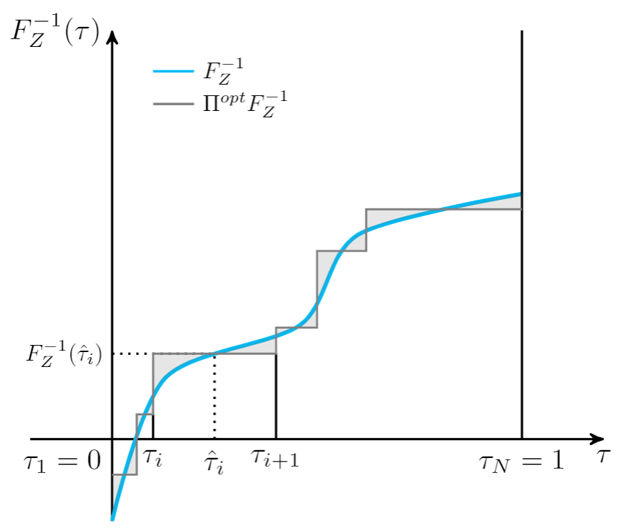
(a)

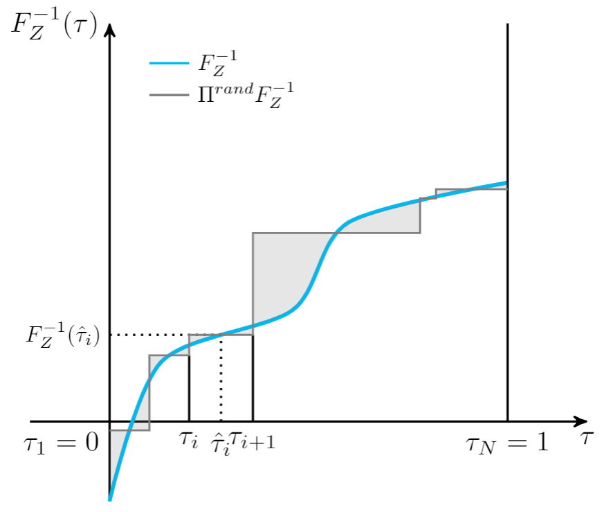
(b)

Figure 1: Two approximations of the same quantile function using different set of $\tau$ with $N=6$, the area of the shaded region is equal to the 1-Wasserstein error. (a) Finely-adjusted $\tau$ with minimized $W_{1}$ error. (b) Randomly chosen $\tau$ with larger $W_{1}$ error.

3.2 Training fraction proposal Network

To achieve minimal $1$-Wasserstein error, we start from fixing $\tau$ and finding the optimal corresponding quantile values $\theta$. In QR-DQN, Dabney et al. (2018a) gives an explicit form of $\theta$ to achieve the goal. We extend it to our setting:

Lemma 1.

(Dabney et al., 2018a) For any $\tau_{1},...\tau_{N-1}\in[0,1]$ satisfying $\tau_{i-1}<\tau_{i}$ for $i$, with $\tau_{1}=0$ and $\tau_{N}=1$, and cumulative distribution function $F$ with inverse $F^{-1}$, the set of $\theta$ minimizing Eq.(2) is given by

$$\theta_{i}=F^{-1}_{Z}(\frac{\tau_{i}+\tau_{i+1}}{2})$$ (3)

We can now substitute $\theta_{i}$ in Eq.(2) with equation Eq.(3) and find the optimal condition for $\tau$ to minimize $W_{1}(Z,\tau)$. For simplicity, we denote $\hat{\tau}_{i}=\frac{\tau_{i}+\tau_{i+1}}{2}$.

Proposition 1.

For any continuous quantile function $F^{-1}_{Z}$ that is non-decreasing, define the 1-Wasserstein loss of $F^{-1}_{Z}$ and $F^{-1,\tau}_{Z}$ by

$$W_{1}(Z,\tau)=\sum_{i=0}^{N-1}\int_{\tau_{i}}^{\tau_{i+1}}\left|F^{-1}_{Z}(\omega)-F^{-1}_{Z}(\hat{\tau}_{i})\right|d\omega.$$ (4)

$\frac{\partial W_{1}}{\partial\tau_{i}}$ is given by

$$\frac{\partial W_{1}}{\partial\tau_{i}}=2F^{-1}_{Z}(\tau_{i})-F^{-1}_{Z}(\hat{\tau}_{i})-F^{-1}_{Z}(\hat{\tau}_{i-1}),$$ (5)

$\forall i\in(0,N)$.

Further more, $\forall\tau_{i-1},\;\tau_{i+1}\in[0,1],\;\tau_{i-1}<\tau_{i+1},\;\exists\tau_{i}\in(\tau_{i-1},\tau_{i+1})\;s.t.\;\frac{\partial W_{1}}{\partial\tau_{i}}=0$.

Proof of proposition 1 is given in the appendix. While computing $W_{1}$ without bias is usually impractical, equation 5 provides us with a way to minimize $W_{1}$ without computing it. Let $w_{1}$ be the parameters of the fraction proposal network $P$, for an arbitrary quantile function $F_{Z}^{-1}$, we can minimize $W_{1}$ by iteratively applying gradients descent to $w_{1}$ according to Eq.(5) and convergence is guaranteed. As the true quantile function $F^{-1}_{Z}$ is unknown to us in practice, we use the quantile value network $F^{-1}_{Z,w_{2}}$ with parameters $w_{2}$ for current state and action as true quantile function.

The expected return, also known as action-value based on FQF is then given by

$$Q(x,a)=\sum_{i=0}^{N-1}(\tau_{i+1}-\tau_{i})F^{-1}_{Z,w_{2}}(\hat{\tau}_{i}),$$

where $\tau_{0}=0$ and $\tau_{N}=1$.

3.3 Training quantile value network

With the properly chosen probabilities, we combine quantile regression and distributional Bellman update on the optimized probabilities to train the quantile function. Consider $Z$ a random variable denoting the action-value at $(x_{t},a_{t})$ and $Z^{\prime}$ the action-value random variable at $(x_{t+1},a_{t+1})$, the weighted temporal difference (TD) error for two probabilities $\hat{\tau}_{i}$ and $\hat{\tau}_{j}$ is defined by

$$\delta_{ij}^{t}=r_{t}+\gamma F^{-1}_{Z^{\prime},w_{1}}(\hat{\tau}_{i})-F^{-1}_{Z,w_{1}}(\hat{\tau}_{j})$$ (6)

Quantile regression is used in QR-DQN and IQN to stochastically adjust the quantile estimates so as to minimize the Wasserstein distance to a target distribution. We follow QR-DQN and IQN where quantile value networks are trained by minimizing the Huber quantile regression loss (Huber, 1964), with threshold $\kappa$,

$$\rho_{\tau}^{\kappa}\left(\delta_{ij}\right)=\left|\tau-\mathbb{I}\left\{\delta_{ij}<0\right\}\right|\frac{\mathcal{L}_{\kappa}\left(\delta_{ij}\right)}{\kappa}\text{, with}$$

$$\mathcal{L}_{\kappa}\left(\delta_{ij}\right)=\left\{\begin{array}[]{ll}{\frac{1}{2}\delta_{ij}^{2},}&{\text{ if }\left|\delta_{ij}\right|\leq\kappa}\\ {\kappa\left(\left|\delta_{ij}\right|-\frac{1}{2}\kappa\right),}&{\text{ otherwise }}\end{array}\right.$$

The loss of the quantile value network is then given by

$$\mathcal{L}(x_{t},a_{t},r_{t},x_{t+1})=\frac{1}{N}\sum_{i=0}^{N-1}\sum_{j=0}^{N-1}\rho_{\hat{\tau}_{j}}^{\kappa}(\delta_{ij}^{t})$$ (7)

Note that $F^{-1}_{Z}$ and its Bellman target share the same proposed quantile fractions $\hat{\tau}$ to reduce computation.

We perform joint gradient update for $w_{1}$ and $w_{2}$, as illustrated in Algorithm 1.

Parameter : $N,\kappa$

Input: $x,a,r,x^{\prime},\gamma\in[0,1)$

// Compute proposed fractions for $x,a$

$\tau\leftarrow P_{w_{1}}(x,a)$;

// Compute proposed fractions for $x^{\prime},a^{\prime}$

for $a^{\prime}\in\mathcal{A}$ do

       $\tau^{a^{\prime}}\leftarrow P_{w_{1}}(x^{\prime},a^{\prime})$;

      

end for

// Compute greedy action

$Q(s^{\prime},a^{\prime})\leftarrow\sum_{i=0}^{N-1}(\tau^{a^{\prime}}_{i+1}-\tau^{a^{\prime}}_{i})F^{-1}_{Z^{\prime},w_{2}}(\hat{\tau}_{i}^{a^{\prime}})$;

$a^{*}\leftarrow\underset{a^{\prime}}{\mathrm{argmax}}Q(s^{\prime},a^{\prime})$;

// Compute $L$

for $0\leq i\leq N-1$ do

       for $0\leq j\leq N-1$ do

             $\delta_{ij}\leftarrow r+\gamma F^{-1}_{Z^{\prime},w_{2}}(\hat{\tau}_{i})-F^{-1}_{Z,w_{2}}(\hat{\tau}_{j})$

       end for

      

end for

$\mathcal{L}=\frac{1}{N}\sum_{i=0}^{N-1}\sum_{j=0}^{N-1}\rho_{\hat{\tau}_{j}}^{\kappa}(\delta_{ij})$;

// Compute $\frac{\partial W_{1}}{\partial\tau_{i}}$ for $i\in[1,N-1]$

$\frac{\partial W_{1}}{\partial\tau_{i}}=2F^{-1}_{Z,w_{2}}(\tau_{i})-F^{-1}_{Z,w_{2}}(\hat{\tau}_{i})-F^{-1}_{Z,w_{2}}(\hat{\tau}_{i-1})$;

Update $w_{1}$ with $\frac{\partial W_{1}}{\partial\tau_{i}}$; Update $w_{2}$ with $\nabla\mathcal{L}$;

Output: $Q$

Algorithm 1 FQF update

3.4 Implementation Details

Our fraction proposal network is represented by one fully-connected MLP layer. It takes the state embedding of original IQN as input and generates fraction proposal. Recall that in Proposition 1, we require $\tau_{i-1}<\tau_{i}$ and $\tau_{0}=0,\tau_{N}=1$. While it is feasible to have $\tau_{0}=0,\tau_{N}=1$ fixed and sort the output of $\tau_{w_{1}}$, the sort operation would make the network hard to train. A more reasonable and practical way would be to let the neural network automatically have the output sorted using cumulated softmax. Let $q\in\mathbb{R}^{N}$ denote the output of a softmax layer, we have $q_{i}\in(0,1),i\in[0,N-1]$ and $\sum_{i=0}^{N-1}q_{i}=1$. Let $\tau_{i}=\sum_{j=0}^{i-1}q_{j},i\in[0,N]$, then straightforwardly we have $\tau_{i}<\tau_{j}$ for $\forall i<j$ and $\tau_{0}=0,\tau_{N}=1$ in our fraction proposal network. Note that as $W_{1}$ is not computed, we can’t directly perform gradient descent for the fraction proposal network. Instead, we use the grad_ys argument in the tensorflow operator tf.gradients to assign $\frac{\partial W_{1}}{\partial\tau_{i}}$ to the optimizer. In addition, one can use entropy of $q$ as a regularization term $H(q)=-\sum_{i=0}^{N-1}q_{i}\log q_{i}$ to prevent the distribution from degenerating into a deterministic one.

We borrow the idea of implicit representations from IQN to our quantile value network. To be specific, we compute the embedding of $\tau$, denoted by $\phi(\tau)$, with

$$\phi_{j}(\tau):=\operatorname{ReLU}\left(\sum_{i=0}^{n-1}\cos(i\pi\tau)w_{ij}+b_{j}\right),$$

where $w_{ij}$ and $b_{j}$ are network parameters. We then compute the element-wise (Hadamard) product of state feature $\psi(x)$ and embedding $\phi(\tau)$. Let $\odot$ denote element-wise product, the quantile values are given by $F^{-1}_{Z}(\tau)\approx F^{-1}_{Z,w_{2}}(\psi(x)\odot\phi(\tau))$.

In IQN, after the set of $\tau$ is sampled from a uniform distribution, instead of using differences between $\tau$ as probabilities of the quantiles, the mean of the quantile values is used to compute action-value $Q$. While in expectation, $Q=\sum_{i=0}^{N-1}(\tau_{i+1}-\tau_{i})F^{-1}_{Z}(\frac{\tau_{i}+\tau_{i+1}}{2})$ with $\tau_{0}=0,\tau_{N}=1$ and $Q=\frac{1}{N}\sum_{i=1}^{N}F^{-1}_{Z}(\tau_{i})$ are equal, we use the former one to consist with our projection operation.

4 Experiments

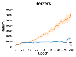
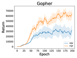
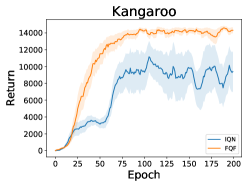
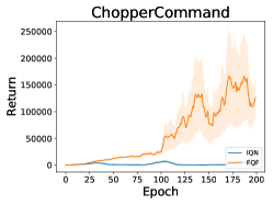
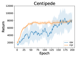
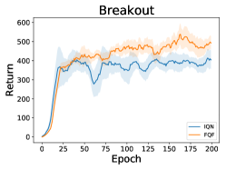
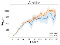
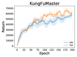
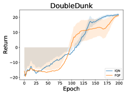
Figure 2: Performance comparison with IQN. Each training curve is averaged by 3 seeds. The training curves are smoothed with a moving average of 10 to improve readability.

We test our algorithm on the Atari games from Arcade Learning Environment (ALE) Bellemare et al. (2013). We select the most relative algorithm to ours, IQN (Dabney et al., 2018a), as baseline, and compare FQF with QR-DQN (Dabney et al., 2018b), C51 (Bellemare et al., 2017), prioritized experience replay (Schaul et al., 2016) and Rainbow (Hessel et al., 2018), the current state-of-art that combines the advantages of several RL algorithms including distributional RL. The baseline algorithm is implemented by Castro et al. (2018) in the Dopamine framework, with slightly lower performance than reported in IQN. We implement FQF based on the Dopamine framework. Unfortunately, we fail to test our algorithm on Surround and Defender as Surround is not supported by the Dopamine framework and scores of Defender is unreliable in Dopamine. Following the common practice (Van Hasselt et al., 2016), we use the 30-noop evaluation settings to align with previous works. Results of FQF and IQN using sticky action for evaluation proposed by Machado et al. (2018) are also provided in the appendix. In all, the algorithms are tested on 55 Atari games.

Our hyper-parameter setting is aligned with IQN for fair comparison. The number of $\tau$ for FQF is 32. The weights of the fraction proposal network are initialized so that initial probabilities are uniform as in QR-DQN, also the learning rates are relatively small compared with the quantile value network to keep the probabilities relatively stable while training. We run all agents with 200 million frames. At the training stage, we use $\epsilon$-greedy with $\epsilon=0.01$. For each evaluation stage, we test the agent for 0.125 million frames with $\epsilon=0.001$. For each algorithm we run 3 random seeds. All experiments are performed on NVIDIA Tesla V100 16GB graphics cards.

	Mean	Median	>Human	>DQN
DQN	221%	79%	24	0
PRIOR.	580%	124%	39	48
C51	701%	178%	40	50
RAINBOW	1213%	227%	42	52
QR-DQN	902%	193%	41	54
IQN	1112%	218%	39	54
FQF	1426%	272%	44	54

Table 1: Mean and median scores across 55 Atari 2600 games, measured as percentages of human baseline. Scores are averages over 3 seeds.

Table 1 compares the mean and median human normalized scores across 55 Atari games with up to 30 random no-op starts, and the full score table is provided in the Appendix. It shows that FQF outperforms all existing distributional RL algorithms, including Rainbow (Hessel et al., 2018) that combines C51 with prioritized replay, and n-step updates. We also set a new record on the number of games where non-distributed RL agent performs better than human.

Figure 2 shows the training curves of several Atari games. Even on games where FQF and IQN have similar performance such as Centipede , FQF is generally much faster thanks to self-adjusting fractions.

However, one side effect of the full parameterization in FQF is that the training speed is decreased. With same settings, FQF is roughly 20% slower than IQN due to the additional fraction proposal network. As the number of $\tau$ increases, FQF slows down significantly while IQN’s training speed is not sensitive to the number of $\tau$ samples.

5 Discussion and Conclusions

Based on previous works of distributional RL, we propose a more general complete approximation of the return distribution. Compared with previous distributional RL algorithms, FQF focuses not only on learning the target, e.g. probabilities for C51, quantile values for QR-DQN and IQN, but also which target to learn, i.e quantile fraction. This allows FQF to learn a better approximation of the true distribution under restrictions of network capacity. Experiment result shows that FQF does achieve significant improvement.

There are some open questions we are yet unable to address in this paper. We will have some discussions here. First, does the $1$-Wasserstein error converge to its minimal value when the quantile function is not fixed? We cannot guarantee convergence of the fraction proposal network in deep neural networks where we involve quantile regression and Bellman update. Second, though we empirically believe so, does the contraction mapping result for fixed probabilities given by Dabney et al. (2018b) also apply on self-adjusting probabilities? Third, while FQF does provide potentially better distribution approximation with same amount of fractions, how will a better approximated distribution affect agent’s policy and how will it affect the training process? More generally, how important is quantile fraction selection during training?

As for future work, we believe that studying the trained quantile fractions will provide intriguing results. Such as how sensitive are the quantile fractions to state and action, and that how the quantile fractions will evolve in a single run. Also, the combination of distributional RL and DDPG in D4PG (Barth-Maron et al., 2018) showed that distributional RL can also be extended to continuous control settings. Extending our algorithm to continuous settings is another interesting topic. Furthermore, in our algorithm we adopted the concept of selecting the best target to learn. Can this intuition be applied to areas other than RL?

Finally, we also noticed that most of the games we fail to reach human-level performance involves complex rules that requires exploration based policies, such as Montezuma Revenge and Venture. Integrating distributional RL will be another potential direction as in (Tang and Agrawal, 2018). In general, we believe that our algorithm can be viewed as a natural extension of existing distributional RL algorithms, and that distributional RL may integrate greatly with other algorithms to reach higher performance.

Appendix

Proof for proposition 1

See 1

Proof.

Note that $F^{-1}_{Z}$ is non-decreasing. We have

$$\begin{split}\frac{\partial W_{1}}{\partial\tau_{i}}=&\frac{\partial}{\partial\tau_{i}}(\int_{\tau_{i-1}}^{\tau_{i}}\left|F^{-1}_{Z}(\omega)-F^{-1}_{Z}(\hat{\tau}_{i-1})\right|d\omega+\int_{\tau_{i}}^{\tau_{i+1}}\left|F^{-1}_{Z}(\omega)-F^{-1}_{Z}(\hat{\tau}_{i})\right|d\omega)\\ =&\frac{\partial}{\partial\tau_{i}}(\int_{\tau_{i-1}}^{\hat{\tau}_{i-1}}F^{-1}_{Z}(\hat{\tau}_{i-1})-F^{-1}_{Z}(\omega)d\omega+\int_{\hat{\tau}_{i-1}}^{\tau_{i}}F^{-1}_{Z}(\omega)-F^{-1}_{Z}(\hat{\tau}_{i-1})d\omega+\\ &\int_{\tau_{i}}^{\tau_{i+1}}\left|F^{-1}_{Z}(\omega)-F^{-1}_{Z}(\hat{\tau}_{i})\right|d\omega))\\ =&\frac{\tau_{i}-\tau_{i-1}}{4}\frac{\partial}{\partial\tau_{i}}F^{-1}_{Z}(\hat{\tau}_{i-1})+F^{-1}_{Z}(\tau_{i})-F^{-1}_{Z}(\hat{\tau}_{i-1})-\frac{\tau_{i}-\tau_{i-1}}{4}\frac{\partial}{\partial\tau_{i}}F^{-1}_{Z}(\hat{\tau}_{i-1})+\\ &\frac{\partial}{\partial\tau_{i}}(\int_{\tau_{i}}^{\tau_{i+1}}\left|F^{-1}_{Z}(\omega)-F^{-1}_{Z}(\hat{\tau}_{i})\right|d\omega))\\ =&F^{-1}_{Z}(\tau_{i})-F^{-1}_{Z}(\hat{\tau}_{i-1})+\frac{\partial}{\partial\tau_{i}}(\int_{\tau_{i}}^{\tau_{i+1}}\left|F^{-1}_{Z}(\omega)-F^{-1}_{Z}(\hat{\tau}_{i})\right|d\omega))\\ =&F^{-1}_{Z}(\tau_{i})-F^{-1}_{Z}(\hat{\tau}_{i-1})+F^{-1}_{Z}(\tau_{i})-F^{-1}_{Z}(\hat{\tau}_{i})\\ =&2F^{-1}_{Z}(\tau_{i})-F^{-1}_{Z}(\hat{\tau}_{i-1})-F^{-1}_{Z}(\hat{\tau}_{i})\end{split}$$

As $F^{-1}_{Z}$ is non-decreasing we have $\frac{\partial W_{1}}{\partial\tau_{i}}|_{\tau_{i}=\tau_{i-1}}\leq 0$ and $\frac{\partial W_{1}}{\partial\tau_{i}}|_{\tau_{i}=\tau_{i+1}}\geq 0$. Recall that $F^{-1}_{Z}$ is continuous, so $\exists\tau_{i}\in(\tau_{i-1},\tau_{i+1})\ s.t.\ \frac{\partial W_{1}}{\partial\tau_{i}}=0$. ∎

Hyper-parameter sheet

Hyper-parameter	IQN	FQF
Learning rate	0.00005	0.00005
Optimizer	Adam	Adam
Batch size	32	32
Discount factor	0.99	0.99
Fraction proposal network learning rate	None	2.5e-9
Fraction proposal network optimizer	None	RMSProp

Table 2: hyper-parameter list

We sweep the learning rate of fraction proposal network among (0, 2.5e-5) and finally fix this learning rate as 2.5e-9. For the training of fraction proposal network, we use RMSProp optimizer. Note that though the fraction proposal network takes the state embedding of original IQN as input, we only apply gradient to our new introduced parameter and do not back-propagate the gradient to the convolution layers.

Approximation demonstration

To demonstrate how FQF provides a better quantile function approximation, figure 3 provides plots of a toy case with different distributional RL algorithm’s approximation of a known quantile function, from which we can see how quantile fraction selection affects distribution approximation.

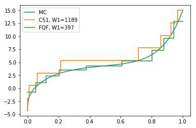
(a)

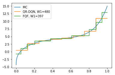
(b)

Figure 3: Demonstration of quantile function approximation on a toy case. $W_{1}$ denotes 1-Wasserstein distance between the approximated function and the one obtained through MC method.

Varying number of quantile fractions

Table 3 gives mean scores of FQF and IQN over 6 Atari games, using different number of quantile fractions, i.e. $N$. For IQN, the selection of $N^{\prime}$ is based on the highest score of each column given in Figure 2 of [Dabney et al., 2018a].

	N=8	N=32	N=64
IQN	60.2	91.5	64.4
FQF	83.2	124.6	69.5

Table 3: Mean scores across 6 Atari 2600 games, measured as percentages of human baseline. Scores are averages over 3 seeds.

Intuitively, the advantage of trained quantile fractions compared to random ones will be more observable at smaller $N$. At larger $N$ when both trained quantile fractions and random ones are densely distributed over $[0,1]$, the differences between FQF and IQN becomes negligible. However from table 3 we see that even at large $N$, FQF performs slightly better than IQN.

Visualizing proposed quantile fraction

In figure 4, we select a half-trained Kungfu Master agent with $N=8$ to provide a case study of FQF. The reason why we choose a half-trained agent instead of a fully-trained agent is so that the distribution of $Q$ is not a deterministic one. Note that theoretically the quantile function should be non-decreasing, however from the example we can see that the learned quantile function might not always follow this property, and this phenomenon further motivates a quite interesting future work that leverages the non-decreasing property as prior knowledge for quantile function learning. The figure shows how the interval between proposed quantile fractions (i.e., the output of the softmax layer that sums to 1. See Section 3.4 for details) vary during a single run.

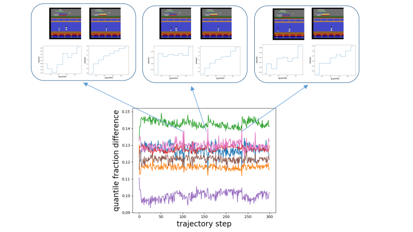
Figure 4: Interval between adjacent proposed quantile fractions for states at each time step in a single run. Different colors refer to different adjacent fractions’ intervals, e.g. green curve refers to $\tau_{2}-\tau_{1}$.

Whenever there appears an enemy behind the character, we see a spike in the fraction interval, indicating that proposed fraction is very different from that of following states without enemies. This suggests that the fraction proposal network is indeed state dependent and is able to provide different quantile fractions accordingly.

ALE Scores

GAMES	RANDOM	HUMAN	DQN	PRIOR.DUEL.	QR-DQN	IQN	FQF
Alien	227.8	7127.7	1620.0	3941.0	4871.0	7022.0	16754.6
Amidar	5.8	1719.5	978.0	2296.8	1641.0	2946.0	3165.3
Assault	222.4	742.0	4280.4	11477.0	22012.0	29091.0	23020.1
Asterix	210.0	8503.3	4359.0	375080.0	261025.0	342016.0	578388.5
Asteroids	719.1	47388.7	1364.5	1192.7	4226.0	2898.0	4553.0
Atlantis	12850.0	29028.1	279987.0	395762.0	971850.0	978200.0	957920.0
BankHeist	14.2	753.1	455.0	1503.1	1249.0	1416.0	1259.1
BattleZone	2360.0	37187.5	29900.0	35520.0	39268.0	42244.0	87928.6
BeamRider	363.9	16926.5	8627.5	30276.5	34821.0	42776.0	37106.6
Berzerk	123.7	2630.4	585.6	3409.0	3117.0	1053.0	12422.2
Bowling	23.1	160.7	50.4	46.7	77.2	86.5	102.3
Boxing	0.1	12.1	88.0	98.9	99.9	99.8	98.0
Breakout	1.7	30.5	385.5	366.0	742.0	734.0	854.2
Centipede	2090.9	12017.0	4657.7	7687.5	12447.0	11561.0	11526.0
ChopperCommand	811.0	7387.8	6126.0	13185.0	14667.0	16836.0	876460.0
CrazyClimber	10780.5	35829.4	110763.0	162224.0	161196.0	179082.0	223470.6
DemonAttack	152.1	1971.0	12149.4	72878.6	121551.0	128580.0	131697.0
DoubleDunk	-18.6	-16.4	-6.6	-12.5	21.9	5.6	22.9
Enduro	0.0	860.5	729.0	2306.4	2355.0	2359.0	2370.8
FishingDerby	-91.7	-38.7	-4.9	41.3	39.0	33.8	52.7
Freeway	0.0	29.6	30.8	33.0	34.0	34.0	33.7
Frostbite	65.2	4334.7	797.4	7413.0	4384.0	4324.0	16472.9
Gopher	257.6	2412.5	8777.4	104368.2	113585.0	118365.0	121144.0
Gravitar	173.0	3351.4	473.0	238.0	995.0	911.0	1406.0
Hero	1027.0	30826.4	20437.8	21036.5	21395.0	28386.0	30926.2
IceHockey	-11.2	0.9	-1.9	-0.4	-1.7	0.2	17.3
Jamesbond	29.0	302.8	768.5	812.0	4703.0	35108.0	87291.7
Kangaroo	52.0	3035.0	7259.0	1792.0	15356.0	15487.0	15400.0
Krull	1598.0	2665.5	8422.3	10374.0	11447.0	10707.0	10706.8
KungFuMaster	258.5	22736.3	26059.0	48375.0	76642.0	73512.0	111138.5
MontezumaRevenge	0.0	4753.3	0.0	0.0	0.0	0.0	0.0
MsPacman	307.3	6951.6	3085.6	3327.3	5821.0	6349.0	7631.9
NameThisGame	2292.3	8049.0	8207.8	15572.5	21890.0	22682.0	16989.4
Phoenix	761.4	7242.6	8485.2	70324.3	16585.0	56599.0	174077.5
Pitfall	-229.4	6463.7	-286.1	0.0	0.0	0.0	0.0
Pong	-20.7	14.6	19.5	20.9	21.0	21.0	21.0
PrivateEye	24.9	69571.3	146.7	206.0	350.0	200.0	140.1
Qbert	163.9	13455.0	13117.3	18760.3	572510.0	25750.0	27524.4
Riverraid	1338.5	17118.0	7377.6	20607.6	17571.0	17765.0	23560.7
RoadRunner	11.5	7845.0	39544.0	62151.0	64262.0	57900.0	58072.7
Robotank	2.2	11.9	63.9	27.5	59.4	62.5	75.7
Seaquest	68.4	42054.7	5860.6	931.6	8268.0	30140.0	29383.3
Skiing	-17098.1	-4336.9	-13062.3	-19949.9	-9324.0	-9289.0	-9085.3
Solaris	1236.3	12326.7	3482.8	133.4	6740.0	8007.0	6906.7
SpaceInvaders	148.0	1668.7	1692.3	15311.5	20972.0	28888.0	46498.3
StarGunner	664.0	10250.0	54282.0	125117.0	77495.0	74677.0	131981.2
Tennis	-23.8	-9.3	12.2	0.0	23.6	23.6	22.6
TimePilot	3568.0	5229.2	4870.0	7553.0	10345.0	12236.0	14995.2
Tutankham	11.4	167.6	68.1	245.9	297.0	293.0	309.2
UpNDown	533.4	11693.2	9989.9	33879.1	71260.0	88148.0	75474.4
Venture	0.0	1187.5	163.0	48.0	43.9	1318.0	1112
VideoPinball	16256.9	17667.9	196760.4	479197.0	705662.0	698045.0	799155.6
WizardOfWor	563.5	4756.5	2704.0	12352.0	25061.0	31190.0	44782.6
YarsRevenge	3092.9	54576.9	18098.9	69618.1	26447.0	28379.0	27691.2
Zaxxon	32.5	9173.3	5363.0	13886.0	13113.0	21772.0	15179.5

Table 4: Raw scores for a single seed across all games, starting with 30 no-op actions.

To align with previous works, the scores are evaluated under 30 no-op setting. As the sticky action evaluation setting proposed by Machado et al. [2018] is generally considered more meaningful in the RL community, we will add results under sticky-action evaluation setting after the conference.

References

- Barth-Maron et al. [2018] Gabriel Barth-Maron, Matthew W Hoffman, David Budden, Will Dabney, Dan Horgan, Alistair Muldal, Nicolas Heess, and Timothy Lillicrap. Distributed distributional deterministic policy gradients. International Conference on Learning Representations, 2018.
- Bellemare et al. [2013] Marc G Bellemare, Yavar Naddaf, Joel Veness, and Michael Bowling. The arcade learning environment: An evaluation platform for general agents. Journal of Artificial Intelligence Research, 47:253–279, 2013.
- Bellemare et al. [2017] Marc G Bellemare, Will Dabney, and Rémi Munos. A distributional perspective on reinforcement learning. In Proceedings of the 34th International Conference on Machine Learning-Volume 70, pages 449–458. JMLR. org, 2017.
- Bellman [1957] Richard Bellman. Dynamic Programming. Princeton University Press, Princeton, NJ, USA, 1 edition, 1957.
- Castro et al. [2018] Pablo Samuel Castro, Subhodeep Moitra, Carles Gelada, Saurabh Kumar, and Marc G. Bellemare. Dopamine: A Research Framework for Deep Reinforcement Learning. 2018. URL http://arxiv.org/abs/1812.06110.
- Dabney et al. [2018a] Will Dabney, Georg Ostrovski, David Silver, and Remi Munos. Implicit quantile networks for distributional reinforcement learning. In International Conference on Machine Learning, pages 1104–1113, 2018a.
- Dabney et al. [2018b] Will Dabney, Mark Rowland, Marc G Bellemare, and Rémi Munos. Distributional reinforcement learning with quantile regression. In Thirty-Second AAAI Conference on Artificial Intelligence, 2018b.
- Hessel et al. [2018] Matteo Hessel, Joseph Modayil, Hado Van Hasselt, Tom Schaul, Georg Ostrovski, Will Dabney, Dan Horgan, Bilal Piot, Mohammad Azar, and David Silver. Rainbow: Combining improvements in deep reinforcement learning. In Thirty-Second AAAI Conference on Artificial Intelligence, 2018.
- Huber [1964] Peter J. Huber. Robust estimation of a location parameter. Annals of Mathematical Statistics, 35(1):73–101, March 1964. ISSN 0003-4851. doi: 10.1214/aoms/1177703732.
- Jaquette et al. [1973] Stratton C Jaquette et al. Markov decision processes with a new optimality criterion: Discrete time. The Annals of Statistics, 1(3):496–505, 1973.
- Kapturowski et al. [2018] Steven Kapturowski, Georg Ostrovski, John Quan, Remi Munos, and Will Dabney. Recurrent experience replay in distributed reinforcement learning. 2018.
- Machado et al. [2018] Marlos C Machado, Marc G Bellemare, Erik Talvitie, Joel Veness, Matthew Hausknecht, and Michael Bowling. Revisiting the arcade learning environment: Evaluation protocols and open problems for general agents. Journal of Artificial Intelligence Research, 61:523–562, 2018.
- Mnih et al. [2015] Volodymyr Mnih, Koray Kavukcuoglu, David Silver, Andrei A Rusu, Joel Veness, Marc G Bellemare, Alex Graves, Martin Riedmiller, Andreas K Fidjeland, Georg Ostrovski, et al. Human-level control through deep reinforcement learning. Nature, 518(7540):529, 2015.
- Morimura et al. [2010] Tetsuro Morimura, Masashi Sugiyama, Hisashi Kashima, Hirotaka Hachiya, and Toshiyuki Tanaka. Nonparametric return distribution approximation for reinforcement learning. In Proceedings of the 27th International Conference on Machine Learning (ICML-10), pages 799–806, 2010.
- Müller [1997] Alfred Müller. Integral probability metrics and their generating classes of functions. Advances in Applied Probability, 29(2):429–443, 1997.
- Puterman [1994] Martin L. Puterman. Markov Decision Processes: Discrete Stochastic Dynamic Programming. John Wiley & Sons, Inc., New York, NY, USA, 1st edition, 1994. ISBN 0471619779.
- Rowland et al. [2018] Mark Rowland, Marc Bellemare, Will Dabney, Remi Munos, and Yee Whye Teh. An analysis of categorical distributional reinforcement learning. In International Conference on Artificial Intelligence and Statistics, pages 29–37, 2018.
- Schaul et al. [2016] Tom Schaul, John Quan, Ioannis Antonoglou, and David Silver. Prioritized experience replay. International Conference on Learning Representations, abs/1511.05952, 2016.
- Sobel [1982] Matthew J Sobel. The variance of discounted markov decision processes. Journal of Applied Probability, 19(4):794–802, 1982.
- Sutton [1988] Richard S Sutton. Learning to predict by the methods of temporal differences. Machine learning, 3(1):9–44, 1988.
- Tang and Agrawal [2018] Yunhao Tang and Shipra Agrawal. Exploration by distributional reinforcement learning. In Proceedings of the 27th International Joint Conference on Artificial Intelligence, pages 2710–2716. AAAI Press, 2018.
- Van Hasselt et al. [2016] Hado Van Hasselt, Arthur Guez, and David Silver. Deep reinforcement learning with double q-learning. In Thirtieth AAAI Conference on Artificial Intelligence, 2016.
- Wang et al. [2016] Ziyu Wang, Tom Schaul, Matteo Hessel, Hado Hasselt, Marc Lanctot, and Nando Freitas. Dueling network architectures for deep reinforcement learning. In International Conference on Machine Learning, pages 1995–2003, 2016.
- Watkins [1989] Christopher John Cornish Hellaby Watkins. Learning from delayed rewards. 1989.
- White [1988] DJ White. Mean, variance, and probabilistic criteria in finite markov decision processes: a review. Journal of Optimization Theory and Applications, 56(1):1–29, 1988.