Informed reversible jump algorithms

Abstract

Incorporating information about the target distribution in proposal mechanisms generally produces efficient Markov chain Monte Carlo algorithms (or at least, algorithms that are more efficient than uninformed counterparts). For instance, it has proved successful to incorporate gradient information in fixed-dimensional algorithms, as seen with algorithms such as Hamiltonian Monte Carlo. In trans-dimensional algorithms, Green (2003) recommended to sample the parameter proposals during model switches from normal distributions with informative means and covariance matrices. These proposal distributions can be viewed as asymptotic approximations to the parameter distributions, where the limit is with regard to the sample size. Models are typically proposed using uninformed uniform distributions. In this paper, we build on the approach of Zanella (2020) for discrete spaces to incorporate information about neighbouring models. We rely on approximations to posterior model probabilities that are asymptotically exact. We prove that, in some scenarios, the samplers combining this approach with that of Green (2003) behave like ideal ones that use the exact model probabilities and sample from the correct parameter distributions, in the large-sample regime. We show that the implementation of the proposed samplers is straightforward in some cases. The methodology is applied to a real-data example. The code is available online.

¹Department of Mathematics and Statistics, Université de Montréal, Canada.

Keywords: Bayesian statistics; large-sample asymptotics; Markov chain Monte Carlo methods; model averaging; model selection; trans-dimensional samplers; variable selection; weak convergence.

1 Introduction

1.1 Reversible jump algorithms

Reversible jump (RJ, Green (1995)) algorithms are Markov chain Monte Carlo (MCMC) methods that one uses to sample from a target distribution $\pi(\,\cdot\,,\cdot\mid\mathbf{D}_{n})$ defined on a union of sets $\bigcup_{k\in\mathcal{K}}\{k\}\times\mathbb{R}^{d_{k}}$, $\mathcal{K}$ being a countable set and $d_{k}$ positive integers. This distribution corresponds in Bayesian statistics to a joint posterior distribution of a model indicator $K\in\mathcal{K}$ and the parameters of Model $K$, denoted by $\mathbf{X}_{K}\in\mathbb{R}^{d_{K}}$, given $\mathbf{D}_{n}$, a data sample of size $n$. Such a posterior distribution allows to jointly infer about $(K,\mathbf{X}_{K})$, or in other words, to simultaneously achieve model selection/averaging (Hoeting et al., 1999) and parameter estimation. In the following, we assume for simplicity that the parameters of all models are continuous random variables. Again for simplicity, we will abuse notation by also using $\pi(\,\cdot\,,\cdot\mid\mathbf{D}_{n})$ to denote the joint posterior density with respect to a product of the counting and Lebesgue measures. We will use $\pi(\,\cdot\,\mid\mathbf{D}_{n})$ and $\pi(\,\cdot\,\mid k,\mathbf{D}_{n})$ to denote the marginal posterior probability mass function (PMF) of $K$ and conditional posterior distribution/density of $\mathbf{X}_{K}$ given that $K=k$, respectively. Note that in this paper, we assume that $\mathcal{K}$ is defined such that $\pi(k\mid\mathbf{D}_{n})>0$ for all $k$.

The variable $K\in\mathcal{K}$ can take different forms in practice. In mixture modelling (Richardson and Green, 1997), $K$ is the number of components and $\mathcal{K}$ is a subset of the positive integers and defines a sequence of nested models, i.e. Model 1 is nested in Model 2 which is nested in Model 3, and so on. Often there is no such “ordering” between the models. This is for instance the case in variable selection. In this framework, $K$ is a vector of $0$’s and $1$’s indicating which covariates are included in a model, and for instance, Model $k_{0}=(1,1,1,0,0,1,0,\ldots,0)$ is the model with covariates 1, 2, 3 and 6 (as in Figure 1 below); $\mathcal{K}$ is thus a collection of such vectors. A RJ algorithm explores both the model space and the parameter spaces. We focus in this paper on the case where $\mathcal{K}$ does not define a sequence of nested models. When $\mathcal{K}$ defines a sequence of nested models, $K$ can be recoded as an ordinal discrete variable as above and this case has been recently studied by Gagnon and Doucet (2021) who proposed efficient non-reversible trans-dimensional samplers.

The proposal mechanism in a RJ algorithm can be outlined as follows: given a current state of the Markov chain $(k,\mathbf{x}_{k})$, the algorithm first proposes a model, say Model $k^{\prime}$, by using a PMF $g(k,\cdot\,)$ and then parameter values for this model by applying a diffeomorphism $\mathcal{D}_{k\mapsto k^{\prime}}$ to $\mathbf{x}_{k}$ and auxiliary variables $\mathbf{u}_{k\mapsto k^{\prime}}\sim q_{k\mapsto k^{\prime}}$, yielding the parameter proposal $\mathbf{y}_{k^{\prime}}$ and another vector of auxiliary variables $\mathbf{u}_{k^{\prime}\mapsto k}$. The proposal is accepted, meaning that the next state of the Markov chain is $(k^{\prime},\mathbf{y}_{k^{\prime}})$, with probability (assuming that the current state has positive density under the target):

$$\alpha_{\text{RJ}}((k,\mathbf{x}_{k}),(k^{\prime},\mathbf{y}_{k^{\prime}})):=1\wedge\frac{\pi(k^{\prime},\mathbf{y}_{k^{\prime}}\mid\mathbf{D}_{n})\,g(k^{\prime},k)\,q_{k^{\prime}\mapsto k}(\mathbf{u}_{k^{\prime}\mapsto k})}{\pi(k,\mathbf{x}_{k}\mid\mathbf{D}_{n})\,g(k,k^{\prime})\,q_{k\mapsto k^{\prime}}(\mathbf{u}_{k\mapsto k^{\prime}})\,|J_{\mathcal{D}_{k\mapsto k^{\prime}}}(\mathbf{x}_{k},\mathbf{u}_{k\mapsto k^{\prime}})|^{-1}},$$ (1)

where $x\wedge y:=\min(x,y)$ and $|J_{\mathcal{D}_{k\mapsto k^{\prime}}}(\mathbf{x}_{k},\mathbf{u}_{k\mapsto k^{\prime}})|$ is the absolute value of the determinant of the Jacobian matrix of the function $\mathcal{D}_{k\mapsto k^{\prime}}$. If the proposal is rejected, the chain remains at the same state $(k,\mathbf{x}_{k})$. Recall that a diffeomorphism is a differentiable map having a differentiable inverse and note that we abused notation by using $q_{k\mapsto k^{\prime}}$ to denote both the distribution and the probability density function (PDF) of $\mathbf{u}_{k\mapsto k^{\prime}}$. The notation $k\mapsto k^{\prime}$ in subscript is used to highlight a dependence on the model transition that is proposed, which is from Model $k$ to Model $k^{\prime}$. In the particular case where $k^{\prime}=k$, we say that a parameter update is proposed; otherwise, we say that a model switch is proposed. Model $k^{\prime}$ is reachable from Model $k$ if it belongs to the support of $g(k,\cdot\,)$ which is considered in this paper to be the neighbourhood of Model $k$, denoted by $\mathbf{N}(k)$.

In trans-dimensional samplers, the neighbourhoods are usually formed of the “closest” models. The notion of “proximity” is often natural, making these closest models straightforward to identify. For instance, in Section 4 we apply the proposed methodology in a variable-selection example and the closest models are those with an additional and one less covariates, to which the current model is added. In this paper, we consider that Model $k$ belongs to the support of $g(k,\cdot\,)$ for all $k$; this will be seen to be useful when the posterior model PMF concentrates.

Algorithm 1 presents a general RJ.

Algorithm 1 RJ

1. Sample $k^{\prime}\sim g(k,\cdot\,)$, $\mathbf{u}_{k\mapsto k^{\prime}}\sim q_{k\mapsto k^{\prime}}$ and $u\sim\mathcal{U}[0,1]$.

2. Apply $\mathcal{D}_{k\mapsto k^{\prime}}(\mathbf{x}_{k},\mathbf{u}_{k\mapsto k^{\prime}})=(\mathbf{y}_{k^{\prime}},\mathbf{u}_{k^{\prime}\mapsto k})$.

3. If $u\leq\alpha_{\text{RJ}}((k,\mathbf{x}_{k}),(k^{\prime},\mathbf{y}_{k^{\prime}}))$, set the next state of the chain to $(k^{\prime},\mathbf{y}_{k^{\prime}})$. Otherwise, set it to $(k,\mathbf{x}_{k})$.

4. Go to Step 1.

Looping over the steps described in Algorithm 1 produces Markov chains that are reversible with respect to the target distribution $\pi(\,\cdot\,,\cdot\mid\mathbf{D}_{n})$. If the chains are in addition irreducible and aperiodic, then they are ergodic (Tierney, 1994), which guarantees, among others, that the law of large numbers holds, implying that ergodic averages are approximations to expectations under $\pi(\,\cdot\,,\cdot\mid\mathbf{D}_{n})$.

1.2 Problems with RJ

Algorithm 1 takes as inputs: an initial state $(k,\mathbf{x}_{k})$, a total number of iterations, a PMF $g(k,\cdot\,)$ for each Model $k$, and functions $q_{k\mapsto k^{\prime}}$ and $\mathcal{D}_{k\mapsto k^{\prime}}$ for each pair $(k,k^{\prime})$ with Model $k^{\prime}$ being reachable from Model $k$. Implementing RJ is well known for being a difficult task considering the large number of functions that need to be specified and the often lack of intuition about how one should achieve their specification, the latter being especially true for functions involved in model switches. Significant amount of work has been carried out to address the specification of the functions $q_{k\mapsto k^{\prime}}$ and $\mathcal{D}_{k\mapsto k^{\prime}}$ involved in model switches in a principled and informed way; see, e.g., Green (2003) and Brooks et al. (2003). The approaches of these authors are arguably the most popular. Their objective is the following: given $\mathbf{x}_{k}\sim\pi(\,\cdot\mid k,\mathbf{D}_{n})$, we want to identify $q_{k\mapsto k^{\prime}},q_{k^{\prime}\mapsto k}$ and $\mathcal{D}_{k\mapsto k^{\prime}}$ such that applying the transformation $\mathcal{D}_{k\mapsto k^{\prime}}$ to $(\mathbf{x}_{k},\mathbf{u}_{k\mapsto k^{\prime}})\sim\pi(\,\cdot\mid k,\mathbf{D}_{n})\otimes q_{k\mapsto k^{\prime}}$ leads to $(\mathbf{y}_{k^{\prime}},\mathbf{u}_{k^{\prime}\mapsto k})\sim\pi(\,\cdot\mid k^{\prime},\mathbf{D}_{n})\otimes q_{k^{\prime}\mapsto k}$ (at least approximatively). They essentially look for a way to sample from the conditional distributions $\pi(\,\cdot\mid k^{\prime},\mathbf{D}_{n})$, in this constrained framework. This in turn aims at increasing the acceptance probability $\alpha_{\text{RJ}}$ defined in (1) towards

$$\alpha_{\text{MH}}(k,k^{\prime}):=1\wedge\frac{\pi(k^{\prime}\mid\mathbf{D}_{n})\,g(k^{\prime},k)}{\pi(k\mid\mathbf{D}_{n})\,g(k,k^{\prime})},$$ (2)

which corresponds to the acceptance probability in a Metropolis–Hastings (MH, Metropolis et al. (1953) and Hastings (1970)) algorithm targeting the PMF $\pi(\,\cdot\mid\mathbf{D}_{n})$. The approach of Green (2003), for instance, proceeds as if the conditional distributions $\pi(\,\cdot\mid k^{\prime},\mathbf{D}_{n})$ were normal.

Notwithstanding the merit of this objective, it is to be noticed that, even when it is achieved, “half” of the work for maximizing $\alpha_{\text{RJ}}$ is done because, as shown in Figure 1, poor models may be proposed more often than they should be if $g$ is not well designed, leading to smaller acceptance rates. Note that when considering candidate proposal distributions $g(k,\cdot\,)$ having all the same support $\mathbf{N}(k)$, choosing the one that maximizes the acceptance probability $\alpha_{\text{RJ}}$ represents a first step towards proving that it is the best (or at least one of the best) given that they all allow to reach the same models; this choice is indeed expected to improve mixing.

$\begin{array}[]{ccc}\includegraphics[width=149.59943pt,trim=0.0pt 0.0pt 56.9055pt 0.0pt,clip]{Fig1_a.pdf}&\includegraphics[width=149.59943pt,trim=0.0pt 0.0pt 56.9055pt 0.0pt,clip]{Fig1_b.pdf}&\includegraphics[width=149.59943pt,trim=0.0pt 0.0pt 56.9055pt 0.0pt,clip]{Fig1_c.pdf}\cr\textbf{\scriptsize(a) Posterior probabilities}&\textbf{\scriptsize(b) Uninformed sampler}&\textbf{\scriptsize(c) Informed sampler}\end{array}$

Figure 1: (a) posterior probabilities (represented by the size of the dots) of models forming the neighbourhood of the model with covariates $\{1,2,3,6\}$, in a linear-regression analysis of the prostate-cancer data of Stamey et al. (1989); the models with an additional covariate can be found in the upper part, whereas those with one less variable are in the lower part; (b) probabilities of proposing the models forming the neighbourhood (represented by the size of the dots) when the current model is that with covariates $\{1,2,3,6\}$ and $g$ is the uniform over the neighbourhood; (c) probabilities of proposing the models forming the neighbourhood (represented by the size of the dots) when the current model is that with covariates $\{1,2,3,6\}$ and $g$ is instead an informed version (as defined in Section 1.3)

1.3 Objectives

The specification of $g$ has been overlooked; this PMF is indeed typically set to a uniform distribution as in Figure 1 (b). The first objective of this paper is to propose methodology to incorporate information about neighbouring models in its design to make fully-informed RJ available. To achieve this we rely on a generic technique recently introduced by Zanella (2020) that is used to construct informed samplers for discrete state-spaces. Let us assume for a moment that we have access to the unnormalized posterior model probabilities and that we use a MH algorithm to sample from $\pi(\,\cdot\mid\mathbf{D}_{n})$; the technique consists in constructing what the author calls locally-balanced proposal distributions:

$$g(k,k^{\prime})\propto h\left(\frac{\pi(k^{\prime}\mid\mathbf{D}_{n})}{\pi(k\mid\mathbf{D}_{n})}\right)\,\mathds{1}(k^{\prime}\in\mathbf{N}(k)),$$ (3)

where $h$ is a continuous positive function such that $h(0)=0$ and $h(x)\big{/}h(1/x)=x$ for all positive $x$ (the square root satisfies this condition for instance), and $\mathds{1}$ is the indicator function. Such a function $h$ leads to an acceptance probability in the MH sampler given by $\alpha_{\text{MH}}(k,k^{\prime})=1\wedge c(k)/c(k^{\prime})$, where $c(k)$ is the normalizing constant of $g(k,\cdot\,)$. A motivation for using this technique is that, in the limit, when the ambient space becomes larger and larger (but the neighbourhoods have a fixed size), there is no need for an accept-reject step anymore; the proposal distributions leave the distribution $\pi(\,\cdot\mid\mathbf{D}_{n})$ invariant. Zanella (2020) indeed proves that $c(k)/c(k^{\prime})\longrightarrow 1$ for all possible pairs $(k,k^{\prime})$ under some conditions. These properties suggest that locally-balanced samplers are efficient, at least in high dimensions. The author in fact empirically shows that they perform better than alternative solutions to sample from PMFs in some practical examples, with a highly marked difference in the examples with high-dimensional spaces.

The first obstacle to achieving our first objective is that we typically do not have direct access to the model probabilities, because they involve integrals over the parameter spaces. Drawing inspiration from the approach of Green (2003) that can be viewed as using asymptotic approximations to $\pi(\,\cdot\mid k^{\prime},\mathbf{D}_{n})$ to design RJ, where the limit is with regard to the sample size, we propose to use approximations to the unnormalized version of the model probabilities $\pi(k\mid\mathbf{D}_{n})$ whose accuracy increases with $n$. We prove that, in some scenarios, RJ using both approximations behave asymptotically as RJ that set $g(k,k^{\prime})\propto h\left(\frac{\pi(k^{\prime}\mid\mathbf{D}_{n})}{\pi(k\mid\mathbf{D}_{n})}\right)\,\mathds{1}(k^{\prime}\in\mathbf{N}(k))$ and that sample parameters from the correct conditional distributions $\pi(\,\cdot\mid k^{\prime},\mathbf{D}_{n})$. These ideal RJ have acceptance probabilities equal to $\alpha_{\text{MH}}$. All this suggests that the resulting RJ with asymptotically locally-balanced proposal distributions are efficient, at least when $n$ is large enough. We show that it is the case even in a moderate-size real-data example. In this example, the PMF $\pi(\,\cdot\mid\mathbf{D}_{n})$ concentrates on several models. We also provide evidences that the proposed RJ are efficient when $n$ is large and the PMF $\pi(\,\cdot\mid\mathbf{D}_{n})$ is highly concentrated so that the mass is non-negligible only for a handful of models.

The approximations on which the proposed methodology is based are more accurate when all parameters of all models take values on the real line. We thus recommend to apply a transformation to parameters for which this is not the case. Such a practice is often beneficial for MCMC methods. It is in fact required when using Hamiltonian Monte Carlo (HMC, see, e.g., Neal (2011)), which is employed to perform parameter updates within RJ in the real-data application of Section 4.

The second objective of this paper is to make clear how each function required for implementation should be specified, at least in some cases, allowing a fully-automated procedure. These cases are those where each of the log conditional densities $\log\pi(\,\cdot\mid k,\mathbf{D}_{n})$ has a well-defined mode and second derivatives that exist and that are continuous. The procedure can be executed even if the model space is large or infinite, as long as the posterior model PMF concentrates on a reasonable number of models, which is expected in practice.

1.4 Organization of the paper

In Section 2, we address the specification of the inputs required for the implementation of the proposed samplers; in particular, we discuss the design of the PMFs $g(k,\cdot\,)$, so that both objectives of the paper are achieved. We next present in Section 3 a theoretical result about the asymptotic behaviour of the proposed RJ, and an analysis of the limiting RJ. In Section 4, the methodology is evaluated in a real-data variable-selection example. The paper finishes in Section 5 with retrospective comments and possible directions for future research.

The approximations on which the design of the functions $g(k,\cdot\,)$, $q_{k\mapsto k^{\prime}}$ and $\mathcal{D}_{k\mapsto k^{\prime}}$ rely can be inaccurate when the sample size is not sufficiently large. There exist methods that allow to build upon the approximations used to design $q_{k\mapsto k^{\prime}}$ and $\mathcal{D}_{k\mapsto k^{\prime}}$ to improve the parameter-proposal mechanism. The methods of Karagiannis and Andrieu (2013) and Andrieu et al. (2018) are examples of such methods. An overview of these methods is provided in Section 2, while the details are presented in Appendix A. In Section 2, it is explained that these methods are also useful for improving the model-proposal mechanism. In fact, as the precision parameters of these methods increase without bounds, the resulting samplers converge towards ideal ones that have access to the unnormalized model probabilities to design $g$ and that sample parameters from the correct conditional distributions $\pi(\,\cdot\mid k^{\prime},\mathbf{D}_{n})$, for fixed $n$ (see Appendix A for the details). The methods of Karagiannis and Andrieu (2013) and Andrieu et al. (2018) are sophisticated and come at a computational cost (especially that of Karagiannis and Andrieu (2013)), which may not be worth it when $n$ is large enough for the problem at hand. This is the case in our variable-selection example, highlighting that the simple RJ proposed in this paper that use simple approximations are efficient in certain practical situations. The methods of Karagiannis and Andrieu (2013) and Andrieu et al. (2018) are nevertheless useful in the variable-selection example as they allow to show which of the approximations used in the design of $g(k,\cdot\,)$, $q_{k\mapsto k^{\prime}}$ and $\mathcal{D}_{k\mapsto k^{\prime}}$ explain the gap between the proposed RJ and the ideal ones. Their computational cost is offset by a significant enough improvement in, for instance, the change-point problem presented in Green (1995) (as shown in Karagiannis and Andrieu (2013) and Andrieu et al. (2018)).

Some details of the variable-selection example are presented in Appendix B. All proofs of theoretical results are provided in Appendix C.

2 Input design and proposed RJ

We start in Section 2.1 with the proposed design of $g$. We next turn in Section 2.2 to the proposed design of the functions $q_{k\mapsto k^{\prime}}$ and $\mathcal{D}_{k\mapsto k^{\prime}}$, which will be seen to represent a simplified version of that in Green (2003). We present in Section 2.3 the resulting RJ. In Section 2.4, we present an overview of the methods of Karagiannis and Andrieu (2013) and Andrieu et al. (2018) to improve upon the approximations used in the design of the proposal mechanism when these approximations are not accurate enough.

2.1 Specification of the model proposal distributions

The design of $g$ starts with the definition of neighbourhoods around all models which specify the support of $g(k,\cdot\,)$ for all $k$. As mentioned in Section 1.1, it is typically possible to define these neighbourhoods in a natural way. It will thus be considered that the neighbourhoods are given and that we can build on these to address the specification of $g$.

In practice, $g(k,\cdot\,)$ is commonly set to the uniform distribution over $\mathbf{N}(k)$: $g(k,k^{\prime})=1/|\mathbf{N}(k)|$ for all $k^{\prime}\in\mathbf{N}(k)$, where $|\mathbf{N}(k)|$ is the cardinality of $\mathbf{N}(k)$. In the simple situation where $\mathbf{u}_{k\mapsto k^{\prime}}=\mathbf{y}_{k^{\prime}}\sim\pi(\,\cdot\mid k^{\prime},\mathbf{D}_{n})$ and $|\mathbf{N}(k)|=|\mathbf{N}(k^{\prime})|$ for all possible pairs $(k,k^{\prime})$ (the latter is true in variable selection with neighbourhoods defined as in Section 1.1), the RJ acceptance probability reduces to

$$\alpha_{\text{RJ}}((k,\mathbf{x}_{k}),(k^{\prime},\mathbf{y}_{k^{\prime}}))=1\wedge\frac{\pi(k^{\prime}\mid\mathbf{D}_{n})}{\pi(k\mid\mathbf{D}_{n})}.$$

It is thus easily seen that a chain may get stuck for several iterations when there are a lot of poor models with $\pi(k^{\prime}\mid\mathbf{D}_{n})\ll\pi(k\mid\mathbf{D}_{n})$ in the neighbourhood; this is especially true in high dimensions because the number of poor models may be very high. Our goal is to include local neighbourhood information in the PMFs $g(k,\cdot\,)$ to skew the latter towards high probability models.

We propose here to follow the strategy of Zanella (2020), implying that ideally we would set $g(k,k^{\prime})\propto h\left(\pi(k^{\prime}\mid\mathbf{D}_{n})\big{/}\pi(k\mid\mathbf{D}_{n})\right)$ for all $k^{\prime}\in\mathbf{N}(k)$ (recall (3)), where for all $k$,

$$\pi(k\mid\mathbf{D}_{n})=\int\pi(k,\mathbf{x}_{k}\mid\mathbf{D}_{n})\,\mathrm{d}\mathbf{x}_{k}.$$

These integrals are typically intractable. We propose to approximate them and for this we assume that each log conditional density $\log\pi(\,\cdot\mid k,\mathbf{D}_{n})$ has a well-defined mode and that its second derivatives exist and are continuous. In fact, the integrals that we propose to approximate are

$$\int\pi_{\text{un.}}(\mathbf{x}_{k}\mid k,\mathbf{D}_{n})\,\mathrm{d}\mathbf{x}_{k},$$

where $\pi_{\text{un.}}(\,\cdot\mid k,\mathbf{D}_{n}):=\mathcal{L}(\,\cdot\mid k,\mathbf{D}_{n})\,\pi(\,\cdot\mid k)$ is the unnormalized posterior density under Model $k$ given by the product of the likelihood function and prior parameter density under Model $k$, and we use that

$$\pi(k\mid\mathbf{D}_{n})\propto\pi(k)\int\pi_{\text{un.}}(\mathbf{x}_{k}\mid k,\mathbf{D}_{n})\,\mathrm{d}\mathbf{x}_{k},$$

$\pi(k)$ being the prior probability assigned to Model $k$. The approximation that we propose to apply is the Laplace approximation, meaning that we write $\pi_{\text{un.}}(\,\cdot\mid k,\mathbf{D}_{n})=\exp(\log\pi_{\text{un.}}(\,\cdot\mid k,\mathbf{D}_{n}))$ and $\log\pi_{\text{un.}}(\mathbf{x}_{k}\mid k,\mathbf{D}_{n})$ is developed using a Taylor series expansion (see, e.g., Davison (1986)). This yields:

$$\hat{\pi}(k\mid\mathbf{D}_{n})\propto\pi(k)\,(2\pi)^{d_{k}/2}\,\pi_{\text{un.}}(\hat{\mathbf{x}}_{k}\mid k,\mathbf{D}_{n})\,|\hat{\mathcal{I}}_{k}|^{-1/2},\quad\text{for all $k$,}$$ (4)

where $\hat{\mathbf{x}}_{k}$ is the maximizer of $\pi_{\text{un.}}(\,\cdot\mid k,\mathbf{D}_{n})$ (and $\pi(\,\cdot\mid k,\mathbf{D}_{n})$), $\hat{\mathcal{I}}_{k}$ is minus the matrix of second derivatives of $\log\pi_{\text{un.}}(\,\cdot\mid k,\mathbf{D}_{n})$ (and $\log\pi(\,\cdot\mid k,\mathbf{D}_{n})$). We use $\hat{\mathcal{I}}_{k}$ to denote the matrix of minus the second derivatives because when the prior density of the parameters is uniform, this matrix corresponds to the observed information matrix. It is evaluated at $\hat{\mathbf{x}}_{k}$, but we make this implicit to simplify because it will always be the case in this paper. Note that other approximations may be employed. In our framework, we are interested by approximations that are easy to compute (at least in some cases) and asymptotically exact as $n\longrightarrow\infty$. This is the case for $\hat{\pi}(k\mid\mathbf{D}_{n})$ in (4); it is more precisely a consistent estimator of $\pi(k\mid\mathbf{D}_{n})$ under the assumptions mentioned above.

We thus propose to define the model proposal distributions as follows:

$$g(k,k^{\prime})\propto h\left(\hat{\pi}(k^{\prime}\mid\mathbf{D}_{n})\big{/}\hat{\pi}(k\mid\mathbf{D}_{n})\right),$$

for all $k^{\prime}\in\mathbf{N}(k)$. The function $h$ needs to be specified. A natural choice (that does not satisfy the conditions mentioned in Section 1.3) is the identity function: $g(k,k^{\prime})\propto\hat{\pi}(k^{\prime}\mid\mathbf{D}_{n})\big{/}\hat{\pi}(k\mid\mathbf{D}_{n})\propto\hat{\pi}(k^{\prime}\mid\mathbf{D}_{n})$. The resulting proposal distributions are called globally-balanced in Zanella (2020). To understand why, consider the situation where the size of $\mathcal{K}$ is small and it is feasible to switch from any model to any other one, and thus we can set $\mathbf{N}(k)=\mathcal{K}$ for all $k$. In this case, $g(k,k^{\prime})$ is exactly equal to $\hat{\pi}(k^{\prime}\mid\mathbf{D}_{n})$, and for large enough $n$, $\hat{\pi}(k^{\prime}\mid\mathbf{D}_{n})\approx\pi(k^{\prime}\mid\mathbf{D}_{n})$, corresponding to independent Monte Carlo sampling when $\mathbf{u}_{k\mapsto k^{\prime}}=\mathbf{y}_{k^{\prime}}\sim\pi(\,\cdot\mid k^{\prime},\mathbf{D}_{n})$. Using such global proposal distributions $g(k,\cdot\,)$ with $\mathbf{N}(k)=\mathcal{K}$ thus asymptotically leaves the target distribution invariant without an accept/reject step, hence the name globally-balanced. In contrast, when the ambient space becomes larger and larger and the neighbourhoods have a fixed size, i.e. when the locally-balanced proposal distributions asymptotically leave the target distribution invariant, setting $h$ to the identity function instead asymptotically leaves a distribution with $\mathbf{X}_{K}\mid K\sim\pi(\,\cdot\mid K,\mathbf{D}_{n})$ and $K\sim\pi(\,\cdot\mid\mathbf{D}_{n})^{2}$ invariant. We recommend to set $h$ to the identity only when it is to feasible to set $\mathbf{N}(k)=\mathcal{K}$ for all $k$. Otherwise, it seems better to use locally-balanced proposal distributions; this is the case for instance in Zanella (2020) and our moderate-size (both in $n$ and dimension) variable-selection example.

Two choices of locally-balanced functions $h$ are considered in Zanella (2020): $h(x)=\sqrt{x}$ and $h(x)=x/(1+x)$. The choice $h(x)=x/(1+x)$ yields what the author calls Barker proposal distributions because of the connection with Barker (1965)’s acceptance-probability choice:

$$\frac{\widehat{\pi}(k^{\prime}\mid\mathbf{D}_{n})\,\big{/}\,\widehat{\pi}(k\mid\mathbf{D}_{n})}{1+\widehat{\pi}(k^{\prime}\mid\mathbf{D}_{n})\,\big{/}\,\widehat{\pi}(k\mid\mathbf{D}_{n})}=\frac{\widehat{\pi}(k^{\prime}\mid\mathbf{D}_{n})}{\widehat{\pi}(k^{\prime}\mid\mathbf{D}_{n})+\widehat{\pi}(k\mid\mathbf{D}_{n})}.$$

The empirical results of Zanella (2020) suggest that this latter choice is superior because $h$ is bounded, which stabilizes the normalizing constants $c(k)$ and $c(k^{\prime})$ and thus the acceptance probabilities. Livingstone and Zanella (2019) reached the same conclusion using locally-balanced proposal distributions for continuous random variables. In our numerical analyses, both choices lead to similar performances. In practice, a user will choose one; we thus recommend setting $h(x)=x/(1+x)$.

2.2 Specification of the parameter proposal distributions

In this section, we discuss the specification of the functions $q_{k\mapsto k^{\prime}}$ and $\mathcal{D}_{k\mapsto k^{\prime}}$ that are used when $k^{\prime}\neq k$, i.e. during model-switch attempts. As mentioned, in Section 1.3, HMC is used during parameter-update attempts. The tuning of HMC free parameters is discussed in Section 2.3.

Green (2003) proposed to set $q_{k\mapsto k^{\prime}}$ and $\mathcal{D}_{k\mapsto k^{\prime}}$ as if the parameters of both Model $k$ and Model $k^{\prime}$ were normally distributed. More precisely, when $d_{k^{\prime}}>d_{k}$ (the other cases are similar), the author proposed to set

$$\mathbf{y}_{k^{\prime}}=\boldsymbol{\mu}_{k^{\prime}}+\mathbf{L}_{k^{\prime}}\left(\begin{array}[]{cc}\mathbf{L}_{k}^{-1}(\mathbf{x}_{k}-\boldsymbol{\mu}_{k})\cr\mathbf{u}_{k\mapsto k^{\prime}}\end{array}\right),$$ (7)

where $\boldsymbol{\mu}_{k^{\prime}}$ and $\boldsymbol{\mu}_{k}$ are vectors and $\mathbf{L}_{k^{\prime}}$ and $\mathbf{L}_{k}$ are matrices. If $\pi(\,\cdot\mid k,\mathbf{D}_{n})$ and $\pi(\,\cdot\mid k^{\prime},\mathbf{D}_{n})$ are normal distributions with means $\boldsymbol{\mu}_{k}$ and $\boldsymbol{\mu}_{k^{\prime}}$ and covariance matrices $\mathbf{L}_{k}\mathbf{L}_{k}^{T}$ and $\mathbf{L}_{k^{\prime}}\mathbf{L}_{k^{\prime}}^{T}$, then setting $q_{k\mapsto k^{\prime}}$ to a $(d_{k^{\prime}}-d_{k})$-dimensional standard normal yields $\mathbf{y}_{k^{\prime}}\sim\pi(\,\cdot\mid k^{\prime},\mathbf{D}_{n})$. The function yielding $\mathbf{y}_{k^{\prime}}$ in (7) defines $\mathcal{D}_{k\mapsto k^{\prime}}$. Note that in this case $\mathbf{u}_{k^{\prime}\mapsto k}$ is non-existent. Note also that in the following, we will write $\varphi(\,\cdot\,;\boldsymbol{\mu},\boldsymbol{\Sigma})$ to denote both the distribution and PDF of a normal with mean $\boldsymbol{\mu}$ and covariance matrix $\boldsymbol{\Sigma}$.

The rationale behind the approach of Green (2003) is to propose $\mathbf{y}_{k^{\prime}}$ around a suitable location with a suitable covariance structure using a normal distribution. This approach is asymptotically valid in some cases, by virtue of Bernstein-von Mises theorems (see, e.g., Theorem 10.1 in Van der Vaart (2000) and Kleijn and Van der Vaart (2012)), meaning that for regular models, $\mathbf{X}_{k}\mid k,\mathbf{D}_{n}$ is asymptotically normally distributed as $n\longrightarrow\infty$, for all $k$, when $\mathcal{K}$ and $d_{k}$ are fixed and do not depend on $n$. In fact, $\pi(\,\cdot\mid k,\mathbf{D}_{n})$ concentrates around $\hat{\mathbf{x}}_{k}$, with $\hat{\mathbf{x}}_{k}\longrightarrow\mathbf{x}_{k}^{*}$, at a rate of $1/\sqrt{n}$ with a shape that resembles a normal for large enough $n$ (see Section 2.1 for the definition of $\hat{\mathbf{x}}_{k}$). When Model $k$ is well specified, $\mathbf{x}_{k}^{*}$ is the true parameter value and the covariance matrix is $\mathcal{I}_{k}^{-1}$, the latter denoting the inverse information matrix based on the whole data set, evaluated at $\mathbf{x}_{k}^{*}$. We make the dependence on $\mathbf{x}_{k}^{*}$ implicit to simplify; the inverse information matrix will always be evaluated at $\mathbf{x}_{k}^{*}$ in the following. The information matrix $\mathcal{I}_{k}$ is equivalent to $n$ times the information of one data point in the independent and identically distributed (IID) setting. In the misspecified case, $\mathbf{x}_{k}^{*}$ is the best possible value under Model $k$ and the covariance matrix is slightly different than $\mathcal{I}_{k}^{-1}$ (see Kleijn and Van der Vaart (2012) for the details).

The approach to specify $q_{k\mapsto k^{\prime}}$ and $\mathcal{D}_{k\mapsto k^{\prime}}$ proposed here is a simpler version of that of Green (2003), but one that is based on the same idea: set

$$\mathbf{y}_{k^{\prime}}=\mathbf{u}_{k\mapsto k^{\prime}},$$

with $q_{k\mapsto k^{\prime}}=\varphi(\,\cdot\,;\hat{\mathbf{x}}_{k^{\prime}},\hat{\mathcal{I}}_{k^{\prime}}^{-1})$, for any reachable Model $k^{\prime}$, regardless of $k$ (see Section 2.1 for the definition of $\hat{\mathcal{I}}_{k^{\prime}}$). Consequently, $\mathbf{u}_{k^{\prime}\mapsto k}=\mathbf{x}_{k}$ and $\mathcal{D}_{k\mapsto k^{\prime}}(\mathbf{x}_{k}$, $\mathbf{u}_{k\mapsto k^{\prime}})=(\mathbf{u}_{k\mapsto k^{\prime}},\mathbf{x}_{k})=(\mathbf{y}_{k^{\prime}},\mathbf{u}_{k^{\prime}\mapsto k})$, implying that $q_{k^{\prime}\mapsto k}=\varphi(\,\cdot\,;\hat{\mathbf{x}}_{k},\hat{\mathcal{I}}_{k}^{-1})$ and $|J_{\mathcal{D}_{k\mapsto k^{\prime}}}(\mathbf{x}_{k},\mathbf{u}_{k\mapsto k^{\prime}})|=1$. Thus, if Model $k^{\prime}$ is a well-specified and regular model, $\mathbf{y}_{k^{\prime}}$ is asymptotically generated from the correct conditional distribution, i.e. $q_{k\mapsto k^{\prime}}$ and $\pi(\,\cdot\mid k^{\prime},\mathbf{D}_{n})$ are asymptotically equal, because $\pi(\,\cdot\mid k^{\prime},\mathbf{D}_{n})$ is asymptotically equal to $\varphi(\,\cdot\,;\hat{\mathbf{x}}_{k^{\prime}},\mathcal{I}_{k^{\prime}}^{-1})$ (Bernstein-von Mises theorem) and $\hat{\mathcal{I}}_{k^{\prime}}/n-\mathcal{I}_{k^{\prime}}/n\longrightarrow 0$ in probability, where we say that a matrix converges in probability whenever all entries converge in probability.

It may be the case that $q_{k\mapsto k^{\prime}}$ and $\pi(\,\cdot\mid k^{\prime},\mathbf{D}_{n})$ are not asymptotically equal because Model $k^{\prime}$ may be misspecified, implying that the limiting covariance of $\pi(\,\cdot\mid k^{\prime},\mathbf{D}_{n})$ is not $\mathcal{I}_{k^{\prime}}^{-1}$. The difference between $\mathcal{I}_{k}^{-1}$ and the correct limiting covariance depends on how close Model $k^{\prime}$ is to the true model, in a Kullback-Leibler divergence sense. In general, the true model is unknown; therefore we cannot obtain an analytical expression of the correct limiting covariance. The recommended methodology thus represents in some cases an approximated version of the asymptotically exact one, but it is a methodology that can be easily applied and, fortunately, the resulting algorithms are expected to propose rarely models that are far from the true model because of the design of $g$, as long as a subset of $\mathcal{K}$ are suitable approximations to the true model. In fact when the latter is true, the resulting algorithms are expected to behave similarly to the asymptotically exact ones. This discussion is made more precise in Section 3. In our numerical example, the resulting algorithms are sufficiently close to the asymptotically exact ones and $n$ is sufficiently large so as to yield efficient samplers. Note that the covariance matrices can be estimated otherwise to obtain a generic asymptotically exact methodology; for instance, they can be estimated using pilot MCMC runs. This has for disadvantage of being computationally expensive and challenging.

We finish this section by noting that the approach of Green (2003) is also an approximated version of the asymptotically exact one when $\boldsymbol{\mu}_{k}=\hat{\mathbf{x}}_{k}$ and $\mathbf{L}_{k}$ is such that $\mathbf{L}_{k}\mathbf{L}_{k}^{T}=\hat{\mathcal{I}}_{k}^{-1}$ for all $k$. We also note that a RJ user employing the approach of Green (2003) or that described above, already computes what is required to design $g(k,\cdot\,)$ as in Section 2.1. This user can therefore implement the proposed methodology without much additional effort.

2.3 Resulting RJ

We now present in Algorithm 2 a special case of Algorithm 1 with inputs specified as in Sections 2.1 and 2.2.

Algorithm 2 Proposed RJ

1. Sample $k^{\prime}\sim g(k,\cdot\,)$ with $g(k,k^{\prime})\propto h\left(\hat{\pi}(k^{\prime}\mid\mathbf{D}_{n})\big{/}\hat{\pi}(k\mid\mathbf{D}_{n})\right)$ for all $k^{\prime}\in\mathbf{N}(k)$.

2. If $k^{\prime}=k$, attempt a parameter update using a MCMC kernel of invariant distribution $\pi(\,\cdot\mid k,\mathbf{D}_{n})$ while keeping the value of the model indicator k fixed.

3. If $k^{\prime}\neq k$, sample $\mathbf{y}_{k^{\prime}}\sim\varphi(\,\cdot\,;\hat{\mathbf{x}}_{k^{\prime}},\hat{\mathcal{I}}_{k^{\prime}}^{-1})$ and $u\sim\mathcal{U}[0,1]$. If

   $$u\leq\alpha_{\text{RJ}}((k,\mathbf{x}_{k}),(k^{\prime},\mathbf{y}_{k^{\prime}}))=1\wedge\frac{\pi(k^{\prime},\mathbf{y}_{k^{\prime}}\mid\mathbf{D}_{n})\,g(k^{\prime},k)\,\varphi(\mathbf{x}_{k};\hat{\mathbf{x}}_{k},\hat{\mathcal{I}}_{k}^{-1})}{\pi(k,\mathbf{x}_{k}\mid\mathbf{D}_{n})\,g(k,k^{\prime})\,\varphi(\mathbf{y}_{k^{\prime}};\hat{\mathbf{y}}_{k^{\prime}},\hat{\mathcal{I}}_{k^{\prime}}^{-1})},$$

   set the next state of the chain to $(k^{\prime},\mathbf{y}_{k^{\prime}})$. Otherwise, set it to $(k,\mathbf{x}_{k})$.

4. Go to Step 1.

Recall that we recommend to set $h$ to the identity function when $\mathbf{N}(k)=\mathcal{K}$ for all $k$ and to a locally-balanced function, namely $h(x)=x/(1+x)$, otherwise.

We recommend to apply HMC to update the parameters in Step 2.(a). HMC generate paths which evolve according to Hamiltonian dynamics, thus exploiting the local structure of the target through gradient information; the endpoints of these paths are used as proposals within a MH scheme. This proposal mechanism allows the chain to take large steps while not ending up in areas with negligible densities. HMC thus has the ability to decorrelate, which is an interesting feature that is especially important in RJ given that the samplers may not spend a lot of consecutive iterations updating the parameters.

There exist several variants of HMC, the most popular being the No-U-Turn sampler (Hoffman and Gelman, 2014). The latter can be run automatically for parameter estimation using the probabilistic programming langage Stan (see, e.g., Carpenter et al. (2017)). To our knowledge, it is not possible to directly use the Stan implementation within RJ to update the parameters, and given that the No-U-Turn sampler is difficult to implement, we have chosen to employ the “vanilla” version of HMC (see, e.g., Neal (2011)). The implementation of this version for a given model requires the specification of three free parameters: a step size, a trajectory length and a mass matrix. To tune these parameters for a given model, we recommend to first run Stan with the option static HMC (meaning that the vanilla HMC is employed), and to extract the step size and marginal empirical standard deviations of all parameters. This step size results from a tuning procedure and can thus directly be used. The mass matrix is set to a diagonal matrix with diagonal elements being these standard deviations. For the trajectory length, a grid search is applied and the best (found) value is used. The merit of each trajectory length is evaluated through the minimum of marginal effective sample sizes. Note that in this trans-dimensional framework, the momentum variables need in theory to be considered with care. Theoretically, we may consider that a momentum refreshment is performed every odd iteration, and that the algorithm proceeds as in Algorithm 2 every even iteration. Also, we need (in theory) to add or withdraw momentum variables when switching models. In practice, we do not have to proceed in this way. Given that momentum variables are only required when updating the parameters and that the expectations that one wants to approximate typically do not depend on these variables, we may generate them only when it is known that a parameter update is proposed (i.e. $k^{\prime}=k$).

Some authors (for instance, Green (2003)) mentioned that using informed RJ samplers like Algorithm 2 may be problematic when it is required to gather information for each model before running the algorithms, because this is infeasible for large (or infinite) model spaces. The information that is required for an iteration of Algorithm 2 is in fact $\hat{\mathbf{x}}_{k^{\prime}}$ and $\hat{\mathcal{I}}_{k^{\prime}}$ for all $k^{\prime}\in\mathbf{N}(k)$, and possibly free parameters for an HMC step in Step 2.(a). The required information can thus be gathered on the fly as the chains reach new models; it is unnecessary to gather all of it beforehand. The maximizers $\hat{\mathbf{x}}_{k^{\prime}}$, matrices $\hat{\mathcal{I}}_{k^{\prime}}$ and free parameters should be stored and reused next time they are needed. We only need to make sure that these are independent of the chain paths to have a valid procedure. For maximizers, any general-purpose optimization tool can be employed, but a starting point, if needed, should consequently not depend on the chain path to make sure there is no interference; the same recommendation follows for the computation of $\hat{\mathcal{I}}_{k}$ and tuning of HMC free parameters.

This strategy makes the implementation of informed RJ samplers possible, even if the model space is large or infinite, provided that the posterior model PMF concentrates on a reasonable number of models (in the sense that the number of different models visited during algorithm runs is on average reasonable). When the PMF concentrates on few models, this implementation strategy is expected to be highly effective as the information required for model switches and parameter updates will in practice be gathered for these few models and their neighbours only (if the algorithm is well initialized).

2.4 Methods to use when the approximations are not accurate

For finite $n$, the shapes of the posterior parameter densities under Model $k$ and Model $k^{\prime}$ involved during a model-switch attempt may be quite different from bell curves. When this is the case, using normal approximations to the distributions, i.e. $q_{k\mapsto k^{\prime}}=\varphi(\,\cdot\,;\hat{\mathbf{x}}_{k^{\prime}},\hat{\mathcal{I}}_{k^{\prime}}^{-1})$ and $q_{k^{\prime}\mapsto k}=\varphi(\,\cdot\,;\hat{\mathbf{x}}_{k},\hat{\mathcal{I}}_{k}^{-1})$, may lead to high rejection rates. The method of Karagiannis and Andrieu (2013) allows to build upon these approximations by generating a sequence $(\mathbf{x}_{k}^{(0)},\mathbf{y}_{k^{\prime}}^{(0)}),\ldots,(\mathbf{x}_{k}^{(T-1)}$, $\mathbf{y}_{k^{\prime}}^{(T-1)})$ using inhomogeneous Markov kernels $K_{k\mapsto k^{\prime}}^{(t)}$, with $\mathbf{y}_{k^{\prime}}^{(T-1)}$ being the proposal for the parameters of Model $k^{\prime}$. More precisely, the starting point $(\mathbf{x}_{k}^{(0)},\mathbf{y}_{k^{\prime}}^{(0)})$ is such that $\mathbf{x}_{k}^{(0)}=\mathbf{x}_{k}$ and $\mathbf{y}_{k^{\prime}}^{(0)}\sim\varphi(\,\cdot\,;\hat{\mathbf{x}}_{k^{\prime}},\hat{\mathcal{I}}_{k^{\prime}}^{-1})$, and the following $(\mathbf{x}_{k}^{(t)},\mathbf{y}_{k^{\prime}}^{(t)})$ are sampled from $K_{k\mapsto k^{\prime}}^{(t)}((\mathbf{x}_{k}^{(t-1)},\mathbf{y}_{k^{\prime}}^{(t-1)}),\cdot\,)$, $K_{k\mapsto k^{\prime}}^{(t)}$ being, for each $t$, reversible with respect to an annealing intermediate distribution given by

$$\rho_{k\mapsto k^{\prime}}^{(t)}(\mathbf{x}_{k}^{(t)},\mathbf{y}_{k^{\prime}}^{(t)}) \propto\left[\pi(k,\mathbf{x}_{k}^{(t)}\mid\mathbf{D}_{n})\,\varphi(\mathbf{y}_{k^{\prime}}^{(t)};\hat{\mathbf{x}}_{k^{\prime}},\hat{\mathcal{I}}_{k^{\prime}}^{-1})\right]^{1-\gamma_{t}}$$ (8)

$$\qquad\times\left[\pi(k^{\prime},\mathbf{y}_{k^{\prime}}^{(t)}\mid\mathbf{D}_{n})\,\varphi(\mathbf{x}_{k}^{(t)};\hat{\mathbf{x}}_{k},\hat{\mathcal{I}}_{k}^{-1})\right]^{\gamma_{t}}.$$ (9)

The free parameter $T$ is a positive integer, $\gamma_{0}=0,\gamma_{T}=1$ and $\gamma_{t}=t/T$ for each $t\in\{1,\ldots,T-1\}$.

We notice that when switching from Model $k$ to Model $k^{\prime}$, we start with distributions $\rho_{k\mapsto k^{\prime}}^{(t)}$ close to $\pi(k,\,\cdot\,\mid\mathbf{D}_{n})\otimes\varphi(\,\cdot\,;\hat{\mathbf{x}}_{k^{\prime}},\hat{\mathcal{I}}_{k^{\prime}}^{-1})$ to finish, after a transition phase, with distributions close to $\varphi(\,\cdot\,;\hat{\mathbf{x}}_{k},\hat{\mathcal{I}}_{k}^{-1})\otimes\pi(k^{\prime},\,\cdot\,\mid\mathbf{D}_{n})$. Under some regularity conditions, choosing $T$ large enough allows a smooth transition and makes that the last steps of the sequence, with $t\geq t^{*}$, are similar to steps of a time-homogeneous Markov chain with $\varphi(\,\cdot\,;\hat{\mathbf{x}}_{k},\hat{\mathcal{I}}_{k}^{-1})\otimes\pi(k^{\prime},\,\cdot\,\mid\mathbf{D}_{n})$ as a stationary distribution (because $t/T\geq t^{*}/T\approx 1$), ensuring that $(\mathbf{x}_{k}^{(T-1)},\mathbf{y}_{k^{\prime}}^{(T-1)})$ is approximately distributed as $\varphi(\,\cdot\,;\hat{\mathbf{x}}_{k},\hat{\mathcal{I}}_{k}^{-1})\otimes\pi(k^{\prime},\,\cdot\,\mid\mathbf{D}_{n})$. A proof can be found in Gagnon and Doucet (2021). Also, the acceptance probability in the resulting RJ, given by

$$\alpha_{\text{RJ2}}((k,\mathbf{x}_{k}^{(0)}),(k^{\prime},\mathbf{y}_{k^{\prime}}^{(T-1)})) :=1\wedge\frac{g(k^{\prime},k)}{g(k,k^{\prime})}\,r_{\text{RJ2}}((k,\mathbf{x}_{k}^{(0)}),(k^{\prime},\mathbf{y}_{k^{\prime}}^{(T-1)}))$$ (10)

with

$$r_{\text{RJ2}}((k,\mathbf{x}_{k}^{(0)}),(k^{\prime},\mathbf{y}_{k^{\prime}}^{(T-1)})):=\prod_{t=0}^{T-1}\frac{\rho_{k\mapsto k^{\prime}}^{(t+1)}(\mathbf{x}_{k}^{(t)},\mathbf{y}_{k^{\prime}}^{(t)})}{\rho_{k\mapsto k^{\prime}}^{(t)}(\mathbf{x}_{k}^{(t)},\mathbf{y}_{k^{\prime}}^{(t)})},$$ (11)

is such that $r_{\text{RJ2}}((k,\mathbf{x}_{k}^{(0)}),(k^{\prime},\mathbf{y}_{k^{\prime}}^{(T-1)}))$ is a consistent estimator of $\pi(k^{\prime}\mid\mathbf{D}_{n})/$ $\pi(k\mid\mathbf{D}_{n})$ as $T\longrightarrow\infty$. This shows that the resulting RJ behave asymptotically like the ones in which the parameter proposals are sampled from the correct conditional distributions $\pi(\,\cdot\,\mid k^{\prime},\mathbf{D}_{n})$, for fixed $n$.

Given that $r_{\text{RJ2}}((k,\mathbf{x}_{k}^{(0)}),(k^{\prime},\mathbf{y}_{k^{\prime}}^{(T-1)}))$ can be seen as an estimator of $\pi(k^{\prime}\mid\mathbf{D}_{n})/\pi(k\mid\mathbf{D}_{n})$, Andrieu et al. (2018) proposed to exploit this through a scheme allowing to generate in parallel $N$ estimates to average them to reduce the variance. With $T$ fixed, increasing $N$ thus gets the resulting RJ closer to the ones in which the parameter proposals are sampled from the correct conditional distributions $\pi(\,\cdot\,\mid k^{\prime},\mathbf{D}_{n})$. In Appendix A, it is shown that the methods of Karagiannis and Andrieu (2013) and Andrieu et al. (2018) with their estimators of ratios of posterior probabilities can be used to enhance the approximations $\widehat{\pi}(k^{\prime}\mid\mathbf{D}_{n})/\widehat{\pi}(k\mid\mathbf{D}_{n})$ in $g(k,\cdot\,)$.

3 Asymptotic result and analysis

In Section 2.2, we described situations where using an informed but approximate design for $q_{k\mapsto k^{\prime}}$ is expected to yield RJ that behave like asymptotically exact ones, the latter being asymptotically equivalent to ideal RJ that sample parameters $\mathbf{y}_{k^{\prime}}$ during model switches from the correct conditional distributions $\pi(\,\cdot\mid k^{\prime},\mathbf{D}_{n})$ and that use the unnormalized version of the model probabilities $\pi(k\mid\mathbf{D}_{n})$ to construct $g$. In Section 3.1, we make this discussion precise and present a weak convergence result. We next provide in Section 3.2 an analysis of the limiting RJ.

3.1 Asymptotic result

The weak convergence result presented in this section is about weak convergence of Markov chains, but the convergence does not happen for almost all data sets $\mathbf{D}_{n}$. It rather occurs with a probability that becomes closer to 1 as $n\longrightarrow\infty$, where the randomness comes from $\mathbf{D}_{n}$. A first statement of this kind in MCMC recently appeared in Schmon et al. (2021). It allows to exploit Berstein-von Mises theorems which are about the convergence of posterior parameter distributions towards normal distributions in total variation (TV), with a probability that converges to 1 (thus not for almost all data sets $\mathbf{D}_{n}$). In this section, the randomness for all convergence in probability comes from $\mathbf{D}_{n}$; the source of randomness is thus omitted to simplify the statements.

The first condition for the weak convergence result to hold is about an explicit independence between $n$ and the state-space.

Assumption 1.

The model space $\mathcal{K}$ and the parameter dimensions, i.e. $d_{k}$ for all $k\in\mathcal{K}$, do not change with $n$.

The second condition is that $\hat{\pi}(k\mid\mathbf{D}_{n})$ is an asymptotically exact estimator of $\pi(k\mid\mathbf{D}_{n})$, the latter admitting a limit $\bar{\pi}(k)$, for all $k$. In some cases, the posterior model mass concentrates. For instance when a model, say Model $k^{*}$, is well specified and regular, $\bar{\pi}(k^{*})=1$ (see, e.g., Johnson and Rossell (2012) in linear regression).

Assumption 2.

For each $k\in\mathcal{K}$, the pair of random variables $(\widehat{\pi}(k\mid\mathbf{D}_{n}),\pi(k\mid\mathbf{D}_{n}))$ is such that $|\widehat{\pi}(k\mid\mathbf{D}_{n})-\pi(k\mid\mathbf{D}_{n})|$ and $|\pi(k\mid\mathbf{D}_{n})-\bar{\pi}(k)|$ converge in probability towards 0 as $n\longrightarrow\infty$.

The last assumption is about the asymptotic equivalence in TV between $q_{k\mapsto k^{\prime}}$ that is used to generate $\mathbf{u}_{k\mapsto k^{\prime}}=\mathbf{y}_{k^{\prime}}$ and $\pi(\,\cdot\mid k^{\prime},\mathbf{D}_{n})$, for all $k^{\prime}$. This happens when a Bernstein-von Mises theorem holds for each Model $k^{\prime}$ and $q_{k\mapsto k^{\prime}}=\varphi(\,\cdot\,;\hat{\mathbf{x}}_{k^{\prime}},\hat{\boldsymbol{\Sigma}}_{k^{\prime}}/n)$ with $\hat{\mathbf{x}}_{k^{\prime}}$ and $\hat{\boldsymbol{\Sigma}}_{k^{\prime}}$ being consistent estimator of $\mathbf{x}_{k^{\prime}}^{*}$ and $\boldsymbol{\Sigma}_{k^{\prime}}$, respectively, where $\boldsymbol{\Sigma}_{k^{\prime}}$ is the limiting covariance matrix (if we divide by $n$) of $\pi(\,\cdot\mid k^{\prime},\mathbf{D}_{n})$. When, for instance, Model $k^{\prime}$ is well defined and regular and data points are IID, $\hat{\boldsymbol{\Sigma}}_{k^{\prime}}=(\hat{\mathcal{I}}_{k^{\prime}}/n)^{-1}$ and $\boldsymbol{\Sigma}_{k^{\prime}}$ is the inverse information matrix of one data point.

Assumption 3.

For each $k^{\prime}\in\mathcal{K}$, there exist $\hat{\mathbf{x}}_{k^{\prime}}$, $\mathbf{x}_{k^{\prime}}^{*}$ and $\boldsymbol{\Sigma}_{k^{\prime}}$ such that $\hat{\mathbf{x}}_{k^{\prime}}\longrightarrow\mathbf{x}_{k^{\prime}}^{*}$ and $\text{TV}(\pi(\,\cdot\mid k^{\prime},\mathbf{D}_{n}),\varphi(\,\cdot\,;\hat{\mathbf{x}}_{k^{\prime}},\boldsymbol{\Sigma}_{k^{\prime}}/n))\longrightarrow 0$, both in probability (Bernstein-von Mises theorem). Also, $q_{k\mapsto k^{\prime}}=\varphi(\,\cdot\,;\hat{\mathbf{x}}_{k^{\prime}},\hat{\boldsymbol{\Sigma}}_{k^{\prime}}/n)$ with $\hat{\boldsymbol{\Sigma}}_{k^{\prime}}\longrightarrow\boldsymbol{\Sigma}_{k^{\prime}}$ in probability, implying that

$$\text{TV}(\varphi(\,\cdot\,;\hat{\mathbf{x}}_{k^{\prime}},\boldsymbol{\Sigma}_{k^{\prime}}/n),q_{k\mapsto k^{\prime}})\longrightarrow 0\quad\text{and}\quad\text{TV}(\pi(\,\cdot\mid k^{\prime},\mathbf{D}_{n}),q_{k\mapsto k^{\prime}})\longrightarrow 0,$$

in probability, for all $k^{\prime}$ (thus regardless of $k$).

As mentioned in Section 2.2, the proposed methodology represents in some cases an approximation to the asymptotically exact one, because for some probable transitions from Model $k$ to Model $k^{\prime}$, $\text{TV}(\varphi(\,\cdot\,;\hat{\mathbf{x}}_{k^{\prime}},\boldsymbol{\Sigma}_{k^{\prime}}/n),q_{k\mapsto k^{\prime}})$ does not converge to 0 if Model $k^{\prime}$ is misspecified. In fact, the proposed methodology is asymptotically exact only if all models are well specified, or at least, if some are misspecified, then $\bar{\pi}$ must assign a probability of 0 to them. Indeed, in the latter case, considering that the chain is currently visiting Model $k$ with $\bar{\pi}(k)>0$,

$$g(k,k^{\prime})\propto h\left(\hat{\pi}(k^{\prime}\mid\mathbf{D}_{n})\big{/}\hat{\pi}(k\mid\mathbf{D}_{n})\right)\longrightarrow 0,$$

for all misspecified models with $k^{\prime}\neq k$, so that the proposal distributions $q_{k\mapsto k^{\prime}}$ with $\text{TV}(\varphi(\,\cdot\,;\hat{\mathbf{x}}_{k^{\prime}},\boldsymbol{\Sigma}_{k^{\prime}}/n),q_{k\mapsto k^{\prime}})\not\longrightarrow 0$ will asymptotically never be used.

In practice, it is expected that all models are misspecified, but that some well approximate the true model. We now briefly explain why the proposed methodology is a good approximation to the asymptotically exact one in this case and next present the weak convergence result. Denote by $\mathcal{K}^{*}\subset\mathcal{K}$ the subset formed of the good models, and consider that for all $k\in\mathcal{K}^{*}$ and for large enough $n$, $\text{TV}(\varphi(\,\cdot\,;\hat{\mathbf{x}}_{k^{\prime}},\boldsymbol{\Sigma}_{k^{\prime}}/n),q_{k\mapsto k^{\prime}})$ is small (because $\hat{\boldsymbol{\Sigma}}_{k^{\prime}}=(\hat{\mathcal{I}}_{k^{\prime}}/n)^{-1}$ and $\boldsymbol{\Sigma}_{k^{\prime}}$ are similar), implying that $\text{TV}(\pi(\,\cdot\mid k^{\prime},\mathbf{D}_{n}),q_{k\mapsto k^{\prime}})$ is small. Consider also to simplify that all models are either good or poor approximations to the true model, and that for all the poor models, i.e. with $k^{\prime}\notin\mathcal{K}^{*}$, $g(k,k^{\prime})\longrightarrow 0$ for $k\in\mathcal{K}^{*}$ (because $\hat{\pi}(k^{\prime}\mid\mathbf{D}_{n})/\hat{\pi}(k\mid\mathbf{D}_{n})\longrightarrow 0$). Therefore, for large enough $n$, if the chain is currently visiting Model $k\in\mathcal{K}^{*}$, then with probability close to 1, a model in $\mathcal{K}^{*}$ is proposed, say Model $k^{\prime}$, with

$$g(k,k^{\prime})\propto h\left(\hat{\pi}(k^{\prime}\mid\mathbf{D}_{n})\big{/}\hat{\pi}(k\mid\mathbf{D}_{n})\right)\approx h\left(\pi(k^{\prime}\mid\mathbf{D}_{n})\big{/}\pi(k\mid\mathbf{D}_{n})\right),$$

and next, parameters $\mathbf{y}_{k^{\prime}}=\mathbf{u}_{k\mapsto k^{\prime}}\sim q_{k\mapsto k^{\prime}}$ are proposed, with $\text{TV}(\pi(\,\cdot\mid k^{\prime},\mathbf{D}_{n}),q_{k\mapsto k^{\prime}})$ small. In this situation, the proposed RJ are well approximating the asymptotically exact ones. We keep this situation in mind for the rest of Section 3.

We now introduce notation that are required to present the weak convergence result. Use $\{(K,\mathbf{X}_{K})_{n}(m):m\in\mathbb{N}\}$ to denote a Markov chain simulated by a RJ that targets $\pi(\,\cdot\,,\cdot\mid\mathbf{D}_{n})$ and sets $g(k,k^{\prime})\propto h\left(\hat{\pi}(k^{\prime}\mid\mathbf{D}_{n})\big{/}\hat{\pi}(k\mid\mathbf{D}_{n})\right)$, $q_{k\mapsto k^{\prime}}=\varphi(\,\cdot\,;\hat{\mathbf{x}}_{k^{\prime}},\hat{\boldsymbol{\Sigma}}_{k^{\prime}}/n)$ and $\mathcal{D}_{k\mapsto k^{\prime}}(\mathbf{x}_{k},\mathbf{u}_{k\mapsto k^{\prime}})=(\mathbf{u}_{k\mapsto k^{\prime}},\mathbf{x}_{k})=(\mathbf{y}_{k^{\prime}},\mathbf{u}_{k^{\prime}\mapsto k})$, for all $k$ and $k^{\prime}\in\mathbf{N}(k)$. Use $\{(K,\mathbf{X}_{K})_{\text{ideal}}(m):m\in\mathbb{N}\}$ to denote a Markov chain simulated by an ideal RJ that targets $\pi(\,\cdot\,,\cdot\mid\mathbf{D}_{n})$ as well, but instead sets $g(k,k^{\prime})\propto h\left(\pi(k^{\prime}\mid\mathbf{D}_{n})\big{/}\pi(k\mid\mathbf{D}_{n})\right)$ and $q_{k\mapsto k^{\prime}}=\pi(\,\cdot\mid k^{\prime},\mathbf{D}_{n})$ with $\mathcal{D}_{k\mapsto k^{\prime}}(\mathbf{x}_{k},\mathbf{u}_{k\mapsto k^{\prime}})=(\mathbf{u}_{k\mapsto k^{\prime}},\mathbf{x}_{k})=(\mathbf{y}_{k^{\prime}},\mathbf{u}_{k^{\prime}\mapsto k})$, for all $k$ and $k^{\prime}\in\mathbf{N}(k)$.

Because the target distribution concentrates, we need to apply a transformation to the Markov chains to obtain a non-trivial limit. We apply a transformation reflecting that even for large $n$, the samplers continue to explore the parameter spaces, but at different scales given that the parameters are continuous variables. In contrast, if the posterior PMF $\pi(\,\cdot\mid\mathbf{D}_{n})$ concentrates on say, one model, then fewer and fewer models are visited during an algorithm run as more and more of them have negligible mass as $n\longrightarrow\infty$. The transformation that is applied aims at reflecting this reality and thus obtaining a limiting situation that represents an approximation to what one encounters in practice. We more precisely standardize the parameter variable $\mathbf{X}_{K}$, but leave the model indicator $K$ as is, i.e. we define $\{(K,\mathbf{Z}_{K})_{n}(m):m\in\mathbb{N}\}$ and $\{(K,\mathbf{Z}_{K})_{\text{ideal}}(m):m\in\mathbb{N}\}$ such that $(K,\mathbf{Z}_{K})_{n}(m)=(K,\sqrt{n}(\mathbf{X}_{K}-\hat{\mathbf{x}}_{K}))_{n}(m)$ and $(K,\mathbf{Z}_{K})_{\text{ideal}}(m)=(K,\sqrt{n}(\mathbf{X}_{K}-\hat{\mathbf{x}}_{K}))_{\text{ideal}}(m)$, respectively, for all $m$.

To be an admissible limit of $\{(K,\mathbf{Z}_{K})_{n}(m):m\in\mathbb{N}\}$, $\{(K,\mathbf{Z}_{K})_{\text{ideal}}(m):m\in\mathbb{N}\}$ would need to be independent of $n$, but it is readily seen to be not the case. For instance, the invariant conditional density of $\mathbf{Z}_{K}$ given $K$ is $\pi(\,\cdot\,/\sqrt{n}+\hat{\mathbf{x}}_{k}\mid k,\mathbf{D}_{n})/\sqrt{n}$, which is asymptotically equivalent to a normal with mean $\mathbf{0}$ and covariance $\boldsymbol{\Sigma}_{k}$, but not equal to it for all $n$. We thus introduce a process for which the transformation is independent of $n$ and prove that $\{(K,\mathbf{Z}_{K})_{n}(m):m\in\mathbb{N}\}$ and $\{(K,\mathbf{Z}_{K})_{\text{ideal}}(m):m\in\mathbb{N}\}$ weakly converge towards it, showing that they all share a similar behaviour for large enough $n$.

Denote by $\{(K,\mathbf{X}_{K})_{\text{limit}}(m):m\in\mathbb{N}\}$ this process. It is an RJ which targets a distribution such that $\mathbf{X}_{K}\mid K\sim\varphi(\,\cdot\,;\hat{\mathbf{x}}_{K},\boldsymbol{\Sigma}_{K}/n)$ and $K\sim\bar{\pi}$. It sets $g(k,k^{\prime})\propto h\left(\bar{\pi}(k^{\prime})\big{/}\bar{\pi}(k)\right)$, $q_{k\mapsto k^{\prime}}=\varphi(\,\cdot\,;\hat{\mathbf{x}}_{k^{\prime}},\boldsymbol{\Sigma}_{k^{\prime}}/n)$, and $\mathcal{D}_{k\mapsto k^{\prime}}(\mathbf{x}_{k},\mathbf{u}_{k\mapsto k^{\prime}})=(\mathbf{u}_{k\mapsto k^{\prime}},\mathbf{x}_{k})=(\mathbf{y}_{k^{\prime}},\mathbf{u}_{k^{\prime}\mapsto k})$, for all $k$ with $\bar{\pi}(k)>0$ and $k^{\prime}\in\mathbf{N}(k)$. Because the chains will be assumed to start in stationarity, there is no need to define the functions for $k$ with $\bar{\pi}(k)=0$. Denote the standardized version of $\{(K,\mathbf{X}_{K})_{\text{limit}}(m):m\in\mathbb{N}\}$ by $\{(K,\mathbf{Z}_{K})_{\text{limit}}(m):m\in\mathbb{N}\}$, which is such that $(K,\mathbf{Z}_{K})_{\text{limit}}(m)=(K,\sqrt{n}(\mathbf{X}_{K}-\hat{\mathbf{x}}_{K}))_{\text{limit}}(m)$, for all $m$. We denote the weak convergence of, for instance, $\{(K,\mathbf{Z}_{K})_{n}(m):m\in\mathbb{N}\}$ to $\{(K,\mathbf{Z}_{K})_{\text{limit}}(m):m\in\mathbb{N}\}$ by $\{(K,\mathbf{Z}_{K})_{n}(m):m\in\mathbb{N}\}\Longrightarrow\{(K,\mathbf{Z}_{K})_{\text{limit}}(m):m\in\mathbb{N}\}$.

Theorem 1 (Weak convergence).

Under Assumptions 1 to 3, we have that $\{(K,\mathbf{Z}_{K})_{n}(m):m\in\mathbb{N}\}\Longrightarrow\{(K,\mathbf{Z}_{K})_{\text{limit}}(m):m\in\mathbb{N}\}$ and $\{(K,\mathbf{Z}_{K})_{\text{ideal}}(m):m\in\mathbb{N}\}\Longrightarrow\{(K,\mathbf{Z}_{K})_{\text{limit}}(m):m\in\mathbb{N}\}$, both in probability as $n\longrightarrow\infty$, provided that all chains start in stationarity.

Formally, in Theorem 1, it is considered that, for each sampler, the proposal mechanism for parameter updates and model switches is the same. For instance, in the implementable RJ (that simulate $\{(K,\mathbf{Z}_{K})_{n}(m):m\in\mathbb{N}\}$), a normal is used to sample the parameter proposals in parameter-update attempts. This is often not the case in practice; for instance in our numerical example, we use HMC steps. To accommodate for such types of parameter-update mechanisms, an additional, rather technical, assumption is required about the convergence of the associated Markov kernels in some sense as $n\longrightarrow\infty$. We proceeded in that way to simplify and for brevity.

3.2 Analysis of the limiting RJ

The stochastic process $\{(K,\mathbf{Z}_{K})_{\text{limit}}(m):m\in\mathbb{N}\}$ can be used as a proxy to $\{(K,\mathbf{Z}_{K})_{n}(m):m\in\mathbb{N}\}$ in the large-sample regime. An analysis of it thus helps understand how $\{(K,\mathbf{Z}_{K})_{n}(m):m\in\mathbb{N}\}$, and thus $\{(K,\mathbf{X}_{K})_{n}(m):m\in\mathbb{N}\}$, behave in this regime. The stationary distribution of $\{(K,\mathbf{Z}_{K})_{\text{limit}}(m):m\in\mathbb{N}\}$ is such that $\mathbf{Z}_{K}\mid K\sim\varphi(\,\cdot\,;\mathbf{0},\boldsymbol{\Sigma}_{K})$ and $K\sim\bar{\pi}$.

A theoretical result that can be established in the situation where the posterior model PMF concentrates on one model is the dominance of the limiting RJ over any RJ targeting the same distribution and using the same functions, except $g(k,\cdot\,)$. This is true because the limiting RJ does not waste iterations trying to propose to switch to models other than the best. This shows the relevance of using informed RJ which automatically incorporate such features of the target.

Let us denote by $P_{\text{limit},1}$ and $P_{\text{limit},2}$ the Markov kernels of the limiting RJ setting $g(k,k^{\prime})\propto h\left(\bar{\pi}(k^{\prime})\big{/}\bar{\pi}(k)\right)$ and that of the other RJ with the only difference being in $g$, respectively. The result is a Peskun-Tierney ordering (Peskun, 1973; Tierney, 1998), meaning an order on the Markov kernels, implying an order on the asymptotic variances. We use $\text{var}(f,P_{\text{limit},i})$ to denote the asymptotic variance of the function $f$ applied to the Markov chain of transition kernel $P_{\text{limit},i}$ at equilibrium, $i=1,2$.

Proposition 1.

Assume that there exists $k^{*}$ with $\bar{\pi}(k^{*})=1$. Then, for any $\mathbf{z}_{k^{*}}\in\mathbb{R}^{d_{k^{*}}}$ and measurable set $A$,

$$P_{\text{limit},1}((k^{*},\mathbf{z}_{k^{*}}),A\setminus\{(k^{*},\mathbf{z}_{k^{*}})\})\geq P_{\text{limit},2}((k^{*},\mathbf{z}_{k^{*}}),A\setminus\{(k^{*},\mathbf{z}_{k^{*}})\}),$$

implying that for any square-integrable function $f$,

$$\text{var}(f,P_{\text{limit},1})\leq\text{var}(f,P_{\text{limit},2}).$$

Note that this result holds for globally-balanced proposal distributions as well. What is required is that $h(x)=0$ when $x=0$ and $h(x)>0$ when $x>0$, which holds when $h$ is the identity function.

In the limiting RJ, the parameters are sampled from the correct conditional distributions and therefore the transition probabilities for $K$ are the same as a MH sampler targeting $\bar{\pi}$ using $g(k,k^{\prime})\propto h\left(\bar{\pi}(k^{\prime})\big{/}\bar{\pi}(k)\right)$ with acceptance probabilities given by

$$1\wedge\frac{\bar{\pi}(k^{\prime})\,g(k^{\prime},k)}{\bar{\pi}(k)\,g(k,k^{\prime})}=1\wedge\frac{c(k)}{c(k^{\prime})}.$$ (12)

This implies that any analysis of MH samplers with $h$ set to a locally-balanced function (which is what we recommend in typical cases) applies to the limiting RJ. For a thorough analysis of such samplers, we refer the reader to Zanella (2020). Recall that $c(k)$ and $c(k^{\prime})$ are the normalizing constants of $g(k,\cdot\,)$ and $g(k^{\prime},\cdot\,)$, respectively. As mentioned in Section 1.3, Zanella (2020) proved that $c(k)/c(k^{\prime})$ are close to 1 in some situations, suggesting that locally-balanced samplers are efficient.

Note that in practice even when $\pi(\,\cdot\mid\mathbf{D}_{n})$ concentrates, we have that $\pi(k\mid\mathbf{D}_{n})>0$ for any finite $n$ and any $k$, implying that before finding the best model with a significantly larger probability, the chain may move around for a while. For these transitions with acceptance probabilities close to $\alpha_{\text{MH}}(k,k^{\prime})$ in the large-sample regime, the result of Zanella (2020), stating that $\alpha_{\text{MH}}(k,k^{\prime})\longrightarrow 1$ as the ambient space becomes larger and larger, holds under some conditions; this suggests again an efficiency in exploring the state-space and thus finding the best model.

When $h$ is the globally-balanced function, i.e. the identity function, and $\mathbf{N}(k)=\mathcal{K}$ for all $k$, then the limiting RJ proposes models and parameters independently of the current state of the chain and these proposals are always accepted. It thus corresponds to independent Monte Carlo sampling, which is often seen as the gold standard in MCMC.

4 Application: Variable selection in wholly-robust linear regression

In this section, we apply the proposed RJ methodology to a variable-selection problem in a wholly-robust linear regression. An overview of wholly-robust linear regression is provided in Section 4.1 and then the computational results are presented and analysed in Section 4.2.

4.1 Wholly-robust linear regression

A new technique emerged to gain robustness against outliers in parametric modelling: replace the traditional distribution assumption (which is a normal assumption in the problems previously studied) by a super-heavy-tailed distribution assumption (Desgagné, 2015; Desgagné and Gagnon, 2019; Gagnon et al., 2020a, 2021). The rationale is that this latter assumption is more adapted to the eventual presence of outliers by giving higher probabilities to extreme values. A proof of effectiveness of the approach resides in the following: the posterior distribution converges towards that based on the non-outliers only (i.e. excluding the outliers) as the outliers move further and further away from the bulk of the data. This theoretical result corresponds to a property in Bayesian statistics called whole robustness (Desgagné, 2015), and implies a conflict resolution (O’Hagan and Pericchi, 2012). As explained in the papers cited above, the models with super-heavy-tailed distributions have built-in robustness that resolve conflicts due to contradictory sources of information in a sensitive way. It takes full consideration of non-outliers and excludes observations that are undoubtedly outlying; in between these two extremes, it balances and bounds the impact of possible outliers, reflecting that there is a uncertainty about whether or not these observations really are outliers.

These features of wholly-robust models are appealing, but they come at price, mainly a computational one. The super-heavy-tailed distribution used in the papers cited above cannot indeed be represented as a scale mixture of normal distributions, contrarily to the Student distribution which is commonly assumed in Bayesian robust models. A scale mixture representation of the Student allows a straightforward implementation of the Gibbs sampler in, for instance, linear regression, for parameter estimation and variable selection (Verdinelli and Wasserman, 1991). A motivation for assuming a distribution with heavier tails than the Student is that the latter only allows to reach partial robustness. In linear regression, partial robustness translates into robust regression-coefficient point estimates, but inflated posterior variances, which contaminates uncertainty assessments and thus model selection (see Hayashi (2020) for a proof of partial robustness in linear regression).

In Gagnon et al. (2020a), the convergence of the posterior distribution is proved under the most general linear-regression framework, encompassing analysis of variance and covariance (ANOVA and ANCOVA), and variable selection. In this section, we apply the RJ methodology presented in the previous sections to sample from a joint posterior distribution of wholly-robust linear regression models and their parameters. RJ is thus required for this task. The data analysed are the same prostate-cancer data mentioned in Figure 1.

The models are thus linear regressions, but the errors follow a super-heavy-tailed distribution. See Appendix B for all the details about the models and inputs required for RJ implementation. The super-heavy-tailed distribution used is called log-Pareto-tailed normal (LPTN). This distribution was introduced by Desgagné (2015). Its density exactly matches that of the normal on the interval $[-\tau,\tau]$, where $\mathbb{P}(-\tau\leq\varphi(\,\cdot\,;0,1)\leq\tau)=\rho$. Outside of this area, the tails of this continuous density behave as a log-Pareto: $(1/|x|)(\log|x|)^{-\lambda-1}$, hence its name. The only free parameter of this distribution is $\rho$: the parameter $\lambda$ is a function of $\rho$ and $\tau$, the latter being itself a function of $\rho$. The linear regression with a LPTN is thus expected to behave similarly to the traditional normal one in the absence of outliers. Not only this is the case in the absence of outliers, but the limiting robust-regression posterior distribution (as the distance between the outliers and the bulk of the data approaches infinity) is also similar to the normal one, the latter being instead based on the non-outliers only.

This resemblance is useful in our informed RJ framework because, first, it suggests that the proposed methodology is an approximation to the asymptotically exact one if some linear regressions are good approximations to the true model. Indeed, in the normal linear-regression framework, Assumptions 1 and 2 of Section 3.1 hold, and a Berstein-von Mises theorem holds for each model. It is thus expected to be the case in the robust LPTN framework as well, yet it is much more difficult to prove.

Second, the resemblance between the wholly-robust and normal regressions provides us with an approximation to the observed information matrix. We indeed set $\hat{\mathcal{I}}_{k}$ in the robust LPTN framework to the observed information matrix of the normal regression, but evaluated at the maximizer under the wholly-robust model. The matrix $\hat{\mathcal{I}}_{k}$ is thus basically the maximum a posteriori estimate of the scale parameter in the robust model multiplied by the observed covariate correlation matrix. The approximation is thus expected to be accurate when there are no severe outliers among the covariate observations. One may instead use a robust version of the correlation matrix (see Gagnon et al. (2021) for such a robust alternative), but this is not investigated here for brevity. Whether or not a robust version of the covariate matrix is used is expected to have no impact on our comparison of the algorithms in the next section because they all use $q_{k\mapsto k^{\prime}}=\varphi(\,\cdot\,;\hat{\mathbf{x}}_{k^{\prime}},\hat{\mathcal{I}}_{k^{\prime}}^{-1})$ and the matrix $\hat{\mathcal{I}}_{k^{\prime}}$ only appears in $q_{k\mapsto k^{\prime}}$. Indeed, $|\hat{\mathcal{I}}_{k^{\prime}}|^{-1/2}$ in $\hat{\pi}(k^{\prime}\mid\mathbf{D}_{n})$ (4) cancels with another term in the same expression.

Finally, the resemblance between the wholly-robust and normal regressions is useful to validate our RJ computer code. Indeed, the robust approach yields an outlier-detection method and a “clean” data set without outliers can thus be identified. Based on this data set, posterior coefficient estimates and model probabilities of the normal models can be computed using their closed-form expressions. These estimates and probabilities are expected to be similar to those obtained under the robust models.

4.2 Results and analysis

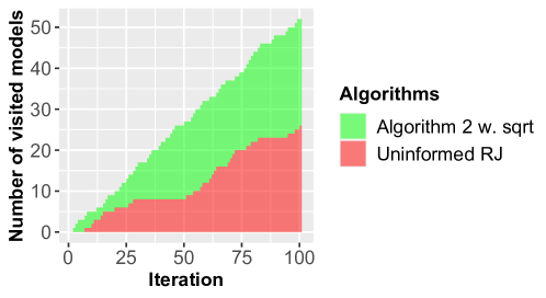
The performance of the different algorithms are summarized in Table 1 and Figure 2. The results for the uninformed RJ are based on 1,000 runs of 100,000 iterations, with burn-ins of 10,000. The uninformed RJ is in fact a “non-fully” informed RJ corresponding to Algorithm 2 with the only difference that $g(k,\cdot\,)=\mathcal{U}\{\mathbf{N}(k)\}$ instead of locally- or globally-balanced proposal distributions such that $g(k,k^{\prime})\propto h\left(\hat{\pi}(k^{\prime}\mid\mathbf{D}_{n})\big{/}\hat{\pi}(k\mid\mathbf{D}_{n})\right)$ for all $k^{\prime}\in\mathbf{N}(k)$. It may thus be seen as corresponding to the approach of Green (2003). For a fair comparison with this RJ, the number of iterations for which the fully informed RJ, i.e. Algorithm 2, is run is reduced to account for the additional complexity of using informed distributions $g(k,\cdot\,)$. The number of iterations has to be reduced to 85,000 to reach the same runtime as the uninformed RJ; one run takes about one minute in R on a i9 computer. To measure performance, we display the model-switching acceptance rates, model-visit rates and relative increases in TV with respect to the best sampler, which is Algorithm 2 with $h(x)=\sqrt{x}$. The TVs are in between approximated model distributions from RJ outputs and the posterior model PMF.

The model-switching acceptance rates are the acceptance rates, but computed considering only the iterations in which model switches are proposed. The visit rates are the average number of model switches in one run, reported per iteration. For both these measures, we count the number of accepted model switches, and this number is divided by either the number of proposed model switches or total number of iterations. These rates are thus similar but they convey different information: model-switching acceptance rates reflect the quality of the proposal distributions used during model switches, while visit rates measure the propensity to propose a switch to another model (and accept it). They together allow to understand why, for instance, Algorithm 2 with $h(x)=\sqrt{x}$ is (slightly) better than Algorithm 2 with $h(x)=x/(1+x)$ in terms of TV. Indeed, even if it has a (slightly) worse model-switch proposal scheme (model-switching acceptance rates: 66% vs 67%), it proposes more often to switch models (visit rates: 55% vs 53%), which has an impact on the TV.

Table 1: Performance of the uninformed and informed RJ in terms of model-switching acceptance rate, model-visit rate and relative increase in TV with respect to Algorithm 2 with $h(x)=\sqrt{x}$

Algorithms	Acc. rate	Visit rate	Rel. increase in TV
Algorithm 2 w. $h(x)=\sqrt{x}$	66%	55%	—
Algorithm 2 w. $h(x)=x/(1+x)$	67%	53%	2%
Uninformed RJ	30%	27%	28%
Algorithm 2 w. $h(x)=x$	57%	46%	40%

This robust-variable-selection application shows that even in a moderate-size example, in this case with 8 covariates and 256 models, the locally-balanced proposal distributions lead to RJ that can outperform RJ proposing models uniformly at random, at fixed computational budget. In contrast, the globally-balanced proposal distribution does not yield an improvement that is significant enough to compensate for the decrease in number of iterations. We observed that even when the RJ with the function $h(x)=x$ is run for the same number of iterations as the uniformed one, the former only slightly outperforms the latter.

For the informed RJ to be effective, the approximations on which they rely have to be accurate. Recall that their accuracy depends on the sample size (at least in some scenarios regarding the approximations of $\pi(\,\cdot\mid k^{\prime},\mathbf{D}_{n})$ by $q_{k\mapsto k^{\prime}}$, as explained in Section 3.1). In this example, $n=97$. To understand if this is actually large for such a robust-linear-regression problem with 8 covariates, we can compare the model-switching acceptance rates of Algorithm 2 with those of the ideal RJ they approximate. Recall that ideal RJ set $g(k,k^{\prime})\propto h\left(\pi(k^{\prime}\mid\mathbf{D}_{n})\big{/}\pi(k\mid\mathbf{D}_{n})\right)$ and $q_{k\mapsto k^{\prime}}=\pi(\,\cdot\mid k^{\prime},\mathbf{D}_{n})$. It is possible to evaluate their model-switching acceptance rates because these correspond to the acceptance rates of MH samplers targeting the PMF $\pi(\,\cdot\mid\mathbf{D}_{n})$ using $g(k,k^{\prime})\propto h\left(\pi(k^{\prime}\mid\mathbf{D}_{n})\big{/}\pi(k\mid\mathbf{D}_{n})\right)$, computed considering only iterations in which $k^{\prime}\neq k$ is proposed. When $h(x)=x/(1+x)$, the acceptance rate of the MH sampler is 88%, which is sufficiently close to 1 to suggest that the asymptotic regime presented in Zanella (2020) where the size of the discrete space increases and the acceptance probabilities converge to 1 is nearly reached. To understand which approximations explain the gap between Algorithm 2 with $h(x)=x/(1+x)$ and a model-switching acceptance rate of 67% and its ideal counterpart with a rate of 88%, we can look at the model-switching acceptance rate of a RJ using methods to sample parameter proposals from a distribution closer to $\pi(\,\cdot\mid k^{\prime},\mathbf{D}_{n})$ and next at that of a RJ additionally using a method making $g(k,k^{\prime})$ closer to being proportional to $h\left(\pi(k^{\prime}\mid\mathbf{D}_{n})\big{/}\pi(k\mid\mathbf{D}_{n})\right)$ (recall the overview of the methods presented in Section 2.4). It is 84% for the first RJ (with $T=N=10$), and it increases to 87% for the second RJ. Using such methods simply make RJ too computationally expensive to be competitive in this example. Recall that their precision parameters can be increased to make the second RJ arbitrarily close to the ideal one with a model-switching acceptance rate of 88%.

These results suggest that $n$ is of moderate size, in the sense that the approximations used in Algorithm 2 are good enough to yield an improvement, but it is expected that the improvement would be even more marked if we had access to more data points. Also, the results suggest that the approximations explaining the most part of the gap between Algorithm 2 with $h(x)=x/(1+x)$ and a model-switching acceptance rate of 67% and its ideal counterpart with a rate of 88% are the approximations of $\pi(\,\cdot\mid k^{\prime},\mathbf{D}_{n})$ by $q_{k\mapsto k^{\prime}}$. We investigated to see if there are significant differences between the covariance matrices used in $q_{k\mapsto k^{\prime}}$ and those of $\pi(\,\cdot\mid k^{\prime},\mathbf{D}_{n})$, and it is not the case. This means that the approximations of $\pi(\,\cdot\mid k^{\prime},\mathbf{D}_{n})$ by $q_{k\mapsto k^{\prime}}$ are not as accurate as we would like because the densities $\pi(\,\cdot\mid k^{\prime},\mathbf{D}_{n})$ are significantly different from bell curves. Our analysis also allows to rule out an issue with using the same observed covariance matrix as the normal regression in the robust LPTN framework. In fact, a robust-linear-regression analysis reveals the presence of outliers, but only for models with negligible posterior mass (both in the robust and non-robust frameworks). We finally note that, for models with non-negligible posterior mass, there is no gross violation of the assumptions underlying linear regression.

Figure 2: Number of visited models as a function of the iteration number in a typical run of the uninformed RJ and Algorithm 2 with $h(x)=\sqrt{x}$

5 Discussion

In this paper, we proposed simple fully-informed RJ and described the situations in which they are expected to be efficient: when the sample size is sufficiently large, Assumptions 1–2 of Section 3.1 are verified, some models among those considered well approximate the true data generating process and Bernstein-von Mises theorems hold for these models. Informed proposal distributions are crucial when the model probabilities and parameter densities vary significantly within neighbourhoods of states of the Markov chains. They are expected to vary significantly in the large-sample regime in which the target concentrates. But we noticed with our numerical example that they may vary greatly even when this large-sample regime is not reached. The proposed RJ show major improvements in this example as the chains spend less iterations at the same state, compared with the RJ that naively proposes models uniformly at random and thus often tries to reach low probability models, leading to higher rejection rates.

Yet, the proposed samplers are reversible which allows them to return to recently visited models often. The next step in the line of research of trans-dimensional samplers for non-nested model selection is to propose sampling schemes which do not suffer from this diffusive behaviour, but instead induce persistent movement in the model-indicator process. A first step in this direction has recently been made by Gagnon and Maire (2020), but their approach cannot be used in all contexts of non-nested model selection. It can nevertheless be applied in any variable-selection problem. It is however expected to be efficient when the posterior model mass is diffused over a large number of models with different number of covariates, which is not the case in our numerical example.

Appendix A Improving the approximations

In practice, the sample size may not be large enough for the approximations in the proposal mechanisms to be accurate. In Sections A.1 and A.2, we present the details of the methods reviewed in Section 2.4 that allow to improve upon the normal-distribution approximations to $\pi(\,\cdot\mid k,\mathbf{D}_{n})$. These methods turn out to be useful for improving upon the approximations forming the model proposal distributions $g(k,\cdot\,)$ as well; this is explained in detail in Section A.3.

A.1 RJ with the method of Karagiannis and Andrieu (2013)

In the definition of the annealing intermediate distributions $\rho_{k\mapsto k^{\prime}}^{(t)}$ in (8), it is considered that $\mathcal{D}_{k\mapsto k^{\prime}}(\mathbf{x}_{k},\mathbf{u}_{k\mapsto k^{\prime}})=(\mathbf{u}_{k\mapsto k^{\prime}},\mathbf{x}_{k})=(\mathbf{y}_{k^{\prime}},\mathbf{u}_{k^{\prime}\mapsto k})$, implying that $|J_{\mathcal{D}_{k\mapsto k^{\prime}}}(\mathbf{x}_{k},\mathbf{u}_{k\mapsto k^{\prime}})|=1$, and $q_{k^{\prime}\mapsto k}=\varphi(\,\cdot\,;\hat{\mathbf{x}}_{k},\hat{\mathcal{I}}_{k}^{-1})$. For the general definition, see Karagiannis and Andrieu (2013).

We now present in Algorithm 3 an informed RJ incorporating the method of Karagiannis and Andrieu (2013). Recall that the acceptance probability in this RJ is defined in (10). Note that Algorithm 3 corresponds to Algorithm 2 when $T=1$; no path is sampled in Step 2.(b).

Algorithm 3 RJ incorporating the method of Karagiannis and Andrieu (2013)

1. Sample $k^{\prime}\sim g(k,\cdot\,)$ with $g(k,k^{\prime})\propto h\left(\hat{\pi}(k^{\prime}\mid\mathbf{D}_{n})\big{/}\hat{\pi}(k\mid\mathbf{D}_{n})\right)$ for all $k^{\prime}\in\mathbf{N}(k)$.

2. If $k^{\prime}=k$, attempt a parameter update using a MCMC kernel of invariant distribution $\pi(\,\cdot\mid k,\mathbf{D}_{n})$ while keeping the value of the model indicator k fixed.

3. If $k^{\prime}\neq k$, sample $\mathbf{y}_{k^{\prime}}^{(0)}\sim\varphi(\,\cdot\,;\hat{\mathbf{x}}_{k^{\prime}},\hat{\mathcal{I}}_{k^{\prime}}^{-1})$ and $u\sim\mathcal{U}[0,1]$, and set $\mathbf{x}_{k}^{(0)}:=\mathbf{x}_{k}$. Sample a path $(\mathbf{x}_{k}^{(1)},\mathbf{y}_{k^{\prime}}^{(1)}),\ldots,(\mathbf{x}_{k}^{(T-1)},\mathbf{y}_{k^{\prime}}^{(T-1)})$, where $(\mathbf{x}_{k}^{(t)},\mathbf{y}_{k^{\prime}}^{(t)})\sim K_{k\mapsto k^{\prime}}^{(t)}((\mathbf{x}_{k}^{(t-1)},\mathbf{y}_{k^{\prime}}^{(t-1)}),\cdot\,)$. If $u\leq\alpha_{\text{RJ2}}((k,\mathbf{x}_{k}^{(0)}),(k^{\prime},\mathbf{y}_{k^{\prime}}^{(T-1)}))$ set the next state of the chain to $(k^{\prime},\mathbf{y}_{k^{\prime}}^{(T-1)})$. Otherwise, set it to $(k,\mathbf{x}_{k})$.

4. Go to Step 1.

Using the same proof technique as in Gagnon and Doucet (2021), it can be proved that under regularity conditions a Markov chain simulated by Algorithm 3 converges weakly to that of a RJ which is able to sample from $\pi(\,\cdot\,\mid k,\mathbf{D}_{n})$ for all $k$ with acceptance probabilities $\alpha_{\text{MH}}$ but using $g(k,k^{\prime})\propto h\left(\hat{\pi}(k^{\prime}\mid\mathbf{D}_{n})\big{/}\hat{\pi}(k\mid\mathbf{D}_{n})\right)$, as $T\longrightarrow\infty$, for fixed $n$. Note that the weak convergence in this case is not in probability because the target is considered non-random (contrarily to the framework under which Theorem 1 is stated).

As $T$ increases, it is expected that the acceptance probabilities increase steadily towards $\alpha_{\text{MH}}$ until convergence is reached. A RJ user thus has to find a balance between a RJ close to be ideal and the computational cost associated to this. As explained in Karagiannis and Andrieu (2013), the computational cost scales linearly with $T$. In some situations, the improvement as a function of $T$ is very marked for $T\leq T_{0}$, effectively offsetting the computational cost. This is not the case in our numerical example.

Karagiannis and Andrieu (2013) prove that under two conditions Algorithm 3 is valid, in the sense that the target distribution is an invariant distribution. These conditions are the following.

Symmetry condition:

For $t=1,\ldots,T-1$ the pairs of transition kernels $K_{k\mapsto k^{\prime}}^{(t)}(\,\cdot\,,\cdot\,)$ and $K_{k^{\prime}\mapsto k}^{(T-t)}(\,\cdot\,,\cdot\,)$ satisfy

$$K_{k\mapsto k^{\prime}}^{(t)}((\mathbf{x}_{k},\mathbf{y}_{k^{\prime}}),\cdot\,)=K_{k^{\prime}\mapsto k}^{(T-t)}((\mathbf{x}_{k},\mathbf{y}_{k^{\prime}}),\cdot\,)\quad\text{for any }(\mathbf{x}_{k},\mathbf{y}_{k^{\prime}}).$$ (13)

Reversibility condition:

For $t=1,\ldots,T-1$, and for any $(\mathbf{x}_{k},\mathbf{y}_{k^{\prime}})$ and $(\mathbf{x}_{k}^{\prime},\mathbf{y}_{k^{\prime}}^{\prime})$,

$$\rho_{k\mapsto k^{\prime}}^{(t)}(\mathbf{x}_{k},\mathbf{y}_{k^{\prime}})\,K_{k\mapsto k^{\prime}}^{(t)}((\mathbf{x}_{k},\mathbf{y}_{k^{\prime}}),(\mathbf{x}_{k}^{\prime},\mathbf{y}_{k^{\prime}}^{\prime}))=\rho_{k\mapsto k^{\prime}}^{(t)}(\mathbf{x}_{k}^{\prime},\mathbf{y}_{k^{\prime}}^{\prime})\,K_{k\mapsto k^{\prime}}^{(t)}((\mathbf{x}_{k}^{\prime},\mathbf{y}_{k^{\prime}}^{\prime}),(\mathbf{x}_{k},\mathbf{y}_{k^{\prime}})).$$ (14)

As mentioned in Karagiannis and Andrieu (2013), (13) is verified if for all $t$, $K_{k\mapsto k^{\prime}}^{(t)}(\,\cdot\,,\cdot\,)$ and $K_{k^{\prime}\mapsto k}^{(T-t)}(\,\cdot\,,\cdot\,)$ are MH kernels sharing the same proposal distributions. (14) is satisfied if $K_{k\mapsto k^{\prime}}^{(t)}(\,\cdot\,,\cdot\,)$ is a MH kernel targeting $\rho_{k\mapsto k^{\prime}}^{(t)}$. We recommend to use MALA (Metropolis-adjusted Langevin algorithm, Roberts and Tweedie (1996)) proposal distributions whenever this is possible; see Karagiannis and Andrieu (2013) for other examples. If MALA proposal distributions are used, a step size is required for each pair $(k,k^{\prime})$ defining a transition from Model $k$ to Model $k^{\prime}$. For any of these model switches, we recommend to set the step size to $\ell/(d_{k}+d_{k^{\prime}})^{1/6}$, according to the findings in Roberts and Rosenthal (1998), and to tune $\ell$. To achieve the latter, do a line search with a fixed value of $T$ and choose $\ell$ that maximizes the model-switching acceptance rate, so that the resulting RJ is the closest to the ideal one.

A.2 RJ with additionally the method of Andrieu et al. (2018)

Denote the $N$ estimates of $\pi(k^{\prime}\mid\mathbf{D}_{n})/\pi(k\mid\mathbf{D}_{n})$ produced by the scheme of Karagiannis and Andrieu (2013) by $r_{\text{RJ2}}((k,\mathbf{x}_{k}^{(0)}),(k^{\prime},\mathbf{y}_{k^{\prime}}^{(T-1,1)})),\ldots,r_{\text{RJ2}}((k$, $\mathbf{x}_{k}^{(0)}),(k^{\prime},\mathbf{y}_{k^{\prime}}^{(T-1,N)}))$. Denote the average (with simplified notation) by

$$\bar{r}(k,k^{\prime}):=\frac{1}{N}\sum_{j=1}^{N}r_{\text{RJ2}}((k,\mathbf{x}_{k}^{(0)}),(k^{\prime},\mathbf{y}_{k^{\prime}}^{(T-1,j)})).$$

We now present in Algorithm 4 the RJ additionally incorporating the method of Andrieu et al. (2018).

Algorithm 4 RJ additionally incorporating the method of Andrieu et al. (2018)

1. Sample $k^{\prime}\sim g(k,\cdot\,)$ with $g(k,k^{\prime})\propto h\left(\hat{\pi}(k^{\prime}\mid\mathbf{D}_{n})\big{/}\hat{\pi}(k\mid\mathbf{D}_{n})\right)$ for all $k^{\prime}\in\mathbf{N}(k)$.

2. If $k^{\prime}=k$, attempt a parameter update using a MCMC kernel of invariant distribution $\pi(\,\cdot\mid k,\mathbf{D}_{n})$ while keeping the value of the model indicator k fixed.

3. If $k^{\prime}\neq k$, generate $u_{a},u_{c}\sim\mathcal{U}(0,1)$. If $u_{c}\leq 1/2$ go to Step 2.(b-i), otherwise go to Step 2.(b-ii).

4. Sample $N$ proposals $\mathbf{y}_{k^{\prime}}^{(T-1,1)},\ldots,\mathbf{y}_{k^{\prime}}^{(T-1,N)}$ as in Step 2.(b) of Algorithm 3. Sample $j^{*}$ from a PMF such that $\mathbb{P}(J^{*}=j)\propto r_{\text{RJ2}}((k,\mathbf{x}_{k}),(k^{\prime},\mathbf{y}_{k^{\prime}}^{(T-1,j)}))$. If

   $$u_{a} \leq\frac{g(k^{\prime},k)}{g(k,k^{\prime})}\,\bar{r}(k,k^{\prime}),$$

   set the next state of the chain to $(k^{\prime},\mathbf{y}_{k^{\prime}}^{(T-1,j^{*})})$. Otherwise, set it to $(k,\mathbf{x}_{k})$.

5. Sample one forward path as in Step 2.(b) of Algorithm 3. Denote the endpoint by $\mathbf{y}_{k^{\prime}}^{(T-1,1)}$. From $\mathbf{y}_{k^{\prime}}^{(T-1,1)}$, sample $N-1$ reverse paths again as in Step 2.(b) of Algorithm 3, yielding $N-1$ proposals for the parameters of Model $k$. If

   $$u_{a} \leq\frac{g(k^{\prime},k)}{g(k,k^{\prime})}\,\bar{r}(k^{\prime},k)^{-1},$$

   set the next state of the chain to $(k^{\prime},\mathbf{y}_{k^{\prime}}^{(T-1,1)})$. Otherwise, set it to $(k,\mathbf{x}_{k})$.

6. Go to Step 1.

No additional assumptions to those presented in Section A.1 are required to guarantee that Algorithm 4 is valid. Andrieu et al. (2018) prove that increasing $N$ decreases monotonically the asymptotic variances of the Monte Carlo estimates produced by RJ incorporating their approach.

It is expected that increasing $N$ (as increasing $T$ in the last section) leads to a steady increase in the acceptance probabilities until convergence is reached. As with Algorithm 3, there exists a balance between a RJ close to be ideal and the computational cost associated to this. An advantage of the approach presented in this section is that several operations can be executed in parallel, so that the computational burden is alleviated. The computational cost (over that of using the approach of Karagiannis and Andrieu (2013)) nevertheless depends on $N$ because computational overheads have to be taken into account. In our numerical example, the improvement as a function of $N$ is not significant enough to offset the computational cost.

A.3 Improving the model proposal distribution

We have seen in Section A.2 that $\bar{r}(k,k^{\prime})$ and the ratios $r_{\text{RJ2}}$ forming it are estimators of $\pi(k^{\prime}\mid\mathbf{D}_{n})/\pi(k\mid\mathbf{D}_{n})$. They can thus be used to enhance the approximations to the posterior probability ratios in $g(k,\cdot\,)$.

If we want to enhance the PMF $g(k,\cdot\,)$, we need to improve $\widehat{\pi}(l\mid\mathbf{D}_{n})/\widehat{\pi}(k\mid\mathbf{D}_{n})$ for all $l\in\mathbf{N}(k)$ as these are all involved in the construction of the PMF. Also, once $k^{\prime}$ has been sampled, we need to do the same for $g(k^{\prime},\cdot\,)$ given that this PMF comes into play in the computation of the acceptance probabilities (see, e.g., Algorithm 4). We thus need parameter proposals $\mathbf{y}_{l}^{(T-1,1)},\ldots,\mathbf{y}_{l}^{(T-1,N)}$ for all Models $l\in\mathbf{N}(k)$, and also for all models belonging to $\mathbf{N}(k^{\prime})$. The ratios $r_{\text{RJ2}}$ are next computed.

There are several ways to combine these ratios with $\widehat{\pi}(l\mid\mathbf{D}_{n})/\widehat{\pi}(k\mid\mathbf{D}_{n})$ and $\widehat{\pi}(s\mid\mathbf{D}_{n})/\widehat{\pi}(k^{\prime}\mid\mathbf{D}_{n})$ to improve the estimation of $\pi(l\mid\mathbf{D}_{n})/\pi(k\mid\mathbf{D}_{n})$ and $\pi(s\mid\mathbf{D}_{n})/\pi(k^{\prime}\mid\mathbf{D}_{n})$. We define the improved version of the PMF $g$ as follows to reflect this flexibility:

$$g_{\text{imp.}}(k,k^{\prime},\mathbf{x}_{k\mapsto\bullet}^{(0:T-1,\bullet)},\mathbf{y}_{\bullet}^{(0:T-1,\bullet)}):=h\left(\frac{\tilde{\pi}(k^{\prime}\mid\mathbf{D}_{n})}{\tilde{\pi}(k\mid\mathbf{D}_{n})}\right)\bigg{/}c_{\text{imp.}}(k),$$ (15)

where

$$\frac{\tilde{\pi}(k^{\prime}\mid\mathbf{D}_{n})}{\tilde{\pi}(k\mid\mathbf{D}_{n})} :=\varrho\left(\frac{\widehat{\pi}(k^{\prime}\mid\mathbf{D}_{n})}{\widehat{\pi}(k\mid\mathbf{D}_{n})},r_{\text{RJ2}}((k,\mathbf{x}_{k}^{(0)}),(k^{\prime},\mathbf{y}_{k^{\prime}}^{(T-1,1)})),\ldots,r_{\text{RJ2}}((k,\mathbf{x}_{k}^{(0)}),(k^{\prime},\mathbf{y}_{k^{\prime}}^{(T-1,N)}))\right),$$

$\mathbf{y}_{\bullet}^{(0:T-1,\bullet)}$ is the vector containing $\mathbf{y}_{l}^{(0,j)},\ldots,\mathbf{y}_{l}^{(T-1,j)}$ for all $j\in\{1,\ldots,N\}$ and $l\in\mathbf{N}(k)$, and $c_{k}^{\text{imp.}}$ is the normalizing constant. $\varrho$ is a function aiming at putting together the information; its choice is discussed below. $\mathbf{x}_{k\mapsto\bullet}^{(0:T-1,\bullet)}$ is the vector containing $\mathbf{x}_{k\mapsto l}^{(0,j)},\ldots,\mathbf{x}_{k\mapsto l}^{(T-1,j)}$ for all $j\in\{1,\ldots,N\}$ and $l\in\mathbf{N}(k)$. Here we added the subscript $k\mapsto l$ and superscript $(t,j)$ to highlight that the sequence generated using Step 2.(b) of Algorithm 3 depends on $j$ (different sequences are generated for different $j$), and also on $l$ through $\rho_{k\mapsto l}^{(t)}$ (8). Note that $\tilde{\pi}(l\mid\mathbf{D}_{n})/\tilde{\pi}(k\mid\mathbf{D}_{n})$ is an estimator of $\pi(l\mid\mathbf{D}_{n})/\pi(k\mid\mathbf{D}_{n})$ which is in fact a function of $\mathbf{x}_{k\mapsto l}^{(0,j)},\ldots,\mathbf{x}_{k\mapsto l}^{(T-1,j)}$ and $\mathbf{y}_{l}^{(0,j)},\ldots,\mathbf{y}_{l}^{(T-1,j)}$ for all $j\in\{1,\ldots,N\}$ additionally to $k$ and $l$; we used this notation to simplify and make the connection with $\widehat{\pi}(l\mid\mathbf{D}_{n})/\widehat{\pi}(k\mid\mathbf{D}_{n})$.

Algorithm 5 includes the idea of improving $\widehat{\pi}(l\mid\mathbf{D}_{n})/\widehat{\pi}(k\mid\mathbf{D}_{n})$ using ratios $r_{\text{RJ2}}$ in a valid way (as indicated by Proposition 2 below). This algorithm is quite complicated, but once a code for Algorithm 4 has been written, we can use the connections between Algorithm 5 and Algorithm 4 to facilitate the coding of the former. Another drawback of Algorithm 5 is that it requires to perform the computations for $g_{\text{imp.}}(k^{\prime},\cdot\,)$ even when $k^{\prime}=k$. This is because $g_{\text{imp.}}(k,k^{\prime},\mathbf{x}_{k\mapsto\bullet}^{(0:T-1,\bullet)},\mathbf{y}_{\bullet}^{(0:T-1,\bullet)})$ is different from $g_{\text{imp.}}(k^{\prime},k,\mathbf{y}_{k^{\prime}\mapsto\bullet}^{(0:T-1,j^{*})}$, $\mathbf{z}_{\bullet}^{(0:T-1,j^{*})},\mathbf{z}_{\bullet}^{(0:T-1,\bullet)})$ (see Step 2.(i)), even when $k^{\prime}=k$. At least, most of computations for the two main steps (Steps 2.(i) and 2.(ii)) can be performed in parallel. Again, computational overheads have to be taken into account. In our numerical example, the improvement is not significant enough to offset the computational cost.

Algorithm 5 RJ additionally improving the model proposal distribution

1. Sample $u_{a},u_{c}\sim\mathcal{U}(0,1)$. If $u_{c}\leq 1/2$ go to Step 2.(i), otherwise go to Step 2.(ii).

2. Do:

   1. For all $l\in\mathbf{N}(k)$, sample proposals as in Step 2.(b-i) of Algorithm 4: from $\mathbf{x}_{k}$, sample $N$ proposals $\mathbf{y}_{l}^{(T-1,1)},\ldots,\mathbf{y}_{l}^{(T-1,N)}$ as in Step 2.(b) of Algorithm 3.

   2. Compute $\tilde{\pi}(l\mid\mathbf{D}_{n})\big{/}\tilde{\pi}(k\mid\mathbf{D}_{n})$ for all $l\in\mathbf{N}(k)$ and $g_{\text{imp.}}(k,\cdot\,)$ as in (15).

   3. Sample $k^{\prime}\sim g_{\text{imp.}}(k,\cdot\,)$ and $j^{*}$ from a PMF such that $\mathbb{P}(J^{*}=j)\propto r_{\text{RJ2}}((k,\mathbf{x}_{k}^{(0)}),(k^{\prime},\mathbf{y}_{k^{\prime}}^{(T-1,j)}))$, and compute $\bar{r}(k,k^{\prime})$.

   4. For all $s\in\mathbf{N}(k^{\prime})\setminus\{k\}$, sample proposals as in Step 2.(b-ii) of Algorithm 4: from $\mathbf{y}_{k^{\prime}}^{(T-1,j^{*})}$, sample one path as in Step 2.(b) of Algorithm 3. Denote the endpoint by $\mathbf{z}_{s}^{(0,j^{*})}$. From $\mathbf{z}_{s}^{(0,j^{*})}$, sample $N-1$ reverse paths again as in Step 2.(b) of Algorithm 3, yielding $N-1$ proposals for the parameters of Model $k^{\prime}$ that we denote by $\mathbf{z}_{s\mapsto k^{\prime}}^{(T-1,j)}$, $j\in\{1,\ldots,N\}\setminus\{j^{*}\}$.

   5. Compute $\tilde{\pi}(s\mid\mathbf{D}_{n})\big{/}\tilde{\pi}(k^{\prime}\mid\mathbf{D}_{n})$ for all $s\in\mathbf{N}(k^{\prime})\setminus\{k\}$. Compute $g_{\text{imp.}}(k^{\prime},\cdot\,)$ using these and $(\tilde{\pi}(k^{\prime}\mid\mathbf{D}_{n})\big{/}\tilde{\pi}(k\mid\mathbf{D}_{n}))^{-1}$ computed in (b).

   6. If

      $$u_{a} \leq\frac{g_{\text{imp.}}(k^{\prime},k,\mathbf{y}_{k^{\prime}\mapsto\bullet}^{(0:T-1,j^{*})},\mathbf{z}_{\bullet}^{(0:T-1,j^{*})},\mathbf{z}_{\bullet}^{(0:T-1,\bullet)})}{g_{\text{imp.}}(k,k^{\prime},\mathbf{x}_{k\mapsto\bullet}^{(0:T-1,\bullet)},\mathbf{y}_{\bullet}^{(0:T-1,\bullet)})}\,\bar{r}(k,k^{\prime}),$$

      set the next state of the chain to $(k^{\prime},\mathbf{y}_{k^{\prime}}^{(T-1,j^{*})})$. Otherwise, set it to $(k,\mathbf{x}_{k})$.

3. Do:

   1. For all $l\in\mathbf{N}(k)$, sample proposals as in Step 2.(b-ii) of Algorithm 4: from $\mathbf{x}_{k}$, sample one path as in Step 2.(b) of Algorithm 3. Denote the endpoint by $\mathbf{y}_{l}^{(T-1,1)}$. From $\mathbf{y}_{l}^{(T-1,1)}$, sample $N-1$ reverse paths again as in Step 2.(b) of Algorithm 3, yielding $N-1$ proposals for the parameters of Model $k$ that we denote by $\mathbf{y}_{l\mapsto k}^{(0,2)},\ldots,\mathbf{y}_{l\mapsto k}^{(0,N)}$.

   2. Compute $\tilde{\pi}(l\mid\mathbf{D}_{n})\big{/}\tilde{\pi}(k\mid\mathbf{D}_{n})$ for all $l\in\mathbf{N}(k)$ and $g_{\text{imp.}}(k,\cdot\,)$ as in (15).

   3. Sample $k^{\prime}\sim g_{\text{imp.}}(k,\cdot\,)$ and compute $\bar{r}(k^{\prime},k)^{-1}$.

   4. For all $s\in\mathbf{N}(k^{\prime})\setminus\{k\}$, sample proposals as in Step 2.(b-i) of Algorithm 4: from $\mathbf{y}_{k^{\prime}}^{(T-1,1)}$, sample $N$ proposals $\mathbf{z}_{s}^{(0,1)},\ldots,\mathbf{z}_{s}^{(0,N)}$ as in Step 2.(b) of Algorithm 3.

   5. Compute $\tilde{\pi}(s\mid\mathbf{D}_{n})\big{/}\tilde{\pi}(k^{\prime}\mid\mathbf{D}_{n})$ for all $s\in\mathbf{N}(k^{\prime})\setminus\{k\}$. Compute $g_{\text{imp.}}(k^{\prime},\cdot\,)$ using these and $(\tilde{\pi}(k^{\prime}\mid\mathbf{D}_{n})\big{/}\tilde{\pi}(k\mid\mathbf{D}_{n}))^{-1}$ computed in (b).

   6. If

      $$u_{a} \leq\frac{g_{\text{imp.}}(k^{\prime},k,\mathbf{y}_{k^{\prime}\mapsto\bullet}^{(0:T-1,1)},\mathbf{z}_{\bullet}^{(0:T-1,\bullet)})}{g_{\text{imp.}}(k,k^{\prime},\mathbf{x}_{k\mapsto\bullet}^{(0:T-1,1)},\mathbf{y}_{\bullet}^{(0:T-1,1)},\mathbf{y}_{\bullet\mapsto k}^{(0:T-1,\bullet)})}\,\bar{r}(k^{\prime},k)^{-1},$$

      set the next state of the chain to $(k^{\prime},\mathbf{y}_{k^{\prime}}^{(T-1,1)})$. Otherwise, set it to $(k,\mathbf{x}_{k})$.

4. Go to Step 1.

Proposition 2.

Under the two assumptions presented in Section A.1, (13)–(14), Algorithm 5 is valid.

It is natural to set $\tilde{\pi}(l\mid\mathbf{D}_{n})/\tilde{\pi}(k\mid\mathbf{D}_{n})$ to 1 when $l=k$. This implies that we in fact do not need to sample proposals for Model $k$ in the first parts of Steps 2.(i) and 2.(ii). Also, in the second parts of Steps 2.(i) and 2.(ii), it is not required to sample proposals for $s=k^{\prime}$ for the same reason. When $k^{\prime}=k$, we actually perform a “vanilla” parameter-update step (an HMC step in our numerical example). In this case, the MH ratio as to be multiplied by

$$\frac{g_{\text{imp.}}(k^{\prime},k,\mathbf{y}_{k^{\prime}\mapsto\bullet}^{(0:T-1,j^{*})},\mathbf{z}_{\bullet}^{(0:T-1,j^{*})},\mathbf{z}_{\bullet}^{(0:T-1,\bullet)})}{g_{\text{imp.}}(k,k^{\prime},\mathbf{x}_{k\mapsto\bullet}^{(0:T-1,\bullet)},\mathbf{y}_{\bullet}^{(0:T-1,\bullet)})}$$

or

$$\frac{g_{\text{imp.}}(k^{\prime},k,\mathbf{y}_{k^{\prime}\mapsto\bullet}^{(0:T-1,1)},\mathbf{z}_{\bullet}^{(0:T-1,\bullet)})}{g_{\text{imp.}}(k,k^{\prime},\mathbf{x}_{k\mapsto\bullet}^{(0:T-1,1)},\mathbf{y}_{\bullet}^{(0:T-1,1)},\mathbf{y}_{\bullet\mapsto k}^{(0:T-1,\bullet)})},$$

depending if Step 2.(i) or Step 2.(ii) is used.

The function $\varrho$ in (15) specifies the way the information is combined. It may be set for instance to the simple average:

$$\frac{\tilde{\pi}(l\mid\mathbf{D}_{n})}{\tilde{\pi}(k\mid\mathbf{D}_{n})}=\frac{1}{N+1}\left(\frac{\widehat{\pi}(l\mid\mathbf{D}_{n})}{\widehat{\pi}(k\mid\mathbf{D}_{n})}+\sum_{j=1}^{N}r_{\text{RJ2}}((k,\mathbf{x}_{k}^{(0)}),(l,\mathbf{y}_{l}^{(T-1,j)}))\right).$$ (16)

One may alternatively take the average of $\widehat{\pi}(l\mid\mathbf{D}_{n})/\widehat{\pi}(k\mid\mathbf{D}_{n})$ and $\bar{r}(k,l)$:

$$\frac{\tilde{\pi}(l\mid\mathbf{D}_{n})}{\tilde{\pi}(k\mid\mathbf{D}_{n})} =\frac{1}{2}\left(\frac{\widehat{\pi}(l\mid\mathbf{D}_{n})}{\widehat{\pi}(k\mid\mathbf{D}_{n})}+\bar{r}(k,l)\right)$$

$$=\frac{1}{2}\left(\frac{\widehat{\pi}(l\mid\mathbf{D}_{n})}{\widehat{\pi}(k\mid\mathbf{D}_{n})}+\frac{1}{N}\sum_{j=1}^{N}r_{\text{RJ2}}((k,\mathbf{x}_{k}^{(0)}),(l,\mathbf{y}_{l}^{(T-1,j)}))\right).$$

These reflect a choice of putting more or less weight on $\widehat{\pi}(l\mid\mathbf{D}_{n})/\widehat{\pi}(k\mid\mathbf{D}_{n})$. We know that if $T$ and $N$ are large enough then $\bar{r}(k,l)$ is close to $\pi(l\mid\mathbf{D}_{n})/\pi(k\mid\mathbf{D}_{n})$, which may not be the case for $\widehat{\pi}(l\mid\mathbf{D}_{n})/\widehat{\pi}(k\mid\mathbf{D}_{n})$ when $n$ is not sufficiently large. The latter ratio may thus act as outlying/conflicting information against which these averages above are not robust. A robust approach consists in setting $\varrho$ to be the median of $\widehat{\pi}(l\mid\mathbf{D}_{n})/\widehat{\pi}(k\mid\mathbf{D}_{n}),r_{\text{RJ2}}((k,\mathbf{x}_{k}^{(0)}),(l,\mathbf{y}_{l}^{(T-1,1)}))$, $\ldots,r_{\text{RJ2}}((k,\mathbf{x}_{k}^{(0)}),(l,\mathbf{y}_{l}^{(T-1,N)}))$. We recommend this approach and use it in our numerical example.

Furthermore, as $T,N\longrightarrow\infty$, $\tilde{\pi}(l\mid\mathbf{D}_{n})/\tilde{\pi}(k\mid\mathbf{D}_{n})$ is a consistent estimator of $\pi(l\mid\mathbf{D}_{n})/\pi(k\mid\mathbf{D}_{n})$ for fixed $n$ when the median or (16) is used (recall the properties of $r_{\text{RJ2}}$ and $\bar{r}$ mentioned in Sections A.1 and A.2). Therefore, if the function $h$ is such that $h(x)=x\,h(1/x)$ for $x>0$, then the acceptance probabilities in Algorithm 5 converge towards $1\wedge c(k)/c(k^{\prime})$, where $c(k)$ and $c(k^{\prime})$ are the normalizing constants with

$$c(k)=\sum_{l\in\mathbf{N}(k)}h\left(\frac{\pi(l\mid\mathbf{D}_{n})}{\pi(k\mid\mathbf{D}_{n})}\right).$$

In fact, the same technique as in the proof of Theorem 1 in Gagnon and Doucet (2021) allows to prove that a Markov chain simulated by Algorithm 5 converges weakly for fixed $n$ to that of an ideal RJ which has access to the unnormalized version of the posterior probabilities $\pi(k\mid\mathbf{D}_{n})$ and is able to sample from the conditional distributions $\pi(\,\cdot\mid k,\mathbf{D}_{n})$ (and for which the acceptance probabilities are $1\wedge c(k)/c(k^{\prime})$), with its good mixing properties as discussed in Section 1.3.

Appendix B Details of the variable-selection example

We review linear regression and introduce notation in Section B.1. We present in Section B.2 all the details to compute estimates for the normal linear-regression model. Some are useful for the computation of algorithm inputs, such as the observed information matrix, and to verify the validity of our RJ code (as mentioned in Section 4.1). In Section B.3, we turn to the details of the robust linear regressions and the computation of algorithm inputs.

B.1 Linear regression

We first introduce notation. We define $\gamma_{1},\ldots,\gamma_{n}\in\mathbb{R}$ to be $n$ data points from the dependent variable, and $\boldsymbol{\gamma}_{n}:=(\gamma_{1},\ldots,\gamma_{n})^{T}$. We denote the full design matrix containing $n$ observations from all covariates by $\mathbf{C}\in\mathbb{R}^{n\times p}$, where $p$ is a positive integer. For simplicity, we refer to the first column of $\mathbf{C}$ as the first covariate even if, as usual, it is a column of $1$’s. The design matrix associated with Model $k$ whose columns form a subset of $\mathbf{C}$ is denoted by $\mathbf{C}_{k}$, with lines denoted by $\mathbf{c}_{i,k}^{T}$. We use $d_{k}$ to denote the number of covariates in Model $k$; we therefore slightly abuse notation given that the number of parameters for Model $k$ is $d_{k}+1$ (one regression coefficient per covariate plus the scale parameter of the error term).

The linear regression is

$$\gamma_{i}=\mathbf{c}_{i,K}^{T}\,\boldsymbol{\beta}_{K}+\epsilon_{i,K},\quad i=1,\ldots,n,\quad K\in\mathcal{K},$$

where $K$ is the model indicator, $\boldsymbol{\beta}_{K}$ is the random vector containing the regression coefficients of Model $K$ and $\epsilon_{1,K},\ldots,\epsilon_{n,K}\in\mathbb{R}$ are the random errors of Model $K$. We assume that $\epsilon_{1,K},\ldots,\epsilon_{n,K}$ and $\boldsymbol{\beta}_{K}$ are $n+1$ conditionally independent random variables given $(K,\sigma_{K})$, with $\sigma_{K}>0$ being the scale parameter of the errors of Model $K$. The conditional density of $\epsilon_{i,K}$ is given by

$$\epsilon_{i,K}\mid K,\sigma_{K},\boldsymbol{\beta}_{K}\stackrel{{\scriptstyle d}}{{=}}\epsilon_{i,K}\mid K,\sigma_{K}\stackrel{{\scriptstyle d}}{{\sim}}(1/\sigma_{K})f(\epsilon_{i,K}/\sigma_{K}),\quad i=1,\ldots,n.$$

B.2 Normal linear regression

We present in this section a result giving the precise form of the joint posterior density for the normal linear regression.

Proposition 3.

If $f=\varphi(\,\cdot\,;0,1)$ and $\pi(\boldsymbol{\beta}_{k},\sigma_{k}\mid k)\propto 1/\sigma_{k}$, then

$$\pi(k\mid\boldsymbol{\gamma}_{n})\propto\pi(k)\,\frac{\Gamma((n-d_{k})/2)\,\pi^{d_{k}/2}}{\|\boldsymbol{\gamma}_{n}-\widehat{\boldsymbol{\gamma}}_{k}\|_{2}^{n-d_{k}}\,|\mathbf{C}_{k}^{T}\mathbf{C}_{k}|^{1/2}},$$ (17)

$$\pi(\sigma_{k}\mid k,\boldsymbol{\gamma}_{n})=\frac{2^{1-\frac{n-d_{k}}{2}}\|\boldsymbol{\gamma}_{n}-\widehat{\boldsymbol{\gamma}}_{k}\|_{2}^{n-d_{k}}}{\Gamma((n-d_{k})/2)\,\sigma_{k}^{n-d_{k}+1}}\,\exp\left\{-\frac{1}{2\sigma_{k}^{2}}\,\|\boldsymbol{\gamma}_{n}-\widehat{\boldsymbol{\gamma}}_{k}\|_{2}^{2}\right\},$$

and

$$\boldsymbol{\beta}_{K}\mid K,\sigma_{K},\boldsymbol{\gamma}_{n}\sim\varphi(\,\cdot\,;\widehat{\boldsymbol{\beta}}_{k},\sigma_{K}^{2}(\mathbf{C}_{K}^{T}\mathbf{C}_{K})^{-1}),$$

where $\widehat{\boldsymbol{\gamma}}_{k}:=\mathbf{C}_{k}(\mathbf{C}_{k}^{T}\mathbf{C}_{k})^{-1}\mathbf{C}_{k}^{T}\boldsymbol{\gamma}_{n}$, $\widehat{\boldsymbol{\beta}}_{k}:=(\mathbf{C}_{K}^{T}\mathbf{C}_{K})^{-1}\mathbf{C}_{K}^{T}\boldsymbol{\gamma}_{n}$, and $\|\cdot\|_{2}$ is the Euclidian norm. Note that the normalization constant of $\pi(k\mid\boldsymbol{\gamma}_{n})$ is the sum over $k$ of the expression on the right-hand side (RHS) in (17).

Note that $\sigma_{K}^{2}\mid K,\boldsymbol{\gamma}_{n}$ has an inverse-gamma distribution with shape and scale parameters given by $(n-d_{k})/2$ and $\|\boldsymbol{\gamma}_{n}-\widehat{\boldsymbol{\gamma}}_{k}\|_{2}^{2}/2$, respectively. We work on the log-scale for the scale parameters so that all the parameters take values on the real line, and presumably, have densities that are closer to the bell curve. We thus define $\eta_{k}:=\log\sigma_{k}$. The associated conditional distribution is given by

$$\pi(\eta_{k}\mid k,\boldsymbol{\gamma}_{n}):=\frac{2^{1-\frac{n-d_{k}}{2}}\|\boldsymbol{\gamma}_{n}-\widehat{\boldsymbol{\gamma}}_{k}\|_{2}^{n-d_{k}}}{\Gamma((n-d_{k})/2)\,\mathrm{e}^{(n-d_{k})\eta_{k}}}\,\exp\left\{-\frac{1}{2\mathrm{e}^{2\eta_{k}}}\,\|\boldsymbol{\gamma}_{n}-\widehat{\boldsymbol{\gamma}}_{k}\|_{2}^{2}\right\}.$$

The other terms in the joint posterior do not change except that we now consider that $\boldsymbol{\beta}_{K}\mid K,\eta_{K},\boldsymbol{\gamma}_{n}\sim\varphi(\,\cdot\,;\widehat{\boldsymbol{\beta}}_{k},\exp(2\eta_{K})(\mathbf{C}_{K}^{T}\mathbf{C}_{K})^{-1})$.

The maximizers of the conditional posterior densities given that $K=k$ are:

$$\hat{\mathbf{x}}_{k}=(\widehat{\boldsymbol{\beta}}_{k},\widehat{\eta}_{k}),$$

where

$$\widehat{\eta}_{k}:=\log\sqrt{\frac{1}{n}\,\|\boldsymbol{\gamma}_{n}-\widehat{\boldsymbol{\gamma}}_{k}\|_{2}^{2}}.$$

The observed information matrix evaluated at the maximizers is thus given by

$$\hat{\mathcal{I}}_{k}=\left(\begin{array}[]{cc}\mathbf{C}_{k}^{T}\mathbf{C}_{k}/\mathrm{e}^{2\hat{\eta}_{k}}&\mathbf{0}\cr\mathbf{0}&2n\end{array}\right).$$

Then,

$$\hat{\mathcal{I}}_{k}^{-1}=\left(\begin{array}[]{cc}\mathrm{e}^{2\hat{\eta}_{k}}(\mathbf{C}_{k}^{T}\mathbf{C}_{k})^{-1}&\mathbf{0}\cr\mathbf{0}&(2n)^{-1}\end{array}\right).$$ (20)

Relying on improper priors such as $\pi(\boldsymbol{\beta}_{k},\sigma_{k}\mid k)\propto 1/\sigma_{k}$ may lead to inconsistencies in model selection (see, e.g., Casella et al. (2009)). When this problem happens, the phenomenon is referred to as the Jeffreys-Lindley paradox (Lindley (1957) and Jeffreys (1967)) in the literature. It can be shown that the Jeffreys-Lindley paradox does not arise under the framework of normal linear regression described above when the prior distribution on $K$ is carefully chosen, and more precisely, set to

$$\pi(k)\propto|\mathbf{C}_{k}^{T}\mathbf{C}_{k}|^{1/2}/n^{d_{k}/2}.$$

See Gagnon et al. (2021) for an analogous proof in a framework of principal component regression.

When the covariates are orthonormal, $|\mathbf{C}_{k}^{T}\mathbf{C}_{k}|^{1/2}=|n\mathbf{I}_{d_{k}}|^{1/2}=n^{d_{k}/2}$ (if all covariate observations are standardized using a standard deviation in which the divisor is $n$). In this case, $\pi(k)\propto|\mathbf{C}_{k}^{T}\mathbf{C}_{k}|^{1/2}/n^{d_{k}/2}=1$. The proposed prior on $K$ can thus be seen as a relative adjustment of the volume spanned by the columns of $\mathbf{C}_{K}^{T}\mathbf{C}_{K}$.

B.3 Robust linear regression

In this section, we consider that the density $f$ is a LPTN with parameter $\rho\in(2\Phi(1)-1,1)\approx(0.6827,1)$, i.e.

$$f(x)=\left\{\begin{array}[]{lcc}\varphi(x;0,1)&\text{ if }&\left|x\right|\leq\tau,\\ \varphi(\tau;0,1)\,\frac{\tau}{|x|}\left(\frac{\log\tau}{\log|x|}\right)^{\lambda+1}&\text{ if }&\left|x\right|>\tau,\\ \end{array}\right.$$ (21)

where $x\in\mathbb{R}$ and $\Phi(\,\cdot\,)$ is the cumulative distribution function (CDF) of a standard normal. The terms $\tau>1$ and $\lambda>0$ are functions of $\rho$ and satisfy

$$\tau=\{\tau:\mathbb{P}(-\tau\leq Z\leq\tau)=\rho\,\text{ for }\,Z\sim\varphi(\,\cdot\,;0,1)\},$$

$$\lambda=2(1-\rho)^{-1}\varphi(\tau;0,1)\,\tau\log(\tau).$$

Setting $\rho$ to $0.95$ has proved to be suitable for practical purposes (see Gagnon et al. (2020a)). Accordingly, this is the value that is used in our numerical example.

Using the same prior as the normal regression, the joint posterior density is:

$$\pi(k,\boldsymbol{\beta}_{k},\sigma_{k}\mid\boldsymbol{\gamma}_{n})\propto\frac{|\mathbf{C}_{k}^{T}\mathbf{C}_{k}|^{1/2}}{n^{d_{k}/2}}\frac{1}{\sigma_{k}}\prod_{i=1}^{n}\frac{1}{\sigma_{k}}f\left(\frac{\gamma_{i}-\mathbf{c}_{i,k}^{T}\boldsymbol{\beta}_{k}}{\sigma_{k}}\right).$$

With the change of variable $\eta_{k}=\log\sigma_{k}$, we have

$$\pi(k,\boldsymbol{\beta}_{k},\eta_{k}\mid\boldsymbol{\gamma}_{n})\propto\frac{|\mathbf{C}_{k}^{T}\mathbf{C}_{k}|^{1/2}}{n^{d_{k}/2}}\frac{1}{\mathrm{e}^{\eta_{k}n}}\prod_{i=1}^{n}f\left(\frac{\gamma_{i}-\mathbf{c}_{i,k}^{T}\boldsymbol{\beta}_{k}}{\mathrm{e}^{\eta_{k}}}\right).$$

Recall that for the robust models we set $\hat{\mathcal{I}}_{k}^{-1}$ as in (20) but use the maximizer $\hat{\eta}_{k}$ of the function above. We need log conditionals and their gradients for optimizers and HMC:

$$\log\pi(\boldsymbol{\beta}_{k},\eta_{k}\mid k,\boldsymbol{\gamma}_{n})\propto-n\eta_{k}+\sum_{i=1}^{n}\log f\left(\frac{\gamma_{i}-\mathbf{c}_{i,k}^{T}\boldsymbol{\beta}_{k}}{\mathrm{e}^{\eta_{k}}}\right),$$

where the proportional sign has to be understood in the original scale, and

$$\frac{\partial}{\partial\boldsymbol{\beta}_{k}}\log\pi(\boldsymbol{\beta}_{k},\eta_{k}\mid k,\boldsymbol{\gamma}_{n})=\sum_{i=1}^{n}\mathrm{e}^{-2\eta_{k}}(\gamma_{i}-\mathbf{c}_{i,k}^{T}\boldsymbol{\beta}_{k})\mathbf{c}_{i,k}\mathds{1}\left((\gamma_{i}-\mathbf{c}_{i,k}^{T}\boldsymbol{\beta}_{k})/\mathrm{e}^{\eta_{k}}\leq\tau\right)$$

$$+\left[\frac{\text{sgn}(\gamma_{i}-\mathbf{c}_{i,k}^{T}\boldsymbol{\beta}_{k})\mathbf{c}_{i,k}}{|\gamma_{i}-\mathbf{c}_{i,k}^{T}\boldsymbol{\beta}_{k}|}+(\lambda+1)\frac{\text{sgn}(\gamma_{i}-\mathbf{c}_{i,k}^{T}\boldsymbol{\beta}_{k})\mathbf{c}_{i,k}}{|\gamma_{i}-\mathbf{c}_{i,k}^{T}\boldsymbol{\beta}_{k}|\log\left((\gamma_{i}-\mathbf{c}_{i,k}^{T}\boldsymbol{\beta}_{k})/\mathrm{e}^{\eta_{k}}\right)}\right]\mathds{1}\left((\gamma_{i}-\mathbf{c}_{i,k}^{T}\boldsymbol{\beta}_{k})/\mathrm{e}^{\eta_{k}}>\tau\right),$$

and

$$\frac{\partial}{\partial\eta_{k}}\log\pi(\boldsymbol{\beta}_{k},\eta_{k}\mid k,\boldsymbol{\gamma}_{n}) =-n+\sum_{i=1}^{n}\mathrm{e}^{-2\eta_{k}}(\gamma_{i}-\mathbf{c}_{i,k}^{T}\boldsymbol{\beta}_{k})^{2}\mathds{1}\left((\gamma_{i}-\mathbf{c}_{i,k}^{T}\boldsymbol{\beta}_{k})/\mathrm{e}^{\eta_{k}}\leq\tau\right)$$

$$\qquad+\left[1+(\lambda+1)\frac{1}{\log\left((\gamma_{i}-\mathbf{c}_{i,k}^{T}\boldsymbol{\beta}_{k})/\mathrm{e}^{\eta_{k}}\right)}\right]\mathds{1}\left((\gamma_{i}-\mathbf{c}_{i,k}^{T}\boldsymbol{\beta}_{k})/\mathrm{e}^{\eta_{k}}>\tau\right),$$

$\text{sgn}(\,\cdot\,)$ being the sign function.

To use the annealing distributions in Algorithms 3, 4 and 5, we work with the log densities; therefore we simply multiply $\log\pi(\,\cdot\mid k,\boldsymbol{\gamma}_{n})$ by $1-t/T$ and $\log\pi(\,\cdot\mid k^{\prime},\boldsymbol{\gamma}_{n})$ by $t/T$ to obtain $\log\rho_{k\mapsto k^{\prime}}^{(t)}$. To use MALA proposal distributions, we however need to compute the gradient of $\log\rho_{k\mapsto k^{\prime}}^{(t)}$. We now compute the gradient with respect to $\mathbf{x}_{k}^{(t)}$; the gradient with respect to $\mathbf{y}_{k^{\prime}}^{(t)}$ is computed similarly. The proportional sign “$\propto$” is with respect to everything that are not the parameters:

$$\pi(\mathbf{x}_{k}^{(t)}\mid k,\mathbf{D}_{n})^{1-t/T}q_{k^{\prime}\mapsto k}(\mathbf{x}_{k}^{(t)})^{t/T} =\left[\pi(\boldsymbol{\beta}_{k},\eta_{k}\mid k,\boldsymbol{\gamma}_{n})\right]^{1-t/T}$$

$$\qquad\times\left[\frac{|\mathbf{C}_{k}^{T}\mathbf{C}_{k}|^{1/2}}{(2\pi)^{d_{k}/2}\mathrm{e}^{d_{k}\widehat{\eta}_{k}}}\exp\left(-\frac{1}{2\mathrm{e}^{2\widehat{\eta}_{k}}}(\boldsymbol{\beta}_{k}-\widehat{\boldsymbol{\beta}}_{k})^{T}(\mathbf{C}_{k}^{T}\mathbf{C}_{k})(\boldsymbol{\beta}_{k}-\widehat{\boldsymbol{\beta}}_{k})\right)\right]^{t/T}$$

$$\qquad\times\left[\frac{1}{\sqrt{2\pi(1/(2n))}}\exp\left(-\frac{1}{2(1/(2n))}(\eta_{k}-\widehat{\eta}_{k})^{2}\right)\right]^{t/T}$$

$$\propto\left[\pi(\boldsymbol{\beta}_{k},\eta_{k}\mid k,\boldsymbol{\gamma}_{n})\right]^{1-t/T}$$

$$\qquad\times\frac{1}{\mathrm{e}^{d_{k}(t/T)\widehat{\eta}_{k}}}\exp\left(-\frac{(t/T)}{2\mathrm{e}^{2\widehat{\eta}_{k}}}(\boldsymbol{\beta}_{k}-\widehat{\boldsymbol{\beta}}_{k})^{T}(\mathbf{C}_{k}^{T}\mathbf{C}_{k})(\boldsymbol{\beta}_{k}-\widehat{\boldsymbol{\beta}}_{k})\right)$$

$$\qquad\times\exp\left(-n(t/T)(\eta_{k}-\widehat{\eta}_{k})^{2}\right),$$

where we omitted the superscript “(t)” for the variables to simplify. Therefore,

$$\frac{\partial}{\partial\boldsymbol{\beta}_{k}}\log\pi(\mathbf{x}_{k}^{(t)}\mid k,\mathbf{D}_{n})^{1-t/T}q_{k^{\prime}\mapsto k}(\mathbf{x}_{k}^{(t)})^{t/T}$$

$$\qquad=(1-t/T)\frac{\partial}{\partial\boldsymbol{\beta}_{k}}\log\pi(\boldsymbol{\beta}_{k},\eta_{k}\mid k,\boldsymbol{\gamma}_{n})-(t/T)\mathrm{e}^{-2\widehat{\eta}_{k}}(\mathbf{C}_{k}^{T}\mathbf{C}_{k})(\boldsymbol{\beta}_{k}-\widehat{\boldsymbol{\beta}}_{k}),$$

and

$$\frac{\partial}{\partial\eta_{k}}\log\pi(\mathbf{x}_{k}^{(t)}\mid k,\mathbf{D}_{n})^{1-t/T}q_{k^{\prime}\mapsto k}(\mathbf{x}_{k}^{(t)})^{t/T}$$

$$\qquad=(1-t/T)\frac{\partial}{\partial\eta_{k}}\log\pi(\boldsymbol{\beta}_{k},\eta_{k}\mid k,\boldsymbol{\gamma}_{n})-2n(t/T)(\eta_{k}-\widehat{\eta}_{k}).$$

Appendix C Proofs

We present the proofs of Theorem 1, Proposition 1, Proposition 2 and Proposition 3 in that order.

Proof of Theorem 1.

We here only prove that $\{(K,\mathbf{Z}_{K})_{n}(m):m\in\mathbb{N}\}\Longrightarrow\{(K,\mathbf{Z}_{K})_{\text{limit}}(m):m\in\mathbb{N}\}$ in probability as the proof of $\{(K,\mathbf{Z}_{K})_{\text{ideal}}(m):m\in\mathbb{N}\}\Longrightarrow\{(K,\mathbf{Z}_{K})_{\text{limit}}(m):m\in\mathbb{N}\}$ is similar. To prove this result, we use Theorem 2 of Schmon et al. (2021). We thus have to verify the following three conditions.

1. $(K,\mathbf{Z}_{K})_{n}(0)\Longrightarrow(K,\mathbf{Z}_{K})_{\text{limit}}(0)$ in probability as $n\longrightarrow\infty$.

2. Use $P_{n}$ and $P_{\text{limit}}$ to denote the transition kernels of $\{(K,\mathbf{Z}_{K})_{n}(m):m\in\mathbb{N}\}$ and $\{(K,\mathbf{Z}_{K})_{\text{limit}}(m):m\in\mathbb{N}\}$, respectively. These are such that

   $$\sum_{k}\int\left|P_{n}\phi(k,\mathbf{z}_{k})-P_{\text{limit}}\phi(k,\mathbf{z}_{k})\right|\,\pi_{K,\mathbf{Z}_{K}}(k,\mathbf{z}_{k}\mid\mathbf{D}_{n})\,\mathrm{d}\mathbf{z}_{k}\longrightarrow 0,$$ (22)

   in probability as $n\longrightarrow\infty$ for all $\phi\in\text{BL}$, where $\pi_{K,\mathbf{Z}_{K}}(\,\cdot\,,\cdot\mid\mathbf{D}_{n})$ denotes the stationary distribution/density of $\{(K,\mathbf{Z}_{K})_{n}(m):m\in\mathbb{N}\}$ and BL denotes the set of bounded Lipschitz functions.

3. The transition kernel $P_{\text{limit}}$ is such that $P_{\text{limit}}\phi$ is continuous for any $\phi\in\mathcal{C}_{b}$ (the set of continuous bounded functions).

We start with Step 1. Given that $\mathcal{K}$ is finite (Assumption 1), it suffices to verify that

$$\left|\pi(k\mid\mathbf{D}_{n})\,\mathbb{P}(\mathbf{Z}_{k,n}\in A)-\bar{\pi}(k)\,\mathbb{P}(\mathbf{Z}_{k,\text{limit}}\in A)\right|\longrightarrow 0\quad\text{in probability},$$

for any $k$ and measurable set $A$, where $\mathbb{P}(\mathbf{Z}_{k,n}\in A)$ and $\mathbb{P}(\mathbf{Z}_{k,\text{limit}}\in A)$ are computed using the conditional distributions given that $K=k$. Using the triangle inequality, we have that

$$\left|\pi(k\mid\mathbf{D}_{n})\,\mathbb{P}(\mathbf{Z}_{k,n}\in A)-\bar{\pi}(k)\,\mathbb{P}(\mathbf{Z}_{k,\text{limit}}\in A)\right|$$

$$\quad\leq\left|\pi(k\mid\mathbf{D}_{n})\,\mathbb{P}(\mathbf{Z}_{k,n}\in A)-\bar{\pi}(k)\,\mathbb{P}(\mathbf{Z}_{k,n}\in A)\right|$$

$$\qquad+\left|\bar{\pi}(k)\,\mathbb{P}(\mathbf{Z}_{k,n}\in A)-\bar{\pi}(k)\,\mathbb{P}(\mathbf{Z}_{k,\text{limit}}\in A)\right|.$$

We now show that both absolute values converge towards 0 in probability which will allow to conclude by Slutsky’s theorem and monotonicity of probabilities. We first have that

$$\left|\pi(k\mid\mathbf{D}_{n})\,\mathbb{P}(\mathbf{Z}_{k,n}\in A)-\bar{\pi}(k)\,\mathbb{P}(\mathbf{Z}_{k,n}\in A)\right|\leq\left|\pi(k\mid\mathbf{D}_{n})-\bar{\pi}(k)\right|\longrightarrow 0,$$

in probability by Assumption 2 and the fact that $\mathbb{P}(\mathbf{Z}_{k,n}\in A)\leq 1$. Using now that $\bar{\pi}(k)\leq 1$, we have that

$$\left|\bar{\pi}(k)\,\mathbb{P}(\mathbf{Z}_{k,n}\in A)-\bar{\pi}(k)\,\mathbb{P}(\mathbf{Z}_{k,\text{limit}}\in A)\right|$$

$$\qquad\leq\left|\mathbb{P}(\mathbf{Z}_{k,n}\in A)-\mathbb{P}(\mathbf{Z}_{k,\text{limit}}\in A)\right|$$

$$\qquad=\left|\mathbb{P}(\mathbf{X}_{k,n}\in A_{n})-\mathbb{P}(\mathbf{X}_{k,\text{limit}}\in A_{n})\right|$$

$$\qquad\leq\int\left|\pi(\mathbf{x}_{k}\mid k,\mathbf{D}_{n})-\varphi(\mathbf{x}_{k};\hat{\mathbf{x}}_{k},\boldsymbol{\Sigma}_{k}/n)\right|\,\mathrm{d}\mathbf{x}_{k}\longrightarrow 0,$$

in probability, by Jensen’s inequality and Assumption 3, where $A_{n}$ is the set $A$ after applying the inverse transformation to retrieve the original random variables. Note that in the last inequality, we also used that $A_{n}\subset\mathbb{R}^{d_{k}}$.

We continue with Step 2 and prove (22). We have that

$$P_{\text{limit}}((k,\mathbf{z}_{k}),(k^{\prime},\mathrm{d}\mathbf{y}_{k^{\prime}})) =g_{\text{limit}}(k,k^{\prime})\,\alpha_{\text{limit}}(k,k^{\prime})\,\varphi(\mathrm{d}\mathbf{y}_{k^{\prime}};\mathbf{0},\boldsymbol{\Sigma}_{k^{\prime}})$$

$$\quad+\delta_{(k,\mathbf{z}_{k})}(k^{\prime},\mathrm{d}\mathbf{y}_{k^{\prime}})\sum_{l\in\mathbf{N}(k)}g_{\text{limit}}(k,l)\,(1-\alpha_{\text{limit}}(k,l)),$$

where

$$g_{\text{limit}}(k,k^{\prime}):=\frac{h\left(\frac{\bar{\pi}(k^{\prime})}{\bar{\pi}(k)}\right)}{\sum_{l\in\mathbf{N}(k)}h\left(\frac{\bar{\pi}(l)}{\bar{\pi}(k)}\right)},$$

and

$$\alpha_{\text{limit}}(k,k^{\prime}):=1\wedge\frac{\bar{\pi}(k^{\prime})\,g_{\text{limit}}(k^{\prime},k)}{\bar{\pi}(k)\,g_{\text{limit}}(k,k^{\prime})}.$$

By definition,

$$P_{\text{limit}}\phi(k,\mathbf{z}_{k}) =\sum_{k^{\prime}\in\mathbf{N}(k)}\int\phi(k^{\prime},\mathbf{y}_{k^{\prime}})\,P_{\text{limit}}((k,\mathbf{z}_{k}),(k^{\prime},\mathrm{d}\mathbf{y}_{k^{\prime}}))$$

$$=\sum_{k^{\prime}\in\mathbf{N}(k)}\int\phi(k^{\prime},\mathbf{y}_{k^{\prime}})\,g_{\text{limit}}(k,k^{\prime})\,\alpha_{\text{limit}}(k,k^{\prime})\,\varphi(\mathbf{y}_{k^{\prime}};\mathbf{0},\boldsymbol{\Sigma}_{k^{\prime}})\,\mathrm{d}\mathbf{y}_{k^{\prime}}$$

$$\qquad+\phi(k,\mathbf{z}_{k})\sum_{l\in\mathbf{N}(k)}g_{\text{limit}}(k,l)\,(1-\alpha_{\text{limit}}(k,l)).$$

$P_{\text{limit}}\phi$ is thus continuous for any $\phi\in\mathcal{C}_{b}$ so Condition 3 above is satisfied.

We also have that

$$P_{n}((k,\mathbf{z}_{k}),(k^{\prime},\mathrm{d}\mathbf{y}_{k^{\prime}}))=g(k,k^{\prime})\,\varphi(\mathrm{d}\mathbf{y}_{k^{\prime}};\mathbf{0},\hat{\boldsymbol{\Sigma}}_{k^{\prime}})\,\alpha((k,\mathbf{z}_{k}),(k^{\prime},\mathbf{y}_{k^{\prime}}))$$

$$+\delta_{(k,\mathbf{z}_{k})}(k^{\prime},\mathrm{d}\mathbf{y}_{k^{\prime}})\sum_{l\in\mathbf{N}(k)}\int\left(1-\alpha((k,\mathbf{z}_{k}),(l,\mathbf{u}_{k\mapsto k^{\prime}}))\right)g(k,l)\,\varphi(\mathbf{u}_{k\mapsto k^{\prime}};\mathbf{0},\hat{\boldsymbol{\Sigma}}_{k^{\prime}})\,\mathrm{d}\mathbf{u}_{k\mapsto k^{\prime}},$$

where in this case

$$\alpha((k,\mathbf{z}_{k}),(k^{\prime},\mathbf{y}_{k^{\prime}}))=1\wedge\frac{\pi_{K,\mathbf{Z}_{K}}(k^{\prime},\mathbf{y}_{k^{\prime}}\mid\mathbf{D}_{n})\,g(k^{\prime},k)\,\varphi(\mathbf{z}_{k};\mathbf{0},\hat{\boldsymbol{\Sigma}}_{k})}{\pi_{K,\mathbf{Z}_{K}}(k,\mathbf{z}_{k}\mid\mathbf{D}_{n})\,g(k,k^{\prime})\,\varphi(\mathbf{y}_{k^{\prime}};\mathbf{0},\hat{\boldsymbol{\Sigma}}_{k^{\prime}})}.$$

Therefore,

$$P_{n}\phi(k,\mathbf{z}_{k}) =\sum_{k^{\prime}}\int\phi(k^{\prime},\mathbf{y}_{k^{\prime}})\,P_{n}((k,\mathbf{z}_{k}),(k^{\prime},\mathrm{d}\mathbf{y}_{k^{\prime}}))$$

$$=\sum_{k^{\prime}\in\mathbf{N}(k)}\int\phi(k^{\prime},\mathbf{y}_{k^{\prime}})\,g(k,k^{\prime})\,\varphi(\mathbf{y}_{k^{\prime}};\mathbf{0},\hat{\boldsymbol{\Sigma}}_{k^{\prime}})\,\alpha((k,\mathbf{z}_{k}),(k^{\prime},\mathbf{y}_{k^{\prime}}))\,\mathrm{d}\mathbf{y}_{k^{\prime}}$$

$$+\phi(k,\mathbf{z}_{k})\sum_{l\in\mathbf{N}(k)}\int\left(1-\alpha((k,\mathbf{z}_{k}),(l,\mathbf{u}_{k\mapsto k^{\prime}}))\right)\,g(k,l)\,\varphi(\mathbf{u}_{k\mapsto k^{\prime}};\mathbf{0},\hat{\boldsymbol{\Sigma}}_{k^{\prime}})\,\mathrm{d}\mathbf{u}_{k\mapsto k^{\prime}}.$$

Consequently,

$$\sum_{k}\int\left|P_{n}\phi(k,\mathbf{z}_{k})-P_{\text{limit}}\phi(k,\mathbf{z}_{k})\right|\,\pi_{K,\mathbf{Z}_{K}}(k,\mathbf{z}_{k}\mid\mathbf{D}_{n})\,\mathrm{d}\mathbf{z}_{k}$$ (23)

$$\quad\leq\sum_{k}\int\left|\sum_{k^{\prime}\in\mathbf{N}(k)}\int\left(\phi(k^{\prime},\mathbf{y}_{k^{\prime}})\,g(k,k^{\prime})\,\varphi(\mathbf{y}_{k^{\prime}};\mathbf{0},\hat{\boldsymbol{\Sigma}}_{k^{\prime}})\,\alpha((k,\mathbf{z}_{k}),(k^{\prime},\mathbf{y}_{k^{\prime}}))\right.\right.$$ (24)

$$\left.\left.-\phi(k^{\prime},\mathbf{y}_{k^{\prime}})\,g_{\text{limit}}(k,k^{\prime})\,\alpha_{\text{limit}}(k,k^{\prime})\,\varphi(\mathbf{y}_{k^{\prime}};\mathbf{0},\boldsymbol{\Sigma}_{k^{\prime}})\right)\mathrm{d}\mathbf{y}_{k^{\prime}}\right|\pi_{K,\mathbf{Z}_{K}}(k,\mathbf{z}_{k}\mid\mathbf{D}_{n})\,\mathrm{d}\mathbf{z}_{k}$$ (25)

$$+\sum_{k}\int\pi_{K,\mathbf{Z}_{K}}(k,\mathbf{z}_{k}\mid\mathbf{D}_{n})$$ (26)

$$\times\left|\phi(k,\mathbf{z}_{k})\sum_{l\in\mathbf{N}(k)}\int\left(1-\alpha((k,\mathbf{z}_{k}),(l,\mathbf{u}_{k\mapsto k^{\prime}}))\right)\,g(k,l)\,\varphi(\mathbf{u}_{k\mapsto k^{\prime}};\mathbf{0},\hat{\boldsymbol{\Sigma}}_{k^{\prime}})\,\mathrm{d}\mathbf{u}_{k\mapsto k^{\prime}}\right.$$ (27)

$$\left.\hskip 28.45274pt-\phi(k,\mathbf{z}_{k})\sum_{l\in\mathbf{N}(k)}g_{\text{limit}}(k,l)\,(1-\alpha_{\text{limit}}(k,l))\right|\,\mathrm{d}\mathbf{z}_{k},$$ (28)

using the triangle inequality.

We now show that first term on the RHS in (23) converges towards 0 in probability. The second term converges towards 0 in probability following similar arguments. We will thus be able to conclude by Slutsky’s theorem and monotonicity of probabilities.

Firstly,

$$\sum_{k}\int\left|\sum_{k^{\prime}\in\mathbf{N}(k)}\int\left(\phi(k^{\prime},\mathbf{y}_{k^{\prime}})\,g(k,k^{\prime})\,\varphi(\mathbf{y}_{k^{\prime}};\mathbf{0},\hat{\boldsymbol{\Sigma}}_{k^{\prime},n})\,\alpha((k,\mathbf{z}_{k}),(k^{\prime},\mathbf{y}_{k^{\prime}}))\right.\right.$$

$$\left.\left.-\phi(k^{\prime},\mathbf{y}_{k^{\prime}})\,g_{\text{limit}}(k,k^{\prime})\,\alpha_{\text{limit}}(k,k^{\prime})\,\varphi(\mathbf{y}_{k^{\prime}};\mathbf{0},\boldsymbol{\Sigma}_{k^{\prime}})\right)\mathrm{d}\mathbf{y}_{k^{\prime}}\right|\pi_{K,\mathbf{Z}_{K}}(k,\mathbf{z}_{k}\mid\mathbf{D}_{n})\,\mathrm{d}\mathbf{z}_{k}$$

$$\leq M\sum_{k}\sum_{k^{\prime}\in\mathbf{N}(k)}\int\left|g(k,k^{\prime})\,\varphi(\mathbf{y}_{k^{\prime}};\mathbf{0},\hat{\boldsymbol{\Sigma}}_{k^{\prime},n})\,\alpha((k,\mathbf{z}_{k}),(k^{\prime},\mathbf{y}_{k^{\prime}}))\right.$$

$$\hskip 42.67912pt\left.-g_{\text{limit}}(k,k^{\prime})\,\alpha_{\text{limit}}(k,k^{\prime})\,\varphi(\mathbf{y}_{k^{\prime}};\mathbf{0},\boldsymbol{\Sigma}_{k^{\prime}})\right|\pi_{K,\mathbf{Z}_{K}}(k,\mathbf{z}_{k}\mid\mathbf{D}_{n})\,\mathrm{d}\mathbf{y}_{k^{\prime}}\,\mathrm{d}\mathbf{z}_{k},$$

because we can assume that $|\phi|\leq M$ with $M$ a positive constant and using Jensen’s inequality. Because the sums are on a finite number of terms, it suffices to prove that the integral converges to 0, for any $k,k^{\prime}$. Note that we have not properly defined $g_{\text{limit}}(k,k^{\prime})$ when $\bar{\pi}(k)=0$. For the proof, we can consider that these $g_{\text{limit}}(k,k^{\prime})$ with $\bar{\pi}(k)=0$ have any definition, because we can use that

$$\int\left|g(k,k^{\prime})\,\varphi(\mathbf{y}_{k^{\prime}};\mathbf{0},\hat{\boldsymbol{\Sigma}}_{k^{\prime}})\,\alpha((k,\mathbf{z}_{k}),(k^{\prime},\mathbf{y}_{k^{\prime}}))\right.$$

$$\hskip 42.67912pt\left.-g_{\text{limit}}(k,k^{\prime})\,\alpha_{\text{limit}}(k,k^{\prime})\,\varphi(\mathbf{y}_{k^{\prime}};\mathbf{0},\boldsymbol{\Sigma}_{k^{\prime}})\right|\pi_{K,\mathbf{Z}_{K}}(k,\mathbf{z}_{k}\mid\mathbf{D}_{n})\,\mathrm{d}\mathbf{y}_{k^{\prime}}\,\mathrm{d}\mathbf{z}_{k}$$

$$\leq\int\varphi(\mathbf{y}_{k^{\prime}};\mathbf{0},\hat{\boldsymbol{\Sigma}}_{k^{\prime}})\pi_{K,\mathbf{Z}_{K}}(k,\mathbf{z}_{k}\mid\mathbf{D}_{n})\,\mathrm{d}\mathbf{y}_{k^{\prime}}\,\mathrm{d}\mathbf{z}_{k}$$

$$\hskip 42.67912pt+\int\varphi(\mathbf{y}_{k^{\prime}};\mathbf{0},\boldsymbol{\Sigma}_{k^{\prime}})\pi_{K,\mathbf{Z}_{K}}(k,\mathbf{z}_{k}\mid\mathbf{D}_{n})\,\mathrm{d}\mathbf{y}_{k^{\prime}}\,\mathrm{d}\mathbf{z}_{k}=2\,\pi(k\mid\mathbf{D}_{n})\longrightarrow 0,$$

using the triangle inequality, that $0\leq g,\alpha,g_{\text{limit}},\alpha_{\text{limit}}\leq 1$, and that $\pi(k\mid\mathbf{D}_{n})\longrightarrow\bar{\pi}(k)=0$.

We can thus restrict our attention to the case where $\bar{\pi}(k)>0$. Note that for similar reasons, we can restrict our attention to the case where $g_{\text{limit}}(k,k^{\prime})>0$ (implying that $\bar{\pi}(k^{\prime})>0$). Indeed, consider that $\bar{\pi}(k)>0$, then all terms involved in $g(k,k^{\prime})$, i.e. $h(\hat{\pi}(l\mid\mathbf{D}_{n})/\hat{\pi}(k\mid\mathbf{D}_{n}))$ with $l\in\mathbf{N}(k)$, have a well-defined limit in probability given by $h(\bar{\pi}(l)/\bar{\pi}(k))$ by Slutsky’s and continuous mapping theorems and Assumption 2. Given that $g(k,k^{\prime})$ is a continuous function of a finite number of random variables all converging towards a constant in probability, $g(k,k^{\prime})\longrightarrow g_{\text{limit}}(k,k^{\prime})=0$ by Slutsky’s theorem, and $g_{\text{limit}}(k,k^{\prime})=0$ when $\bar{\pi}(k^{\prime})=0$.

Using twice the triangle inequality,

$$\int\left|g(k,k^{\prime})\,\varphi(\mathbf{y}_{k^{\prime}};\mathbf{0},\hat{\boldsymbol{\Sigma}}_{k^{\prime}})\,\alpha((k,\mathbf{z}_{k}),(k^{\prime},\mathbf{y}_{k^{\prime}}))\right.$$ (29)

$$\hskip 42.67912pt\left.-g_{\text{limit}}(k,k^{\prime})\,\alpha_{\text{limit}}(k,k^{\prime})\,\varphi(\mathbf{y}_{k^{\prime}};\mathbf{0},\boldsymbol{\Sigma}_{k^{\prime}})\right|\pi_{K,\mathbf{Z}_{K}}(k,\mathbf{z}_{k}\mid\mathbf{D}_{n})\,\mathrm{d}\mathbf{y}_{k^{\prime}}\,\mathrm{d}\mathbf{z}_{k}$$ (30)

$$\leq\int g(k,k^{\prime})\,\varphi(\mathbf{y}_{k^{\prime}};\mathbf{0},\hat{\boldsymbol{\Sigma}}_{k^{\prime}})\,\pi_{K,\mathbf{Z}_{K}}(k,\mathbf{z}_{k}\mid\mathbf{D}_{n})\,|\alpha((k,\mathbf{z}_{k}),(k^{\prime},\mathbf{y}_{k^{\prime}})-\alpha_{\text{limit}}(k,k^{\prime})|\,\mathrm{d}\mathbf{y}_{k^{\prime}}\,\mathrm{d}\mathbf{z}_{k}$$ (31)

$$\quad+|g(k,k^{\prime})-g_{\text{limit}}(k,k^{\prime})|\,\alpha_{\text{limit}}(k,k^{\prime})\int\varphi(\mathbf{y}_{k^{\prime}};\mathbf{0},\hat{\boldsymbol{\Sigma}}_{k^{\prime}})\pi_{K,\mathbf{Z}_{K}}(k,\mathbf{z}_{k}\mid\mathbf{D}_{n})\,\mathrm{d}\mathbf{y}_{k^{\prime}}\,\mathrm{d}\mathbf{z}_{k}$$ (32)

$$\quad+g_{\text{limit}}(k,k^{\prime})\,\alpha_{\text{limit}}(k,k^{\prime})\int|\varphi(\mathbf{y}_{k^{\prime}};\mathbf{0},\hat{\boldsymbol{\Sigma}}_{k^{\prime}})-\varphi(\mathbf{y}_{k^{\prime}};\mathbf{0},\boldsymbol{\Sigma}_{k^{\prime}})|\pi_{K,\mathbf{Z}_{K}}(k,\mathbf{z}_{k}\mid\mathbf{D}_{n})\,\mathrm{d}\mathbf{y}_{k^{\prime}}\,\mathrm{d}\mathbf{z}_{k}.$$ (33)

It is easily seen that the second term on the RHS converges to 0 given that $g(k,k^{\prime})\longrightarrow g_{\text{limit}}(k,k^{\prime})$. The third term can be bounded above as follows:

$$g_{\text{limit}}(k,k^{\prime})\,\alpha_{\text{limit}}(k,k^{\prime})\int|\varphi(\mathbf{y}_{k^{\prime}};\mathbf{0},\hat{\boldsymbol{\Sigma}}_{k^{\prime}})-\varphi(\mathbf{y}_{k^{\prime}};\mathbf{0},\boldsymbol{\Sigma}_{k^{\prime}})|\pi_{K,\mathbf{Z}_{K}}(k,\mathbf{z}_{k}\mid\mathbf{D}_{n})\,\mathrm{d}\mathbf{y}_{k^{\prime}}\,\mathrm{d}\mathbf{z}_{k}$$

$$\leq\int|\varphi(\mathbf{y}_{k^{\prime}};\mathbf{0},\hat{\boldsymbol{\Sigma}}_{k^{\prime}})-\varphi(\mathbf{y}_{k^{\prime}};\mathbf{0},\boldsymbol{\Sigma}_{k^{\prime}})|\,\mathrm{d}\mathbf{y}_{k^{\prime}}$$

$$\leq\left[\text{tr}(\boldsymbol{\Sigma}_{k^{\prime}}^{-1}\hat{\boldsymbol{\Sigma}}_{k^{\prime}}-\mathbb{I}_{k^{\prime}})-\log\text{det}(\hat{\boldsymbol{\Sigma}}_{k^{\prime}}\boldsymbol{\Sigma}_{k^{\prime}}^{-1})\right]^{1/2},$$

using that $0\leq g_{\text{limit}},\alpha_{\text{limit}},\pi(k\mid\mathbf{D}_{n})\leq 1$ in the first inequality and then Proposition 2.1 of Devroye et al. (2018) in the second one, where $\mathbb{I}_{k^{\prime}}$ is the identity matrix of size $d_{k^{\prime}}$, and $\text{tr}(\,\cdot\,)$ and $\text{det}(\,\cdot\,)$ are the trace and determinant operators, respectively. The upper bound converges to 0 under Assumption 3. For the first term in (29), it is less direct. Using that $1\wedge x$ is a Lipschitz function with constant $1$ for all $x\geq 0$ and the triangle inequality,

$$\int g(k,k^{\prime})\,\varphi(\mathbf{y}_{k^{\prime}};\mathbf{0},\hat{\boldsymbol{\Sigma}}_{k^{\prime}})\,\pi_{K,\mathbf{Z}_{K}}(k,\mathbf{z}_{k}\mid\mathbf{D}_{n})\,|\alpha((k,\mathbf{z}_{k}),(k^{\prime},\mathbf{y}_{k^{\prime}})-\alpha_{\text{limit}}(k,k^{\prime})|\,\mathrm{d}\mathbf{y}_{k^{\prime}}\,\mathrm{d}\mathbf{z}_{k}$$

$$\leq\int\left|\pi_{K,\mathbf{Z}_{K}}(k^{\prime},\mathbf{y}_{k^{\prime}}\mid\mathbf{D}_{n})\,g(k^{\prime},k)\,\varphi(\mathbf{z}_{k};\mathbf{0},\hat{\boldsymbol{\Sigma}}_{k})\right.$$

$$\hskip 14.22636pt\left.-g(k,k^{\prime})\,\varphi(\mathbf{y}_{k^{\prime}};\mathbf{0},\hat{\boldsymbol{\Sigma}}_{k^{\prime}})\,\pi_{K,\mathbf{Z}_{K}}(k,\mathbf{z}_{k}\mid\mathbf{D}_{n})\,\frac{\bar{\pi}(k^{\prime})\,g_{\text{limit}}(k^{\prime},k)}{\bar{\pi}(k)\,g_{\text{limit}}(k,k^{\prime})}\right|\,\mathrm{d}\mathbf{y}_{k^{\prime}}\,\mathrm{d}\mathbf{z}_{k}$$

$$=\int\left|\pi_{\mathbf{Z}_{K}}(\mathbf{y}_{k^{\prime}}\mid k^{\prime},\mathbf{D}_{n})\,\pi(k^{\prime}\mid\mathbf{D}_{n})\,g(k^{\prime},k)\,\varphi(\mathbf{z}_{k};\mathbf{0},\hat{\boldsymbol{\Sigma}}_{k})\right.$$

$$\left.-g(k,k^{\prime})\,\varphi(\mathbf{y}_{k^{\prime}};\mathbf{0},\hat{\boldsymbol{\Sigma}}_{k^{\prime}})\,\pi_{\mathbf{Z}_{K}}(\mathbf{z}_{k}\mid k,\mathbf{D}_{n})\,\pi(k\mid\mathbf{D}_{n})\,\frac{\bar{\pi}(k^{\prime})\,g_{\text{limit}}(k^{\prime},k)}{\bar{\pi}(k)\,g_{\text{limit}}(k,k^{\prime})}\right|\,\mathrm{d}\mathbf{y}_{k^{\prime}}\,\mathrm{d}\mathbf{z}_{k}$$

$$\leq\int\left|\pi_{\mathbf{Z}_{K}}(\mathbf{y}_{k^{\prime}}\mid k^{\prime},\mathbf{D}_{n})\,\pi(k^{\prime}\mid\mathbf{D}_{n})\,g(k^{\prime},k)\,\varphi(\mathbf{z}_{k};\mathbf{0},\hat{\boldsymbol{\Sigma}}_{k})\right.$$

$$\hskip 28.45274pt\left.-\varphi(\mathbf{y}_{k^{\prime}};\mathbf{0},\hat{\boldsymbol{\Sigma}}_{k^{\prime}})\,\pi_{\mathbf{Z}_{K}}(\mathbf{z}_{k}\mid k,\mathbf{D}_{n})\,\bar{\pi}(k^{\prime})\,g_{\text{limit}}(k^{\prime},k)\right|\,\mathrm{d}\mathbf{y}_{k^{\prime}}\,\mathrm{d}\mathbf{z}_{k}$$

$$+\left|1-\frac{\pi(k\mid\mathbf{D}_{n})\,g(k,k^{\prime})}{\bar{\pi}(k)\,g_{\text{limit}}(k,k^{\prime})}\right|\bar{\pi}(k^{\prime})\,g_{\text{limit}}(k^{\prime},k)\int\varphi(\mathbf{y}_{k^{\prime}};\mathbf{0},\hat{\boldsymbol{\Sigma}}_{k^{\prime}})\,\pi_{\mathbf{Z}_{K}}(\mathbf{z}_{k}\mid k,\mathbf{D}_{n})\,\mathrm{d}\mathbf{y}_{k^{\prime}}\,\mathrm{d}\mathbf{z}_{k}.$$

The last term is easily seen to converge towards 0 by Slutsky’s theorem.

We now analyse the other term. Using the triangle inequality,

$$\int\left|\pi_{\mathbf{Z}_{K}}(\mathbf{y}_{k^{\prime}}\mid k^{\prime},\mathbf{D}_{n})\,\pi(k^{\prime}\mid\mathbf{D}_{n})\,g(k^{\prime},k)\,\varphi(\mathbf{z}_{k};\mathbf{0},\hat{\boldsymbol{\Sigma}}_{k})\right.$$

$$\hskip 28.45274pt\left.-\varphi(\mathbf{y}_{k^{\prime}};\mathbf{0},\hat{\boldsymbol{\Sigma}}_{k^{\prime}})\,\pi_{\mathbf{Z}_{K}}(\mathbf{z}_{k}\mid k,\mathbf{D}_{n})\,\bar{\pi}(k^{\prime})\,g_{\text{limit}}(k^{\prime},k)\right|\,\mathrm{d}\mathbf{y}_{k^{\prime}}\,\mathrm{d}\mathbf{z}_{k}$$

$$\leq\left|\pi(k^{\prime}\mid\mathbf{D}_{n})\,g(k^{\prime},k)-\bar{\pi}(k^{\prime})\,g_{\text{limit}}(k^{\prime},k)\right|$$

$$\qquad\times\int\pi_{\mathbf{Z}_{K}}(\mathbf{y}_{k^{\prime}}\mid k^{\prime},\mathbf{D}_{n})\,\varphi(\mathbf{z}_{k};\mathbf{0},\hat{\boldsymbol{\Sigma}}_{k})\,\mathrm{d}\mathbf{y}_{k^{\prime}}\,\mathrm{d}\mathbf{z}_{k}$$

$$\quad+\bar{\pi}(k^{\prime})\,g_{\text{limit}}(k^{\prime},k)$$

$$\times\int\left|\pi_{\mathbf{Z}_{K}}(\mathbf{y}_{k^{\prime}}\mid k^{\prime},\mathbf{D}_{n})\,\varphi(\mathbf{z}_{k};\mathbf{0},\hat{\boldsymbol{\Sigma}}_{k})-\varphi(\mathbf{y}_{k^{\prime}};\mathbf{0},\hat{\boldsymbol{\Sigma}}_{k^{\prime}})\,\pi_{\mathbf{Z}_{K}}(\mathbf{z}_{k}\mid k,\mathbf{D}_{n})\right|\,\mathrm{d}\mathbf{y}_{k^{\prime}}\,\mathrm{d}\mathbf{z}_{k}.$$

The first term is seen to converge towards 0 by Slutsky’s theorem.

Using again the triangle inequality, we obtain the following bound on the other term:

$$\int\left|\pi_{\mathbf{Z}_{K}}(\mathbf{y}_{k^{\prime}}\mid k^{\prime},\mathbf{D}_{n})\,\varphi(\mathbf{z}_{k};\mathbf{0},\hat{\boldsymbol{\Sigma}}_{k})-\varphi(\mathbf{y}_{k^{\prime}};\mathbf{0},\hat{\boldsymbol{\Sigma}}_{k^{\prime}})\,\pi_{\mathbf{Z}_{K}}(\mathbf{z}_{k}\mid k,\mathbf{D}_{n})\right|\,\mathrm{d}\mathbf{y}_{k^{\prime}}\,\mathrm{d}\mathbf{z}_{k}$$

$$\leq\int\left|\pi_{\mathbf{Z}_{K}}(\mathbf{y}_{k^{\prime}}\mid k^{\prime},\mathbf{D}_{n})\,\varphi(\mathbf{z}_{k};\mathbf{0},\hat{\boldsymbol{\Sigma}}_{k})-\varphi(\mathbf{y}_{k^{\prime}};\mathbf{0},\hat{\boldsymbol{\Sigma}}_{k^{\prime}})\,\varphi(\mathbf{z}_{k};\mathbf{0},\hat{\boldsymbol{\Sigma}}_{k})\right|\,\mathrm{d}\mathbf{y}_{k^{\prime}}\,\mathrm{d}\mathbf{z}_{k}$$

$$+\int\left|\varphi(\mathbf{y}_{k^{\prime}};\mathbf{0},\hat{\boldsymbol{\Sigma}}_{k^{\prime}})\,\varphi(\mathbf{z}_{k};\mathbf{0},\hat{\boldsymbol{\Sigma}}_{k})-\varphi(\mathbf{y}_{k^{\prime}};\mathbf{0},\hat{\boldsymbol{\Sigma}}_{k^{\prime}})\,\pi_{\mathbf{Z}_{K}}(\mathbf{z}_{k}\mid k,\mathbf{D}_{n})\right|\,\mathrm{d}\mathbf{y}_{k^{\prime}}\,\mathrm{d}\mathbf{z}_{k}.$$

We prove the convergence to 0 of the first term. The other convergence follows from a similar argument.

Using the triangle inequality,

$$\int\left|\pi_{\mathbf{Z}_{K}}(\mathbf{y}_{k^{\prime}}\mid k^{\prime},\mathbf{D}_{n})\,\varphi(\mathbf{z}_{k};\mathbf{0},\hat{\boldsymbol{\Sigma}}_{k})-\varphi(\mathbf{y}_{k^{\prime}};\mathbf{0},\hat{\boldsymbol{\Sigma}}_{k^{\prime}})\,\varphi(\mathbf{z}_{k};\mathbf{0},\hat{\boldsymbol{\Sigma}}_{k})\right|\,\mathrm{d}\mathbf{y}_{k^{\prime}}\,\mathrm{d}\mathbf{z}_{k}$$

$$\quad=\int\left|\pi_{\mathbf{Z}_{K}}(\mathbf{y}_{k^{\prime}}\mid k^{\prime},\mathbf{D}_{n})-\varphi(\mathbf{y}_{k^{\prime}};\mathbf{0},\hat{\boldsymbol{\Sigma}}_{k^{\prime}})\right|\,\mathrm{d}\mathbf{y}_{k^{\prime}}$$

$$\quad\leq\int\left|\pi_{\mathbf{Z}_{K}}(\mathbf{y}_{k^{\prime}}\mid k^{\prime},\mathbf{D}_{n})-\varphi(\mathbf{y}_{k^{\prime}};\mathbf{0},\boldsymbol{\Sigma}_{k^{\prime}})\right|\,\mathrm{d}\mathbf{y}_{k^{\prime}}$$

$$\qquad+\int\left|\varphi(\mathbf{y}_{k^{\prime}};\mathbf{0},\boldsymbol{\Sigma}_{k^{\prime}})-\varphi(\mathbf{y}_{k^{\prime}};\mathbf{0},\hat{\boldsymbol{\Sigma}}_{k^{\prime}})\right|\,\mathrm{d}\mathbf{y}_{k^{\prime}}.$$

The first term converges to 0 by Assumption 3 after a change of variables, and the second one converges to 0 as well by Proposition 2.1 of Devroye et al. (2018) and Assumption 3 as seen above. This concludes the proof. ∎

Proof of Proposition 1.

Because $\bar{\pi}(k^{*})=1$, we only have to establish the inequality for any set $A=\{(k,\mathbf{z}_{k})\in\{k^{*}\}\times B\}$. So $A\setminus\{(k^{*},\mathbf{z}_{k^{*}})\}$ implies that a parameter update is proposed and accepted with a parameter proposal, denoted here by $\mathbf{y}_{k^{*}}$, in $B$. When the chain is in stationarity, $P_{\text{limit},1}$ always proposes to update the parameters. Therefore,

$$P_{\text{limit},1}((k^{*},\mathbf{z}_{k^{*}}),A\setminus\{(k^{*},\mathbf{z}_{k^{*}})\})=\mathbb{P}(\mathbf{y}_{k^{*}}\in B\text{ is accepted}).$$

In contrast,

$$P_{\text{limit},2}((k^{*},\mathbf{z}_{k^{*}}),A\setminus\{(k^{*},\mathbf{z}_{k^{*}})\}) =g(k^{*},k^{*})\,\mathbb{P}(\mathbf{y}_{k^{*}}\in B\text{ is accepted})$$

$$\leq\mathbb{P}(\mathbf{y}_{k^{*}}\in B\text{ is accepted})$$

$$=P_{\text{limit},1}((k^{*},\mathbf{z}_{k^{*}}),A\setminus\{(k^{*},\mathbf{z}_{k^{*}})\}).$$

The fact that $\bar{\pi}(k^{*})=1$ implies the order on the asymptotic variances (Tierney, 1998). ∎

Proof of Proposition 2.

We prove the result for the case $T=1$ (without annealing intermediate distributions), to simplify; the general case is proved similarly. When $T=1$, $r_{\text{RJ2}}=r_{\text{RJ}}$ which is the ratio in (1). We prove that the probability to reach the state $\{k^{\prime}\}\times\{\mathbf{y}_{k^{\prime}}^{(j^{*})}\in A_{k^{\prime}}\}$, from $\{k\}\times\{\mathbf{x}_{k}\in A_{k}\}$, is equal to the probability of the reverse move. We denote by $P$ the Markov kernel. We thus prove that

$$\int_{\{\mathbf{x}_{k}\in A_{k}\}}\pi(k,\mathbf{x}_{k}\mid\mathbf{D}_{n})\int_{\{\mathbf{y}_{k^{\prime}}^{(j^{*})}\in A_{k^{\prime}}\}}P((k,\mathbf{x}_{k}),(k^{\prime},\mathrm{d}\mathbf{y}_{k^{\prime}}^{(j^{*})}))\,\mathrm{d}\mathbf{x}_{k}$$

$$\qquad=\int_{\{\mathbf{y}_{k^{\prime}}^{(j^{*})}\in A_{k^{\prime}}\}}\pi(k^{\prime},\mathbf{y}_{k^{\prime}}^{(j^{*})}\mid\mathbf{D}_{n})\int_{\{\mathbf{x}_{k}\in A_{k}\}}P((k^{\prime},\mathbf{y}_{k^{\prime}}^{(j^{*})}),(k,\mathrm{d}\mathbf{x}_{k}))\,\mathrm{d}\mathbf{y}_{k^{\prime}}^{(j^{*})}.$$

Note that we abused notation by denoting the integration variables $\mathbf{y}_{k^{\prime}}^{(j^{*})}$ and $\mathbf{x}_{k}$ because a group of vectors like $\mathbf{y}_{\bullet}^{(0,\bullet)}$ are used in the transitions and they are not of the same dimension as $\mathbf{y}_{k^{\prime}}$ and $\mathbf{x}_{k}$. To simplify, we will use notation like $\mathbf{y}_{s}^{(j)}:=\mathbf{y}_{s}^{(0,j)}$ to denote the $j$-th proposal, $j\in\{1,\ldots,N\}$.

We now introduce notation to improve readability. We define three joint densities that are used to enhance the approximations when Step 2.(i) is applied to sample the proposal:

$$\bar{q}_{k\mapsto\mathbf{N}(k)\setminus\{k^{\prime}\}}(\mathbf{y}_{\mathbf{N}(k)\setminus\{k^{\prime}\}}^{(\bullet)}) :=\prod_{l\in\mathbf{N}(k)\setminus\{k^{\prime}\}}\prod_{j=1}^{N}q_{k\mapsto l}(\mathbf{y}_{l}^{(j)}),$$

$$\bar{q}_{k\mapsto k^{\prime}}(\mathbf{y}_{k^{\prime}}^{(\bullet)}) :=\prod_{j=1}^{N}q_{k\mapsto k^{\prime}}(\mathbf{y}_{k^{\prime}}^{(j)}),$$

$$\bar{\bar{q}}_{k^{\prime}\mapsto\mathbf{N}(k^{\prime})\setminus\{k\}}(\mathbf{z}^{(\bullet)}_{\mathbf{N}(k^{\prime})\setminus\{k\}}) :=\prod_{l\in\mathbf{N}(k^{\prime})\setminus\{k\}}q_{k^{\prime}\mapsto l}(\mathbf{z}_{l}^{(j^{*})})\prod_{j=1(j\neq j^{*})}^{N}q_{l\mapsto k^{\prime}}(\mathbf{z}_{k^{\prime}}^{(j)}).$$

The densities $\bar{q}_{k\mapsto\mathbf{N}(k)\setminus\{k^{\prime}\}}$ and $\bar{q}_{k\mapsto k^{\prime}}$ together represent the joint density of the random variables sampled in the first part of Step 2.(i). $\bar{\bar{q}}_{k^{\prime}\mapsto\mathbf{N}(k^{\prime})\setminus\{k\}}$ represents the joint density of the random variables sampled in the second part of Step 2.(i).

We now define three joint densities that are used to enhance the approximations when Step 2.(ii) is applied to sample the proposal:

$$\tilde{q}_{k\mapsto\mathbf{N}(k)\setminus\{k^{\prime}\}}(\mathbf{y}^{(\bullet)}_{\mathbf{N}(k)\setminus\{k^{\prime}\}}) :=\prod_{l\in\mathbf{N}(k)\setminus\{k^{\prime}\}}q_{k\mapsto l}(\mathbf{y}_{l}^{(j^{*})})\prod_{j=1(j\neq j^{*})}^{N}q_{l\mapsto k}(\mathbf{y}_{k}^{(j)}),$$

$$\tilde{q}_{k\mapsto k^{\prime}}(\mathbf{y}_{k^{\prime}}^{(\bullet)}) :=q_{k\mapsto k^{\prime}}(\mathbf{y}_{k^{\prime}}^{(j^{*})})\prod_{j=1(j\neq j^{*})}^{N}q_{k^{\prime}\mapsto k}(\mathbf{y}_{k}^{(j)}),$$

$$\tilde{\tilde{q}}_{k^{\prime}\mapsto\mathbf{N}(k^{\prime})\setminus\{k\}}(\mathbf{z}^{(\bullet)}_{\mathbf{N}(k^{\prime})\setminus\{k\}}) :=\prod_{l\in N(k^{\prime})\setminus\{k\}}\prod_{j=1}^{N}q_{k^{\prime}\mapsto l}(\mathbf{z}_{l}^{(j)}).$$

The densities $\tilde{q}_{k\mapsto\mathbf{N}(k)\setminus\{k^{\prime}\}}$ and $\tilde{q}_{k\mapsto k^{\prime}}$ together represent the joint density of the random variables sampled in the first part of Step 2.(ii). $\tilde{\tilde{q}}_{k^{\prime}\mapsto\mathbf{N}(k^{\prime})\setminus\{k\}}$ represents the joint density of the random variables sampled in the second part of Step 2.(ii).

We have that

$$P((k,\mathbf{x}_{k}),(k^{\prime},\mathrm{d}\mathbf{y}_{k^{\prime}}^{(j^{*})}))=\frac{1}{2}\,\bar{q}_{k\mapsto\mathbf{N}(k)\setminus\{k^{\prime}\}}(\mathbf{y}_{\mathbf{N}(k)\setminus\{k^{\prime}\}}^{(\bullet)})\,\bar{q}_{k\mapsto k^{\prime}}(\mathbf{y}_{k^{\prime}}^{(\bullet)})$$

$$\times g_{\text{imp.}}(k,k^{\prime},\mathbf{x}_{k},\mathbf{y}_{\mathbf{N}(k)\setminus\{k^{\prime}\}}^{(\bullet)},\mathbf{y}_{k^{\prime}}^{(\bullet)})\,\frac{r_{\text{RJ}}((k,\mathbf{x}_{k}),(k^{\prime},\mathbf{y}_{k^{\prime}}^{(j^{*})}))}{N\bar{r}(k,k^{\prime},\mathbf{x}_{k},\mathbf{y}_{k^{\prime}}^{(\bullet)})}$$

$$\times\bar{\bar{q}}_{k^{\prime}\mapsto\mathbf{N}(k^{\prime})\setminus\{k\}}(\mathbf{z}^{(\bullet)}_{\mathbf{N}(k^{\prime})\setminus\{k\}})$$

$$\times\left(1\wedge\frac{g_{\text{imp.}}(k^{\prime},k,\mathbf{x}_{k},\mathbf{y}_{k^{\prime}}^{(\bullet)},\mathbf{z}^{(\bullet)}_{\mathbf{N}(k^{\prime})\setminus\{k\}})}{g_{\text{imp.}}(k,k^{\prime},\mathbf{x}_{k},\mathbf{y}_{\mathbf{N}(k)\setminus\{k^{\prime}\}}^{(\bullet)},\mathbf{y}_{k^{\prime}}^{(\bullet)})}\,\bar{r}(k,k^{\prime},\mathbf{x}_{k},\mathbf{y}_{k^{\prime}}^{(\bullet)})\right)$$

$$\times\mathrm{d}\mathbf{z}^{(\bullet)}_{\mathbf{N}(k^{\prime})\setminus\{k\}}\,\mathrm{d}\mathbf{y}_{\mathbf{N}(k)\setminus\{k^{\prime}\}}^{(\bullet)}\,\mathrm{d}\mathbf{y}_{k^{\prime}}^{(\bullet)}$$

$$+\frac{1}{2}\,\tilde{q}_{k\mapsto\mathbf{N}(k)\setminus\{k^{\prime}\}}(\mathbf{y}^{(\bullet)}_{\mathbf{N}(k)\setminus\{k^{\prime}\}})\,\tilde{q}_{k\mapsto k^{\prime}}(\mathbf{y}_{k^{\prime}}^{(\bullet)})\,g_{\text{imp.}}(k,k^{\prime},\mathbf{x}_{k},\mathbf{y}^{(\bullet)}_{\mathbf{N}(k)\setminus\{k^{\prime}\}},\mathbf{y}_{k^{\prime}}^{(\bullet)})\,\frac{1}{N}$$

$$\times\tilde{\tilde{q}}_{k^{\prime}\mapsto\mathbf{N}(k^{\prime})\setminus\{k\}}(\mathbf{z}^{(\bullet)}_{\mathbf{N}(k^{\prime})\setminus\{k\}})$$

$$\times\left(1\wedge\frac{g_{\text{imp.}}(k^{\prime},k,\mathbf{x}_{k},\mathbf{y}_{k^{\prime}}^{(\bullet)},\mathbf{z}^{(\bullet)}_{\mathbf{N}(k^{\prime})\setminus\{k\}})}{g_{\text{imp.}}(k,k^{\prime},\mathbf{x}_{k},\mathbf{y}^{(\bullet)}_{\mathbf{N}(k)\setminus\{k^{\prime}\}},\mathbf{y}_{k^{\prime}}^{(\bullet)})}\,\bar{r}(k^{\prime},k,\mathbf{x}_{k},\mathbf{y}_{k^{\prime}}^{(\bullet)})^{-1}\right)$$

$$\times\mathrm{d}\mathbf{z}^{(\bullet)}_{\mathbf{N}(k^{\prime})\setminus\{k\}}\,\mathrm{d}\mathbf{y}^{(\bullet)}_{\mathbf{N}(k)\setminus\{k^{\prime}\}}\,\mathrm{d}\mathbf{y}_{k^{\prime}}^{(\bullet)}$$

$$\quad+\delta_{(k,\mathbf{x}_{k})}(k^{\prime},\mathrm{d}\mathbf{y}_{k^{\prime}}^{(j^{*})})\,\mathbb{P}(\text{rejection}\mid(k^{\prime},\mathbf{y}_{k^{\prime}}^{(j^{*})})),$$

where $\mathbb{P}(\text{rejection}\mid(k^{\prime},\mathbf{y}_{k^{\prime}}^{(j^{*})}))$ is the rejection probability given that the current state is $(k^{\prime},\mathbf{y}_{k^{\prime}}^{(j^{*})})$. Note that we considered that in Step 2.(ii) we set uniformly at random the index of the proposal. This is however in practice not important (which is why in Algorithm 5 we set it to be 1) because of the form of the acceptance ratio. Note also that we use the notation $\bar{r}(k,k^{\prime},\mathbf{x}_{k},\mathbf{y}_{k^{\prime}}^{(\bullet)})$ to be clear about which variables is involved.

The probability of reaching the state $\{k^{\prime}\}\times\{\mathbf{y}_{k^{\prime}}^{(j^{*})}\in A_{k^{\prime}}\}$, from $\{k\}\times\{\mathbf{x}_{k}\in A_{k}\}$, is thus given by

$$\int_{\{\mathbf{x}_{k}\in A_{k}\}}\pi(k,\mathbf{x}_{k}\mid\mathbf{D}_{n})\int_{\{\mathbf{y}_{k^{\prime}}^{(j^{*})}\in A_{k^{\prime}}\}}\frac{1}{2}\,\bar{q}_{k\mapsto\mathbf{N}(k)\setminus\{k^{\prime}\}}(\mathbf{y}_{\mathbf{N}(k)\setminus\{k^{\prime}\}}^{(\bullet)})\,\bar{q}_{k\mapsto k^{\prime}}(\mathbf{y}_{k^{\prime}}^{(\bullet)})$$ (34)

$$\times g_{\text{imp.}}(k,k^{\prime},\mathbf{x}_{k},\mathbf{y}_{\mathbf{N}(k)\setminus\{k^{\prime}\}}^{(\bullet)},\mathbf{y}_{k^{\prime}}^{(\bullet)})\,\frac{r_{\text{RJ}}((k,\mathbf{x}_{k}),(k^{\prime},\mathbf{y}_{k^{\prime}}^{(j^{*})}))}{N\bar{r}(k,k^{\prime},\mathbf{x}_{k},\mathbf{y}_{k^{\prime}}^{(\bullet)})}$$ (35)

$$\times\bar{\bar{q}}_{k^{\prime}\mapsto\mathbf{N}(k^{\prime})\setminus\{k\}}(\mathbf{z}^{(\bullet)}_{\mathbf{N}(k^{\prime})\setminus\{k\}})$$ (36)

$$\times\left(1\wedge\frac{g_{\text{imp.}}(k^{\prime},k,\mathbf{x}_{k},\mathbf{y}_{k^{\prime}}^{(\bullet)},\mathbf{z}^{(\bullet)}_{\mathbf{N}(k^{\prime})\setminus\{k\}})}{g_{\text{imp.}}(k,k^{\prime},\mathbf{x}_{k},\mathbf{y}_{\mathbf{N}(k)\setminus\{k^{\prime}\}}^{(\bullet)},\mathbf{y}_{k^{\prime}}^{(\bullet)})}\,\bar{r}(k,k^{\prime},\mathbf{x}_{k},\mathbf{y}_{k^{\prime}}^{(\bullet)})\right)$$ (37)

$$\times\mathrm{d}\mathbf{z}^{(\bullet)}_{\mathbf{N}(k^{\prime})\setminus\{k\}}\,\mathrm{d}\mathbf{y}_{\mathbf{N}(k)\setminus\{k^{\prime}\}}^{(\bullet)}\,\mathrm{d}\mathbf{y}_{k^{\prime}}^{(\bullet)}\,\mathrm{d}\mathbf{x}_{k}$$ (38)

$$+\int_{\{\mathbf{x}_{k}\in A_{k}\}}\pi(k,\mathbf{x}_{k}\mid\mathbf{D}_{n})\int_{\{\mathbf{y}_{k^{\prime}}^{(j^{*})}\in A_{k^{\prime}}\}}\frac{1}{2}\,\tilde{q}_{k\mapsto\mathbf{N}(k)\setminus\{k^{\prime}\}}(\mathbf{y}^{(\bullet)}_{\mathbf{N}(k)\setminus\{k^{\prime}\}})\,\tilde{q}_{k\mapsto k^{\prime}}(\mathbf{y}_{k^{\prime}}^{(\bullet)})$$ (39)

$$\times g_{\text{imp.}}(k,k^{\prime},\mathbf{x}_{k},\mathbf{y}^{(\bullet)}_{\mathbf{N}(k)\setminus\{k^{\prime}\}},\mathbf{y}_{k^{\prime}}^{(\bullet)})\,\frac{1}{N}\,\tilde{\tilde{q}}_{k^{\prime}\mapsto\mathbf{N}(k^{\prime})\setminus\{k\}}(\mathbf{z}^{(\bullet)}_{\mathbf{N}(k^{\prime})\setminus\{k\}})$$ (40)

$$\times\left(1\wedge\frac{g_{\text{imp.}}(k^{\prime},k,\mathbf{x}_{k},\mathbf{y}_{k^{\prime}}^{(\bullet)},\mathbf{z}^{(\bullet)}_{\mathbf{N}(k^{\prime})\setminus\{k\}})}{g_{\text{imp.}}(k,k^{\prime},\mathbf{x}_{k},\mathbf{y}^{(\bullet)}_{\mathbf{N}(k)\setminus\{k^{\prime}\}},\mathbf{y}_{k^{\prime}}^{(\bullet)})}\,\bar{r}(k^{\prime},k,\mathbf{x}_{k},\mathbf{y}_{k^{\prime}}^{(\bullet)})^{-1}\right)$$ (41)

$$\times\mathrm{d}\mathbf{z}^{(\bullet)}_{\mathbf{N}(k^{\prime})\setminus\{k\}}\,\mathrm{d}\mathbf{y}^{(\bullet)}_{\mathbf{N}(k)\setminus\{k^{\prime}\}}\,\mathrm{d}\mathbf{y}_{k^{\prime}}^{(\bullet)}\,\mathrm{d}\mathbf{x}_{k}$$ (42)

$$+\int_{\{\mathbf{x}_{k}\in A_{k}\}}\pi(k,\mathbf{x}_{k}\mid\mathbf{D}_{n})$$ (43)

$$\times\int_{\{\mathbf{y}_{k^{\prime}}^{(j^{*})}\in A_{k^{\prime}}\}}\delta_{(k,\mathbf{x}_{k})}(k^{\prime},\mathrm{d}\mathbf{y}_{k^{\prime}}^{(j^{*})})\,\mathbb{P}(\text{rejection}\mid(k^{\prime},\mathbf{y}_{k^{\prime}}^{(j^{*})}))\,\mathrm{d}\mathbf{x}_{k}.$$ (44)

We now prove that the first integral can be rewritten as that corresponding to Step 2.(ii) for the reverse move; the second integral corresponds instead to Step 2.(i) for the reverse move, and the last term to the probability of rejecting from $(k^{\prime},\mathbf{y}_{k^{\prime}}^{(j^{*})})$.

By changing the integration variables $\mathbf{y}_{k^{\prime}}\leftarrow\mathbf{y}_{k^{\prime}}^{(j^{*})}$, $\mathbf{x}_{k}^{(j^{*})}\leftarrow\mathbf{x}_{k}$ and $\mathbf{x}_{k}^{(\bullet)}\leftarrow\mathbf{y}_{k^{\prime}}^{(\bullet)}$ but with $\mathbf{y}_{k^{\prime}}$ replaced by $\mathbf{x}_{k}^{(j^{*})}$, the first integral can be rewritten as

$$\int_{\{\mathbf{y}_{k^{\prime}}\in A_{k^{\prime}}\}\times\{\mathbf{x}_{k}^{(j^{*})}\in A_{k}\}}\pi(k^{\prime},\mathbf{y}_{k^{\prime}}\mid\mathbf{D}_{n})\,\frac{1}{2}\,\tilde{q}_{k^{\prime}\mapsto\mathbf{N}(k^{\prime})\setminus\{k\}}(\mathbf{z}^{(\bullet)}_{\mathbf{N}(k^{\prime})\setminus\{k\}})\,\tilde{q}_{k^{\prime}\mapsto k}(\mathbf{x}_{k}^{(\bullet)})$$

$$\times g_{\text{imp.}}(k^{\prime},k,\mathbf{y}_{k^{\prime}},\mathbf{x}_{k}^{(\bullet)},\mathbf{z}^{(\bullet)}_{\mathbf{N}(k^{\prime})\setminus\{k\}})\frac{1}{N}\,\tilde{\tilde{q}}_{k\mapsto\mathbf{N}(k)\setminus\{k^{\prime}\}}(\mathbf{y}_{\mathbf{N}(k)\setminus\{k^{\prime}\}}^{(\bullet)})$$

$$\times\left(1\wedge\frac{g_{\text{imp.}}(k,k^{\prime},\mathbf{y}_{k^{\prime}},\mathbf{y}_{\mathbf{N}(k)\setminus\{k^{\prime}\}}^{(\bullet)},\mathbf{x}_{k}^{(\bullet)})}{g_{\text{imp.}}(k^{\prime},k,\mathbf{y}_{k^{\prime}},\mathbf{x}_{k}^{(\bullet)},\mathbf{z}^{(\bullet)}_{\mathbf{N}(k^{\prime})\setminus\{k\}})}\,\bar{r}(k,k^{\prime},\mathbf{y}_{k^{\prime}},\mathbf{x}_{k}^{(\bullet)})^{-1}\right)$$

$$\times\mathrm{d}\mathbf{z}^{(\bullet)}_{\mathbf{N}(k^{\prime})\setminus\{k\}}\,\mathrm{d}\mathbf{x}_{k}^{(\bullet)}\,\mathrm{d}\mathbf{y}_{\mathbf{N}(k)\setminus\{k^{\prime}\}}^{(\bullet)}\,\mathrm{d}\mathbf{y}_{k^{\prime}},$$

given that

$$r_{\text{RJ}}((k,\mathbf{x}_{k}^{(j^{*})}),(k^{\prime},\mathbf{y}_{k^{\prime}})) =\frac{\pi(k^{\prime},\mathbf{y}_{k^{\prime}}\mid\mathbf{D}_{n})\,q_{k^{\prime}\mapsto k}(\mathbf{x}_{k}^{(j^{*})})}{\pi(k,\mathbf{x}_{k}^{(j^{*})}\mid\mathbf{D}_{n})\,q_{k\mapsto k^{\prime}}(\mathbf{y}_{k^{\prime}})},$$

$$\bar{q}_{k\mapsto\mathbf{N}(k)\setminus\{k^{\prime}\}}(\mathbf{y}_{\mathbf{N}(k)\setminus\{k^{\prime}\}}^{(\bullet)}) =\tilde{\tilde{q}}_{k\mapsto\mathbf{N}(k)\setminus\{k^{\prime}\}}(\mathbf{y}_{\mathbf{N}(k)\setminus\{k^{\prime}\}}^{(\bullet)})$$

$$\bar{q}_{k\mapsto k^{\prime}}(\mathbf{y}_{k^{\prime}}^{(\bullet)})\,\frac{q_{k^{\prime}\mapsto k}(\mathbf{x}_{k}^{(j^{*})})}{q_{k\mapsto k^{\prime}}(\mathbf{y}_{k^{\prime}})} =\tilde{q}_{k^{\prime}\mapsto k}(\mathbf{x}_{k}^{(\bullet)})$$

$$\bar{\bar{q}}_{k^{\prime}\mapsto\mathbf{N}(k^{\prime})\setminus\{k\}}(\mathbf{z}^{(\bullet)}_{\mathbf{N}(k^{\prime})\setminus\{k\}}) =\tilde{q}_{k^{\prime}\mapsto\mathbf{N}(k^{\prime})\setminus\{k\}}(\mathbf{z}^{(\bullet)}_{\mathbf{N}(k^{\prime})\setminus\{k\}}).$$

The analysis of the second integral in (34) uses the same arguments. Finally, the third integral in (34) can be rewritten as

$$\int_{\{\mathbf{y}_{k^{\prime}}\in A_{k^{\prime}}\}}\pi(k^{\prime},\mathbf{y}_{k^{\prime}}\mid\mathbf{D}_{n})\int_{\{\mathbf{x}_{k}\in A_{k}\}}\delta_{(k^{\prime},\mathbf{y}_{k^{\prime}})}{(k,\mathrm{d}\mathbf{x}_{k})}\,\mathbb{P}(\text{rejection}\mid(k,\mathbf{x}_{k}))\,\mathrm{d}\mathbf{y}_{k^{\prime}},$$

which concludes the proof. ∎

Proof of Proposition 3.

The proof essentially relies on straightforward calculations. We have

$$\pi(k,\boldsymbol{\beta}_{k},\sigma_{k}\mid\boldsymbol{\gamma}_{n}) \propto\pi(k)\,\frac{1}{\sigma_{k}}\,\prod_{i=1}^{n}\frac{1}{\sqrt{2\pi}\,\sigma_{k}}\exp\left(-\frac{1}{2\sigma_{k}^{2}}\,(\gamma_{i}-\mathbf{c}_{i,k}^{T}\,\boldsymbol{\beta}_{k})^{2}\right)$$

$$\propto\pi(k)\,\frac{1}{\sigma_{k}^{n+1}}\,\exp\left(-\frac{1}{2\sigma_{k}^{2}}\sum_{i=1}^{n}(\gamma_{i}-\mathbf{c}_{i,k}^{T}\,\boldsymbol{\beta}_{k})^{2}\right).$$

In Gagnon et al. (2020b), it is proved that

$$\sum_{i=1}^{n}(\gamma_{i}-\mathbf{c}_{i,k}^{T}\,\boldsymbol{\beta}_{k})^{2}=(\boldsymbol{\beta}_{k}-\widehat{\boldsymbol{\beta}}_{k})^{T}\mathbf{C}_{K}^{T}\mathbf{C}_{K}(\boldsymbol{\beta}_{k}-\widehat{\boldsymbol{\beta}}_{k})+\|\boldsymbol{\gamma}_{n}-\widehat{\boldsymbol{\gamma}}_{k}\|_{2}^{2},$$

where $\widehat{\boldsymbol{\beta}}_{k}:=(\mathbf{C}_{k}^{T}\mathbf{C}_{k})^{-1}\mathbf{C}_{k}^{T}\boldsymbol{\gamma}_{n}$. Multiplying and dividing by the appropriate terms yield

$$\pi(k,\boldsymbol{\beta}_{k},\sigma_{k}\mid\boldsymbol{\gamma}_{n}) \propto\pi(k)\,\frac{\Gamma((n-d_{k})/2)\,\pi^{d_{k}/2}}{\|\boldsymbol{\gamma}_{n}-\widehat{\boldsymbol{\gamma}}_{k}\|_{2}^{n-d_{k}}\,|\mathbf{C}_{k}^{T}\mathbf{C}_{k}|^{1/2}}$$

$$\quad\times\frac{2^{1-\frac{n-d_{k}}{2}}\|\boldsymbol{\gamma}_{n}-\widehat{\boldsymbol{\gamma}}_{k}\|_{2}^{n-d_{k}}}{\Gamma((n-d_{k})/2)\,\sigma_{k}^{n-d_{k}+1}}\,\exp\left\{-\frac{1}{2\sigma_{k}^{2}}\,\|\boldsymbol{\gamma}_{n}-\widehat{\boldsymbol{\gamma}}_{k}\|_{2}^{2}\right\}$$

$$\quad\times\frac{|\mathbf{C}_{k}^{T}\mathbf{C}_{k}|^{1/2}}{(2\pi)^{d_{k}/2}\sigma_{k}^{d_{k}}}\exp\left(-\frac{1}{2\sigma_{k}^{2}}(\boldsymbol{\beta}_{k}-\widehat{\boldsymbol{\beta}}_{k})^{T}\mathbf{C}_{K}^{T}\mathbf{C}_{K}(\boldsymbol{\beta}_{k}-\widehat{\boldsymbol{\beta}}_{k})\right),$$

which concludes the proof. ∎

References

- Andrieu et al. (2018) Andrieu, C., Doucet, A., Yıldırım, S. and Chopin, N. (2018) On the utility of Metropolis–Hastings with asymmetric acceptance ratio. arXiv:1803.09527.
- Barker (1965) Barker, A. A. (1965) Monte Carlo calculations of the radial distribution functions for a proton-electron plasma. Austral. J. Phys., 18, 119–134.
- Brooks et al. (2003) Brooks, S. P., Giudici, P. and Roberts, G. O. (2003) Efficient construction of reversible jump Markov chain Monte Carlo proposal distributions. J. R. Stat. Soc. Ser. B. Stat. Methodol., 65, 3–39.
- Carpenter et al. (2017) Carpenter, B., Gelman, A., Hoffman, M. D., Lee, D., Goodrich, B., Betancourt, M., Brubaker, M., Guo, J., Li, P. and Riddell, A. (2017) Stan: A probabilistic programming language. J. Stat. Softw., 76.
- Casella et al. (2009) Casella, G., Giròn, F. J., Martínez, M. L. and Moreno, E. (2009) Consistency of Bayesian procedures for variable selection. Ann. Statist., 37, 1207–1228.
- Davison (1986) Davison, A. (1986) Approximate predictive likelihood. Biometrika, 73, 323–332.
- Desgagné (2015) Desgagné, A. (2015) Robustness to outliers in location–scale parameter model using log-regularly varying distributions. Ann. Statist., 43, 1568–1595.
- Desgagné and Gagnon (2019) Desgagné, A. and Gagnon, P. (2019) Bayesian robustness to outliers in linear regression and ratio estimation. Braz. J. Probab. Stat., 33, 205–221. ArXiv:1612.05307.
- Devroye et al. (2018) Devroye, L., Mehrabian, A. and Reddad, T. (2018) The total variation distance between high-dimensional Gaussians. arXiv:1810.08693.
- Gagnon et al. (2021) Gagnon, P., Bédard, M. and Desgagné, A. (2021) An automatic robust Bayesian approach to principal component regression. J. Appl. Stat., 48, 84–104. ArXiv:1711.06341.
- Gagnon et al. (2020a) Gagnon, P., Desgagné, A. and Bédard, M. (2020a) A new Bayesian approach to robustness against outliers in linear regression. Bayesian Anal., 15, 389–414.
- Gagnon et al. (2020b) — (2020b) A new Bayesian approach to robustness against outliers in linear regression – supplementary material. Bayesian Anal., 15, 389–414.
- Gagnon and Doucet (2021) Gagnon, P. and Doucet, A. (2021) Nonreversible jump algorithms for bayesian nested model selection. J. Comput. Graph. Statist., 30, 312–323. ArXiv:1911.01340.
- Gagnon and Maire (2020) Gagnon, P. and Maire, F. (2020) An asymptotic peskun ordering and its application to lifted samplers. arXiv:2003.05492.
- Green (1995) Green, P. J. (1995) Reversible jump Markov chain Monte Carlo computation and Bayesian model determination. Biometrika, 82, 711–732.
- Green (2003) — (2003) Trans-dimensional Markov chain Monte Carlo. In Highly structured stochastic systems, 179–196. OXFORD UNIV PRESS.
- Hastings (1970) Hastings, W. K. (1970) Monte Carlo sampling methods using Markov chains and their applications. Biometrika, 57, 97–109.
- Hayashi (2020) Hayashi, Y. (2020) Bayesian analysis on limiting Student- linear regression model. arXiv:2008.04522.
- Hoeting et al. (1999) Hoeting, J. A., Madigan, D., Raftery, A. E. and Volinsky, C. T. (1999) Bayesian model averaging: a tutorial. Statist. Sci., 382–401.
- Hoffman and Gelman (2014) Hoffman, M. D. and Gelman, A. (2014) The No-U-Turn sampler: adaptively setting path lengths in Hamiltonian Monte Carlo. J. Mach. Learn. Res., 15, 1593–1623.
- Jeffreys (1967) Jeffreys, H. (1967) Theory of Probability. Oxford Univ. Press, London.
- Johnson and Rossell (2012) Johnson, V. E. and Rossell, D. (2012) Bayesian model selection in high-dimensional settings. J. Amer. Statist. Assoc., 107, 649–660.
- Karagiannis and Andrieu (2013) Karagiannis, G. and Andrieu, C. (2013) Annealed importance sampling reversible jump MCMC algorithms. J. Comp. Graph. Stat., 22, 623–648.
- Kleijn and Van der Vaart (2012) Kleijn, B. J. K. and Van der Vaart, A. W. (2012) The Bernstein-von-Mises theorem under misspecification. Electron. J. Stat., 6, 354–381.
- Lindley (1957) Lindley, D. V. (1957) A statistical paradox. Biometrika, 44, 187–192.
- Livingstone and Zanella (2019) Livingstone, S. and Zanella, G. (2019) The Barker proposal: combining robustness and efficiency in gradient-based MCMC. arXiv:1908.11812.
- Metropolis et al. (1953) Metropolis, N., Rosenbluth, A. W., Rosenbluth, M. N., Teller, A. H. and Teller, E. (1953) Equation of state calculations by fast computing machines. J. Chem. Phys., 21, 1087.
- Neal (2011) Neal, R. M. (2011) MCMC using Hamiltonian dynamics. In Handbook of Markov Chain Monte Carlo, 113–160. CRC Press New York, NY.
- O’Hagan and Pericchi (2012) O’Hagan, A. and Pericchi, L. (2012) Bayesian heavy-tailed models and conflict resolution: A review. Braz. J. Probab. Stat., 26, 372–401.
- Peskun (1973) Peskun, P. (1973) Optimum Monte-Carlo sampling using Markov chains. Biometrika, 60, 607–612.
- Richardson and Green (1997) Richardson, S. and Green, P. J. (1997) On Bayesian analysis of mixtures with an unknown number of components. J. R. Stat. Soc. Ser. B. Stat. Methodol., 59, 731–792.
- Roberts and Rosenthal (1998) Roberts, G. O. and Rosenthal, J. S. (1998) Optimal scaling of discrete approximations to Langevin diffusions. J. R. Stat. Soc. Ser. B. Stat. Methodol., 60, 255–268.
- Roberts and Tweedie (1996) Roberts, G. O. and Tweedie, R. L. (1996) Exponential convergence of Langevin distributions and their discrete approximations. Bernoulli, 2, 341–363.
- Schmon et al. (2021) Schmon, S. M., Deligiannidis, G., Doucet, A. and Pitt, M. K. (2021) Large-sample asymptotics of the pseudo-marginal method. Biometrika, 108, 37–51.
- Stamey et al. (1989) Stamey, T. A., Kabalin, J. N., McNeal, J. E., Johnstone, I. M., Freiha, F., Redwine, E. A. and Yang, N. (1989) Prostate specific antigen in the diagnosis and treatment of adenocarcinoma of the prostate. ii. radical prostatectomy treated patients. J. Urol, 141, 1076–1083.
- Tierney (1994) Tierney, L. (1994) Markov chains for exploring posterior distributions. Ann. Statist., 1701–1728.
- Tierney (1998) — (1998) A note on Metropolis-Hastings kernels for general state spaces. Ann. Appl. Probab., 8, 1–9.
- Van der Vaart (2000) Van der Vaart, A. W. (2000) Asymptotic statistics, vol. 3. Cambridge university press.
- Verdinelli and Wasserman (1991) Verdinelli, I. and Wasserman, L. (1991) Bayesian analysis of outlier problems using the Gibbs sampler. Stat. Comput., 1, 105–117.
- Zanella (2020) Zanella, G. (2020) Informed proposals for local MCMC in discrete spaces. J. Amer. Statist. Assoc., 115, 852–865.