Federated Adversarial Domain Adaptation

Abstract

Federated learning improves data privacy and efficiency in machine learning performed over networks of distributed devices, such as mobile phones, IoT and wearable devices, etc. Yet models trained with federated learning can still fail to generalize to new devices due to the problem of domain shift. Domain shift occurs when the labeled data collected by source nodes statistically differs from the target node’s unlabeled data. In this work, we present a principled approach to the problem of federated domain adaptation, which aims to align the representations learned among the different nodes with the data distribution of the target node. Our approach extends adversarial adaptation techniques to the constraints of the federated setting. In addition, we devise a dynamic attention mechanism and leverage feature disentanglement to enhance knowledge transfer. Empirically, we perform extensive experiments on several image and text classification tasks and show promising results under unsupervised federated domain adaptation setting.

1 Introduction

Data generated by networks of mobile and IoT devices poses unique challenges for training machine learning models. Due to the growing storage/computational power of these devices and concerns about data privacy, it is increasingly attractive to keep data and computation locally on the device (Smith et al., 2017). Federated Learning (FL)  (Mohassel & Rindal, 2018; Bonawitz et al., 2017; Mohassel & Zhang, 2017) provides a privacy-preserving mechanism to leverage such decen-tralized data and computation resources to train machine learning models. The main idea behind federated learning is to have each node learn on its own local data and not share either the data or the model parameters.

While federated learning promises better privacy and efficiency, existing methods ignore the fact that the data on each node are collected in a non-i.i.d manner, leading to domain shift between nodes (Quionero-Candela et al., 2009). For example, one device may take photos mostly indoors, while another mostly outdoors. In this paper, we address the problem of transferring knowledge from the decentralized nodes to a new node with a different data domain, without requiring any additional supervision from the user. We define this novel problem Unsupervised Federated Domain Adaptation (UFDA), as illustrated in Figure 1(a).

There is a large body of existing work on unsupervised domain adaptation (Long et al., 2015; Ganin & Lempitsky, 2015; Tzeng et al., 2017; Zhu et al., 2017; Gong et al., 2012; Long et al., 2018), but the federated setting presents several additional challenges. First, the data are stored locally and cannot be shared, which hampers mainstream domain adaptation methods as they need to access both the labeled source and unlabeled target data (Tzeng et al., 2014; Long et al., 2017; Ghifary et al., 2016; Sun & Saenko, 2016; Ganin & Lempitsky, 2015; Tzeng et al., 2017). Second, the model parameters are trained separately for each node and converge at different speeds, while also offering different contributions to the target node depending on how close the two domains are. Finally, the knowledge learned from source nodes is highly entangled (Bengio et al., 2013), which can possibly lead to negative transfer (Pan & Yang, 2010).

In this paper, we propose a solution to the above problems called Federated Adversarial Domain Adaptation (FADA) which aims to tackle domain shift in a federated learning system through adversarial techniques. Our approach preserves data privacy by training one model per source node and updating the target model with the aggregation of source gradients, but does so in a way that reduces domain shift. First, we analyze the federated domain adaptation problem from a theoretical perspective and provide a generalization bound. Inspired by our theoretical results, we propose an efficient adaptation algorithm based on adversarial adaptation and representation disentanglement applied to the federated setting. We also devise a dynamic attention model to cope with the varying convergence rates in the federated learning system. We conduct extensive experiments on real-world datasets, including image recognition and natural language tasks. Compared to baseline methods, we improve adaptation performance on all tasks, demonstrating the effectiveness of our devised model.

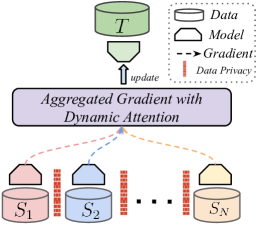
(a) Federated Domain Adaptation

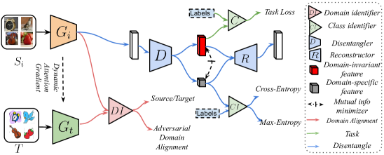
(b) Federated Adversarial Domain Adaptation

Figure 1: (a) We propose an approach for the UFDA setting, where data are not shareable between different domains. In our approach, models are trained separately on each source domain and their gradients are aggregated with dynamic attention mechanism to update the target model. (b) Our FADA model learns to extract domain-invariant features using adversarial domain alignment (red lines) and a feature disentangler (blue lines).

2 Related Work

Unsupervised Domain Adaptation Unsupervised Domain Adaptation (UDA) aims to transfer the knowledge learned from a labeled source domain to an unlabeled target domain. Domain adaptation approaches proposed over the past decade include discrepancy-based methods (Tzeng et al., 2014; Long et al., 2017; Ghifary et al., 2014; Sun & Saenko, 2016; Peng & Saenko, 2018), reconstruction-based UDA models (Yi et al., 2017; Zhu et al., 2017; Hoffman et al., 2018; Kim et al., 2017), and adversary-based approaches (Liu & Tuzel, 2016; Tzeng et al., 2017; Liu et al., 2018a; Ganin & Lempitsky, 2015). For example, Ganin & Lempitsky (2015) propose a gradient reversal layer to perform adversarial training to a domain discriminator, inspired by the idea of adversarial learning. Tzeng et al. (2017) address unsupervised domain adaptation by adapting a deep CNN-based feature extractor/classifier across source and target domains via adversarial training. Ben-David et al. (2010) introduce an $\mathcal{H}\Delta\mathcal{H}$-divergence to evaluate the domain shift and provide a generalization error bound for domain adaptation. These methods assume the data are centralized on one server, limiting their applicability to the distributed learning system.

Federated Learning Federated learning (Mohassel & Rindal, 2018; Rivest et al., 1978; Bonawitz et al., 2017; Mohassel & Zhang, 2017) is a decentralized learning approach which enables multiple clients to collaboratively learn a machine learning model while keeping the training data and model parameters on local devices. Inspired by Homomorphic Encryption (Rivest et al., 1978), Gilad-Bachrach et al. (2016) propose CryptoNets to enhance the efficiency of data encryption, achieving higher federated learning performance. Bonawitz et al. (2017) introduce a secure aggregation scheme to update the machine learning models under their federated learning framework. Recently, Mohassel & Zhang (2017) propose SecureML to support privacy-preserving collaborative training in a multi-client federated learning system. However, these methods mainly aim to learn a single global model across the data and have no convergence guarantee, which limits their ability to deal with non-i.i.d. data. To address the non-i.i.d data, Smith et al. (2017) introduce federated multi-task learning, which learns a separate model for each node. Liu et al. (2018b) propose semi-supervised federated transfer learning in a privacy-preserving setting. However, their models involve full or semi-supervision. The work proposed here is, to our best knowledge, the first federated learning framework to consider unsupervised domain adaptation.

Feature Disentanglement Deep neural networks are known to extract features where multiple hidden factors are highly entangled. Learning disentangled representations can help remove irrelevant and domain-specific features and model only the relevant factors of data variation. To this end, recent work (Mathieu et al., 2016; Makhzani et al., 2016; Liu et al., 2018a; Odena et al., 2017) explores the learning of interpretable representations using generative adversarial networks (GANs) (Goodfellow et al., 2014) and variational autoencoders (VAEs) (Kingma & Welling, 2013). Under the fully supervised setting, (Odena et al., 2017) propose an auxiliary classifier GAN (AC-GAN) to achieve representation disentanglement. (Liu et al., 2018a) introduce a unified feature disentanglement framework to learn domain-invariant features from data across different domains. (Kingma et al., 2014) also extend VAEs into the semi-supervised setting for representation disentanglement. (Lee et al., 2018) propose to disentangle the features into a domain-invariant content space and a domain-specific attributes space, producing diverse outputs without paired training data. Inspired by these works, we propose a method to disentangle the domain-invariant features from domain-specific features, using an adversarial training process. In addition, we propose to minimize the mutual information between the domain-invariant features and domain-specific features to enhance the feature disentanglement.

3 Generalization Bound for Federated Domain Adaptation

We first define the notation and review a typical theoretical error bound for single-source domain adaptation (Ben-David et al., 2007; Blitzer et al., 2008) devised by Ben-David et al. Then we describe our derived error bound for unsupervised federated domain adaptation. We mainly focus on the high-level interpretation of the error bound here and refer our readers to the appendix (see supplementary material) for proof details.

Notation. Let $\mathcal{D}_{S}$ and $\mathcal{D}_{T}$ denote source and target distribution on input space $\mathcal{X}$ and a ground-truth labeling function $g:\mathcal{X}\to\{0,1\}$. A hypothesis is a function $h:\mathcal{X}\to\{0,1\}$ with the error w.r.t the ground-truth labeling function $g$: $\epsilon_{S}(h,g):=\mathbb{E}_{\mathbf{x}\sim\mathcal{D}_{S}}[|h(\mathbf{x})-g(\mathbf{x})|]$. We denote the risk and empirical risk of hypothesis $h$ on $\mathcal{D}_{S}$ as $\epsilon_{S}(h)$ and $\widehat{\epsilon}_{S}(h)$. Similarly, the risk and empirical risk of $h$ on $\mathcal{D}_{T}$ are denoted as $\epsilon_{T}(h)$ and $\widehat{\epsilon}_{T}(h)$. The $\mathcal{H}$-divergence between two distributions $\mathcal{D}$ and $\mathcal{D}^{\prime}$ is defined as: $d_{\mathcal{H}}(\mathcal{D},\mathcal{D}^{\prime}):=2\sup_{A\in\mathcal{A}_{\mathcal{H}}}|\Pr_{\mathcal{D}}(A)-\Pr_{\mathcal{D}^{\prime}}(A)|$, where $\mathcal{H}$ is a hypothesis class for input space $\mathcal{X}$, and $\mathcal{A}_{\mathcal{H}}$ denotes the collection of subsets of $\mathcal{X}$ that are the support of some hypothesis in $\mathcal{H}$.

The symmetric difference space $\mathcal{H}\Delta\mathcal{H}$ is defined as: $\mathcal{H}\Delta\mathcal{H}:=\{h(\mathbf{x})\oplus h^{\prime}(\mathbf{x}))|h,h^{\prime}\in\mathcal{H}\}$, ($\oplus$: the XOR operation). We denote the optimal hypothesis that achieves the minimum risk on the source and the target as $h^{*}:=\arg\min_{h\in\mathcal{H}}\epsilon_{S}(h)+\epsilon_{T}(h)$ and the error of $h^{*}$ as $\lambda:=\epsilon_{S}(h^{*})+\epsilon_{T}(h^{*})$. Blitzer et al. (2007b) prove the following error bound on the target domain.

Theorem 1.

Let $\mathcal{H}$ be a hypothesis space of $VC$-dimension $d$ and $\widehat{\mathcal{D}}_{S}$, $\widehat{\mathcal{D}}_{T}$ be the empirical distribution induced by samples of size $m$ drawn from $\mathcal{D}_{S}$ and $\mathcal{D}_{T}$. Then with probability at least $1-\delta$ over the choice of samples, for each $h\in\mathcal{H}$,

$$\epsilon_{T}(h)\leq\widehat{\epsilon}_{S}(h)+\frac{1}{2}\widehat{d}_{\mathcal{H}\Delta\mathcal{H}}(\widehat{\mathcal{D}}_{S},\widehat{\mathcal{D}}_{T})+4\sqrt{\frac{2d\log(2m)+\log(4/\delta)}{m}}+\lambda$$ (1)

Let ${\mathcal{D}}_{S}$=$\{\mathcal{D}_{S_{i}}\}_{i=1}^{N}$, and ${\mathcal{D}}_{T}=\{\mathbf{x}_{j}^{t}\}_{j=1}^{n_{t}}$ be $N$ source domains and the target domain in a UFDA system, where $\mathcal{D}_{S_{i}}=\{(\mathbf{x}_{j}^{s},\mathbf{y}^{s}_{j})\}_{j=1}^{n_{i}}$. In federated domain adaptation system, $\mathcal{D}_{S}$ is distributed on $N$ nodes and the data are not shareable with each other in the training process. The classical domain adaptation algorithms aim to minimize the target risk $\epsilon_{T}(h):=\Pr_{(\mathbf{x},y)\sim\mathcal{D}_{T}}[h(\mathbf{x})\neq y]$. However, in a UFDA system, one model cannot directly get access to data stored on different nodes for security and privacy reasons. To address this issue, we propose to learn separate models for each distributed source domain $h_{S}=\{h_{S_{i}}\}_{i=1}^{N}$. The target hypothesis $h_{T}$ is the aggregation of the parameters of $h_{S}$, i.e. $h_{T}:=\sum_{i=1}^{N}{\alpha_{i}}{h_{S_{i}}}$, $\forall\alpha\in\mathbb{R}_{+}^{N}$, $\sum_{i\in[N]}\alpha_{i}=1$. We can then derive the following error bound:

Theorem 2.

(Weighted error bound for federated domain adaptation). Let $\mathcal{H}$ be a hypothesis class with VC-dimension d and $\{\widehat{\mathcal{D}}_{S_{i}}\}_{i=1}^{N}$, $\widehat{\mathcal{D}}_{T}$ be empirical distributions induced by a sample of size m from each source domain and target domain in a federated learning system, respectively. Then, $\forall\alpha\in\mathbb{R}_{+}^{N}$, $\sum_{i=1}^{N}{\alpha_{i}}=1$, with probability at least $1-\delta$ over the choice of samples, for each $h\in\mathcal{H}$,

$$\epsilon_{T}(h_{T})\leq\underbrace{\widehat{\epsilon}_{\tilde{S}}(\sum_{i\in[N]}\alpha_{i}h_{S_{i}})}_{\text{error on source }}+\sum_{i\in[N]}\alpha_{i}\bigg{(}\frac{1}{2}\underbrace{\widehat{d}_{\mathcal{H}\Delta\mathcal{H}}(\widehat{\mathcal{D}}_{S_{i}},\widehat{\mathcal{D}}_{T})}_{(\mathcal{D}_{S_{i}},\mathcal{D}_{T})\text{ divergence}}+\lambda_{i}\bigg{)}+\underbrace{4\sqrt{\frac{2d\log(2Nm)+\log(4/\delta)}{Nm}}}_{\text{VC-Dimension Constraint}}$$ (2)

where $\lambda_{i}$ is the risk of the optimal hypothesis on the mixture of $\mathcal{D}_{S_{i}}$ and $T$, and $\tilde{S}$ is the mixture of source samples with size $Nm$. $\widehat{d}_{\mathcal{H}\Delta\mathcal{H}}(\widehat{\mathcal{D}}_{S_{i}},\widehat{\mathcal{D}}_{T})$ denotes the divergence between domain $S_{i}$ and $T$.

Comparison with Existing Bounds The bound in (2) is extended from (1) and they are equivalent if only one source domain exists ($N=1$). Mansour et al. (2009) provide a generalization bound for multiple-source domain adaptation, assuming that the target domain is a mixture of the $N$ source domains. In contrast, in our error bound (2), the target domain is assumed to be an novel domain, resulting in a bound involving $\mathcal{H}\Delta\mathcal{H}$ discrepancy (Ben-David et al., 2010) and the VC-dimensional constraint (Vapnik & Vapnik, 1998). Blitzer et al. (2007b) propose a generalization bound for semi-supervised multi-source domain adaptation, assuming that partial target labels are available. Our generalization bound is devised for unsupervised learning. Zhao et al. (2018) introduce classification and regression error bounds for multi-source domain adaptation. However, these error bounds assume that the multiple source and target domains exactly share the same hypothesis. In contrast, our error bound involves multiple hypotheses.

4 Federated Adversarial Domain Adaptation

The error bound in Theorem (2) demonstrates the importance of the weight $\alpha$ and the discrepancy ${d}_{\mathcal{H}\Delta\mathcal{H}}({\mathcal{D}}_{S},{\mathcal{D}}_{T})$ in unsupervised federated domain adaptation. Inspired by this, we propose dynamic attention model to learn the weight $\alpha$ and federated adversarial alignment to minimize the discrepancy between the source and target domains, as shown in Figure 1. In addition, we leverage representation disentanglement to extract domain-invariant representations to further enhance knowledge transfer.

Dynamic Attention In a federated domain adaptation system, the models on different nodes have different convergence rates. In addition, the domain shifts between the source domains and target domain are different, leading to a phenomenon where some nodes may have no contribution or even negative transfer (Pan & Yang, 2010) to the target domain. To address this issue, we propose dynamic attention, which is a mask on the gradients from source domains. The philosophy behind the dynamic attention is to increase the weight of those nodes whose gradients are beneficial to the target domain and limit the weight of those whose gradients are detrimental to the target domain. Specifically, we leverage the gap statistics (Tibshirani et al., 2001) to evaluate how well the target features $f^{t}$ can be clustered with unsupervised clustering algorithms (K-Means). Assuming we have $k$ clusters, the gap statistics are computed as:

$$I=\sum_{r=1}^{k}\frac{1}{2n_{r}}\sum_{i,j\in C_{r}}||f_{i}^{t}-f_{j}^{t}||_{2}$$ (3)

where we have clusters $C_{1},C_{2},...,C_{k}$, with $C_{r}$ denoting the indices of observations in cluster $r$, and $n_{r}$=$|C_{r}|$. Intuitively, a smaller gap statistics value indicates the feature distribution has smaller intra-class variance. We measure the contribution of each source domain by the gap statistics gain between two consecutive iterations: $I_{i}^{gain}=I_{i}^{p-1}-I_{i}^{p}$ ($p$ indicating training step), denoting how much the clusters can be improved before and after the target model is updated with the $i$-th source model’s gradient. The mask on the gradients from source domains is defined as $Softmax$($I_{1}^{gain}$,$I_{2}^{gain}$,…,$I_{N}^{gain}$).

Federated Adversarial Alignment The performance of machine learning models degrades rapidly with the presence of domain discrepancy (Long et al., 2015). To address this issue, existing work (Hoffman et al., 2018; Tzeng et al., 2015) proposes to minimize the discrepancy with an adversarial training process. For example, Tzeng et al. (2015) proposes the domain confusion objective, under which the feature extractor is trained with a cross-entropy loss against a uniform distribution. However, these models require access to the source and target data simultaneously, which is prohibitive in UFDA. In the federated setting, we have multiple source domains and the data are locally stored in a privacy-preserving manner, which means we cannot train a single model which has access to the source domain and target domain simultaneously. To address this issue, we propose federated adversarial alignment that divides optimization into two independent steps, a domain-specific local feature extractor and a global discriminator. Specifically, (1) for each domain, we train a local feature extractor, $G_{i}$ for $\mathcal{D}_{i}$ and $G_{t}$ for $\mathcal{D}_{t}$, (2) for each ($\mathcal{D}_{i}$, $\mathcal{D}_{t}$) source-target domain pair, we train an adversarial domain identifier $DI$ to align the distributions in an adversarial manner: we first train $DI$ to identify which domain are the features come from, then we train the generator ($G_{i}$, $G_{t}$) to confuse the $DI$. Note that $D$ only gets access to the output vectors of $G_{i}$ and $G_{t}$, without violating the UFDA setting. Given the $i$-th source domain data $\mathbf{X}^{S_{i}}$, target data $\mathbf{X}^{T}$, the objective for $DI_{i}$ is defined as follows:

$${\color[rgb]{0,0,0}{\underset{\Theta^{DI_{i}}}{\mathcal{L}_{{adv}_{DI_{i}}}}(\mathbf{X}^{S_{i}},\mathbf{X}^{T},G_{i},G_{t})=-\mathbb{E}_{\mathbf{x}^{s_{i}}\sim\mathbf{X}^{s_{i}}}\left[\log DI_{i}(G_{i}(\mathbf{x}^{s_{i}}))]-\mathbb{E}_{\mathbf{x}^{t}\sim\mathbf{X}^{t}}[\log(1-DI_{i}(G_{t}(\mathbf{x}^{t})))\right]}}.$$ (4)

In the second step, $\mathcal{L}_{\text{adv}_{D}}$ remains unchanged, but $\mathcal{L}_{\text{adv}_{G}}$ is updated with the following objective:

$${\color[rgb]{0,0,0}{\underset{\Theta^{G_{i}},\Theta^{G_{t}}}{\mathcal{L}_{{adv}_{G}}}(\mathbf{X}^{S_{i}},\mathbf{X}^{T},DI_{i})=-\mathbb{E}_{\mathbf{x}^{s_{i}}\sim\mathbf{X}^{s_{i}}}[\log DI_{i}(G_{i}(\mathbf{x}^{s_{i}}))]-\mathbb{E}_{\mathbf{x}^{t}\sim\mathbf{X}^{t}}[\log DI_{i}(G_{t}(\mathbf{x}^{t}))]}}$$ (5)

Algorithm 1 Federated Adversarial Domain Adaptation

Input: $N$ source domains ${\mathcal{D}}_{S}$=$\{\mathcal{D}_{S_{i}}\}_{i=1}^{N}$; a target domain ${\mathcal{D}}_{t}=\{\mathbf{x}_{j}^{t}\}_{j=1}^{n_{t}}$; $N$ feature extractors $\{\Theta^{G_{1}},\Theta^{G_{2}},...\Theta^{G_{N}}\}$, $N$ disentanglers $\{\Theta^{D_{1}},\Theta^{D_{2}},...\Theta^{D_{N}}\}$, $N$ classifiers $\{\Theta^{C_{1}},\Theta^{C_{2}},...\Theta^{C_{N}}\}$, $N$ class identifiers $\{\Theta^{CI_{1}},\Theta^{CI_{2}},...\Theta^{CI_{N}}\}$, $N$ mutual information estimators $\{\Theta^{M_{1}},\Theta^{M_{2}},...\Theta^{M_{N}}\}$ trained on source domains. Target feature extractor $\Theta^{G_{t}}$, classifier $\Theta^{C_{t}}$. $N$ domain identifiers $\{\Theta^{DI_{1}},\Theta^{DI_{2}},...,\Theta^{DI_{N}}\}$

Output: well-trained target feature extractor $\hat{\Theta}^{G_{t}}$, target classifier $\hat{\Theta}^{C_{t}}$ .
 Model Initialization .

1:while not converged do

2:     for i do=1:N

3:         Sample mini-batch from from $\{(\mathbf{x}_{i}^{s},y^{s}_{i})\}_{i=1}^{n_{s}}$ and $\{\mathbf{x}_{j}^{t}\}_{j=1}^{n_{t}}$;

4:         Compute gradient with cross-entropy classification loss, update $\Theta^{G_{i}}$, $\Theta^{C_{i}}$.

5:         Domain Alignment:

6:         Update $\Theta^{DI_{i}}$, $\{\Theta^{G_{i}},\Theta^{G_{t}}\}$ with Eq. 4 and Eq. 5 respectively to align the domain distribution;

7:         Domain Disentangle:

8:         update $\Theta^{G_{i}},\Theta^{D_{i}},\Theta^{C_{i}},\Theta^{CI_{i}}$ with Eq. 6

9:         update $\Theta^{D_{i}}$ and $\{\Theta^{G_{i}}\}$ with Eq. 7

10:         Mutual Information Minimization:

11:         Calculate mutual information between the disentangled feature pair ($f_{di}$, $f_{ds}$) with $M_{i}$;

12:         Update $\Theta^{D_{i}}$, $\Theta^{M_{i}}$ by Eq.8;

13:     end for

14:     Dynamic weight:

15:     Calculate dynamic weight by Eq. 3

16:     Update $\Theta^{G_{t}},\Theta^{C_{t}}$ by aggregated $\{\Theta^{G_{1}},\Theta^{G_{2}},...,\Theta^{G_{N}}\}$, $\{\Theta^{C_{1}},\Theta^{C_{2}},...\Theta^{C_{N}}\}$ respectively with the computed dynamic weight;

17:end while

18:return $\Theta^{G_{t}}$, $\Theta^{C_{t}}$

Representation Disentanglement We employ adversarial disentanglement to extract the domain-invariant features. The high-level intuition is to disentangle the features extracted by ($G_{i}$, $G_{t}$) into domain-invariant and domain-specific features. As shown in Figure 1(b), the disentangler $D_{i}$ separates the extracted features into two branches. Specifically, we first train the $K$-way classifier $C_{i}$ and $K$-way class identifier $CI_{i}$ to correctly predict the labels with a cross-entropy loss, based on $f_{di}$ and $f_{ds}$ features, respectively. The objective is:

$${\color[rgb]{0,0,0}{\underset{\Theta^{G_{i}},\Theta^{D_{i}},\Theta^{C_{i}},\Theta^{CI_{i}}}{\mathcal{L}_{cross-entropy}}=-\mathbb{E}_{(\mathbf{x}^{s_{i}},\mathbf{y}^{s_{i}})\sim\widehat{\mathcal{D}}_{s_{i}}}\sum_{k=1}^{K}\mathds{1}[k=\mathbf{y}^{s_{i}}]log(C_{i}(f_{di}))-\mathbb{E}_{(\mathbf{x}^{s_{i}},\mathbf{y}^{s_{i}})\sim\widehat{\mathcal{D}}_{s_{i}}}\sum_{k=1}^{K}\mathds{1}[k=\mathbf{y}^{s_{i}}]log(CI_{i}(f_{ds}))}}$$ (6)

where $f_{di}=D_{i}(G_{i}(\mathbf{x^{s_{i}}}))$, $f_{ds}=D_{i}(G_{i}(\mathbf{x}^{s_{i}}))$ denote the domain-invariant and domain-specific features respectively. In the next step, we freeze the class identifier $CI_{i}$ and only train the feature disentangler to confuse the class identifier $CI_{i}$ by generating the domain-specific features $f_{ds}$, as shown in Figure 1. This can be achieved by minimizing the negative entropy loss of the predicted class distribution. The objective is as follows:

$${\color[rgb]{0,0,0}{\underset{\Theta^{D_{i}},\Theta^{G_{i}}}{\mathcal{L}_{ent}}=-\frac{1}{N_{s_{i}}}\sum_{j=1}^{N_{s_{i}}}\log CI_{i}(f^{j}_{ds})=-\frac{1}{N_{s_{i}}}\sum_{j=1}^{N_{s_{i}}}\log CI_{i}(D_{i}(G_{i}(\mathbf{x}^{s_{i}})))}}$$ (7)

Feature disentanglement facilitates the knowledge transfer by reserving $f_{di}$ and dispelling $f_{ds}$. To enhance the disentanglement, we minimize the mutual information between domain-invariant features and domain-specific features, following Peng et al. (2019). Specifically, the mutual information is defined as $I({f}_{di};{f}_{ds})=\int_{\mathcal{P}\times\mathcal{Q}}\log{\frac{d\mathbb{P}_{\mathcal{P}\mathcal{Q}}}{d\mathbb{P}_{\mathcal{P}}\otimes\mathbb{P}_{\mathcal{Q}}}}d\mathbb{P}_{\mathcal{P}\mathcal{Q}}$, where $\mathbb{P}_{\mathcal{P}\mathcal{Q}}$ is the joint probability distribution of (${f}_{di},{f}_{ds}$), and $\mathbb{P}_{\mathcal{P}}=\int_{\mathcal{Q}}d\mathbb{P}_{\mathcal{P}\mathcal{Q}}$, $\mathbb{P}_{\mathcal{Q}}=\int_{\mathcal{Q}}d\mathbb{P}_{\mathcal{P}\mathcal{Q}}$ are the marginals. Despite being a pivotal measure across different distributions, the mutual information is only tractable for discrete variables, for a limited family of problems where the probability distributions are unknown (Belghazi et al., 2018). Following Peng et al. (2019), we adopt the Mutual Information Neural Estimator (MINE) (Belghazi et al., 2018) to estimate the mutual information by leveraging a neural network $T_{\theta}$: $\widehat{I(\mathcal{P};\mathcal{Q})}_{n}=\sup_{\theta\in\Theta}\mathbb{E}_{\mathbb{P}^{(n)}_{\mathcal{P}\mathcal{Q}}}[T_{\theta}]-\log(\mathbb{E}_{\mathbb{P}^{(n)}_{\mathcal{P}}\otimes\widehat{\mathbb{P}}^{(n)}_{\mathcal{Q}}}[e^{T_{\theta}}])$. Practically, MINE can be calculated as $I(\mathcal{P};\mathcal{Q})=\int\int{\mathbb{P}^{n}_{\mathcal{P}\mathcal{Q}}(p,q)\text{ }T(p,q,\theta)}$ - $\log(\int\int\mathbb{P}^{n}_{\mathcal{P}}(p)\mathbb{P}^{n}_{\mathcal{Q}}(q)e^{T(p,q,\theta)})$. To avoid computing the integrals, we leverage Monte-Carlo integration to calculate the estimation:

$$I(\mathcal{P},\mathcal{Q})=\frac{1}{n}\sum^{n}_{i=1}T(p,q,\theta)-\log(\frac{1}{n}\sum_{i=1}^{n}e^{T(p,q^{\prime},\theta)})$$ (8)

where $(p,q)$ are sampled from the joint distribution, $q^{\prime}$ is sampled from the marginal distribution, and $T(p,q,\theta)$ is the neural network parameteralized by $\theta$ to estimate the mutual information between $\mathcal{P}$ and $\mathcal{Q}$, we refer the reader to MINE (Belghazi et al., 2018) for more details. The domain-invariant and domain-specific features are forwarded to a reconstructor with a L2 loss to reconstruct the original features, aming to keep the representation integrity, as shown in Figure 1(b). The balance of the L2 reconstruction and mutual information can be achieved by adjusting the hyper-parameters of the L2 loss and mutual information loss.

Optimization Our model is trained in an end-to-end fashion. We train federated alignment and representation disentanglement component with Stochastic Gradient Descent (Kiefer et al., 1952). The federated adversarial alignment loss and representation disentanglement loss are minimized together with the task loss. The detailed training procedure is presented in Algorithm 1.

5 Experiments

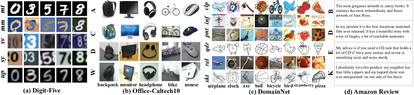
Figure 2: We demonstrate the effectiveness of FADA on four datasets: (1) “Digit-Five”, which includes MNIST (mt), MNIST-M (mm), SVHN (sv), Synthetic (syn), and USPS (up). (2) Office-Caltech10 dataset, which contains Amazon (A), Caltech (C), DSLR (D), and Webcam (W). (3) DomainNet dataset, which includes: clipart (clp), infograph (inf), painting (pnt), quickdraw (qdr), real (rel), and sktech (skt). (4) Amazon Review dataset, which contains review for Books (B), DVDs (D), Electronics (E), and Kitchen & housewares (K).

We test our model on the following tasks: digit classification (Digit-Five), object recognition (Office-Caltech10 (Gong et al., 2012), DomainNet (Peng et al., 2018)) and sentiment analysis (Amazon Review dataset (Blitzer et al., 2007a)). Figure 2 shows some data samples and Table 10 (see supplementary material) shows the number of data per domain we used in our experiments. We perform our experiments on a 10 Titan-Xp GPU cluster and simulate the federated system on a single machine (as the data communication is not the main focus of this paper). Our model is implemented with PyTorch. We repeat every experiment 10 times on the Digit-Five and Amazon Review datasets, and 5 times on the Office-Caltech10 and DomainNet (Peng et al., 2018) datasets, reporting the mean and standard derivation of accuracy. To better explore the effectiveness of different components of our model, we propose three different ablations, i.e. model I: with dynamic attention; model II: I + adversarial alignment; and model III: II + representation disentanglement.

5.1 Experiments on Digit Recognition

Digit-Five This dataset is a collection of five benchmarks for digit recognition, namely MNIST (LeCun et al., 1998), Synthetic Digits (Ganin & Lempitsky, 2015), MNIST-M (Ganin & Lempitsky, 2015), SVHN, and USPS. In our experiments, we take turns setting one domain as the target domain and the rest as the distributed source domains, leading to five transfer tasks. The detailed architecture of our model can be found in Table 7 (see supplementary material).

Since many DA models (Saito et al., 2018; French et al., 2018; Hoffman et al., 2018) require access to data from different domains, it is infeasible to directly compare our model to these baselines. Instead, we compare our model to the following popular domain adaptation baselines: Domain Adversarial Neural Network (DANN) (Ganin & Lempitsky, 2015), Deep Adaptation Network (DAN) (Long et al., 2015), Automatic DomaIn Alignment Layers (AutoDIAL) (Carlucci et al., 2017), and Adaptive Batch Normalization (AdaBN) Li et al. (2016). Specifically, DANN minimizes the domain gap between source domain and target domain with a gradient reversal layer. DAN applies multi-kernel MMD loss (Gretton et al., 2007) to align the source domain with the target domain in Reproducing Kernel Hilbert Space. AutoDIAL introduces domain alignment layer to deep models to match the source and target feature distributions to a reference one. AdaBN applies Batch Normalization layer (Ioffe & Szegedy, 2015) to facilitate the knowledge transfer between the source and target domains. When conducting the baseline experiments, we use the code provided by the authors and modify the original settings to fit federated DA setting (i.e. each domain has its own model), denoted by $f$-DAN and $f$-DANN. In addition, to demonstrate the difficulty of UFDA where accessing all source data with a single model is prohibative, we also perform the corresponding multi-source DA experiments (shared source data).

Models	mt,sv,sy,up$\rightarrow$mm	mm,sv,sy,up$\rightarrow$mt	mt,mm,sy,up$\rightarrow$sv	mt,mm,sv,up$\rightarrow$sy	mt,mm,sv,sy$\rightarrow$up	Avg
Source Only	63.3$\pm$0.7	90.5$\pm$0.8	88.7$\pm$0.8	63.5$\pm$0.9	82.4$\pm$0.6	77.7
DAN	63.7$\pm$0.7	96.3$\pm$0.5	94.2$\pm$0.8	62.4$\pm$0.7	85.4$\pm$0.7	80.4
DANN	71.3$\pm$0.5	97.6$\pm$0.7	92.3$\pm$0.8	63.4$\pm$0.7	85.3$\pm$0.8	82.1
Source Only	49.6$\pm$0.8	75.4$\pm$1.3	22.7$\pm$0.9	44.3$\pm$0.7	75.5$\pm$1.4	53.5
AdaBN	59.3$\pm$0.8	75.3$\pm$0.7	34.2$\pm$0.6	59.7$\pm$0.7	87.1$\pm$0.9	61.3
AutoDIAL	60.7$\pm$1.6	76.8$\pm$0.9	32.4$\pm$0.5	58.7$\pm$1.2	90.3$\pm$0.9	65.8
f-DANN	59.5$\pm$0.6	86.1$\pm$1.1	44.3 $\pm$0.6	53.4$\pm$0.9	89.7$\pm$0.9	66.6
f-DAN	57.5 $\pm$0.8	86.4 $\pm$0.7	45.3$\pm$0.7	58.4$\pm$0.7	90.8 $\pm$1.1	67.7
FADA+attention (I)	44.2$\pm$0.7	90.5$\pm$0.8	27.8$\pm$0.5	55.6$\pm$0.8	88.3$\pm$1.2	61.3
FADA+adversarial (II)	58.2$\pm$0.8	92.5$\pm$ 0.9	48.3$\pm$0.6	62.1$\pm$0.5	90.6$\pm$1.1	70.3
FADA+disentangle (III)	62.5$\pm$0.7	91.4 $\pm$0.7	50.5 $\pm$0.3	71.8$\pm$0.5	91.7$\pm$1.0	73.6

Table 1: Accuracy (%) on “Digit-Five” dataset with UFDA protocol. FADA achieves 73.6%, outperforming other baselines. We incrementally add each component t our model, aiming to study their effectiveness on the final results. (model I: with dynamic attention; model II: I+adversarial alignment; model III: II+representation disentanglement. mt, up, sv, sy, mm are abbreviations for MNIST, USPS, SVHN, Synthetic Digits, MNIST-M.)

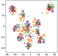
(a) Source Features

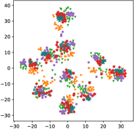
(b) f-DANN Features

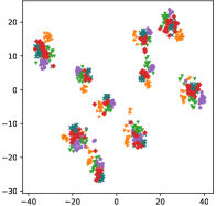
(c) f-DAN Features

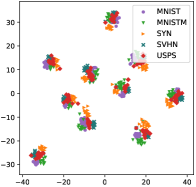
(d) FADA Features

Figure 3: Feature visualization: t-SNE plot of source-only features, f-DANN (Ganin & Lempitsky, 2015) features, f-DAN (Long et al., 2015) features and FADA features in sv,mm,mt,sy$\rightarrow$up setting. We use different markers and colors to denote different domains. The data points from target domain have been denoted by red for better visual effect. (Best viewed in color.)

Results and Analysis The experimental results are shown in Table 1. From the results, we can make the following observations. (1) Model III achieves 73.6% average accuracy, significantly outperforming the baselines. (2) The results of model I and model II demonstrate the effectiveness of dynamic attention and adversarial alignment. (3) Federated DA displays much weaker results than multi-source DA, demonstrating that the newly proposed UFDA learning setting is very challenging.

To dive deeper into the feature representation of our model versus other baselines, we plot in Figure 3(a)-3(d) the t-SNE embeddings of the feature representations learned on mm,mt,sv,sy$\rightarrow$up task with source-only features, $f$-DANN features, $f$-DAN features and FADA features, respectively. We observe that the feature embeddings of our model have smaller intra-class variance and larger inter-class variance than $f$-DANN and $f$-DAN, demonstrating that our model is capable of generating the desired feature embedding and can extract domain-invariant features across different domains.

5.2 Experiments on Office-Caltech10

Office-Caltech10 (Gong et al., 2012) This dataset contains 10 common categories shared by Office-31 (Saenko et al., 2010) and Caltech-256 datasets (Griffin et al., 2007). It contains four domains: Caltech (C), which are sampled from Caltech-256 dataset, Amazon (A), which contains images collected from amazon.com, Webcam (W) and DSLR (D), which contains images taken by web camera and DSLR camera under office environment.

Method	C,D,W $\rightarrow$ A	A,D,W $\rightarrow$ C	A,C,W $\rightarrow$ D	A,C,D $\rightarrow$ W	Average
AlexNet	80.1$\pm$0.4	86.9$\pm$0.3	82.7$\pm$0.5	85.1$\pm$0.3	83.7
$f$-DAN	82.5$\pm$0.5	87.2$\pm$0.4	85.6$\pm$0.4	86.1$\pm$0.3	85.4
$f$-DANN	83.1$\pm$0.4	86.5$\pm$0.5	84.8$\pm 0.5$	86.4$\pm$0.5	85.2
FADA+attention (I)	81.2$\pm$0.3	87.1$\pm$0.6	83.5$\pm 0.5$	85.9$\pm$0.4	84.4
FADA+adversarial (II)	83.1$\pm$0.6	87.8$\pm$0.4	85.4$\pm 0.4$	86.8$\pm$0.5	85.8
FADA+disentangle (III)	84.3$\pm$0.6	88.4$\pm$0.5	86.1$\pm$0.4	87.3$\pm$0.5	86.5
ResNet101	81.9$\pm$0.5	87.9$\pm$0.3	85.7$\pm$0.5	86.9$\pm$0.4	85.6
AdaBN	82.2$\pm$0.4	88.2$\pm$0.6	85.9$\pm$0.7	87.4$\pm$0.8	85.7
AutoDIAL	83.3$\pm$0.6	87.7$\pm$0.8	85.6$\pm$0.7	87.1$\pm$0.6	85.9
$f$-DAN	82.7$\pm$0.3	88.1$\pm$0.5	86.5$\pm$0.3	86.5$\pm$0.3	85.9
$f$-DANN	83.5$\pm$0.4	88.5$\pm$0.3	85.9$\pm$0.5	87.1$\pm$0.4	86.3
FADA+attention (I)	82.1$\pm$0.5	87.5$\pm$0.3	85.8$\pm$0.4	87.3$\pm$0.5	85.7
FADA+adversarial (II)	83.2$\pm$0.4	88.4$\pm$0.3	86.4$\pm$0.5	87.8$\pm$0.4	86.5
FADA+disentangle (III)	84.2$\pm$0.5	88.7$\pm$0.5	87.1$\pm$0.6	88.1$\pm$0.4	87.1

Table 2: Accuracy on Office-Caltech10 dataset with unsupervised federated domain adaptation protocol. The upper table shows the results for AlexNet backbone and the table below shows the results for ResNet backbone.

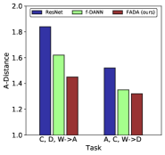
(a) $\mathcal{A}$-Distance

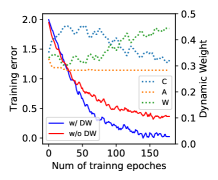
(b) Training loss for A,C,W$\rightarrow$D

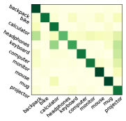
(c) $f$-DAN confusion matrix

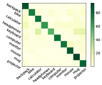
(d) FADA confusion matrix

Figure 4: (a)$\mathcal{A}$-Distance of ResNet, $f$-DANN, and FADA features on two different tasks. (b) training errors and dynamic weight on A,C,W$\rightarrow$D task. (c)-(d) confusion matrices of $f$-DAN, and FADA on A,C,D$\rightarrow$W task.

Models	inf,pnt,qdr, rel,skt$\rightarrow$clp	clp,pnt,qdr, rel,skt$\rightarrow$inf	clp,inf,qdr, rel,skt$\rightarrow$pnt	clp,inf,pnt, rel,skt$\rightarrow$qdr	clp,inf,pnt, qdr,skt$\rightarrow$rel	clp,inf,pnt, qdr,rel$\rightarrow$skt	Avg
AlexNet	39.2$\pm$0.7	12.7$\pm$0.4	32.7$\pm$0.4	5.9$\pm$0.7	40.3$\pm$0.5	22.7$\pm$0.6	25.6
$f$-DAN	41.6$\pm$0.6	13.7$\pm$0.5	36.3$\pm$0.5	6.5$\pm$0.5	43.5$\pm$0.8	22.9$\pm$0.5	27.4
$f$-DANN	42.6$\pm$0.8	14.1$\pm$0.7	35.2$\pm$0.3	6.2$\pm$0.7	42.9$\pm$0.5	22.7$\pm$0.7	27.2
FADA+disentangle (III)	44.9$\pm$0.7	15.9$\pm$0.6	36.3$\pm$0.8	8.6$\pm$0.8	44.5$\pm$0.6	23.2$\pm$0.8	28.9
ResNet101	41.6 $\pm$0.6	14.5$\pm$0.7	35.7$\pm$0.7	8.4$\pm$0.7	43.5$\pm$0.7	23.3$\pm$0.7	27.7
$f$-DAN	43.5$\pm$0.7	14.1$\pm$0.6	37.6$\pm$0.7	8.3$\pm$0.6	44.5$\pm$0.5	25.1$\pm$0.5	28.9
$f$-DANN	43.1$\pm$0.8	15.2$\pm$0.9	35.7$\pm$0.4	8.2$\pm$0.6	45.2$\pm$0.7	27.1$\pm$0.6	29.1
FADA+disentangle (III)	45.3$\pm$0.7	16.3$\pm$0.8	38.9 $\pm$0.7	7.9$\pm$0.4	46.7$\pm$0.4	26.8$\pm$0.4	30.3

Table 3: Accuracy (%) on the DomainNet dataset (Peng et al., 2018) dataset under UFDA protocol. The upper table shows the results based on AlexNet (Krizhevsky et al., 2012) backbone and the table below are the results based on ResNet (He et al., 2016) backbone.

Method	D,E,K $\rightarrow$ B	B,E,K $\rightarrow$ D	B,D,K $\rightarrow$ E	B,D,E $\rightarrow$ K	Average
Source Only	74.4$\pm 0.3$	79.2$\pm$0.4	73.5 $\pm$0.2	71.4$\pm$0.1	74.6
$f$-DANN	75.2$\pm$0.3	82.7$\pm$0.2	76.5$\pm$0.3	72.8$\pm$0.4	76.8
AdaBN	76.7$\pm$0.3	80.9$\pm$0.3	75.7$\pm$0.2	74.6$\pm$0.3	76.9
AutoDIAL	76.3$\pm$0.4	81.3$\pm$0.5	74.8$\pm$0.4	75.6$\pm$0.2	77.1
$f$-DAN	75.6$\pm$0.2	81.6$\pm$0.3	77.9$\pm$0.1	73.2$\pm$0.2	77.6
FADA+attention (I)	74.8$\pm$0.2	78.9$\pm$0.2	74.5$\pm$0.3	72.5$\pm$0.2	75.2
FADA+adversarial (II)	79.7$\pm$0.2	81.1$\pm$0.1	77.3$\pm$0.2	76.4$\pm$0.2	78.6
FADA+disentangle (III)	78.1$\pm$0.2	82.7$\pm$0.1	77.4$\pm$0.2	77.5$\pm$0.3	78.9

Table 4: Accuracy (%) on “Amazon Review” dataset with unsupervised federated domain adaptation protocol.

We leverage two popular networks as the backbone of feature generator $G$, i.e. AlexNet (Krizhevsky et al., 2012) and ResNet (He et al., 2016). Both the networks are pre-trained on ImageNet (Deng et al., 2009). Other components of our model are randomly initialized with the normal distribution. In the learning process, we set the learning rate of randomly initialized parameters to ten times of the pre-trained parameters as it will take more time for those parameters to converge. Details of our model are listed in Table 9 (supplementary material).

Results and Analysis The experimental results on Office-Caltech10 datasets are shown in Table 2. We utilize the same backbones as the baselines and separately show the results. We make the following observations from the results: (1) Our model achieves 86.5% accuracy with an AlexNet backbone and 87.1% accuracy with a ResNet backbone, outperforming the compared baselines. (2) All the models have similar performance when C,D,W are selected as the target domain, but perform worse when A is selected as the target domain. This phenomenon is probably caused by the large domain gap, as the images in A are collected from amazon.com and contain a white background.

To better analyze the effectiveness of FADA, we perform the following empirical analysis: (1) $\mathcal{A}$-distance Ben-David et al. (2010) suggests $\mathcal{A}$-distance as a measure of domain discrepancy. Following Long et al. (2015), we calculate the approximate $\mathcal{A}$-distance ${\hat{d}_{\cal A}}=2\left({1-2\epsilon}\right)$ for C,D,W$\rightarrow$A and A,C,W$\rightarrow$D tasks, where $\epsilon$ is the generalization error of a two-sample classifier (e.g. kernel SVM) trained on the binary problem of distinguishing input samples between the source and target domains. In Figure 4(a), we plot for tasks with raw ResNet features, $f$-DANN features, and FADA features, respectively. We observe that the ${\hat{d}_{\cal A}}$ on DADA features are smaller than ResNet features and $f$-DANN features, demonstrating that FADA features are harder to be distinguished between source and target. (2) To show how the dynamic attention mechanism benefits the training process, we plot the training loss w/ or w/o dynamic weights for A,C,W$\rightarrow$D task in Figure 4(b). The figure shows the target model’s training error is much smaller when dynamic attention is applied, which is consistent with the quantitative results. In addition, in A,C,W$\rightarrow$D setting, the weight of A decreases to the lower bound after first a few epochs and the weight of W increases during the training process, as photos in both D and W are taken in the same environment with different cameras. (3) To better analyze the error mode, we plot the confusion matrices for $f$-DAN and FADA on A,C,D->W task in Figure 4(c)-4(d). The figures show that $f$-DAN mainly confuses ”calculator” vs. “keyboard”, “backpack” with “headphones”, while FADA is able to distinguish them with disentangled features.

5.3 Experiments on DomainNet

DomainNet  This dataset contains approximately 0.6 million images distributed among 345 categories. It comprises of six domains: Clipart (clp), a collection of clipart images; Infograph (inf), infographic images with specific object; Painting (pnt), artistic depictions of object in the form of paintings; Quickdraw (qdr), drawings from the worldwide players of game “Quick Draw!"; Real (rel, photos and real world images; and Sketch (skt), sketches of specific objects. This dataset is very large-scale and contains rich and informative vision cues across different domains, providing a good testbed for unsupervised federated domain adaptation. Some sample images can be found in Figure 2.

Results The experimental results on DomainNet are shown in Table 5.2. Our model achieves 28.9% and 30.3% accuracy with AlexNet and ResNet backbone, respectively. In both scenarios, our model outperforms the baselines, demonstrating the effectiveness of our model on large-scale dataset. Note that this dataset contains about 0.6 million images, and so even a one-percent performance improvement is not trivial. From the experiment results, we can observe that all the models deliver less desirable performance when infograph and quickdraw are selected as the target domains. This phenomenon is mainly caused by the large domain shift between inf/qdr domain and other domains.

5.4 Experiments on Amazon Review

Amazon Review (Blitzer et al., 2007a) This dataset provides a testbed for cross-domain sentimental analysis of text. The task is to identify whether the sentiment of the reviews is positive or negative. The dataset contains reviews from amazon.com users for four popular merchandise categories: Books (B), DVDs (D), Electronics (E), and Kitchen appliances (K). Following Gong et al. (2013), we utilize 400-dimensional bag-of-words representation and leverage a fully connected deep neural network as the backbone. The detailed architecture of our model can be found in Table 8 (supplementary materials).

Results The experimental results on Amazon Review dataset are shown in Table 4. Our model achieves an accuracy of 78.9% and outperforms the compared baselines. We make two major observations from the results: (1) Our model is not only effective on vision tasks but also performs well on linguistic tasks under UFDA learning schema. (2) From the results of model I and II, we can observe the dynamic attention and federated adversarial alignment are beneficial to improve the performance. However, the performance boost from Model II to Model III is limited. This phenomenon shows that the linguistic features are harder to disentangle comparing to visual features.

5.5 Ablation Study

To demonstrate the effectiveness of dynamic attention, we perform the ablation study analysis. The Table 5 shows the results on “Digit-Five”, Office-Caltech10 and Amazon Review benchmark. We observe that the performance drops in most of the experiments when dynamic attention model is not applied. The dynamic attention model is devised to cope with the varying convergence rates in the federated learning system, i.e., different source domains have their own convergence rate. In addition, it will increase the weight of a specific domain when the domain shift between that domain and the target domain is small, and decrease the weight otherwise.

target	mm	mt	sv	sy	up	Avg	A	C	D	W	Avg	B	D	E	K	Avg
FADA w/o. attention	60.1	91.2	49.2	69.1	90.2	71.9	83.3	85.7	86.2	88.3	85.8	77.2	82.8	77.2	76.3	78.3
FADA w. attention	62.5	91.4	50.5	71.8	91.7	73.6	84.2	88.7	87.1	88.1	87.1	78.1	82.7	77.4	77.5	78.9

Table 5: The ablation study results show that the dynamic attention module is essential for our model.

6 Conclusion

In this paper, we first proposed a novel unsupervised federated domain adaptation (UFDA) problem and derived a theoretical generalization bound for UFDA. Inspired by the theoretical results, we proposed a novel model called Federated Adversarial Domain Adaptation (FADA) to transfer the knowledge learned from distributed source domains to an unlabeled target domain with a novel dynamic attention schema. Empirically, we showed that feature disentanglement boosts the performance of FADA in UFDA tasks. An extensive empirical evaluation on UFDA vision and linguistic benchmarks demonstrated the efficacy of FADA against several domain adaptation baselines.

7 Notations

We provide the explanations of notations occurred in this paper.

Notations	Name	Details
$DI$	domain identifier	align the domain pair ($G_{i}$,$G_{t}$)
$D$	disentangler	disentangle the feature to $f_{di}$ and feature $f_{ds}$.
$C$	classifier	predict the labels for input features
$CI$	class identify	extract domain-specific features.
$G_{i}$	feature generator	extract features for $\mathcal{D}_{S_{i}}$
$G_{t}$	feature generator	extract features for ${\mathcal{D}}_{t}$
$M$	mutual information estimator	estimate the mutual information between $f_{ds}$ and $f_{di}$

Table 6: Notations occurred in the paper.

8 Model Architecture

We provide the detailed model architecture (Table 7 and Table 9) for each component in our model: Generator, Disentangler, Domain Classifier, Classifier and MINE.

layer	configuration
Feature Generator
1	Conv2D (3, 64, 5, 1, 2), BN, ReLU, MaxPool
2	Conv2D (64, 64, 5, 1, 2), BN, ReLU, MaxPool
3	Conv2D (64, 128, 5, 1, 2), BN, ReLU
Disentangler
1	FC (8192, 3072), BN, ReLU
2	DropOut (0.5), FC (3072, 2048), BN, ReLU
Domain Identifier
1	FC (2048, 256), LeakyReLU
2	FC (256, 2), LeakyReLU
Class Identifier
1	FC (2048, 10), BN, Softmax
Reconstructor
1	FC (4096, 8192)
Mutual Information Estimator
fc1_x	FC (2048, 512), LeakyReLU
fc1_y	FC (2048, 512), LeakyReLU
2	FC (512,1)

Table 7: Model architecture for digit recognition task (“Digit-Five” dataset). For each convolution layer, we list the input dimension, output dimension, kernel size, stride, and padding. For the fully-connected layer, we provide the input and output dimensions. For drop-out layers, we provide the probability of an element to be zeroed.

layer	configuration
Feature Generator
1	FC (400, 128), BN, ReLU
Disentangler
1	FC (128, 64), BN, ReLU
2	DropOut (0.5), FC (64, 32), BN, ReLU
Domain Identifier
1	FC (64, 32), LeakyReLU
2	FC (32, 2), LeakyReLU
Class Identifier
1	FC (32, 2), BN, Softmax
Reconstructor
1	FC (64, 128)
Mutual Information Estimator
fc1_x	FC (32, 16), LeakyReLU
fc1_y	FC (32, 16), LeakyReLU
2	FC (16,1)

Table 8: Model architecture for cross-doman sentimental analysis task (“Amazon Review” dataset (Blitzer et al., 2007a)). For the fully-connected layers (FC), we provide the input and output dimensions. For drop-out layers (Dropout), we provide the probability of an element to be zeroed.

layer	configuration
Feature Generator: ResNet101 or AlexNet
Disentangler
1	Dropout(0.5), FC (2048, 2048), BN, ReLU
2	Dropout(0.5), FC (2048, 2048), BN, ReLU
Domain Identifier
1	FC (2048, 256), LeakyReLU
2	FC (256, 2), LeakyReLU
Class Identifier
1	FC (2048, 10), BN, Softmax
Reconstructor
1	FC (4096, 2048)
Mutual Information Estimator
fc1_x	FC (2048, 512), LeakyReLU
fc1_y	FC (2048, 512), LeakyReLU
2	FC (512,1)

Table 9: Model architecture for image recognition task (Office-Caltech10 (Gong et al., 2012) and DomainNet (Peng et al., 2018)). For each convolution layer, we list the input dimension, output dimension, kernel size, stride, and padding. For the fully-connected layer, we provide the input and output dimensions. For drop-out layers, we provide the probability of an element to be zeroed.

9 Details of datasets

We provide the detailed information of datasets. For Digit-Five and DomainNet, we provide the train/test split for each domain. For Office-Caltech10, we provide the number of images in each domain. For Amazon review dataset, we show the detailed number of positive reviews and negative reviews for each merchandise category.

Digit-Five
Splits	mnist	mnist_m	svhn	syn	usps		Total
Train	25,000	25,000	25,000	25,000	7,348		107,348
Test	9,000	9,000	9,000	9,000	1,860		37,860
Office-Caltech10
Splits		Amazon	Caltech	Dslr	Webcam		Total
Total		958	1,123	157	295		2,533
DomainNet
Splits	clp	inf	pnt	qdr	rel	skt	Total
Train	34,019	37,087	52,867	120,750	122,563	49,115	416,401
Test	14,818	16,114	22,892	51,750	52,764	21,271	179,609
Amazon Review
Splits		Books	DVDs	Electronics	Kitchen		Total
Positive		1,000	1,000	1,000	1,000		4,000
Negative		1,000	1,000	1,000	1,000		4,000

Table 10: Detailed number of samples we used in our experiments.

10 Proof of Theorem 2

Theorem 3.

(Weighted error bound for federated domain adaptation). Let $\mathcal{H}$ be a hypothesis class with VC-dimension d and $\{\widehat{\mathcal{D}}_{S_{i}}\}_{i=1}^{N}$, $\widehat{\mathcal{D}}_{T}$ be empirical distributions induced by a sample of size m from each source domain and target domain in a federated learning system, respectively. Then, $\forall\alpha\in\mathbb{R}_{+}^{N}$, $\sum_{i=1}^{N}{\alpha_{i}}=1$, with probability at least $1-\delta$ over the choice of samples, for each $h\in\mathcal{H}$,

$$\epsilon_{T}(h_{T})\leq\underbrace{\widehat{\epsilon}_{\tilde{S}}(\sum_{i\in[N]}\alpha_{i}h_{S_{i}})}_{\text{error on source }}+\sum_{i\in[N]}\alpha_{i}\bigg{(}\frac{1}{2}\underbrace{\widehat{d}_{\mathcal{H}\Delta\mathcal{H}}(\widehat{\mathcal{D}}_{S_{i}},\widehat{\mathcal{D}}_{T})}_{(\mathcal{D}_{S_{i}},\mathcal{D}_{T})\text{ divergence}}+\lambda_{i}\bigg{)}+\underbrace{4\sqrt{\frac{2d\log(2Nm)+\log(4/\delta)}{Nm}}}_{\text{VC-Dimension Constraint}}$$ (9)

where $\lambda_{i}$ is the risk of the optimal hypothesis on the mixture of $\mathcal{D}_{S_{i}}$ and $T$, and $\tilde{S}$ is the mixture of source samples with size $Nm$.

Proof.

Consider a combined source domain which is equivalent to a mixture distribution of the $N$ source domains, with the mixture weight $\alpha$, where $\alpha\in\mathbb{R}_{+}^{N}$ and $\sum_{i=1}^{N}{\alpha_{i}}=1$. Denote the mixture source domain distribution as $\tilde{D}_{S}^{\alpha}$ (where $\tilde{D}_{S}^{\alpha}:=\sum_{i\in[N]}\alpha_{i}\mathcal{D}_{S_{i}}$), and the data sampled from $\tilde{D}_{S}^{\alpha}$ as $\tilde{S}$. Theoretically, we can assume $\tilde{D}_{S}^{\alpha}$ and $\mathcal{D}_{T}$ to be the source domain and target domain, respectively. Apply Theorem 1, we have that for $0<\delta<1$, with probability of at least 1-$\delta$ over the choice of samples, for each $h\in\mathcal{H}$,

$$\epsilon_{T}(h)\leq\widehat{\epsilon}_{\tilde{S}}(h)+\frac{1}{2}\widehat{d}_{\mathcal{H}\Delta\mathcal{H}}(\widehat{\mathcal{D}}_{\tilde{S}},\widehat{\mathcal{D}}_{T})+4\sqrt{\frac{2d\log(2Nm)+\log(4/\delta)}{Nm}}+\lambda_{\alpha}$$ (10)

where $\lambda_{\alpha}$ is the risk of optimal hypothesis on the $\tilde{S}$ and $T$. The upper bound of $\widehat{d}_{\mathcal{H}\Delta\mathcal{H}}(\widehat{\mathcal{D}}_{\tilde{S}},\widehat{\mathcal{D}}_{T})$ can be derived as follows:

$$\widehat{d}_{\mathcal{H}\Delta\mathcal{H}}(\widehat{\mathcal{D}}_{\tilde{S}},\widehat{\mathcal{D}}_{T}) =2\sup_{A\in\mathcal{A}_{\mathcal{H}\Delta\mathcal{H}}}|\Pr_{\widehat{\mathcal{D}}_{\tilde{S}}}(A)-\Pr_{\widehat{\mathcal{D}}_{T}}(A)|$$

$$=2\sup_{A\in\mathcal{A}_{\mathcal{H}\Delta\mathcal{H}}}|\sum_{i\in[N]}\alpha_{i}\Big{(}\Pr_{\widehat{\mathcal{D}}_{\tilde{S_{i}}}}(A)-\Pr_{\widehat{\mathcal{D}}_{T}}(A)\Big{)}|$$

$$\leqslant 2\sup_{A\in\mathcal{A}_{\mathcal{H}\Delta\mathcal{H}}}\sum_{i\in[N]}\alpha_{i}\Big{(}|\Pr_{\widehat{\mathcal{D}}_{\tilde{S_{i}}}}(A)-\Pr_{\widehat{\mathcal{D}}_{T}}(A)\Big{)}|$$

$$\leqslant 2\sum_{i\in[N]}\alpha_{i}\sup_{A\in\mathcal{A}_{\mathcal{H}\Delta\mathcal{H}}}\Big{(}|\Pr_{\widehat{\mathcal{D}}_{\tilde{S_{i}}}}(A)-\Pr_{\widehat{\mathcal{D}}_{T}}(A)\Big{)}|$$

$$=\sum_{i\in[N]}\alpha_{i}\widehat{d}_{\mathcal{H}\Delta\mathcal{H}}(\widehat{\mathcal{D}}_{S_{i}},\widehat{D}_{T})$$

the first inequality is derived by the triangle inequality. Similarly, with the triangle inequality property, we can derive $\lambda_{\alpha}\leqslant\sum_{i\in[N]}\alpha_{i}\lambda_{i}$. On the other hand, for $\forall h_{T}\in\mathcal{H}$, we have: $\widehat{\epsilon}_{\tilde{S}}(h_{T})=\widehat{\epsilon}_{\tilde{S}}(\sum_{i\in[N]}\alpha_{i}h_{S_{i}})$. Replace $\widehat{\epsilon}_{\tilde{S}}(h)$, $\lambda_{\alpha}$ and $\widehat{d}_{\mathcal{H}\Delta\mathcal{H}}(\widehat{\mathcal{D}}_{\tilde{S}},\widehat{\mathcal{D}}_{T})$ in Eq. 10, we have:

$$\epsilon_{T}(h_{T}) \leq\widehat{\epsilon}_{\tilde{S}}(h_{T})+\frac{1}{2}\widehat{d}_{\mathcal{H}\Delta\mathcal{H}}(\widehat{\mathcal{D}}_{\tilde{S}},\widehat{\mathcal{D}}_{T})+4\sqrt{\frac{2d\log(2Nm)+\log(4/\delta)}{Nm}}+\lambda_{\alpha}$$

$$=\widehat{\epsilon}_{\tilde{S}}(\sum_{i\in[N]}\alpha_{i}h_{S_{i}})+\frac{1}{2}\widehat{d}_{\mathcal{H}\Delta\mathcal{H}}(\widehat{\mathcal{D}}_{\tilde{S}},\widehat{\mathcal{D}}_{T})+4\sqrt{\frac{2d\log(2Nm)+\log(4/\delta)}{Nm}}+\lambda_{\alpha}$$

$$\leq\widehat{\epsilon}_{\tilde{S}}(\sum_{i\in[N]}\alpha_{i}h_{S_{i}})+\frac{1}{2}\sum_{i\in[N]}\alpha_{i}\widehat{d}_{\mathcal{H}\Delta\mathcal{H}}(\widehat{\mathcal{D}}_{S_{i}},\widehat{D}_{T})+\sum_{i\in[N]}\alpha_{i}\lambda_{i}+4\sqrt{\frac{2d\log(2Nm)+\log(4/\delta)}{Nm}}$$

$$=\underbrace{\widehat{\epsilon}_{\tilde{S}}(\sum_{i\in[N]}\alpha_{i}h_{S_{i}})}_{\text{error on source }}+\sum_{i\in[N]}\alpha_{i}\bigg{(}\frac{1}{2}\underbrace{\widehat{d}_{\mathcal{H}\Delta\mathcal{H}}(\widehat{\mathcal{D}}_{S_{i}},\widehat{\mathcal{D}}_{T})}_{(\mathcal{D}_{S_{i}},\mathcal{D}_{T})\text{ divergence}}+\lambda_{i}\bigg{)}+\underbrace{4\sqrt{\frac{2d\log(2Nm)+\log(4/\delta)}{Nm}}}_{\text{VC-Dimension Constraint}}$$

∎

Remark.

The equation in Theorem 2 provides a theoretical error bound for unsupervised federated domain adaptation as it assumes that the source data distributed on different nodes can form a mixture source domain. In fact, the data on different node can not be shared under the federated learning schema. The theoretical error bound is only valid when the weights of models on all the nodes are fully synchronized.

References

- Belghazi et al. (2018) Mohamed Ishmael Belghazi, Aristide Baratin, Sai Rajeshwar, Sherjil Ozair, Yoshua Bengio, Aaron Courville, and Devon Hjelm. Mutual information neural estimation. In Jennifer Dy and Andreas Krause (eds.), Proceedings of the 35th International Conference on Machine Learning, volume 80 of Proceedings of Machine Learning Research, pp. 531–540, Stockholmsmässan, Stockholm Sweden, 10–15 Jul 2018. PMLR. URL http://proceedings.mlr.press/v80/belghazi18a.html.
- Ben-David et al. (2007) Shai Ben-David, John Blitzer, Koby Crammer, Fernando Pereira, et al. Analysis of representations for domain adaptation. Advances in neural information processing systems, pp. 137–144, 2007.
- Ben-David et al. (2010) Shai Ben-David, John Blitzer, Koby Crammer, Alex Kulesza, Fernando Pereira, and Jennifer Wortman Vaughan. A theory of learning from different domains. Machine learning, 79(1-2):151–175, 2010.
- Bengio et al. (2013) Yoshua Bengio, Aaron Courville, and Pascal Vincent. Representation learning: A review and new perspectives. IEEE transactions on pattern analysis and machine intelligence, 35(8):1798–1828, 2013.
- Blitzer et al. (2007a) J. Blitzer, M. Dredze, and F. Pereira. Biographies, bollywood, boom-boxes and blenders: Domain adaptation for sentiment classification. Proceedings of the 45th annual meeting of the association of computational linguistics, pp. 440–447, 2007a.
- Blitzer et al. (2007b) John Blitzer, Koby Crammer, Alex Kulesza, Fernando Pereira, and Jennifer Wortman. Learning bounds for domain adaptation. In Proc. NIPS, 2007b.
- Blitzer et al. (2008) John Blitzer, Koby Crammer, Alex Kulesza, Fernando Pereira, and Jennifer Wortman. Learning bounds for domain adaptation. In J. C. Platt, D. Koller, Y. Singer, and S. T. Roweis (eds.), Advances in Neural Information Processing Systems 20, pp. 129–136. Curran Associates, Inc., 2008. URL http://papers.nips.cc/paper/3212-learning-bounds-for-domain-adaptation.pdf.
- Bonawitz et al. (2017) Keith Bonawitz, Vladimir Ivanov, Ben Kreuter, Antonio Marcedone, H Brendan McMahan, Sarvar Patel, Daniel Ramage, Aaron Segal, and Karn Seth. Practical secure aggregation for privacy-preserving machine learning. In Proceedings of the 2017 ACM SIGSAC Conference on Computer and Communications Security, pp. 1175–1191. ACM, 2017.
- Carlucci et al. (2017) Fabio Maria Carlucci, Lorenzo Porzi, Barbara Caputo, Elisa Ricci, and Samuel Rota Bulò. Autodial: Automatic domain alignment layers. In International Conference on Computer Vision, 2017.
- Deng et al. (2009) Jia Deng, Wei Dong, Richard Socher, Li-Jia Li, Kai Li, and Li Fei-Fei. Imagenet: A large-scale hierarchical image database. In Computer Vision and Pattern Recognition, 2009. CVPR 2009. IEEE Conference on, pp. 248–255. IEEE, 2009.
- French et al. (2018) Geoff French, Michal Mackiewicz, and Mark Fisher. Self-ensembling for visual domain adaptation. In International Conference on Learning Representations, 2018. URL https://openreview.net/forum?id=rkpoTaxA-.
- Ganin & Lempitsky (2015) Yaroslav Ganin and Victor Lempitsky. Unsupervised domain adaptation by backpropagation. In Francis Bach and David Blei (eds.), Proceedings of the 32nd International Conference on Machine Learning, volume 37 of Proceedings of Machine Learning Research, pp. 1180–1189, Lille, France, 07–09 Jul 2015. PMLR. URL http://proceedings.mlr.press/v37/ganin15.html.
- Ghifary et al. (2014) Muhammad Ghifary, W Bastiaan Kleijn, and Mengjie Zhang. Domain adaptive neural networks for object recognition. In Pacific Rim international conference on artificial intelligence, pp. 898–904. Springer, 2014.
- Ghifary et al. (2016) Muhammad Ghifary, W Bastiaan Kleijn, Mengjie Zhang, David Balduzzi, and Wen Li. Deep reconstruction-classification networks for unsupervised domain adaptation. In European Conference on Computer Vision, pp. 597–613. Springer, 2016.
- Gilad-Bachrach et al. (2016) Ran Gilad-Bachrach, Nathan Dowlin, Kim Laine, Kristin Lauter, Michael Naehrig, and John Wernsing. Cryptonets: Applying neural networks to encrypted data with high throughput and accuracy. In International Conference on Machine Learning, pp. 201–210, 2016.
- Gong et al. (2012) Boqing Gong, Yuan Shi, Fei Sha, and Kristen Grauman. Geodesic flow kernel for unsupervised domain adaptation. In Computer Vision and Pattern Recognition (CVPR), 2012 IEEE Conference on, pp. 2066–2073. IEEE, 2012.
- Gong et al. (2013) Boqing Gong, Kristen Grauman, and Fei Sha. Connecting the dots with landmarks: Discriminatively learning domain-invariant features for unsupervised domain adaptation. In International Conference on Machine Learning, pp. 222–230, 2013.
- Goodfellow et al. (2014) Ian Goodfellow, Jean Pouget-Abadie, Mehdi Mirza, Bing Xu, David Warde-Farley, Sherjil Ozair, Aaron Courville, and Yoshua Bengio. Generative adversarial nets. In Advances in neural information processing systems, pp. 2672–2680, 2014.
- Gretton et al. (2007) Arthur Gretton, Karsten M Borgwardt, Malte Rasch, Bernhard Schölkopf, and Alex J Smola. A kernel method for the two-sample-problem. In Advances in neural information processing systems, pp. 513–520, 2007.
- Griffin et al. (2007) Gregory Griffin, Alex Holub, and Pietro Perona. Caltech-256 object category dataset. 2007.
- He et al. (2016) Kaiming He, Xiangyu Zhang, Shaoqing Ren, and Jian Sun. Deep residual learning for image recognition. In Proceedings of the IEEE conference on computer vision and pattern recognition, pp. 770–778, 2016.
- Hoffman et al. (2018) Judy Hoffman, Eric Tzeng, Taesung Park, Jun-Yan Zhu, Phillip Isola, Kate Saenko, Alexei Efros, and Trevor Darrell. CyCADA: Cycle-consistent adversarial domain adaptation. In Jennifer Dy and Andreas Krause (eds.), Proceedings of the 35th International Conference on Machine Learning, volume 80 of Proceedings of Machine Learning Research, pp. 1989–1998, Stockholmsmässan, Stockholm Sweden, 10–15 Jul 2018. PMLR. URL http://proceedings.mlr.press/v80/hoffman18a.html.
- Ioffe & Szegedy (2015) Sergey Ioffe and Christian Szegedy. Batch normalization: Accelerating deep network training by reducing internal covariate shift. In International conference on machine learning, pp. 448–456, 2015.
- Kiefer et al. (1952) Jack Kiefer, Jacob Wolfowitz, et al. Stochastic estimation of the maximum of a regression function. The Annals of Mathematical Statistics, 23(3):462–466, 1952.
- Kim et al. (2017) Taeksoo Kim, Moonsu Cha, Hyunsoo Kim, Jung Kwon Lee, and Jiwon Kim. Learning to discover cross-domain relations with generative adversarial networks. In Doina Precup and Yee Whye Teh (eds.), Proceedings of the 34th International Conference on Machine Learning, volume 70 of Proceedings of Machine Learning Research, pp. 1857–1865, International Convention Centre, Sydney, Australia, 06–11 Aug 2017. PMLR. URL http://proceedings.mlr.press/v70/kim17a.html.
- Kingma & Welling (2013) Diederik P Kingma and Max Welling. Auto-encoding variational bayes. arXiv preprint arXiv:1312.6114, 2013.
- Kingma et al. (2014) Durk P Kingma, Shakir Mohamed, Danilo Jimenez Rezende, and Max Welling. Semi-supervised learning with deep generative models. In Advances in neural information processing systems, pp. 3581–3589, 2014.
- Krizhevsky et al. (2012) Alex Krizhevsky, Ilya Sutskever, and Geoffrey E Hinton. Imagenet classification with deep convolutional neural networks. In Advances in neural information processing systems, pp. 1097–1105, 2012.
- LeCun et al. (1998) Yann LeCun, Léon Bottou, Yoshua Bengio, and Patrick Haffner. Gradient-based learning applied to document recognition. Proceedings of the IEEE, 86(11):2278–2324, 1998.
- Lee et al. (2018) Hsin-Ying Lee, Hung-Yu Tseng, Jia-Bin Huang, Maneesh Singh, and Ming-Hsuan Yang. Diverse image-to-image translation via disentangled representations. In Vittorio Ferrari, Martial Hebert, Cristian Sminchisescu, and Yair Weiss (eds.), Computer Vision – ECCV 2018, pp. 36–52, Cham, 2018. Springer International Publishing. ISBN 978-3-030-01246-5.
- Li et al. (2016) Yanghao Li, Naiyan Wang, Jianping Shi, Jiaying Liu, and Xiaodi Hou. Revisiting batch normalization for practical domain adaptation. arXiv preprint arXiv:1603.04779, 2016.
- Liu et al. (2018a) Alexander H. Liu, Yen-Cheng Liu, Yu-Ying Yeh, and Yu-Chiang Frank Wang. A unified feature disentangler for multi-domain image translation and manipulation. CoRR, abs/1809.01361, 2018a. URL http://arxiv.org/abs/1809.01361.
- Liu & Tuzel (2016) Ming-Yu Liu and Oncel Tuzel. Coupled generative adversarial networks. In Advances in neural information processing systems, pp. 469–477, 2016.
- Liu et al. (2018b) Yang Liu, Tianjian Chen, and Qiang Yang. Secure federated transfer learning. arXiv preprint arXiv:1812.03337, 2018b.
- Long et al. (2015) Mingsheng Long, Yue Cao, Jianmin Wang, and Michael Jordan. Learning transferable features with deep adaptation networks. In Francis Bach and David Blei (eds.), Proceedings of the 32nd International Conference on Machine Learning, volume 37 of Proceedings of Machine Learning Research, pp. 97–105, Lille, France, 07–09 Jul 2015. PMLR. URL http://proceedings.mlr.press/v37/long15.html.
- Long et al. (2017) Mingsheng Long, Han Zhu, Jianmin Wang, and Michael I. Jordan. Deep transfer learning with joint adaptation networks. In Proceedings of the 34th International Conference on Machine Learning, ICML 2017, Sydney, NSW, Australia, 6-11 August 2017, pp. 2208–2217, 2017. URL http://proceedings.mlr.press/v70/long17a.html.
- Long et al. (2018) Mingsheng Long, Zhangjie Cao, Jianmin Wang, and Michael I Jordan. Conditional adversarial domain adaptation. In Advances in Neural Information Processing Systems, pp. 1640–1650, 2018.
- Makhzani et al. (2016) Alireza Makhzani, Jonathon Shlens, Navdeep Jaitly, Ian Goodfellow, and Brendan Frey. Adversarial autoencoders. ICLR workshop, 2016.
- Mansour et al. (2009) Yishay Mansour, Mehryar Mohri, Afshin Rostamizadeh, and A R. Domain adaptation with multiple sources. In D. Koller, D. Schuurmans, Y. Bengio, and L. Bottou (eds.), Advances in Neural Information Processing Systems 21, pp. 1041–1048. Curran Associates, Inc., 2009.
- Mathieu et al. (2016) Michael F Mathieu, Junbo Jake Zhao, Junbo Zhao, Aditya Ramesh, Pablo Sprechmann, and Yann LeCun. Disentangling factors of variation in deep representation using adversarial training. In Advances in Neural Information Processing Systems, pp. 5040–5048, 2016.
- Mohassel & Rindal (2018) Payman Mohassel and Peter Rindal. Aby 3: a mixed protocol framework for machine learning. In Proceedings of the 2018 ACM SIGSAC Conference on Computer and Communications Security, pp. 35–52. ACM, 2018.
- Mohassel & Zhang (2017) Payman Mohassel and Yupeng Zhang. Secureml: A system for scalable privacy-preserving machine learning. In 2017 IEEE Symposium on Security and Privacy (SP), pp. 19–38. IEEE, 2017.
- Odena et al. (2017) Augustus Odena, Christopher Olah, and Jonathon Shlens. Conditional image synthesis with auxiliary classifier GANs. In Doina Precup and Yee Whye Teh (eds.), Proceedings of the 34th International Conference on Machine Learning, volume 70 of Proceedings of Machine Learning Research, pp. 2642–2651, International Convention Centre, Sydney, Australia, 06–11 Aug 2017. PMLR. URL http://proceedings.mlr.press/v70/odena17a.html.
- Pan & Yang (2010) Sinno Jialin Pan and Qiang Yang. A survey on transfer learning. IEEE Transactions on knowledge and data engineering, 22(10):1345–1359, 2010.
- Peng & Saenko (2018) Xingchao Peng and Kate Saenko. Synthetic to real adaptation with generative correlation alignment networks. In 2018 IEEE Winter Conference on Applications of Computer Vision, WACV 2018, Lake Tahoe, NV, USA, March 12-15, 2018, pp. 1982–1991, 2018. doi: 10.1109/WACV.2018.00219. URL https://doi.org/10.1109/WACV.2018.00219.
- Peng et al. (2018) Xingchao Peng, Qinxun Bai, Xide Xia, Zijun Huang, Kate Saenko, and Bo Wang. Moment matching for multi-source domain adaptation. arXiv preprint arXiv:1812.01754, 2018.
- Peng et al. (2019) Xingchao Peng, Zijun Huang, Ximeng Sun, and Kate Saenko. Domain agnostic learning with disentangled representations. In ICML, 2019.
- Quionero-Candela et al. (2009) Joaquin Quionero-Candela, Masashi Sugiyama, Anton Schwaighofer, and Neil D. Lawrence. Dataset Shift in Machine Learning. The MIT Press, 2009. ISBN 0262170051, 9780262170055.
- Rivest et al. (1978) Ronald L Rivest, Len Adleman, Michael L Dertouzos, et al. On data banks and privacy homomorphisms. Foundations of secure computation, 4(11):169–180, 1978.
- Saenko et al. (2010) Kate Saenko, Brian Kulis, Mario Fritz, and Trevor Darrell. Adapting visual category models to new domains. In European conference on computer vision, pp. 213–226. Springer, 2010.
- Saito et al. (2018) Kuniaki Saito, Kohei Watanabe, Yoshitaka Ushiku, and Tatsuya Harada. Maximum classifier discrepancy for unsupervised domain adaptation. In The IEEE Conference on Computer Vision and Pattern Recognition (CVPR), June 2018.
- Smith et al. (2017) Virginia Smith, Chao-Kai Chiang, Maziar Sanjabi, and Ameet S Talwalkar. Federated multi-task learning. In Advances in Neural Information Processing Systems, pp. 4424–4434, 2017.
- Sun & Saenko (2016) Baochen Sun and Kate Saenko. Deep CORAL: correlation alignment for deep domain adaptation. CoRR, abs/1607.01719, 2016. URL http://arxiv.org/abs/1607.01719.
- Tibshirani et al. (2001) Robert Tibshirani, Guenther Walther, and Trevor Hastie. Estimating the number of clusters in a data set via the gap statistic. Journal of the Royal Statistical Society: Series B (Statistical Methodology), 63(2):411–423, 2001.
- Tzeng et al. (2014) Eric Tzeng, Judy Hoffman, Ning Zhang, Kate Saenko, and Trevor Darrell. Deep domain confusion: Maximizing for domain invariance. arXiv preprint arXiv:1412.3474, 2014.
- Tzeng et al. (2015) Eric Tzeng, Judy Hoffman, Trevor Darrell, and Kate Saenko. Simultaneous deep transfer across domains and tasks. In The IEEE International Conference on Computer Vision (ICCV), December 2015.
- Tzeng et al. (2017) Eric Tzeng, Judy Hoffman, Kate Saenko, and Trevor Darrell. Adversarial discriminative domain adaptation. In Computer Vision and Pattern Recognition (CVPR), volume 1, pp. 4, 2017.
- Vapnik & Vapnik (1998) V Vapnik and Vlamimir Vapnik. Statistical learning theory wiley. New York, pp. 156–160, 1998.
- Yi et al. (2017) Zili Yi, Hao (Richard) Zhang, Ping Tan, and Minglun Gong. Dualgan: Unsupervised dual learning for image-to-image translation. In ICCV, pp. 2868–2876, 2017.
- Zhao et al. (2018) Han Zhao, Shanghang Zhang, Guanhang Wu, José MF Moura, Joao P Costeira, and Geoffrey J Gordon. Adversarial multiple source domain adaptation. In Advances in Neural Information Processing Systems, pp. 8559–8570, 2018.
- Zhu et al. (2017) Jun-Yan Zhu, Taesung Park, Phillip Isola, and Alexei A Efros. Unpaired image-to-image translation using cycle-consistent adversarial networks. In Computer Vision (ICCV), 2017 IEEE International Conference on, 2017.