EPHOU-19-0014 KEK-TH-2166 Flavor structure of magnetized $T^{2}/\mathbb{Z}_{2}$ blow-up models

1 Introduction

Among the extra-dimensional models explaining the phenomenological and theoretical problems in the Standard Model (SM), toroidal orbifold models offer the possibility to calculate Yukawa couplings as well as matter wavefunctions in a controlled way. For example, Yukawa couplings are computed on toroidal orbifold models with magnetic fluxes [1, 2], and quark and lepton masses and mixing angles as well as the CP phase are studied in Refs. [4, 5, 6, 7]. In the context of string theory, such toroidal orbifolds [8, 9] are considered the singular limit of certain Calabi-Yau manifolds. To understand the nature of Calabi-Yau compactification, resolutions of toroidal orbifold models provide a definite way to calculate the Yukawa couplings analytically.

So far, an explicit construction of metric and gauge fluxes on resolutions of toroidal orbifolds was performed on $\mathbb{C}^{N}/\mathbb{Z}_{N}$ with $N\geq 2$ [10, 11], where the fixed points are replaced by the so-called Eguchi-Hanson spaces [12], but the Yukawa couplings have not been derived yet. In Ref. [13], the authors proposed the method of calculating Yukawa couplings among zero-modes on simple resolutions of $T^{2}/\mathbb{Z}_{N}$ orbifolds with $U(1)$ magnetic fluxes, where the orbifold fixed points are replaced by a part of sphere. The selection rules among the obtained Yukawa couplings are the same with the toroidal orbifold one in the blow-down limit, but Yukawa couplings are deformed from the toroidal orbifold results at a small but finite blow-up radius.

In this paper, we discuss phenomenological aspects of resolutions of $T^{2}/\mathbb{Z}_{N}$ orbifolds in a concrete three-generation model, where the generation numbers of elementary particles are determined by a magnitude of the $U(1)$ magnetic flux. We find that the blow-up effects sizably change the mass hierarchies and mixing angles of quarks to more realistic one, compared with toroidal orbifold results. Furthermore, the observed values of the quark sector are well fitted by a small number of Higgs pairs, rather than the orbifold models. In this respect, blow-up models are more economical than the orbifold models.

This paper is organized as follows. In Section 2, we briefly review the zero-mode wavefunctions on resolutions of $T^{2}/\mathbb{Z}_{2}$ orbifold with $U(1)$ magnetic flux, based on a six-dimensional gauge theory. The blow-up radius dependence of Yukawa couplings is discussed in Section 3 by using a concrete three-generation model. Section 4 is devoted to the conclusion and discussion. In Appendix A, we show the explicit calculation of the Yukawa couplings among the chiral zero-modes.

2 Zero-mode wavefunctions on resolutions of $T^{2}/\mathbb{Z}_{2}$ orbifold

In this section, we briefly review the chiral zero-mode wavefunctions, starting from the six-dimensional gauge theory on toroidal background including its resolutions with constant magnetic fluxes.

2.1 Wavefunctions on $T^{2}$ and $T^{2}/\mathbb{Z}_{N}$

First of all, we briefly review the chiral zero-mode wavefunctions on the two-dimensional torus $T^{2}$ with $U(1)$ magnetic flux [3], where $T^{2}\simeq\mathbb{C}/\Lambda$, $\Lambda$ is a two-dimensional lattice spanned by $\alpha_{1}=2\pi R$ and $\alpha_{2}=2\pi R\tau$, $R\in\mathbb{R}$ is the radius and $\tau\in\mathbb{C}$ is a complex structure of the torus. The metric on $T^{2}$ in the complex coordinates $z=x+\tau y$ is given by

$$g_{i\bar{j}}=(2\pi R)^{2}\begin{pmatrix}0&\frac{1}{2}\\ \frac{1}{2}&0\\ \end{pmatrix},$$ (1)

where $i=z,\bar{z}$. The $U(1)$ magnetic flux on $T^{2}$ is given by

$$F=\frac{i\pi M}{{\rm Im}\tau}dz\wedge d\bar{z},$$ (2)

which is quantized on $T^{2}$, namely $(2\pi)^{-1}\int_{T^{2}}F=M\in\mathbb{Z}$. In our analysis, we employ the following background gauge field

$$A=\frac{\pi M}{{\rm Im}\tau}{\rm Im}(\bar{z}dz),$$ (3)

leading to the quantized flux. Hereafter, we focus on the case without Wilson-lines for simplicity. On this gauge background, the zero-mode wavefunction of fermion with the unit charge, $q=1$,

$$\Psi(z,\bar{z})=\begin{pmatrix}\psi_{+}\\ \psi_{-}\\ \end{pmatrix}$$ (4)

is a solution of the following zero-mode Dirac equation

$$\not\!\!D\Psi=0.$$ (5)

Note that either component $\psi_{+}$ or $\psi_{-}$ has a solution of the above zero-mode equation since the magnetic flux $|M|$ generates the net-number of chirality. In particular, when $M$ is positive (negative), $\psi_{+}$ ($\psi_{-}$) has $|M|$ number of degenerate zero-modes described by

$$\psi_{+}^{j,M}(z) ={\cal N}^{j,M}e^{i\pi Mz{\rm Im}(z)/{\rm Im}\tau}\vartheta\begin{bmatrix}\frac{j}{M}\\ 0\end{bmatrix}(Mz,M\tau)\qquad(M>0),$$

$$\psi_{-}^{j,|M|}(z) ={\cal N}^{j,|M|}e^{i\pi|M|z{\rm Im}(z)/{\rm Im}\tau}\vartheta\begin{bmatrix}\frac{j}{|M|}\\ 0\end{bmatrix}(|M|z,|M|\tau)\qquad(M<0),$$ (6)

with $j=0,1,...,(|M|-1)$, where $\vartheta$ denotes the Jacobi theta function

$$\vartheta\begin{bmatrix}a\\ b\end{bmatrix}(z,\tau)=\sum_{l\in\mathbb{Z}}e^{\pi i(a+l)^{2}\tau}e^{2\pi i(a+l)(z+b)},$$ (7)

and ${\cal N}^{j,|M|}$ denotes the normalization factor

$${\cal N}^{j,|M|}=\left(\frac{2|M|{\rm Im}\tau}{{\cal A}^{2}}\right)^{1/4}$$ (8)

with the area of the torus ${\cal A}=4\pi^{2}R^{2}{\rm Im}\tau$. Hereafter, we set $2\pi R=1$. The zero-mode wavefunction of scalar field $\phi^{j,|M|}(z)$ is also the same functional form with massless fermion.

Next, we move on to the chiral zero-mode wavefunctions on the toroidal orbifold $T^{2}/\mathbb{Z}_{2}$, constructed by further identifying $T^{2}$ with $\mathbb{Z}_{2}$-transformation $z\rightarrow-z$. Under the transformation, there exist four-fixed points corresponding to the orbifold singularities. The $\mathbb{Z}_{2}$-even and -odd zero-mode wavefunctions are described by [1]

$$\psi_{T^{2}/\mathbb{Z}_{2}^{\pm}}^{j,|M|}=\left\{\begin{array}[]{r}{\cal N}^{j,|M|}e^{i\pi|M|z{\rm Im}(z)/{\rm Im}(\tau)}\vartheta\begin{bmatrix}\frac{j}{|M|}\\ 0\end{bmatrix}(|M|z,|M|\tau)\qquad(j=0,\frac{|M|}{2})\\ \frac{{\cal N}^{j,|M|}}{\sqrt{2}}e^{i\pi|M|z{\rm Im}(z)/{\rm Im}(\tau)}\left(\vartheta\begin{bmatrix}\frac{j}{|M|}\\ 0\end{bmatrix}(|M|z,|M|\tau)\pm\vartheta\begin{bmatrix}\frac{|M|-j}{|M|}\\ 0\end{bmatrix}(|M|z,|M|\tau)\right)\\ (0<j<\frac{|M|}{2})\end{array}\right.,$$ (12)

where the Jacobi theta function $\vartheta^{j,|M|}(z)$ satisfies $\vartheta^{j,|M|}(-z)=\vartheta^{|M|-j,|M|}(z)$ and $\vartheta^{j,|M|}(z)$ with $j=0,|M|/2$ show $\mathbb{Z}_{2}$-even modes. In the case that $M$ is even, the total numbers of $\mathbb{Z}_{2}$-even and -odd zero-modes are $(|M|/2+1)$ and $(|M|/2-1)$, respectively. In the case that $M$ is odd, the total numbers of $\mathbb{Z}_{2}$-even and -odd zero-modes are $((|M|-1)/2+1)$ and $((|M|-1)/2)$, respectively. Moreover, the $\mathbb{Z}_{2}$ projection makes either $\mathbb{Z}_{2}$ -even or -odd modes remain. We show the numbers of the zero-modes for each magnetic flux $M$ explicitly in TABLE 1,

$|M|$	0	1	2	3	4	5	6	7	8	9	10	11	12
even	1	1	2	2	3	3	4	4	5	5	6	6	7
odd	0	0	0	1	1	2	2	3	3	4	4	5	5

Table 1: The total numbers of degenerate zero-modes for $\mathbb{Z}_{2}$ -even and -odd wavefunctions.

from which it turns out that several magnetic fluxes give three degenerate zero-modes identified with the three generations of quarks and leptons. Note that in the case without orbifolding, three degenerate zero-modes appear only for the magnetic flux $|M|=3$.

2.2 Blow-up of $T^{2}/\mathbb{Z}_{2}$

Here, we review the zero-mode wavefunctions on the resolutions of $T^{2}/\mathbb{Z}_{2}$ orbifold with $U(1)$ magnetic flux, where the orbifold fixed points are replaced by a part of two-dimensional sphere $S^{2}$ [13], as shown in FIG. 1. In particular, we cut a cone with the generatrix length $r$ whose apex is a fixed point and embed a fourth of $S^{2}$ with radius $r/\sqrt{3}$ there. Note that the radius of the cut edge is $r/2$ due to the $\mathbb{Z}_{2}$ identification $z\simeq-z$ . In what follows, we focus on the fixed point $z_{I}=0$ on $T^{2}/\mathbb{Z}_{2}$ orbifold.

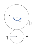
Figure 1: The left panel shows the net of a cone cut out from $T^{2}/\mathbb{Z}_{2}$ with the coordinates of $T^{2}/\mathbb{Z}_{2}$ $z$ and the cut edge $w$, whereas in the right panel, the cone cut out by $T^{2}/\mathbb{Z}_{2}$ whose coordinate is $z$ and a section of embedded quarter of $S^{2}$ with radius $r/\sqrt{3}$ whose coordinate is $z^{\prime}$ or $w$ are drawn.

Let us move on to the zero-mode wavefunctions on the resolution of $T^{2}/\mathbb{Z}_{2}$ orbifold through the above geometrical procedure. As discussed in Ref. [14], the zero-mode wavefunction of scalar field on $\mathbb{CP}^{1}\simeq S^{2}$ with $U(1)$ magnetic flux $M^{\prime}$ is described by

$$\phi^{j,|M^{\prime}|}_{S^{2}}(z^{\prime})={\cal N^{\prime}}^{j,|M^{\prime}|}\frac{f^{j,|M^{\prime}|}(z^{\prime})}{\left(1+|z^{\prime}|^{2}\right)^{|M^{\prime}|/2}},$$ (13)

where $f^{j,|M^{\prime}|}(z^{\prime})$ is the holomorphic function in the coordinate of $\mathbb{CP}^{1}$ $z^{\prime}$ with the zero-mode index $j$ determined by the flux $|M^{\prime}|$ and ${\cal N^{\prime}}^{j,|M^{\prime}|}$ is the normalization factor. The reason why we take the same index $j$ appearing in $T^{2}/\mathbb{Z}_{2}$ wavefunctions is to smoothly connect $S^{2}$ and $T^{2}/\mathbb{Z}_{2}$ wavefunctions in the blow-down limit $r\rightarrow 0$. The zero-mode wavefunction of fermion is also the same functional form but the meaning of $M^{\prime}$ is modified to the effective magnetic flux due to the curvature of $S^{2}$. The $S^{2}$ coordinate $z^{\prime}$ is related to the $T^{2}/\mathbb{Z}_{2}$ coordinate $z$ through another coordinate of $S^{2}$ $w$, which is written by $w=\frac{r}{2}\sqrt{3}z^{\prime}=\frac{r}{2}e^{i\varphi}$ at $\theta=\theta_{0}$ while $z=re^{i\varphi/2}$ at the same point as shown in FIG. 1, where $z^{\prime}=\tan\frac{\theta}{2}e^{i\varphi}$ in the setup of FIG. 1.

Thus, in order for the $T^{2}/\mathbb{Z}_{2}$ wavefunction at $z=re^{i\varphi/2}$ smoothly to connect with the $S^{2}$ wavefunction at $z^{\prime}=\frac{1}{\sqrt{3}}e^{i\varphi}$, the following conditions must be satisfied

$$\phi_{T^{2}/\mathbb{Z}_{2}^{\pm}}^{j,|M|}(z)\biggl{|}_{z=re^{i\varphi/2}} = \phi^{j,|M^{\prime}|}_{S^{2}}(z^{\prime})\biggl{|}_{z^{\prime}=\frac{1}{\sqrt{3}}e^{i\varphi}},$$

$$\frac{d\phi_{T^{2}/\mathbb{Z}_{2}^{\pm}}^{j,|M|}(z)}{dz}\biggl{|}_{z=re^{i\varphi/2}} = \frac{1}{\frac{\sqrt{3}}{2}r}\frac{d\phi^{j,|M^{\prime}|}_{S^{2}}(z^{\prime})}{dz^{\prime}}\biggl{|}_{z^{\prime}=\frac{1}{\sqrt{3}}e^{i\varphi}}.$$ (14)

Here, we take the Ansatz in Ref. [13] that the holomorphic part of $T^{2}/\mathbb{Z}_{2}$ wavefunction (12), denoted by the following $h^{j,|M|}(z)$

$$h^{j,|M|}(z)=\left\{\begin{array}[]{c}g^{j,|M|}(z),\qquad(j=0,|M|/2,\ \mathbb{Z}_{2}\text{-even})\\ \frac{g^{j,|M|}(z)+g^{j,|M|-j}(z)}{\sqrt{2}},\qquad(0<j<|M|/2,\ \mathbb{Z}_{2}\text{-even})\\ \frac{g^{j,|M|}(z)+g^{j,|M|-j}(z)}{\sqrt{2}},\qquad(0<j<|M|/2,\ \mathbb{Z}_{2}\text{-odd})\end{array}\right.$$ (18)

with

$$g^{j,|M|}(z)\equiv e^{\frac{\pi|M|}{2{\rm Im}\tau}z^{2}}\vartheta\begin{bmatrix}\frac{j}{|M|}\\ 0\end{bmatrix}(|M|z,|M|\tau),$$ (19)

is unchanged after the blow-up. Under the coordinate transformation $z\rightarrow w$, the transformation of the derivative of $S^{2}$ holomorphic function $f^{j,|M^{\prime}|}$ is provided by

$$\frac{df^{j,|M^{\prime}|}(z)}{dz}\biggl{|}_{z=re^{i\varphi/2}}=\frac{df^{j,|M^{\prime}|}(w)}{dw}\biggl{|}_{z=\frac{r}{2}e^{i\varphi}}=\frac{1}{\frac{\sqrt{3}}{2}r}\frac{df^{j,|M^{\prime}|}(\frac{\sqrt{3}}{2}rz^{\prime})}{dz^{\prime}}\biggl{|}_{z^{\prime}=\frac{1}{\sqrt{3}}e^{i\varphi}}.$$ (20)

Then, from the non-holomorphic parts in the condition for the continuous connection (14), the following conditions are obtained

$$\frac{{\cal N}^{j,|M|}_{1}}{{\cal N^{\prime}}^{j,|M^{\prime}|}_{1}}=\left(\frac{\sqrt{3}}{2}\right)^{|M^{\prime}|}e^{\frac{|M^{\prime}|}{4}},\qquad\frac{|M^{\prime}|}{4}=\frac{\pi r^{2}}{2{\rm Im}\tau}|M|.$$ (21)

The former condition shows the relation between the normalization factor of the $T^{2}/\mathbb{Z}_{2}$ part ${\cal N}^{j,|M|}_{1}$ and that of the $S^{2}$ part ${\cal N^{\prime}}^{j,|M^{\prime}|}_{1}$, and the latter condition shows that the embedded effective flux equals to the cut-out effective flux . In other words, the amount of the effective flux quanta is unchanged through the blow-up. On the other hand, from the Ansatz and the coordinate transformation (20), the $S^{2}$ holomorphic function $f^{j,|M^{\prime}|}(z^{\prime})$ is determined by using Eq. (19) as the following

$$f^{j,|M^{\prime}|}(z^{\prime})=\left\{\begin{array}[]{c}g^{j,|M|}\left(\frac{\sqrt{3}}{2}rz^{\prime}\right),\qquad(j=0,|M|/2,\ \mathbb{Z}_{2}\text{-even})\\ \sqrt{2}g^{j,|M|}\left(\frac{\sqrt{3}}{2}rz^{\prime}\right),\qquad(0<j<|M|/2,\ \mathbb{Z}_{2}\text{-even})\\ 0,\qquad(0<j<|M|/2,\ \mathbb{Z}_{2}\text{-odd})\end{array}\right.,$$ (25)

where we use the facts that $\vartheta^{|M|-j,M}(z)=\vartheta^{j,|M|}(ze^{i\pi})$ and the argument of $z^{\prime}$ is twice as much as that of $z$. Recall that $M^{\prime}$ is related to $M$ through Eq. (21). The above holomorphic functions show that only $\mathbb{Z}_{2}$-even mode is uplifted to $S^{2}$ and they are consistent with the fact that the $\mathbb{Z}_{2}$-odd mode vanishes at the fixed point $z_{I}=0$ in the blow-down limit $r\rightarrow 0$. Note that the same applies to the case of the blow-up of the singularities at $z_{I}=1/2,\tau/2$ because of $g^{j,|M|}(-z_{I})=g^{j,|M|}(z_{I})$, while in the case of the blow-up of the singularity at $z_{I}=(\tau+1)/2$, only $\mathbb{Z}_{2}$-even (-odd) mode is uplifted to $S^{2}$ when the flux $M$ is even (odd) because of $g^{j,|M|}(-z_{I})=e^{i\pi|M|}g^{j,|M|}(z_{I})$.

As a result, the zero-mode wavefunctions after the blow-up of the singularity at $z_{I}=0$ are described by

$$\phi^{j,|M|}_{\rm up}=\left\{\begin{array}[]{c}\phi^{j,|M^{\prime}|}_{S^{2}}=\cfrac{{\cal N^{\prime}}^{j,|M^{\prime}|}_{1}}{\left(1+|z^{\prime}|^{2}\right)^{\frac{|M^{\prime}|}{2}}}f^{j,|M^{\prime}|}(z^{\prime})\qquad(|z^{\prime}|\leq\frac{1}{\sqrt{3}})\\ \phi^{j,|M|}_{T^{2}/\mathbb{Z}_{2}}={\cal N}^{j,|M|}_{1}e^{-\frac{\pi|M||z|^{2}}{2{\rm Im}\tau}}h^{j,|M|}(z)\qquad(|z|\geq r)\end{array}\right.,$$ (28)

with Eq. (21), where the $S^{2}$ holomorphic function $f^{j,|M^{\prime}|}(z^{\prime})$ and the $T^{2}/\mathbb{Z}_{2}$ holomorphic function $h^{j,|M|}(z)$ are shown in Eq. (25) and Eq. (18), respectively. Note that the fermionic zero-mode wavefunctions $\psi^{j,|M|}_{\rm up}$ are also the same functional forms, but the meaning of $M^{\prime}$ is modified to the effective magnetic flux. The normalization factors are calculated by the wavefunctions (28),

$$\left|{\cal N}^{j,|M|}_{1}\right|\simeq\left\{\begin{array}[]{c}\left|{\cal N}^{j,|M|}\right|,\qquad(j=0,|M|/2,\ \mathbb{Z}_{2}\text{-even})\\ \left|{\cal N}^{j,|M|}\right|\left(1-\frac{1}{2\pi}\left(\frac{\pi r^{2}}{2}\right)^{2}\left|\left[\phi^{j,|M|}_{T^{2}/\mathbb{Z}_{2}^{-}}\right]^{\prime}\left(0\right)\right|^{2}\right),\qquad(0<j<|M|/2,\ \mathbb{Z}_{2}\text{-even})\\ \left|{\cal N}^{j,|M|}\right|\left(1+\frac{1}{2\pi}\left(\frac{\pi r^{2}}{2}\right)^{2}\left|\left[\phi^{j,|M|}_{T^{2}/\mathbb{Z}_{2}^{-}}\right]^{\prime}\left(0\right)\right|^{2}\right),\qquad(0<j<|M|/2,\ \mathbb{Z}_{2}\text{-odd})\end{array}\right.,$$ (32)

where ${\cal N}^{j,|M|}=(2|M|{\rm Im}(\tau)/{\cal A}^{2})^{1/4}$ is the normalization factor on $T^{2}/\mathbb{Z}_{2}$ before the blow-up and $\phi^{j,|M|}_{T^{2}/\mathbb{Z}_{2}^{-}}$ is the $\mathbb{Z}_{2}$-odd wavefunction on $T^{2}/\mathbb{Z}_{2}$ before the blow-up. Note that $\left[\phi^{j,|M|}_{T^{2}/\mathbb{Z}_{2}^{+}}\right]^{\prime}\left(0\right)\equiv\frac{d\phi^{j,|M|}_{T^{2}/\mathbb{Z}_{2}^{+}}}{dz}\Biggl{|}_{z=0}=0$. Furthermore, the normalization factor of the $S^{2}$ part is obtained from the normalization relation (21). Note that the blow-up radius should be smaller than $1/2$ to ensure our analysis, otherwise the blow-up region exceeds the bulk region

So far, we have focused on $U(1)$ magnetic flux background, but it is easy to extend the case with the following $U(N)$ magnetic flux,

$$F_{z\bar{z}}=\frac{i\pi}{{\rm Im}\tau}\begin{pmatrix}M_{a}\mathbb{I}_{N_{a}}&\ \\ \ &M_{b}\mathbb{I}_{N_{b}}\end{pmatrix},$$ (33)

where $N_{a}+N_{b}=N$ and $\mathbb{I}_{N_{a,b}}$ denotes the $(N_{a,b}\times N_{a,b})$ identity matrix, which breaks the $U(N)$ gauge symmetry to $U(N_{a})\times U(N_{b})$. Under this gauge background, the chiral zero-mode wavefunctions with the representation $(N_{a},\bar{N_{b}})$ are given by the same functional forms with the $U(1)$ gauge background but the flux $M$ is written by $M=M_{a}-M_{b}$.

3 The model

In this section, we study a model containing three generations of quarks on the resolutions of the toroidal orbifold background, where the orbifold fixed points are blown up.

As an illustrating model, we use the flavor model in Ref. [5]. This model is ten-dimensional $U(8)$ supersymmetric Yang-Mills theory compactified on $T^{6}/(\mathbb{Z}_{2}\times\mathbb{Z}_{2})$. The six-dimensional $T^{6}$ is written by a product of three $T^{2}$’s, i.e. $T^{6}=T^{2}_{1}\times T^{2}_{2}\times T^{2}_{3}$, where we denote the $i$-th complex coordinate on $T^{2}_{i}$ by $z_{i}$. There are three adjoint matter fields $\Phi_{i}$ ($i=1,2,3$) in the terminology of four-dimensional supersymmetric theory, where $\Phi_{i}$ have the vector index on $z_{i}$. These chiral matter fields correspond to the left-handed and right-handed fermions and Higgs fields. For example, the left-handed (right-handed) quarks and leptons are originated from $\Phi_{1}$ ($\Phi_{2}$), while the up and down Higgs fields correspond to $\Phi_{3}$. In the model of Ref. [5], magnetic fluxes of $U(8)$ are introduced in the extra dimensions such that three generations of quarks and leptons are realized and four-dimensional ${\cal N}=1$ supersymmetry remains. Zero-mode wavefunctions of each $\Phi_{i}$ are written by products of three wavefunctions on $z_{j}$, $\Phi_{i}=\prod_{j=1}^{3}\phi_{i(j)}(z_{j})$. The left-handed and right-handed quarks and leptons have three zero-modes on one of $z_{j}$, say $z_{1}$, while their zero-modes are single functions on the other four-dimensional space. That is, the flavor structure is determined by wavefunctions on $T^{2}_{1}$, while the other parts are relevant to only the overall factors of Yukawa couplings. Thus, here we concentrate on only the first two-dimensional part, $T^{2}_{1}/\mathbb{Z}_{2}$. Then, we use the six-dimensional model on $T^{2}/\mathbb{Z}_{2}$, which leads to the same mass ratios and mixing angles as the model in Ref. [5] in order to illustrate blow-up effects on mass matrices. In particular, we focus on the quark sector.

In the six-dimensional supersymmetric theory, $\Phi_{1}$ corresponds to the extra dimensional direction of the vector multiplet, while $\Phi_{2,3}$ are hypermultiplets. We set the magnetic fluxes and $\mathbb{Z}_{2}$ parity such that the magnetic flux $M=-5$ ($-7$) appears in the zero-mode equation for the left-handed (right-handed) quarks and they are $\mathbb{Z}_{2}$ even (odd), while the magnetic flux $M=12$ appears in the zero-mode equation for the up and down Higgs fields. Then, it turns out that quarks have three degenerate zero-modes, whereas there exist five degenerate zero-modes for the up and down Higgs sectors. TABLE 2 shows these behavior.

	Left-handed quarks	Right-handed quarks	Higgs
$M$  ($\mathbb{Z}_{2}$ parity)	$-5$  (even)	$-7$  (odd)	12  (odd)

Table 2: Magnetic fluxes for left- and right-handed quarks and Higgs sectors.

Each wavefunction is described as in Eq. (28), where the label $j$ is replaced by $I\ (0\leq I\leq 2)$, $J+1\ (0\leq J\leq 2)$, and $K+1\ (0\leq K\leq 4)$ for the left-handed quarks, the right-handed quarks, and the Higgs fields, respectively. Then, Yukawa couplings of the quark sector are written by

$$Y_{IJK}H_{K}Q_{LI}Q_{RJ}=(Y_{IJ0}H_{0}+Y_{IJ1}H_{1}+Y_{IJ2}H_{2}+Y_{IJ3}H_{3}+Y_{IJ4}H_{4})Q_{LI}Q_{RJ},$$ (34)

where $Q_{LI}$, $Q_{RJ}$, and $H_{K}$ are the four-dimensional left-handed and right-handed quarks and the Higgs fields, respectively and $Y_{IJK}$ is calculated as follows:

$$Y_{IJK} = \int_{T^{2}/\mathbb{Z}_{2}}dzd\bar{z}\ \phi^{I,5}_{T^{2}/\mathbb{Z}_{2}^{+}}(z)\phi^{J+1,7}_{T^{2}/\mathbb{Z}_{2}^{-}}(z)\left(\phi^{K+1,12}_{T^{2}/\mathbb{Z}_{2}^{-}}(z)\right)^{\ast}$$ (35)

$$- \sum_{z_{I}}\int_{\left|z-z_{I}\right|\leq r}dzd\bar{z}\ \phi^{I,5}_{T^{2}/\mathbb{Z}_{2}^{+}}(z)\phi^{J+1,7}_{T^{2}/\mathbb{Z}_{2}^{-}}(z)\left(\phi^{K+1,12}_{T^{2}/\mathbb{Z}_{2}^{-}}(z)\right)^{\ast},$$

where the first term is the whole $T^{2}/\mathbb{Z}_{2}$ term and the second term is the cut-out term from $T^{2}/\mathbb{Z}_{2}$. In addition, the terms on the $S^{2}$ regions after the blow-up of the singularities are needed originally but all of them become zero because the wavefunctions of the right-handed quarks and Higgs fields vanish on the $S^{2}$ regions after the blow-up of the singularities at $z_{I}=0,1/2,\tau/2$ and the wavefunctions of the left-handed quarks and Higgs fields vanish on the $S^{2}$ region after the blow-up of the singularities at $z_{I}=(\tau+1)/2$. The explicit form of the first term in Eq. (35) is shown in Ref. [2, 5], and the second term is calculated

$$\int_{\left|z-z_{i}\right|\leq r}dzd\bar{z}\ \phi^{I,5}_{T^{2}/\mathbb{Z}_{2}^{+}}(z)\phi^{J+1,7}_{T^{2}/\mathbb{Z}_{2}^{-}}(z)\left(\phi^{K+1,12}_{T^{2}/\mathbb{Z}_{2}^{-}}(z)\right)^{\ast}$$ (36)

$$\simeq \frac{1}{2\pi}\left(\frac{\pi r^{2}}{2}\right)^{2}\left(\phi^{I,5}_{T^{2}/\mathbb{Z}_{2}^{+}}\phi^{J+1,7}_{T^{2}/\mathbb{Z}_{2}^{-}}\right)^{\prime}(z_{I})\left(\phi^{\prime k,M}_{T^{2}/\mathbb{Z}_{2}^{-}}(z_{I})\right)^{\ast},$$

whose explicit form is shown in Appendix A. In the following analysis, we focus on two cases: blowing up all the fixed points, each with the same blow-up radius in Section 3.1 and different blow-up radii in Section 3.2.

3.1 Model 1

Here, we study the model, where the blow-up radii of the four fixed points are the same. We chose $\cos(\pi/6)H_{4}-\sin(\pi/6)H_{3}$ and $\sin(\pi/6)H_{4}+\cos(\pi/6)H_{3}$ as the directions of the vacuum expectation values (VEVs) for the up- and down-type Higgs fields, respectively. The reason to consider two pairs of Higgs doublets is that one can not realize the realistic masses and mixing angles of the quark sector with one pair of Higgs doublets. The Yukawa matrices $Y_{K=3}$ and $Y_{K=4}$ are approximated as

$$\begin{split}Y_{K=3}&=\frac{a}{\sqrt{2}}\begin{pmatrix}\sqrt{2}\eta_{10000}&\sqrt{2}\eta_{6400}&-\sqrt{2}\eta_{400}\\ \eta_{4624}&-\eta_{1024}&\eta_{64}\\ -\eta_{1936}&\eta_{16}&-\eta_{4096}\end{pmatrix}-\pi^{3}r^{4}\frac{a}{\sqrt{2}}\begin{pmatrix}8\sqrt{2}\eta_{1040}&96\sqrt{2}\eta_{800}&-8\sqrt{2}\eta_{680}\\ 176\eta_{704}&16\eta_{464}&128\eta_{344}\\ 48\eta_{536}&128\eta_{296}&16\eta_{176}\end{pmatrix},\\ Y_{K=4}&=\frac{a}{\sqrt{2}}\begin{pmatrix}\sqrt{2}\eta_{21025}&-\sqrt{2}\eta_{625}&\sqrt{2}\eta_{7225}\\ \eta_{529}&\eta_{5329}&-\eta_{169}\\ \eta_{121}&\eta_{121}&\eta_{1}\end{pmatrix}-\pi^{3}r^{4}\frac{a}{\sqrt{2}}\begin{pmatrix}87\sqrt{2}\eta_{935}&0&63\sqrt{2}\eta_{575}\\ 28\eta_{594}&126\eta_{359}&0\\ 126\eta_{431}&28\eta_{191}&98\eta_{71}\end{pmatrix},\end{split}$$ (37)

where the overall factor $a=\frac{\left|{\cal N}^{I,5}_{1}{\cal N}^{J+1,7}_{1}{\cal N}^{K+1,12}_{1}\right|}{\left|{\cal N}^{K+1,12}\right|^{2}}$ and we assume $\pi\tau=5.7i$ and $\eta_{n}\equiv e^{-5.7n/420}$, originating from the approximation of the Jacobi theta function. (For more details on the calculation, see, Appendix A.) By employing the above Yukawa couplings, we calculate the mass ratios of the up/charm quark to the top quark and the down/strange quark to the bottom quark, and Cabibbo-Kobayashi-Maskawa (CKM) matrix. We show the $r$-dependence of them in FIGs. 2 and 3, where the maximum of $r$ is set to be $0.25$ since we use the same $r$ for all the fixed points and the distance to the nearest fixed points is $0.5$.

From FIGs. 2 and 3, it is found that the blow-up of the orbifold singularities significantly affects the quark masses and the CKM matrices. Table 3 shows the mass ratios and the CKM matrix at $r\approx 0.24\ (\pi^{3}r^{4}=0.105)$, and the table also shows the results in the case of $r=0$, that is the $T^{2}/\mathbb{Z}_{2}$ orbifold limit, and the experimental data for magnitudes of CKM elements [17] and quark masses evaluated at the so-called GUT scale $2.0\times 10^{16}\,{\rm GeV}$ [16]. Thus, we find that the blow-up of the orbifold singularities makes the values approach the observed values up to $O(1)$.

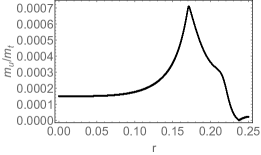
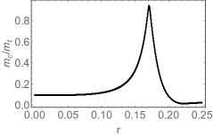
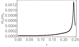
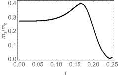
Figure 2: The blow-up radius ($r$)-dependence of the mass ratios of the up quark to the top quark $m_{u}/m_{t}$, the charm quark to the top quark $m_{c}/m_{t}$, the down quark to the bottom quark $m_{d}/m_{b}$, and the strange quark to the bottom quark $m_{s}/m_{b}$.

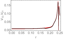
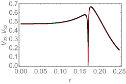
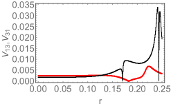
Figure 3: The blow-up radius ($r$)-dependence of the CKM mixing angles $V_{12}(V_{21})$, $V_{23}(V_{32})$, and $V_{13}(V_{31})$, as shown in the red (black) lines.

	Pure $T^{2}/\mathbb{Z}_{2}$ ($r=0$)	Blow-ups of $T^{2}/\mathbb{Z}_{2}$ ($r\approx 0.24$)	Observed values
$(m_{u},m_{c},m_{t})/m_{t}$	$(1.5\times 10^{-4},9.6\times 10^{-2},1)$	$(1.2\times 10^{-5},2.3\times 10^{-2},1)$	$(6.5\times 10^{-6},3.2\times 10^{-3},1)$
$(m_{d},m_{s},m_{b})/m_{b}$	$(2.5\times 10^{-5},2.7\times 10^{-1},1)$	$(9.7\times 10^{-4},6.3\times 10^{-3},1)$	$(1.1\times 10^{-3},2.2\times 10^{-2},1)$
$|V_{CKM}|$	$\begin{pmatrix}1.0&0.0082&0.0022\\ 0.0084&0.88&0.47\\ 0.0017&0.47&0.88\end{pmatrix}$	$\begin{pmatrix}0.99&0.17&0.0043\\ 0.17&0.96&0.22\\ 0.034&0.22&0.98\end{pmatrix}$	$\begin{pmatrix}0.97&0.22&0.0037\\ 0.22&0.97&0.042\\ 0.0090&0.041&1.0\end{pmatrix}$

Table 3: The mass ratios and CKM matrices for the blow-up radius $r=0$ (the pure $T^{2}/\mathbb{Z}_{2}$ orbifold), $r\approx 0.24$, and the observed values, where we use the GUT scale running masses [16].

3.2 Model 2

So far, we have taken into account the blow-up of all the fixed points, each with the same blow-up radius, but there is no reason to take the same values of blow-up radii which can be determined by the dynamics of blow-up modes, i.e. the blow-up moduli stabilization.

In this section, we examine the case where the blow-up radius at $z_{I}=\tau/2$ fixed point $r_{\tau/2}$ is different from the others, namely $r=r_{0}=r_{1/2}=r_{(\tau+1)/2}$, where $r_{0}$, $r_{1/2}$, $r_{\tau/2}$ $r_{(\tau+1)/2}$ denote the blow-up radii at the fixed points $z_{I}=0,1/2,\tau/2,(\tau+1)/2$, respectively. To simplify our analysis, we focus on the model with one pair of Higgs doublets, where the up- and down-type Higgs fields are identified with $H_{u}=H_{4}$ and $H_{d}=H_{3}$. The Yukawa coupling $Y_{IJK}$ in Eq. (35) is calculated by using the formulae in Appendix A. In a way similar to the previous section, we draw the mass ratios and magnitudes of CKM elements as a function of blow-up radius $r$ in FIGs. 4 and 5, in which we assume

$$\tau=1.8i,\qquad r_{\tau/2}=2.6\times r.$$ (38)

It indicates that the maximum value of $r$ is $0.139$, otherwise two blow-up regions associated with the fixed points $z=\tau/2$ and $z=(\tau+1)/2$ overlap with each other.

Table 4 shows the predictions of the mass ratios and the CKM mixing angles for both the magnetized orbifold model ($r=0$) and the magnetized blow-up model ($r=0.12$). It turns out that the rank of down-type quark mass matrix is 2 in the toroidal orbifold model, but blowing up the fixed points leads to the rank 3 mass matrix and more realistic flavor structure.

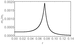
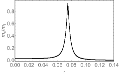
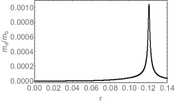
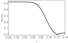
Figure 4: The blow-up radius ($r$)-dependence of the mass ratios of the up quark to the top quark $m_{u}/m_{t}$, the charm quark to the top quark $m_{c}/m_{t}$, the down quark to the bottom quark $m_{d}/m_{b}$, and the strange quark to the bottom quark $m_{s}/m_{b}$.

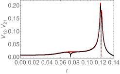
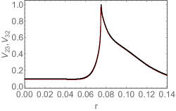
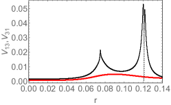
Figure 5: The blow-up radius ($r$)-dependence of the CKM mixing angles $V_{12}(V_{21})$, $V_{23}(V_{32})$, and $V_{13}(V_{31})$, as shown in the red (black) lines.

	Pure $T^{2}/\mathbb{Z}_{2}$ ($r=0$)	Blow-ups of $T^{2}/\mathbb{Z}_{2}$ ($r=0.12$)	Observed values
$(m_{u},m_{c},m_{t})/m_{t}$	$(2.2\times 10^{-4},2.7\times 10^{-2},1)$	$(5.3\times 10^{-5},5.2\times 10^{-3},1)$	$(6.5\times 10^{-6},3.2\times 10^{-3},1)$
$(m_{d},m_{s},m_{b})/m_{b}$	$(0,5.2\times 10^{-1},1)$	$(7.6\times 10^{-4},3.9\times 10^{-3},1)$	$(1.1\times 10^{-3},2.2\times 10^{-2},1)$
$|V_{CKM}|$	$\begin{pmatrix}1.0&0.0080&0.00077\\ 0.0084&1.0&0.096\\ 0.0015&0.0096&1.0\end{pmatrix}$	$\begin{pmatrix}0.98&0.21&0.0032\\ 0.20&0.94&0.27\\ 0.053&0.26&0.96\end{pmatrix}$	$\begin{pmatrix}0.97&0.22&0.0037\\ 0.22&0.97&0.042\\ 0.0090&0.041&1.0\end{pmatrix}$

Table 4: The mass ratios and CKM matrices for the blow-up radius $r=0$ (the pure $T^{2}/\mathbb{Z}_{2}$ orbifold), $r=0.12$, and the observed values, where we use the GUT scale running masses [16].

4 Conclusions

We have examined the flavor structure of magnetized $T^{2}/\mathbb{Z}_{2}$ blow-up models, where the orbifold fixed points are replaced by a part of sphere proposed by the method in Ref. [13]. The flavor structure as well as the selection rules of Yukawa couplings among chiral zero-modes are different from the toroidal orbifold results, due to the blowing up the orbifold singularities as demonstrated in a concrete model in Section 3. Interestingly, the elements of the CKM matrix and mass hierarchy of the quark sector are well consistent with the observed data at certain values of the blow-up radii, rather than the toroidal orbifold result. Furthermore, such a realistic setup can be realized by a few number of parameters, although in toroidal orbifold case, several pairs of Higgs doublets are required to explain the observed flavor structure and mass hierarchy of the quark sector.

In this paper, we have assumed that the blow-up modes determining the blow-up radii are considered just the parameter, but it should be taken as a dynamical degree of freedom. It is interesting to discuss the dynamics of the blow-up modes such that their vacuum expectation values lead to the observed data. We have focused on the simplest $T^{2}/\mathbb{Z}_{2}$ case, but our analysis can be generalized to resolutions of $T^{2}/\mathbb{Z}_{N}$ orbifolds . Another possible generalization of our work is to apply our method to the resolutions of higher dimensional toroidal orbifolds . We hope to report on these subjects in the future.

Appendix A Correction terms of Yukawa coupling

Here, we show the explicit calculation of Eq. (36) at each singularity as follows:

$$\int_{\left|z\right|\leq r}dzd\bar{z}\ \phi^{I,5}_{T^{2}/\mathbb{Z}_{2}^{+}}(z)\phi^{J+1,7}_{T^{2}/\mathbb{Z}_{2}^{-}}(z)\left(\phi^{K+1,12}_{T^{2}/\mathbb{Z}_{2}^{-}}(z)\right)^{\ast}$$

$$\simeq\frac{1}{2\pi}\left(\frac{\pi r^{2}}{2}\right)^{2}\phi^{I,5}_{T^{2}/\mathbb{Z}_{2}^{+}}(0)\phi^{\prime J+1,7}_{T^{2}/\mathbb{Z}_{2}^{-}}(0)\left(\phi^{\prime k,M}_{T^{2}/\mathbb{Z}_{2}^{-}}(0)\right)^{\ast}$$

$$=\sqrt{2}\pi^{3}r^{4}a\sum_{l,m,n}\left(J+1+7m\right)\left(K+1+12n\right)e^{-\pi{\rm Im}\tau\left[5\left(\frac{I}{5}+l\right)^{2}+7\left(\frac{J+1}{7}+m\right)^{2}+12\left(\frac{K+1}{12}+n\right)^{2}\right]}$$

$$\simeq\sqrt{2}\pi^{3}r^{4}a\left(J+1\right)\left(K+1\right)e^{-\pi{\rm Im}\tau\frac{84I^{2}+60\left(J+1\right)^{2}+35\left(K+1\right)^{2}}{420}}$$

$$=\sqrt{2}\pi^{3}r^{4}a\left(J+1\right)\left(K+1\right)\eta_{84I^{2}+60\left(J+1\right)^{2}+35\left(K+1\right)^{2}},$$ (39)

$$\int_{\left|z-\frac{1}{2}\right|\leq r}dzd\bar{z}\ \phi^{I,5}_{T^{2}/\mathbb{Z}_{2}^{+}}(z)\phi^{J+1,7}_{T^{2}/\mathbb{Z}_{2}^{-}}(z)\left(\phi^{K+1,12}_{T^{2}/\mathbb{Z}_{2}^{-}}(z)\right)^{\ast}$$

$$\simeq\frac{1}{2\pi}\left(\frac{\pi r^{2}}{2}\right)^{2}\phi^{I,5}_{T^{2}/\mathbb{Z}_{2}^{+}}(\frac{1}{2})\phi^{\prime J+1,7}_{T^{2}/\mathbb{Z}_{2}^{-}}(\frac{1}{2})\left(\phi^{\prime k,M}_{T^{2}/\mathbb{Z}_{2}^{-}}(\frac{1}{2})\right)^{\ast}$$

$$=\sqrt{2}\pi^{3}r^{4}a\sum_{l,m,n}\left(J+1+7m\right)\left(K+1+12n\right)$$

$$\times e^{-\pi{\rm Im}\tau\left[5\left(\frac{I}{5}+l\right)^{2}+7\left(\frac{J+1}{7}+m\right)^{2}+12\left(\frac{K+1}{12}+n\right)^{2}\right]}e^{\pi i\left[\left(I+5l\right)+\left(J+1+7m\right)-\left(K+1+12n\right)\right]}$$

$$\simeq\sqrt{2}\pi^{3}r^{4}a\left(J+1\right)\left(K+1\right)e^{-\pi{\rm Im}\tau\frac{84I^{2}+60\left(J+1\right)^{2}+35\left(K+1\right)^{2}}{420}}e^{\pi i\left(I+J-K\right)}$$

$$=\sqrt{2}\pi^{3}r^{4}a\left(J+1\right)\left(K+1\right)\eta_{84I^{2}+60\left(J+1\right)^{2}+35\left(K+1\right)^{2}}e^{\pi i\left(I+J-K\right)},$$ (40)

$$\int_{\left|z-\frac{\tau}{2}\right|\leq r}dzd\bar{z}\ \phi^{I,5}_{T^{2}/\mathbb{Z}_{2}^{+}}(z)\phi^{J+1,7}_{T^{2}/\mathbb{Z}_{2}^{-}}(z)\left(\phi^{K+1,12}_{T^{2}/\mathbb{Z}_{2}^{-}}(z)\right)^{\ast}$$

$$\simeq\frac{1}{2\pi}\left(\frac{\pi r^{2}}{2}\right)^{2}\phi^{I,5}_{T^{2}/\mathbb{Z}_{2}^{+}}(\frac{\tau}{2})\phi^{\prime J+1,7}_{T^{2}/\mathbb{Z}_{2}^{-}}(\frac{\tau}{2})\left(\phi^{\prime k,M}_{T^{2}/\mathbb{Z}_{2}^{-}}(\frac{\tau}{2})\right)^{\ast}$$

$$=\sqrt{2}\pi^{3}r^{4}a\sum_{l,m,n}\left(J+1+7m\right)\left(K+1+12n\right)e^{-\pi{\rm Im}\tau\left[5\left(\frac{I}{5}+l+\frac{1}{2}\right)^{2}+7\left(\frac{J+1}{7}+m+\frac{1}{2}\right)^{2}+12\left(\frac{K+1}{12}+n+\frac{1}{2}\right)^{2}\right]}$$

$$\simeq\sqrt{2}\pi^{3}r_{3}^{4}a\left(7-\left(J+1\right)\right)\left(12-\left(K+1\right)\right)e^{-\pi{\rm Im}\tau\frac{2520-84I\left(5-I\right)-60\left(J+1\right)\left(7-\left(J+1\right)\right)-35\left(K+1\right)\left(12-\left(K+1\right)\right)}{420}}$$

$$=\sqrt{2}\pi^{3}r^{4}a\left(7-\left(J+1\right)\right)\left(12-\left(K+1\right)\right)\eta_{2520-84I\left(5-I\right)-60\left(J+1\right)\left(7-\left(J+1\right)\right)-35\left(K+1\right)\left(12-\left(K+1\right)\right)},$$ (41)

$$\int_{\left|z-\frac{\tau+1}{2}\right|\leq r}dzd\bar{z}\ \phi^{I,5}_{T^{2}/\mathbb{Z}_{2}^{+}}(z)\phi^{J+1,7}_{T^{2}/\mathbb{Z}_{2}^{-}}(z)\left(\phi^{K+1,12}_{T^{2}/\mathbb{Z}_{2}^{-}}(z)\right)^{\ast}$$

$$\simeq\frac{1}{2\pi}\left(\frac{\pi r^{2}}{2}\right)^{2}\phi^{\prime I,5}_{T^{2}/\mathbb{Z}_{2}^{+}}(\frac{\tau+1}{2})\phi^{J+1,7}_{T^{2}/\mathbb{Z}_{2}^{-}}(\frac{\tau+1}{2})\left(\phi^{\prime k,M}_{T^{2}/\mathbb{Z}_{2}^{-}}(\frac{\tau+1}{2})\right)^{\ast}$$

$$=\sqrt{2}\pi^{3}r^{4}a\sum_{l,m,n}\left(I+5l\right)\left(K+1+12n\right)$$

$$\times e^{-\pi{\rm Im}\tau\left[5\left(\frac{I}{5}+l+\frac{1}{2}\right)^{2}+7\left(\frac{J+1}{7}+m+\frac{1}{2}\right)^{2}+12\left(\frac{K+1}{12}+n+\frac{1}{2}\right)^{2}\right]}e^{\pi i\left[\left(I+5l\right)+\left(J+1+7m\right)-\left(K+1+12n\right)\right]}$$

$$\simeq\sqrt{2}\pi^{3}r^{4}a\left(5-I\right)\left(12-\left(K+1\right)\right)e^{-\pi{\rm Im}\tau\frac{2520-84I\left(5-I\right)-60\left(J+1\right)\left(7-\left(J+1\right)\right)-35\left(K+1\right)\left(12-\left(K+1\right)\right)}{420}}e^{\pi i\left(I+J-K\right)}$$

$$=\sqrt{2}\pi^{3}r^{4}a\left(5-I\right)\left(12-\left(K+1\right)\right)\eta_{2520-84I\left(5-I\right)-60\left(J+1\right)\left(7-\left(J+1\right)\right)-35\left(K+1\right)\left(12-\left(K+1\right)\right)}e^{\pi i\left(I+J-K\right)},$$ (42)

where the overall factor $a=\frac{\left|{\cal N}^{I,5}_{1}{\cal N}^{J+1,7}_{1}{\cal N}^{K+1,12}_{1}\right|}{\left|{\cal N}^{K+1,12}\right|^{2}}$ and we asuume ${\rm Re}\tau=0$ and approximate the Jacobi theta function by $\eta_{n}\equiv e^{-n\pi{\rm Im}\tau/420}$. Note that we need to multiply $1/\sqrt{2}$ further if $I=0$.

References

- [1] H. Abe, T. Kobayashi and H. Ohki, JHEP 0809, 043 (2008) [arXiv:0806.4748 [hep-th]].
- [2] H. Abe, K. S. Choi, T. Kobayashi and H. Ohki, Nucl. Phys. B 814, 265 (2009) [arXiv:0812.3534[hep-th]].
- [3] D. Cremades, L. E. Ibanez and F. Marchesano, JHEP 0405, 079 (2004) [hep-th/0404229].
- [4] H. Abe, T. Kobayashi, H. Ohki, A. Oikawa and K. Sumita, Nucl. Phys. B 870, 30 (2013) [arXiv:1211.4317 [hep-ph]].
- [5] H. Abe, T. Kobayashi, K. Sumita and Y. Tatsuta, Phys. Rev. D 90, no. 10. 105006 (2014) [arXiv:1405.5012[hep-ph]].
- [6] Y. Fujimoto, T. Kobayashi, K. Nishiwaki, M. Sakamoto and Y. Tatsuta, Phys. Rev. D 94, no. 3, 035031 (2016) [arXiv:1605.00140 [hep-ph]].
- [7] T. Kobayashi, K. Nishiwaki and Y. Tatsuta, JHEP 1704, 080 (2017) [arXiv:1609.08608 [hep-th]].
- [8] L. J. Dixon, J. A. Harvey, C. Vafa and E. Witten, Nucl. Phys. B 261 (1985) 678.
- [9] L. J. Dixon, J. A. Harvey, C. Vafa and E. Witten, Nucl. Phys. B 274 (1986) 285.
- [10] S. Groot Nibbelink, M. Trapletti and M. Walter, JHEP 0703 (2007) 035 [hep-th/0701227].
- [11] P. Leung and H. Otsuka, Phys. Rev. D 99 (2019) no.12, 126011 [arXiv:1903.12144 [hep-th]].
- [12] T. Eguchi and A. J. Hanson, Phys. Lett. 74B (1978) 249.
- [13] T. Kobayashi, H. Otsuka and H. Uchida, JHEP 1908, 046 (2019) [arXiv:1904.02867 [hep-th]].
- [14] J. P. Conlon, A. Maharana and F. Quevedo, JHEP 0809, 104 (2009) [arXiv:0807.0789 [hep-th]].
- [15] T. Kobayashi, Y. Tatsuta and S. Uemura, Phys. Rev. D 93, no. 6, 065029 (2016) [arXiv:1511.09256 [hep-ph]].
- [16] Z. z. Xing, H. Zhang and S. Zhou, Phys. Rev. D 77, 113016 (2008) [arXiv:0712.1419[hep-ph]].
- [17] M. Tanabashi et al. [Particle Data Group], Phys. Rev. D 98 (2018) no.3, 030001.
- [18] T. H. Abe, Y. Fujimoto, T. Kobayashi, T. Miura, K. Nishiwaki and M. Sakamoto, JHEP 1401, 065 (2014) [arXiv:1309.4925 [hep-th]].
- [19] T. h. Abe, Y. Fujimoto, T. Kobayashi, T. Miura, K. Nishiwaki and M. Sakamoto, Nucl. Phys. B 890, 442 (2014) [arXiv:1409.5421 [hep-th]].
- [20] M. Headrick and T. Wiseman, Class. Quant. Grav. 22 (2005) 4931 [hep-th/0506129].
- [21] C. P. Burgess, J. P. Conlon, L. Y. Hung, C. H. Kom, A. Maharana and F. Quevedo, JHEP 0807 (2008) 073 [arXiv:0805.4037 [hep-th]].
- [22] A. Maharana, JHEP 1206 (2012) 002 [arXiv:1111.3047 [hep-th]].