Star density profiles of six old star clusters in the Large Magellanic Cloud

Abstract

We used resolved star counts from Hubble Space Telescope images to determine the center of gravity and the projected density profiles of 6 old globular clusters in the Large Magellanic Cloud (LMC), namely NGC 1466, NGC 1841, NGC 1898, NGC 2210, NGC 2257 and Hodge 11. For each system the LMC field contribution was properly taken into account by making use, when needed, of parallel HST observations. The derived values of the center of gravity may differ by several arcseconds (corresponding to more dal 1 pc at the distance of the LMC) from previous determinations. The cluster density profiles are all well fit by King models, with structural parameters that may differ from the literature ones by even factors of two. Similarly to what observed for Galactic globular clusters, the ratio between the effective and the core radius has been found to anti-correlate with the cluster dynamical age.

1 Introduction

Globular clusters (GCs) are the best example in nature of collisional stellar systems, where multiple and multifold gravitational interactions occur among the constituent stars, significantly altering the physical properties of the host with respect to its conditions at formation (see, e.g., Meylan, & Heggie, 1997). In this context, we are carrying on a long-term project aimed at the accurate characterization of the internal structure, kinematics and stellar content of GCs. In particular, we are using number counts (Lanzoni et al., 2007a, b, c, 2010; Miocchi et al., 2013), in place of the surface brightness distributions, and the radial velocities of individual stars (Lanzoni et al., 2013, 2018a, 2018b; Ferraro et al., 2018a; see also Baumgardt, & Hilker, 2018), instead of integrated-light spectroscopy, to determine the cluster gravitational centers and the structural and kinematical parameters. This is to avoid the so-called “shot-noise bias” that is known to affect luminosity-weighted quantities (as the surface brightness distribution and integrated-light spectra) when dealing with resolved stellar populations. The bias is due to the stochastic and sparse presence of luminous stars, which can significantly displace the surface brightness peak from the true location of the cluster gravitational center, and alter the shape of the surface brightness profile with respect to the true density distribution (see, e.g., Noyola, & Gebhardt 2006 for a discussion of methods adopted to correct for this problem in photometric studies, and see Dubath et al. 1997, Lützgendorf et al. 2011, and Lanzoni et al. 2013 for a discussion of this bias in the case of integrated-light spectroscopy). The bias does not occur if resolved stars are used, since every object has the same weight, independently of its luminosity (e.g. Calzetti et al., 1993; Lugger et al., 1995; Montegriffo et al., 1995). In spite of their advantages, techniques based on star counts have not been fully exploited in the literature yet, and the vast majority of GC structural parameters listed in largely used catalogs (e.g., Harris, 1996; Mackey & Gilmore, 2003, hereafter MG03; McLaughlin & van der Marel, 2005, hereafter Mv05) have been derived from surface brightness distributions. This is essentially because constructing complete samples of resolved stars in the highly crowded central regions of GCs is not an easy task. In fact, even Hubble Space Telescope (HST) catalogs obtained from observations not optimized to avoid strong saturation from the bright giants can be severely incomplete in the central regions of high-density clusters (see Ferraro et al., 1997; Raso et al., 2017). However, starting from studies dedicated to specific objects or very small sets of clusters (e.g. Ferraro et al., 1999, 2003; Dalessandro et al., 2008, 2013, 2015; Salinas et al., 2012; Saracino et al., 2015; Cadelano et al., 2017), the systematic determination of gravitational centers and surface density profiles from resolved stars counts is increasingly adopted (see, e.g., the study of a sample of 26 Galactic GCs discussed in Miocchi et al. 2013).

For a full physical characterization of these systems we are also making use of the observational properties of special classes of stellar objects, like the so-called “blue straggler stars” (BSSs; e.g., Ferraro et al., 2006, 2009, 2012; Dalessandro et al., 2013; Beccari et al., 2019). In fact, BSSs are significantly more massive than normal cluster stars (e.g., Shara et al. 1997; Fiorentino et al. 2014; Raso et al. 2019) and dynamical friction thus makes them progressively sinking toward the cluster center. Correspondingly, their central segregation relative to a reference (lighter) population (as horizontal branch, red giant branch, main sequence stars) progressively increases with time. This can be quantitatively measured from the shape of the BSS radial distribution (e.g. Ferraro et al., 2012), and through the $A^{+}$ parameter, which is defined as the area enclosed between the cumulative radial distribution of BSSs and that of the reference population (Alessandrini et al., 2016; see also Lanzoni et al., 2016 for a comparison between the two approaches). Recently, Ferraro et al. (2018b) measured the value of $A^{+}$ within one half-mass radius from the center of 48 Galactic GCs ($\sim 32\%$ of the entire Milky Way population) and found a strong correlation with the number of central relaxation times ($N_{\rm rel}$) suffered by each system since formation. This demonstrates that $A^{+}$ is a powerful empirical “dynamical clock”, able to efficiently measure the level of internal dynamical evolution suffered by stellar systems (i.e., their dynamical age).

We are now extending the same approach adopted in the Milky Way, to star clusters located in the Large Magellanic Cloud (LMC). This nearby galaxy hosts stellar systems covering a wide range of ages (from a few million, to several billion years), at odds with the Milky Way where mostly old ($t>10$ Gyr) GCs are found. It therefore offers a unique opportunity to explore the formation process of star clusters over cosmic time, making the characterization of their physical properties crucial. In addition, since the LMC tidal field differs from that of the Milky Way, the dynamical evolution of the hosted clusters could be different as well (see, e.g., Piatti et al., 2019 for a recent study of the effect of the Milky Way tidal field on GC properties). Ferraro et al. (2019) measured the $A^{+}$ parameter in five old LMC clusters, finding that they follow the same correlations with $N_{\rm rel}$ drawn by the Milky Way systems. Here we focus on the determination of the projected density profiles and structural parameters (from resolved star counts) of the same systems studied by Ferraro et al. (2019), plus an additional one (NGC 1898) where the strong contamination from LMC field stars prevented us from a safe selection of the BSS population and the determination of $A^{+}$.

The paper is organized as follows. In Section 2 we present the photometric database used and the adopted data reduction procedures. In Sections 3 and 4 we discuss the determination of the cluster gravitational center and projected density profiles from the observed resolved stars. Section 5 is devoted to present the fit to the observed density profiles through King (1966) models, and the derivation of the cluster structural parameters. In Section 6 we discuss the obtained results.

Table 1: Data set

Cluster	Camera	Filter	Exposure Time	Prop. ID
NGC 1466	ACS/WFC	F606W	$2\times 50$ s, $12\times 353$ s	14164
	ACS/WFC	F814W	$2\times 70$ s, $6\times 352$ s, $6\times 385$ s, $6\times 420$ s
parallel	ACS/WFC	F435W	$12\times 575$ s
	ACS/WFC	F606W	$1\times 50$ s, $3\times 566$ s
NGC 1841	ACS/WFC	F606W	$2\times 50$ s, $12\times 353$ s	14164
	ACS/WFC	F814W	$2\times 70$ s, $6\times 352$ s, $6\times 385$ s, $6\times 420$ s
parallel	ACS/WFC	F435W	$12\times 575$ s
	ACS/WFC	F606W	$1\times 50$ s, $3\times 566$ s
NGC 1898	ACS/WFC	F475W	$2\times 500$ s	12257
	ACS/WFC	F814W	$2\times 500$ s
	WFC3/UVIS	F336W	$2\times 1035$ s	13435
NGC 2210	ACS/WFC	F606W	$2\times 50$ s, $6\times 348$ s, $6\times 353$ s	14164
	ACS/WFC	F814W	$2\times 70$ s, $6\times 344$ s, $6\times 378$ s, $6\times 413$ s
	WFC3/UVIS	F336W	$4\times 700$ s, $4\times 715$ s, $4\times 729$ s, $4\times 730$ s
parallel	ACS/WFC	F435W	$4\times 550$ s, $8\times 565$ s
	ACS/WFC	F606W	$1\times 50$ s, $3\times 560$ s
NGC 2257	ACS/WFC	F606W	$2\times 50$ s, $3\times 364$ s, $2\times 525$ s, $6\times 353$ s	14164
	ACS/WFC	F814W	$2\times 70$ s, $3\times 390$ s, $2\times 450$ s, $6\times 363$ s, $6\times 400$ s
parallel	ACS/WFC	F435W	$12\times 575$ s
	ACS/WFC	F606W	$1\times 50$ s, $3\times 570$ s
Hodge 11	ACS/WFC	F606W	$2\times 50$ s, $6\times 345$ s, $6\times 370$ s	14164
	ACS/WFC	F814W	$2\times 70$ s, $6\times 345$ s, $6\times 377$ s, $6\times 410$ s
	WFC3/UVIS	F336W	$3\times 700$ s , $12\times 729$ s
parallel	ACS/WFC	F435W	$4\times 550$ s, $8\times 570$ s
	ACS/WFC	F606W	$1\times 50$ s, $3\times 570$ s

Note. — Details of the HST archive images used in the present study.

2 Photometric database and data reduction

The data used in this paper consist in a set of archive images acquired with the Wide Field Channel of the Advanced Camera for Survey (ACS/WFC) and the UVIS channel of the Wide Field Camera 3 (WFC3/UVIS) on board the HST (see Table 1). For five of the selected clusters, the data are part of GO 14164 (PI Sarajedini) and consist in ACS/WFC observations in the F606W ($V$) and F814W ($I$) filters performed in the direction of each system, complemented with parallel ACS/WFC images of nearby fields ($\sim 5\arcmin$ from the cluster centers) acquired through the F435W ($B_{435}$) and F606W filters. In the case of NGC 2210 and Hodge 11 we also made use of the WFC3/UVIS pointings in the F336W, acquired under the same program. For NGC 1898 the images have been obtained with the ACS/WFC in the F475W ($B$) and F814W filters (GO 12257, PI Girardi), and with the WFC3/UVIS in the F336W (GO 13435, PI Monelli). In general, different pointings dithered by several pixels have been performed in each band, thus allowing the filling of the inter-chip gaps, and an adequate subtraction of CCD defects, artifacts, and false detections.

The photometric analysis was performed independently on each image via the point-spread function (PSF) fitting method, by using DAOPHOT IV and following the “standard” approach already used in previous works (e.g., Dalessandro et al., 2018). Briefly, PSF models were derived for each image and detector by using some dozens of bright and isolated stars, and then applied to all the detected sources with flux peaks at least $3\sigma$ above the local background. A master list including stars detected in at least two images was then created. At the position of all the stars in the master-list, a fit was forced in each frame with DAOPHOT/ALLFRAME (Stetson, 1994). In the case of NGC 1898, NGC 2210 and Hodge 11, the master list of detected sources has been constructed on the F336W images, and then forced to the exposures acquired in the other filters. As quantitatively demonstrated in Raso et al. (2017), photometric analyses guided by short-wavelength filters allow the optimization of the source detection in the overcrowded central regions of old stellar populations, where cool giant stars easily saturate in the optical bands and specific procedures are needed to try and correct for their blooming effects (see, e.g., Anderson et al., 2008 for more details). For every star thus recovered, the multiple magnitude estimates obtained in each chip with the same filter were homogenized by using DAOMATCH and DAOMASTER, and their weighted mean and standard deviation were finally adopted as the star magnitude and photometric error.

The instrumental magnitudes have been calibrated onto the VEGAMAG photometric system by using the recipes and zero-points reported in the HST web-sites. The instrumental coordinates were first corrected for geometric distortions by using the most updated ACS/WFC Distortion Correction Tables (IDCTAB) provided in the dedicated web page of the Space Telescope Science Institute. Then, they were reported to the absolute coordinate system ($\alpha,\delta$) as defined by the World Coordinate System using the stars in common with the publicly available Gaia DR2 catalog. The resulting astrometric accuracy is typically $<0.1$ mas.

Figures 1–5 show the color-magnitude diagrams (CMDs) obtained from these data in the direction of all the program clusters. As apparent, the cluster pointings are deep enough to nicely trace all the evolutionary sequences, reaching $\sim 2$ magnitudes below the main sequence turn-off (MS-TO) level. The CMDs obtained from the parallel observations of NGC 1466 and NGC 1841 are very sparse, with just 53 and 61 stars above $V=23$, respectively (and thus they are not shown). Those obtained in the nearby fields of NGC 2210, NGC 2257 and Hodge11 are, instead, more populated (see right panels in Figures 2–4), indicating that these three systems are located in denser regions of the LMC. Indeed, the presence of LMC field stars is well visible also in the corresponding cluster CMDs, especially for NGC 2210 and Hodge11 (Figure 2 and 4), as a prominent extension of the cluster MS at magnitudes brighter than the MS-TO point. In Figure 5 we show the CMD of NGC 1898, plotting separately the stars measured within $20\arcsec$ (illustrating the distribution of the cluster population; left panel), and those beyond $80\arcsec$ from the center, which are dominated by the LMC field population (right panel).

Figure 1: Color-magnitude diagrams of NGC 1466 and NGC 1841 obtained from the analysis of the ACS/WFC images listed in Table 1, following the procedure described in Section 2. Throughout the paper $V$, and $I$ indicate the magnitudes obtained with the F606W and F814W filters, respectively.

Figure 2: CMDs obtained from the cluster pointing (left panel) and the parallel field (right panel) in the direction of NGC 2210. Throughout the paper $B_{435}$ indicates the F435W magnitude.

Figure 3: As in Figure 2, but for NGC 2257.

Figure 4: As in Figure 2, but for Hodge 11.

Figure 5: CMDs of NGC 1898 obtained from all the stars measured within $20\arcsec$ and beyond $80\arcsec$ from the center of the system (right and left panels, respectively). While the cluster population is well visible at small radii, the contribution of the LMC field becomes dominant in the outskirts (see also Figure 8). Throughout the paper $B$ indicates the F475W magnitude.

3 Center of gravity

For a proper determination of the projected star density profiles, it is first necessary to accurately identify the center of each system. As discussed in previous papers, we were among the first groups in promoting the adoption of the gravitational center derived from star counts ($C_{\mathrm{g}rav}$), in place of the location of the surface brightness peak, as the best proxy of the cluster center (Montegriffo et al., 1995). This is to avoid any possible bias induced by the presence of a few bright star, which would significantly alter the location of the surface brightness maximum.

The determination of $C_{\mathrm{g}rav}$ requires the selection of a sample of resolved stars large enough (a few thousand objects) to guarantee high statistics, while avoiding spurious effects due to photometric incompleteness (which increases for increasing magnitude and decreasing radial distance). By means of artificial star experiments (see, e.g., Bellazzini et al., 2002; Beccari et al., 2010; Dalessandro et al., 2015; Sollima et al., 2017) we estimated that the photometric completeness is above 80% at all radii for magnitudes $\sim 0.5-1.5$ below the MS-TO level in the less dense clusters. The magnitude limit for comparable completeness levels is $\sim 0.8$ above the MS-TO for NGC 2210, which is the most concentrated system. These thresholds have been used to select a “representative sample” of stars in each cluster for the determination of $C_{\mathrm{g}rav}$. According to what discussed above, the adopted selection includes a fraction of LMC field stars. However, within the small sky area ($\sim 200\arcsec\times 200\arcsec$) covered by the ACS/WFC in the direction of each system, field stars are expected to have a uniform radial distribution with respect to the cluster center and they thus introduce no biases in the identification of $C_{\mathrm{g}rav}$. We then followed the iterative procedure already adopted in previous works (see, e.g., Lanzoni et al., 2007a, b, 2010; Miocchi et al., 2013): we selected all the stars belonging to the “representative sample” and falling within a circle of radius $r$ from a first-guess center; the average of their coordinates projected on the plane of the sky ($x$ and $y$) provided us with a new guess value for the center, from which we iteratively repeated the procedure until convergence. We assumed that convergence is reached when ten consecutive iterations yield values of the cluster center that differ by less than $0.01\arcsec$ from each other. As first-guess center, we adopted the values quoted in Table 4 of MG03. The optimal value for the search radius $r$ cannot be known a priori, but it must exceed the cluster core radius to be sensitive to the portion of the profile where the slope changes and the density is no more uniform (see Miocchi et al. 2013). On the other hand, too large radii result in a reduced sensitivity to the central concentration. Hence, reasonable values of $r$ typically range between a few arcseconds and a few dozens of arcseconds larger than the cluster core radius (taken from Mv05, in this case), depending on the structure of the system. Of course, adopting different values of $r$ (and/or different magnitude cuts for the selection of the stellar sample) does not exactly yield to the same average position of the stars. Hence, in order to estimate both $C_{\rm grav}$ and its uncertainty, we repeated the procedure by assuming different values of $r$ and different magnitude limits, finding a different “convergence center” for every pair of these parameters. The average of the obtained values has been finally assumed as the gravitational center of the cluster, and their dispersion is adopted as uncertainty. For all the target clusters, we considered at least three values of $r$ (following the criteria discussed above) and three limiting magnitudes. These latter typically range between the 80% completeness threshold, and $\sim 0.5-1$ magnitude brighter, thus guaranteeing that at least a few hundreds of stars are always included within the search radius, which is necessary to make the average of their position statistically significant.

The values derived for the six program clusters are listed in Table 2 and compared to those quoted by MG03 and Sun et al. (2018, hereafter S18) in the left and right panels of Figure 6, respectively. The figure shows the distance on the plane of the sky between the literature centers and those determined in the present work for the GCs in common. The errorbars have been computed as the square root of the quadratic sum of the quoted uncertainties. Given the large uncertainties quoted in S18, the two determinations are consistent within 1-1.5 $\sigma$, with the only exception of NGC 1841 showing a $\Delta y$ discrepancy larger than 3 $\sigma$. With respect to the centers quoted in MG03, we find differences as large a few arcseconds along either the right ascension, or the declination directions, or both. The center showing the largest discrepancy is that of NGC 2257, that MG03 locate $\sim 6\arcsec$ ($\sim 1.5$ pc at the distance of the LMC, 50 kpc) far away from ours, in the south-west direction. The origin of the disagreements is likely ascribable to the different methods adopted in these studies, with S18 using a criterion based on the maximum spatial density determined through a two-dimensional Gaussian kernel density estimator, and MG03 referring to the surface brightness peak measured in HST/WFPC2 images after corrections for the biasing effect of the brightest cluster stars. In any case, such non negligible differences can affect the derived shape of the star density profile and, in general, the study of the radial distribution of all stellar populations, especially for the most concentrated systems (see Section 6).

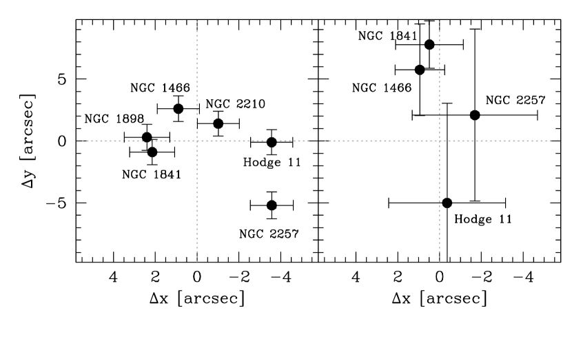
Figure 6: Left panel: Distance on the plane of the sky, along the RA and the Dec directions ($\Delta x$ and $\Delta y$, respectively), between the cluster centers estimated by MG03 (see their Table 4) and those determined in the present work (Table 2). Right panel: The same as in the left panel for the four GCs in common with S18 (see their Table 2).

Table 2: Center of gravity

Cluster	RA	Dec	$\sigma_{\rm rms}$
NGC 1466	$03^{\rm h}$ $44^{\rm m}$ $32.71^{\rm s}$	$-71\arcdeg$ $40\arcmin$ $15.6\arcsec$	$0.3\arcsec$
NGC 1841	$04^{\rm h}$ $45^{\rm m}$ $22.53^{\rm s}$	$-83\arcdeg$ $59\arcmin$ $55.1\arcsec$	$0.4\arcsec$
NGC 1898	$05^{\rm h}$ $16^{\rm m}$ $41.94^{\rm s}$	$-69\arcdeg$ $39\arcmin$ $25.3\arcsec$	$0.5\arcsec$
NGC 2210	$06^{\rm h}$ $11^{\rm m}$ $31.69^{\rm s}$	$-69\arcdeg$ $07\arcmin$ $18.4\arcsec$	$0.1\arcsec$
NGC 2257	$06^{\rm h}$ $30^{\rm m}$ $12.65^{\rm s}$	$-64\arcdeg$ $19\arcmin$ $36.8\arcsec$	$0.5\arcsec$
Hodge 11	$06^{\rm h}$ $14^{\rm m}$ $22.99^{\rm s}$	$-69\arcdeg$ $50\arcmin$ $49.9\arcsec$	$0.2\arcsec$

4 Star count density profiles

To determine the projected density profile of each cluster we used the same “representative samples” of stars discussed above, and number counts corrected following the completeness curves obtained at different radial distances from the center. We divided the field of view observed in the direction of each cluster in a number of concentric annuli (typically 10-20) centered on $C_{\rm grav}$ and split in (typically four) sub-sectors. We then counted the completeness-corrected number of stars lying within each sub-sector and divided it by the sub-sector area. The stellar density in each annulus was finally obtained as the average of the sub-sector densities, and the standard deviation among the sub-sectors densities was adopted as error. To also take into account the completeness uncertainty, we repeated the procedure two more times, by correcting the number counts according to the curves obtained after the subtraction and the addition of the completeness uncertainties to the radial completeness curves obtained from the artificial star experiments. The final error bar of the projected density at every radial bin is thus assumed to span the entire range covered by the errors of the three resulting profiles. For all the clusters but NGC 1898, we performed the analysis also on the nearby fields sampled by the parallel observations, using the same magnitude thresholds adopted for the cluster populations, taking advantage of the fact that the cluster and parallel pointings have the $V$ filter in common.

The resulting stellar density profiles $\Sigma_{*}(r)$, in units of number of stars per square arcsecond, are shown in Figures 7–9 for the six program clusters (grey circles). The constant values observed at large radii correspond to the LMC field density. As expected from Figure 5, the field contribution is particularly high in the case of NGC 1898. For each cluster, we thus averaged the densities observed in the external plateau and subtracted this value (short-dashed lines in Figures 7–9) from the observed density distribution. The true cluster density profile, obtained after subtraction of the LMC background, is finally shown with black circles in the figures. As apparent, in the inner regions (where the cluster density is much larger than the field one), the background-subtracted profile remains unchanged with respect to the observed distribution. This holds for the entire radial range sampled in NGC 1466, NGC 1841 and NGC 2257, because the field density is orders of magnitude lower than the outermost value measured from the cluster pointings. For the other clusters, instead, the background subtraction significantly reduces the density in the outer portion of the profile, where the LMC contribution become increasingly more important. Indeed, after background subtraction, the external cluster density can be significantly lower than the observed LMC field level. Hence, an accurate measure of the background contribution in the direction of each cluster is crucial for a reliable determination of the outermost portion (and thus the overall shape) of the density profile.

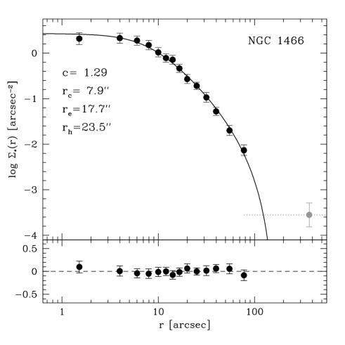
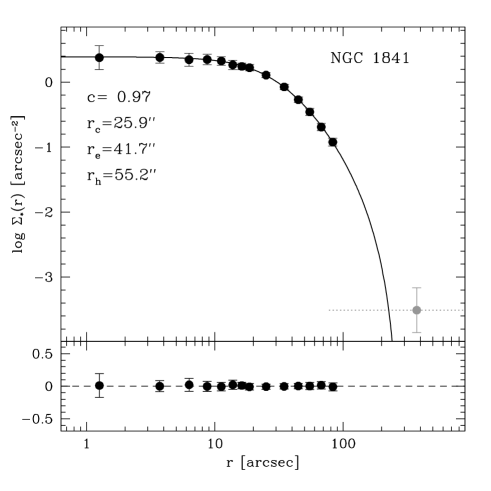
Figure 7: Projected density profiles of NGC 1466 (left) and NGC 1841 (right) obtained in the present work from resolved star counts. The black circles correspond to the cluster density profile obtained after subtraction of the LMC field contribution (grey circles and dotted lines). The black lines show the best-fit King model profiles, with the corresponding values of the concentration parameter ($c$) and a few characteristic scale-lengths (in arcseconds) labelled. The residuals between the model and the observations are plotted in the bottom portion of each panel.

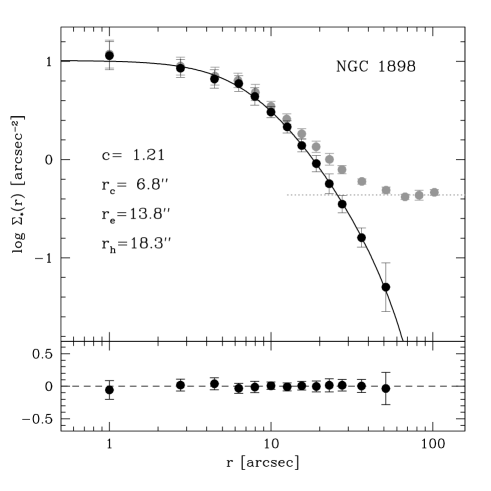
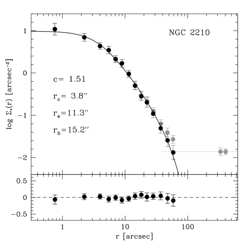
Figure 8: As in Figure 7, but for NGC 1898 and NGC 2210.

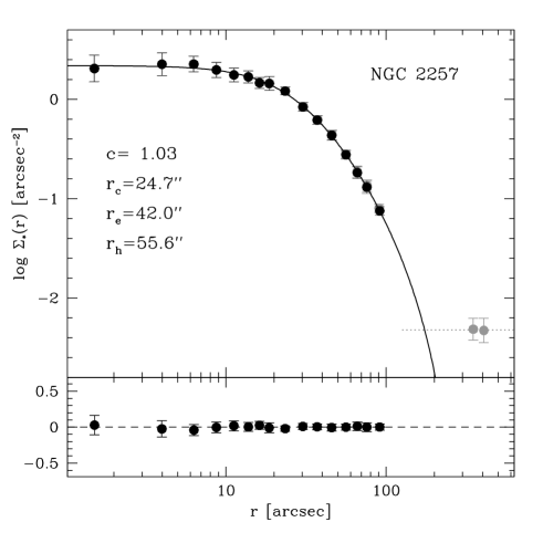
Figure 9: As in Figure 7, but for NGC 2257 and Hodge 11.

5 Models

By construction, the “reference samples” used to build the density profiles include approximately equal-mass stars, In fact, the difference in mass between objects at the MS-TO level or just below it, and those evolving in any post-MS evolutionary phases is very small (within a few 0.01 $M_{\odot}$). Hence, to determine the physical parameters of the program clusters we used single-mass, spherical and isotropic King (1966) models. This is a single-parameter family, where the shape of the density profile is uniquely determined by the dimensionless parameter $W_{0}$, which is proportional to the central gravitational potential of the system. These models are characterized by a constant projected density in the innermost region (corresponding to the so-called cluster “core”) and a decreasing behavior outwards. In practice, the higher is $W_{0}$, the smaller is the cluster core with respect to the overall size of the system. Indeed, there is a one-to-one relation between $W_{0}$ and the concentration parameter $c$, defined as $c\equiv\log(r_{t}/r_{0})$, where $r_{t}$ is the tidal (or truncation) radius of the system and $r_{0}$ is the model radial scale (the so called “King radius”). Hence, the King models are often equivalently parametrized in terms of either $W_{0}$, or $c$.

To determine the best-fit model for each of the surveyed clusters, we compared the background-subtracted surface density profiles with the King model family, leaving $W_{0}$ to vary from 4.0 to 12.0 in steps of 0.05 (the corresponding concentration parameter $c$ varies between 0.84 and 2.74). For every explored value $W_{0,i}$, we determined the scale parameter $r_{0,i}$ and the central surface density $\Sigma_{*0,i}$ providing the minimum reduced $\chi^{2}$ of the residuals between the observed and the model profiles ($\chi^{2}_{{\rm min},i}$). The solution corresponding to the lowest value of the stored $\chi^{2}_{{\rm min},i}$ ($\chi^{2}_{\rm best}$) is finally adopted as the best-fit model. Beside the best-fit values of $W_{0}$, $r_{0}$ and $\Sigma_{*0}$, this also provides several characteristic scale-lengths useful for the physical description of the cluster structure, as (see, e.g., Miocchi et al. 2013): the “core radius” ($r_{c}$), which is operatively defined as the radius at which the projected stellar density $\Sigma_{*}(r)$ drops to half of its central value (in other studies the surface brightness is considered instead of $\Sigma_{*}$; this scale-length is not equivalent to the King radius $r_{0}$, although they become increasingly similar for increasing $W_{0}$ or $c$); the “half-mass radius” ($r_{h}$), which is the radius of the sphere containing half the total cluster mass (of course, observations does not provide this 3-dimensional quantity); the “effective radius” ($r_{e}$), which is the radius of the circle that, in projection, includes half the total counted stars (in studies using the surface brightness instead of number counts, this is the radius containing half the total luminosity in projection).

The best-fit models are shown as black lines in Figures 7-9, and their residuals with respect to the observed profiles are plotted in the bottom panels. Table 3 lists the best-fit parameters together with their uncertainties estimated from the maximum variations of each parameter within the subset of models that provide a $\chi^{2}_{{\rm min},i}\leq\chi^{2}_{\rm best}+1$ (see Mv05, Miocchi et al., 2013). For each scale radius we also quote the value in parsec, computed by assuming a distance of 50 kpc for the LMC (Pietrzyński et al., 2013).

Table 3: Structural parameters

Cluster	$c$	$r_{c}$	$r_{e}$	$r_{h}$	$r_{t}$	$r_{c}$	$r_{e}$	$r_{h}$	$r_{t}$
		[$\arcsec$]	[$\arcsec$]	[$\arcsec$]	[$\arcsec$]	[pc]	[pc]	[pc]	[pc]
NGC 1466	$1.29^{+0.09}_{-0.07}$	$7.9^{+0.8}_{-0.8}$	$17.7^{+0.2}_{-0.1}$	$23.5^{+0.3}_{-0.1}$	$167.0^{+16.7}_{-10.4}$	$1.9^{+0.2}_{-0.2}$	$4.3^{+0.1}_{-0.1}$	$5.7^{+0.1}_{-0.1}$	$40.5^{+4.0}_{-2.5}$
NGC 1841	$0.97^{+0.12}_{-0.13}$	$25.9^{+1.6}_{-0.9}$	$41.7^{+3.4}_{-1.9}$	$55.2^{+4.7}_{-2.7}$	$278.4^{+66.6}_{-47.2}$	$6.3^{+0.4}_{-0.2}$	$10.1^{+0.8}_{-0.5}$	$13.4^{+1.1}_{-0.7}$	$67.5^{+16.1}_{-11.4}$
NGC 1898	$1.21^{+0.13}_{-0.11}$	$6.8^{+0.6}_{-0.6}$	$13.8^{+0.7}_{-0.4}$	$18.3^{+1.0}_{-0.6}$	$119.3^{+23.3}_{-17.2}$	$1.6^{+0.1}_{-0.1}$	$3.3^{+0.2}_{-0.1}$	$4.4^{+0.2}_{-0.1}$	$28.9^{+5.6}_{-4.2}$
NGC 2210	$1.51^{+0.09}_{-0.07}$	$3.8^{+0.4}_{-0.4}$	$11.3^{+0.3}_{-0.2}$	$15.2^{+0.5}_{-0.3}$	$130.3^{+12.0}_{-7.5}$	$0.9^{+0.1}_{-0.1}$	$2.7^{+0.1}_{-0.1}$	$3.7^{+0.1}_{-0.1}$	$31.6^{+2.9}_{-1.8}$
NGC 2257	$1.03^{+0.11}_{-0.10}$	$24.7^{+1.4}_{-1.4}$	$42.0^{+2.0}_{-1.3}$	$55.6^{+2.7}_{-1.9}$	$299.4^{+53.3}_{-39.1}$	$6.0^{+0.3}_{-0.3}$	$10.2^{+0.5}_{-0.3}$	$13.5^{+0.7}_{-0.5}$	$72.6^{+12.9}_{-9.5}$
Hodge 11	$1.09^{+0.10}_{-0.07}$	$15.0^{+0.8}_{-1.0}$	$27.1^{+1.0}_{-0.5}$	$35.9^{+1.4}_{-0.7}$	$207.0^{+32.4}_{-19.4}$	$3.6^{+0.2}_{-0.2}$	$6.6^{+0.2}_{-0.1}$	$8.7^{+0.3}_{-0.2}$	$50.2^{+7.9}_{-4.7}$

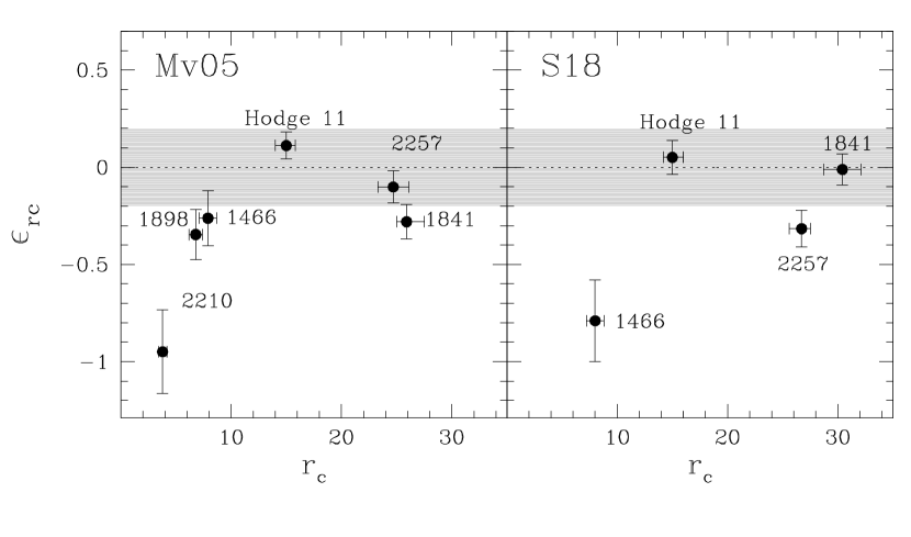
Figure 10: Comparison between the values of the King core radii determined here, and those quoted in Mv05 (left) and in S18 (right). The x-axis shows the value of $r_{c}$, in arcseconds, estimated in the present work. The y-axis corresponds to the relative difference $\epsilon_{rc}=(r_{c}-r_{c,\rm let})/r$, where where $r_{c}$ is the value here derived, while $r_{c,\rm let}$ is the one quoted in Mv05 or S18.

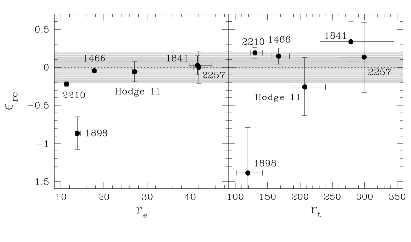
Figure 11: Comparison between the values of the King effective and tidal radii (left and right panels, respectively) determined here and in Mv05. The x-axis shows the values of $r_{e}$ and $r_{t}$, in arcseconds, estimated in the present work. The y-axis corresponds to the relative difference defined as in Figure 10, but for the effective and tidal radii, instead of $r_{c}$.

6 Discussion and conclusions

Figures 7-9 clearly show that the observed density profiles of all the investigated clusters are very well reproduced by King models. These span a large range of core radii, from just $\sim 4\arcsec$ (1 pc) for NGC 2210, up to $30\arcsec$ (7 pc) for NGC 1841, which is also the system with the lowest concentration parameter $c$.

The comparison between the scale-radii estimated in this work and those derived by Mv05 and S18 is shown in Figures 10 and 11. Mv05 used the observed surface brightness (instead of number count) profiles. S18 modeled the observed density distributions with Elson et al. (1989) models, but then listed the corresponding values of the King core radius in their Table 2. To transform into arcseconds the values that Mv05 quote in parsec we used the LMC distance adopted in their paper (50.1 kpc). The conversion of the S18 values is done by assuming the distance moduli listed in their Table 3. For each scale radius, we plot the relative difference $\epsilon_{rx}=(r_{x}-r_{x,\rm let})/r_{x}$, where $r_{x}$ is the value of $r_{c}$, $r_{e}$ or $r_{t}$ here derived, and $r_{x,\rm let}$ is the corresponding one quoted either in Mv05, or in S18 (for $r_{c}$ only). In terms of $r_{c}$, the comparison with the Mv05 values shows a good agreement for the three largest systems, while a notable discrepancy is found for NGC 2210, which is the most compact cluster ($r_{c}=4.4\arcsec$ in our study). This may be explained by noticing that the cluster center here determined is offset by almost $2\arcsec$ from the one derived by MG03 (which is also adopted by Mv05; see Fig. 6). This is indeed a large difference for such a compact cluster, and it is likely the main reason for the detected discrepancy in the value of $r_{c}$. In addition, we note that the King model fit to the surface brightness profile of NGC 2210 is rather poor in Mv05 (see the $\chi^{2}$ values in their Table 10). On the other hand, the two values of $r_{c}$ well agree for NGC 2257, in spite of a $\sim 6\arcsec$ offset between the two center estimates. This is because the cluster core is so large ($r_{c}\sim 27\arcsec$) that an error in the determination of the center has little impact on the resulting value of $r_{c}$. With respect to S18, the largest discrepancy is found for NGC 1466, while a reasonable agreement is found for the other clusters. Also in this case, NGC 1466 is the most compact systems among the four in common with S18, and the detected discrepancy may be due to a different location of the center, that in S18 is offset by $\sim 6\arcsec$ toward the north, with respect to our determination (Fig. 6). The comparison with the effective and tidal radii quoted by Mv05 (Figure 11) shows only one notable discrepancy: for NGC 1898, the Mv05 values for both the scale-lengths exceed those here determined by factors of $\sim 2$. As apparent from Figure 5, the LMC field density contribution in the direction of this cluster is very high. Hence, the detected discrepancy could be explained if Mv05 performed an insufficient subtraction of the background density from the observed (surface brightness) profile. This would, in fact, induce systematic overestimates of the large-scale radii (as $r_{e}$ and even more $r_{t}$).

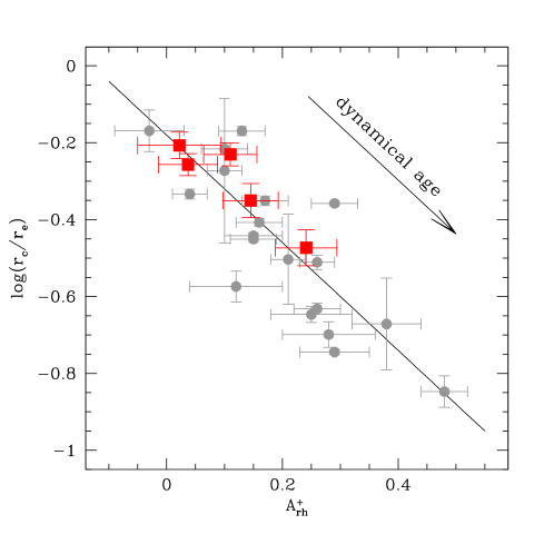
Figure 12: Relation between the $A^{+}$ parameter and the ratio between the core and the effective radii for five of the six investigated LMC clusters (all, but NGC 1898; red squares), compared to that obtained for a sample of 19 globulars in the Milky Way (grey circles). The $A^{+}$ parameter is a sensitive indicator of the level of internal dynamical evolution suffered by star clusters, its value increasing for increasing dynamical age of the system (see the arrow).

As mentioned in the Introduction, Ferraro et al. (2019) recently investigated the dynamical ages of five of the surveyed clusters (namely, NGC 1466, NGC 1841, NGC 2210, NGC 2257 and Hodge 11), by measuring the central segregation of their BSS populations through the $A^{+}$ parameter. The authors found that these five LMC old clusters reached different levels of dynamical evolution and nicely follow the relation between $A^{+}$ and $r_{c}$ drawn by the Galactic GC population. The trend is consistent with the expectations of a long-term evolution driven by two-body relaxation, with $r_{c}$ progressively decreasing in time. In turn, this implies that the large spread in core radii observed in coevally old star clusters in the LMC (e.g., MG03) can be interpreted as the natural effect of their internal dynamical evolution, which progressively moves stellar systems with relaxation times significantly shorter than their ages toward small $r_{c}$ configurations. In such a scenario, no extra energy sources (provided, e.g., by a significant population of binary black holes; Mackey et al., 2008) are required to explain the observed age-$r_{c}$ distribution in the LMC, and there is no more need of an evolutionary path where compact young clusters evolve into old globulars with a wide range of core radii (see the discussion in Ferraro et al., 2019).

The present study allows us to further investigate this issue by studying the link between the dynamical indicator $A^{+}$ and $r_{c}/r_{e}$. In fact, this ratio is expected to progressively decrease with the long-term evolution of the cluster, unless an efficient energy source intervenes to halt the core contraction and possibly even induce core expansion (e.g. Merritt et al., 2004; Baumgardt et al., 2005; Mackey et al., 2008; Trenti et al., 2010). Figure 12 shows the behavior of $r_{c}/r_{e}$ as a function of the $A^{+}$ parameter for the 5 LMC clusters in common with Ferraro et al. (2019, red squares), and for a sample of 19 Galactic GCs (grey circles) for which $A^{+}$ and $r_{e}$ have been homogeneously measured (see Miocchi et al. 2013; Lanzoni et al. 2016; Ferraro et al. 2018b). The observed trend is in perfect agreement with what shown in Figure 8 of Miocchi et al. (2013) for Milky Way GCs, and it indicates that systems characterized by large values of $r_{c}/r_{e}$ are dynamically younger than those showing small values of this ratio, as expected from a two-body relaxation driven evolution. Figure 12 also shows that no GCs with large dynamical age have a large value of $r_{c}/r_{e}$, thus further supporting the conclusion that systems with large core radii are just dynamically younger than the more compact ones, with no need of invoking anomalous energy sources able to induce core expansion. Of course, the fraction of massive dark remnants (black holes and neutron stars) retained within the cluster potential well has a significant impact in delaying the time-scale of the BSS sedimentation process (e.g., Alessandrini et al. 2016), and the measure of $A^{+}$ cannot discriminate between the presence or the absence of a large population of these objects. However, the observational evidence of significant fractions of black holes in GCs is still sparse. Therefore, it appears that the main driver of the BSS segregation process (and of the resulting value of $A^{+}$) is the long-term internal dynamical evolution of the system, while the action of dark remnants can be considered at most as a second-order effect. At this stage, the measure of the dynamical age of the most compact old LMC clusters is of utmost importance to fully confirm this scenario and to identify any system that might deviate from the trend shown in Figure 12.

References

- Alessandrini et al. (2016) Alessandrini, E., Lanzoni, B., Miocchi, P., Ferraro, F. R., & Vesperini, E. 2016, ApJ, 833, 252
- Anderson et al. (2008) Anderson, J., Sarajedini, A., Bedin, L. R., et al. 2008, AJ, 135, 2055
- Baumgardt et al. (2005) Baumgardt, H., Makino, J., & Hut, P. 2005, ApJ, 620, 238
- Baumgardt, & Hilker (2018) Baumgardt, H., & Hilker, M. 2018, MNRAS, 478, 1520
- Beccari et al. (2010) Beccari, G., Pasquato, M., De Marchi, G., et al. 2010, ApJ, 713, 194
- Beccari et al. (2019) Beccari G., Ferraro, F.R., Dalessandro, E., et al. 2019, ApJ, 876, 87
- Bellazzini et al. (2002) Bellazzini, M., Fusi Pecci, F., Messineo, M., et al. 2002, AJ, 123, 1509
- Calzetti et al. (1993) Calzetti, D., de Marchi, G., Paresce, F., & Shara, M. 1993, ApJ, 402, L1
- Cadelano et al. (2017) Cadelano, M., Dalessandro, E., Ferraro, F. R., et al. 2017, ApJ, 836, 170
- Dalessandro et al. (2008) Dalessandro, E., Lanzoni, B., Ferraro, F. R., et al. 2008, ApJ, 681, 311
- Dalessandro et al. (2013) Dalessandro, E., Ferraro, F. R., Massari, D., et al. 2013, ApJ, 778, 135
- Dalessandro et al. (2015) Dalessandro, E., Ferraro, F. R., Massari, D., et al. 2015, ApJ, 810, 40
- Dalessandro et al. (2018) Dalessandro, E., Cadelano, M., Vesperini, E., et al. 2018, ApJ, 859, 15
- Dubath et al. (1997) Dubath, P., Meylan, G., & Mayor, M. 1997, A&A, 324, 505
- Elson et al. (1989) Elson, R. A. W., Fall, S. M., & Freeman, K. C. 1989, ApJ, 336, 734
- Ferraro et al. (1997) Ferraro, F. R., Paltrinieri, B., Fusi Pecci, F., et al. 1997, A&A, 324, 915
- Ferraro et al. (1999) Ferraro, F. R., Paltrinieri, B., Rood, R. T., & Dorman, B. 1999, ApJ, 522, 983
- Ferraro et al. (2003) Ferraro, F. R., Possenti, A., Sabbi, E., et al. 2003, ApJ, 595, 179
- Ferraro et al. (2006) Ferraro, F. R., Sabbi, E., Gratton, R., et al. 2006, ApJ, 647, L53
- Ferraro et al. (2009) Ferraro, F. R., Beccari, G., Dalessandro, E., et al. 2009, Nature, 462, 1028
- Ferraro et al. (2012) Ferraro, F. R., Lanzoni, B., Dalessandro, E., et al. 2012, Nature, 492, 393
- Ferraro et al. (2018b) Ferraro, F. R., Lanzoni, B, Raso, S., et al. 2018b, ApJ, 860, 36
- Ferraro et al. (2018a) Ferraro, F. R., Mucciarelli, A., Lanzoni, B., et al. 2018a, ApJ, 860, 50
- Ferraro et al. (2019) Ferraro, F. R., Lanzoni, B., Dalessandro, E. et al. 2019, Nature Astronomy, in press
- Fiorentino et al. (2014) Fiorentino, G., Lanzoni, B., Dalessandro, E., et al. 2014, ApJ, 783, 29
- Harris (1996) Harris, W. E. 1996, AJ, 112, 1487, 2010 edition
- King (1966) King, I. R. 1966, AJ, 71, 64
- Lanzoni et al. (2007a) Lanzoni, B., Dalessandro, E., Ferraro, F. R., et al. 2007a, ApJ, 663, 267
- Lanzoni et al. (2007b) Lanzoni, B., Sanna, N., Ferraro, F. R., et al. 2007b, ApJ, 663, 1040
- Lanzoni et al. (2007c) Lanzoni, B., Dalessandro, E., Ferraro, F. R., et al. 2007c, ApJ, 668, L139
- Lanzoni et al. (2010) Lanzoni, B., Ferraro, F. R., Dalessandro, E., et al. 2010, ApJ, 717, 653
- Lanzoni et al. (2013) Lanzoni, B., Mucciarelli, A., Origlia, L., et al. 2013, ApJ, 769, 107
- Lanzoni et al. (2016) Lanzoni, B., Ferraro, F. R., Alessandrini, E., et al. 2016, ApJ, 833, L29
- Lanzoni et al. (2018a) Lanzoni, B., Ferraro, F. R., Mucciarelli, A., et al. 2018a, ApJ, 865, 11
- Lanzoni et al. (2018b) Lanzoni, B., Ferraro, F. R., Mucciarelli, A., et al. 2018b, ApJ, 861, 16
- Lugger et al. (1995) Lugger, P. M., Cohn, H. N., & Grindlay, J. E. 1995, ApJ, 439, 191
- Lützgendorf et al. (2011) Lützgendorf, N., Kissler-Patig, M., Noyola, E., et al. 2011, A&A, 533, A36
- Mackey & Gilmore (2003) Mackey, A.D., Gilmore,G.F., 2003, MNRAS, 338, 85 (MG03)
- Mackey et al. (2008) Mackey, A.D., Wilkinson, M. I., Davies, M. B., et al. 2008, MNRAS, 386, 65
- McLaughlin & van der Marel (2005) McLaughlin, D. E., & van der Marel, R. P. 2005, ApJS, 161, 304 (Mv05)
- Merritt et al. (2004) Merritt, D., Piatek, S., Portegies Zwart, S., et al. 2004, ApJ, 608, L25
- Meylan, & Heggie (1997) Meylan, G., & Heggie, D. C. 1997, A&A Rev., 8, 1
- Miocchi et al. (2013) Miocchi, P., Lanzoni, B., Ferraro, F. R., et al. 2013, ApJ, 774, 151
- Montegriffo et al. (1995) Montegriffo, P., Ferraro, F. R., Fusi Pecci, F., & Origlia, L. 1995, MNRAS, 276, 739
- Noyola, & Gebhardt (2006) Noyola, E., & Gebhardt, K. 2006, AJ, 132, 447
- Piatti et al. (2019) Piatti, A. E., Webb, J. J., & Carlberg, R. G. 2019, MNRAS, 489, 4367
- Pietrzyński et al. (2013) Pietrzyński, G., Graczyk, D., Gieren, W., et al. 2013, Nature, 495, 76
- Raso et al. (2017) Raso, S., Ferraro, F. R., Dalessandro, E., et al. 2017, ApJ, 839, 64
- Raso et al. (2019) Raso, S., Pallanca, C., Ferraro, F. R., et al. 2019, ApJ, 879, 56
- Salinas et al. (2012) Salinas, R., Jílková, L., Carraro, G., et al. 2012, MNRAS, 421, 960
- Saracino et al. (2015) Saracino, S., Dalessandro, E., Ferraro, F. R., et al. 2015, ApJ, 806, 152
- Shara et al. (1997) Shara, M. M., Saffer, R. A., & Livio, M. 1997, ApJ, 489, L59
- Sollima et al. (2017) Sollima, A., Dalessandro, E., Beccari, G., & Pallanca, C. 2017, MNRAS, 464, 3871
- Stetson (1994) Stetson, P. B. 1994, PASP, 106, 250
- Sun et al. (2018) Sun, W., Li, C., de Grijs, R., et al. 2018, ApJ, 862, 133 (S18)
- Trenti et al. (2010) Trenti, M., Vesperini, E., & Pasquato, M. 2010, ApJ, 708, 1598