Singularity Variables for Missing Energy Event Kinematics

Abstract

We discuss singularity variables which are properly suited for analyzing the kinematics of events with missing transverse energy at the LHC. We consider six of the simplest event topologies encountered in studies of leptonic $W$-bosons and top quarks, as well as in SUSY-like searches for new physics with dark matter particles. In each case, we illustrate the general prescription for finding the relevant singularity variable, which in turn helps delineate the visible parameter subspace on which the singularities are located. Our results can be used in two different ways — first, as a guide for targeting the signal-rich regions of parameter space during the stage of discovery, and second, as a sensitive focus point method for measuring the particle mass spectrum after the initial discovery.

1 Introduction

Events with missing transverse energy (MET) at the Large Hadron Collider (LHC) are of great interest to both theory and experiment. On the experimental side, the MET is a very challenging object, and a great amount of effort has gone into the proper calibration of the detector and in the evaluation of its missing energy performance in both ATLAS TheATLAScollaboration:2013oia and CMS CMS:2016ljj . On the theoretical side, events with MET are likely to hold the key to understanding some of the great unsolved puzzles of the Standard Model (SM). For example, the dark matter problem greatly motivates searches for new physics beyond the Standard Model (BSM) with dark matter candidates Feng:2010gw , which would escape the detector leaving a MET signature Hubisz:2008gg . Similarly, the flavor problem provides impetus for focusing on the third generation in the SM, where the top quark, the bottom quark and the tau lepton all have decay channels with invisible particles (neutrinos) in the final state. Finally, the $W$-bosons, whose leptonic decays exhibit a classic MET signature, have long been considered promising probes of the electroweak symmetry breaking sector Lee:1977eg ; Duncan:1985vj , and more recently have rounded out the suite of Higgs discovery channels Chatrchyan:2013iaa ; ATLAS:2014aga . Therefore, the sound theoretical understanding of the event kinematics in MET events should be a high priority.

The fundamental problem with MET events is the incomplete information about the final state, since the energies $\varepsilon_{i}$ and momenta $\vec{q}_{i}$ of the invisible particles (neutrinos or dark matter particles) are not measured. At the same time, there is partial information available in the form of the energies $e_{j}$ and momenta $\vec{p}_{j}$ of the visible final state particles, which typically are the (approximately massless) leptons, photons and/or QCD jets, but may also be massive reconstructed visible particles like a $W$-boson, a $Z$-boson or a Higgs boson. In the spirit of the simplified models approach Alves:2011wf , in what follows we shall remain agnostic about the underlying physics which might give rise to a particular event topology, and instead shall focus on the salient features of its kinematics as represented by phase space singularities. Correspondingly, we shall also ignore any secondary dynamical effects such as spin correlations, helicity suppressions, etc., since they do not affect the singular phase space features which we are interested in.

With this backdrop, we are ready to introduce the three relevant (and related) questions regarding MET events which will be addressed in this paper.

• Are there any singular features in the visible phase space of a given event topology?

• What are the relevant kinematic variables which best describe such singular features?

• What do measurements of such features tell us about the underlying mass spectrum?

Let us briefly motivate and comment on each question before proceeding to the main analysis in the following sections.

1.1 Visible phase space singularities

In this paper, we define a singularity in the visible parameter space $\{\vec{p}_{j}\}$ as a point where the event number density formally becomes infinite. The origin of such singularities is very well understood Kim:2009si ; Rujula:2011qn ; DeRujula:2012ns ; Kim:2019prx : they arise in the process of projecting the allowed region in the full phase space $\{\vec{q}_{i},\vec{p}_{j}\}$ (which does not exhibit any singularities) onto the visible subspace $\{\vec{p}_{j}\}$. Similar to the phenomenon of caustics in optics, astrophysics Sikivie:1997ng or accelerator physics Charles:2016xph , singularities are formed at points where the visible projection onto $\{\vec{p}_{j}\}$ of the allowed phase space in $\{\vec{q}_{i},\vec{p}_{j}\}$ gets folded. Mathematically this is expressed as the reduction in the rank of the Jacobian matrix of the coordinate transformation from the relevant set of kinematic constraints to $\{\vec{q}_{i}\}$ (alternatively, from the generator-level event parameters to the visible space $\{\vec{p}_{j}\}$), which is why such singularities are sometimes known as Jacobian peaks.

1.2 Singularity variables

The visible parameter space $\{\vec{p}_{j}\}$ may be parametrized simply in terms of the visible momentum components, as indicated, but it also allows infinitely many alternative re-parametrizations, involving, e.g., angles, rapidities, invariant masses, etc. An interesting question then is which of those re-parametrizations is “the best”. In his pioneering paper Kim:2009si , Kim proposed to construct an optimized one-dimensional kinematic variable, called a singularity coordinate, which is defined in terms of the measured visible momenta $\{\vec{p}_{j}\}$, plus possibly some mass parameters $\{M_{k}\}$. The latter set includes the masses $\sqrt{\varepsilon_{i}^{2}-\vec{q}_{i}^{\,2}}$ of the invisible particles in the final state, as well as the masses of any intermediate resonances in the event topology. As the name suggests, the singularity coordinate is designed to capture the singular behavior and so must satisfy the following criteria put forth in Kim:2009si : (i) it must vanish at the singularity locations; (ii) its direction must be perpendicular to the singularity hypersurface in the observable phase space $\{\vec{p}_{j}\}$; (iii) events which are equally far away from the singularity should produce the same value.

Unfortunately, Kim’s paper went largely unnoticed — in the past ten years, there have been very few explicitly worked out examples of practical significance, with the exception of two follow-up investigations by De Rujula and Galindo, who introduced and studied several different versions of a singularity coordinate for the case of single $W$ production Rujula:2011qn and $h\to WW$ DeRujula:2012ns . Our goal in this paper is to expand the set of worked out examples, on occasion taking the opportunity to point out connections to other results in the literature which have been obtained by different means. For completeness, we shall also review and further expand on the two case studies in Rujula:2011qn ; DeRujula:2012ns .

In parallel with the one-dimensional approach of a singularity variable, we shall also try to analyze and visualize the singularity hypersurface from a multi-dimensional perspective. For example, consider the classic supersymmetry (SUSY) example of a single decay chain proceeding through three successive two body decays. The relevant visible parameter space is three-dimensional and can be parametrized by the pairwise invariant masses of the final state visible particles. The singularity is then found at the two-dimensional surface boundary of the allowed region Costanzo:2009mq ; Lester:2013aaa ; Agrawal:2013uka ; Kim:2015bnd . In order to maximize the sensitivity, the experimental analysis should target this two-dimensional surface; this can be done either directly Debnath:2016mwb ; Debnath:2016gwz ; Altunkaynak:2016bqe (e.g., using Voronoi tessellations of the data Debnath:2015wra ; Debnath:2015hva ) or by means of a suitable one-dimensional singularity coordinate Debnath:2018azt .

1.3 Using singular features for particle mass measurements

As a result of the previous step, ideally we would end up with some parametric equation of the singularity hypersurface within the visible phase space

$$g(\{\vec{p}_{j}\};\{m_{j}\};\{M_{k}\})=0,$$ (1)

which contains three types of variables: the set $\{\vec{p}_{j}\}$ of measured 3-momenta of the visible final state particles, the corresponding set $\{m_{j}\}$ of their masses, which are known SM parameters, and finally, a set $\{M_{k}\}$ of mass parameters, which, depending on the circumstances, may or may not be known a priori. As already mentioned, $\{M_{k}\}$ would typically include the masses $m_{i}=\sqrt{{\cal\varepsilon}_{i}^{2}-\vec{q}_{i}^{\,2}}$ of the invisible particles in the final state. Now, if one is willing to assume that the invisible particles are all neutrinos, as is usually the case with studies of SM signatures, those masses can be safely set to zero. On the other hand, in studies of BSM signatures the invisible particles are some new dark matter particles whose masses are a priori unknown and should be explicitly retained in (1). Also included in the set $\{M_{k}\}$ are the masses of intermediate resonances, which are known if the resonance is a SM particle and unknown otherwise.

The constraint (1) can be viewed in different ways. First, the function $g$ can be regarded as a bona fide singularity coordinate in the sense of Ref. Kim:2009si . Second, given a choice of masses $\{M_{k}\}$, the constraint (1) defines the locus of points where the signal event density becomes singular (by construction), while the behavior of the background event density is typically unremarkable. Therefore, this locus of points is precisely the region of phase space which should be targeted (with suitable selection cuts) in an analysis aimed at a discovery Debnath:2018azt . Finally, we can turn the last argument around and instead of studying the phase space $\{\vec{p}_{j}\}$ for a given choice of mass parameters $\{M_{k}\}$, we can study the mass parameter space $\{M_{k}\}$ for given points in phase space as sampled by the events in the data. Correspondingly, for each event, eq. (1) can be viewed as a constraint on the allowed values of the mass parameters for which the current event would be located on a singularity hypersurface. In a companion paper Kim:2019prx , this idea was formulated as a new mass measurement method, called the “focus point method”, which was inspired by previous related work in Nojiri:2003tu ; Kawagoe:2004rz ; Cheng:2008hk ; Gripaios:2011jm ; Anagnostou:2011aa . The analysis in Kim:2019prx was illustrated with one specific event topology, dilepton $t\bar{t}$ events, and we shall now show that it is also applicable for the remaining 5 event topologies considered here.

The paper is organized as follows. In Section 2.1 we first introduce the six event topologies to be studied in this paper, along with our notation and conventions, as well as some details on our simulations. Then in Section 2.2 we flesh out the general method for deciding whether a singularity feature exists, and if so, for deriving the corresponding constraint (1). In the next five Sections 3-7, we illustrate the general method for each individual event topology. In the process, we shall sometimes rederive some existing results in the literature, albeit in a different, universal and perhaps more intuitive way. We hope that the expert reader will enjoy seeing the underlying commonality between those familiar results, as well as appreciate the novelty of the others. The novice reader is perhaps best advised to first read Refs. Kim:2009si ; Rujula:2011qn ; DeRujula:2012ns ; Kim:2019prx and be ready to consult a standard reference like Byckling:1971vca ; Barger:1987nn when necessary. Finally, in Section 8 we present our conclusions and outlook for future studies.

2 Preliminaries

2.1 Notations and Setup

The six event topologies to be considered in this paper are shown in Fig. 1, where, in accordance with the notation of Barr:2011xt , the letters p and q are reserved for denoting momenta of visible and invisible particles, respectively.

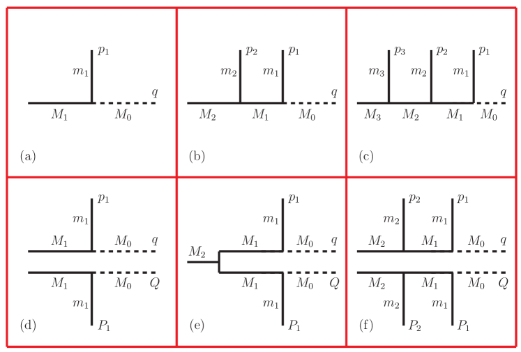
Figure 1: The event topologies studied in this paper. Diagrams (a-c) in the top row represent single decay chains, each terminating in a single invisible particle with mass $M_{0}$ and 4-momentum $q=(\varepsilon,\vec{q})$, while diagrams (d-f) in the bottom row represent pair-production processes leading to two decay chains and two invisible particles with 4-momenta $q=(\varepsilon,\vec{q})$ and $Q=({\cal E},\vec{Q})$, respectively. $p_{i}=(e_{i},\vec{p}_{i})$ and $P_{i}=(E_{i},\vec{P}_{i})$ label the 4-momenta of visible final state particles of mass $m_{i}$, while $M_{k}$ with $k=1,2,3$ label the masses of on-shell intermediate resonances.

Diagrams (a-c) in the top row represent single decay chains, each terminating in a single invisible particle with mass $M_{0}$ and 4-momentum $q=(\varepsilon,\vec{q})$, which is taken to be on-shell: $\varepsilon^{2}-\vec{q}^{\,2}=M_{0}^{2}$. The decay chains in Fig. 1(a-c) differ by the number of two-body decays — here we have limited ourselves to at most three (in Fig. 1(c)), but the generalization to four or more is straightforward Altunkaynak:2016bqe . Similarly, $p_{i}=(e_{i},\vec{p}_{i})$, with $i=1,2,3$, label the 4-momenta of visible final state particles of mass $m_{i}$, with $e_{i}^{2}-\vec{p}_{i}^{\,2}=m_{i}^{2}$. The masses $M_{k}$ with $k=1,2,3$ label the masses of on-shell intermediate resonances. The diagrams (d-f) in the bottom row of Fig. 1 represent pair-production processes leading to two decay chains and thus to two invisible particles with 4-momenta $q=(\varepsilon,\vec{q})$ and $Q=({\cal E},\vec{Q})$, respectively. The 4-momenta of the visible particles in the second decay chain are similarly capitalized: $P_{i}=(E_{i},\vec{P}_{i})$, where $E_{i}^{2}-\vec{P}_{i}^{\,2}=m_{i}^{2}$ and $i=1,2$.

The six diagrams in Fig. 1 cover a host of interesting physics processes at the LHC, both within and outside the SM. For any given such process, there will be a corresponding choice for the masses $m_{i}$, $M_{0}$ and $M_{k}$. Consider, for example, single top decay

$$t\to bW^{+}\to b\ell^{+}\nu$$ (2)

as an illustration for Fig. 1(b). In that case, $m_{1}$ is the mass of a lepton (electron or muon), $m_{2}$ is the mass of the reconstructed $b$-jet, $M_{0}$ is the neutrino mass, $M_{1}$ is the $W$-boson mass and $M_{2}$ is the top quark mass. Any other process will dictate a similar choice of mass parameters; and of course, BSM processes may involve dark matter particles and intermediate resonances with a priori unknown masses $M_{0}$ and $M_{k}$. In order to keep everything on the same footing, in our numerical examples we shall use the same mass spectrum for all six processes as shown in Table 1.

Parameter	$M_{0}$	$M_{1}$	$M_{2}$	$M_{3}$
Value (in GeV)	700	800	1000	1300

Table 1: The common mass spectrum used in the numerical examples, except for Fig. 1(e) where $M_{2}=3000$ GeV instead.

Events will be generated at parton level with MadGraph Alwall:2011uj . Intermediate resonances will be decayed by phase space, i.e., ignoring any spin correlations. This assumption will not impact our results, since they are based on purely kinematics arguments and are thus independent of the model dynamics. For clarity of the presentation, and to better see the singularity structures, we will not employ any detector simulation and will keep the intermediate resonances strictly on-shell. Of course, in a real experiment there will be some smearing due to both the detector resolution and the finite particle widths; the extent of those effects depends on the particular realization of the topology in question and is beyond our scope here. The visible final state particles, which are typically leptons and QCD jets, will be taken to be massless. As we shall see below, in the case of Fig. 1(a), the presence of initial state radiation (ISR) is important and actually quite beneficial for the analysis. This is why ISR will be simulated for that case, while in the remaining event topologies the ISR will not be modelled. Finally, we shall ignore the combinatorial problem arising in Fig. 1(f), since it has already been addressed in the literature Baringer:2011nh ; Choi:2011ys ; Debnath:2017ktz , and for simplicity we will assume that the visible particles have been properly assigned to the two decay branches.

2.2 The basic idea

We are now ready to outline the general method for deriving a singularity variable Kim:2009si ; Rujula:2011qn ; DeRujula:2012ns ; Kim:2019prx . The first step is to collect all kinematic constraints on the invisible momenta $q$ (and $Q$, if applicable). In general, the kinematic constraints fall into several categories:

• On-shell relations. These exist for the final state invisible particles

  $$M_{0}^{2} = q^{2},$$ (3a)

  $$M_{0}^{2} = Q^{2},$$ (3b)

  as well as for the intermediate resonances:

  $$M_{k}^{2} = \left(q+\sum_{i=1}^{k}p_{i}\right)^{2},$$ (4a)

  $$M_{k}^{2} = \left(Q+\sum_{i=1}^{k}P_{i}\right)^{2}.$$ (4b)

  Notice that the equations (3b) and (4b) are only applicable in the case of the bottom row diagrams in Fig. 1.

• Missing transverse momentum constraint. Momentum conservation in the transverse plane constrains the sum of the transverse momenta of the invisible particles:

  $${\;/\!\!\!\!\vec{P}_{T}}=\left\{\begin{array}[]{ll}\vec{q}_{T}&\text{\rm for\ Fig.~{}\ref{fig:feynmandiag}(a-c),}\\[5.69054pt] \vec{q}_{T}+\vec{Q}_{T}&\text{\rm for\ Fig.~{}\ref{fig:feynmandiag}(d-f).}\end{array}\right.$$ (5)

• Additional constraints due to the specific experimental setup. Additional constraints may arise at specific experimental facilities, e.g., at a lepton collider, where the center-of-mass (CM) energy and momentum of the initial state are known.

Combining all of these constraints, we obtain a set of $N_{C}$ equations

$$f_{\alpha}\left(\left\{p,P\right\};\left\{q,Q\right\};\left\{M_{k}\right\}\right)=0,\qquad\alpha=1,2,....,N_{C},$$ (6)

involving the set $\left\{p,P\right\}$ of measured 4-momenta of the visible final state particles, the unknown 4-momenta $\left\{q,Q\right\}$ of the invisible final state particles, and the set of mass parameters $\left\{M_{k}\right\}$ introduced in Section 1.2. For the single decay chain diagrams in the top row of Fig. 1, the momenta $P_{i}$ and $Q$ are absent, and (6) simplifies to

$$f_{\alpha}\left(\left\{p\right\};\left\{q\right\};\left\{M_{k}\right\}\right)=0,\qquad\alpha=1,2,....,N_{C}.$$ (7)

Let $N_{q}$ be the total number of invisible 4-momentum components, i.e.

$$N_{q}=\left\{\begin{array}[]{ll}4,{}{}&{\rm for\ the\ case\ of\ Figs.~{}\ref{fig:feynmandiag}(a-c)},\\ 8,{}{}&{\rm for\ the\ case\ of\ Figs.~{}\ref{fig:feynmandiag}(d-f)}.\end{array}\right.$$ (8)

In what follows, we shall focus on situations where the number of constraints $N_{C}$ is just enough so that one can solve (6) and (7) for the invisible momenta in terms of the mass parameters $\left\{M_{k}\right\}$. In other words we shall always have

$$N_{C}=N_{q}.$$ (9)

Note that this does not imply that the final state kinematics is fully solved — we are just trading one set of unknowns, the components of the invisible momenta, for another: the masses $\left\{M_{k}\right\}$ of the intermediate resonances and of the invisible final state particles. In other words, we are still dealing with an undetermined problem, in which we are not able to compute the exact momenta of the invisible particles in the event.

In order to illustrate the basic idea, it is sufficient to consider the simpler version (7) of the kinematic constraints — the same argument goes through for any number of invisible particles in the final state, as long as (9) is in effect. Consider some particular solution $\tilde{q}^{\mu}$ of (7):

$$f_{\alpha}\left(\left\{p\right\};\left\{\tilde{q}\right\};\left\{M_{k}\right\}\right)=0,\qquad\alpha=1,2,....,N_{C}.$$ (10)

A singularity at $\tilde{q}$ is obtained when at least one of the directions of the local tangent plane to the full phase space is aligned with an invisible momentum direction Kim:2009si . This means that we can make an infinitesimal change $\delta\tilde{q}$ in the unmeasured invisible 4-momentum components while continuing to satisfy the original system, i.e.

$$f_{\alpha}\left(\left\{p\right\};\left\{\tilde{q}+\delta\tilde{q}\right\};\left\{M_{k}\right\}\right)=0,\qquad\alpha=1,2,....,N_{C}.$$ (11)

Upon expanding the last equation and taking into account (10), one finds

$$\frac{\partial f_{\alpha}}{\partial q^{\mu}}\ \delta\tilde{q}^{\mu}=0,\qquad\alpha=1,2,....,N_{C}.$$ (12)

The condition (9) ensures that the Jacobian matrix

$$D_{\alpha\mu}\equiv\frac{\partial f_{\alpha}}{\partial q^{\mu}}$$ (13)

is a square matrix. The existence of non-trivial solutions $\delta\tilde{q}^{\mu}$ for the system (12) is guaranteed if the determinant of $D_{\alpha\mu}$ vanishes:

$${\rm Det}\,D_{\alpha\mu}(\left\{p\right\},\left\{M_{k}\right\})\equiv\left|\frac{\partial f_{\alpha}}{\partial q^{\mu}}\right|_{q=\tilde{q}}=0.$$ (14)

Note that the left-hand side of this equation is a function of only visible momenta $\left\{p\right\}$ and mass parameters $\left\{M_{k}\right\}$, since the invisible momenta can be eliminated via eqs. (10). Comparing to (1), we see that the left-hand side of (14) can be taken to be the desired singularity coordinate. Repeating the same argument for the case with two invisible particles, i.e., starting from eq. (6), leads us to a similar condition

$$\left|\frac{\partial f_{\alpha}}{\partial(q,Q)}\right|=0.$$ (15)

From a mathematical point of view, eqs. (14) and (15) are simply the reduced rank conditions leading to a critical point. In our case their importance lies in the fact that the distribution of the corresponding kinematic variable is singular at the critical point, which is why Refs. Rujula:2011qn ; DeRujula:2012ns also referred to these reduced rank conditions as “singularity conditions”.

In the subsequent sections we shall explore the implication of (14) or (15) for the event topologies of Fig. 1. As outlined in the introduction, for each event topology we shall focus on the following three issues:

• Derivation of the relevant singularity coordinate.

• Delineation of the signal-rich regions of the visible phase space, i.e., where the signal density becomes singular. In doing so, we shall be careful to use the symmetries of the problem in order to maximally reduce the dimensionality of the observable phase space without washing out any singular kinematic features.

• Demonstration of the focus point method for mass measurements proposed in Kim:2019prx .

3 Single decay chain, one two-body decay

In this section we shall consider the single two-body decay diagram from Fig. 1(a). We shall revisit and expand the discussion in Ref. Rujula:2011qn , which showed that the singularity coordinate in this case is nothing but the usual transverse mass variable $m_{T}$ Barger:1983wf ; Smith:1983aa . By now, the transverse mass is one of the standard kinematic variables, which has been widely used in precision measurements of the $W$-boson mass Abazov:2012bv ; Aaltonen:2013vwa ; Aaboud:2017svj as well as in new physics searches for $W^{\prime}$ resonances Abazov:2007ah ; Aaltonen:2010jj ; Sirunyan:2018mpc ; Aad:2019wvl . The new element in our discussion will be the role of the focus point method of Kim:2019prx and its connection to the kink method for mass measurements Cho:2007qv ; Gripaios:2007is ; Barr:2007hy ; Cho:2007dh ; Matchev:2009fh .

3.1 Derivation of a singularity coordinate

Let us begin by listing the four kinematic constraints for Fig. 1(a):

$$q^{2} = M_{0}^{2},$$ (16a)

$$(q+p_{1})^{2} = M_{1}^{2},$$ (16b)

$$\vec{q}_{T} = {\;/\!\!\!\!\vec{P}_{T}},$$ (16c)

or after a simple rearrangement,

$$q^{2} = M_{0}^{2},$$ (17a)

$$2p_{1}\cdot q = M_{1}^{2}-M_{0}^{2}-m_{1}^{2},$$ (17b)

$$q_{x} = {\;/\!\!\!\!P_{x}},$$ (17c)

$$q_{y} = {\;/\!\!\!\!P_{y}}.$$ (17d)

The Jacobian matrix (13) in this case is Rujula:2011qn

$$D=\left(\begin{array}[]{cccc}2\varepsilon&-2q_{x}&-2q_{y}&-2q_{z}\\ 2e_{1}&-2p_{1x}&-2p_{1y}&-2p_{1z}\\ 0&1&0&0\\ 0&0&1&0\end{array}\right)$$ (18)

and the corresponding singularity condition (14) reads Rujula:2011qn

$${\rm Det}\,D=-4(\varepsilon p_{1z}-e_{1}q_{z})=0.$$ (19)

The latter is nothing but the equal rapidity condition

$$\frac{\varepsilon}{q_{z}}=\frac{e_{1}}{p_{1z}},$$ (20)

which is known Barr:2011xt to provide the link between transverse invariant mass variables (like the transverse mass $m_{T}$, the Cambridge $m_{T2}$ and others) and their respective 3+1 dimensional analogues Ross:2007rm ; Barr:2008ba ; Konar:2008ei ; Konar:2010ma ; Mahbubani:2012kx ; Cho:2014naa ; Cho:2014yma ; Kim:2014ana ; Swain:2014dha ; Cho:2015laa ; Konar:2016wbh ; Goncalves:2018agy . In order to cast the singularity condition in the desired form (1), we must eliminate the invisible 4-momentum $q$ by using four out of the five equations appearing in eqs. (17) and (20). For example, using (17a), (17c), (17d) and (20), one can find the components of the 4-vector $q=(\varepsilon,q_{x},q_{y},q_{z})$ as

$$\varepsilon = e_{1}\,\sqrt{\frac{M_{0}^{2}+{\;/\!\!\!\!P_{T}^{2}}}{m_{1}^{2}+p_{1T}^{2}}},$$ (21a)

$$q_{x} = {\;/\!\!\!\!P_{x}},$$ (21b)

$$q_{y} = {\;/\!\!\!\!P_{y}},$$ (21c)

$$q_{z} = p_{1z}\,\sqrt{\frac{M_{0}^{2}+{\;/\!\!\!\!P_{T}^{2}}}{m_{1}^{2}+p_{1T}^{2}}}.$$ (21d)

Substituting the result (21) into the remaining fifth equation (17b), we obtain the final singularity condition explicitly in the form

$$m_{1}^{2}+M_{0}^{2}+2\left(\sqrt{m_{1}^{2}+p_{1T}^{2}}\sqrt{M_{0}^{2}+{\;/\!\!\!\!P_{T}^{2}}}-\vec{p}_{1T}\cdot{\;/\!\!\!\!\vec{P}_{T}}\right)-M_{1}^{2}=0,$$ (22)

where in the left-hand side we recognize the transverse mass variable $m_{T}$ written as

$$m^{2}_{T}(M_{0})\equiv m_{1}^{2}+M_{0}^{2}+2\left(\sqrt{m_{1}^{2}+p_{1T}^{2}}\sqrt{M_{0}^{2}+{\;/\!\!\!\!P_{T}^{2}}}-\vec{p}_{1T}\cdot{\;/\!\!\!\!\vec{P}_{T}}\right).$$ (23)

If we introduce the transverse energies

$$e_{1T} \equiv \sqrt{m_{1}^{2}+p_{1T}^{2}},$$ (24)

$$\varepsilon_{T} \equiv \sqrt{M_{0}^{2}+{\;/\!\!\!\!P_{T}^{2}}},$$ (25)

the previous result (23) can be rewritten more compactly in the familiar form Barger:1987nn

$$m^{2}_{T}(M_{0})=\left[e_{1T}+\varepsilon_{T}(M_{0})\right]^{2}-\left[\vec{p}_{1T}+{\;/\!\!\!\!\vec{P}_{T}}\right]^{2}.$$ (26)

Note that while we have succeeded in eliminating the unknown components of the invisible 4-momentum $q$, there still remains one a priori unknown parameter, namely, the mass $M_{0}$ of the invisible particle, which enters through the transverse energy $\varepsilon_{T}$. The singularity condition (22) can then be rewritten in the very compact form

$$m_{T}(M_{0})=M_{1}.$$ (27)

This confirms that, up to the additive constant $M_{1}$, the relevant singularity variable for the event topology of Fig. 1(a) is indeed the transverse mass $m_{T}$. Furthermore, eq. (27) shows that the singularity occurs at the mass $M_{1}$ of the parent particle, i.e.

$$\lim_{m_{T}\to M_{1}}\left(\frac{dN}{dm_{T}}\right)=\infty.$$ (28)

However, there is an important subtlety — the latter statement is true only if we have made the correct choice for the invisible mass parameter $M_{0}$ entering the definition (26). In general, the true value of $M_{0}$ is a priori unknown, and we have to adopt a certain ansatz for it (denoted in the following by $\tilde{M}_{0}$) in order to compute the transverse mass $m_{T}$ from (26). Once the ansatz $\tilde{M}_{0}$ differs from the true value $M_{0}$, the existence of a singularity in the $m_{T}(\tilde{M}_{0})$ distribution is generally not guaranteed, and the singular feature in the $dN/dm_{T}$ distribution predicted by eqs. (27) and (28) will be washed out. This is the key observation behind the focus point method for mass measurements proposed in Kim:2019prx . There the method was illustrated for the case of the dilepton $t\bar{t}$ event topology of Fig. 1(f). In Sec. 3.3 below we shall show that it is also applicable to the simple event topology of Fig. 1(a) as well. But first let us understand the phase space geometry behind the singularity condition (27).

3.2 The phase space geometry of the singularity condition

In general, the parent particle is produced inclusively, and the event depicted in Fig. 1(a) would also contain additional visible particles due to initial state radiation (ISR), or decays upstream to the parent particle. Let us denote the total transverse momentum of these additional visible particles as $\vec{P}_{T}^{ISR}$, which can be measured in the detector. Then, by definition, the missing transverse momentum ${\;/\!\!\!\!\vec{P}_{T}}$ is due to the invisible recoil against both $\vec{p}_{1T}$ and $\vec{P}_{T}^{ISR}$:

$${\;/\!\!\!\!\vec{P}_{T}}\equiv-\vec{p}_{1T}-\vec{P}_{T}^{ISR}.$$ (31)

3.2.1 The case of no upstream visible momentum: $P_{T}^{ISR}=0$

In order to gain some intuition, it is instructive to first consider the simpler case of no upstream visible momentum, $P_{T}^{ISR}=0$. In that case, (31) reduces to ${\;/\!\!\!\!\vec{P}_{T}}=-\vec{p}_{1T}$ and the transverse mass (26) can be written simply as

$$m_{T}(\tilde{M}_{0})=e_{1T}+\varepsilon_{T}(\tilde{M}_{0})=\sqrt{m_{1}^{2}+p_{1T}^{2}}+\sqrt{\tilde{M}_{0}^{2}+p_{1T}^{2}}.$$ (32)

Note that in this case $m_{T}$ is a function of only one degree of freedom, namely, the magnitude of $\vec{p}_{1T}$. This can be easily understood in terms of the symmetries of the problem — $p_{1z}$ does not enter due to the invariance under longitudinal boosts, while the direction of $\vec{p}_{1T}$ is irrelevant due to the azimuthal symmetry.

The singularity condition (27) can then be written as

$$\sqrt{m_{1}^{2}+p_{1T}^{2}}+\sqrt{M_{0}^{2}+p_{1T}^{2}}=M_{1}.$$ (33)

The set of points satisfying this relation belong to a circle in the $\vec{p}_{1T}$ plane which is centered at the origin and has radius equal to

$$p_{1T}^{max}=\frac{\sqrt{\lambda(M_{1}^{2},M_{0}^{2},m_{1}^{2})}}{2M_{1}},$$ (34)

where $\lambda(x,y,z)\equiv x^{2}+y^{2}+z^{2}-2xy-2xz-2yz$. Such points were categorized as “extreme” in Kim:2019prx , since they delineate the boundary of the allowed phase space, where the solutions for the invisible momenta become degenerate. This is pictorially illustrated in Fig. 2, where the top left panel corresponds to the current case of $P_{T}^{ISR}=0$.

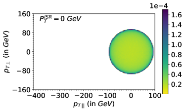
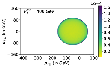
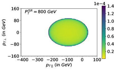
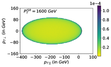
Figure 2: Allowed values for the transverse momentum of the visible particle (assumed massless for simplicity) for different values of $P_{T}^{ISR}$: $P_{T}^{ISR}=0$ (top left), $P_{T}^{ISR}=400$ GeV (top right), $P_{T}^{ISR}=800$ GeV (bottom left) and $P_{T}^{ISR}=1600$ GeV (bottom right). Following Refs. Matchev:2009ad ; Konar:2009wn , the component in the direction of $\vec{P}_{T}^{ISR}$ is denoted by $p_{T\parallel}$ and defined in (38), while the component in a direction orthogonal to $\vec{P}_{T}^{ISR}$ is denoted by $p_{T\perp}$ and defined in (39). The color scale is indicative of the event number density. In particular, points colored in deep purple mark the locations in phase space where the number density becomes singular.

We plot the event number density (as indicated by the color bar) in the $\vec{p}_{1T}$ plane, which we choose to parametrize as $(p_{T\parallel},p_{T\perp})$, where $p_{T\parallel}$ ($p_{T\perp}$) is the component in the direction along (orthogonal to) $\vec{P}_{T}^{ISR}$ Matchev:2009ad ; Konar:2009wn . We see that the allowed phase space in the $\vec{p}_{1T}$ plane is indeed a circle, and furthermore, that the maximal event density is found along the circumference of the circle, in agreement with (33). With the mass spectrum from Table 1, eq. (34) predicts the radius of the circle to be $p_{1T}^{max}=93.75$ GeV, which is confirmed in the top left panel of Fig. 2. Since the extreme events along the circumference of the circle have the same value of $p_{1T}=p_{1T}^{max}$, they will also share the same value of $m_{T}$, regardless of the choice of test mass $\tilde{M}_{0}$, see eq. (32). This means that for any value of $\tilde{M}_{0}$, the $m_{T}(\tilde{M}_{0})$ distribution will continue to exhibit a singularity at

$$m_{T}^{max}(\tilde{M}_{0})=\sqrt{m_{1}^{2}+(p_{1T}^{max})^{2}}+\sqrt{\tilde{M}_{0}^{2}+(p_{1T}^{max})^{2}}.$$ (36)

This is illustrated explicitly in Fig. 3, which shows several unit-normalized distributions of the transverse mass (32) for the case of $P_{T}^{ISR}=0$ and with the mass spectrum from Table 1 ($M_{1}=800$ GeV and $M_{0}=700$ GeV). The test mass is chosen as $\tilde{M}_{0}=0$ GeV in the left panel, $\tilde{M}_{0}=700$ GeV in the middle panel and $\tilde{M}_{0}=1400$ GeV in the right panel. We see that in all three cases, the $m_{T}$ distribution has a very sharp singularity at its upper kinematic endpoint (36).

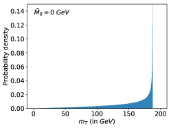
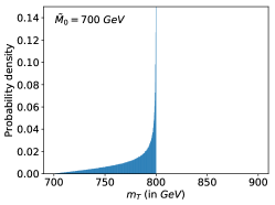
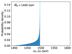
Figure 3: Unit-normalized distributions of the relevant transverse mass (32) for the case of $P_{T}^{ISR}=0$ and with the mass spectrum from Table 1: $M_{1}=800$ GeV and $M_{0}=700$ GeV. The test mass is chosen as $\tilde{M}_{0}=0$ GeV (left panel), $\tilde{M}_{0}=700$ GeV (middle panel) and $\tilde{M}_{0}=1400$ GeV (right panel). In each case, the upper kinematic endpoint of the $m_{T}$ distribution is given by (36).

However, this situation is rather atypical — we shall see below that, in general, when we use the wrong value for the invisible mass parameter $\tilde{M}_{0}$, the singularity will be washed out. The reason why it persists here is that the singularity coordinate (32) is parametrized by a single degree of freedom, $p_{1T}$.

3.2.2 The case with non-zero upstream visible momentum: $P_{T}^{ISR}\neq 0$

We are now in position to discuss the more general case of non-vanishing upstream visible momentum, $\vec{P}_{T}^{ISR}\neq 0$. Using (31), the transverse mass formula (26) becomes Barr:2011xt

$$m^{2}_{T}(\tilde{M}_{0})=\left[\sqrt{m_{1}^{2}+p_{1T}^{2}}+\sqrt{\tilde{M}_{0}^{2}+(\vec{p}_{1T}+\vec{P}_{T}^{ISR})^{2}}\right]^{2}-(P_{T}^{ISR})^{2}.$$ (37)

Since $\vec{P}_{T}^{ISR}$ breaks the azimuthal symmetry, the transverse mass is now a function of two visible momentum degrees of freedom, namely both the magnitude and the direction of $\vec{p}_{1T}$ in the transverse plane. We can parametrize the latter degree of freedom by the angle $\varphi$ measured with respect to the direction defined by $\vec{P}_{T}^{ISR}$, in which case the doubly projected transverse components of $\vec{p}_{1T}$ used in Fig. 2 are given by

$$p_{T\parallel} \equiv p_{1T}\cos\varphi,$$ (38)

$$p_{T\perp} \equiv p_{1T}\sin\varphi.$$ (39)

As before, let us find the locus of points which satisfy the singularity condition (27), now in the presence of non-zero $P_{T}^{ISR}$. For simplicity, let us only focus on massless visible particles, $m_{1}=0$, which is an excellent approximation for leptons and jets. In that case, the singularity condition (27) reads

$$M_{0}^{2}+2p_{1T}\left(\sqrt{M_{0}^{2}+p_{1T}^{2}+(P_{T}^{ISR})^{2}+2p_{1T}P_{T}^{ISR}\cos\varphi}+p_{1T}+P_{T}^{ISR}\cos\varphi\right)=M_{1}^{2},$$ (40)

which can be solved to give the location of the singularity surface in parametric form (see the left panel in Fig. 4)

$$p_{1T}^{max}(\varphi)=\frac{M_{1}^{2}-M_{0}^{2}}{2\left(\sqrt{M_{1}^{2}+(P_{T}^{ISR})^{2}}+P_{T}^{ISR}\cos\varphi\right)}.$$ (41)

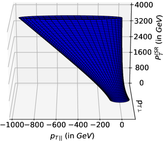
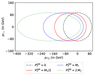
Figure 4: Illustration of the geometry of the singularity condition (41) for the mass spectrum $M_{1}=800$ GeV and $M_{0}=700$ GeV. Left panel: a 3-dimensional plot in the $(p_{T\parallel},p_{T\perp},P_{T}^{ISR})$ space of the two-dimensional singularity surface defined by eq. (41). Right panel: the boundary ellipses from Fig. 2 which were obtained at fixed values of $P_{T}^{ISR}=\{0,M_{1}/2,M_{1},2M_{1}\}$.

As a consistency check, we see that eq. (41) reduces to (35) in the limit of $P_{T}^{ISR}\to 0$. For a fixed value of $P_{T}^{ISR}$, the result (41) can be recognized as the equation of an ellipse Byckling:1971vca centered at $(-c,0)$, where $c$ is the linear eccentricity

$$c\equiv\sqrt{a^{2}-b^{2}}=\frac{M_{1}^{2}-M_{0}^{2}}{2M_{1}^{2}}\,P_{T}^{ISR},$$ (42)

while $a$ and $b$ are the semi-major and semi-minor axes, respectively:

$$a = \frac{M_{1}^{2}-M_{0}^{2}}{2M_{1}}\,\sqrt{1+\left(\frac{P_{T}^{ISR}}{M_{1}}\right)^{2}},$$ (43)

$$b = \frac{M_{1}^{2}-M_{0}^{2}}{2M_{1}}.$$ (44)

Note that the eccentricity $c$ is linearly proportional to $P_{T}^{ISR}$, thus in the case of $P_{T}^{ISR}\to 0$ considered in the previous Section 3.2.1, the ellipse (41) became the circle (35). The results (41-44) are visualized in the remaining three panels of Fig. 2, where we plot the allowed values for $\vec{p}_{1T}=(p_{T\parallel},p_{T\perp})$ for several fixed non-zero values of $P_{T}^{ISR}$: $P_{T}^{ISR}=M_{1}/2=400$ GeV (top right panel), $P_{T}^{ISR}=M_{1}=800$ GeV (bottom left panel) and $P_{T}^{ISR}=2M_{1}=1600$ GeV (bottom right panel). Since the upstream visible momentum $\vec{P}_{T}^{ISR}$ is always oriented along the positive $p_{T\parallel}$ axis, the recoil of the mother particle is in the negative $p_{T\parallel}$ direction, which explains the increasing preference for negative $p_{T\parallel}$ values as $P_{T}^{ISR}$ gets larger (see also the right panel in Fig. 4). At the same time, the (doubly) transverse components $p_{T\perp}$ are unaffected by the boost of the mother particle, and the maximal $p_{T\perp}$ value in each panel stays the same. This is also reflected in the fact that the semi-minor axis (44) of the ellipse remains constant, independent of $P_{T}^{ISR}$.

In deriving the equation of the singularity surface (41), we have achieved our main goal for this subsection. From here on, how the result (41) will be used in practice, depends on the specific purpose of the experimental analysis. If the aim is a discovery of signal events with the event topology of Fig. 1(a), one should study the distribution of events in the three-dimensional space $(p_{T\parallel},p_{T\perp},P_{T}^{ISR})$ depicted in the left panel of Fig. 4, where the signal-rich regions will be found at the locations singled out by eq. (41). If, on the other hand, the goal is to measure the mass spectrum, the singularity surface contains all the kinematic information to do that as well, and the masses $M_{0}$ and $M_{1}$ can be extracted from a parameter fit to eq. (41).

The fitting procedure will have to account for the different available statistics at different values of $P_{T}^{ISR}$. Operationally this can be accomplished as follows (following on an idea from Ref. Matchev:2009fh ). One can select a subset of events with (approximately) the same value of $P_{T}^{ISR}$, and plot them in the $\vec{p}_{1T}=(p_{T\parallel},p_{T\perp})$ plane as in Fig. 2. The signal events will exhibit an overdensity along the singularity ellipse given by (41), as also illustrated in the right panel in Fig. 4. Then, by fitting to (41), one can find the distances from the focus to the two vertices of the ellipse, i.e., the maximum value of $p_{1T}$ in the direction along $\vec{P}_{T}^{ISR}$ and in the direction opposite to $\vec{P}_{T}^{ISR}$:

$$p_{1T}^{max}(\varphi=0) = \frac{M_{1}^{2}-M_{0}^{2}}{2\left(\sqrt{M_{1}^{2}+(P_{T}^{ISR})^{2}}+P_{T}^{ISR}\right)},$$ (45)

$$p_{1T}^{max}(\varphi=\pi) = \frac{M_{1}^{2}-M_{0}^{2}}{2\left(\sqrt{M_{1}^{2}+(P_{T}^{ISR})^{2}}-P_{T}^{ISR}\right)}.$$ (46)

These two relations can be easily inverted and solved for $M_{1}$ and $M_{0}$:

$$M_{1}=2P_{T}^{ISR}\,\frac{\sqrt{p_{1T}^{max}(\varphi=\pi)p_{1T}^{max}(\varphi=0)}}{p_{1T}^{max}(\varphi=\pi)-p_{1T}^{max}(\varphi=0)},$$ (47)

$$M_{0}=2P_{T}^{ISR}\,\frac{\sqrt{p_{1T}^{max}(\varphi=\pi)p_{1T}^{max}(\varphi=0)}}{p_{1T}^{max}(\varphi=\pi)-p_{1T}^{max}(\varphi=0)}\,\sqrt{1-\frac{p_{1T}^{max}(\varphi=\pi)-p_{1T}^{max}(\varphi=0)}{P_{T}^{ISR}}}.$$ (48)

This demonstrates that the two measurements (45-46) are sufficient to determine the masses $M_{1}$ and $M_{0}$ Matchev:2009fh . The procedure can be repeated for different ranges of $P_{T}^{ISR}$, as long as there is sufficient statistics to reconstruct the singularity ellipse and from there extract the values of $p_{1T}^{max}(\varphi=0)$ and $p_{1T}^{max}(\varphi=\pi)$.

3.3 The focus point method

The discussion in the previous Sec. 3.2 revealed that for the event topology of Fig. 1(a), the location of the singularity is nicely exhibited as a two-dimensional surface in a three-dimensional space of observables $(p_{T\parallel},p_{T\perp},P_{T}^{ISR})$, as shown in the left panel in Fig. 4. But is it possible to simplify matters further, e.g., by projecting onto an observable space of even lower dimensionality, while retaining all singular features? As an extreme example, is it possible to define a single kinematic variable whose distribution will capture all of the singular behavior, over the whole surface parametrized by eq. (41)? In Section 3.2.1 we saw that for the special case of $P_{T}^{ISR}=0$ this is possible, and the relevant kinematic variable was the transverse mass $m_{T}(\tilde{M}_{0})$ (regardless of the choice of test mass $\tilde{M}_{0}$, see Fig. 3), or alternatively, the magnitude $p_{1T}$ of the transverse visible momentum. However, the subsequent discussion in Sec. 3.2.2 makes it clear that if we wish to continue using $m_{T}(\tilde{M}_{0})$ in the more general case of $P_{T}^{ISR}\neq 0$, we run into a problem — the parametrization of the singularity surface (41) involves the mass spectrum, and in particular the mass $M_{0}$ of the invisible particle. Therefore, as implied in the singularity condition (27), the transverse mass $m_{T}(\tilde{M}_{0})$ will continue to be the relevant singularity coordinate, but only for the correct choice of the test mass $\tilde{M}_{0}=M_{0}$, since only in that case the singularity surface (41) is a surface of constant $m_{T}$. If we make a wrong choice for $\tilde{M}_{0}$, which is different from the true mass $M_{0}$, the singularity surface is not a surface of constant $m_{T}$, and therefore, the singular behavior observed in the three-dimensional picture of the left panel in Fig. 4 will tend to be washed out in the one-dimensional $m_{T}(\tilde{M}_{0})$ distribution.

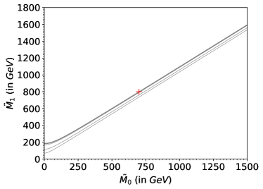
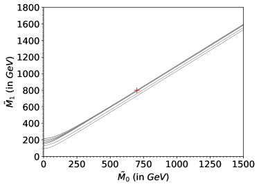
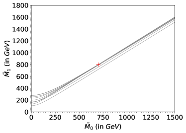
Figure 5: Focus point plots in the $(\tilde{M}_{0},\tilde{M}_{1})$ mass parameter space for different values of $P_{T}^{ISR}$: $P_{T}^{ISR}=0$ (upper left panel), $P_{T}^{ISR}=50$ GeV (upper right panel), $P_{T}^{ISR}=100$ GeV (middle left panel), $P_{T}^{ISR}=200$ GeV (middle right panel), $P_{T}^{ISR}=400$ GeV (lower left panel) and $P_{T}^{ISR}=800$ GeV (lower right panel). The plots show the solvability boundaries (49) for (the same) 10 randomly chosen events, boosted according to the corresponding $P_{T}^{ISR}$. The red “$+$” symbol marks the location of the true masses $M_{0}=700$ GeV and $M_{1}=800$ GeV.

These observations are precisely the motivation behind the focus point method for mass measurement Kim:2019prx , which can also be applied to the event topology of Fig. 1(a) considered here, with the intent of measuring the two masses $M_{1}$ and $M_{0}$. The method is illustrated in Figs. 5 and 6, where, in order to avoid overcrowding the plot, we use just a handful of events (in this case ten, chosen at random). The main idea is for each event to delineate the allowed region in the hypothesized mass parameter space $(\tilde{M}_{0},\tilde{M}_{1})$, which would lead to viable solutions for the invisible momentum $q$, given the kinematic constraints (17). It is well known that for a given test mass $\tilde{M}_{0}$, the transverse mass $m_{T}(\tilde{M}_{0})$ provides the lowest kinematically allowed value for the parent mass $M_{1}$ Gripaios:2007is ; Cheng:2008hk ; Barr:2011xt , therefore the boundary of the allowed region in our case will be given simply by the function

$$\tilde{M}_{1}=m_{T}(\tilde{M}_{0}).$$ (49)

After superimposing these kinematic boundaries from many different events as in Figs. 5 and 6, the true values of $M_{0}$ and $M_{1}$ are revealed by the location of the focus point of the kinematic boundaries Kim:2019prx .

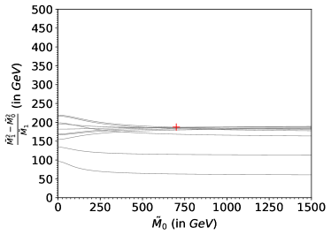
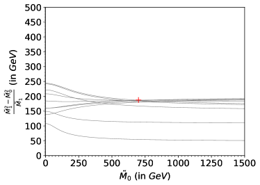
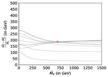
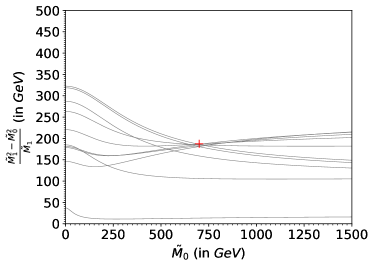
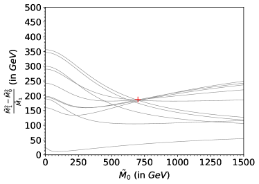
Figure 6: The same as Fig. 5, but for better visibility the quantity plotted on the $y$-xis is redefined to be $(\tilde{M}_{1}^{2}-\tilde{M}_{0}^{2})/\tilde{M}_{1}$.

This is indeed what is seen in Figs. 5 and 6 — even with the low statistics of just 10 events, a focus point emerges near the red “$+$” symbol marking the true mass point $(M_{0},M_{1})=(700\ {\rm GeV},800\ {\rm GeV})$. In an actual experimental analysis, the available statistics is expected to be much larger, perhaps as much as several orders of magnitude, thus there should be no problem observing this focus point. Note that when plotted in the $(\tilde{M}_{0},\tilde{M}_{1})$ plane as in Fig. 5, the lines tend to be parallel to each other, and their crossing is difficult to trace with the naked eye without zooming in on the relevant region near the red cross. This is why in Fig. 6 we have replotted the same data, only now replacing $\tilde{M}_{1}$ on the $y$-axis with the more relevant combination of masses $(\tilde{M}_{1}^{2}-\tilde{M}_{0}^{2})/\tilde{M}_{1}$ which enters the analytical formulas (see, e.g., eqs. (35) and (42-44)). As seen in Fig. 6, this has the benefit of removing the dependence on the overall scale $\tilde{M}_{0}$, which allows us to better concentrate on the relative differences exhibited by lines corresponding to different events.

As observed in Figs. 5 and 6 (and supported by the previous discussion in Sec. 3.2.2), the focusing effect in the event topology of Fig. 1(a) relies on the presence of some non-zero $P_{T}^{ISR}$ in the event; and the larger the $P_{T}^{ISR}$, the more pronounced the effect. In order to illustrate this, Figs. 5 and 6 depict results for several different fixed values of $P_{T}^{ISR}$: $P_{T}^{ISR}=0$ (upper left panels), $P_{T}^{ISR}=50$ GeV (upper right panels), $P_{T}^{ISR}=100$ (middle left panels), $P_{T}^{ISR}=200$ GeV (middle right panels), $P_{T}^{ISR}=400$ GeV (lower left panels) and $P_{T}^{ISR}=800$ GeV (lower right panels). Although higher values of $P_{T}^{ISR}$ would be even more beneficial to showcase our method, we limit ourselves here to these more typical values expected to come from initial state radiation (which has a steeply falling $P_{T}$ spectrum) or from decays upstream, where the typical $P_{T}$ is governed by the mass splitting of the new particles, which is likely to be around the $M_{1}$ mass scale.

Let us first discuss the upper left panels corresponding to the case of $P_{T}^{ISR}=0$ which was the subject of Sec. 3.2.1. These plots demonstrate that in the absence of any $P_{T}^{ISR}$, different values of $\tilde{M}_{0}$ are indistinguishable. In the plots, this is indicated by the fact that the lines stay roughly parallel to each other, and there are no line crossings at all. Notice that quite a few events in the figure are close to being extreme, i.e., their lines pass very close to the true mass point marked with the red cross. This is simply a consequence of the singularity condition (27) — since the ten events entering the plot were picked at random, it is more likely that they belong to the region where the event density exhibits a (singular) peak. Correspondingly, their lines appear to be “bunched up”, in the sense that their $m_{T}$ values for $\tilde{M}_{0}=M_{0}$ tend to be very similar, being so close to the true mass $M_{1}$ of the parent particle. Then, as we vary the test mass $\tilde{M}_{0}$ away from the true value $M_{0}$, the lines in the upper left panels continue to stay bunched up, confirming the presence of a singularity in the $m_{T}(\tilde{M}_{0})$ distribution for all other values of $\tilde{M}_{0}$ as well (recall Fig. 3); the exact location of the singularity as a function of $\tilde{M}_{0}$ is given by eq. (36).

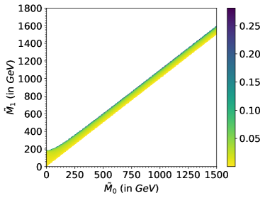
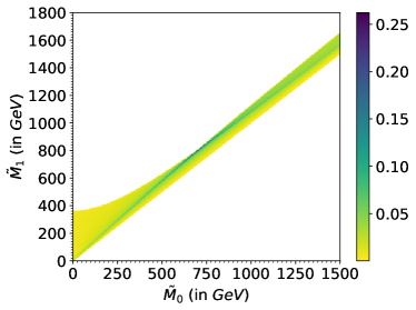
Figure 7: The heatmaps corresponding to Fig. 5, produced with a full data sample.

Fortunately, the situation changes completely in the presence of non-zero $P_{T}^{ISR}$, as illustrated in the remaining five panels in each of Figs. 5 and 6. We use the same 10 events as before, only now they have been boosted accordingly in order to generate the desired $P_{T}^{ISR}$. For illustration, let us only focus on the lower right panels with the largest $P_{T}^{ISR}=800$ GeV, where the effects are easiest to see. We observe that the lines for the near-extreme events are still bunched up in the vicinity of the red $+$ symbol, but significantly diverge away from it in the region of either very low or very high values of $\tilde{M}_{0}$ (this is especially easy to see with the parametrization used in Fig. 6). In other words, the crossing pattern of the lines has formed a focus point in the vicinity of the true mass point, and therefore, finding this focus point is a way to find the true masses Kim:2019prx . Note that the defocusing of the lines away from the true value $\tilde{M}_{0}=M_{0}$ implies that the singularity in the $m_{T}(\tilde{M}_{0})$ distribution is getting washed out when the chosen value of $\tilde{M}_{0}$ is away from the true mass $M_{0}$. This offers an alternative method for finding the true value of $M_{0}$, namely, by studying the sharpness of the singularity peak in the $m_{T}(\tilde{M}_{0})$ distribution as a function of the test value $\tilde{M}_{0}$ Kim:2019prx .

Both of those mass measurement methods are illustrated in Figs. 7 and 8, which are the analogues of Figs. 5 and 6, only this time we are using the full data sample and, following Kim:2019prx , we represent the density of curves as a heatmap where the color corresponds to the fraction of events whose lines pass through a square bin of width $2$ GeV. Fig. 7 shows the heatmaps in the $(\tilde{M}_{0},\tilde{M}_{1})$ space as in Fig. 5, while Fig. 8 uses the alternative $y$-axis reparametrization of Fig. 6.

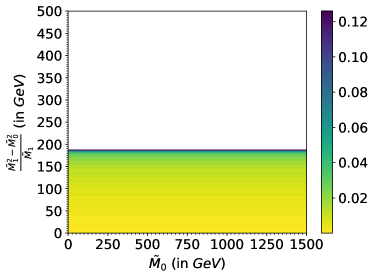
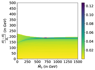
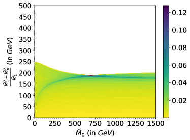
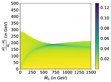
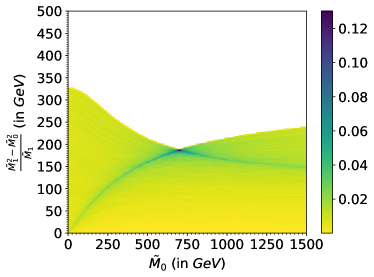
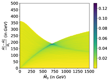
Figure 8: The same as Fig. 7, but with the $y$-axis reparametrization used in Fig. 6.

The heat maps in Figs. 7 and 8 reveal that the highest density of lines is indeed found in the vicinity of the true mass point. In the cases of non-zero $P_{T}^{ISR}$ (upper right, middle row and bottom row panels), the location of the highest density bin is unique, and this completely fixes the values of $M_{0}$ and $M_{1}$. Furthermore, when we add the statistics from all the different non-zero $P_{T}^{ISR}$ samples, the contributions to the true mass bin will add coherently, further enhancing the sharpness of the focus point. On the other hand, in the case of $P_{T}^{ISR}=0$ (upper left panels), there is a tie for the highest density bin all along the line parametrized by eq. (36); as a result, we can only determine $M_{1}$ as a function of the test mass $\tilde{M}_{0}$, but the true value of $M_{0}$ remains unknown. This is why, such events with low $P_{T}^{ISR}$ should not be used in the analysis for measuring $M_{0}$ with the focus point method.

Before concluding this section, let us discuss the connection between the focus point method presented here and the kink method for mass measurements Cho:2007qv ; Gripaios:2007is ; Barr:2007hy ; Cho:2007dh ; Matchev:2009fh . The two methods are closely related — in fact, Figs. 5-8 also nicely illustrate the kink method itself, where one instead tries to measure the maximal possible value of $m_{T}$ as a function of the test mass $\tilde{M}_{0}$. In other words, the kink method is essentially targeting the upper boundaries of the colored regions in Fig. 7, which for $P_{T}^{ISR}\neq 0$ exhibit a kink at $\tilde{M}_{0}=M_{0}$. In contrast, the focus point method is targeting the highest line density bin on the plot, and thus is designed to take full advantage of the available statistics — note that the boundaries of the colored regions in Figs. 7 and 8 are defined by just a handful of events and the extraction of the boundary (from kinematic endpoints or otherwise) is statistics-limited. On the other hand, as illustrated in Figs. 5 and 6, events which do not contribute to the boundary may still pass close to the focus point and thus usefully contribute to the focus point method. Of course, the kink occurs precisely at the location of the highest line density bin, thus the two methods in principle give the same results, as confirmed in Figs. 5-8.

4 Single decay chain, two successive two-body decays

In this section we shall discuss the event topology of Fig. 1(b) which is a cascade decay involving three new particles with masses $M_{0}$, $M_{1}$ and $M_{2}$. Correspondingly, there are three on-shell conditions

$$q^{2} = M_{0}^{2},$$ (50a)

$$(q+p_{1})^{2} = M_{1}^{2},$$ (50b)

$$(q+p_{1}+p_{2})^{2} = M_{2}^{2},$$ (50c)

which can be rewritten as

$$q^{2} = M_{0}^{2},$$ (51a)

$$2p_{1}\cdot q = M_{1}^{2}-M_{0}^{2}-m_{1}^{2},$$ (51b)

$$2p_{2}\cdot q = M_{2}^{2}-M_{1}^{2}-m_{2}^{2}-2p_{1}\cdot p_{2},$$ (51c)

At this point, we have $N_{C}=3$ constraints and $N_{q}=4$ unknowns which are the components of $q^{\mu}$. Thus in order to obtain the necessary match (9), we can do one of two things — either add an additional constraint, e.g., in the form of a measurement of one of the ${\;/\!\!\!\!\vec{P}_{T}}$ components (but not the other), or reduce the number of unknowns by going to $2+1$ dimensions, where $N_{q}=3$. Both of these options are of mostly academic interest, so for concreteness we choose the latter, which has the added benefit of somewhat simpler math (involving $3\times 3$ instead of $4\times 4$ matrices). Consequently, for the remainder of this section, we shall be working in $2+1$ dimensions, where the momenta have only transverse and no longitudinal components, i.e., $p_{i}=(e_{i},p_{ix},p_{iy})$ and $q_{i}=(\varepsilon,q_{x},q_{y})$.

The next step is to construct the Jacobian matrix (13) for the set of constraints (51):

$$D=\left(\begin{array}[]{ccc}2\varepsilon&-2q_{x}&-2q_{y}\\ 2e_{1}&-2p_{1x}&-2p_{1y}\\ 2e_{2}&-2p_{2x}&-2p_{2y}\end{array}\right).$$ (52)

The singularity condition (14) becomes

$${\rm Det}\,D=8\left|\begin{array}[]{ccc}\varepsilon&-q_{x}&-q_{y}\\ e_{1}&-p_{1x}&-p_{1y}\\ e_{2}&-p_{2x}&-p_{2y}\end{array}\right|=8\left|\begin{array}[]{ccc}\varepsilon&q_{x}&q_{y}\\ e_{1}&p_{1x}&p_{1y}\\ e_{2}&p_{2x}&p_{2y}\end{array}\right|=0.$$ (54)

Now, in order to rewrite the singularity variable appearing on the left-hand side in terms of observable momenta only, we just need to eliminate the invisible momentum components, for example, using eqs. (51). However, a more straightforward approach is to note that

$$\mathrm{Det}~{}D=0\quad\Longleftrightarrow\quad\mathrm{Det}\,D^{T}=8\left|\begin{array}[]{ccc}\varepsilon&e_{1}&e_{2}\\ -q_{x}&-p_{1x}&-p_{2x}\\ -q_{y}&-p_{1y}&-p_{2y}\end{array}\right|=0$$ (55)

and combine the last two equations as

$$64\left|\left(\begin{array}[]{ccc}\varepsilon&q_{x}&q_{y}\\ e_{1}&p_{1x}&p_{1y}\\ e_{2}&p_{2x}&p_{2y}\end{array}\right)\left(\begin{array}[]{ccc}\varepsilon&e_{1}&e_{2}\\ -q_{x}&-p_{1x}&-p_{2x}\\ -q_{y}&-p_{1y}&-p_{2y}\end{array}\right)\right|=64\left|\begin{array}[]{ccc}q^{2}&p_{1}\cdot q&p_{2}\cdot q\\ p_{1}\cdot q&p_{1}^{2}&p_{1}\cdot p_{2}\\ p_{2}\cdot q&p_{1}\cdot p_{2}&p_{2}^{2}\end{array}\right|$$ (65)

$$= 64\left|\begin{array}[]{ccc}M_{0}^{2}&~{}~{}~{}\frac{M_{1}^{2}-M_{0}^{2}-m_{1}^{2}}{2}{}{}{}&\frac{M_{2}^{2}-M_{1}^{2}-m_{2}^{2}}{2}-p_{1}\cdot p_{2}\\[5.69054pt] \frac{M_{1}^{2}-M_{0}^{2}-m_{1}^{2}}{2}&m_{1}^{2}&p_{1}\cdot p_{2}\\[5.69054pt] \frac{M_{2}^{2}-M_{1}^{2}-m_{2}^{2}}{2}-p_{1}\cdot p_{2}&p_{1}\cdot p_{2}&m_{2}^{2}\end{array}\right|=0.$$ (69)

By rewriting the singularity condition in this form, we have not only eliminated any reference to the invisible momentum components, but we also verified explicitly that the event-wise kinematic information only enters through the dot product $p_{1}\cdot p_{2}$, or equivalently, through the invariant mass $m_{12}$ of the two visible particles since the latter is related to $p_{1}\cdot p_{2}$ as

$$m_{12}^{2}\equiv(p_{1}+p_{2})^{2}=m_{1}^{2}+m_{2}^{2}+2p_{1}\cdot p_{2}.$$ (70)

Eq. (69) suggests that instead of taking the whole determinant as the singularity coordinate for this event topology, a much simpler choice would be either $p_{1}\cdot p_{2}$ or $m_{12}$, both of which have the important advantage of avoiding the necessity of an ansatz for the a priori unknown masses $M_{0}$, $M_{1}$ and $M_{2}$. For definiteness here we shall choose to work with $p_{1}\cdot p_{2}$, but $m_{12}$ will be equally good.

The locations of the singularities in the $p_{1}\cdot p_{2}$ distribution can be found from eq. (69), which leads to a quadratic equation and correspondingly two solutions. In order to simplify the formulas, let us again focus only on the case of massless visible particles, i.e., $m_{1}=m_{2}=0$, when (69) becomes

$$\left|\begin{array}[]{ccc}M_{0}^{2}&~{}~{}~{}\frac{M_{1}^{2}-M_{0}^{2}}{2}{}{}{}&\frac{M_{2}^{2}-M_{1}^{2}}{2}-p_{1}\cdot p_{2}\\[5.69054pt] \frac{M_{1}^{2}-M_{0}^{2}}{2}&0&p_{1}\cdot p_{2}\\[5.69054pt] \frac{M_{2}^{2}-M_{1}^{2}}{2}-p_{1}\cdot p_{2}&p_{1}\cdot p_{2}&0\end{array}\right|=0,$$ (71)

leading to the quadratic equation

$$(p_{1}\cdot p_{2})^{2}-\frac{(M_{2}^{2}-M_{1}^{2})(M_{1}^{2}-M_{0}^{2})}{2M_{1}^{2}}(p_{1}\cdot p_{2})=0,$$ (72)

whose solutions for $(p_{1}\cdot p_{2})$

$$(p_{1}\cdot p_{2})_{min} = 0,$$ (73a)

$$(p_{1}\cdot p_{2})_{max} = \frac{(M_{2}^{2}-M_{1}^{2})(M_{1}^{2}-M_{0}^{2})}{2M_{1}^{2}},$$ (73b)

also happen to be the two kinematic endpoints of the $p_{1}\cdot p_{2}$ distribution. The actual shape of the distribution according to pure phase space is given by

$$\frac{dN}{d(p_{1}\cdot p_{2})}=\frac{1}{\pi\sqrt{(p_{1}\cdot p_{2})\left[(p_{1}\cdot p_{2})_{max}-(p_{1}\cdot p_{2})\right]}}.$$ (74)

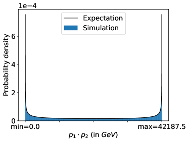
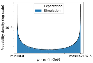
Figure 9: Distribution of the singularity variable $p_{1}\cdot p_{2}$ on a linear scale (left panel) and on a log scale (right panel). With the mass spectrum from Table 1, eq. (73) predicts the locations of the two singularities to be at $(p_{1}\cdot p_{2})_{min}=0$ and $(p_{1}\cdot p_{2})_{max}=42,187.5\ {\rm GeV}^{2}$. The black solid line shows the theoretical prediction (74) for the shape of the distribution while the histogram shows the result from the numerical simulation.

The distribution of the singularity variable $p_{1}\cdot p_{2}$ is illustrated in Fig. 9. In each panel, we plot the theoretical prediction (74) superimposed on the result from our numerical simulations. The spectrum was chosen as in Table 1: $M_{0}=700$ GeV, $M_{1}=800$ GeV and $M_{2}=1000$ GeV, which according to (73b) gives $(p_{1}\cdot p_{2})_{max}=42,187.5\ {\rm GeV}^{2}$. We see that, as expected, the distribution develops a sharp singularity at each end. These singularities are quite striking when viewed on a linear scale (as in the left panel). In order to better see the shape of the distribution in the intermediate $p_{1}\cdot p_{2}$ range, in the right panel of Fig. 9 we replotted the same data using a log scale for the y-axis.

Having derived the singularity coordinate for this case as either $p_{1}\cdot p_{2}$ or $m_{12}$ and identified the locations (73) of the two singularities, we have accomplished two of the three stated goals at the end of Sec. 2. The last goal, showcasing the focus point method of Ref. Kim:2019prx for mass measurements, is not applicable in this case, since the singularity variable is constructed out of visible momenta only, with no reference to any hypothesized mass parameters. The situation is analogous to the one already encountered in Sec. 3.2.1 — there we saw that when $P_{T}^{ISR}=0$, the singularity variable for the event topology in Fig. 1(a) can be taken to be simply the $p_{T}$ of the visible particle, and a singularity occurs for any choice of test mass as shown in the upper left panels of Figs. 5-8. The best one can do in our case here, therefore, is to obtain one constraint on the three masses $M_{0}$, $M_{1}$ and $M_{2}$ from the measurement of the upper kinematic endpoint (73b).

5 Single decay chain, three successive two-body decays

In this section we shall work out the classic SUSY decay chain of three successive two-body decays depicted in Fig. 1(c). This cascade involves four new particles with masses $M_{0}$, $M_{1}$, $M_{2}$ and $M_{3}$, which in SUSY are typically identified with the lightest neutralino, a charged slepton, the second-to-lightest neutralino, and a squark, respectively. The same decay chain also pops up in other phenomenological models of new physics such as Universal Extra Dimensions with KK-parity Appelquist:2000nn ; Rizzo:2001sd ; Cheng:2002ab , Little Higgs with $T$-parity ArkaniHamed:2002qy ; Cheng:2004yc ; Schmaltz:2005ky ; Perelstein:2005ka , etc. In any given such new physics scenario, there is a definite assignment for the spins of the new particles, however in order to stay as general as possible, we shall ignore any spin correlations (which are typically rather small anyway Athanasiou:2006ef ; Wang:2006hk ; Burns:2008cp ) and let the particles decay according to pure phase space. Unlike the toy example of the previous section, here and for the rest of the paper we shall work in $3+1$ dimensions, thus a single invisible particle with 4-momentum $q$ contributes $N_{q}=4$ unknown degrees of freedom.

We begin by listing the four on-shell conditions for the event topology of Fig. 1(c):

$$q^{2} = M_{0}^{2},$$ (75a)

$$(q+p_{1})^{2} = M_{1}^{2},$$ (75b)

$$(q+p_{1}+p_{2})^{2} = M_{2}^{2},$$ (75c)

$$(q+p_{1}+p_{2}+p_{3})^{2} = M_{3}^{2},$$ (75d)

which can be rewritten in analogy to (51) as

$$q^{2} = M_{0}^{2},$$ (76a)

$$2p_{1}\cdot q = M_{1}^{2}-M_{0}^{2}-m_{1}^{2},$$ (76b)

$$2p_{2}\cdot q = M_{2}^{2}-M_{1}^{2}-m_{2}^{2}-2p_{1}\cdot p_{2},$$ (76c)

$$2p_{3}\cdot q = M_{3}^{2}-M_{2}^{2}-m_{3}^{2}-2p_{1}\cdot p_{3}-2p_{2}\cdot p_{3}.$$ (76d)

Since we already have $N_{C}=4$ constraints for $N_{q}=4$ unknowns, the condition (9) is already met and we can proceed with the derivation of the Jacobian matrix (13)

$$D=\left(\begin{array}[]{cccc}2\varepsilon&-2q_{x}&-2q_{y}&-2q_{z}\\ 2e_{1}&-2p_{1x}&-2p_{1y}&-2p_{1z}\\ 2e_{2}&-2p_{2x}&-2p_{2y}&-2p_{2z}\\ 2e_{3}&-2p_{3x}&-2p_{3y}&-2p_{3z}\end{array}\right)$$ (77)

and the singularity condition (14)

$${\rm Det}\,D=16\left|\begin{array}[]{cccc}\varepsilon&-q_{x}&-q_{y}&-q_{z}\\ e_{1}&-p_{1x}&-p_{1y}&-p_{1z}\\ e_{2}&-p_{2x}&-p_{2y}&-p_{2z}\\ e_{3}&-p_{3x}&-p_{3y}&-p_{3z}\end{array}\right|=0.$$ (79)

In order to obtain a singularity variable in terms of the visible momenta only, we need to eliminate the invisible momentum components with the help of (76). However, the same task is more easily accomplished with the determinant trick used in the previous section: after noting that

$$\mathrm{Det}~{}D=0\quad\Longleftrightarrow\quad{\rm Det}\,D^{T}=16\left|\begin{array}[]{cccc}\varepsilon&e_{1}&e_{2}&e_{3}\\ -q_{x}&-p_{1x}&-p_{2x}&-p_{3x}\\ -q_{y}&-p_{1y}&-p_{2y}&-p_{3y}\\ -q_{z}&-p_{1z}&-p_{2z}&-p_{3z}\end{array}\right|=0,$$ (80)

we can combine the last two equations into

$${\rm Det}\,D=0\Longleftrightarrow{\rm Det}\left(D\eta D^{T}\right)=256\left|\begin{array}[]{cccc}q^{2}&~{}p_{1}\cdot q{}&~{}p_{2}\cdot q{}&~{}p_{3}\cdot q{}\\[2.84526pt] p_{1}\cdot q&p_{1}^{2}&p_{1}\cdot p_{2}&p_{1}\cdot p_{3}\\[2.84526pt] p_{2}\cdot q&p_{1}\cdot p_{2}&p_{2}^{2}&p_{2}\cdot p_{3}\\[2.84526pt] p_{3}\cdot q&p_{1}\cdot p_{3}&p_{2}\cdot p_{3}&p_{3}^{2}\end{array}\right|=0,$$ (81)

with $\eta$ being the Minkowski $4\times 4$ metric

$$\eta={\rm diag}(1,-1,-1,-1).$$ (82)

With the use of (76), the dot products of momenta appearing in (81) can now easily be traded for the relevant masses. Once again, the result simplifies significantly in the case of massless visible particles, i.e., $p_{1}^{2}=p_{2}^{2}=p_{3}^{2}=0$, when (81) reduces to

$$-256\,\left|\begin{array}[]{cccc}M_{0}^{2}&~{}\frac{M_{1}^{2}-M_{0}^{2}}{2}{}&~{}\frac{M_{2}^{2}-M_{1}^{2}-m_{12}^{2}}{2}{}&~{}\frac{M_{3}^{2}-M_{2}^{2}-m_{23}^{2}-m_{13}^{2}}{2}{}\\[5.69054pt] \frac{M_{1}^{2}-M_{0}^{2}}{2}&0&\frac{m_{12}^{2}}{2}&\frac{m_{13}^{2}}{2}\\[5.69054pt] \frac{M_{2}^{2}-M_{1}^{2}-m_{12}^{2}}{2}&\frac{m_{12}^{2}}{2}&0&\frac{m_{23}^{2}}{2}\\[5.69054pt] \frac{M_{3}^{2}-M_{2}^{2}-m_{23}^{2}-m_{13}^{2}}{2}&\frac{m_{13}^{2}}{2}&\frac{m_{23}^{2}}{2}&0\end{array}\right|=0,$$ (83)

where $m_{ij}$ are the pair-wise invariant masses of the three (massless) visible particles:

$$m_{ij}^{2}\equiv(p_{i}+p_{j})^{2}=2p_{i}\cdot p_{j}.$$ (84)

Up to the numerical prefactor of 256, the left-hand side of (83) is precisely the $\Delta_{4}$ variable introduced in Byckling:1971vca ; Agrawal:2013uka . We have thus rederived from first principles the well-known fact that $\Delta_{4}$ is the relevant singularity variable for the event topology of Fig. 1(c), and that the locations of singularities are those where $\Delta_{4}=0$. Eq. (83) also confirms that the relevant observable phase space is only three-dimensional, and can be conveniently parametrized with the pair-wise invariant masses as

$$\left\{m_{12}^{2},m_{23}^{2},m_{13}^{2}\right\}.$$ (85)

Given the ubiquity of the decay chain of Fig. 1(c) in SUSY and elsewhere, it is not surprising that the properties of the allowed region within this invariant mass phase space have been extensively studied in the literature. Therefore, rather than reproducing previously published work, here we shall only state the results most relevant to the current discussion, and for further details we refer the reader to the corresponding literature.

• The shape of the allowed region in phase space. The allowed region in the visible invariant mass space (85) is compact, and is bounded by the (closed) two-dimensional surface defined by eq. (83). Three-dimensional plots of the allowed region can be found in Fig. 1 of Costanzo:2009mq , Fig. 9 of Kim:2015bnd and on pages 568-572 of the TASI lectures Lester:2013aaa .

• Density enhancement on the boundary. The phase space singularities occur on the two-dimensional boundary of the allowed region, i.e., the condition $\Delta_{4}=0$ (which is equivalent to (83)) defines both the boundary of the allowed region as well as the singularity locations Agrawal:2013uka . Since the allowed region is three-dimensional, it is difficult to visualize this enhancement unless one looks at two-dimensional slices through the allowed region — such plots can be found in Fig. 8 of Debnath:2016mwb and Fig. 12 of Debnath:2016gwz .

• The shape of the one-dimensional distribution of the singularity variable. The differential distribution of $\Delta_{4}$ is known analytically. In terms of the unit-normalized variable $q\equiv\Delta_{4}/\Delta_{4}^{max}$ it is given by Debnath:2016mwb

  $$\frac{dN}{dq}=\frac{\arcsin(\sqrt{1-q})}{2\sqrt{q}}.$$ (86)

  The sharp peak at $\Delta_{4}=0$ can be used for discovering such new physics signal over the smooth SM background, as discussed in Debnath:2018azt .

• Mass measurements and the focus point method. Since computing the singularity variable $\Delta_{4}$ requires an ansatz for the mass spectrum, the focus point method for mass measurements Kim:2019prx is in principle applicable, and one would be looking for a peak in the 4-dimensional parameter space of $\{M_{0},M_{1},M_{2},M_{3}\}$. However, the relevant observable parameter space (85), being only three-dimensional, is already simple enough so that in practice it may be easier to just perform a four-parameter fit to the boundary of the allowed region, as demonstrated in Debnath:2016gwz .

6 Two decay chains, each with one two-body decay

In this section we shall simultaneously address the two event topologies shown in Figs. 1(d) and 1(e). The latter is known as the “antler” topology Han:2009ss and has been previously discussed in the context of both hadron colliders Baumgart:2006pa ; Barr:2009mx ; Han:2009ss ; Choi:2009hn ; Barr:2011he ; Park:2011uz ; Barr:2011ux ; Edelhauser:2012xb ; DeRujula:2012ns ; Han:2012nm ; Konar:2015hea and lepton colliders Christensen:2014yya ; Choi:2015afa . At the same time, the diagram of Fig. 1(d) is extremely common, and may represent many processes, including but not limited to $W$-pair production in the SM, squark or slepton production in SUSY, etc. This diagram also has been extensively discussed in the literature — at lepton colliders Feng:1993sd ; HarlandLang:2012gn ; Xiang:2016jni , and especially at hadron colliders, where it offers a formidable challenge, despite its apparent simplicity (for reviews, see Barr:2010zj ; Matchev:2019sqa ). In fact, it was precisely the diagram of Fig. 1(d) which initially motivated a large number of now popular kinematic variables and techniques, including the Cambridge $M_{T2}$ variable Lester:1999tx ; Barr:2003rg and its variants Burns:2008va ; Barr:2009jv ; Konar:2009wn ; Konar:2009qr , the contransverse mass $M_{CT}$ Tovey:2008ui , the $M_{CT2}$ variable Cho:2009ve ; Cho:2010vz , the MAOS method Cho:2008tj ; Guadagnoli:2013xia , and many others.

Given the similarities in the diagrams of Figs. 1(d) and 1(e), in this section we shall discuss them in one go by assuming the 4-momentum vector of the initial state ${\cal P}=({\cal P}_{0},\vec{\cal P})$ to be fixed. This is certainly true at lepton colliders, where the kinematics of the initial state is completely known: ${\cal P}=(E_{CM},0,0,0)$, where $E_{CM}$ is the beam CM energy, which in the case of the antler diagram of Fig. 1(e) can be tuned to be equal to the mass $M_{2}$ of the intermediate resonance, so that ${\cal P}$ becomes ${\cal P}=(M_{2},0,0,0)$. At hadron colliders, we will primarily focus on the antler diagram of Fig. 1(e), for which the 4-momentum of the initial state can be written as ${\cal P}=(\sqrt{M_{2}^{2}+{\cal P}_{z}^{2}},0,0,{\cal P}_{z})$, since in general the resonance of mass $M_{2}$ will be produced with some non-zero longitudinal momentum ${\cal P}_{z}$, whose size will be governed by the value of $M_{2}$ and the parton distribution functions (pdfs) of the initial state partons. For completeness, we shall initially retain ${\cal P}_{z}$ in our formulas, but in the end, following DeRujula:2012ns , we shall take the “gluon collider” approximation ${\cal P}_{z}\approx 0$, which can be justified in cases where the pdfs of the initial state partons are the same (or similar) and are fast-falling functions, e.g., as in the SM process $H\to W^{+}W^{-}$ DeRujula:2012ns .

6.1 Derivation of a singularity coordinate

The event topologies of Figs. 1(d) and 1(e) have the following constraints in common:

$$q^{2} = M_{0}^{2},$$ (87a)

$$Q^{2} = M_{0}^{2},$$ (87b)

$$(q+p_{1})^{2} = M_{1}^{2},$$ (87c)

$$(Q+P_{1})^{2} = M_{1}^{2},$$ (87d)

$$q_{x}+Q_{x} = {\;/\!\!\!\!P_{x}}=-p_{1x}-P_{1x},$$ (87e)

$$q_{y}+Q_{y} = {\;/\!\!\!\!P_{y}}=-p_{1y}-P_{1y},$$ (87f)

where in the last two equations we have assumed that there is no $P_{T}^{ISR}$ accompanying our event topology, hence ${\;/\!\!\!\!\vec{P}_{T}}=-\vec{p}_{1T}-\vec{P}_{1T}$.

Since we are treating the initial state kinematics as fixed, we can add two more relations representing energy conservation and longitudinal momentum conservation, respectively

$$\epsilon+{\cal E} = {\cal P}_{0}-e_{1}-E_{1},$$ (88a)

$$q_{z}+Q_{z} = {\cal P}_{z}-p_{1z}-P_{1z},$$ (88b)

with some fixed ${\cal P}_{0}$ and ${\cal P}_{z}$ as discussed above. Eqs. (87e-88b) can now be used to eliminate the 4-momentum $Q$ as

$$Q={\cal P}-p_{1}-P_{1}-q.$$ (89)

Substituting this into eqs. (87b) and (87d), and again limiting ourselves for simplicity to the case of massless visible particles, $p_{1}^{2}=P_{1}^{2}=0$, we can rewrite the four remaining constraints (87a-87d) as

$$q^{2} = M_{0}^{2},$$ (90a)

$$2\,p_{1}\cdot q = M_{1}^{2}-M_{0}^{2},$$ (90b)

$$2\,P_{1}\cdot q = -M_{1}^{2}+M_{0}^{2}+2({\cal P}-p_{1})\cdot P_{1},$$ (90c)

$$2\,{\cal P}\cdot q = {\cal P}^{2}-2{\cal P}\cdot p_{1}.$$ (90d)

From here we can compute the Jacobian matrix (13)

$$D=\left(\begin{array}[]{cccc}2\varepsilon&-2q_{x}&-2q_{y}&-2q_{z}\\ 2e_{1}&-2p_{1x}&-2p_{1y}&-2p_{1z}\\ 2E_{1}&-2P_{1x}&-2P_{1y}&-2P_{1z}\\ 2{\cal P}_{0}&0&0&-2{\cal P}_{z}\end{array}\right)$$ (91)

and the singularity condition then reads

$${\rm Det}\,D=0\Longleftrightarrow{\rm Det}\,(D\eta D^{T})=0,$$ (92)

which implies

$$\left|\begin{array}[]{cccc}~{}2q^{2}{}&~{}~{}2p_{1}\cdot q{}{}&~{}~{}2P_{1}\cdot q{}{}&~{}~{}2{\cal P}\cdot q{}{}\\[2.84526pt] 2p_{1}\cdot q&0&2p_{1}\cdot P_{1}&2{\cal P}\cdot p_{1}\\[2.84526pt] 2P_{1}\cdot q&2p_{1}\cdot P_{1}&0&2{\cal P}\cdot P_{1}\\[2.84526pt] 2{\cal P}\cdot q&2{\cal P}\cdot p_{1}&2{\cal P}\cdot P_{1}&2{\cal P}^{2}\end{array}\right|=0.$$ (93)

Using (90) to eliminate $q$, after a couple of row and column manipulations, this simplifies to

$$\Delta_{antler}\equiv\left|\begin{array}[]{cccc}2M_{1}^{2}&~{}M_{1}^{2}-M_{0}^{2}{}&~{}-M_{1}^{2}+M_{0}^{2}+2{\cal P}\cdot P_{1}{}&{\cal P}^{2}\\[5.69054pt] M_{1}^{2}-M_{0}^{2}&0&2p_{1}\cdot P_{1}&2{\cal P}\cdot p_{1}\\[5.69054pt] -M_{1}^{2}+M_{0}^{2}+2{\cal P}\cdot P_{1}&2p_{1}\cdot P_{1}&0&2{\cal P}\cdot P_{1}\\[5.69054pt] {\cal P}^{2}&2{\cal P}\cdot p_{1}&2{\cal P}\cdot P_{1}&2{\cal P}^{2}\end{array}\right|=0,$$ (94)

where the left-hand side is precisely the desired singularity variable $\Delta_{antler}$ for the case of Figs. 1(d) and 1(e). Eq. (94) indicates that the relevant phase space of kinematic observables is three-dimensional and can be parametrized, e.g., as

$$\left\{{\cal P}\cdot p_{1},~{}{\cal P}\cdot P_{1},~{}p_{1}\cdot P_{1}\right\}.$$ (95)

Just like the singularity variable $\Delta_{4}$ from Sec. 5, the singularity variable $\Delta_{antler}$ depends not only on the phase space (95), but also requires an ansatz $\tilde{M}_{1}$ and $\tilde{M}_{0}$ for the two mass parameters, i.e., $\Delta_{antler}(\tilde{M}_{1},\tilde{M}_{0})$. If the ansatz is correct ($\tilde{M}_{1}=M_{1}$ and $\tilde{M}_{0}=M_{0}$), then the singularity condition (94) guarantees that the distribution of $\Delta_{antler}$ exhibits a singularity peak at

$$\Delta_{antler}(M_{1},M_{0})=0.$$ (96)

This is demonstrated in the left panel of Fig. 10, which shows the one-dimensional unit-normalized distribution of $\Delta_{antler}(M_{1},M_{0})$ at a lepton collider with $E_{CM}(=M_{2})=3000$ GeV, and with the mass spectrum from Table 1, $M_{1}=800$ GeV and $M_{0}=700$ GeV. As expected, there is a sharp peak at $\Delta_{antler}=0$. We also note that with our conventions the values of $\Delta_{antler}$ are negative — this can be traced back to eq. (92) and the fact that with the correct choice of mass parameters $D$ is guaranteed to be real and thus ${\rm Det}\,DD^{T}>0$, while ${\rm Det}\,\eta=-1$.

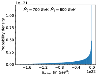
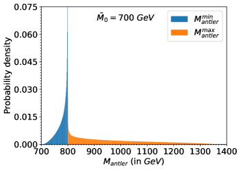
Figure 10: One-dimensional distributions of the singularity variables $\Delta_{antler}(M_{1},M_{0})$ (left panel) and $M_{antler}(M_{0})$ (right panel). In each plot, we use the true mass(es) for the respective mass parameter ansatz. Events were generated with the mass spectrum from Fig. 1 at a lepton collider with ${\cal P}=(M_{2},0,0,0)$ and $M_{2}=3000$ GeV. In the right panel, the orange (blue) histogram corresponds to the larger solution $M_{antler}^{max}$ (smaller solution $M_{antler}^{min}$) of eq. (97).

However, the mass spectrum may not always be known a priori, thus one would like to reduce the number of mass ansatze as much as possible. To this end, we can follow the idea of the transverse mass $m_{T}$ from Sec. 3, which takes only $\tilde{M}_{0}$ as an input and then uses the corresponding singularity condition (22) to define the singularity variable. In our case, we can use (96) to define implicitly an alternative singularity variable $M_{antler}(\tilde{M}_{0})$ as the solution to the equation

$$\Delta_{antler}(M_{antler},\tilde{M}_{0})=0.$$ (97)

The distribution of $M_{antler}$ for $\tilde{M}_{0}=M_{0}$ is shown in the right panel of Fig. 10. Notice that the defining equation (97) leads to a quadratic equation for $M_{antler}$ and therefore to two possible solutions, both of which are entered in the plot. The larger of the two solutions, which we label $M_{antler}^{max}$, comprises the orange histogram, while the smaller one, labelled $M_{antler}^{min}$, makes up the blue histogram, and the two histograms are individually normalized to $1$. As expected, the right panel of Fig. 10 exhibits the presence of a sharp peak at the correct mass of the parent particle, $M_{1}=800$ GeV. It is interesting to note that both solutions $M_{antler}^{min}$ and $M_{antler}^{max}$ are contributing to the singularity — from below and from above, respectively. Another noteworthy feature of the plot is that the orange and blue histograms do not overlap at all — in fact, they meet at the true value of the mass $M_{1}=800$ GeV (which is also the location of the singularity peak). This can be seen even more clearly in Fig. 11, which shows the two-dimensional distribution of events as a heatmap in the plane of $(M_{antler}^{max},M_{antler}^{min})$.

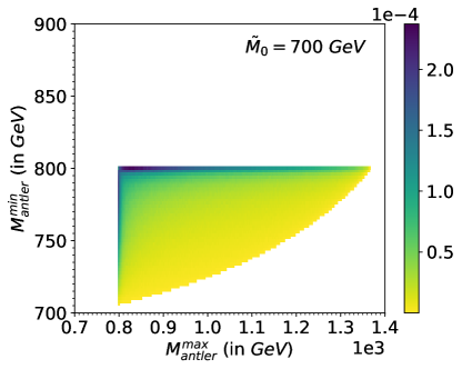
Figure 11: A heatmap of the two-dimensional distribution of events versus the two solutions for the singularity variable $M_{antler}$, namely $M_{antler}^{max}$ (plotted on the $x$-axis) and $M_{antler}^{min}$ (plotted on the $y$-axis).

The heatmap in Fig. 11 reveals an overdensity of events at both $M_{antler}^{min}=M_{1}$ (the horizontal blue-shaded band) and $M_{antler}^{max}=M_{1}$ (the vertical blue-shaded band). This confirms that both solutions for $M_{antler}$ play a role in forming the singularity peak observed in the right panel of Fig. 10. Note also the absence of any events with $M_{antler}^{min}>M_{1}$ and $M_{antler}^{max}<M_{1}$, which implies that the following hierarchy is always true:

$$M_{antler}^{min}\leq M_{1}\leq M_{antler}^{max}.$$ (98)

In other words, the true parent mass $M_{1}$ is always located between the two found solutions for $M_{antler}$, and furthermore, $M_{1}$ is the upper kinematic endpoint of $M_{antler}^{min}$ (the blue histogram in the right panel of Fig. 10) and at the same time it is also the lower kinematic endpoint of $M_{antler}^{max}$ (the orange histogram in the right panel of Fig. 10). This can be understood as follows. The two solutions for $M_{antler}$ obtained from the singularity condition (97) represent the two values for the trial mass $\tilde{M}_{1}$ where the number of solutions for the invisible momentum $q$ changes Kim:2019prx , in this case between 0 and 2. Since the true mass $M_{1}$ will always give valid solutions for $q$, it belongs to the allowed interval for $\tilde{M}_{1}$ with 2 solutions, which is sandwiched between the two disallowed regions with 0 solutions.

In summary, the discussion in this subsection (and Fig. 10 in particular) shows that both $\Delta_{antler}$ and $M_{antler}$ are valid singularity variables, albeit the latter has the added advantages of having a clear physical meaning and being of mass dimension 1 only.

6.2 The phase space geometry of the singularity condition

Having derived the singularity variables for the event topologies of Figs. 1(d) and 1(e), we can now discuss the geometry of the singularity surface in the relevant observable phase space. The latter can be parametrized as in (95), but the equation of the singularity surface (94) can be written more compactly if we use an alternative set of observables

$${\cal X} = 2({\cal P}\cdot p_{1}+{\cal P}\cdot P_{1}),$$ (99a)

$${\cal Y} = 2({\cal P}\cdot p_{1}-{\cal P}\cdot P_{1}),$$ (99b)

$${\cal Z} = \frac{4({\cal P}\cdot p_{1})({\cal P}\cdot P_{1})}{{\cal P}^{2}}-2(p_{1}\cdot P_{1})$$ (99c)

which reduces (94) to the constraint

$$\frac{\left[{\cal X}-{\cal P}^{2}\left(1-\frac{M_{0}^{2}}{M_{1}^{2}}\right)\right]^{2}}{\left(1-\frac{M_{0}^{2}}{M_{1}^{2}}\right)^{2}-\frac{\cal Z}{M_{1}^{2}}}+\frac{{\cal Y}^{2}}{\frac{\cal Z}{M_{1}^{2}}}={\cal P}^{2}\left({\cal P}^{2}-4M_{1}^{2}\right).$$ (100)

This equation describes a closed surface whose cross-sections at fixed ${\cal Z}$ are ellipses in the $({\cal X},{\cal Y})$ plane. As discussed earlier, for illustration purposes, we shall now fix the momentum of the initial state as ${\cal P}=(M_{2},0,0,0)$, which can be viewed as a lepton collider running at a CM energy $E_{CM}=M_{2}=3000$ GeV and producing either one of the diagrams in Figs. 1(d) and 1(e), or as a hadron collider producing the antler topology, where one neglects the longitudinal momentum of the heavy $s$-channel resonance DeRujula:2012ns . In that limit, the variables (99) become

$${\cal X} = 2M_{2}(e_{1}+E_{1}),$$ (101a)

$${\cal Y} = 2M_{2}(e_{1}-E_{1}),$$ (101b)

$${\cal Z} = 2(e_{1}E_{1}+\vec{p}_{1}\cdot\vec{P}_{1})\equiv M_{C}^{2}.$$ (101c)

In the last line we recognize the quantity $M_{C}$ introduced in Tovey:2008ui , which is invariant under contra-linear (back-to-back) boosts. We can use this boost invariance to bring the two intermediate particles of mass $M_{1}$ to their corresponding rest frames (along with their decay products), which then allows us to express the quantity $M_{C}$ as

$$M_{C}^{2}\equiv\frac{M_{1}^{2}}{2}\left(1-\frac{M_{0}^{2}}{M_{1}^{2}}\right)^{2}(1+\cos\theta^{\ast}),$$ (102)

where $\theta^{\ast}$ is the angle between $\vec{p}_{1}$ and $\vec{P}_{1}$ after the respective boosts. With the help of (101) and (102), the equation of the singularity surface (100) becomes

$$\frac{\left[(e_{1}+E_{1})-\frac{M_{2}}{2}\left(1-\frac{M_{0}^{2}}{M_{1}^{2}}\right)\right]^{2}}{\sin^{2}\frac{\theta^{\ast}}{2}}+\frac{(e_{1}-E_{1})^{2}}{\cos^{2}\frac{\theta^{\ast}}{2}}=\frac{M_{2}^{2}}{4}\left(1-\frac{M_{0}^{2}}{M_{1}^{2}}\right)^{2}\left(1-\frac{4M_{1}^{2}}{M_{2}^{2}}\right).$$ (103)

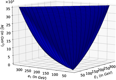
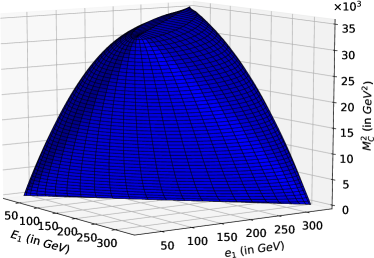
Figure 12: Two different views of the singularity surface defined by eqs. (100) and (103). The observable phase space is parametrized as $(e_{1},E_{1},M_{C}^{2})$.

The singularity surface defined by this equation is pictorially illustrated in Figs. 12 and 13. Fig. 12 is analogous to the plot in the left panel of Fig. 4 from Sec. 3.2.2, where the space of relevant observables was three-dimensional as well. In Fig. 12, we show two different views of the singularity surface when, as suggested by eq. (101), the observable phase space is parametrized as $(e_{1},E_{1},M_{C}^{2})$.

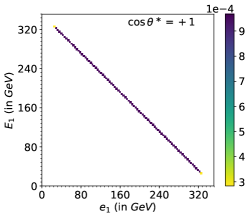
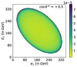
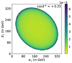
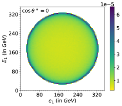
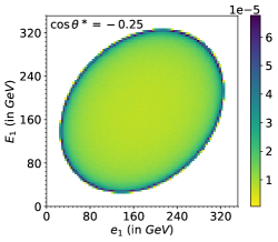
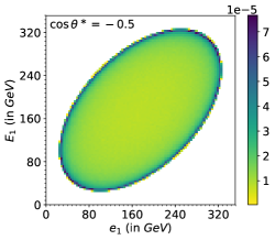
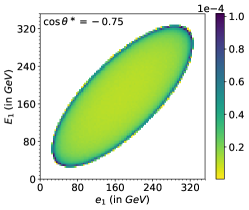
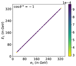
Figure 13: Allowed values for the energies $e_{1}$ and $E_{1}$ of the two visible particles for different fixed values of $M_{C}$, or equivalently, $\cos\theta^{\ast}$. The plots from top to bottom are for fixed $\cos\theta^{\ast}=\{+1.0,+0.75,+0.50,+0.25,0,-0.25,-0.50,-0.75,-1.0\}$.

Fig. 13, on the other hand, shows a series of plots in analogy to Fig. 2. Each individual panel depicts the allowed range of values for the energies $e_{1}$ and $E_{1}$ of the two visible particles for a given fixed value of $M_{C}$, or equivalently, for a fixed value of $\cos\theta^{\ast}$, since the two are related by eq. (102). For this figure we prefer to work with $\cos\theta^{\ast}$ (and equally spaced fixed values for it) since the distribution in $\cos\theta^{\ast}$ is uniform, thus each panel in Fig. 13 has the same total number of events. The event number density in the $(e_{1},E_{1})$ plane is indicated by the color bar. We see that, as expected, the events tend to cluster on the singularity boundary, whose shape is an ellipse of varying eccentricity depending on the value of $\cos\theta^{\ast}$. The distortion in the shape of the elliptical boundary can be easily tracked and understood with the help of eq. (103). Consider, for example, the case of $\cos\theta^{\ast}=+1$ shown in the upper left panel of Fig. 13. This implies that $\theta^{\ast}=0$ and the first term in the left hand side of (103) dominates, which in turn implies the linear relation $e_{1}+E_{1}=\frac{M_{2}}{2}\left(1-\frac{M_{0}^{2}}{M_{1}^{2}}\right)=351.6$ GeV seen in the plot. As the value of $\cos\theta^{\ast}$ decreases, the elliptical boundary becomes less eccentric, and for $\cos\theta^{\ast}=0$, i.e., $\theta^{\ast}=\frac{\pi}{4}$, it eventually becomes a circle, as seen in the middle plot of the middle row. As the value of $\cos\theta^{\ast}$ decreases further, the ellipse begins to stretch along the orthogonal $e_{1}=E_{1}$ direction, and for $\cos\theta^{\ast}=-1$ it simply becomes the line $e_{1}=E_{1}$.

6.3 The focus point method

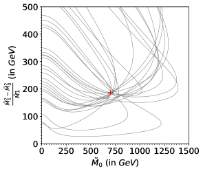
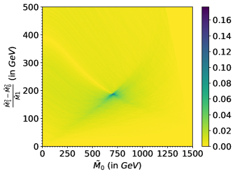
Figure 14: Focus point plots in the $(\tilde{M}_{0},(\tilde{M}_{1}^{2}-\tilde{M}_{0}^{2})/\tilde{M}_{1})$ plane for the event topologies of Figs. 1(d) and 1(e) with fixed ${\cal P}=(M_{2},0,0,0)$ and $M_{2}=3000$ GeV. We use 20 randomly chosen events in the left panel, in which the red “$+$” symbol marks the location of the true masses, and 10,000 events to produce the heatmap in the right panel, where the color indicates the fraction of events whose solvability boundaries pass through a given $2\times 2$ GeV bin.

Before concluding this section, we shall demonstrate that the focus point method of Ref. Kim:2019prx applies to the event topologies of Figs. 1(d) and 1(e) as well. The point is that the singularity variable $\Delta_{antler}$ derived in Sec. 6.1 requires a mass ansatz $\tilde{M}_{1}$ and $\tilde{M}_{0}$ as input. The need for such mass ansatze was once considered undesirable, but, as more recent studies have shown, it is precisely the dependence on the test masses that opens the door to new methods for extracting useful information about the mass spectrum, case in point being the kink method for measuring $M_{0}$ Cho:2007qv ; Gripaios:2007is ; Barr:2007hy ; Cho:2007dh ; Matchev:2009fh .

In our case, the ansatz for $\tilde{M}_{1}$ and $\tilde{M}_{0}$ is needed to provide the needed number of kinematic constraints, which would allow us to solve for the invisible momenta. However, not all choices of $\tilde{M}_{1}$ and $\tilde{M}_{0}$ will lead to real solutions. Each event will thus delineate a viable region in the $(\tilde{M}_{0},\tilde{M}_{1})$ mass parameter space. The idea of the focus point method is to superimpose the boundaries of the allowed regions selected by different events, as illustrated in the left panel of Fig. 14. The plot shows the solvability boundaries defined by

$$\Delta_{antler}(\tilde{M}_{1},\tilde{M}_{0})=0$$ (104)

for 20 randomly chosen events, where for better visualization, we have rescaled the $y$-axis as was previously done in Figs. 6 and 8. We see that even with just a handful of events, the solvability boundary curves tend to focus near the true mass point, marked with the red “$+$” symbol. With a lot more statistics, we obtain the heatmap shown in the right panel of Fig. 14 (contrast to the analogous heatmaps seen in Fig. 8). The heatmap clearly identifies the singularity peak which is situated at the true values of the masses, thus establishing the viability of the method.

7 Two decay chains, each with two successive two-body decays

For completeness, in this section we shall review the final event topology from Fig. 1, namely, the dilepton $t\bar{t}$ event topology in Fig. 1(f), which was also the one used in Ref. Kim:2019prx to introduce and illustrate the idea of the focus point method for mass measurements. Correspondingly, we shall not repeat the analysis of Ref. Kim:2019prx here, and simply refer the readers interested in mass measurements aspects to that paper. Here we shall focus more narrowly on the derivation of a singularity coordinate for that case, following the general method outlined in Sec. 2.2 and illustrated with the examples from the previous sections.

Let us begin by listing the kinematic constraints for the event topology from Fig. 1(f):

$$q^{2} = M_{0}^{2},$$ (105a)

$$Q^{2} = M_{0}^{2},$$ (105b)

$$(q+p_{1})^{2} = M_{1}^{2},$$ (105c)

$$(Q+P_{1})^{2} = M_{1}^{2},$$ (105d)

$$(q+p_{1}+p_{2})^{2} = M_{2}^{2},$$ (105e)

$$(Q+P_{1}+P_{2})^{2} = M_{2}^{2},$$ (105f)

$$q_{x}+Q_{x} = {\;/\!\!\!\!P_{x}},$$ (105g)

$$q_{y}+Q_{y} = {\;/\!\!\!\!P_{y}},$$ (105h)

which can be rewritten as

$$q^{2} = M_{0}^{2},$$ (106a)

$$2\,p_{1}\cdot q = M_{1}^{2}-M_{0}^{2}-m_{1}^{2},$$ (106b)

$$2\,p_{2}\cdot q = M_{2}^{2}-M_{1}^{2}-m_{2}^{2}-2p_{1}\cdot p_{2},$$ (106c)

$$Q^{2} = M_{0}^{2},$$ (106d)

$$2\,P_{1}\cdot Q = M_{1}^{2}-M_{0}^{2}-m_{1}^{2},$$ (106e)

$$2\,P_{2}\cdot Q = M_{2}^{2}-M_{1}^{2}-m_{2}^{2}-2P_{1}\cdot P_{2},$$ (106f)

$$q_{x}+Q_{x} = {\;/\!\!\!\!P_{x}},$$ (106g)

$$q_{y}+Q_{y} = {\;/\!\!\!\!P_{y}}.$$ (106h)

Within the dilepton $t\bar{t}$ example of the SM, the three masses are known: $M_{2}$ is the mass of the top quark, $M_{1}$ is the mass of the $W$ boson and $M_{0}$ is the neutrino mass. However, the event topology of Fig. 1(f) is relevant not only for top physics, but also for new physics searches, where the masses $M_{2}$, $M_{1}$ and $M_{0}$ may correspond to new BSM particles and thus may not be known a priori, again forcing us to use an ansatz $\{\tilde{M}_{2},\tilde{M}_{1},\tilde{M}_{0}\}$ for the mass spectrum. Either way, eqs. (106) provide 8 constraints for the 8 unknown components of the invisible momenta $q$ and $Q$, and one can thus solve for $q$ and $Q$ in terms of the mass ansatz by standard means Sonnenschein:2005ed ; Sonnenschein:2006ud ; Betchart:2013nba , obtaining

$$\tilde{q} = q(\tilde{M}_{2},\tilde{M}_{1},\tilde{M}_{0}),$$ (107a)

$$\tilde{Q} = Q(\tilde{M}_{2},\tilde{M}_{1},\tilde{M}_{0}).$$ (107b)

The Jacobian matrix (13) for the system (106) is

$$D_{t\bar{t}}(\tilde{M}_{2},\tilde{M}_{1},\tilde{M}_{0})\equiv\left(\begin{array}[]{cccccccc}2\tilde{\varepsilon}&-2\tilde{q}_{x}&-2\tilde{q}_{y}&-2\tilde{q}_{z}&0&0&0&0\\ 2e_{1}&-2p_{1x}&-2p_{1y}&-2p_{1z}&0&0&0&0\\ 2e_{2}&-2p_{2x}&-2p_{2y}&-2p_{2z}&0&0&0&0\\ 0&0&0&0&2\tilde{\cal E}&-2\tilde{Q}_{x}&-2\tilde{Q}_{y}&-2\tilde{Q}_{z}\\ 0&0&0&0&2E_{1}&-2P_{1x}&-2P_{1y}&-2P_{1z}\\ 0&0&0&0&2E_{2}&-2P_{2x}&-2P_{2y}&-2P_{2z}\\ 0&1&0&0&0&1&0&0\\ 0&0&1&0&0&0&1&0\end{array}\right),$$ (108)

where the dependence on the mass ansatz enters through the solutions for the invisible momenta $\tilde{q}$ and $\tilde{Q}$ from (107). We can now take the singularity variable for the event topology of Fig. 1(f) to be

$$\Delta_{t\bar{t}}(\tilde{M}_{2},\tilde{M}_{1},\tilde{M}_{0})\equiv{\rm Det}\,D_{t\bar{t}}(\tilde{M}_{2},\tilde{M}_{1},\tilde{M}_{0}).$$ (109)

As indicated, its computation again requires an ansatz for the masses, but this is precisely the property which makes it relevant for mass measurements, since the singularity condition

$$\Delta_{t\bar{t}}(M_{2},M_{1},M_{0})=0$$ (110)

holds only if we use the true mass spectrum Kim:2019prx . The distribution of $\Delta_{t\bar{t}}(M_{2},M_{1},M_{0})$ is shown in Fig. 15.

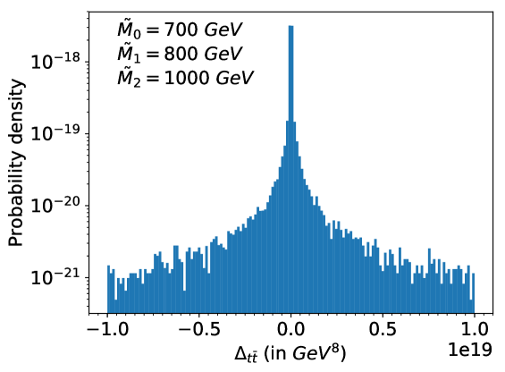
Figure 15: One-dimensional distribution of the singularity variable $\Delta_{t\bar{t}}(M_{2},M_{1},M_{0})$, computed with the true mass spectrum from Table 1. Note that the $y$-axis is plotted on a log scale.

One subtlety of the $\Delta_{t\bar{t}}$ computation is that there can be multiple (up to four) solutions (107) for the invisible momenta. In making Fig. 15, we made sure that each event contributes equally to the plot, by entering the result for each solution with a weight $1/N_{s}$, where $N_{s}$ is the total number of solutions found in that event.

Having derived the singularity variable for the event topology of Fig. 1(f), our next task would have been to illustrate the singularity surface in the relevant observable phase space, similarly to Fig. 4 (left panel) and Fig. 12. Unfortunately, the observable phase space in this case is nine-dimensional, and we shall not attempt to visualize it here. The third and final task, the demonstration of the focus point method, was already accomplished in Ref. Kim:2019prx .

8 Conclusions and Outlook

In this paper we outlined the general prescription for deriving a singularity variable for a given event topology with missing energy, i.e., where some of the final state particles are invisible in the detector. We then illustrated the procedure with several common event topologies shown in Fig. 1. We started with the case of a single two-body decay in Sec. 3 and re-derived the well known result that the distribution of the transverse mass $m_{T}$ has a Jacobian peak. In the subsequent sections, we demonstrated that similar Jacobian peak features are present in the distributions of the relevant kinematic variables for the remaining five event topologies. We also identified, parametrized and studied the shapes of the singularity surfaces in the appropriate visible phase spaces. In some special circumstances (see Secs. 3.2.1 and 4) the singularity variable can be computed directly in terms of the available kinematic information, without the need for any additional hypothesized inputs. However, more often than not, the singularity variable depends on the masses of the intermediate resonances and/or the masses of the invisible final state particles, and thus its computation requires a mass ansatz. If the event topology is applied to a SM process, the input masses will be known, but when applied to a BSM process, the mass ansatz is a priori unknown. However, this can be used to our benefit — it is precisely this dependence on the mass ansatz that makes the focus point method for mass measurements possible, as explicitly demonstrated in Sec. 3.3 and 6.3. The main advantage of the focus point method is that it maximally utilizes the singularity structures in phase space. As a consequence, the true masses are identified as a kinematic peak instead of a kinematic endpoint — endpoints are more difficult to observe experimentally, once we include the finite widths and detector resolution effects Chatrchyan:2013boa . It is also worthwhile to contrast the focus point method to the polynomial method Cheng:2007xv ; Cheng:2008mg ; Cheng:2009fw ; Webber:2009vm . While both methods use the same type of kinematic constraints, the latter requires a larger set of constraints in order to avoid the need for a mass ansatz.

The ideas presented in this paper may find immediate application in a large number of LHC analyses targeting the event topologies of Fig. 1.

• Standard Model measurements. Precision studies of SM processes typically require the identification of a specific event topology, e.g., Fig. 1(a) for $W$ production, Fig. 1(b) for top quark decay, Fig. 1(d) for $W$ pair-production, and Fig. 1(f) for dilepton $t\bar{t}$ production. The corresponding singularity variables are ideal for tagging such events, and may also be used as input features for event selectors based on machine learning.

• New physics searches. The Jacobian peaks in the distributions of the singularity variables can be used to discover new physics processes over the SM background Debnath:2018azt . Likewise, the peak structures in the heatmaps constructed in the focus point method can also be used for discovery of new physics, with the added advantage that background processes will not develop fake peaks in the signal regions.

In this paper we mostly focused on the case (9) when the number of unknowns $N_{q}$ matches the number of kinematic constraints $N_{C}$. However, the under-constrained case $N_{C}<N_{q}$ is also worth investigating, e.g., following the analysis of Ref. DeRujula:2012ns . All of these topics are being pursued in a future publication MS .

- (1) The ATLAS collaboration [ATLAS Collaboration], “Performance of Missing Transverse Momentum Reconstruction in ATLAS studied in Proton-Proton Collisions recorded in 2012 at 8 TeV,” ATLAS-CONF-2013-082.
- (2) CMS Collaboration [CMS Collaboration], “Performance of missing energy reconstruction in 13 TeV pp collision data using the CMS detector,” CMS-PAS-JME-16-004.
- (3) J. L. Feng, “Dark Matter Candidates from Particle Physics and Methods of Detection,” Ann. Rev. Astron. Astrophys. 48, 495 (2010) [arXiv:1003.0904 [astro-ph.CO]].
- (4) J. Hubisz, J. Lykken, M. Pierini and M. Spiropulu, “Missing energy look-alikes with 100 pb-1 at the LHC,” Phys. Rev. D 78, 075008 (2008) [arXiv:0805.2398 [hep-ph]].
- (5) B. W. Lee, C. Quigg and H. B. Thacker, “Weak Interactions at Very High-Energies: The Role of the Higgs Boson Mass,” Phys. Rev. D 16, 1519 (1977).
- (6) M. J. Duncan, G. L. Kane and W. W. Repko, “W W Physics at Future Colliders,” Nucl. Phys. B 272, 517 (1986).
- (7) S. Chatrchyan et al. [CMS Collaboration], “Measurement of Higgs boson production and properties in the WW decay channel with leptonic final states,” JHEP 1401, 096 (2014) [arXiv:1312.1129 [hep-ex]].
- (8) G. Aad et al. [ATLAS Collaboration], “Observation and measurement of Higgs boson decays to WW∗ with the ATLAS detector,” Phys. Rev. D 92, no. 1, 012006 (2015) [arXiv:1412.2641 [hep-ex]].
- (9) D. Alves et al. [LHC New Physics Working Group], “Simplified Models for LHC New Physics Searches,” J. Phys. G 39, 105005 (2012) [arXiv:1105.2838 [hep-ph]].
- (10) I. W. Kim, “Algebraic Singularity Method for Mass Measurement with Missing Energy,” Phys. Rev. Lett. 104, 081601 (2010) [arXiv:0910.1149 [hep-ph]].
- (11) A. Rujula and A. Galindo, “Measuring the W-Boson mass at a hadron collider: a study of phase-space singularity methods,” JHEP 1108, 023 (2011) [arXiv:1106.0396 [hep-ph]].
- (12) A. De Rujula and A. Galindo, “Singular ways to search for the Higgs boson,” JHEP 1206, 091 (2012) [arXiv:1202.2552 [hep-ph]].
- (13) D. Kim, K. T. Matchev and P. Shyamsundar, “Kinematic Focus Point Method for Particle Mass Measurements in Missing Energy Events,” arXiv:1906.02821 [hep-ph].
- (14) P. Sikivie, “Caustic rings of dark matter,” Phys. Lett. B 432, 139 (1998) [astro-ph/9705038].
- (15) T. K. Charles, D. M. Paganin and R. T. Dowd, “Caustic-based approach to understanding bunching dynamics and current spike formation in particle bunches,” Phys. Rev. Accel. Beams 19, no. 10, 104402 (2016).
- (16) D. Costanzo and D. R. Tovey, “Supersymmetric particle mass measurement with invariant mass correlations,” JHEP 0904, 084 (2009) [arXiv:0902.2331 [hep-ph]].
- (17) C. G. Lester, “Mass and Spin Measurement Techniques (for the Large Hadron Collider)”, lectures given at TASI 2011, Boulder, CO.
- (18) P. Agrawal, C. Kilic, C. White and J. H. Yu, “Improved Mass Measurement Using the Boundary of Many-Body Phase Space,” Phys. Rev. D 89, no. 1, 015021 (2014) [arXiv:1308.6560 [hep-ph]].
- (19) D. Kim, K. T. Matchev and M. Park, “Using sorted invariant mass variables to evade combinatorial ambiguities in cascade decays,” JHEP 1602, 129 (2016) [arXiv:1512.02222 [hep-ph]].
- (20) D. Debnath, J. S. Gainer, C. Kilic, D. Kim, K. T. Matchev and Y. P. Yang, “Identifying Phase Space Boundaries with Voronoi Tessellations,” Eur. Phys. J. C 76, no. 11, 645 (2016) [arXiv:1606.02721 [hep-ph]].
- (21) D. Debnath, J. S. Gainer, C. Kilic, D. Kim, K. T. Matchev and Y. P. Yang, “Detecting kinematic boundary surfaces in phase space: particle mass measurements in SUSY-like events,” JHEP 1706, 092 (2017) [arXiv:1611.04487 [hep-ph]].
- (22) B. Altunkaynak, C. Kilic and M. D. Klimek, “Multidimensional phase space methods for mass measurements and decay topology determination,” Eur. Phys. J. C 77, no. 2, 61 (2017) [arXiv:1611.09764 [hep-ph]].
- (23) D. Debnath, J. S. Gainer, D. Kim and K. T. Matchev, “Edge Detecting New Physics the Voronoi Way,” EPL 114, no. 4, 41001 (2016) [arXiv:1506.04141 [hep-ph]].
- (24) D. Debnath, J. S. Gainer, D. Kim and K. T. Matchev, “Discovering New Physics with Voronoi Tessellations,” arXiv:1511.02724 [hep-ph].
- (25) D. Debnath, J. S. Gainer, C. Kilic, D. Kim, K. T. Matchev and Y. P. Yang, “Enhancing the discovery prospects for SUSY-like decays with a forgotten kinematic variable,” JHEP 1905, 008 (2019) [arXiv:1809.04517 [hep-ph]].
- (26) Y. Bai, H. C. Cheng, J. Gallicchio and J. Gu, “Stop the Top Background of the Stop Search,” JHEP 1207, 110 (2012) [arXiv:1203.4813 [hep-ph]].
- (27) A. J. Barr and C. G. Lester, “A Review of the Mass Measurement Techniques proposed for the Large Hadron Collider,” J. Phys. G 37, 123001 (2010) [arXiv:1004.2732 [hep-ph]].
- (28) K. T. Matchev, F. Moortgat and L. Pape, “Dreaming Awake: Disentangling the Underlying Physics in Case of a SUSY-like Discovery at the LHC,” J. Phys. G 46, no. 11, 115002 (2019) [arXiv:1902.11267 [hep-ph]].
- (29) M. M. Nojiri, G. Polesello and D. R. Tovey, “Proposal for a new reconstruction technique for SUSY processes at the LHC,” hep-ph/0312317.
- (30) K. Kawagoe, M. M. Nojiri and G. Polesello, “A New SUSY mass reconstruction method at the CERN LHC,” Phys. Rev. D 71, 035008 (2005) [hep-ph/0410160].
- (31) H. C. Cheng and Z. Han, “Minimal Kinematic Constraints and m(T2),” JHEP 0812, 063 (2008) [arXiv:0810.5178 [hep-ph]].
- (32) B. Gripaios, K. Sakurai and B. Webber, “Polynomials, Riemann surfaces, and reconstructing missing-energy events,” JHEP 1109, 140 (2011) [arXiv:1103.3438 [hep-ph]].
- (33) G. Anagnostou, “Model Independent Search in 2-Dimensional Mass Space,” EPJ Web Conf. 71, 00006 (2014) [arXiv:1112.3379 [hep-ph]].
- (34) E. Byckling and K. Kajantie, “Particle Kinematics”, John Wiley & Sons, London, 1973.
- (35) V. D. Barger and R. J. N. Phillips, “Collider Physics,” REDWOOD CITY, USA: ADDISON-WESLEY (1987) 592 P. (FRONTIERS IN PHYSICS, 71)
- (36) A. J. Barr, T. J. Khoo, P. Konar, K. Kong, C. G. Lester, K. T. Matchev and M. Park, “Guide to transverse projections and mass-constraining variables,” Phys. Rev. D 84, 095031 (2011) [arXiv:1105.2977 [hep-ph]].
- (37) D. Kim and K. T. Matchev, “How to prove that a excess at the LHC is not due to dark matter,” Phys. Rev. D 98, no. 5, 055018 (2018) [arXiv:1712.07620 [hep-ph]].
- (38) J. Alwall, M. Herquet, F. Maltoni, O. Mattelaer and T. Stelzer, “MadGraph 5 : Going Beyond,” JHEP 1106, 128 (2011) [arXiv:1106.0522 [hep-ph]].
- (39) P. Baringer, K. Kong, M. McCaskey and D. Noonan, “Revisiting Combinatorial Ambiguities at Hadron Colliders with ,” JHEP 1110, 101 (2011) [arXiv:1109.1563 [hep-ph]].
- (40) K. Choi, D. Guadagnoli and C. B. Park, “Reducing combinatorial uncertainties: A new technique based on MT2 variables,” JHEP 1111, 117 (2011) [arXiv:1109.2201 [hep-ph]].
- (41) D. Debnath, D. Kim, J. H. Kim, K. Kong and K. T. Matchev, “Resolving Combinatorial Ambiguities in Dilepton Event Topologies with Constrained Variables,” Phys. Rev. D 96, no. 7, 076005 (2017) [arXiv:1706.04995 [hep-ph]].
- (42) K. T. Matchev and P. Shyamsundar, in preparation.
- (43) V. D. Barger, A. D. Martin and R. J. N. Phillips, “Perpendicular Mass From Decay,” Z. Phys. C 21, 99 (1983).
- (44) J. Smith, W. L. van Neerven and J. A. M. Vermaseren, “The Transverse Mass and Width of the Boson,” Phys. Rev. Lett. 50, 1738 (1983).
- (45) V. M. Abazov et al. [D0 Collaboration], “Measurement of the W Boson Mass with the D0 Detector,” Phys. Rev. Lett. 108, 151804 (2012) [arXiv:1203.0293 [hep-ex]].
- (46) T. A. Aaltonen et al. [CDF Collaboration], “Precise measurement of the W-boson mass with the Collider Detector at Fermilab,” Phys. Rev. D 89, no. 7, 072003 (2014) [arXiv:1311.0894 [hep-ex]].
- (47) M. Aaboud et al. [ATLAS Collaboration], “Measurement of the -boson mass in pp collisions at TeV with the ATLAS detector,” Eur. Phys. J. C 78, no. 2, 110 (2018) Erratum: [Eur. Phys. J. C 78, no. 11, 898 (2018)] [arXiv:1701.07240 [hep-ex]].
- (48) V. M. Abazov et al. [D0 Collaboration], “Search for bosons decaying to an electron and a neutrino with the D0 detector,” Phys. Rev. Lett. 100, 031804 (2008) [arXiv:0710.2966 [hep-ex]].
- (49) T. Aaltonen et al. [CDF Collaboration], “Search for a New Heavy Gauge Boson with Electron + missing ET Event Signature in collisions at TeV,” Phys. Rev. D 83, 031102 (2011) [arXiv:1012.5145 [hep-ex]].
- (50) A. M. Sirunyan et al. [CMS Collaboration], “Search for high-mass resonances in final states with a lepton and missing transverse momentum at TeV,” JHEP 1806, 128 (2018) [arXiv:1803.11133 [hep-ex]].
- (51) G. Aad et al. [ATLAS Collaboration], “Search for a heavy charged boson in events with a charged lepton and missing transverse momentum from collisions at TeV with the ATLAS detector,” arXiv:1906.05609 [hep-ex].
- (52) W. S. Cho, K. Choi, Y. G. Kim and C. B. Park, “Gluino Stransverse Mass,” Phys. Rev. Lett. 100, 171801 (2008) [arXiv:0709.0288 [hep-ph]].
- (53) B. Gripaios, “Transverse observables and mass determination at hadron colliders,” JHEP 0802, 053 (2008) [arXiv:0709.2740 [hep-ph]].
- (54) A. J. Barr, B. Gripaios and C. G. Lester, “Weighing Wimps with Kinks at Colliders: Invisible Particle Mass Measurements from Endpoints,” JHEP 0802, 014 (2008) [arXiv:0711.4008 [hep-ph]].
- (55) W. S. Cho, K. Choi, Y. G. Kim and C. B. Park, “Measuring superparticle masses at hadron collider using the transverse mass kink,” JHEP 0802, 035 (2008) [arXiv:0711.4526 [hep-ph]].
- (56) K. T. Matchev, F. Moortgat, L. Pape and M. Park, “Precision sparticle spectroscopy in the inclusive same-sign dilepton channel at LHC,” Phys. Rev. D 82, 077701 (2010) [arXiv:0909.4300 [hep-ph]].
- (57) G. G. Ross and M. Serna, “Mass determination of new states at hadron colliders,” Phys. Lett. B 665, 212 (2008) [arXiv:0712.0943 [hep-ph]].
- (58) A. J. Barr, G. G. Ross and M. Serna, “The Precision Determination of Invisible-Particle Masses at the LHC,” Phys. Rev. D 78, 056006 (2008) [arXiv:0806.3224 [hep-ph]].
- (59) P. Konar, K. Kong and K. T. Matchev, “ : A Global inclusive variable for determining the mass scale of new physics in events with missing energy at hadron colliders,” JHEP 0903, 085 (2009) [arXiv:0812.1042 [hep-ph]].
- (60) P. Konar, K. Kong, K. T. Matchev and M. Park, “RECO level and subsystem : Improved global inclusive variables for measuring the new physics mass scale in events at hadron colliders,” JHEP 1106, 041 (2011) [arXiv:1006.0653 [hep-ph]].
- (61) R. Mahbubani, K. T. Matchev and M. Park, “Re-interpreting the Oxbridge stransverse mass variable MT2 in general cases,” JHEP 1303, 134 (2013) [arXiv:1212.1720 [hep-ph]].
- (62) W. S. Cho, J. S. Gainer, D. Kim, K. T. Matchev, F. Moortgat, L. Pape and M. Park, “On-shell constrained variables with applications to mass measurements and topology disambiguation,” JHEP 1408, 070 (2014) [arXiv:1401.1449 [hep-ph]].
- (63) W. S. Cho, J. S. Gainer, D. Kim, K. T. Matchev, F. Moortgat, L. Pape and M. Park, “Improving the sensitivity of stop searches with on-shell constrained invariant mass variables,” JHEP 1505, 040 (2015) [arXiv:1411.0664 [hep-ph]].
- (64) D. Kim, H. S. Lee and M. Park, “Invisible dark gauge boson search in top decays using a kinematic method,” JHEP 1503, 134 (2015) [arXiv:1411.0668 [hep-ph]].
- (65) A. K. Swain and P. Konar, “Constrained and reconstructing with semi-invisible production at hadron colliders,” JHEP 1503, 142 (2015) [arXiv:1412.6624 [hep-ph]].
- (66) W. S. Cho, J. S. Gainer, D. Kim, S. H. Lim, K. T. Matchev, F. Moortgat, L. Pape and M. Park, “OPTIMASS: A Package for the Minimization of Kinematic Mass Functions with Constraints,” JHEP 1601, 026 (2016) [arXiv:1508.00589 [hep-ph]].
- (67) P. Konar and A. K. Swain, “Reconstructing semi-invisible events in resonant tau pair production from Higgs,” Phys. Lett. B 757, 211 (2016) [arXiv:1602.00552 [hep-ph]].
- (68) D. Goncalves, K. Kong and J. H. Kim, “Probing the top-Higgs Yukawa CP structure in dileptonic with M2-assisted reconstruction,” JHEP 1806, 079 (2018) [arXiv:1804.05874 [hep-ph]].
- (69) K. T. Matchev and M. Park, “A General method for determining the masses of semi-invisibly decaying particles at hadron colliders,” Phys. Rev. Lett. 107, 061801 (2011) [arXiv:0910.1584 [hep-ph]].
- (70) P. Konar, K. Kong, K. T. Matchev and M. Park, “Superpartner Mass Measurement Technique using 1D Orthogonal Decompositions of the Cambridge Transverse Mass Variable ,” Phys. Rev. Lett. 105, 051802 (2010) [arXiv:0910.3679 [hep-ph]].
- (71) T. Appelquist, H. C. Cheng and B. A. Dobrescu, “Bounds on universal extra dimensions,” Phys. Rev. D 64, 035002 (2001) [hep-ph/0012100].
- (72) T. G. Rizzo, “Probes of universal extra dimensions at colliders,” Phys. Rev. D 64, 095010 (2001) [hep-ph/0106336].
- (73) H. C. Cheng, K. T. Matchev and M. Schmaltz, “Bosonic supersymmetry? Getting fooled at the CERN LHC,” Phys. Rev. D 66, 056006 (2002) [hep-ph/0205314].
- (74) N. Arkani-Hamed, A. G. Cohen, E. Katz and A. E. Nelson, “The Littlest Higgs,” JHEP 0207, 034 (2002) [hep-ph/0206021].
- (75) H. C. Cheng and I. Low, “Little hierarchy, little Higgses, and a little symmetry,” JHEP 0408, 061 (2004) [hep-ph/0405243].
- (76) M. Schmaltz and D. Tucker-Smith, “Little Higgs review,” Ann. Rev. Nucl. Part. Sci. 55, 229 (2005) [hep-ph/0502182].
- (77) M. Perelstein, “Little Higgs models and their phenomenology,” Prog. Part. Nucl. Phys. 58, 247 (2007) [hep-ph/0512128].
- (78) C. Athanasiou, C. G. Lester, J. M. Smillie and B. R. Webber, “Distinguishing Spins in Decay Chains at the Large Hadron Collider,” JHEP 0608, 055 (2006) [hep-ph/0605286].
- (79) L. T. Wang and I. Yavin, “Spin measurements in cascade decays at the LHC,” JHEP 0704, 032 (2007) [hep-ph/0605296].
- (80) M. Burns, K. Kong, K. T. Matchev and M. Park, “A General Method for Model-Independent Measurements of Particle Spins, Couplings and Mixing Angles in Cascade Decays with Missing Energy at Hadron Colliders,” JHEP 0810, 081 (2008) [arXiv:0808.2472 [hep-ph]].
- (81) T. Han, I. W. Kim and J. Song, “Kinematic Cusps: Determining the Missing Particle Mass at Colliders,” Phys. Lett. B 693, 575 (2010) [arXiv:0906.5009 [hep-ph]].
- (82) M. Baumgart, T. Hartman, C. Kilic and L. T. Wang, “Discovery and measurement of sleptons, binos, and winos with a Z-prime,” JHEP 0711, 084 (2007) [hep-ph/0608172].
- (83) A. J. Barr, B. Gripaios and C. G. Lester, “Measuring the Higgs boson mass in dileptonic W-boson decays at hadron colliders,” JHEP 0907, 072 (2009) [arXiv:0902.4864 [hep-ph]].
- (84) K. Choi, S. Choi, J. S. Lee and C. B. Park, “Reconstructing the Higgs boson in dileptonic W decays at hadron collider,” Phys. Rev. D 80, 073010 (2009) [arXiv:0908.0079 [hep-ph]].
- (85) A. J. Barr, S. T. French, J. A. Frost and C. G. Lester, “Speedy Higgs boson discovery in decays to tau lepton pairs: ,” JHEP 1110, 080 (2011) [arXiv:1106.2322 [hep-ph]].
- (86) C. B. Park, “Reconstructing the heavy resonance at hadron colliders,” Phys. Rev. D 84, 096001 (2011) [arXiv:1106.6087 [hep-ph]].
- (87) A. J. Barr, B. Gripaios and C. G. Lester, “Re-weighing the evidence for a Higgs boson in dileptonic W-boson decays,” Phys. Rev. Lett. 108, 041803 (2012) Erratum: [Phys. Rev. Lett. 108, 109902 (2012)] [arXiv:1108.3468 [hep-ph]].
- (88) L. Edelhauser, K. T. Matchev and M. Park, “Spin effects in the antler event topology at hadron colliders,” JHEP 1211, 006 (2012) [arXiv:1205.2054 [hep-ph]].
- (89) T. Han, I. W. Kim and J. Song, “Kinematic Cusps With Two Missing Particles I: Antler Decay Topology,” Phys. Rev. D 87, no. 3, 035003 (2013) [arXiv:1206.5633 [hep-ph]].
- (90) P. Konar and A. K. Swain, “Mass reconstruction with under constraint in semi-invisible production at a hadron collider,” Phys. Rev. D 93, no. 1, 015021 (2016) [arXiv:1509.00298 [hep-ph]].
- (91) N. D. Christensen, T. Han, Z. Qian, J. Sayre, J. Song and Stefanus, “Determining the Dark Matter Particle Mass through Antler Topology Processes at Lepton Colliders,” Phys. Rev. D 90, 114029 (2014) [arXiv:1404.6258 [hep-ph]].
- (92) S. Y. Choi, N. D. Christensen, D. Salmon and X. Wang, “Spin and chirality effects in antler-topology processes at high energy colliders,” Eur. Phys. J. C 75, no. 10, 481 (2015) [arXiv:1503.02666 [hep-ph]].
- (93) J. L. Feng and D. E. Finnell, “Squark mass determination at the next generation of linear colliders,” Phys. Rev. D 49, 2369 (1994) [hep-ph/9310211].
- (94) L. A. Harland-Lang, C. H. Kom, K. Sakurai and W. J. Stirling, “Mass Shell Technique for Measuring Masses of a Pair of Semi-Invisibly Decaying Particles,” Phys. Rev. Lett. 108, 181805 (2012) [arXiv:1202.0047 [hep-ph]].
- (95) Q. F. Xiang, X. J. Bi, Q. S. Yan, P. F. Yin and Z. H. Yu, “Measuring Masses in Semi-Invisible Final States at Electron-Positron Colliders,” Phys. Rev. D 95, no. 7, 075037 (2017) [arXiv:1610.03372 [hep-ph]].
- (96) C. G. Lester and D. J. Summers, “Measuring masses of semiinvisibly decaying particles pair produced at hadron colliders,” Phys. Lett. B 463, 99 (1999) [hep-ph/9906349].
- (97) A. Barr, C. Lester and P. Stephens, “m(T2): The Truth behind the glamour,” J. Phys. G 29, 2343 (2003) [hep-ph/0304226].
- (98) M. Burns, K. Kong, K. T. Matchev and M. Park, “Using Subsystem MT2 for Complete Mass Determinations in Decay Chains with Missing Energy at Hadron Colliders,” JHEP 0903, 143 (2009) [arXiv:0810.5576 [hep-ph]].
- (99) A. J. Barr, B. Gripaios and C. G. Lester, “Transverse masses and kinematic constraints: from the boundary to the crease,” JHEP 0911, 096 (2009) [arXiv:0908.3779 [hep-ph]].
- (100) P. Konar, K. Kong, K. T. Matchev and M. Park, “Dark Matter Particle Spectroscopy at the LHC: Generalizing M(T2) to Asymmetric Event Topologies,” JHEP 1004, 086 (2010) [arXiv:0911.4126 [hep-ph]].
- (101) D. R. Tovey, “On measuring the masses of pair-produced semi-invisibly decaying particles at hadron colliders,” JHEP 0804, 034 (2008) [arXiv:0802.2879 [hep-ph]].
- (102) W. S. Cho, J. E. Kim and J. H. Kim, “Amplification of endpoint structure for new particle mass measurement at the LHC,” Phys. Rev. D 81, 095010 (2010) [arXiv:0912.2354 [hep-ph]].
- (103) W. S. Cho, W. Klemm and M. M. Nojiri, “Mass measurement in boosted decay systems at hadron colliders,” Phys. Rev. D 84, 035018 (2011) [arXiv:1008.0391 [hep-ph]].
- (104) W. S. Cho, K. Choi, Y. G. Kim and C. B. Park, “M(T2)-assisted on-shell reconstruction of missing momenta and its application to spin measurement at the LHC,” Phys. Rev. D 79, 031701 (2009) [arXiv:0810.4853 [hep-ph]].
- (105) D. Guadagnoli and C. B. Park, “-reconstructed invisible momenta as spin analizers, and an application to top polarization,” JHEP 1401, 030 (2014) [arXiv:1308.2226 [hep-ph]].
- (106) L. Sonnenschein, “Algebraic approach to solve dilepton equations,” Phys. Rev. D 72, 095020 (2005) [hep-ph/0510100].
- (107) L. Sonnenschein, “Analytical solution of ttbar dilepton equations,” Phys. Rev. D 73, 054015 (2006) Erratum: [Phys. Rev. D 78, 079902 (2008)] [hep-ph/0603011].
- (108) B. A. Betchart, R. Demina and A. Harel, “Analytic solutions for neutrino momenta in decay of top quarks,” Nucl. Instrum. Meth. A 736, 169 (2014) [arXiv:1305.1878 [hep-ph]].
- (109) S. Chatrchyan et al. [CMS Collaboration], “Measurement of masses in the system by kinematic endpoints in pp collisions at = 7 TeV,” Eur. Phys. J. C 73, 2494 (2013) [arXiv:1304.5783 [hep-ex]].
- (110) H. C. Cheng, J. F. Gunion, Z. Han, G. Marandella and B. McElrath, “Mass determination in SUSY-like events with missing energy,” JHEP 0712, 076 (2007) [arXiv:0707.0030 [hep-ph]].
- (111) H. C. Cheng, D. Engelhardt, J. F. Gunion, Z. Han and B. McElrath, “Accurate Mass Determinations in Decay Chains with Missing Energy,” Phys. Rev. Lett. 100, 252001 (2008) [arXiv:0802.4290 [hep-ph]].
- (112) H. C. Cheng, J. F. Gunion, Z. Han and B. McElrath, “Accurate Mass Determinations in Decay Chains with Missing Energy. II,” Phys. Rev. D 80, 035020 (2009) [arXiv:0905.1344 [hep-ph]].
- (113) B. Webber, “Mass determination in sequential particle decay chains,” JHEP 0909, 124 (2009) [arXiv:0907.5307 [hep-ph]].