Searching for the odderon in $pp\to ppK^{+}K^{-}$ and $pp\to pp\mu^{+}\mu^{-}$ reactions in the $\phi(1020)$ resonance region at the LHC

Abstract

We explore the possibility of observing odderon exchange in the $pp\to ppK^{+}K^{-}$ and $pp\to pp\mu^{+}\mu^{-}$ reactions at the LHC. We consider the central exclusive production (CEP) of the $\phi(1020)$ resonance decaying into $K^{+}K^{-}$ and $\mu^{+}\mu^{-}$. We compare the purely diffractive contribution (odderon-pomeron fusion) to the photoproduction contribution (photon-pomeron fusion). The theoretical results are calculated within the tensor-pomeron and vector-odderon model for soft reactions. We include absorptive corrections at the amplitude level. In order to fix the coupling constants for the photon-pomeron fusion contribution we discuss the reactions $\gamma p\to\omega p$ and $\gamma p\to\phi p$ including $\phi$-$\omega$ mixing. We compare our results for these reactions with the available data, especially those from HERA. Our coupling constants for the pomeron-odderon-$\phi$ vertex are taken from an analysis of the WA102 data for the $pp\to pp\phi$ reaction. We show that the odderon-exchange contribution significantly improves the description of the $pp$ azimuthal correlations and the ${\rm dP_{t}}$ “glueball-filter variable” dependence of $\phi$ CEP measured by WA102. To describe the low-energy data more accurately we consider also subleading processes with reggeized vector-meson exchanges. However, they do not play a significant role at the LHC. We present predictions for two possible types of measurements: at midrapidity and with forward measurement of protons (relevant for ATLAS-ALFA or CMS-TOTEM), and at forward rapidities and without measurement of protons (relevant for LHCb). We discuss the influence of experimental cuts on the integrated cross sections and on various differential distributions. With the corresponding LHC data one should be able to get a decisive answer concerning the presence of an odderon-pomeron fusion contribution in single $\phi$ CEP.

I Introduction

So far there is no unambiguous experimental evidence for the odderon ($\mathbb{O}$), the charge conjugation $C=-1$ counterpart of the $C=+1$ pomeron ($\mathbb{P}$), introduced on theoretical grounds in Lukaszuk:1973nt ; Joynson:1975az and predicted in QCD as the exchange of a colourless $C$-odd three-gluon compound state Kwiecinski:1980wb ; Bartels:1980pe ; Jaroszewicz:1981jz ; Janik:1998xj ; Bartels:1999yt . A hint of the odderon was seen in ISR results Breakstone:1985pe as a small difference between the differential cross sections of elastic proton-proton ($pp$) and proton-antiproton ($p\bar{p}$) scattering in the diffractive dip region at $\sqrt{s}=53$ GeV. The interpretation of this difference is, however, complicated due to non-negligible contributions from secondary reggeons. Recently the TOTEM Collaboration has published data from high-energy elastic proton-proton scattering experiments at the LHC. In Antchev:2017yns results were given for the $\rho$ parameter, the ratio of real to imaginary part of the forward scattering amplitude. This is a measurement at $t=0$. In Antchev:2018rec the differential cross section $d\sigma/dt$ was measured for 0.36 GeV${}^{2}<|t|<0.74$ GeV². The interpretation of these results is controversial at the moment. Some authors claim for instance that the $\rho$ measurements show that there must be an odderon effect at $t=0$ Martynov:2017zjz ; Martynov:2018nyb . But other authors find that no odderon contribution is needed at $t=0$ Khoze:2017swe ; Khoze:2018bus ; Khoze:2018kna ; Broilo:2018qqs ; Donnachie:2019ciz . For a general analysis of $pp$ and $p\bar{p}$ elastic scattering see, e.g., Csorgo:2018uyp ; Bence:2018ain .

As was discussed in Schafer:1991na exclusive diffractive $J/\psi$ and $\phi$ production from the pomeron-odderon fusion in high-energy $pp$ and $p\bar{p}$ collisions is a direct probe for a possible odderon exchange. The photoproduction mechanism (i.e., pomeron-photon fusion) constitutes a background for pomeron-odderon exchanges in these reactions. Other sources of background involve secondary reggeon exchanges, for instance pomeron-($\phi_{\mathbb{R}}$-reggeon) exchanges. Exclusive production of heavy vector mesons, $J/\psi$ and $\Upsilon$, from the pomeron-odderon and the pomeron-photon fusion in the pQCD $k_{t}$-factorization approach was discussed in Bzdak:2007cz . The exclusive $pp\to pp\phi$ reaction via the (pQCD-pomeron)-photon fusion in the high-energy corner was studied in Cisek:2010jk ; see also Cisek:2014ala for the exclusive photoproduction of charmonia $J/\psi$ and $\psi^{\prime}$ and Cisek:2011vt for the exclusive $\omega$ production.

A possible probe of the odderon is photoproduction of $C=+1$ mesons Schafer:1992pq ; Barakhovsky:1991ra . At sufficiently high energies only odderon and photon exchange contribute to these reactions. Photoproduction of the pseudoscalars $\pi^{0}$, $\eta$, $\eta^{\prime}$, $\eta_{c}$, and of the tensor $f_{2}(1270)$ in $ep$ scattering at high energies was discussed in Kilian:1997ew ; Berger:1999ca ; Berger:2000wt ; Donnachie:2005bu ; Ewerz:2006gd . For exclusive $\eta_{c}$ photoproduction within the high-energy framework of eikonal dipole scattering see Dumitru:2019qec . In Motyka:1998kb ; Braunewell:2004pf a probe of the perturbative odderon in the quasidiffractive process $\gamma^{*}\gamma^{*}\to\eta_{c}\eta_{c}$ was studied.

Another interesting possibility is to study the charge asymmetry caused by the interference between pomeron and odderon exchange. This was discussed in diffractive $c\bar{c}$ pair photoproduction Brodsky:1999mz , in diffractive $\pi^{+}\pi^{-}$ pair photoproduction Hagler:2002nh ; Hagler:2002nf ; Ginzburg:2002zd ; Bolz:2014mya , and in the production of two pion pairs in photon-photon collisions Pire:2008xe . However, so far in no one of the exclusive reactions a clear identification of the odderon was found experimentally. For a more detailed review of the phenomenological and theoretical status of the odderon we refer the reader to Ewerz:2003xi ; Ewerz:2005rg . In this context we would also like to mention the EMMI workshop on “Central exclusive production at the LHC” which was held in Heidelberg in February 2019. There, questions of odderon searches were extensively discussed. Corresponding remarks and the link to the talks presented at this workshop can be found in Ewerz:2019arb .

Recently, the possibility of probing the odderon in ultraperipheral proton-ion collisions was considered Goncalves:2018pbr ; Harland-Lang:2018ytk . In Goncalves:2015hra the measurement of the exclusive $\eta_{c}$ production in nuclear collisions was discussed. The situation of the odderon in this context is also not obvious and requires further studies.

In Ewerz:2013kda the tensor-pomeron and vector-odderon concept was introduced for soft reactions. In this approach, the $C=+1$ pomeron and the reggeons $\mathbb{R}_{+}=f_{2\mathbb{R}},a_{2\mathbb{R}}$ are treated as effective rank-2 symmetric tensor exchanges while the $C=-1$ odderon and the reggeons $\mathbb{R}_{-}=\omega_{\mathbb{R}},\rho_{\mathbb{R}}$ are treated as effective vector exchanges. For these effective exchanges a number of propagators and vertices, respecting the standard rules of quantum field theory, were derived from comparisons with experiments. This allows for an easy construction of amplitudes for specific processes. In Ewerz:2016onn the helicity structure of small-$|t|$ proton-proton elastic scattering was considered in three models for the pomeron: tensor, vector, and scalar. Only the tensor ansatz for the pomeron was found to be compatible with the high-energy experiment on polarised $pp$ elastic scattering Adamczyk:2012kn . In Britzger:2019lvc the authors, using combinations of two tensor-type pomerons (a soft one and a hard one) and the $\mathbb{R}_{+}$-reggeon exchange, successfully described low-$x$ deep-inelastic lepton-nucleon scattering and photoproduction.

Applications of the tensor-pomeron and vector-odderon ansatz were given for photoproduction of pion pairs in Bolz:2014mya and for a number of central-exclusive-production (CEP) reactions in proton-proton collisions in Lebiedowicz:2013ika ; Lebiedowicz:2014bea ; Lebiedowicz:2016ioh ; Lebiedowicz:2016zka ; Lebiedowicz:2016ryp ; Lebiedowicz:2018sdt ; Lebiedowicz:2018eui ; Lebiedowicz:2019jru ; Lebiedowicz:2019por . Also contributions from the subleading exchanges, $\mathbb{R}_{+}$ and $\mathbb{R}_{-}$, were discussed in these works. As an example, for the $pp\to ppp\bar{p}$ reaction Lebiedowicz:2018sdt the contributions involving the odderon are expected to be small since its coupling to the proton is very small. We have predicted asymmetries in the (pseudo)rapidity distributions of the centrally produced antiproton and proton. The asymmetry is caused by interference effects of the dominant ($\mathbb{P},\mathbb{P}$) with the subdominant ($\mathbb{O}+\mathbb{R}_{-}$, $\mathbb{P}+\mathbb{R}_{+}$) and ($\mathbb{P}+\mathbb{R}_{+}$, $\mathbb{O}+\mathbb{R}_{-}$) exchanges. We find for the odderon only very small effects, roughly a factor 10 smaller than the effects due to reggeons.

In this paper we consider the possibility of observing odderon exchange in the $pp\to pp\phi$, $pp\to pp(\phi\to K^{+}K^{-})$, and $pp\to pp(\phi\to\mu^{+}\mu^{-})$ reactions in the light of our recent analysis of the $pp\to pp\phi\phi$ reaction Lebiedowicz:2019jru . In the diffractive production of $\phi$ meson pairs it is possible to have pomeron-pomeron fusion with intermediate $\hat{t}/\hat{u}$-channel odderon exchange. Thus, the $pp\to pp\phi\phi$ reaction is a good candidate for the odderon-exchange searches, as it does not involve the coupling of the odderon to the proton. By confronting our model results, including the odderon, the reggeized $\phi$ exchange, and the $f_{2}(2340)$ resonance exchange contributions, with the WA102 data from Barberis:1998bq we derived an upper limit for the $\mathbb{P}\mathbb{O}\phi$ coupling. Taking into account typical kinematic cuts for LHC experiments in the $pp\to pp\phi\phi\to ppK^{+}K^{-}K^{+}K^{-}$ reaction we have found that the odderon exchange contribution should be distinguishable from other contributions for large rapidity distance between the outgoing $\phi$ mesons and in the region of large four-kaon invariant masses. At least, it should be possible to derive an upper limit on the odderon contribution in this reaction.

Here we will try to understand the $pp\to pp\phi$ reaction at relatively low center-of-mass energy $\sqrt{s}=29.1$ GeV by comparing our model results with the WA102 experimental data from Kirk:2000ws . We shall calculate the photoproduction mechanism. For this purpose we have to consider also low-energy photon-proton collisions in the $\gamma p\to\phi p$ reaction where the corresponding mechanism is not well established yet; see, e.g., Refs. Laget:2000gj ; Oh:2001bq ; Titov:1999eu ; Titov:2003bk ; Ozaki:2009mj ; Kiswandhi:2010ub ; Kiswandhi:2011cq ; Ryu:2012tw ; Kong:2016scm ; Kim:2019kef . Of course, the amplitude for $\gamma p\to\phi p$ cannot be realised by the $C=-1$ odderon exchange. In addition to the $\gamma$-$\mathbb{P}$-fusion processes we shall estimate also subleading contributions, e.g. the $\gamma$-pseudoscalar-meson fusion, the $\phi$-$\mathbb{P}$ fusion, the $\omega$-$\mathbb{P}$ fusion, the $\omega$-$f_{2\mathbb{R}}$ fusion, and the $\rho$-$\pi^{0}$ fusion, to determine their role in the $pp\to pp\phi$ reaction. Our aim is to see how much room is left for the $\mathbb{O}$-$\mathbb{P}$ fusion which is the main object of our studies.

Our paper is organized as follows. In Sec. II we consider the $pp\to pp(\phi\to K^{+}K^{-})$ reaction. Section III deals with $\mu^{+}\mu^{-}$ production. For both reactions we give analytic expressions for the resonant amplitudes. Section IV contains the comparison of our results for the $pp\to pp\phi$ reaction with the WA102 data. We discuss the role of different contributions such as $\gamma$-$\mathbb{P}$, $\mathbb{O}$-$\mathbb{P}$, $\phi$-$\mathbb{P}$, $\omega$-$\mathbb{P}$, and $\omega$-$f_{2\mathbb{R}}$ fusion processes. Then we turn to high energies and show numerical results for total and differential cross sections calculated with typical experimental cuts for the LHC experiments. We discuss our predictions for the $K^{+}K^{-}$ channel for $\sqrt{s}=13$ TeV. In addition, we present our predictions for the $\mu^{+}\mu^{-}$ production also at $\sqrt{s}=13$ TeV which is currently under analysis by the LHCb Collaboration. We briefly discuss and/or provide references to relevant works for the continuum contributions. Section V presents our conclusions and further prospects. In Appendices A and B we discuss useful relations and properties concerning the photoproduction of $\omega$ and $\phi$ mesons. In Appendix C we discuss the subleading processes contributing to $pp\to pp(\phi\to K^{+}K^{-})$. We have collected there some useful formulas concerning details of the calculations. In Appendix D we give the definition of the Collins-Soper (CS) frame used in our paper.

In our paper we denote by $e>0$ the proton charge. We use the $\gamma$-matrix conventions of Bjorken and Drell Bjorken_Drell_1965 . The totally antisymmetric Levi-Civita symbol $\varepsilon_{\mu\nu\kappa\lambda}$ is used with the normalisation $\varepsilon_{0123}=1$.

II The $pp\to pp\phi\to ppK^{+}K^{-}$ reaction

Here we discuss the reaction

$$p(p_{a},\lambda_{a})+p(p_{b},\lambda_{b})\to p(p_{1},\lambda_{1})+K^{+}(p_{3})+K^{-}(p_{4})+p(p_{2},\lambda_{2})\,,$$ (1)

where $p_{a,b}$, $p_{1,2}$ and $\lambda_{a,b},\lambda_{1,2}=\pm\frac{1}{2}$ denote the four-momenta and helicities of the protons and $p_{3,4}$ denote the four-momenta of the $K$ mesons, respectively.

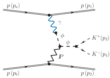
(a) (b)

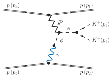
Figure 1: The Born-level diagrams for central exclusive $\phi$-meson photoproduction in proton-proton collisions with the subsequent decay $\phi\to K^{+}K^{-}$: (a) photon-pomeron fusion; (b) pomeron-photon fusion.

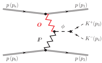
(a) (b)

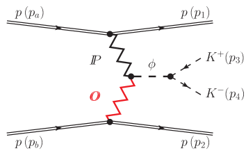
Figure 2: The Born-level diagrams for diffractive production of a $\phi$ meson decaying to $K^{+}K^{-}$ in proton-proton collisions with odderon exchange: (a) odderon-pomeron fusion; (b) pomeron-odderon fusion.

The full amplitude of the reaction (1) is a sum of the continuum amplitude and the amplitudes through the $s$-channel resonances as was discussed in detail in Lebiedowicz:2018eui . Here we focus on the limited dikaon invariant mass region, i.e., the $\phi\equiv\phi(1020)$ resonance region,

$$1.01\;\mathrm{GeV}<M_{K^{+}K^{-}}<1.03\;\mathrm{GeV}\,.$$ (2)

That is, we consider the reaction

$$p(p_{a},\lambda_{a})+p(p_{b},\lambda_{b})\to p(p_{1},\lambda_{1})+\left[\phi(p_{34})\to K^{+}(p_{3})+K^{-}(p_{4})\right]+p(p_{2},\lambda_{2})\,.$$ (3)

The kinematic variables are

$$p_{34}=p_{3}+p_{4}\,,\quad q_{1}=p_{a}-p_{1}\,,\quad q_{2}=p_{b}-p_{2}\,,$$

$$s=(p_{a}+p_{b})^{2}=(p_{1}+p_{2}+p_{34})^{2}\,,$$

$$t_{1}=q_{1}^{2}\,,\quad t_{2}=q_{2}^{2}\,,$$

$$s_{1}=(p_{1}+p_{34})^{2}\,,\quad s_{2}=(p_{2}+p_{34})^{2}\,.$$ (4)

For high energies and central $\phi$ production we expect the process (3) to be dominated by diffractive scattering. The corresponding diagrams are shown in Figs. 1 and 2. That is, we consider the fusion processes $\gamma\mathbb{P}\to\phi$ and $\mathbb{O}\mathbb{P}\to\phi$. For the first process all couplings are, in essence, known. For the odderon-exchange process we shall use the ansätze from Ewerz:2013kda and we shall try to get information on the odderon parameters and couplings from the reaction (3). The amplitude for (3) gets the following contributions from these diagrams

$${}^{(1)}{\cal M}_{pp\to ppK^{+}K^{-}}^{(\phi\to K^{+}K^{-})}={\cal M}^{(\gamma\mathbb{P})}_{pp\to ppK^{+}K^{-}}+{\cal M}^{(\mathbb{P}\gamma)}_{pp\to ppK^{+}K^{-}}\,,$$ (5)

$${}^{(2)}{\cal M}_{pp\to ppK^{+}K^{-}}^{(\phi\to K^{+}K^{-})}={\cal M}^{(\mathbb{O}\mathbb{P})}_{pp\to ppK^{+}K^{-}}+{\cal M}^{(\mathbb{P}\mathbb{O})}_{pp\to ppK^{+}K^{-}}\,.$$ (6)

At the relatively low center-of-mass energy of the WA102 experiment, $\sqrt{s}=29.1$ GeV, we have to include also subleading contributions with meson exchanges discussed in Appendix C.

To give the full physical amplitude, for instance, for the $pp\to ppK^{+}K^{-}$ process (1) we should include absorptive corrections to the Born amplitudes. For the details how to include the $pp$-rescattering corrections in the eikonal approximation for the four-body reaction see, e.g., Sec. 3.3 of Lebiedowicz:2014bea and Lebiedowicz:2015eka .

Below, in Table 2 of Sec. IV.2, we give numerical values for the gap survival factors (“soft survival probability” factors) denoted as $\langle S^{2}\rangle$, the ratios of full (including absorption) and Born cross sections.

The measurement of forward protons would be useful to better understand absorption effects. The GenEx Monte Carlo generator Kycia:2014hea ; Kycia:2017ota could be used in this context. We refer the reader to Kycia:2017iij where a first calculation of four-pion continuum production in the $pp\to pp\pi^{+}\pi^{-}\pi^{+}\pi^{-}$ reaction with the help of the GenEx code was performed.

II.1 $\gamma$-$\mathbb{P}$ fusion

The Born-level amplitude for the $\gamma$-$\mathbb{P}$ exchange, see diagram (a) in Fig. 1, reads

$${\cal M}^{(\gamma\mathbb{P})}_{pp\to ppK^{+}K^{-}}=(-i)\bar{u}(p_{1},\lambda_{1})i\Gamma^{(\gamma pp)}_{\mu}(p_{1},p_{a})u(p_{a},\lambda_{a})$$

$$\qquad\times i\Delta^{(\gamma)\,\mu\sigma}(q_{1})\,i\Gamma^{(\gamma\to\phi)}_{\sigma\nu}(q_{1})\,i\Delta^{(\phi)\,\nu\rho_{1}}(q_{1})\,i\Gamma^{(\mathbb{P}\phi\phi)}_{\rho_{2}\rho_{1}\alpha\beta}(p_{34},q_{1})\,i\Delta^{(\phi)\,\rho_{2}\kappa}(p_{34})\,i\Gamma^{(\phi KK)}_{\kappa}(p_{3},p_{4})$$

$$\qquad\times i\Delta^{(\mathbb{P})\,\alpha\beta,\delta\eta}(s_{2},t_{2})\,\bar{u}(p_{2},\lambda_{2})i\Gamma^{(\mathbb{P}pp)}_{\delta\eta}(p_{2},p_{b})u(p_{b},\lambda_{b})\,.$$ (7)

The $\gamma pp$ vertex and the photon propagator are given in Ewerz:2013kda by formulas (3.26) and (3.1), respectively. The $\gamma\to\phi$ transition is made here through the vector-meson-dominance (VMD) model; see (3.23)–(3.25) of Ewerz:2013kda . $\Delta^{(\mathbb{P})}$ and $\Gamma^{(\mathbb{P}pp)}$ denote the effective propagator and proton vertex function, respectively, for the tensorial pomeron. The corresponding expressions, as given in Sec. 3 of Ewerz:2013kda , are as follows

$$i\Delta^{(\mathbb{P})}_{\mu\nu,\kappa\lambda}(s,t)=\frac{1}{4s}\left(g_{\mu\kappa}g_{\nu\lambda}+g_{\mu\lambda}g_{\nu\kappa}-\frac{1}{2}g_{\mu\nu}g_{\kappa\lambda}\right)(-is\alpha^{\prime}_{\mathbb{P}})^{\alpha_{\mathbb{P}}(t)-1}\,,$$ (8)

$$i\Gamma_{\mu\nu}^{(\mathbb{P}pp)}(p^{\prime},p)=-i3\beta_{\mathbb{P}NN}F_{1}(t)\left\{\frac{1}{2}\left[\gamma_{\mu}(p^{\prime}+p)_{\nu}+\gamma_{\nu}(p^{\prime}+p)_{\mu}\right]-\frac{1}{4}g_{\mu\nu}(\not\!p^{\prime}+\not\!p)\right\},\qquad$$ (9)

where $t=(p^{\prime}-p)^{2}$ and $\beta_{\mathbb{P}NN}=1.87$ GeV^-1. For simplicity we use for the pomeron-nucleon coupling the electromagnetic Dirac form factor $F_{1}(t)$ of the proton. The pomeron trajectory $\alpha_{\mathbb{P}}(t)$ is assumed to be of standard linear form, see e.g. Donnachie:1992ny ; Donnachie:2002en ,

$$\alpha_{\mathbb{P}}(t)=\alpha_{\mathbb{P}}(0)+\alpha^{\prime}_{\mathbb{P}}\,t\,,$$ (10)

$$\alpha_{\mathbb{P}}(0)=1.0808\,,\;\;\alpha^{\prime}_{\mathbb{P}}=0.25\;\mathrm{GeV}^{-2}\,.$$ (11)

Our ansatz for the $\mathbb{P}\phi\phi$ vertex follows the one for the $\mathbb{P}\rho\rho$ in (3.47) of Ewerz:2013kda with the replacements $a_{\mathbb{P}\rho\rho}\to a_{\mathbb{P}\phi\phi}$ and $b_{\mathbb{P}\rho\rho}\to b_{\mathbb{P}\phi\phi}$. This was already used in Sec. IV B of Lebiedowicz:2018eui . The $\mathbb{P}\phi\phi$ vertex function is taken with the same Lorentz structure as for the $f_{2}\gamma\gamma$ coupling defined in (3.39) of Ewerz:2013kda . With $k^{\prime},\mu$ and $k,\nu$ the momentum and vector index of the outgoing and incoming $\phi$, respectively, and $\kappa\lambda$ the pomeron indices the $\mathbb{P}\phi\phi$ vertex reads

$$i\Gamma^{(\mathbb{P}\phi\phi)}_{\mu\nu\kappa\lambda}(k^{\prime},k) = iF_{M}((k^{\prime}-k)^{2})\,\tilde{F}^{(\phi)}(k^{\prime 2})\,\tilde{F}^{(\phi)}(k^{2})$$ (12)

$$\times\left[2a_{\mathbb{P}\phi\phi}\,\Gamma^{(0)}_{\mu\nu\kappa\lambda}(k^{\prime},-k)\,-b_{\mathbb{P}\phi\phi}\,\Gamma^{(2)}_{\mu\nu\kappa\lambda}(k^{\prime},-k)\right]\,,$$

with form factors $F_{M}$ and $\tilde{F}^{(\phi)}$ and two rank-four tensor functions,

$$\Gamma_{\mu\nu\kappa\lambda}^{(0)}(k_{1},k_{2})=\Big{[}(k_{1}\cdot k_{2})g_{\mu\nu}-k_{2\mu}k_{1\nu}\Big{]}\Big{[}k_{1\kappa}k_{2\lambda}+k_{2\kappa}k_{1\lambda}-\frac{1}{2}(k_{1}\cdot k_{2})g_{\kappa\lambda}\Big{]}\,,$$ (13)

$$\Gamma_{\mu\nu\kappa\lambda}^{(2)}(k_{1},k_{2})=\,(k_{1}\cdot k_{2})(g_{\mu\kappa}g_{\nu\lambda}+g_{\mu\lambda}g_{\nu\kappa})+g_{\mu\nu}(k_{1\kappa}k_{2\lambda}+k_{2\kappa}k_{1\lambda})$$

$$\qquad\qquad\qquad\quad-k_{1\nu}k_{2\lambda}g_{\mu\kappa}-k_{1\nu}k_{2\kappa}g_{\mu\lambda}-k_{2\mu}k_{1\lambda}g_{\nu\kappa}-k_{2\mu}k_{1\kappa}g_{\nu\lambda}$$

$$\qquad\qquad\qquad\quad-[(k_{1}\cdot k_{2})g_{\mu\nu}-k_{2\mu}k_{1\nu}]\,g_{\kappa\lambda}\,.$$ (14)

For details see Eqs. (3.18)–(3.22) of Ewerz:2013kda . In (12) the coupling parameters $a_{\mathbb{P}\phi\phi}$ and $b_{\mathbb{P}\phi\phi}$ have dimensions GeV^-3 and GeV^-1, respectively. In Lebiedowicz:2018eui we have fixed the coupling parameters of the tensor pomeron to the $\phi$ meson based on the HERA experimental data for the $\gamma p\to\phi p$ reaction Derrick:1996af ; Breitweg:1999jy . However, the $\omega$-$\phi$ mixing effect was not taken into account there. In the calculation here we include the $\omega$-$\phi$ mixing and we take the coupling parameters found in Appendix B.

The full form of the vector-meson propagator is given by (3.2) of Ewerz:2013kda . Using the properties of the tensorial functions (13) and (II.1), see (3.18)–(3.22) of Ewerz:2013kda , we can make for the $\phi$-meson propagator the following replacement

$$\Delta^{(\phi)}_{\mu\nu}(k)\to-g_{\mu\nu}\,\Delta^{(\phi)}_{T}(k^{2})\,,$$ (15)

where we take the simple Breit-Wigner expression, as discussed in Lebiedowicz:2018eui ,

$$\Delta_{T}^{(\phi)}(s)=\frac{1}{s-m_{\phi}^{2}+i\sqrt{s}\Gamma_{\phi}(s)}\,,$$ (16)

$$\Gamma_{\phi}(s)=\Gamma_{\phi}\left(\frac{s-4m_{K}^{2}}{m_{\phi}^{2}-4m_{K}^{2}}\right)^{3/2}\frac{m_{\phi}^{2}}{s}\,\theta(s-4m_{K}^{2})\,.$$ (17)

For the $\phi KK$ vertex we have from (4.24)–(4.26) of Lebiedowicz:2018eui

$$i\Gamma^{(\phi KK)}_{\kappa}(p_{3},p_{4})=-\frac{i}{2}\,g_{\phi K^{+}K^{-}}\,\left(p_{3}-p_{4}\right)_{\kappa}\,F^{(\phi KK)}(p_{34}^{2})$$ (18)

with $g_{\phi K^{+}K^{-}}=8.92$ and $F^{(\phi KK)}$ a form factor.

In the hadronic vertices we take into account corresponding form factors. We insert in the $\mathbb{P}\phi\phi$ vertex (12) the form factor $F_{M}(k^{2})$ to take into account the extended nature of $\phi$ mesons and $\tilde{F}^{(\phi)}(k^{2})$ since we are dealing with two off-shell $\phi$ mesons; see (4.27) of Lebiedowicz:2018eui and (B.85) of Bolz:2014mya . Convenient forms are

$$F_{M}(k^{2})=\frac{1}{1-k^{2}/\Lambda_{0,\,\mathbb{P}\phi\phi}^{2}}\,,$$ (19)

$$\tilde{F}^{(\phi)}(k^{2})=\left[1+\dfrac{k^{2}(k^{2}-m_{\phi}^{2})}{\tilde{\Lambda}_{\phi}^{4}}\right]^{-\tilde{n}_{\phi}},\quad\tilde{\Lambda}_{\phi}=2\;{\rm GeV}\,,\quad\tilde{n}_{\phi}=0.5\,.$$ (20)

We have $\tilde{F}^{(\phi)}(0)=\tilde{F}^{(\phi)}(m_{\phi})=1$. In (19) we take $\Lambda_{0,\,\mathbb{P}\phi\phi}^{2}=1.0$ GeV² (set A) or $\Lambda_{0,\,\mathbb{P}\phi\phi}^{2}=4.0$ GeV² (set B); see Fig. 31 of Appendix B. In practical calculations we include also in the $\phi KK$ vertex the form factor [see (4.28) of Lebiedowicz:2018eui ]

$$F^{(\phi KK)}(k^{2})=\exp{\left(\frac{-(k^{2}-m_{\phi}^{2})^{2}}{\Lambda_{\phi}^{4}}\right)}\,,\quad\Lambda_{\phi}=1\;{\rm GeV}\,.$$ (21)

Inserting all this in (7) we can write the amplitude for the $\gamma\mathbb{P}$ fusion as follows

$${\cal M}^{(\gamma\mathbb{P})}_{pp\to ppK^{+}K^{-}}=-i\,e^{2}\,\bar{u}(p_{1},\lambda_{1})\left[\gamma^{\alpha}F_{1}(t_{1})+\frac{i}{2m_{p}}\sigma^{\alpha\alpha^{\prime}}(p_{1}-p_{a})_{\alpha^{\prime}}F_{2}(t_{1})\right]u(p_{a},\lambda_{a})$$

$$\qquad\times\frac{1}{t_{1}}\,\frac{(-m_{\phi}^{2})}{t_{1}-m_{\phi}^{2}}\,\frac{1}{\gamma_{\phi}}\Delta_{T}^{(\phi)}(p_{34}^{2})\,\frac{g_{\phi K^{+}K^{-}}}{2}\,(p_{3}-p_{4})^{\beta}\,F^{(\phi KK)}(p_{34}^{2})$$

$$\qquad\times\left[2a_{\mathbb{P}\phi\phi}\,\Gamma^{(0)}_{\beta\alpha\kappa\lambda}(p_{34},-q_{1})-b_{\mathbb{P}\phi\phi}\,\Gamma^{(2)}_{\beta\alpha\kappa\lambda}(p_{34},-q_{1})\right]\tilde{F}^{(\phi)}(t_{1})\,\tilde{F}^{(\phi)}(p_{34}^{2})\,F_{M}(t_{2})$$

$$\qquad\times\frac{1}{2s_{2}}\left(-is_{2}\alpha^{\prime}_{\mathbb{P}}\right)^{\alpha_{\mathbb{P}}(t_{2})-1}\,3\beta_{\mathbb{P}NN}\,F_{1}(t_{2})\,\bar{u}(p_{2},\lambda_{2})\left[\gamma^{\kappa}(p_{2}+p_{b})^{\lambda}\right]u(p_{b},\lambda_{b})\,.$$ (22)

Here $\gamma_{\phi}$ is the $\gamma$-$\phi$ coupling constant; see (3.23)–(3.25) of Ewerz:2013kda .

For the $\mathbb{P}\gamma$-exchange we have the same structure as for the above amplitude with

$$(p\,(p_{a},\lambda_{a}),p\,(p_{1},\lambda_{1}))\leftrightarrow(p\,(p_{b},\lambda_{b}),p\,(p_{2},\lambda_{2}))\,,\;t_{1}\leftrightarrow t_{2}\,,\;q_{1}\leftrightarrow q_{2}\,,\;s_{1}\leftrightarrow s_{2}\,.$$ (23)

In the following we shall also consider the single $\phi$ CEP in $pp$ collisions

$$p(p_{a},\lambda_{a})+p(p_{b},\lambda_{b})\to p(p_{1},\lambda_{1})+\phi(p_{34},\epsilon_{(\phi)})+p(p_{2},\lambda_{2})\,.$$ (24)

In (24) $\epsilon_{(\phi)}$ denotes the polarisation vector of the $\phi$ and we have $p_{34}^{2}=m_{\phi}^{2}$. The amplitude for the $\gamma\mathbb{P}$-fusion contribution to the reaction (24) is obtained from (7) by making the replacement

$$i\Delta^{(\phi)\,\rho_{2}\kappa}(p_{34})\,i\Gamma^{(\phi KK)}_{\kappa}(p_{3},p_{4})\to\epsilon_{(\phi)}^{*\,\rho_{2}}\,.$$ (25)

The same replacement holds for the $\mathbb{P}\gamma$-fusion contribution. Analogous replacements hold for all other diagrams when going from the reaction (3) to (24).

II.2 $\mathbb{O}$-$\mathbb{P}$ fusion

The amplitude for the diffractive production of the $\phi(1020)$ via odderon-pomeron fusion, see diagram (a) in Fig. 2, can be written as

$${\cal M}^{(\mathbb{O}\mathbb{P})}_{pp\to ppK^{+}K^{-}} = (-i)\bar{u}(p_{1},\lambda_{1})i\Gamma^{(\mathbb{O}pp)}_{\mu}(p_{1},p_{a})u(p_{a},\lambda_{a})$$ (26)

$$\times i\Delta^{(\mathbb{O})\,\mu\rho_{1}}(s_{1},t_{1})\,i\Gamma^{(\mathbb{P}\mathbb{O}\phi)}_{\rho_{1}\rho_{2}\alpha\beta}(-q_{1},p_{34})\,i\Delta^{(\phi)\,\rho_{2}\kappa}(p_{34})\,i\Gamma^{(\phi KK)}_{\kappa}(p_{3},p_{4})$$

$$\times i\Delta^{(\mathbb{P})\,\alpha\beta,\delta\eta}(s_{2},t_{2})\,\bar{u}(p_{2},\lambda_{2})i\Gamma^{(\mathbb{P}pp)}_{\delta\eta}(p_{2},p_{b})u(p_{b},\lambda_{b})\,.$$

Our ansatz for the $C=-1$ odderon follows (3.16), (3.17) and (3.68), (3.69) of Ewerz:2013kda :

$$i\Delta^{(\mathbb{O})}_{\mu\nu}(s,t)=-ig_{\mu\nu}\frac{\eta_{\mathbb{O}}}{M_{0}^{2}}\,(-is\alpha^{\prime}_{\mathbb{O}})^{\alpha_{\mathbb{O}}(t)-1}\,,$$ (27)

$$i\Gamma_{\mu}^{(\mathbb{O}pp)}(p^{\prime},p)=-i3\beta_{\mathbb{O}pp}\,M_{0}\,F_{1}((p^{\prime}-p)^{2})\,\gamma_{\mu}\,,$$ (28)

where $\eta_{\mathbb{O}}$ is a parameter with value $\eta_{\mathbb{O}}=\pm 1$; $M_{0}=1$ GeV is inserted for dimensional reasons; $\alpha_{\mathbb{O}}(t)$ is the odderon trajectory, assumed to be linear in $t$:

$$\alpha_{\mathbb{O}}(t)=\alpha_{\mathbb{O}}(0)+\alpha^{\prime}_{\mathbb{O}}\,t\,.$$ (29)

The odderon parameters are not yet known from experiment. In our calculations we shall choose as default values

$$\alpha_{\mathbb{O}}(0)=1.05\,,\;\;\alpha^{\prime}_{\mathbb{O}}=0.25\;\mathrm{GeV}^{-2}\,.$$ (30)

The coupling of the odderon to the proton, $\beta_{\mathbb{O}pp}$, in (28) has dimension GeV^-1. For our study here we shall assume

$$\beta_{\mathbb{O}pp}=0.1\;\beta_{\mathbb{P}NN}\simeq 0.18\;{\rm GeV}^{-1}\,,$$ (31)

which is not excluded by the data of small-$t$ proton-proton high-energy elastic scattering from the TOTEM experiment Antchev:2017yns ; Antchev:2018rec .

For the $\mathbb{P}\mathbb{O}\phi$ vertex we use an ansatz analogous to the $\mathbb{P}\phi\phi$ vertex; see (3.48)–(3.50) of Lebiedowicz:2019jru . We get then with $(-q_{1},\rho_{1})$ and $(p_{34},\rho_{2})$ the outgoing oriented momenta and the vector indices of the odderon and the $\phi$ meson, respectively, and $\alpha\beta$ the pomeron indices,

$$i\Gamma^{(\mathbb{P}\mathbb{O}\phi)}_{\rho_{1}\rho_{2}\alpha\beta}(-q_{1},p_{34}) = i\left[2\,a_{\mathbb{P}\mathbb{O}\phi}\,\Gamma^{(0)}_{\rho_{1}\rho_{2}\alpha\beta}(-q_{1},p_{34})-b_{\mathbb{P}\mathbb{O}\phi}\,\Gamma^{(2)}_{\rho_{1}\rho_{2}\alpha\beta}(-q_{1},p_{34})\right]$$ (32)

$$\times F^{(\mathbb{P}\mathbb{O}\phi)}((p_{34}-q_{1})^{2},q_{1}^{2},p_{34}^{2})$$

$$= i\left[2\,a_{\mathbb{P}\mathbb{O}\phi}\,\Gamma^{(0)}_{\rho_{2}\rho_{1}\alpha\beta}(p_{34},-q_{1})-b_{\mathbb{P}\mathbb{O}\phi}\,\Gamma^{(2)}_{\rho_{2}\rho_{1}\alpha\beta}(p_{34},-q_{1})\right]$$

$$\times F^{(\mathbb{P}\mathbb{O}\phi)}(q_{2}^{2},q_{1}^{2},p_{34}^{2})\,.$$

Here we use the relations (3.20) of Ewerz:2013kda and as in (3.49) of Lebiedowicz:2019jru we take the factorised form for the $\mathbb{P}\mathbb{O}\phi$ form factor

$$F^{(\mathbb{P}\mathbb{O}\phi)}(q_{2}^{2},q_{1}^{2},p_{34}^{2})=\tilde{F}_{M}(q_{2}^{2})\,\tilde{F}_{M}(q_{1}^{2})\,F^{(\phi)}(p_{34}^{2})$$ (33)

with the form factors $\tilde{F}_{M}(q^{2})$ as in (19) , but with $\Lambda_{0,\,\mathbb{P}\phi\phi}^{2}$ replaced by $\Lambda_{0,\,\mathbb{P}\mathbb{O}\phi}^{2}$, and $F^{(\phi)}(p_{34}^{2})=F^{(\phi KK)}(p_{34}^{2})$ (21), respectively. The coupling parameters $a_{\mathbb{P}\mathbb{O}\phi}$, $b_{\mathbb{P}\mathbb{O}\phi}$ in (32) and the cutoff parameter $\Lambda_{0,\,\mathbb{P}\mathbb{O}\phi}^{2}$ in the form factor $\tilde{F}_{M}(q^{2})$ (33) could be adjusted to experimental data; see (47)–(49) in Sec. IV.1 below.

The amplitude for the $\mathbb{O}\mathbb{P}$ fusion can now be written as

$${\cal M}^{(\mathbb{O}\mathbb{P})}_{pp\to ppK^{+}K^{-}}=-i\,3\beta_{\mathbb{O}pp}\,M_{0}\,F_{1}(t_{1})\,\bar{u}(p_{1},\lambda_{1})\gamma^{\alpha}u(p_{a},\lambda_{a})$$

$$\qquad\times\frac{\eta_{\mathbb{O}}}{M_{0}^{2}}\left(-is_{1}\alpha^{\prime}_{\mathbb{O}}\right)^{\alpha_{\mathbb{O}}(t_{1})-1}\Delta_{T}^{(\phi)}(p_{34}^{2})\,\frac{g_{\phi K^{+}K^{-}}}{2}\,(p_{3}-p_{4})^{\beta}\,F^{(\phi KK)}(p_{34}^{2})$$

$$\qquad\times\left[2a_{\mathbb{P}\mathbb{O}\phi}\,\Gamma^{(0)}_{\beta\alpha\kappa\lambda}(p_{34},-q_{1})-b_{\mathbb{P}\mathbb{O}\phi}\,\Gamma^{(2)}_{\beta\alpha\kappa\lambda}(p_{34},-q_{1})\right]F^{(\mathbb{P}\mathbb{O}\phi)}(q_{2}^{2},q_{1}^{2},p_{34}^{2})$$

$$\qquad\times\frac{1}{2s_{2}}\left(-is_{2}\alpha^{\prime}_{\mathbb{P}}\right)^{\alpha_{\mathbb{P}}(t_{2})-1}\,3\beta_{\mathbb{P}NN}\,F_{1}(t_{2})\,\bar{u}(p_{2},\lambda_{2})\left[\gamma^{\kappa}(p_{2}+p_{b})^{\lambda}\right]u(p_{b},\lambda_{b})\,.\quad$$ (34)

For the $\mathbb{P}\mathbb{O}$-exchange we have the same structure as for the above amplitude with the replacements (23).

III The $pp\to pp\phi\to pp\mu^{+}\mu^{-}$ reaction

In this section we will focus on the exclusive reaction

$$p(p_{a},\lambda_{a})+p(p_{b},\lambda_{b}) \to p(p_{1},\lambda_{1})+\phi(p_{34})+p(p_{2},\lambda_{2})$$ (35)

$$\to p(p_{1},\lambda_{1})+\mu^{+}(p_{3},\lambda_{3})+\mu^{-}(p_{4},\lambda_{4})+p(p_{2},\lambda_{2})\,,$$

where $p_{a,b}$, $p_{1,2}$ and $\lambda_{a,b},\lambda_{1,2}=\pm\frac{1}{2}$ denote the four-momenta and helicities of the protons and $p_{3,4}$ and $\lambda_{3,4}=\pm\frac{1}{2}$ denote the four-momenta and helicities of the muons, respectively.

The amplitudes for the reaction (35) through $\phi$ resonance production can be obtained from the amplitudes discussed in Sec. II with $i\Gamma^{(\phi KK)}_{\kappa}(p_{3},p_{4})$ replaced by $\bar{u}(p_{4},\lambda_{4})i\Gamma_{\kappa}^{(\phi\mu\mu)}(p_{3},p_{4})v(p_{3},\lambda_{3})$. Here we describe the transition $\phi\to\gamma\to\mu^{+}\mu^{-}$, see Fig. 3, by an effective vertex

$$i\Gamma_{\kappa}^{(\phi\mu\mu)}(p_{3},p_{4})=ig_{\phi\mu^{+}\mu^{-}}\,\gamma_{\kappa}\,.$$ (36)

The standard $\phi$-$\gamma$ coupling (see e.g. (3.23), (3.24) of Ewerz:2013kda ) gives

$$g_{\phi\mu^{+}\mu^{-}}=-e^{2}\frac{1}{\gamma_{\phi}}\,,\quad\gamma_{\phi}<0\,.$$ (37)

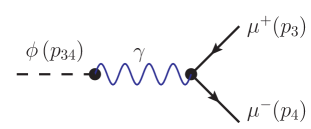
Figure 3: Decay of a $\phi$ meson to $\mu^{+}\mu^{-}$.

The decay rate $\phi\to\mu^{+}\mu^{-}$ is calculated from the diagram Fig. 3 (neglecting radiative corrections) as

$$\Gamma(\phi\to\mu^{+}\mu^{-})=\frac{1}{12\pi}\,|g_{\phi\to\mu^{+}\mu^{-}}|^{2}\,m_{\phi}\left(1+\frac{2m_{\mu}^{2}}{m_{\phi}^{2}}\right)\left(1-\frac{4m_{\mu}^{2}}{m_{\phi}^{2}}\right)^{1/2}\,.$$ (38)

From the experimental values Tanabashi:2018oca

$$m_{\phi}=(1019.461\pm 0.016)\;{\rm MeV}\,,$$

$$\Gamma(\phi\to\mu^{+}\mu^{-})/\Gamma_{\phi}=(2.86\pm 0.19)\times 10^{-4}\,,$$

$$\Gamma_{\phi}=(4.249\pm 0.013)\;{\rm MeV}\,,$$ (39)

we get

$$\Gamma(\phi\to\mu^{+}\mu^{-})=(1.21\pm 0.08)\times 10^{-3}\;{\rm MeV}$$ (40)

and using (38)

$$g_{\phi\mu^{+}\mu^{-}}=(6.71\pm 0.22)\times 10^{-3}\,.$$ (41)

On the other hand, using (37) directly with the standard range for $\gamma_{\phi}$ quoted in (3.24) of Ewerz:2013kda , $4\pi/\gamma_{\phi}^{2}=0.0716\pm 0.0017$, we get

$$g_{\phi\mu^{+}\mu^{-}}=(6.92\pm 0.08)\times 10^{-3}\,.$$ (42)

Within the errors the two values obtained in (41) and (42) are compatible. In the following we shall take (42) for our calculations.

IV Results

In this section we wish to present first results for three cases $pp\to pp\phi(1020)$, and with $\phi$ decaying to $K^{+}K^{-}$ or $\mu^{+}\mu^{-}$, corresponding to the processes discussed in Secs. II and III. For details how to calculate the subleading processes contributing to $pp\to pp(\phi\to K^{+}K^{-})$ we refer the reader to Appendix C.

IV.1 Comparison with the WA102 data

The $\phi$-meson production in central proton-proton collisions was studied by the WA102 Collaboration at $\sqrt{s}=29.1$ GeV. The experimental cross section quoted in Table 1 of Kirk:2000ws is

$$\sigma_{\rm exp}=(60\pm 21)\,\mathrm{nb}\,.$$ (43)

In Kirk:2000ws also the $\mathrm{dP_{t}}$ dependence of $\phi$ production and the distribution in $\phi_{pp}$ were presented. Here $\mathrm{dP_{t}}$ is the “glueball-filter variable” Close:1997pj ; Barberis:1996iq defined as:

$$\mbox{\boldmath$dP_{t}$}=\mbox{\boldmath$q_{t,1}$}-\mbox{\boldmath$q_{t,2}$}=\mbox{\boldmath$p_{t,2}$}-\mbox{\boldmath$p_{t,1}$}\,,\quad\mathrm{dP_{t}}=|\mbox{\boldmath$dP_{t}$}|\,,$$ (44)

and $\phi_{pp}$ is the azimuthal angle between the transverse momentum vectors $p_{t,1}$, $p_{t,2}$ of the outgoing protons. Both variables, $\mathrm{dP_{t}}$ and $\phi_{pp}$, are defined in the $pp$ center-of-mass frame. For the kinematics see e.g. Appendix D of Lebiedowicz:2013ika .

In Fig. 4 (left panel) we compare our theoretical predictions for the $\phi_{pp}$ distribution to the WA102 experimental data for the $pp\to pp\phi$ reaction normalised to the central value of the total cross section $\sigma_{\rm exp}=60$ nb from Kirk:2000ws ; see (43). We consider the two photoproduction contributions: $\gamma\mathbb{P}$ plus $\mathbb{P}\gamma$ and $\gamma\widetilde{M}$ plus $\widetilde{M}\gamma$ with $\widetilde{M}=\pi^{0},\eta$. We denote, for brevity, the coherent sum of the contributions $\gamma\mathbb{P}$ and $\mathbb{P}\gamma$ by $\gamma$-$\mathbb{P}$, the coherent sum of $\gamma\widetilde{M}$ and $\widetilde{M}\gamma$ by $\gamma$-$\widetilde{M}$. The analogous notation will be used for these and all other contributions in the following. For the photon-pomeron fusion we show the results for the two parameter sets, A and B, discussed in Appendix B (see Fig. 31). For the estimation of an upper limit of the $\gamma$-$\widetilde{M}$ contribution we take $\Lambda_{\widetilde{M}NN}=\Lambda_{\phi\gamma\widetilde{M}}=1.2$ GeV in (86) and (87); see the discussion and Fig. 32 in Appendix B. We find that the $\gamma$-$\widetilde{M}$ contribution is much smaller than the $\gamma$-$\mathbb{P}$ contribution. It constitutes about 15 $\%$ of $\gamma$-$\mathbb{P}$ in the integrated cross section. The $\gamma$-$S$ ($S=f_{0}(500)$, $f_{0}(980)$, $a_{0}(980)$) contribution terms are expected to be even smaller than the $\gamma$-$\widetilde{M}$ [$\widetilde{M}=\pi^{0}$, $\eta$] ones; see Fig. 32 in Appendix B. Therefore, we neglect the $\gamma$-$\widetilde{M}$- and $\gamma$-$S$-fusion contributions in the further considerations. Clearly, we see that the photoproduction mechanism is not enough to describe the WA102 data, at least if we take the central value of $\sigma_{\rm exp}$ quoted in (43) for normalising the data for the $\phi_{pp}$ distribution.

In Fig. 4 (right panel) we show the distributions in rapidity of the $\phi$ meson. The photoproduction mechanisms with $\mathbb{P}$ exchange ($\gamma\mathbb{P}$ and $\mathbb{P}\gamma$) dominate at midrapidity. The $\gamma\widetilde{M}$ and $\widetilde{M}\gamma$ components are separated and contribute in the backward and forward regions of ${\rm y}_{\phi}$, respectively. The separation in rapidity means also the lack of interference effects between the $\gamma\widetilde{M}$ and $\widetilde{M}\gamma$ components.

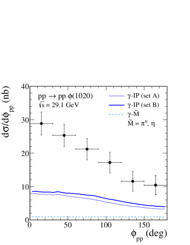
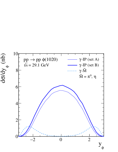
Figure 4: The distributions in $\phi_{pp}$ and in ${\rm y}_{\phi}$ for the $\phi$ photoproduction processes in the $pp\to pp\phi$ reaction at $\sqrt{s}=29.1$ GeV. The data points have been normalized to the central value for $\sigma_{\rm exp}$ (43) from Kirk:2000ws . The results for the photon-pomeron fusion are presented for the two parameter sets, set A and set B, as defined in Appendix B, see the caption of Fig. 31, (the bottom and top solid lines, respectively). We also show the contribution from the $\gamma$-$\widetilde{M}$ ($\widetilde{M}=\pi^{0},\eta$) fusion (the dashed lines). The absorption effects are included here.

It is a known fact that absorption effects due to strong proton-proton interactions have an influence on the shape of the distributions in $\phi_{pp}$, $\rm{dP_{t}}$, $|t_{1}|$ and $|t_{2}|$. Thus, absorption effects should be included in realistic calculations. In the calculations presented we have included the absorptive corrections in the one-channel eikonal approximation as was discussed, e.g., in Sec. 3.3 of Lebiedowicz:2014bea . The absorption effects lead to a large damping of the cross sections for purely hadronic diffractive processes and a relatively small reduction of the cross section for the photoproduction mechanism. We obtain the ratio of full and Born cross sections $\langle S^{2}\rangle$ (the gap survival factor) at $\sqrt{s}=29.1$ GeV and without any cuts included as follows $\langle S^{2}\rangle\cong 0.8$ for the photoproduction contribution and $\langle S^{2}\rangle\cong 0.4$ for the purely hadronic diffractive contributions discussed below. However, the absorption strongly depends on the kinematic cuts on $|t_{1}|$ and $|t_{2}|$. This will be discussed in detail when presenting our predictions for the LHC; see Sec. IV.2 below.

The question is now: what are the contributions to $\phi$ CEP which could fill the gap between the photoproduction result and the WA102 data in the left panel of Fig. 4? In the following we shall explore if this can be achieved by the subleading fusion processes $\omega$-$\mathbb{P}$, $\phi$-$\mathbb{P}$, $\omega$-$f_{2\mathbb{R}}$, and $\rho$-$\pi^{0}$ and/or the odderon-pomeron fusion giving a $\phi$ meson; see Appendix C and Sec. II.2, respectively.

In Fig. 5 we show results for the $\gamma$-$\mathbb{P}$ and the subleading fusion processes ($\omega$-$\mathbb{P}$, $\phi$-$\mathbb{P}$, $\omega$-$f_{2\mathbb{R}}$, and $\rho$-$\pi^{0}$). We present results for two approaches as follows. In the top panels (approach II) we show results for the reggeon-pomeron ($\phi_{\mathbb{R}}$-$\mathbb{P}$, $\omega_{\mathbb{R}}$-$\mathbb{P}$) and the reggeon-reggeon ($\omega_{\mathbb{R}}$-$f_{2\mathbb{R}}$) contributions, (107)–(111), and in the bottom panels (approach I) we show results for the reggeized-$\phi/\omega$-meson exchanges (100)–(106). The $\rho$-$\pi^{0}$ fusion contribution is calculated in the approach I, i.e., for the reggeized $\rho^{0}$-meson exchange.

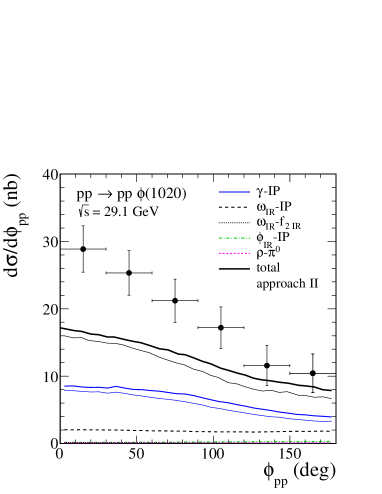
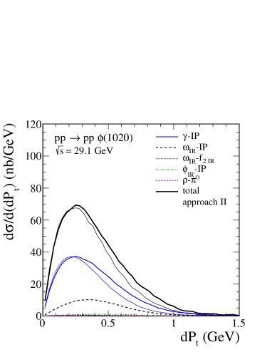
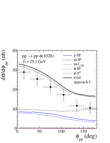
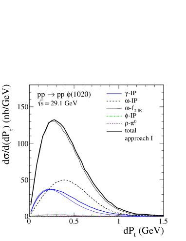
Figure 5: Distributions in proton-proton relative azimuthal angle $\phi_{pp}$ (left panels) and in $\rm{dP_{t}}$ (44), the “glueball filter” variable (right panels), for the $pp\to pp\phi$ reaction at $\sqrt{s}=29.1$ GeV. The data points have been normalized to the central value of the total cross section (43) from Kirk:2000ws . The results for the fusion processes $\gamma$-$\mathbb{P}$ (the two blue solid lines), $\omega$-$\mathbb{P}$ (the black dashed line), $\omega$-$f_{2\mathbb{R}}$ (the black dotted line), $\phi$-$\mathbb{P}$ (the green dash-dotted line), and $\rho$-$\pi^{0}$ (the violet dotted line) are presented. In the top panels the $\omega$-$\mathbb{P}$, $\phi$-$\mathbb{P}$ and $\omega$-$f_{2\mathbb{R}}$ exchanges are treated, respectively, as reggeon-pomeron and reggeon-reggeon exchanges (approach II) while in the bottom panels these contributions are calculated in the reggeized-vector-meson approach (101) (approach I). The coherent sum of these contributions is shown by the two black solid lines. The lower blue and black solid lines are for the parameter set A (72) and the upper lines are for the parameter set B (73) in the calculation of the $\gamma$-$\mathbb{P}$ fusion contribution. The absorption effects are included here.

In Figs. 6–7 we present several differential distributions for the $\gamma$-$\mathbb{P}$ and the $\mathbb{O}$-$\mathbb{P}$ fusion processes corresponding to the diagrams shown in Figs. 1 and 2, respectively, and for the subleading processes $\omega$-$\mathbb{P}$, $\phi$-$\mathbb{P}$, $\omega$-$f_{2\mathbb{R}}$ and $\rho$-$\pi^{0}$ fusion. In the panels (a) and (b) of Fig. 6 the $\omega$- and $\phi$-exchanges are treated as reggeon exchanges (approach II) while in the panel (c) as the reggeized-vector-meson exchange (101) (approach I). For the $\mathbb{O}$-$\mathbb{P}$ fusion contribution we take the following parameters, see (27)–(33),

$$\eta_{\mathbb{O}}=-1\,,\;\;\alpha_{\mathbb{O}}(0)=1.05\,,\;\;\alpha^{\prime}_{\mathbb{O}}=0.25\;\mathrm{GeV}^{-2}\,,$$ (45)

$$\Lambda_{0,\,\mathbb{P}\mathbb{O}\phi}^{2}=0.5\;{\rm GeV}^{2}\,,$$ (46)

and we choose different values for $a_{\mathbb{P}\mathbb{O}\phi}$ and $b_{\mathbb{P}\mathbb{O}\phi}$:

$${\rm(a)} a_{\mathbb{P}\mathbb{O}\phi}=-0.8\;{\rm GeV}^{-3}\,,\;\;b_{\mathbb{P}\mathbb{O}\phi}=1.0\;{\rm GeV}^{-1}\,;$$ (47)

$${\rm(b)} a_{\mathbb{P}\mathbb{O}\phi}=-0.8\;{\rm GeV}^{-3}\,,\;\;b_{\mathbb{P}\mathbb{O}\phi}=1.6\;{\rm GeV}^{-1}\,;$$ (48)

$${\rm(c)} a_{\mathbb{P}\mathbb{O}\phi}=-0.6\;{\rm GeV}^{-3}\,,\;\;b_{\mathbb{P}\mathbb{O}\phi}=1.6\;{\rm GeV}^{-1}\,.$$ (49)

The results shown in panels (a) and (b) of Fig. 6 correspond to the approach II and the $\mathbb{P}\mathbb{O}\phi$ parameters in (47) and (48), respectively. The results shown in panel (c) correspond to the approach I and (49). The coherent sum of all contributions is shown by the black solid lines. The lower line is for the parameter set A of photoproduction (72) and the upper line is for set B (73).

We have checked that these parameters are compatible with our analysis of the WA102 data for the $pp\to pp\phi\phi$ reaction discussed in Lebiedowicz:2019jru . Comparing the results shown in Fig. 5 with those in Fig. 6 we can see that the complete results indicate a large interference effect between the $\gamma$-$\mathbb{P}$, $\mathbb{O}$-$\mathbb{P}$, $\omega$-$\mathbb{P}$, $\omega$-$f_{2\mathbb{R}}$, and $\phi$-$\mathbb{P}$ terms.

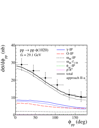
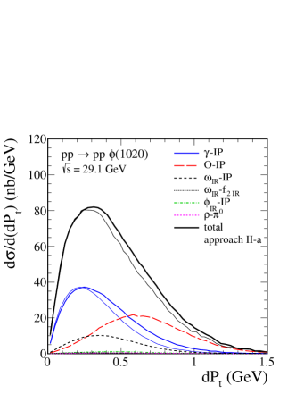
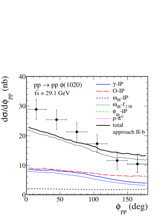
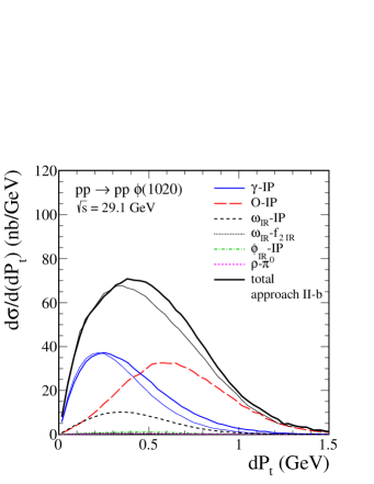
(a) (b) (c)

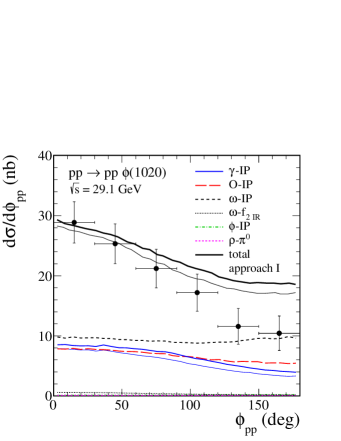
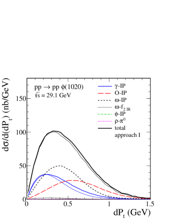
Figure 6: The $\phi_{pp}$ (left panels) and $\rm{dP_{t}}$ (right panels) distributions for the $pp\to pp\phi$ reaction at $\sqrt{s}=29.1$ GeV. The data points have been normalized to the central value of the total cross section (43) from Kirk:2000ws . The meaning of the lines is the same as in Fig. 5 but here we added the $\mathbb{O}$-$\mathbb{P}$ fusion term (see the red long-dashed line). The results shown in panels (a) and (b) correspond to the approach II and the $\mathbb{P}\mathbb{O}\phi$ parameters in (47) and (48), respectively. The results shown in panel (c) correspond to the approach I and (49). The coherent sum of all contributions is shown by the black solid lines. The lower line is for the parameter set A of photoproduction (72) and the upper line is for set B (73). The absorption effects are included here.

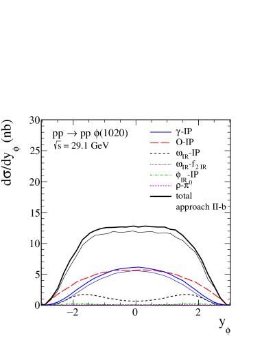
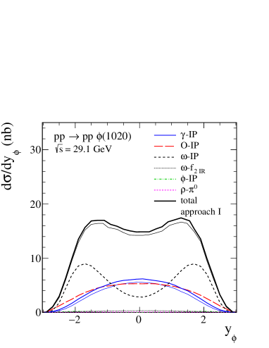
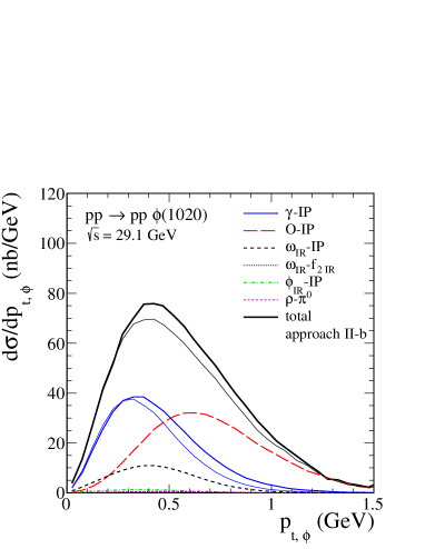
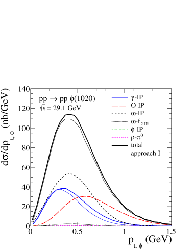
Figure 7: Distributions in rapidity of the $\phi$ meson (top panels) and in transverse momentum of the $\phi$ meson (bottom panels) for the $pp\to pp\phi$ reaction at $\sqrt{s}=29.1$ GeV. The meaning of the lines is the same as in Fig. 6.

In Kirk:2000ws experimental values for the cross sections in three $\mathrm{dP_{t}}$ intervals and for the ratio of $\phi$ production at small $\mathrm{dP_{t}}$ to large $\mathrm{dP_{t}}$ are given. We show our corresponding results in Table 1 for the two approaches, I and II, with appropriate $\mathbb{P}\mathbb{O}\phi$ coupling constants (47), (48), (49). Here we take the parameter set B (73) for the $\gamma$-$\mathbb{P}$ fusion contributions.

Now we discuss our results concerning the WA102 data. As already mentioned we find that the $\gamma$-$\mathbb{P}$ fusion processes alone cannot describe the WA102 data for the $\phi_{pp}$ distribution. This holds even if we scale down the experimental data by about 30 % corresponding to the quoted error on the total cross section in (43). Thus, we need other contributions, subleading ones or maybe odderon-pomeron fusion. From the subleading ones we find that the $\gamma$-$\pi^{0}$ and $\gamma$-$\eta$ contributions are very small; see Fig. 4. Also the $\rho$-$\pi^{0}$-fusion contribution turns out to be very small. According to our results, the important subleading contributions are $\omega$-$\mathbb{P}$, $\omega$-$f_{2\mathbb{R}}$ and $\phi$-$\mathbb{P}$ fusion. We have treated them with two methods of reggeization, I and II. The reggeized vector-meson approach I, see (101), (102), almost certainly overestimates these contributions. The reggeization means that we replace the vector-meson exchange by a coherent sum of exchanges with spin $1+3+5+...$. The higher the spin the higher the mass of the exchanged particle. In (101) this increase of mass is not taken into account leading to the overestimate. Also, the distribution in $\phi_{pp}$ in this approach I is too flat and does not fit the data; see the $\omega$-$\mathbb{P}$ contribution in the left bottom panel in Fig. 5. The approach II, on the other hand, assumes reggeon exchanges, $\omega_{\mathbb{R}}$ and $\phi_{\mathbb{R}}$. This approach maybe underestimates the contributions if $s_{1}$ or $s_{2}$ are small, but should be very reasonable for large $s_{1}$ or $s_{2}$. But note that in our reaction the threshold for $s_{1}$ and $s_{2}$ is already quite large $s_{\rm thr}\approx 4$ GeV²; see (103). We see clearly from Fig. 5 that in this approach the sum of the $\gamma$-$\mathbb{P}$, $\gamma$-$f_{2\mathbb{R}}$, $\omega_{\mathbb{R}}$-$\mathbb{P}$, $\omega_{\mathbb{R}}$-$f_{2\mathbb{R}}$, $\phi_{\mathbb{R}}$-$\mathbb{P}$ and $\rho$-$\pi^{0}$ contributions , added coherently, cannot explain the $\phi_{pp}$ data. This gives a hint that the missing contribution could be the odderon-pomeron fusion. And, indeed, with suitable odderon parameters we arrive at a decent description of the $\phi_{pp}$ and the $\rm{dP_{t}}$ data from WA102; see Fig. 6 and Table 1, respectively. However, we have to remember that the $\phi_{pp}$ distributions have a large normalisation uncertainty due to the relatively large error on $\sigma_{\rm exp}$ (43). Therefore, we emphasise that our fits to the WA102 data on single $\phi$ CEP only give a hint that this reaction could be very interesting for a search of odderon effects. It would be nice if we could fix the odderon contribution to $\phi$ CEP at the WA102 energy more quantitatively. But we must leave this to the experimentalists who know in detail the statistical and systematic errors of the data, including the error correlations. Also the theoretical uncertainties of the subleading contributions are relatively large at the WA102 energy. These latter uncertainties should, however, be much smaller at LHC energies. From Fig. 7 we see that the odderon-pomeron contribution dominates at larger $|{\rm y}_{\phi}|$ and $p_{t,\phi}$ compared to the photon-pomeron contribution. As we shall see this also holds at LHC energies and should help in searches for odderon effects there.

Table 1: Results of central $\phi$ production as a function of $\mathrm{dP_{t}}$ expressed as a percentage of its total contribution at the WA102 collision energy $\sqrt{s}=29.1$ GeV. In the last column the ratios of $\sigma(\mathrm{dP_{t}}\leqslant\,0.2~{}\mathrm{GeV})/\sigma(\mathrm{dP_{t}}\geqslant\,0.5~{}\mathrm{GeV})$ are given. The experimental numbers are from Table 2 of Kirk:2000ws . The theoretical numbers correspond to the total results including all terms contributing; see the upper black lines in the right panels of Figs. 5 and 6.

	$\mathrm{dP_{t}}\leqslant 0.2$ GeV	$0.2\leqslant\mathrm{dP_{t}}\leqslant 0.5$ GeV	$\mathrm{dP_{t}}\geqslant 0.5$ GeV	Ratio
experiment	$8\pm 3$	$47\pm 3$	$45\pm 4$	$0.18\pm 0.07$
approach II, no odderon	22.0	46.9	31.1	0.71
approach I, no odderon	19.5	48.0	32.5	0.60
approach II-a	17.4	42.2	40.4	0.43
approach II-b	13.3	37.0	49.7	0.27
approach I	14.7	41.1	44.2	0.33

IV.2 Predictions for the LHC experiments

IV.2.1 The $pp\to ppK^{+}K^{-}$ reaction

In this subsection we wish to show our predictions for the LHC experiments. We start with the presentation of the differential distributions for the $pp\to pp(\phi\to K^{+}K^{-})$ reaction (3) which we integrate in the $\phi$ resonance region (2). First we show, for orientation purposes, results for the $\gamma\mathbb{P}$- and the $\mathbb{O}\mathbb{P}$-fusion contributions separately (see the diagrams shown in Figs. 1 and 2, respectively). For the final results we shall, of course, add these contributions coherently and calculate absorption corrections at the amplitude level. We have checked that in the kinematic regimes discussed in the following the subleading contributions (see Appendix C) can be safely neglected.

In Figs. 8–16 we show the results for $\sqrt{s}=13$ TeV, and $|\eta_{K}|<2.5$, $p_{t,K}>0.1$ GeV and sometimes with extra cuts on the leading protons of 0.17 GeV $<|p_{y,1}|,|p_{y,2}|<$ 0.50 GeV as will be the proton momentum window for the ALFA detectors placed on both sides of the ATLAS detector. The choice of such cuts is based on the analysis initiated by the ATLAS Collaboration; see Sikora_poster . For comparison, we will also show our predictions for the ATLAS-ALFA experiment for $p_{t,K}>0.2$ GeV; see Figs. 15–17 and Table 2 below.

Figure 8 shows the Born-level distributions in $|t_{1}|$ (top panels) and in transverse momentum $p_{t,1}=|\mbox{\boldmath$p_{t,1}$}|$ of the proton $p\,(p_{1})$ (bottom panels). In the left panels the photoproduction contributions are plotted while in the right panels we show the results for the odderon contributions. The results for the parameter set B (73) for the photoproduction term and for the parameters quoted in (45), (46), (48) for the $\mathbb{O}$-$\mathbb{P}$ fusion are presented. We show results for two diagrams separately and for their coherent sum (denoted by “total”). The interference effects between the two diagrams are clearly visible, especially for the $\mathbb{O}$-$\mathbb{P}$-fusion mechanism. A different behaviour is seen at small $|t_{1}|$ for the $\gamma\mathbb{P}$ and the $\mathbb{O}\mathbb{P}$ components. Due to the photon exchange the protons are scattered only at small angles and the $\gamma\mathbb{P}$ distribution has a singularity for $|t_{1}|\to 0$. Of course, $t_{1}=0$ cannot be reached here from kinematics. In contrast, the $\mathbb{O}\mathbb{P}$ distribution shows a dip for $|t_{1}|\to 0$. The explanation of this type of behaviour is given in Appendix C of Bolz:2014mya . In the bottom panels we show the $p_{t}$ distributions for proton $p\,(p_{1})$. Here these differences are also clearly visible.

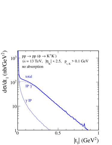
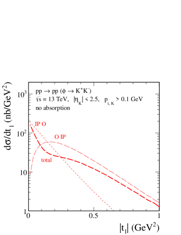
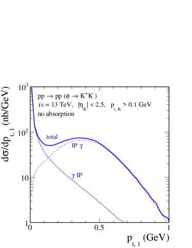
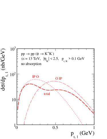
Figure 8: The distributions in four-momentum transfer squared $|t_{1}|$ (top panels) and in transverse momentum $p_{t,1}$ of the proton $p\,(p_{1})$ (bottom panels) for the $pp\to pp(\phi\to K^{+}K^{-})$ reaction at $\sqrt{s}=13$ TeV and for $|\eta_{K}|<2.5$, $p_{t,K}>0.1$ GeV. Absorption effects are not included here. In the left panels we show the results for the photoproduction mechanism obtained with the parameter set B (73). The results for the $\gamma\mathbb{P}$- and $\mathbb{P}\gamma$-fusion contributions are presented. Their coherent sum is shown by the blue solid thick line. In the right panels we present the results for the odderon-pomeron-fusion mechanism obtained with the parameters quoted in (45), (46), and (48). Again, we show the $\mathbb{O}\mathbb{P}$- and $\mathbb{P}\mathbb{O}$-fusion contributions separately and their coherent sum (red long-dashed thick line).

In Fig. 9 we show results for the hadronic diffractive contribution for the two types of couplings in the $\mathbb{P}\mathbb{O}\phi$ vertex (32) separately and when both couplings are taken into account. The distributions in $\phi_{pp}$, the relative azimuthal angle between the outgoing protons, in $\rm{y_{diff}}=\rm{y}_{3}-\rm{y}_{4}$, the rapidity distance between the two centrally produced kaons, and in $\phi_{K^{+},\,{\rm CS}}$ and $\cos\theta_{K^{+},\,{\rm CS}}$ where the azimuthal and polar angles of the $K^{+}$ meson are defined in the Collins-Soper (CS) frame, see Appendix D, are presented. We can see that the complete result indicates a large interference effect of the $a_{\mathbb{P}\mathbb{O}\phi}$ and $b_{\mathbb{P}\mathbb{O}\phi}$ coupling contributions in the amplitudes. Note, in particular, that both the $a$ and the $b$ term separately give a $\cos\theta_{K^{+},\,{\rm CS}}$ distribution with a maximum at $\cos\theta_{K^{+},\,{\rm CS}}=0$. On the contrary, their coherent sum has a minimum there.

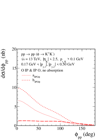
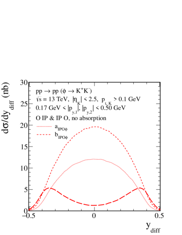
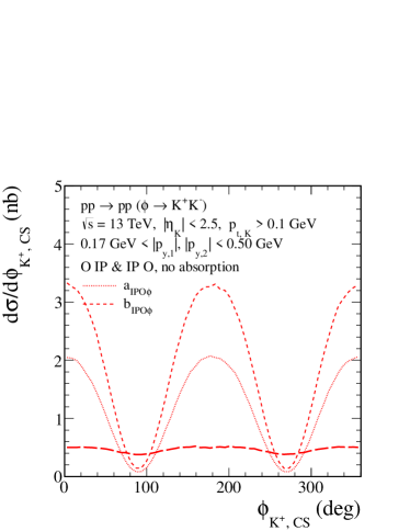
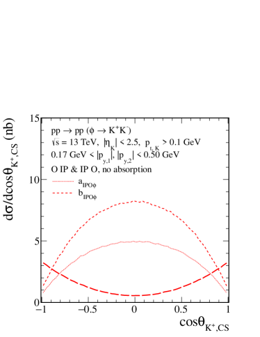
Figure 9: The differential cross sections for $\sqrt{s}=13$ TeV and for the ATLAS-ALFA cuts ($|\eta_{K}|<2.5$, $p_{t,K}>0.1$ GeV, 0.17 GeV $<|p_{y,1}|,|p_{y,2}|<$ 0.50 GeV). We present the results for the hadronic diffractive contribution neglecting absorption effects. The thick long-dashed line represents the complete result with both $a_{\mathbb{P}\mathbb{O}\phi}$ and $b_{\mathbb{P}\mathbb{O}\phi}$ couplings (48) included in the amplitude; see the $\mathbb{P}\mathbb{O}\phi$ vertex (32). The contributions for the two type of couplings, $a$ and $b$ from (48), are shown separately: the dotted line corresponds to the calculation only with $a_{\mathbb{P}\mathbb{O}\phi}$, and the short-dashed line corresponds to the calculation only with $b_{\mathbb{P}\mathbb{O}\phi}$.

Figure 10 shows the differential cross sections $d\sigma/d\phi_{pp}$ (see the top panels) and $d\sigma/d\rm{y_{diff}}$ (see the bottom panels) without (the left panels) and with (the right panels) limitations on the leading protons. The blue lines correspond to the photoproduction contributions while the red lines to the hadronic diffractive contributions. The thin lines represent the results for one of the two diagrams separately ($\gamma\mathbb{P}$ or $\mathbb{P}\gamma$ as well as $\mathbb{O}\mathbb{P}$ or $\mathbb{P}\mathbb{O}$) and the thick lines represent their coherent sum ($\gamma\mathbb{P}$ plus $\mathbb{P}\gamma$, $\mathbb{O}\mathbb{P}$ plus $\mathbb{P}\mathbb{O}$). The reader is asked to note a reversed interference behaviour for the photon-pomeron and odderon-pomeron mechanisms. The influence of kinematic cuts on the leading protons is also shown. We see that due to the cuts on the leading protons (0.17 GeV $<|p_{y,1}|,|p_{y,2}|<$ 0.50 GeV) the photoproduction term is strongly suppressed. The odderon-pomeron contribution dominates at larger $|\rm{y_{diff}}|$ compared to the photon-pomeron contribution.

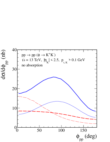
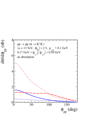
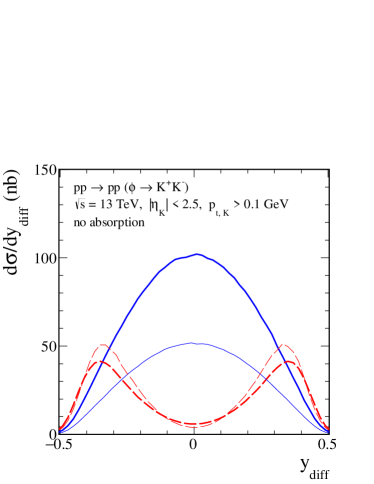
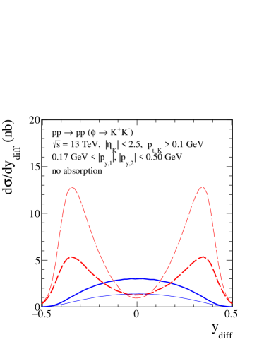
Figure 10: The distributions in azimuthal angle $\phi_{pp}$ between the transverse momentum vectors $p_{t,1}$, $p_{t,2}$ of the outgoing protons (top panels) and in rapidity difference between kaons $\mathrm{y_{diff}}$ (bottom panels). The calculations were performed for $\sqrt{s}=13$ TeV and for the ATLAS-ALFA experimental cuts $|\eta_{K}|<2.5$, $p_{t,K}>0.1$ GeV (left panels), and with extra cuts on the leading protons of 0.17 GeV $<|p_{y,1}|,|p_{y,2}|<$ 0.50 GeV (right panels). The blue thick solid line corresponds to the coherent sum of the two diagrams ($\gamma\mathbb{P}$ and $\mathbb{P}\gamma$). The red thick dashed line corresponds to the coherent sum of the $\mathbb{O}\mathbb{P}$ and $\mathbb{P}\mathbb{O}$ contributions. The thin lines correspond to the results for one of the two diagrams separately (the second contribution is the same). For the $\gamma$-$\mathbb{P}$-fusion contribution we take the parameter set B (73). For the $\mathbb{O}$-$\mathbb{P}$-fusion contribution we take the parameters quoted in (45), (46), and (48).

In Fig. 11 we show the kaon angular distributions in the $K^{+}K^{-}$ rest system using the Collins-Soper (CS) frame; see Appendix D. The Collins-Soper frame which we use here is defined as in our recent paper on extracting the $\mathbb{P}\mathbb{P}f_{2}(1270)$ couplings in the $pp\to pp\pi^{+}\pi^{-}$ reaction Lebiedowicz:2019por with $K^{+}$ and $K^{-}$ in the place of $\pi^{+}$ and $\pi^{-}$, respectively. For the $pp\to pp(\phi\to K^{+}K^{-})$ reaction we can observe interesting structures in the $\phi_{K^{+},\,{\rm CS}}$ (top panel) and in the $\cos\theta_{K^{+},\,{\rm CS}}$ (bottom panel) distributions. The distributions in $\phi_{K^{+},\,{\rm CS}}$ for the hadronic diffractive contribution ($\mathbb{O}\mathbb{P}$ plus $\mathbb{P}\mathbb{O}$) are relatively flat. The photoproduction term, in contrast, shows pronounced maxima and minima which are due to the interference of the $\gamma\mathbb{P}$ and $\mathbb{P}\gamma$ terms. The cuts on leading protons considerably change the shape of the $\phi_{K^{+},\,{\rm CS}}$ distributions for the photon-exchange contribution. The angular distribution $d\sigma/d\cos\theta_{K^{+},\,{\rm CS}}$ looks promising for a search of odderon effects as it is very different for the $\gamma$-$\mathbb{P}$- and the $\mathbb{O}$-$\mathbb{P}$-fusion processes.

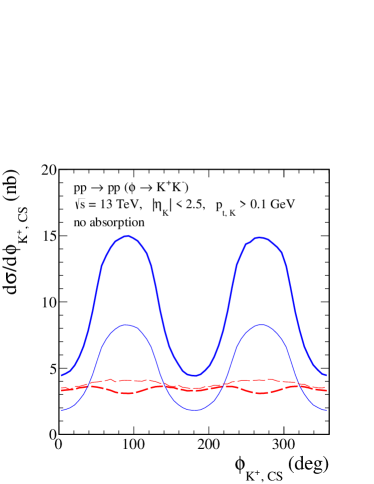
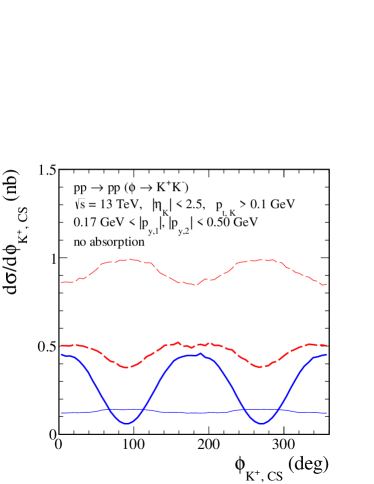
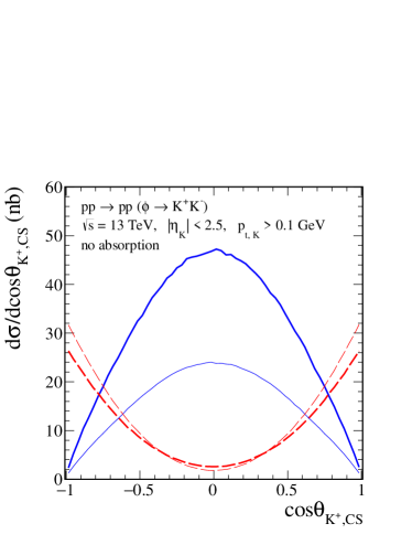
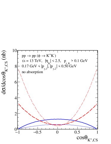
Figure 11: The distributions in $\phi_{K^{+},{\rm CS}}$ (top panel) and in $\cos\theta_{K^{+},\,{\rm CS}}$ (bottom panel) for $\sqrt{s}=13$ TeV, $|\eta_{K}|<2.5$, $p_{t,K}>0.1$ GeV (left panels), and with extra cuts on the leading protons of 0.17 GeV $<|p_{y,1}|,|p_{y,2}|<$ 0.50 GeV (right panels). The meaning of the lines is the same as in Fig. 10.

In Fig. 12 we compare results without (the thin lines) and with (the thick lines) absorption effects. The absorption effects have been included in our analysis within the one-channel-eikonal approach. For the ATLAS-ALFA kinematics the absorption effects lead to a large damping of the cross sections both for the hadronic diffractive and for the photoproduction mechanisms. We find a suppression factor of the cross section of $\langle S^{2}\rangle\simeq 0.3$; see Table 2. A similar value of suppression was found in Ryutin:2019khx (see Fig. 14 there) for the exclusive $pp\to pp\pi^{+}\pi^{-}$ reaction for the diffractive continuum process at the LHC energy. From Fig. 12 we see that the absorption effects also modify the shape of the distributions.

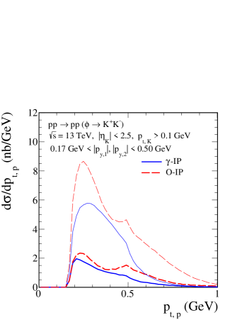
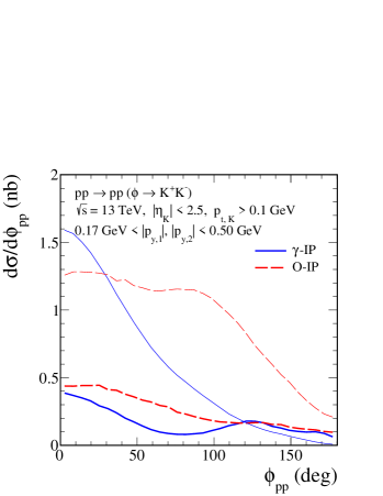
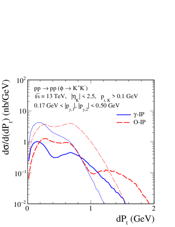
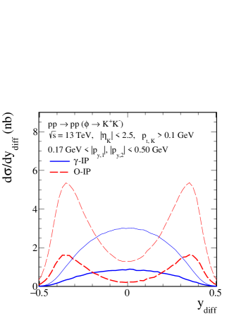
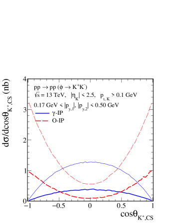
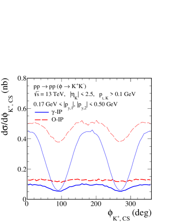
Figure 12: The differential cross sections for $\sqrt{s}=13$ TeV and the ATLAS-ALFA cuts without (the thin lines) and with (the thick lines) absorption effects. For the $\gamma$-$\mathbb{P}$-fusion contribution we take the parameter set B (73). For the $\mathbb{O}$-$\mathbb{P}$-fusion contribution we take the parameters quoted in (45), (46), and (48).

From the $\cos\theta_{K^{+},\,{\rm CS}}$ distributions shown in Figs. 11 and 12 we can conclude that from the $\gamma$-$\mathbb{P}$ fusion the $\phi$ meson gets preferentially a transverse polarisation giving a distribution proportional to $\sin^{2}\theta_{K^{+},\,{\rm CS}}$. For the $\mathbb{O}$-$\mathbb{P}$ fusion, on the other hand, we find that the $\phi$ meson gets preferentially a longitudinal polarisation with a distribution proportional to $\cos^{2}\theta_{K^{+},\,{\rm CS}}$. This different behaviour can be understood using again the considerations of Appendix C of Bolz:2014mya . The $\gamma$-$\mathbb{P}$ contribution is largest for very small $|t|$, see Fig. 8, where the virtual photon has essentially only transverse polarisation which it will transmit to the $\phi$. The $\mathbb{O}$-$\mathbb{P}$ fusion, on the other hand, gives a very small contribution for very small $|t|$. For larger $|t|$, however, where the odderon contributes most, the longitudinal cross section has a “large” factor $|t|$ relative to the transverse term. (This is quite analogous to what happens in DIS for the standard cross sections of the absorption of the virtual photon on the proton, $\sigma_{T}$ and $\sigma_{L}$. For $Q^{2}\to 0$ $\sigma_{T}$ goes to a constant, $\sigma_{L}$ is proportional to $Q^{2}$; see for instance Britzger:2019lvc ).

Up to now we have shown results including the ATLAS-ALFA experimental cuts for a concrete set of parameters, set B (73) for the photoproduction term and (48) for the $\mathbb{P}\mathbb{O}\phi$ coupling parameters. In Fig.  13 we show results for different parameter sets, as discussed in Sec. IV.1, for the $\gamma$-$\mathbb{P}$- and $\mathbb{O}$-$\mathbb{P}$-fusion processes. The upper blue solid line is for the parameter set B of photoproduction (73) and the lower blue solid line is for set A (72). The red long-dashed line corresponds to the odderon parameters quoted in (45), (46), and the $\mathbb{P}\mathbb{O}\phi$ coupling parameters (b) (48), the red dash-dotted line is for the choice of $\mathbb{P}\mathbb{O}\phi$ coupling parameters (a) (47), and the red dotted line is for (49).

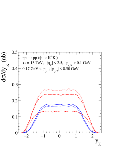
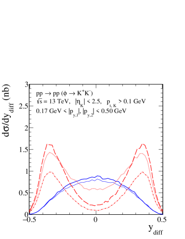
Figure 13: Results for the ATLAS-ALFA experiment at $\sqrt{s}=13$ TeV. The lower blue solid line represents the result for the parameter set A of photoproduction (72) and the upper line is for set B (73). The red long-dashed line represents the odderon-pomeron fusion with the parameters quoted in (45), (46), and the $\mathbb{P}\mathbb{O}\phi$ coupling parameters (48). the red dash-dotted line is for the choice (47) of the $\mathbb{P}\mathbb{O}\phi$ coupling parameters, and the red dotted line is for (49). The absorption effects are included here.

In Figs. 14, 15 and 16 we show distributions in several variables for the ATLAS-ALFA experimental cuts, $\sqrt{s}=13$ TeV, $|\eta_{K}|<2.5$, 0.17 GeV $<|p_{y,1}|,|p_{y,2}|<$ 0.50 GeV, $p_{t,K}>0.1$ GeV and $p_{t,K}>0.2$ GeV. The absorption effects are included in the calculations. We show results for the $\gamma$-$\mathbb{P}$- and $\mathbb{O}$-$\mathbb{P}$-fusion contributions separately (see the blue and red lines, respectively) and when both terms are added coherently at the amplitude level (the black lines). We take for the $\gamma$-$\mathbb{P}$- and $\mathbb{O}$-$\mathbb{P}$-fusion contributions the coupling parameters (73) and (48), respectively. In Fig. 17 we show the results for (47) $a_{\mathbb{P}\mathbb{O}\phi}=-0.8\;{\rm GeV}^{-3}$ and $b_{\mathbb{P}\mathbb{O}\phi}=1.0\;{\rm GeV}^{-1}$ [instead of $b_{\mathbb{P}\mathbb{O}\phi}=1.6\;{\rm GeV}^{-1}$ (48)]. We can see that the complete result indicates a large interference effect of $\gamma$-$\mathbb{P}$- and $\mathbb{O}$-$\mathbb{P}$-fusion terms. The odderon-pomeron contribution dominates clearly at larger $|\rm{y_{diff}}|$, $p_{t,K^{+}K^{-}}$, the transverse momentum of the $K^{+}K^{-}$ pair, and $\cos\theta_{K^{+},\,{\rm CS}}=\pm 1$, compared to the photon-pomeron contribution. We encourage the experimentalists associated to the ATLAS-ALFA experiment to prepare such distributions, especially $d\sigma/d\rm{y_{diff}}$, $d\sigma/d\cos\theta_{K^{+},\,{\rm CS}}$, and $d\sigma/d\phi_{K^{+},\,{\rm CS}}$. Observation of the pattern of maxima and minima would be interesting by itself as it is due to interference effects. Note, in particular, the different pattern of $\phi_{K^{+},\,{\rm CS}}$ distributions in Figs. 16 and 17. Within the same kinematic cuts we can observe for $\phi_{K^{+},\,{\rm CS}}=0,\pi,2\pi$ destructive interference for (48) and constructive interference for (47). The same is clearly seen also for $\cos\theta_{K^{+},\,{\rm CS}}=0$.

It is worth adding that much smaller interference effects are predicted when no cuts on the outgoing protons are required; see the results in Table 2 and Figs. 19, 20 below. When cuts on transverse momenta of the outgoing protons are imposed then the $\gamma$-$\mathbb{P}$- and $\mathbb{O}$-$\mathbb{P}$-fusion contributions become comparable and large interference effects are in principle possible.

We have checked numerically that for $\alpha_{\mathbb{O}}(0)=1.0$, instead of $\alpha_{\mathbb{O}}(0)=1.05$ [see (30)], we get a bit smaller cross section for the $\mathbb{O}$-$\mathbb{P}$-fusion contribution but the shape of the differential distributions (e.g., $d\sigma/d\phi_{pp}$, $d\sigma/dt_{1,2}$) is not changed. In our plots for the LHC energies we have taken mainly the odderon coupling parameters from (48). This is to be understood as an example. For the parameters from (47) the odderon effects at the LHC are typically smaller than those from (48) by a factor of roughly 2; see Figs. 13, 15, 17. Figures 15 and 17 show distinct interference effects between the $\gamma$-$\mathbb{P}$- and $\mathbb{O}$-$\mathbb{P}$-fusion contributions which depend on the choice of the odderon coupling parameters. In an experimental analysis of single $\phi$ CEP at the LHC clearly the odderon parameters from (29) and (32) should be considered as fit parameters to be determined from the comparison of our theoretical results with the data.

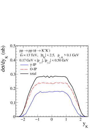
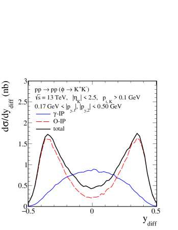
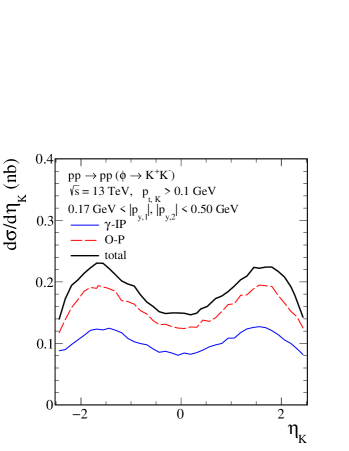
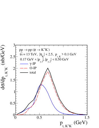
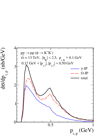
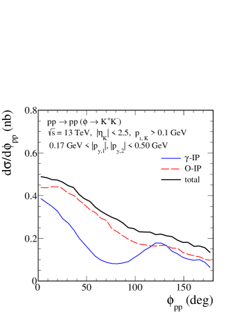
Figure 14: Selected predictions for the ATLAS-ALFA experiment at $\sqrt{s}=13$ TeV. The absorption effects are included here. The blue solid line represents the result for the photoproduction mechanism for set B (73) while the red long-dashed line represents the odderon-pomeron fusion with the parameters quoted in (45), (46), and the $\mathbb{P}\mathbb{O}\phi$ coupling parameters (48). The coherent sum of the two fusion processes is shown by the black solid line.

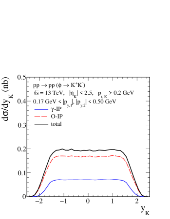
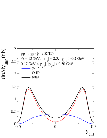
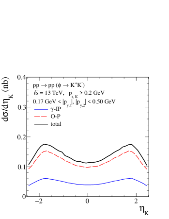
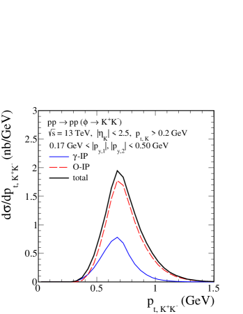
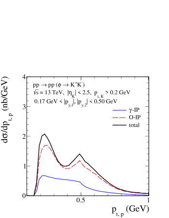
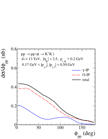
Figure 15: The same as in Fig. 14 but for $p_{t,K}>0.2$ GeV.

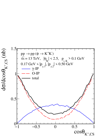
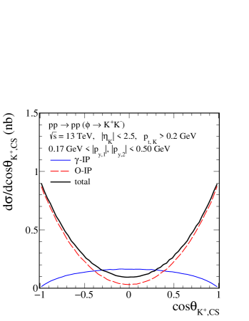
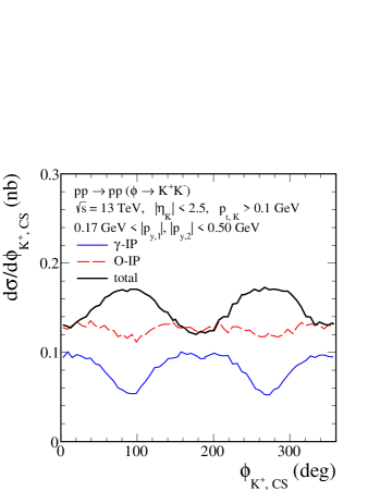
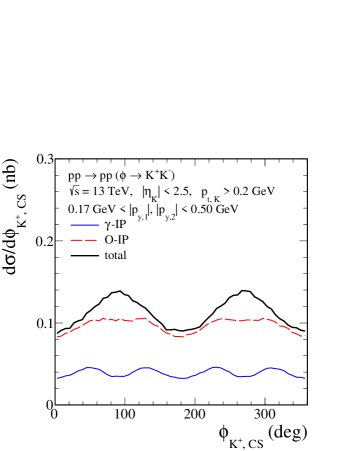
Figure 16: The distributions in $\cos\theta_{K^{+},\,{\rm CS}}$ (the top panels) and in $\phi_{K^{+},\,{\rm CS}}$ (the bottom panels). The calculations were performed for $\sqrt{s}=13$ TeV and for the ATLAS-ALFA experimental cuts $|\eta_{K}|<2.5$, $p_{t,K}>0.1$ GeV (left panels) or $p_{t,K}>0.2$ GeV (right panels), and with extra cuts on the leading protons of 0.17 GeV $<|p_{y,1}|,|p_{y,2}|<$ 0.50 GeV. The meaning of the lines is the same as in Fig. 14. The absorption effects are included here.

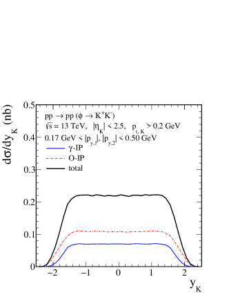
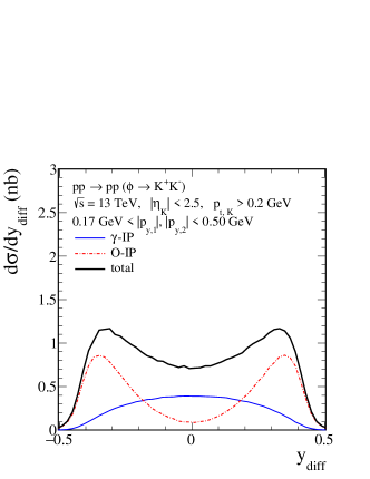
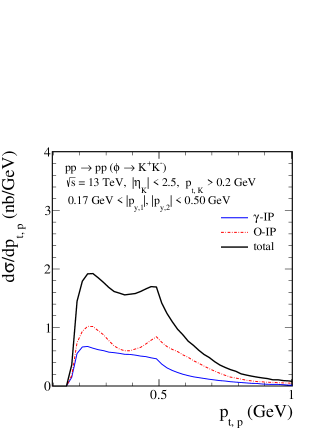
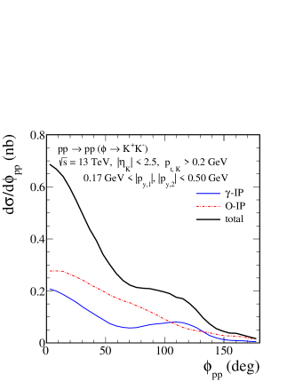
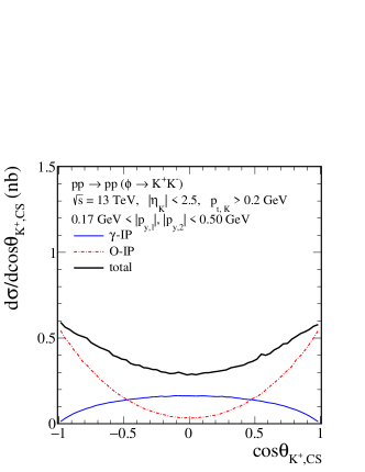
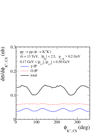
Figure 17: The differential cross sections for the $pp\to pp(\phi\to K^{+}K^{-})$ reaction calculated for $\sqrt{s}=13$ TeV and for the ATLAS-ALFA experimental cuts $|\eta_{K}|<2.5$, $p_{t,K}>0.2$ GeV, 0.17 GeV $<|p_{y,1}|,|p_{y,2}|<$ 0.50 GeV. The meaning of the lines is the same as in Fig. 14 but here we have taken the smaller value of the $b_{\mathbb{P}\mathbb{O}\phi}$ coupling parameter; see (47). The absorption effects are included here.

Now we shall discuss results for the LHCb experimental conditions. In Fig. 18 we show the two-dimensional distributions in ($p_{t,K^{+}}$, $p_{t,K^{-}}$) for $\sqrt{s}=13$ TeV, $2.0<\eta_{K}<4.5$, and $p_{t,K}>0.1$ GeV. In the left panel we show the result for $\gamma$-$\mathbb{P}$ fusion obtained with the parameter set B (73). In the right panel we show the result for $\mathbb{O}$-$\mathbb{P}$ fusion for the parameters quoted in (45), (46), and (48). We can see that the $\gamma$-$\mathbb{P}$-fusion contribution is larger at smaller $p_{t,K}$ than the $\mathbb{O}$-$\mathbb{P}$-fusion contribution. Therefore, a low-$p_{t,K}$ cut on transverse momenta of the kaons can be helpful to reduce the $\gamma$-$\mathbb{P}$-fusion contribution; compare the left and right panels in Figs. 19 and 20 below.

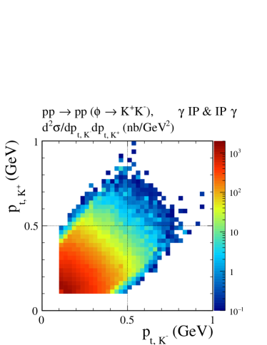
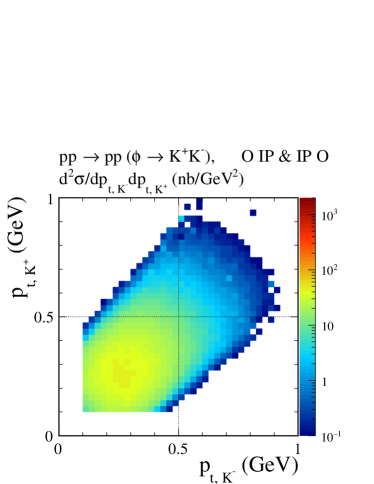
Figure 18: The two-dimensional distributions in ($p_{t,K^{+}}$, $p_{t,K^{-}}$) for the $pp\to pp(\phi\to K^{+}K^{-})$ reaction via $\gamma$-$\mathbb{P}$-fusion (left panel) and via $\mathbb{O}$-$\mathbb{P}$-fusion (right panel) processes. The calculations were done for $\sqrt{s}=13$ TeV and with cuts on $2.0<\eta_{K}<4.5$ and $p_{t,K}>0.1$ GeV. Here we show the result for $\gamma$-$\mathbb{P}$ fusion obtained with the parameter set B (73) while the result for $\mathbb{O}$-$\mathbb{P}$ fusion was obtained with the parameters quoted in (45), (46), and (48). The absorption effects are included here.

In Figs. 19 and 20 we show several distributions for $\gamma$-$\mathbb{P}$- and $\mathbb{O}$-$\mathbb{P}$-fusion contributions and their coherent sum for the LHCb experimental conditions, $\sqrt{s}=13$ TeV, $2.0<\eta_{K}<4.5$, $p_{t,K}>0.3$ GeV (left panels) or $p_{t,K}>0.5$ GeV (right panels). The absorption effects were included in the calculations. For larger kaon transverse momenta (or transverse momentum of the $K^{+}K^{-}$ pair) the odderon-exchange contribution, using our parameters for the odderon, is bigger than the photon-exchange one.

As in the previous (ATLAS-ALFA) case the angular distributions in the $K^{+}K^{-}$ Collins-Soper rest system seem interesting. In Fig. 21 we show the two-dimensional distributions in ($\phi_{K^{+},\,{\rm CS}}$, $\cos\theta_{K^{+},\,{\rm CS}}$) for $2.0<\eta_{K}<4.5$ and $p_{t,K}>0.3$ GeV. We see here again that the $\gamma$-$\mathbb{P}$ fusion leads predominantly to transverse polarisation of the $\phi$ meson. The distribution for the $\mathbb{O}$-$\mathbb{P}$ fusion (the right panel of Fig. 21) shows clearly a strong longitudinal $\phi$-meson component but, due to the marked $\phi_{K^{+},\,{\rm CS}}$ dependence, also transverse $\phi$ components must be present.

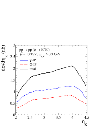
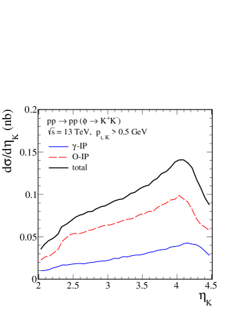
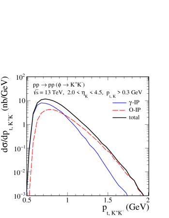
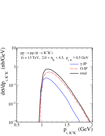
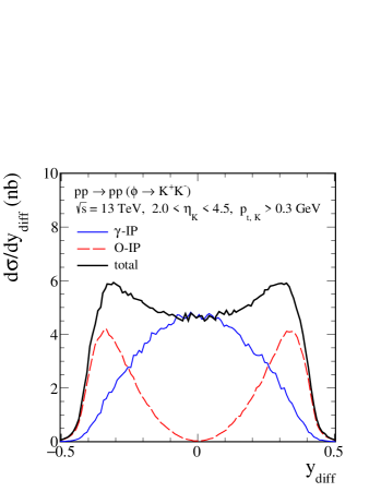
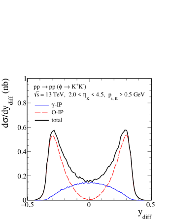
Figure 19: The differential cross sections for the $pp\to pp(\phi\to K^{+}K^{-})$ reaction. Calculations were done for $\sqrt{s}=13$ TeV, $2.0<\eta_{K}<4.5$, and $p_{t,K}>0.3$ GeV (left panels) or $p_{t,K}>0.5$ GeV (right panels). The meaning of the lines is the same as in Fig. 14. Results for the photoproduction (blue solid lines) and the $\mathbb{O}$-$\mathbb{P}$-fusion (red lines) contributions are shown separately. The black solid line corresponds to the coherent sum of the $\gamma$-$\mathbb{P}$- and $\mathbb{O}$-$\mathbb{P}$-fusion processes with the coupling parameters (73) and (48), respectively. The absorption effects are included here.

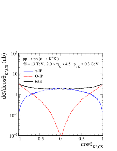
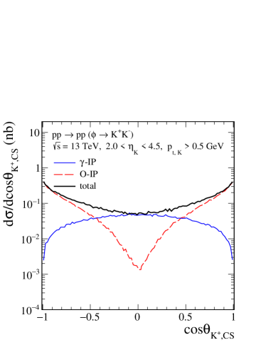
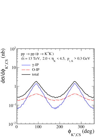
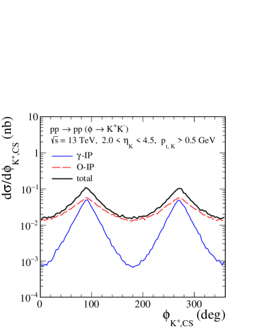
Figure 20: The distributions in $\cos\theta_{K^{+},\,{\rm CS}}$ and $\phi_{K^{+},\,{\rm CS}}$ for the same experimental cuts as in Fig. 19. Also the meaning of the lines is as in Fig. 19.

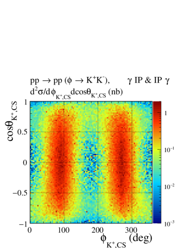
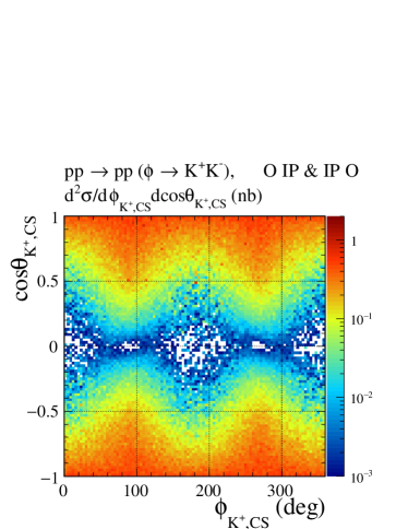
Figure 21: The two-dimensional distributions in ($\phi_{K^{+},\,{\rm CS}}$, $\cos\theta_{K^{+},\,{\rm CS}}$) for the $pp\to pp(\phi\to K^{+}K^{-})$ reaction via $\gamma$-$\mathbb{P}$ fusion (left panel) and via $\mathbb{O}$-$\mathbb{P}$ fusion (right panel). The calculations were done for $\sqrt{s}=13$ TeV and with the cuts $2.0<\eta_{K}<4.5$ and $p_{t,K}>0.3$ GeV. We show the result for $\gamma$-$\mathbb{P}$ fusion obtained with the parameter set B (73) while the result for $\mathbb{O}$-$\mathbb{P}$ fusion was obtained with the parameters quoted in (45), (46), and (48). The absorption effects are included here.

IV.2.2 The $pp\to pp\mu^{+}\mu^{-}$ reaction

The $\phi$ meson can also be observed in the $\mu^{+}\mu^{-}$ channel. In this subsection we wish to show our predictions for the $pp\to pp\mu^{+}\mu^{-}$ reaction for the LHCb experiment at $\sqrt{s}=13$ TeV for the $2.0<\eta_{\mu}<4.5$ pseudorapidity range. Here we require no detection of the leading protons.

In Fig. 22 we present the $\mu^{+}\mu^{-}$ invariant mass distributions in the $\phi(1020)$ resonance region. We show the contributions from the $\gamma$-$\mathbb{P}$- and $\mathbb{O}$-$\mathbb{P}$-fusion processes and the continuum $\gamma\gamma\to\mu^{+}\mu^{-}$ term. The dimuon-continuum process ($\gamma\gamma\to\mu^{+}\mu^{-}$) was discussed, e.g., in Lebiedowicz:2018muq in the context of the ATLAS measurement Aaboud:2017oiq . In our analysis here we are looking at the dimuon invariant mass region $M_{\mu^{+}\mu^{-}}\in(1.01,1.03)$ GeV.

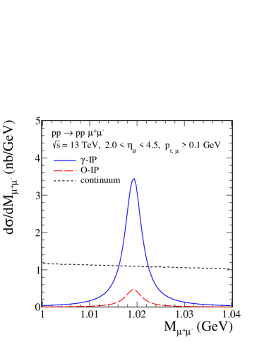
Figure 22: The distributions in $\mu^{+}\mu^{-}$ invariant mass for the exclusive $pp\to pp\mu^{+}\mu^{-}$ reaction including the $\phi$-meson production via the $\gamma$-$\mathbb{P}$- and the $\mathbb{O}$-$\mathbb{P}$-fusion processes and the nonresonant $\gamma\gamma\to\mu^{+}\mu^{-}$ continuum term. The calculations were done for $\sqrt{s}=13$ TeV, $2.0<\eta_{\mu}<4.5$, and $p_{t,\mu}>0.1$ GeV. Here we show the result for $\gamma$-$\mathbb{P}$ fusion (the blue solid line) obtained with the parameter set B (73). The result for $\mathbb{O}$-$\mathbb{P}$ fusion (the red long-dashed line) was obtained with the parameters quoted in (45), (46), and (48). The black short-dashed line corresponds to the continuum contribution. The absorption effects are included here.

Note, that in the continuum term, $\gamma\gamma\to\mu^{+}\mu^{-}$, the $\mu^{+}\mu^{-}$ are in a state of charge conjugation $C=+1$. For $\phi\to\mu^{+}\mu^{-}$ we have a state of $C=-1$. Thus, the interference of the continuum and the $\phi$-production reactions will lead to $\mu^{+}$-$\mu^{-}$ asymmetries. We have checked, however, that the interference in the $\mu^{+}\mu^{-}$ channel is smaller than our numerical precision, definitely smaller than 2%.

In Fig. 23 we show two-dimensional distributions in ($p_{t,\mu^{+}}$, $p_{t,\mu^{-}}$) for three different processes. The result in the panel (a) corresponds to the continuum contribution without the cut on $M_{\mu^{+}\mu^{-}}$. Here the maximum of the cross section is placed along the $p_{t,\mu^{+}}=p_{t,\mu^{-}}$ line which is due to the predominantly small transverse momenta of the photons in this photon-exchange process. The results in the panels (b), (c), and (d) correspond to the continuum term, the $\gamma$-$\mathbb{P}$- and $\mathbb{O}$-$\mathbb{P}$-fusion processes, respectively, including the limitation on $M_{\mu^{+}\mu^{-}}$.

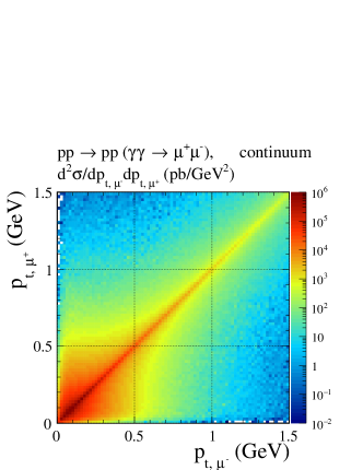
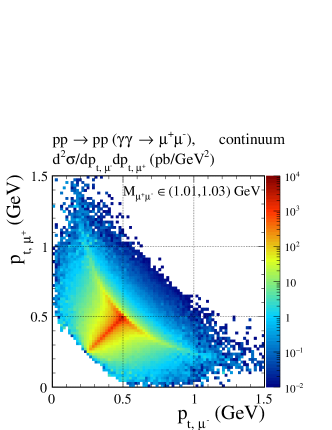
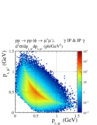
(a) (b) (c) (d)

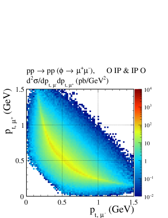
Figure 23: The two-dimensional distributions in ($p_{t,\mu^{+}}$, $p_{t,\mu^{-}}$) for the $pp\to pp\mu^{+}\mu^{-}$ reaction. The calculations were done for $\sqrt{s}=13$ TeV and $2.0<\eta_{\mu}<4.5$. The results in the panels (a) and (b) correspond to the $\mu^{+}\mu^{-}$ continuum without and with the cut on $M_{\mu^{+}\mu^{-}}\in(1.01,1.03)$ GeV, respectively. The results in the panels (c) and (d) correspond to the $\phi$ production via $\gamma$-$\mathbb{P}$ fusion and via $\mathbb{O}$-$\mathbb{P}$ fusion, respectively. No absorption effects are included here.

In Figs. 24 and 25, we show the predictions for the $pp\to pp\mu^{+}\mu^{-}$ reaction for typical experimental lower cuts on the transverse momentum of the muons, $p_{t,\mu}>0.1$ GeV and $p_{t,\mu}>0.5$ GeV, respectively. In contrast to dikaon production here there is for both the $\gamma$-$\mathbb{P}$- and the $\mathbb{O}$-$\mathbb{P}$-fusion contributions a maximum at $\rm{y_{diff}}=0$ (or $\cos\theta_{\mu^{+},{\rm CS}}=0$). In Fig. 24 the continuum contribution is large. Imposing a larger cut on the transverse momenta of the muons reduces the continuum contribution which, however, still remains sizeable at $\rm{y_{diff}}=0$. Such a cut reduces the statistics of the measurement; see the results in Table 2. In Fig. 25 we show our predictions for different choices of parameters. The $\mu^{+}\mu^{-}$ channel seems to be less promising in identifying the odderon exchange at least when only the $p_{t,\mu}$ cuts are imposed. Eventually, the absolute normalization of the cross section and detailed studies of shapes of distributions should provide a clear answer whether one can observe the odderon-exchange mechanism here.

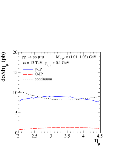
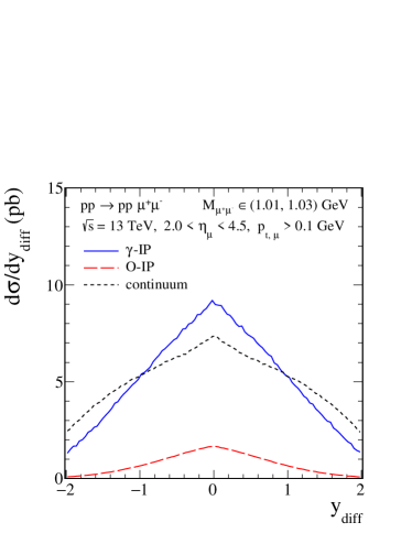
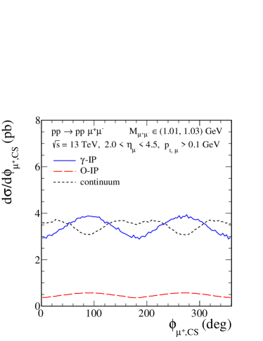
Figure 24: The differential cross sections for the $pp\to pp\mu^{+}\mu^{-}$ reaction in the dimuon invariant mass region $M_{\mu^{+}\mu^{-}}\in(1.01,1.03)$ GeV. Calculations were done for $\sqrt{s}=13$ TeV, $2.0<\eta_{\mu}<4.5$, and $p_{t,\mu}>0.1$ GeV. The meaning of the lines is the same as in Fig. 22. We take the $\gamma$-$\mathbb{P}$- and $\mathbb{O}$-$\mathbb{P}$-fusion contributions for the coupling parameters (73) and (48), respectively. The absorption effects are included here.

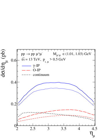
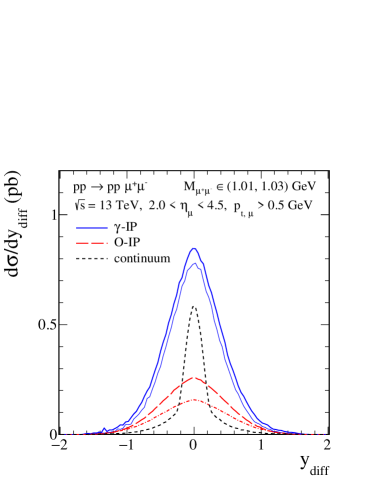
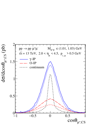
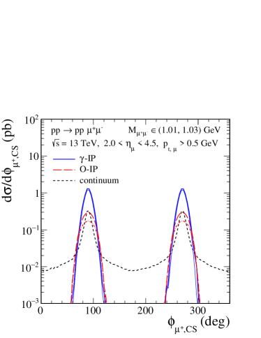
Figure 25: The same as in Fig. 24 but for $p_{t,\mu}>0.5$ GeV. The upper blue solid line is for the $\gamma$-$\mathbb{P}$-fusion contribution for the parameter set B (73) while the lower blue solid line is for set A (72). The red long-dashed line corresponds to the $\mathbb{O}$-$\mathbb{P}$-fusion contribution with the parameters quoted in (45), (46), and (48), the red dash-dotted line is for another choice of the $\mathbb{P}\mathbb{O}\phi$ coupling parameter (47). The black short-dashed line corresponds to the continuum contribution. The absorption effects are included here.

In Fig. 26 we present the distributions in transverse momentum of the $\mu^{+}\mu^{-}$ pair. We can see that the low-$p_{t,\mu^{+}\mu^{-}}$ cut can be helpful to reduce the continuum ($\gamma\gamma\to\mu^{+}\mu^{-}$) and photon-pomeron-fusion contributions.

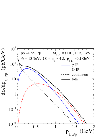
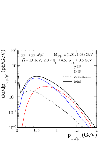
Figure 26: The distributions in transverse momentum of the $\mu^{+}\mu^{-}$ pair for the $pp\to pp\mu^{+}\mu^{-}$ reaction in the dimuon invariant mass region $M_{\mu^{+}\mu^{-}}\in(1.01,1.03)$ GeV. Calculations were done for $\sqrt{s}=13$ TeV, $2.0<\eta_{\mu}<4.5$ and for $p_{t,\mu}>0.1$ GeV (left panel) and for $p_{t,\mu}>0.5$ GeV (right panel). The meaning of the lines is the same as in Fig. 22 but here we added the coherent sum of all contributions shown by the black solid line. Here we take the $\gamma$-$\mathbb{P}$- and $\mathbb{O}$-$\mathbb{P}$-fusion contributions for the coupling parameters (73) and (48), respectively. The absorption effects are included here.

In Fig. 27 we show the results when imposing in addition a cut $p_{t,\mu^{+}\mu^{-}}>0.8$ GeV. The $\gamma\gamma\to\mu^{+}\mu^{-}$ contribution is now very small. We can see from the $\rm{y_{diff}}$ distribution that the photon-pomeron term gives a broader distribution than the odderon-pomeron term. At $\rm{y_{diff}}=0$ the odderon-exchange term is now bigger than the photoproduction terms.

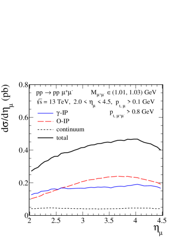
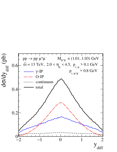
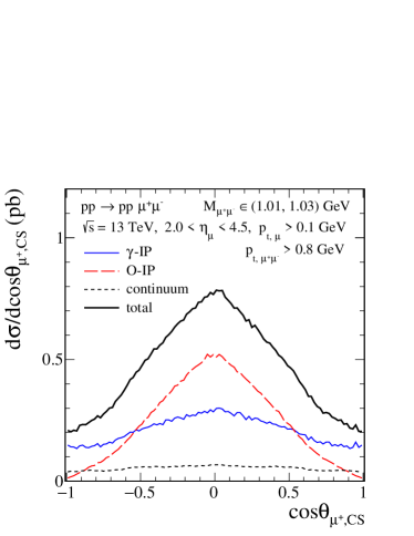
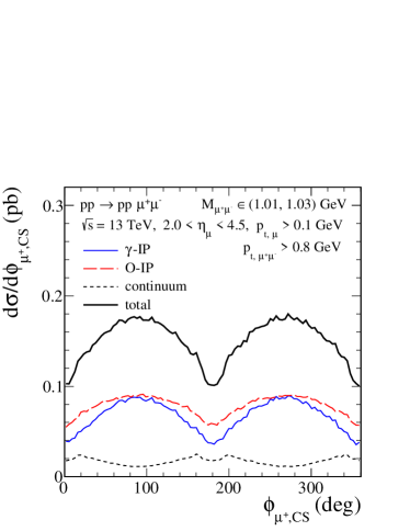
Figure 27: The differential cross sections for the $pp\to pp\mu^{+}\mu^{-}$ reaction in the dimuon invariant mass region $M_{\mu^{+}\mu^{-}}\in(1.01,1.03)$ GeV. Calculations were done for $\sqrt{s}=13$ TeV, $2.0<\eta_{\mu}<4.5$, $p_{t,\mu}>0.1$ GeV, and $p_{t,\mu^{+}\mu^{-}}>0.8$ GeV. The meaning of the lines is the same as in Fig. 26. The absorption effects are included here.

In Table 2 we have collected integrated cross sections in nb for $\sqrt{s}=13$ TeV and with different experimental cuts for the exclusive $pp\to ppK^{+}K^{-}$ and $pp\to pp\mu^{+}\mu^{-}$ reactions including the $\gamma$-$\mathbb{P}$- and $\mathbb{O}$-$\mathbb{P}$-fusion processes separately. We also show the results for the coherent sum of the $\gamma$-$\mathbb{P}$- and $\mathbb{O}$-$\mathbb{P}$-fusion processes including absorption corrections. Here we take for the $\gamma$-$\mathbb{P}$- and $\mathbb{O}$-$\mathbb{P}$-fusion contributions the coupling parameters (73) and (48), respectively. The ratios of full and Born cross sections $\langle S^{2}\rangle$ (the gap survival factors) are also presented. We obtain $\langle S^{2}\rangle\simeq 0.2-0.3$ for the purely diffractive $\mathbb{O}$-$\mathbb{P}$ contribution. For the $\gamma$-$\mathbb{P}$ contribution we find that $\langle S^{2}\rangle$ strongly depends on the cuts on the leading protons.

Table 2: The integrated cross sections in nb for the central exclusive production of single $\phi$ mesons in proton-proton collisions with the subsequent decays $\phi\to K^{+}K^{-}$ or $\phi\to\mu^{+}\mu^{-}$. The results have been calculated for $\sqrt{s}=13$ TeV in the dikaon/dimuon invariant mass region $M_{34}\in(1.01,1.03)$ GeV and for some typical experimental cuts. We show results for the $\gamma$-$\mathbb{P}$- and $\mathbb{O}$-$\mathbb{P}$-fusion contributions separately and for their coherent sum (“total”). The ratios of full and Born cross sections $\langle S^{2}\rangle$ (the gap survival factors) are shown in the last column.

Cuts	Contributions	$\sigma^{(\rm{Born})}$ (nb)	$\sigma^{(\rm{full})}$ (nb)	$\langle S^{2}\rangle$
$|\eta_{K}|<2.5$, $p_{t,K}>0.1$ GeV	$\gamma$-$\mathbb{P}$	60.07	55.09	0.9
	$\mathbb{O}$-$\mathbb{P}$	21.40	6.44	0.3
	total		58.58
$|\eta_{K}|<2.5$, $p_{t,K}>0.1$ GeV,	$\gamma$-$\mathbb{P}$	1.77	0.52	0.3
0.17 GeV $<|p_{y,1}|,|p_{y,2}|<0.5$ GeV	$\mathbb{O}$-$\mathbb{P}$	2.91	0.79	0.3
	total		0.93
$|\eta_{K}|<2.5$, $p_{t,K}>0.2$ GeV,	$\gamma$-$\mathbb{P}$	1.07	0.24	0.2
0.17 GeV $<|p_{y,1}|,|p_{y,2}|<0.5$ GeV	$\mathbb{O}$-$\mathbb{P}$	2.10	0.61	0.3
	total		0.70
$|\eta_{K}|<2.5$, $p_{t,K}>0.5$ GeV,	$\gamma$-$\mathbb{P}$	$6.74\times 10^{-3}$	$0.76\times 10^{-3}$	0.1
0.17 GeV $<|p_{y,1}|,|p_{y,2}|<0.5$ GeV	$\mathbb{O}$-$\mathbb{P}$	$87.94\times 10^{-3}$	$18.97\times 10^{-3}$	0.2
	total		$20.47\times 10^{-3}$
$2.0<\eta_{K}<4.5$, $p_{t,K}>0.1$ GeV	$\gamma$-$\mathbb{P}$	43.18	40.07	0.9
	$\mathbb{O}$-$\mathbb{P}$	16.73	4.70	0.3
	total		43.28
$2.0<\eta_{K}<4.5$, $p_{t,K}>0.3$ GeV	$\gamma$-$\mathbb{P}$	3.09	2.57	0.8
	$\mathbb{O}$-$\mathbb{P}$	6.57	1.64	0.3
	total		4.24
$2.0<\eta_{K}<4.5$, $p_{t,K}>0.5$ GeV	$\gamma$-$\mathbb{P}$	$\;\,0.93\times 10^{-1}$	$\;\,0.66\times 10^{-1}$	0.7
	$\mathbb{O}$-$\mathbb{P}$	0.88	0.16	0.2
	total		0.24
$2.0<\eta_{\mu}<4.5$, $p_{t,\mu}>0.1$ GeV	$\gamma$-$\mathbb{P}$	$23.93\times 10^{-3}$	$20.96\times 10^{-3}$	0.9
	$\mathbb{O}$-$\mathbb{P}$	$10.06\times 10^{-3}$	$\;\,3.02\times 10^{-3}$	0.3
	total		$21.64\times 10^{-3}$
$2.0<\eta_{\mu}<4.5$, $p_{t,\mu}>0.5$ GeV	$\gamma$-$\mathbb{P}$	$\;\,1.21\times 10^{-3}$	$\;\,0.85\times 10^{-3}$	0.7
	$\mathbb{O}$-$\mathbb{P}$	$\;\,1.49\times 10^{-3}$	$\;\,0.45\times 10^{-3}$	0.2
	total		$\;\,1.07\times 10^{-3}$
$2.0<\eta_{\mu}<4.5$, $p_{t,\mu}>0.1$ GeV,	$\gamma$-$\mathbb{P}$	$\;\,0.70\times 10^{-3}$	$\;\,0.41\times 10^{-3}$	0.6
$p_{t,\mu^{+}\mu^{-}}>0.8$ GeV	$\mathbb{O}$-$\mathbb{P}$	$\;\,2.46\times 10^{-3}$	$\;\,0.51\times 10^{-3}$	0.2
	total		$\;\,0.91\times 10^{-3}$

We close this section with a brief comment on the absorptive corrections in the nonperturbative (soft) diffractive and in pQCD processes.

The survival factor for the soft exclusive process $pp\to pp\pi^{+}\pi^{-}$ via the pomeron-pomeron fusion for $\sqrt{s}=7$ TeV was calculated also in Ryutin:2019khx . From Fig. 14 of Ryutin:2019khx we see that the survival factor (only the $pp$ rescattering corrections) is about $\langle S^{2}\rangle=0.2$.

In the perturbative case there is an additional factor for the gluon-gluon fusion vertex. This factor suppresses the emission of virtual “soft” gluons that could fill rapidity gaps (Sudakov-like suppression). For “hard” pQCD processes at the LHC energies the expected $\langle S^{2}\rangle$ value is about 0.03 (or smaller); see, e.g., Petrov:2007kn ; Ryskin:2009tk ; Harland-Lang:2013dia . Besides the effect of eikonal screening, there is some suppression caused by the rescatterings of the protons with the intermediate partons (inside the unintegrated gluon distribution). This effect, neglected in the present calculations, is described by the so-called enhanced reggeon diagrams and usually denoted as $S^{2}_{\rm enh}$. The precise size of this effect is uncertain, but due to the relatively large transverse momentum (and so smaller absorptive cross section) of the intermediate partons, it is only expected to reduce the corresponding CEP cross section by a factor of at most a “few”, that is a much weaker suppression than in the case of $\langle S^{2}\rangle$, the eikonal survival factor; see, e.g., Ryskin:2009tk ; Harland-Lang:2013dia .

A similar method of calculation of the soft survival factor, $\langle S^{2}\rangle$, as in our paper, was used in the GRANITTI Monte Carlo event generator Mieskolainen:2019jpv . For instance, for central exclusive $\pi^{+}\pi^{-}$ production (via pomeron-pomeron fusion), denoted in Table 1 of Mieskolainen:2019jpv by $\pi^{+}\pi^{-}_{EL}$, the author gets $\langle S^{2}\rangle\simeq 0.2$ at the LHC energies. Note, that a much smaller $\langle S^{2}\rangle=0.06$ is obtained in Mieskolainen:2019jpv for a pQCD process, production of a gluon pair $gg$ at $\sqrt{s}=13$ TeV, using the pQCD based Durham model.

Finally, we note that for the $\gamma\gamma$-fusion processes the values of $\langle S^{2}\rangle$ also depend on kinematic regions considered; see, e.g., Lebiedowicz:2018muq .

V Conclusions

In the present paper we have discussed the possibility to search for odderon exchange in the $pp\to pp\phi$ reaction with the $\phi$ meson observed in the $K^{+}K^{-}$ or $\mu^{+}\mu^{-}$ channels. There are two basic processes: the relatively well known (at the Born level) photon-pomeron fusion and the rather elusive odderon-pomeron fusion. In our previous analysis on two $\phi$-meson production in proton-proton collisions Lebiedowicz:2019jru we tried to tentatively (optimistically) fix the parameters of the pomeron-odderon-$\phi$ vertex to describe the relatively large $\phi\phi$ invariant mass distribution measured by the WA102 Collaboration Barberis:1998bq . The calculation for the $pp\to pp\phi$ process requires in addition knowledge of the rather poorly known coupling of the odderon to the proton. The latter can be fixed, in principle, by a careful study of elastic proton-proton scattering. The present estimates suggest $\beta_{\mathbb{O}pp}\simeq 0.1\,\beta_{\mathbb{P}NN}$ [see Eq. (31)]. In the present study we therefore fixed the odderon coupling to the proton at this reasonable value and tried to make predictions for central exclusive $\phi$-meson production. Our results also depend on the assumptions made for the Regge trajectory of the odderon, Eqs. (29) and (30). In this context the photon-pomeron fusion is a background for the odderon-pomeron fusion. The parameters of photoproduction were fixed to describe the HERA $\phi$-meson photoproduction data; see Appendices A and B. There, we pay special attention to the importance of the $\phi$-$\omega$ mixing effect in the description of the $\gamma p\to\phi p$ and $\gamma p\to\omega p$ reactions. We would like to invite experimentalists to perform further studies of these reactions both with still unanalysed HERA data and data from ultraperipheral $Ap$ collisions. This should include $\omega$ and $\phi$ polarisation studies in order to get precise values for the relevant coupling parameters defined in Appendices A and B. To fix the parameters of the pomeron-odderon-$\phi$ vertex (coupling constants and cutoff parameters) we have considered several subleading contributions and compared our theoretical predictions for the $pp\to pp\phi$ reaction with the WA102 experimental data from Kirk:2000ws .

Having fixed the parameters of the model we have made estimates of the integrated cross sections as well as shown several differential distributions for $pp\to pp\phi$ at the WA102 energy $\sqrt{s}=29.1$ GeV. In addition we have discussed in detail exclusive production of single $\phi$ mesons at the LHC, both in the $K^{+}K^{-}$ and $\mu^{+}\mu^{-}$ observation channels, for two possible distinct types of measurements: (a) at midrapidity and without or with forward measurement of protons (relevant for ATLAS-ALFA or CMS-TOTEM), (b) at forward rapidities and without measurement of protons (relevant for LHCb). In contrast to low energies, where several processes may compete, at the large LHC energies the odderon-exchange contribution competes only with the photoproduction mechanism. We have considered different dedicated observables. Some of them seem to be promising. The distributions in $\rm{y_{diff}}$ (rapidity difference between kaons) and the angular distributions of kaons in the Collins-Soper frame seem particularly interesting for the $K^{+}K^{-}$ final state. These angular distributions give information on the polarisation state of the produced $\phi$ meson. It is a main result of our paper that, according to our odderon model, the polarisation of the $\phi$ and, as a consequence, the angular distribution of the kaons in the Collins-Soper frame are very different for the $\gamma$-$\mathbb{P}$- and $\mathbb{O}$-$\mathbb{P}$-fusion processes. This should be a big asset for an odderon search. Increasing the value of the cut on the transverse momenta of kaons improves the signal (pomeron-odderon fusion) to the background (photon-pomeron fusion) ratio. Of course, in this way the rates are reduced; see Table 2. In general, the $\mu^{+}\mu^{-}$ channel seems to be less promising in identifying the odderon exchange. In this case detailed studies of shapes of $d\sigma/d\rm{y_{diff}}$ or/and $d\sigma/d\cos\theta_{\mu^{+},{\rm CS}}$ would be very useful in understanding the general situation. To observe a sizeable deviation from photoproduction a $p_{t,\mu^{+}\mu^{-}}>0.8$ GeV cut on the transverse momentum of the $\mu^{+}\mu^{-}$ pair seems necessary. Such a cut reduces then the statistics of the measurement considerably. A combined analysis of both the $K^{+}K^{-}$ and the $\mu^{+}\mu^{-}$ channels should be the ultimate goal in searches for odderon exchange. We are looking forward to first experimental results on single $\phi$ CEP at the LHC.

In summary, we have presented results for single $\phi$ CEP both at the Born level as well as including absorption effects in the eikonal approximation. We have argued that the WA102 experimental results at c.m. energy $\sqrt{s}=29.1$ GeV leave room for a possible odderon-exchange contribution there. Then we have turned to LHC energies where single $\phi$ CEP can be studied by experiments such as: ATLAS-ALFA, CMS-TOTEM, ALICE, and LHCb. Using our results it should be possible to see experimentally if odderon effects as calculated are present, if our odderon parameters have to be changed, or if it is only possible to derive limits on the odderon parameters. We are looking forward also to relevant data from the lower energy COMPASS experiment. At high energies the deviations from the $\gamma$-$\mathbb{P}$-fusion contribution can be treated as a signal of odderon exchange. In our opinion several distributions should be studied to draw a definite conclusion on the odderon exchange. So far the odderon exchange was not unambiguously identified in any reaction. In the present paper we have shown that for the odderon search the study of central exclusive production of single $\phi$ mesons is a valuable addition and alternative to the study of elastic proton-proton scattering or production of two $\phi$ mesons in the $pp\to pp\phi\phi$ reaction discussed by us very recently; see Lebiedowicz:2019jru . But the results of our paper are not limited to the odderon search. We give in the Appendices A and B also all the necessary formulas for the analyses of $\omega$ and $\phi$ photoproduction in the framework of our tensor-pomeron model. We hope that experimentalists will perform such analysis using both data from HERA and from ultraperipheral $Ap$ collisions at the LHC. Such results will then be very useful to make refined predictions for $\phi$ CEP via the $\gamma$-$\mathbb{P}$ fusion. This process is not only a background for an odderon search but also interesting by itself.

Appendix A Off-diagonal diffractive $\omega\to\phi$ transition

In the naive quark model the nucleon has no $s\bar{s}$ content, whereas the $\phi$ meson is a pure $s\bar{s}$ state (ideal mixing of the vector mesons). Thus, the coupling of the $\phi$ meson to the nucleon is expected to be very weak. In practice there is a slight deviation from ideal mixing of the vector mesons, which means that the $\phi$ meson has a small $u\bar{u}+d\bar{d}$ component. Therefore, one should worry about diffractive off-diagonal $\omega\to\phi$ transitions ($\omega$ strongly couples to the nucleon). We should consider the diagrams shown below in Fig. 34. How to treat the off-diagonal diffractive transitions due to pomeron exchange?

The physical states $\omega$ and $\phi$ are usually written in terms of flavour eigenstates $\omega_{1}$ and $\omega_{8}$ and the so-called mixing angle $\theta_{V}$ [see (B1) of Titov:1999eu ]

$$\omega = \omega_{8}\cos\theta_{V}+\omega_{1}\sin\theta_{V}\,,$$

$$-\phi = -\omega_{8}\sin\theta_{V}+\omega_{1}\cos\theta_{V}\,,$$ (50)

where $\omega_{1}=\frac{1}{\sqrt{3}}\left(u\bar{u}+d\bar{d}+s\bar{s}\right)$, $\omega_{8}=\frac{1}{\sqrt{6}}\left(u\bar{u}+d\bar{d}-2s\bar{s}\right)$. The mixing angle can be written as:

$$\theta_{V}=\theta_{V,i}-\Delta\theta_{V}\;.$$ (51)

The first component corresponds to the so-called ideal mixing angle and the second one quantifies the deviation from the ideal mixing. For the ideal mixing angle $\theta_{V,i}$ we have :

$$\sin\theta_{V,i}=\sqrt{\frac{2}{3}}\,,\quad\cos\theta_{V,i}=\frac{1}{\sqrt{3}}\,,\quad\tan\theta_{V,i}=\sqrt{2}\,,\quad\theta_{V,i}=54.74^{\circ}\,.$$ (52)

Then it is easy to show, using (51) and (52), that:

$$\sin\theta_{V} = \sqrt{\frac{2}{3}}\cos\Delta\theta_{V}-\frac{1}{\sqrt{3}}\sin\Delta\theta_{V}\,,$$

$$\cos\theta_{V} = \frac{1}{\sqrt{3}}\cos\Delta\theta_{V}+\sqrt{\frac{2}{3}}\sin\Delta\theta_{V}\,.$$ (53)

Inserting this in (50) and defining $\omega_{0}=\frac{1}{\sqrt{2}}\left(u\bar{u}+d\bar{d}\right)$ and $\phi_{0}=-s\bar{s}$ the mixing equation reads:

$$\omega = \omega_{0}\cos(\Delta\theta_{V})+\phi_{0}\sin(\Delta\theta_{V})\,,$$

$$\phi = -\omega_{0}\sin(\Delta\theta_{V})+\phi_{0}\cos(\Delta\theta_{V})\,.$$ (54)

The reverse reads

$$\omega_{0} = \omega\cos(\Delta\theta_{V})-\phi\sin(\Delta\theta_{V})\,,$$

$$\phi_{0} = \omega\sin(\Delta\theta_{V})+\phi\cos(\Delta\theta_{V})\,.$$ (55)

It is well known that experimentally the angle $\Delta\theta_{V}$ is small. Thus, the physical $\omega$ and $\phi$ are nearly equal to $\omega_{0}$ and $\phi_{0}$, respectively.

Now we consider the $\mathbb{P}\omega_{\mathbb{R}}\omega$, $\mathbb{P}\omega_{\mathbb{R}}\phi$, $\mathbb{P}\phi_{\mathbb{R}}\omega$, and $\mathbb{P}\phi_{\mathbb{R}}\phi$ vertices for which we assume a structure as in (12) with appropriate coupling constants $a$ and $b$. In our case (CEP of $\phi$ meson in proton-proton collisions) the $\omega_{\mathbb{R}}$ ($\omega$ reggeon) is, however, off-mass shell and we neglect the rather unknown mixing in this Regge-like state and include mixing in the on-shell $\phi$ only. We shall argue, therefore, that in the $\mathbb{P}\omega_{\mathbb{R}}\omega$ and $\mathbb{P}\omega_{\mathbb{R}}\phi$ vertices only the $\omega_{0}$ will couple. In this way we get for our coupling constants $a$ and $b$

$$a_{\mathbb{P}\omega_{\mathbb{R}}\omega} = a_{\mathbb{P}\omega_{\mathbb{R}}\omega_{0}}\cos(\Delta\theta_{V})\,,$$

$$b_{\mathbb{P}\omega_{\mathbb{R}}\omega} = b_{\mathbb{P}\omega_{\mathbb{R}}\omega_{0}}\cos(\Delta\theta_{V})\,;$$ (56)

$$a_{\mathbb{P}\omega_{\mathbb{R}}\phi} = -a_{\mathbb{P}\omega_{\mathbb{R}}\omega_{0}}\sin(\Delta\theta_{V})\,,$$

$$b_{\mathbb{P}\omega_{\mathbb{R}}\phi} = -b_{\mathbb{P}\omega_{\mathbb{R}}\omega_{0}}\sin(\Delta\theta_{V})\,;$$ (57)

$$\frac{a_{\mathbb{P}\omega_{\mathbb{R}}\phi}}{a_{\mathbb{P}\omega_{\mathbb{R}}\omega}} = -\tan(\Delta\theta_{V})\,,$$

$$\frac{b_{\mathbb{P}\omega_{\mathbb{R}}\phi}}{b_{\mathbb{P}\omega_{\mathbb{R}}\omega}} = -\tan(\Delta\theta_{V})\,.$$ (58)

In an analogous way we shall assume that in the $\mathbb{P}\phi_{\mathbb{R}}\omega$ and $\mathbb{P}\phi_{\mathbb{R}}\phi$ vertices only the $\phi_{0}$ will couple. This gives

$$a_{\mathbb{P}\phi_{\mathbb{R}}\omega} = a_{\mathbb{P}\phi_{\mathbb{R}}\phi_{0}}\sin(\Delta\theta_{V})\,,$$

$$b_{\mathbb{P}\phi_{\mathbb{R}}\omega} = b_{\mathbb{P}\phi_{\mathbb{R}}\phi_{0}}\sin(\Delta\theta_{V})\,;$$ (59)

$$a_{\mathbb{P}\phi_{\mathbb{R}}\phi} = a_{\mathbb{P}\phi_{\mathbb{R}}\phi_{0}}\cos(\Delta\theta_{V})\,,$$

$$b_{\mathbb{P}\phi_{\mathbb{R}}\phi} = b_{\mathbb{P}\phi_{\mathbb{R}}\phi_{0}}\cos(\Delta\theta_{V})\,;$$ (60)

$$\frac{a_{\mathbb{P}\phi_{\mathbb{R}}\omega}}{a_{\mathbb{P}\phi_{\mathbb{R}}\phi}} = \tan(\Delta\theta_{V})\,,$$

$$\frac{b_{\mathbb{P}\phi_{\mathbb{R}}\omega}}{b_{\mathbb{P}\phi_{\mathbb{R}}\phi}} = \tan(\Delta\theta_{V})\,.$$ (61)

In Sec. II and in Appendix C we consider also the couplings of the pomeron to reggeized vector mesons and vector mesons. In Appendix B below we need the couplings of the pomeron to the off-shell vector mesons at $q^{2}=0$ and the vector mesons. We denote here, for clarity, these reggeized or off-shell mesons by $\widetilde{V}$. In the following we shall assume that

$$a_{\mathbb{P}\omega_{\mathbb{R}}\omega} = a_{\mathbb{P}\widetilde{\omega}\omega}=a_{\mathbb{P}\omega\omega}\,,$$

$$a_{\mathbb{P}\omega_{\mathbb{R}}\phi} = a_{\mathbb{P}\widetilde{\omega}\phi}=-\tan(\Delta\theta_{V})\,a_{\mathbb{P}\omega\omega}\,,$$

$$b_{\mathbb{P}\omega_{\mathbb{R}}\omega} = b_{\mathbb{P}\widetilde{\omega}\omega}=b_{\mathbb{P}\omega\omega}\,,$$

$$b_{\mathbb{P}\omega_{\mathbb{R}}\phi} = b_{\mathbb{P}\widetilde{\omega}\phi}=-\tan(\Delta\theta_{V})\,b_{\mathbb{P}\omega\omega}\,;$$ (62)

$$a_{\mathbb{P}\phi_{\mathbb{R}}\phi} = a_{\mathbb{P}\widetilde{\phi}\phi}=a_{\mathbb{P}\phi\phi}\,,$$

$$a_{\mathbb{P}\phi_{\mathbb{R}}\omega} = a_{\mathbb{P}\widetilde{\phi}\omega}=\tan(\Delta\theta_{V})\,a_{\mathbb{P}\phi\phi}\,,$$

$$b_{\mathbb{P}\phi_{\mathbb{R}}\phi} = b_{\mathbb{P}\widetilde{\phi}\phi}=b_{\mathbb{P}\phi\phi}\,,$$

$$b_{\mathbb{P}\phi_{\mathbb{R}}\omega} = b_{\mathbb{P}\widetilde{\phi}\omega}=\tan(\Delta\theta_{V})\,b_{\mathbb{P}\phi\phi}\,.$$ (63)

From (56) to (63) we obtain the coupling constants to be inserted in (111) and (100).

The deviation $\Delta\theta_{V}$ from the ideal mixing in (54) can be estimated through the decay widths of $\phi\to\pi^{0}\gamma$ and $\omega\to\pi^{0}\gamma$ ($\pi^{0}$ is assumed not to have any $s\bar{s}$ component); see Eq. (B2) of Titov:1999eu . Using the most recent values from Tanabashi:2018oca we have 

$$\frac{g_{\phi\gamma\pi^{0}}}{g_{\omega\gamma\pi^{0}}}=\frac{-0.137}{1.811}=-0.076\,$$ (64)

and $\Delta\theta_{V}=\arctan(0.076)=4.35^{\circ}$. In Refs. Choi:1997iq ; Kucukarslan:2006wk ; Qian:2008px a smaller value was found, $\Delta\theta_{V}\simeq 3.7^{\circ}$. In the following we shall use this latter value for $\Delta\theta_{V}$.

Appendix B Photoproduction of $\omega$ and $\phi$ mesons

In order to estimate the coupling constants $a_{\mathbb{P}\omega\omega}$ and $b_{\mathbb{P}\omega\omega}$ we consider the reaction $\gamma p\to\omega p$. It is known, that in order to describe the intermediate $\gamma p$ energy region we should include not only pomeron exchange but also subleading reggeon exchanges. In Fig. 28 we show the two diagrams with diffractive exchanges which we shall take into account in our analysis.

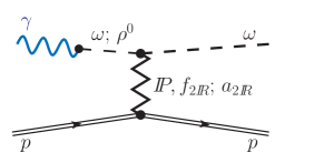
(a) (b)

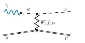
Figure 28: Photoproduction of an $\omega$ meson (a) via pomeron and subleading reggeon exchanges, and (b) as a result of $\phi$-$\omega$ mixing.

The diffractive amplitude for the $\gamma p\to\omega p$ reaction represented by the diagram (a) of Fig. 28 can be treated analogously as for the $\gamma p\to\rho^{0}p$ reaction, see Sec. II and Eqs. (2.9)–(2.11) of Lebiedowicz:2014bea , but with the replacements: $m_{\rho}\to m_{\omega}$, $\gamma_{\rho}\to\gamma_{\omega}$ (see (3.25) of Ewerz:2013kda ), $a_{\mathbb{P}\rho\rho}\to a_{\mathbb{P}\omega\omega}$, $b_{\mathbb{P}\rho\rho}\to b_{\mathbb{P}\omega\omega}$. $a_{f_{2\mathbb{R}}\rho\rho}\to a_{f_{2\mathbb{R}}\omega\omega}$, $b_{f_{2\mathbb{R}}\rho\rho}\to b_{f_{2\mathbb{R}}\omega\omega}$. In our case ($\gamma p\to\omega p$) the $a_{2\mathbb{R}}$-reggeon exchange cannot be neglected due to the large value of the $\gamma$-$\rho^{0}$ coupling constant; see (3.23)–(3.25) of Ewerz:2013kda . The propagators for $\mathbb{P}$, $f_{2\mathbb{R}}$, and $a_{2\mathbb{R}}$ will be taken as in (3.10), and (3.12), respectively, of Ewerz:2013kda . The couplings of $\mathbb{P}$, $f_{2\mathbb{R}}$, and $a_{2\mathbb{R}}$ to the proton will be taken according to (3.43), (3.49), and (3.51), respectively, of Ewerz:2013kda . Here, in analogy to $\gamma p\to\rho^{0}p$, we take $\Lambda_{0}^{2}=0.5$ GeV² in the form factor $F_{M}(t)$; see (2.11) of Lebiedowicz:2014bea and (3.34) of Ewerz:2013kda . In Fig. 28 the diagram (b) represents the $\phi$-$\omega$ mixing term to the process $\gamma p\to\omega p$. The procedure for determining the appropriate constants for this process is outlined below; see Eqs. (69), 70).

In order to estimate the relevant coupling parameters we shall assume that the $f_{2\mathbb{R}}\omega\omega$ couplings are similar to the $f_{2\mathbb{R}}\rho\rho$ ones. Then we take the default values for the $f_{2\mathbb{R}}\rho\rho$ and $a_{2\mathbb{R}}\rho\omega$ couplings estimated from VMD in Sec. 7.2, Eqs. (7.31), (7.32), (7.36), and (7.43), of Ewerz:2013kda :

$$a_{f_{2\mathbb{R}}\omega\omega}\approx a_{f_{2\mathbb{R}}\rho\rho}=2.92\;{\rm GeV^{-3}}\,,\quad b_{f_{2\mathbb{R}}\omega\omega}\approx b_{f_{2\mathbb{R}}\rho\rho}=5.02\;{\rm GeV^{-1}}\,,$$ (65)

$$a_{a_{2\mathbb{R}}\rho\omega}=2.56\;{\rm GeV^{-3}}\,,\quad b_{a_{2\mathbb{R}}\rho\omega}=4.68\;{\rm GeV^{-1}}\,.$$ (66)

In (66) we assume that both coupling constants are positive. To estimate the $\mathbb{P}\omega\omega$ coupling constants we use the relation:

$$2m_{\omega}^{2}\,a_{\mathbb{P}\omega\omega}+b_{\mathbb{P}\omega\omega}=4\beta_{\mathbb{P}\pi\pi}=7.04\;\mathrm{GeV}^{-1}\,,$$ (67)

in analogy to the corresponding one for the $\rho$ meson; see (7.27) of Ewerz:2013kda and (2.13) of Lebiedowicz:2014bea . Note that $a_{\mathbb{P}\omega\omega}$ must be positive in order to have a positive $\omega p$ total cross section for all $\omega$ polarisations. This follows from (7.21) of Ewerz:2013kda replacing there the $\rho$ by the $\omega$ meson.

In Fig. 29 we show the cross sections for the $\gamma p\to\omega p$ reaction together with the experimental data. From the comparison of our results to the experimental data, taking first only the diagrams of Fig. 28 (a) into account, we found that even a small (and positive) value of the $a_{\mathbb{P}\omega\omega}$ coupling leads to a reduction of the cross section. Therefore, for simplicity, we choose $a_{\mathbb{P}\omega\omega}=0$ in (67). The black solid line corresponds to the calculation including only the terms shown in the diagram (a) of Fig. 28. We used here the $\mathbb{P}\omega\omega$ coupling constants

$$a_{\mathbb{P}\omega\omega}=0\,,\quad b_{\mathbb{P}\omega\omega}=7.04\;{\rm GeV^{-1}}\,$$ (68)

and the parameters (65) and (66) for the reggeon exchanges. We recall that for all exchanges participating in the diagram (a) we take $\Lambda_{0}^{2}=0.5$ GeV² in the form factor $F_{M}(t)$; see (3.34) of Ewerz:2013kda .

Now we include the off-diagonal terms from the diagram of Fig. 28 (b). For estimating the coupling constants $a_{\mathbb{P}\widetilde{\phi}\omega}$ and $b_{\mathbb{P}\widetilde{\phi}\omega}$ we use (63) and the determination of $a_{\mathbb{P}\phi\phi}$ and $b_{\mathbb{P}\phi\phi}$ from the discussion of the $\gamma p\to\phi p$ reaction below. We get with the sets A and B, respectively, with $\Delta\theta_{V}=3.7^{\circ}$

$${\rm set\,A}:\;a_{\mathbb{P}\widetilde{\phi}\omega}=0.05\;{\rm GeV^{-3}}\,,\quad b_{\mathbb{P}\widetilde{\phi}\omega}=0.23\;{\rm GeV^{-1}}\,,\quad\Lambda_{0,\,\mathbb{P}\widetilde{\phi}\omega}^{2}=1.0\;{\rm GeV^{2}};$$ (69)

$${\rm set\,B}:\;a_{\mathbb{P}\widetilde{\phi}\omega}=0.07\;{\rm GeV^{-3}}\,,\quad b_{\mathbb{P}\widetilde{\phi}\omega}=0.19\;{\rm GeV^{-1}}\,,\quad\Lambda_{0,\,\mathbb{P}\widetilde{\phi}\omega}^{2}=4.0\;{\rm GeV^{2}}.$$ (70)

In a similar way the coupling parameters for $f_{2\mathbb{R}}$ exchange, $a_{f_{2\mathbb{R}}\widetilde{\phi}\omega}$ and $b_{f_{2\mathbb{R}}\widetilde{\phi}\omega}$, can be obtained. However, the $f_{2\mathbb{R}}\phi\phi$ couplings are expected to be very small. In practice, we do not consider an $f_{2\mathbb{R}}$-exchange contribution from the diagram of Fig. 30 (a) below. Here, we neglect also the $f_{2\mathbb{R}}$ exchange from the diagram of Fig. 28 (b).

The blue solid line in Fig. 29 corresponds to the calculation including in addition to the processes from diagram (a) of Fig. 28 the $\phi$-$\omega$ mixing effect for the $\mathbb{P}$ exchange [see diagram (b) of Fig. 28]. Our model calculation describes the total cross section fairly well  for energies ${\rm W}_{\gamma p}>10$ GeV. At low $\gamma p$ energies there are other processes contributing, such as the $\pi^{0}$-meson exchange, and the $\omega$ bremsstrahlung; see, e.g., Cisek:2011vt ; Yu:2017vvp for reviews and details concerning the exclusive $\omega$ production. We nicely describe also the differential cross section $d\sigma/d|t|$. We have checked that the complete results including the $\phi$-$\omega$ mixing effect with sets A (69) and B (70) differ only marginally.

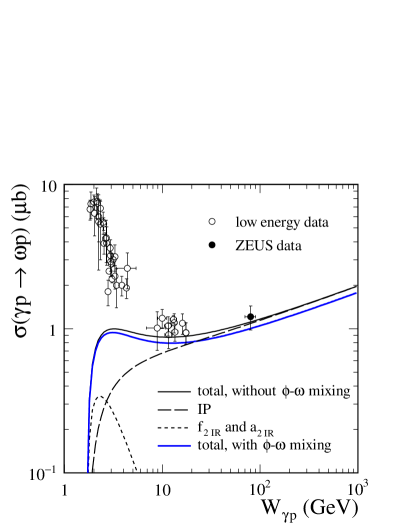
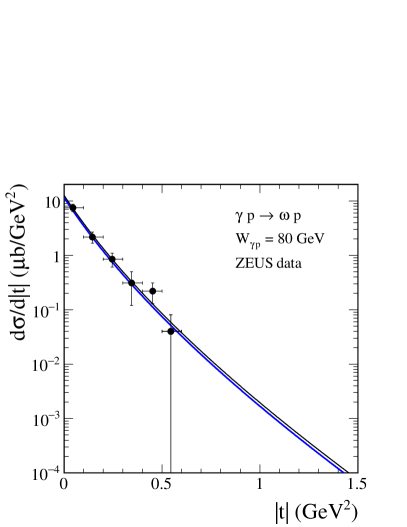
Figure 29: Left panel: The elastic $\omega$ photoproduction cross section as a function of the center-of-mass energy ${\rm W}_{\gamma p}$. Our results are compared with the ZEUS data Derrick:1996yt (at $\gamma p$ average c.m. energy $\langle{\rm W}_{\gamma p}\rangle=80~{}{\rm GeV}$) and with a compilation of low-energy experimental data (open circles; see the caption of Fig. 2 of Cisek:2011vt for more references). The black solid line corresponds to results with both the pomeron and reggeon ($f_{2\mathbb{R}}$, $a_{2\mathbb{R}}$) exchanges. The black long-dashed line corresponds to the pomeron exchange alone while the black short-dashed line corresponds to the reggeon term. In the calculation we used the parameters of the coupling constants given by (65), (66), and (68). The blue solid line corresponds to the complete result including the $\phi$-$\omega$ mixing effect (for the $\mathbb{P}$ exchange) with the parameter set A (69). Right panel: The differential cross section for the $\gamma p\to\omega p$ reaction at ${\rm W}_{\gamma p}=80~{}{\rm GeV}$. Our complete results, without (the black line) and with (the blue line) the mixing effect, are compared to the ZEUS data Derrick:1996yt .

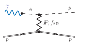
(a) (b)

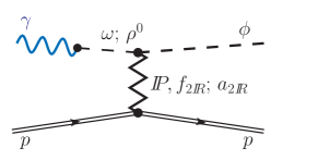
Figure 30: Photoproduction of a $\phi$ meson (a) via pomeron and subleading $f_{2\mathbb{R}}$ exchanges, and (b) as a result of $\omega$-$\phi$ mixing.

Next, we discuss the $\gamma p\to\phi p$ reaction. At high $\gamma p$ energies the pomeron exchange contribution, shown by the diagram (a) of Fig. 30, is the dominant one; see Sec. IV B of Lebiedowicz:2018eui . As was mentioned in Sec. I, in the low-energy region the corresponding production mechanism is not well established yet. There the nondiffractive processes of the pseudoscalar $\pi^{0}$- and $\eta$-meson exchange are known to contribute and are not negligible due to constructive $\eta$-$\pi^{0}$ interference; see, e.g., Titov:1999eu ; Titov:2003bk . In addition, many other processes, e.g., direct $\phi$ meson radiation via the $s$- and $u$-channel proton exchanges Titov:1999eu ; Kim:2019kef , $s\bar{s}$-cluster knockout Oh:2001bq , $t$-channel $\sigma$-, $f_{2}(1270)$- and $f_{1}(1285)$-exchanges Kong:2016scm were considered. In Kong:2016scm no vertex form factors were taken into account for the reggeized meson exchange contributions and instead of the $f_{2}(1270)$-exchange there one should consider $f_{2}^{\prime}$-exchange with appropriate parameters. However, a peak in the differential cross sections $(d\sigma/dt)_{t=t_{\rm min}}$ at forward angles around $E_{\gamma}\sim 2$ GeV (${\rm W}_{\gamma p}\sim 2.3$ GeV) observed by the LEPS Mibe:2005er ; Mizutani:2017wpg and CLAS Dey:2014tfa collaborations cannot be explained by the processes mentioned above. To explain the near-threshold bump structure the authors of Kiswandhi:2010ub ; Kiswandhi:2011cq ; Kim:2019kef propose to include exchanges with the excitation of nucleon resonances. In Ozaki:2009mj ; Ryu:2012tw another explanation, using the coupled-channel contributions with the $\Lambda(1520)$ resonance, was investigated. In Ryu:2012tw the hadronic box diagrams with the dominant $K\Lambda(1520)$ rescattering amplitude in the intermediate state were treated only approximately in a coupled-channel formalism neglecting the real part of the transition amplitudes.

Implementation of the box diagrams in our four-body calculation is rather cumbersome. On the other hand, we expect that they do not play a crucial role for the $pp\to pp\phi$ reaction at the high energies of interest to us here.

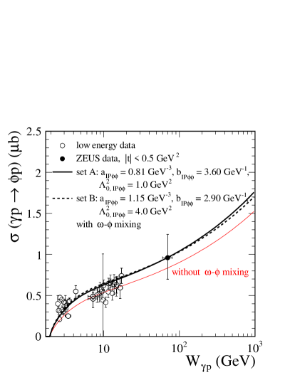
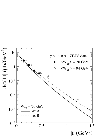
Figure 31: Left panel: The elastic $\phi$ photoproduction cross section as function of the center-of-mass energy ${\rm W}_{\gamma p}$. Our results are compared with the HERA data Derrick:1996af at ${\rm W}_{\gamma p}=70~{}{\rm GeV}$ and with a compilation of low-energy experimental data (see the caption of Fig. 6 of Lebiedowicz:2018eui for references). The upper lines represent results for two parameter sets, set A and set B, including the $\omega\to\phi$ transition terms with (74), (75), (76). Here we take in (19), in set A (72), $\Lambda_{0,\,\mathbb{P}\phi\phi}^{2}=1.0$ GeV² and, in set B (73), $\Lambda_{0,\,\mathbb{P}\phi\phi}^{2}=4.0$ GeV². The lower red line represents the result for the diagram (a) of Fig. 30 only with the parameter set (72). Right panel: The differential cross section $d\sigma/d|t|$ for the $\gamma p\to\phi p$ process. We show the ZEUS data at low $|t|$ (at ${\rm W}_{\gamma p}=70$ GeV and the squared photon virtuality $Q^{2}=0$ GeV², solid marks, Derrick:1996af ) and at higher $|t|$ (at ${\rm W}_{\gamma p}=94$ GeV and $Q^{2}<0.01$ GeV², open circles, Breitweg:1999jy ). Again, the results for the two parameter sets, set A (72) and set B (73), are presented.

In Fig. 31 we show the elastic $\phi$ photoproduction cross section as a function of the center-of-mass energy ${\rm W}_{\gamma p}$ (left panel) and the differential cross section $d\sigma/d|t|$ (right panel). To estimate the $\mathbb{P}\phi\phi$ coupling constants we use the relation [see Eq. (4.20) of Lebiedowicz:2018eui ]

$$2m_{\phi}^{2}\,a_{\mathbb{P}\phi\phi}+b_{\mathbb{P}\phi\phi}=4\,(2\beta_{\mathbb{P}KK}-\beta_{\mathbb{P}\pi\pi})=5.28\;\mathrm{GeV}^{-1}\,.$$ (71)

We show results for two parameter sets, set A and set B,

$${\rm set\,A}:\;a_{\mathbb{P}\phi\phi}=0.81\;{\rm GeV^{-3}}\,,\quad b_{\mathbb{P}\phi\phi}=3.60\;{\rm GeV^{-1}}\,,\quad\Lambda_{0,\,\mathbb{P}\phi\phi}^{2}=1.0\;{\rm GeV^{2}}\,,$$ (72)

$${\rm set\,B}:\;a_{\mathbb{P}\phi\phi}=1.15\;{\rm GeV^{-3}}\,,\quad b_{\mathbb{P}\phi\phi}=2.90\;{\rm GeV^{-1}}\,,\quad\Lambda_{0,\,\mathbb{P}\phi\phi}^{2}=4.0\;{\rm GeV^{2}}\,,$$ (73)

which were obtained based on the diagrams (a) and (b) of Fig. 30 including the diffractive $\omega$-$\phi$ transition terms with

$$a_{\mathbb{P}\widetilde{\omega}\phi}=0\,,\quad b_{\mathbb{P}\widetilde{\omega}\phi}=-0.46\;{\rm GeV^{-1}}$$ (74)

using (62) and (68). Similarly we obtain from (62) and (65), (66)

$$a_{f_{2\mathbb{R}}\widetilde{\omega}\phi}=-\tan(\Delta\theta_{V})\,a_{f_{2\mathbb{R}}\omega\omega}=-0.19\;{\rm GeV^{-3}}\,,$$

$$b_{f_{2\mathbb{R}}\widetilde{\omega}\phi}=-\tan(\Delta\theta_{V})\,b_{f_{2\mathbb{R}}\omega\omega}=-0.33\;{\rm GeV^{-1}}\,;$$ (75)

$$a_{a_{2\mathbb{R}}\widetilde{\rho}\phi}=-\tan(\Delta\theta_{V})\,a_{a_{2\mathbb{R}}\rho\omega}=-0.17\;{\rm GeV^{-3}}\,,$$

$$b_{a_{2\mathbb{R}}\widetilde{\rho}\phi}=-\tan(\Delta\theta_{V})\,b_{a_{2\mathbb{R}}\rho\omega}=-0.30\;{\rm GeV^{-1}}\,.$$ (76)

Note that the parameter set (72) for $\Lambda_{0,\,\mathbb{P}\phi\phi}^{2}=1.0\;{\rm GeV^{2}}$ is different than found by us in Sec. IV B of Lebiedowicz:2018eui (see Fig. 6 there)

$$a_{\mathbb{P}\phi\phi}=0.49\;{\rm GeV^{-3}}\,,\quad b_{\mathbb{P}\phi\phi}=4.27\;{\rm GeV^{-1}}\,,\quad\Lambda_{0,\,\mathbb{P}\phi\phi}^{2}=1.0\;{\rm GeV^{2}}\,,$$ (77)

where the $\omega$-$\phi$ mixing effect was not included. For comparison, the red lower line represents the result without the $\omega$-$\phi$ mixing, i.e., it contains only the terms represented by the diagram (a) of Fig. 30. We can see from Fig. 31 (right panel) that the parameter set B (73) for $\Lambda_{0,\,\mathbb{P}\phi\phi}^{2}=4.0\;{\rm GeV^{2}}$ with the relevant values of the coupling constants $a$ and $b$ describes more accurately the $t$ distribution.

In Fig. 32 we show the integrated cross section for the $\gamma p\to\phi p$ reaction at low ${\rm W}_{\gamma p}$ energies. We can see that the diffractive pomeron and reggeon exchanges, even including the pseudoscalar and scalar meson exchange contributions, are not sufficient to describe the low-energy data. Here we want to examine the uncertainties of the photoproduction contribution due to the meson exchanges in the $t$ channel. In the left panel, for the meson exchanges, we use the values of the coupling constants and the cutoff parameters from Titov:1999eu while in the right panel we choose $\Lambda_{\widetilde{M}NN}=\Lambda_{\phi\gamma\widetilde{M}}=1.2$ GeV in (86) and (87) below.

Our extrapolations of the cross section, using the theory applicable at high energies, represents the experimental data roughly on the average. But the scatter of the experimental data is quite considerable. Thus, it is impossible for us to draw any further conclusions concerning these low-energy results at the moment.

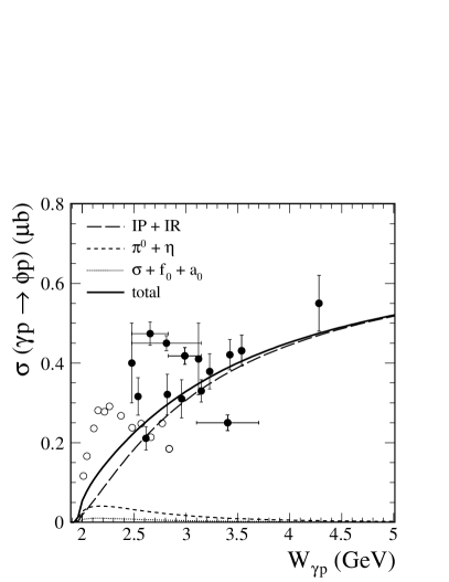
Figure 32: The elastic $\phi$ photoproduction cross section as a function of ${\rm W}_{\gamma p}$ integrated over $t_{\rm min}<|t|<1$ GeV². The theoretical results are compared with a compilation of low-energy experimental data from Ballam:1972eq ; Fries:1978di ; Barber:1981fj , and Laget:2000gj . The open data points are taken from Kong:2016scm (data was obtained there by integrating over the differential cross sections given in Dey:2014tfa ). The solid lines correspond to a coherent sum of pomeron, $f_{2\mathbb{R}}$ reggeon, pseudoscalar, and scalar exchanges. For the diffractive component ($\mathbb{P}+\mathbb{R}$) we take the set A of parameters from Fig. 31. The results for the pseudoscalar and scalar exchanges shown in the left panel were obtained with the parameters from Titov:1999eu ; see Appendix C, Sec. 1. In the right panel, for comparison, we show results obtained for different values of the cutoff parameters in the pseudoscalar term. Here we take $\Lambda_{\widetilde{M}NN}=\Lambda_{\phi\gamma\widetilde{M}}=1.2$ GeV in (86) and (87).

Appendix C Subleading contributions to $\phi$ CEP

In this section we discuss the following subleading processes contributing to $pp\to pp\phi$. The fusion processes $\gamma$-$\pi^{0}$, $\gamma$-$\eta$, $\gamma$-$\eta^{\prime}$, and $\gamma$-$f_{0}$, $\gamma$-$a_{0}$, and fusion processes involving vector mesons $\phi$-$\mathbb{P}$, $\omega$-$\mathbb{P}$, $\omega$-$f_{2\mathbb{R}}$, $\rho$-$\pi^{0}$, $\omega$-$\eta$, and $\omega$-$\eta^{\prime}$. We can have also $\omega$-$f_{0}$ and $\omega$-$f_{2}^{\prime}$ contributions. But these contributions are expected to be very small since the $\phi$ is nearly a pure $s\bar{s}$ state, the $\omega$ nearly a pure $u\bar{u}+d\bar{d}$ state. In the following we shall, therefore, neglect such contributions.

Below we present formulas for $\phi$ production with subsequent decay $\phi\to K^{+}K^{-}$. The formulas for $\phi$ production are obtained from those by the replacement (25).

The discussions of the subleading processes for $\phi$ CEP are very important for the comparison of our theory with the WA102 experimental results. See in particular Figs. 5 and 6 of Sec. IV.1. At LHC energies the subleading processes should be negligible for mid-rapidity $\phi$ production. In Secs. 1 and 2 of this Appendix we discuss $\gamma$-pseudoscalar- and $\gamma$-scalar-fusion contributions to $\phi$ CEP. The couplings which we find there can also be used to calculate subleading contributions to photoproduction of the $\phi$ meson. The corresponding results are shown together with the leading contributions in Fig. 32 of Appendix B.

C.1 $\gamma$-pseudoscalar-meson contributions

First we consider processes with pseudoscalar meson $\widetilde{M}=\pi^{0},\eta,\eta^{\prime}$ exchanges. The generic diagrams for these contributions are shown in Fig. 33 (a), (b). We have for the total $\gamma$-pseudoscalar-meson-fusion contribution

$${}^{(3)}{\cal M}_{pp\to ppK^{+}K^{-}}^{(\phi\to K^{+}K^{-})}=\sum_{\widetilde{M}=\pi^{0},\,\eta,\,\eta^{\prime}}\left({\cal M}^{(\gamma\widetilde{M})}_{pp\to ppK^{+}K^{-}}+{\cal M}^{(\widetilde{M}\gamma)}_{pp\to ppK^{+}K^{-}}\right)\,.$$ (78)

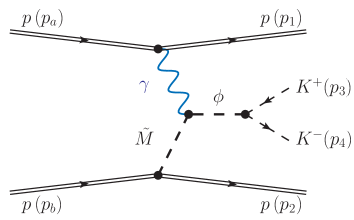
(a) (b)

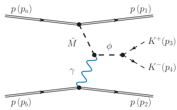
Figure 33: The Born-level diagrams for central-exclusive production of $\phi$ decaying to $K^{+}K^{-}$ in proton-proton collisions with pseudoscalar meson $\widetilde{M}$ exchange: (a) $\gamma$-$\widetilde{M}$ fusion; (b) $\widetilde{M}$-$\gamma$ fusion.

The $\gamma$-$\widetilde{M}$ amplitude can be written as

$${\cal M}^{(\gamma\widetilde{M})}_{pp\to ppK^{+}K^{-}} = (-i)\bar{u}(p_{1},\lambda_{1})i\Gamma^{(\gamma pp)}_{\mu}(p_{1},p_{a})u(p_{a},\lambda_{a})$$ (79)

$$\times i\Delta^{(\gamma)\,\mu\rho_{1}}(q_{1})\,i\Gamma^{(\phi\gamma\widetilde{M})}_{\rho_{2}\rho_{1}}(p_{34},q_{1})\,i\Delta^{(\phi)\,\rho_{2}\kappa}(p_{34})\,i\Gamma^{(\phi KK)}_{\kappa}(p_{3},p_{4})$$

$$\times i\Delta^{(\widetilde{M})}(t_{2})\,\bar{u}(p_{2},\lambda_{2})i\Gamma^{(\widetilde{M}pp)}(p_{2},p_{b})u(p_{b},\lambda_{b})\,.$$

For the $\widetilde{M}$-proton vertex we have (see (3.4) of Lebiedowicz:2016ryp )

$$i\Gamma^{(\widetilde{M}pp)}(p^{\prime},p)=-\gamma_{5}g_{\widetilde{M}pp}F^{(\widetilde{M}pp)}((p^{\prime}-p)^{2})\,.$$ (80)

We take $g_{\pi pp}=\sqrt{4\pi\times 14.0}$, $g_{\eta pp}=\sqrt{4\pi\times 0.99}$; see Eqs. (28) and (29) of Titov:1999eu .

An effective Lagrangian for the $\phi\gamma\widetilde{M}$ coupling is given in (22) of Titov:1999eu

$${\cal L}^{\prime}_{\phi\gamma\widetilde{M}}=\frac{e\,g_{\phi\gamma\widetilde{M}}}{m_{\phi}}\,\varepsilon^{\mu\nu\alpha\beta}\,(\partial_{\mu}\phi_{\nu})\,(\partial_{\alpha}A_{\beta})\,\widetilde{M}\,$$ (81)

with $A_{\beta}$ the photon field and $g_{\phi\gamma\widetilde{M}}$ a dimensionless coupling constant. From this we get the $\phi\gamma\widetilde{M}$ vertex, including a form factor, as follows
                

$$\begin{split}i\Gamma_{\mu\nu}^{(\phi\gamma\widetilde{M})}(p_{34},q_{1})=-ie\frac{g_{\phi\gamma\widetilde{M}}}{m_{\phi}}\,\varepsilon_{\mu\nu\rho\sigma}p_{34}^{\rho}q_{1}^{\sigma}\,\tilde{F}^{(\phi\gamma\widetilde{M})}(p_{34}^{2},q_{1}^{2},(p_{34}-q_{1})^{2})\,.\end{split}$$ (82)

We use a factorised ansatz for the $\phi\gamma\widetilde{M}$ form factor

$$\tilde{F}^{(\phi\gamma\widetilde{M})}(p_{34}^{2},q_{1}^{2},(p_{34}-q_{1})^{2})=\tilde{F}^{(\gamma)}(q_{1}^{2})\,\tilde{F}^{(\phi)}(p_{34}^{2})\,F^{(\phi\gamma\widetilde{M})}((p_{34}-q_{1})^{2})\,.$$ (83)

Based on considerations of the vector-meson-dominance model (VMD) we write the $\tilde{F}^{(\gamma)}$ form factor as

$$\tilde{F}^{(\gamma)}(q_{1}^{2})=\frac{m_{V}^{2}}{m_{V}^{2}-q_{1}^{2}}\,\tilde{F}^{(V)}(q_{1}^{2})$$ (84)

with $V=\rho^{0}$ for $\widetilde{M}=\pi^{0}$ and $V=\omega$ for $\widetilde{M}=\eta,\eta^{\prime}$. For the form factors $\tilde{F}^{(V)}$ we choose the form as for $\tilde{F}^{(\phi)}$ in (20) replacing $\phi$ by $V=\rho^{0},\omega$.

The effective coupling constant $g_{\phi\gamma\widetilde{M}}$ is related to the decay width of $\phi\to\gamma\widetilde{M}$, see (31) of Titov:1999eu ,

$$\Gamma(\phi\to\gamma\widetilde{M})=\frac{\alpha}{24}\frac{(m_{\phi}^{2}-m_{\widetilde{M}}^{2})^{3}}{m_{\phi}^{5}}|g_{\phi\gamma\widetilde{M}}|^{2}\,.$$ (85)

Using the most recent values from Tanabashi:2018oca , and taking the negative signs as in Titov:1999eu , we have found $g_{\phi\gamma\pi^{0}}=-0.137$, $g_{\phi\gamma\eta}=-0.705$, and $|g_{\phi\gamma\eta^{\prime}}|=0.726$. Note that $|g_{\phi\gamma\eta^{\prime}}|>|g_{\phi\gamma\eta}|$. But the contribution of $\eta^{\prime}$ exchange is suppressed relative to the $\eta$ exchange because of the heavier mass occurring in the propagator and of the smaller value of $g_{\eta^{\prime}pp}\simeq g_{\eta pp}/2$, where we follow Titov:1999eu . However, we note that there is no consensus on this latter relation in the literature. In Nakayama:1999jx $g_{\eta^{\prime}pp}\cong 6.1$ and $g_{\eta pp}=6.14$ are given.

We follow Titov:1999eu ; Titov:2003bk ; Ryu:2012tw and use monopole ansätze for the form factors $F^{(\widetilde{M}pp)}$ (80) and $F^{(\phi\gamma\widetilde{M})}$ (83)

$$F^{(\widetilde{M}pp)}(t)=\frac{\Lambda_{\widetilde{M}NN}^{2}-m_{\widetilde{M}}^{2}}{\Lambda_{\widetilde{M}NN}^{2}-t}\,,$$ (86)

$$F^{(\phi\gamma\widetilde{M})}(t)=\frac{\Lambda_{\phi\gamma\widetilde{M}}^{2}-m_{\widetilde{M}}^{2}}{\Lambda_{\phi\gamma\widetilde{M}}^{2}-t}\,.$$ (87)

The cutoff parameters $\Lambda_{\pi NN}=0.7$ GeV, $\Lambda_{\phi\gamma\pi}=0.77$ GeV, $\Lambda_{\eta NN}=1.0$ GeV, $\Lambda_{\phi\gamma\eta}=0.9$ GeV are taken from Titov:1999eu .

To examine uncertainties of the photoproduction contribution in the $pp\to pp\phi$ reaction we intend to show also the result with $\Lambda_{\widetilde{M}NN}=1.2$ GeV and $\Lambda_{\phi\gamma\widetilde{M}}=1.2$ GeV in (86) and (87), respectively, which are slightly different from the values given in Titov:1999eu . This choice of parameters was used in Kiswandhi:2011cq ; see Sec. II B there.

In Appendix B we discuss the $\gamma p\to\phi p$ reaction. There we compare our model calculations for different parameter sets with the experimental data.

Inserting (80)–(87) in (79) we can write the amplitude for the $\gamma\widetilde{M}$ exchange as follows

$${\cal M}^{(\gamma\widetilde{M})}_{pp\to ppK^{+}K^{-}} = i\,e^{2}\,\bar{u}(p_{1},\lambda_{1})\left[\gamma^{\alpha}F_{1}(t_{1})+\frac{i}{2m_{p}}\sigma^{\alpha\alpha^{\prime}}(p_{1}-p_{a})_{\alpha^{\prime}}F_{2}(t_{1})\right]u(p_{a},\lambda_{a})$$ (88)

$$\times\frac{1}{t_{1}}\,\frac{g_{\phi\gamma\widetilde{M}}}{m_{\phi}}\,\varepsilon_{\beta\alpha\rho\sigma}p_{34}^{\rho}q_{1}^{\sigma}\,\tilde{F}^{(\phi\gamma\widetilde{M})}(p_{34}^{2},q_{1}^{2},q_{2}^{2})$$

$$\times\Delta_{T}^{(\phi)}(p_{34}^{2})\,\frac{g_{\phi K^{+}K^{-}}}{2}\,(p_{3}-p_{4})^{\beta}\,F^{(\phi KK)}(p_{34}^{2})$$

$$\times\frac{1}{t_{2}-m_{\widetilde{M}}^{2}}\,g_{\widetilde{M}pp}\,F^{(\widetilde{M}pp)}(t_{2})\,\bar{u}(p_{2},\lambda_{2})\,\gamma_{5}\,u(p_{b},\lambda_{b})\,.$$

The amplitude ${\cal M}^{(\widetilde{M}\gamma)}_{pp\to ppK^{+}K^{-}}$ is obtained from (88) with the replacements (23).

C.2 $\gamma$-scalar-meson contributions

Next we turn to the amplitudes for $\phi$ production through the fusion of $\gamma$ with scalar mesons $S=f_{0}(500),f_{0}(980)$, and $a_{0}(980)$. Their contribution is

$${}^{(4)}{\cal M}_{pp\to ppK^{+}K^{-}}^{(\phi\to K^{+}K^{-})}=\sum_{S=f_{0}(500),\,f_{0}(980),\,a_{0}(980)}\left({\cal M}^{(\gamma S)}_{pp\to ppK^{+}K^{-}}+{\cal M}^{(S\gamma)}_{pp\to ppK^{+}K^{-}}\right)\,.$$ (89)

The generic diagrams for these contributions are as in Fig. 33 with $\widetilde{M}$ replaced by $S$. The same applies to the analytic expressions. We get ${\cal M}^{(\gamma S)}$ from ${\cal M}^{(\gamma\widetilde{M})}$ in (79) replacing $\Gamma_{\rho_{2}\rho_{1}}^{(\phi\gamma\widetilde{M})}$, $\Delta^{(\widetilde{M})}$, and $\Gamma^{(\widetilde{M}pp)}$ by $\Gamma_{\rho_{2}\rho_{1}}^{(\phi\gamma S)}$, $\Delta^{(S)}$, and $\Gamma^{(Spp)}$, respectively. We use the following expressions for the $S$-proton and for the $\phi\gamma S$ effective coupling Lagrangians, see (34) and (35), respectively, of Titov:1999eu ,

$${\cal L}^{\prime}_{Spp}=g_{Spp}\,\bar{p}\,p\,S\,,$$ (90)

$${\cal L}^{\prime}_{\phi\gamma S}=\frac{e\,g_{\phi\gamma S}}{m_{\phi}}\,(\partial^{\alpha}\phi^{\beta})\,(\partial_{\alpha}A_{\beta}-\partial_{\beta}A_{\alpha})\,S\,.$$ (91)

From these we get the vertices including form factors, as follows, where the momentum flow and the indices are chosen as for the $\widetilde{M}pp$ and $\phi\gamma\widetilde{M}$ vertices, respectively, see (80) and (82),

$$i\Gamma^{(Spp)}(p^{\prime},p)=ig_{Spp}F^{(Spp)}((p^{\prime}-p)^{2})\,,$$ (92)

$$i\Gamma_{\mu\nu}^{(\phi\gamma S)}(p_{34},q_{1})=-ie\frac{g_{\phi\gamma S}}{m_{\phi}}\,\left[q_{1\,\mu}p_{34\,\nu}-(p_{34}\cdot q_{1})g_{\mu\nu}\right]\,\tilde{F}^{(\phi\gamma S)}(p_{34}^{2},q_{1}^{2},(p_{34}-q_{1})^{2})\,.\qquad$$ (93)

For the contributions of scalar exchanges we take the parameters found in Appendix C of Titov:1999eu : $g_{\phi\gamma f_{0}(500)}=0.047$, $g_{f_{0}(500)pp}=\sqrt{4\pi\times 8.0}$, $g_{\phi\gamma f_{0}(980)}=-1.81$, $g_{f_{0}(980)pp}=0.56$, $g_{\phi\gamma a_{0}(980)}=-0.16$, $g_{a_{0}(980)pp}=21.7$. For $f_{0}(500)$ the monopole form of the form factors as in (86) and (87) with $\widetilde{M}$ replaced by $f_{0}(500)$ and $\Lambda_{f_{0}(500)NN}=\Lambda_{\phi\gamma f_{0}(500)}=2$ GeV is used. For the heavier mesons ($f_{0}(980)$ and $a_{0}(980)$) the following compact form is used Titov:1999eu :

$$F^{(Spp)}(t)F^{(\phi\gamma S)}(t)=\frac{\Lambda_{S}^{4}}{\Lambda_{S}^{4}+(t-m_{S}^{2})^{2}}\,,\quad\Lambda_{S}=0.6\;{\rm GeV}\,.$$ (94)

The final expression for the $\gamma S$-exchange amplitude in (89) reads

$${\cal M}^{(\gamma S)}_{pp\to ppK^{+}K^{-}} = \,e^{2}\,\bar{u}(p_{1},\lambda_{1})\left[\gamma^{\alpha}F_{1}(t_{1})+\frac{i}{2m_{p}}\sigma^{\alpha\alpha^{\prime}}(p_{1}-p_{a})_{\alpha^{\prime}}F_{2}(t_{1})\right]u(p_{a},\lambda_{a})$$ (95)

$$\times\frac{1}{t_{1}}\,\frac{g_{\phi\gamma S}}{m_{\phi}}\,\left[q_{1\,\beta}p_{34\,\alpha}-(p_{34}\cdot q_{1})g_{\beta\alpha}\right]\,\tilde{F}^{(\phi\gamma S)}(p_{34}^{2},q_{1}^{2},q_{2}^{2})$$

$$\times\Delta_{T}^{(\phi)}(p_{34}^{2})\,\frac{g_{\phi K^{+}K^{-}}}{2}\,(p_{3}-p_{4})^{\beta}\,F^{(\phi KK)}(p_{34}^{2})$$

$$\times\frac{1}{t_{2}-m_{S}^{2}}\,g_{Spp}\,F^{(Spp)}(t_{2})\,\bar{u}(p_{2},\lambda_{2})\,u(p_{b},\lambda_{b})\,.$$

For ${\cal M}^{(S\gamma)}_{pp\to ppK^{+}K^{-}}$ we have to make the replacements (23).

C.3 $\phi$-$\mathbb{P}$ and $\omega$-$\mathbb{P}$ contributions

Here we discuss two approaches, reggeized-vector-meson-exchange approach (I) and reggeon-exchange approach (II). For the second approach the corresponding diagrams are shown in Fig. 34.

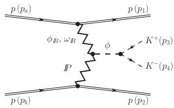
(a) (b)

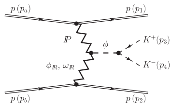
Figure 34: The Born-level diagrams for diffractive production of a $\phi$ meson with the subsequent decay $\phi\to K^{+}K^{-}$: (a) reggeon-pomeron fusion; (b) pomeron-reggeon fusion.

First we consider the contributions through the vector mesons $V=\phi$ and $\omega$:

$${}^{(5)}{\cal M}_{pp\to ppK^{+}K^{-}}^{(\phi\to K^{+}K^{-})}=\sum_{V=\phi,\,\omega}\left({\cal M}^{(V\mathbb{P})}_{pp\to ppK^{+}K^{-}}+{\cal M}^{(\mathbb{P}V)}_{pp\to ppK^{+}K^{-}}\right)\,.$$ (96)

The amplitude for the $V\mathbb{P}$-exchange can be written as

$${\cal M}^{(V\mathbb{P})}_{pp\to ppK^{+}K^{-}} = (-i)\bar{u}(p_{1},\lambda_{1})i\Gamma^{(Vpp)}_{\mu}(p_{1},p_{a})u(p_{a},\lambda_{a})$$ (97)

$$\times i\Delta^{(V)\,\mu\rho_{1}}(q_{1})\,i\Gamma^{(\mathbb{P}V\phi)}_{\rho_{2}\rho_{1}\alpha\beta}(p_{34},q_{1})\,i\Delta^{(\phi)\,\rho_{2}\kappa}(p_{34})\,i\Gamma^{(\phi KK)}_{\kappa}(p_{3},p_{4})$$

$$\times i\Delta^{(\mathbb{P})\,\alpha\beta,\delta\eta}(s_{2},t_{2})\,\bar{u}(p_{2},\lambda_{2})i\Gamma^{(\mathbb{P}pp)}_{\delta\eta}(p_{2},p_{b})u(p_{b},\lambda_{b})\,.$$

The $V$-proton vertex is

$$i\Gamma_{\mu}^{(Vpp)}(p^{\prime},p)=-ig_{Vpp}\,F^{(Vpp)}(t)\left[\gamma_{\mu}-i\frac{\kappa_{V}}{2m_{p}}\sigma_{\mu\nu}(p^{\prime}-p)^{\nu}\right],$$ (98)

with the tensor-to-vector coupling ratio, $\kappa_{V}=f_{Vpp}/g_{Vpp}$. Following Nakayama:1999jx we assume $\kappa_{\phi}=\kappa_{\omega}$ to be in the range $\simeq\pm 0.5$, $g_{\phi pp}=-0.6$ and $g_{\omega pp}=9.0$; see also Meissner:1997qt . Thus, the tensor term in (98) is small and in the calculation we take the vectorial term only with $g_{\phi pp}=-0.6$ and $g_{\omega pp}=8.65$. This latter value was determined in Sec. 6.3 of Ewerz:2013kda and, as discussed there, we assume $g_{\omega pp}=g_{\omega_{\mathbb{R}}pp}$.

We also make the assumption that the $t$-dependence of the $V$-proton coupling can be parametrised in a simple exponential form

$$F^{(Vpp)}(t)=\exp\left(\frac{t-m_{V}^{2}}{\Lambda_{VNN}^{2}}\right)\,,\quad\Lambda_{VNN}=1\;{\rm GeV}\,.$$ (99)

This form factor is normalized to unity when the vector meson $V$ is on its mass shell, i.e., when $t=m_{V}^{2}$.

The amplitude for the $V\mathbb{P}$-exchange can now be written as

$${\cal M}^{(V\mathbb{P})}_{pp\to ppK^{+}K^{-}}=-i\,g_{Vpp}\,F^{(Vpp)}(t_{1})\,\bar{u}(p_{1},\lambda_{1})\gamma^{\alpha}u(p_{a},\lambda_{a})$$

$$\qquad\times\Delta_{T}^{(V)}(t_{1})\,\Delta_{T}^{(\phi)}(p_{34}^{2})\,\frac{g_{\phi K^{+}K^{-}}}{2}\,(p_{3}-p_{4})^{\beta}\,F^{(\phi KK)}(p_{34}^{2})$$

$$\qquad\times\left[2a_{\mathbb{P}V\phi}\,\Gamma^{(0)}_{\beta\alpha\kappa\lambda}(p_{34},-q_{1})-b_{\mathbb{P}V\phi}\,\Gamma^{(2)}_{\beta\alpha\kappa\lambda}(p_{34},-q_{1})\right]F_{M}(q_{2}^{2})\,\tilde{F}^{(V)}(q_{1}^{2})\,\tilde{F}^{(\phi)}(p_{34}^{2})$$

$$\qquad\times\frac{1}{2s_{2}}\left(-is_{2}\alpha^{\prime}_{\mathbb{P}}\right)^{\alpha_{\mathbb{P}}(t_{2})-1}\,3\beta_{\mathbb{P}NN}\,F_{1}(t_{2})\,\bar{u}(p_{2},\lambda_{2})\left[\gamma^{\kappa}(p_{2}+p_{b})^{\lambda}\right]u(p_{b},\lambda_{b})\,.$$ (100)

For the $\mathbb{P}\phi\phi$ and $\mathbb{P}\omega\phi$ coupling vertices and constants see the discussion in the Appendices A and B.

For small values of $s_{1}=(p_{1}+p_{34})^{2}$ the standard form of the vector-meson propagator factor $\Delta_{T}^{(V)}(t_{1})$ in (100) should be adequate; see (16) for $V=\phi$. For higher values of $s_{1}$ we must take into account the reggeization. We do this, following (3.21), (3.24) of Lebiedowicz:2019jru , by making in the amplitude ${\cal M}^{(V\mathbb{P})}$ (100) the replacement

$$\Delta_{T}^{(V)}(t_{1})\to\Delta_{T}^{(V)}(t_{1})\left(\exp(i\phi(s_{1}))\,s_{1}\alpha^{\prime}_{V}\right)^{\alpha_{V}(t_{1})-1}\,,$$ (101)

$$\phi(s_{1})=\frac{\pi}{2}\exp\left(\frac{s_{\rm thr}-s_{1}}{s_{{\rm thr}}}\right)-\frac{\pi}{2}\,;$$ (102)

where $s_{\rm thr}$ is the lowest value of $s_{1}$ (4) possible here:

$$s_{\rm thr}=(m_{p}+2m_{K})^{2}\,.$$ (103)

Note, that in (101) we take $s_{1}\alpha^{\prime}_{V}$ instead of $s_{1}/s_{\rm thr}$ as in (3.21) of Lebiedowicz:2019jru . We assume for the Regge trajectories

$$\alpha_{V}(t)=\alpha_{V}(0)+\alpha^{\prime}_{V}\,t,\quad V=\phi,\,\omega,$$ (104)

$$\alpha_{\phi}(0)=0.1\,,\;\;\alpha^{\prime}_{\phi}=0.9\;{\rm GeV}^{-2}\,,$$ (105)

$$\alpha_{\omega}(0)=0.5\,,\;\;\alpha^{\prime}_{\omega}=0.9\;{\rm GeV}^{-2}\,;$$ (106)

see Eq. (5.3.1) of Collins:1977 .

Alternatively, we shall consider the exchange of the reggeons $\phi_{\mathbb{R}}$ and $\omega_{\mathbb{R}}$ instead of the mesons $\phi$ and $\omega$ as discussed above. We recall that $C=-1$ exchanges ($\omega_{\mathbb{R}}$, $\phi_{\mathbb{R}}$) are treated as effective vector exchanges in our model. In order to obtain the $\omega_{\mathbb{R}}\mathbb{P}$-exchange amplitude we make in (97) the following replacements:

$$\Gamma^{(Vpp)}_{\mu}(p_{1},p_{a})\to\Gamma^{(\omega_{\mathbb{R}}pp)}_{\mu}(p_{1},p_{a})\,,$$ (107)

$$\Delta^{(V)\,\mu\rho_{1}}(q_{1})\to\Delta^{(\omega_{\mathbb{R}})\,\mu\rho_{1}}(s_{1},t_{1})\,,$$ (108)

$$\Gamma^{(\mathbb{P}V\phi)}_{\rho_{2}\rho_{1}\alpha\beta}(p_{34},q_{1})\to\Gamma^{(\mathbb{P}\omega_{\mathbb{R}}\phi)}_{\rho_{2}\rho_{1}\alpha\beta}(p_{34},q_{1})\,.$$ (109)

We take the corresponding terms (107) and (108) from (3.59)–(3.60) and (3.14)–(3.15) of Ewerz:2013kda , respectively. In (109) we use the relations (62) and (74) and we take the factorised form for the $\mathbb{P}\omega_{\mathbb{R}}\phi$ form factor

$$F^{(\mathbb{P}\omega_{\mathbb{R}}\phi)}(q_{2}^{2},q_{1}^{2},p_{34}^{2})=F_{M}(q_{2}^{2})\,F_{M}(q_{1}^{2})\,F^{(\phi)}(p_{34}^{2})$$ (110)

with $F_{M}(q^{2})$ as in (19) but with $\Lambda_{0}^{2}=0.5$ GeV² and $F^{(\phi)}(p_{34}^{2})=F^{(\phi KK)}(p_{34}^{2})$; see (21). Then, the $\omega_{\mathbb{R}}\mathbb{P}$-exchange amplitude can be written as

$${\cal M}^{(\omega_{\mathbb{R}}\mathbb{P})}_{pp\to ppK^{+}K^{-}}=i\,g_{\omega_{\mathbb{R}}pp}\,F_{1}(t_{1})\,\bar{u}(p_{1},\lambda_{1})\gamma^{\alpha}u(p_{a},\lambda_{a})$$

$$\qquad\times\frac{1}{M_{-}^{2}}\left(-is_{1}\alpha^{\prime}_{\omega_{\mathbb{R}}}\right)^{\alpha_{\omega_{\mathbb{R}}}(t_{1})-1}\,\Delta_{T}^{(\phi)}(p_{34}^{2})\,\frac{g_{\phi K^{+}K^{-}}}{2}\,(p_{3}-p_{4})^{\beta}\,F^{(\phi KK)}(p_{34}^{2})$$

$$\qquad\times\left[2a_{\mathbb{P}\omega_{\mathbb{R}}\phi}\,\Gamma^{(0)}_{\beta\alpha\kappa\lambda}(p_{34},-q_{1})-b_{\mathbb{P}\omega_{\mathbb{R}}\phi}\,\Gamma^{(2)}_{\beta\alpha\kappa\lambda}(p_{34},-q_{1})\right]F^{(\mathbb{P}\omega_{\mathbb{R}}\phi)}(q_{2}^{2},q_{1}^{2},p_{34}^{2})$$

$$\qquad\times\frac{1}{2s_{2}}\left(-is_{2}\alpha^{\prime}_{\mathbb{P}}\right)^{\alpha_{\mathbb{P}}(t_{2})-1}\,3\beta_{\mathbb{P}NN}\,F_{1}(t_{2})\,\bar{u}(p_{2},\lambda_{2})\left[\gamma^{\kappa}(p_{2}+p_{b})^{\lambda}\right]u(p_{b},\lambda_{b})\,.\quad$$ (111)

We use for the parameter $M_{-}$ in the $\omega_{\mathbb{R}}$ propagator the value found in (3.14), (3.15) of Ewerz:2013kda

$$M_{-}=1.41\;\mathrm{GeV}\,.$$ (112)

In a similar way we obtain the $\phi_{\mathbb{R}}\mathbb{P}$-exchange amplitude. We assume that $g_{\phi_{\mathbb{R}}pp}=g_{\phi pp}$.

The ${\cal M}^{(\mathbb{P}V)}$ and ${\cal M}^{(\mathbb{P}V_{\mathbb{R}})}$ amplitudes are obtained from (100) and (111), respectively, with the replacements (23).

For the WA102 energy, $\sqrt{s}=29.1$ GeV, also the secondary $f_{2\mathbb{R}}$ exchange may play an important role. Setting $\sqrt{s_{1}}\approx\sqrt{s_{2}}$ [$\sqrt{s_{1}}$ and $\sqrt{s_{2}}$ are the energies of the subprocesses $p\,(p_{a})\,\mathbb{P}\,(q_{2})\to p\,(p_{1})\,\phi\,(p_{34})$ and $p\,(p_{b})\,\mathbb{P}\,(q_{1})\to p\,(p_{2})\,\phi\,(p_{34})$, respectively] and using the relation $s_{1}\,s_{2}\approx s\,m_{\phi}^{2}$ we obtain $\sqrt{s_{1}}\approx\sqrt{s_{2}}\approx 5.4$ GeV. Therefore, in interpreting the WA102 data it is necessary to take possible contributions from $\omega$-$f_{2\mathbb{R}}$ and $\omega_{\mathbb{R}}$-$f_{2\mathbb{R}}$ exchanges into account, in addition to the $\omega$-$\mathbb{P}$ and $\omega_{\mathbb{R}}$-$\mathbb{P}$ exchanges.

In a way similar to (97)–(111) we can write the amplitudes for the $\omega$-$f_{2\mathbb{R}}$ and $\omega_{\mathbb{R}}$-$f_{2\mathbb{R}}$ exchanges, since both, $\mathbb{P}$ and $f_{2\mathbb{R}}$ exchange, are treated as tensor exchanges in our model. The effective $f_{2\mathbb{R}}$-proton vertex function and the $f_{2\mathbb{R}}$ propagator are given in Ewerz:2013kda by Eqs. (3.49) and (3.12), respectively. As an example, the $\omega_{\mathbb{R}}f_{2\mathbb{R}}$-exchange amplitude can be written as in (111) with the following replacements:

$$\alpha_{\mathbb{P}}(t)\to\alpha_{\mathbb{R}_{+}}(t)\,,$$ (113)

$$3\beta_{\mathbb{P}NN}\to\frac{g_{f_{2\mathbb{R}}pp}}{M_{0}}\,,$$ (114)

$$a_{\mathbb{P}\omega_{\mathbb{R}}\phi}\to a_{f_{2\mathbb{R}}\omega_{\mathbb{R}}\phi}\,,\quad b_{\mathbb{P}\omega_{\mathbb{R}}\phi}\to b_{f_{2\mathbb{R}}\omega_{\mathbb{R}}\phi}\,,$$ (115)

$$F^{(\mathbb{P}\omega_{\mathbb{R}}\phi)}\to F^{(f_{2\mathbb{R}}\omega_{\mathbb{R}}\phi)}\,.$$ (116)

We take $\alpha_{\mathbb{R}_{+}}(t)=\alpha_{\mathbb{R}_{+}}(0)+\alpha^{\prime}_{\mathbb{R}_{+}}\,t$, $\alpha_{\mathbb{R}_{+}}(0)=0.5475$, $\alpha^{\prime}_{\mathbb{R}_{+}}=0.9$ GeV^-2 from (3.13) of Ewerz:2013kda and $g_{f_{2\mathbb{R}}pp}=11.04$, $M_{0}=1$ GeV from (3.50) of Ewerz:2013kda . For the $f_{2\mathbb{R}}\omega_{\mathbb{R}}\phi$ coupling parameters we assume that $a_{f_{2\mathbb{R}}\omega_{\mathbb{R}}\phi}=a_{f_{2\mathbb{R}}\widetilde{\omega}\phi}$, $b_{f_{2\mathbb{R}}\omega_{\mathbb{R}}\phi}=b_{f_{2\mathbb{R}}\widetilde{\omega}\phi}$ and use the relations (75). We assume that $F^{(f_{2\mathbb{R}}\omega_{\mathbb{R}}\phi)}=F^{(\mathbb{P}\omega_{\mathbb{R}}\phi)}$ (110) and take $\Lambda_{0}^{2}=0.5$ GeV².

In addition, we could have also the $\rho$-$a_{2\mathbb{R}}$ and $\rho_{\mathbb{R}}$-$a_{2\mathbb{R}}$ exchanges, but the couplings of $\rho_{\mathbb{R}}$ and $a_{2\mathbb{R}}$ to the protons are much smaller than those of $\omega_{\mathbb{R}}$ and $f_{2\mathbb{R}}$; see (3.62), (3.52), (3.60), and (3.50) of Ewerz:2013kda . Therefore, we neglect the $\rho$-$a_{2\mathbb{R}}$ and $\rho_{\mathbb{R}}$-$a_{2\mathbb{R}}$ terms in our considerations.

C.4 $\rho$-$\pi^{0}$ contribution

Finally, we consider the contribution from $\rho\pi^{0}$, respectively $\rho_{\mathbb{R}}\pi^{0}$, fusion.

$${}^{(6)}{\cal M}_{pp\to ppK^{+}K^{-}}^{(\phi\to K^{+}K^{-})}={\cal M}^{(\rho\pi^{0})}_{pp\to ppK^{+}K^{-}}+{\cal M}^{(\pi^{0}\rho)}_{pp\to ppK^{+}K^{-}}\,.$$ (117)

For the $\rho$-$\pi^{0}$ amplitude we have

$${\cal M}^{(\rho\pi^{0})}_{pp\to ppK^{+}K^{-}} = (-i)\bar{u}(p_{1},\lambda_{1})i\Gamma^{(\rho pp)}_{\mu}(p_{1},p_{a})u(p_{a},\lambda_{a})$$ (118)

$$\times i\Delta^{(\rho)\,\mu\rho_{1}}(q_{1})\,i\Gamma^{(\phi\rho\pi^{0})}_{\rho_{2}\rho_{1}}(p_{34},q_{1})\,i\Delta^{(\phi)\,\rho_{2}\kappa}(p_{34})\,i\Gamma^{(\phi KK)}_{\kappa}(p_{3},p_{4})$$

$$\times i\Delta^{(\pi^{0})}(t_{2})\,\bar{u}(p_{2},\lambda_{2})i\Gamma^{(\pi^{0}pp)}(p_{2},p_{b})u(p_{b},\lambda_{b})\,.$$

The $\rho$-proton vertex is given by (98) and (99) with $V=\rho$. The $\phi\rho\pi^{0}$ vertex is as the $\phi\gamma\widetilde{M}$ vertex in (82) with the replacements

$$\gamma\to\rho\,,\quad\widetilde{M}\to\pi^{0}\,,\quad eg_{\phi\gamma\widetilde{M}}\to g_{\phi\rho\pi^{0}}\,.$$ (119)

The proton-$\pi^{0}$ vertex is given in (80).

Then the $\rho$-$\pi^{0}$ amplitude can be written as

$${\cal M}^{(\rho\pi^{0})}_{pp\to ppK^{+}K^{-}} = i\,g_{\rho pp}\,F^{(\rho pp)}(t_{1})\,\bar{u}(p_{1},\lambda_{1})\left[\gamma^{\alpha}-i\frac{\kappa_{\rho}}{2m_{p}}\sigma^{\alpha\alpha^{\prime}}(p_{1}-p_{a})_{\alpha^{\prime}}\right]u(p_{a},\lambda_{a})$$ (120)

$$\times\Delta_{T}^{(\rho)}(t_{1})\,\Delta_{T}^{(\phi)}(p_{34}^{2})\,\frac{g_{\phi K^{+}K^{-}}}{2}\,(p_{3}-p_{4})^{\beta}\,F^{(\phi KK)}(p_{34}^{2})$$

$$\times\frac{g_{\phi\rho\pi}}{m_{\phi}}\,\varepsilon_{\beta\alpha\rho\sigma}p_{34}^{\rho}q_{1}^{\sigma}\,\tilde{F}^{(\rho)}(q_{1}^{2})\tilde{F}^{(\phi)}(p_{34}^{2})F^{(\phi\rho\pi^{0})}(q_{2}^{2})$$

$$\times\frac{1}{t_{2}-m_{\pi^{0}}^{2}}\,g_{\pi^{0}pp}\,F^{(\pi^{0}pp)}(t_{2})\,\bar{u}(p_{2},\lambda_{2})\,\gamma_{5}\,u(p_{b},\lambda_{b})\,.$$

We take $g_{\rho pp}=3.72$, $\kappa_{\rho}=6.1$, and $g_{\phi\rho\pi}=-1.258$ from Ryu:2012tw . Here we choose monopole form factors (86) and (87) with $\Lambda_{\pi^{0}pp}=1.2$ GeV and $\Lambda_{\phi\rho\pi^{0}}=1.2$ GeV, respectively. However, in Nakayama:1999jx smaller numerical values can be found, $g_{\rho pp}=2.63$–$3.36$ and $g_{\phi\rho\pi}=-0.65$, respectively. Therefore, our result should be considered rather as an upper limit for the $\rho$-$\pi^{0}$ contribution.

The reggeization of the $\rho$-meson propagator in the $t$-channel in ${\cal M}^{(\rho\pi^{0})}$ is taken into account here by the prescription (101) for $V=\rho$. We assume for the $\rho$ trajectory

$$\alpha_{\rho}(t)=\alpha_{\rho}(0)+\alpha^{\prime}_{\rho}\,t\,,$$ (121)

$$\alpha_{\rho}(0)=0.5\,,\;\;\alpha^{\prime}_{\rho}=0.9\;\mathrm{GeV}^{-2}\,.$$ (122)

The amplitude ${\cal M}^{(\pi^{0}\rho)}$ is obtained from ${\cal M}^{(\rho\pi^{0})}$ (118) by the replacements (23).

In principle we can also have $\omega$-$\eta$ and $\omega$-$\eta^{\prime}$ fusion contributions. $g_{\phi\omega\eta}$ and $g_{\phi\omega\eta^{\prime}}$ cannot be obtained from mesonic decays. Then one could rely only on models. Due to these model uncertainties of the coupling constants for the $\omega$-$\eta$ and $\omega$-$\eta^{\prime}$ fusion processes we neglect these contributions in our present study.

Appendix D The Collins-Soper frame

To make our present article self contained we give here the definition of the Collins-Soper (CS) frame used in our paper; see Lebiedowicz:2019por and for general remarks on various reference frames of this type Appendix A of Bolz:2014mya .

We go to the $K^{+}K^{-}$ or $\mu^{+}\mu^{-}$ rest frame for studying the reactions (1) or (35), respectively. Let $p_{a}$, $p_{b}$ be the three-momenta of the initial protons in this system. We define the unit vectors

$$\mbox{\boldmath$\hat{p}_{a}$}=\mbox{\boldmath$p_{a}$}/|\mbox{\boldmath$p_{a}$}|,\quad\mbox{\boldmath$\hat{p}_{b}$}=\mbox{\boldmath$p_{b}$}/|\mbox{\boldmath$p_{b}$}|\,.$$ (123)

The CS frame is then defined by the coordinate-axes unit vectors

$$\begin{split}&\mbox{\boldmath$e_{1}$}_{,\,\rm CS}=\frac{\mbox{\boldmath$\hat{p}_{a}$}+\mbox{\boldmath$\hat{p}_{b}$}}{|\mbox{\boldmath$\hat{p}_{a}$}+\mbox{\boldmath$\hat{p}_{b}$}|}\,,\\ &\mbox{\boldmath$e_{2}$}_{,\,\rm CS}=\frac{\mbox{\boldmath$\hat{p}_{a}$}\times\mbox{\boldmath$\hat{p}_{b}$}}{|\mbox{\boldmath$\hat{p}_{a}$}\times\mbox{\boldmath$\hat{p}_{b}$}|}\,,\\ &\mbox{\boldmath$e_{3}$}_{,\,\rm CS}=\frac{\mbox{\boldmath$\hat{p}_{a}$}-\mbox{\boldmath$\hat{p}_{b}$}}{|\mbox{\boldmath$\hat{p}_{a}$}-\mbox{\boldmath$\hat{p}_{b}$}|}\,.\end{split}$$ (124)

The angles $\theta_{K^{+},\,{\rm CS}}$ and $\phi_{K^{+},\,{\rm CS}}$, respectively $\theta_{\mu^{+},\,{\rm CS}}$ and $\phi_{\mu^{+},\,{\rm CS}}$, are the polar and azimuthal angles of the momentum vector $\hat{p}_{3}$ in this system. We have then, e.g.,

$$\cos\theta_{K^{+},\,{\rm CS}}=\mbox{\boldmath$\hat{p}_{3}$}\cdot\mbox{\boldmath$e_{3}$}_{,\,\rm CS}\,.$$ (125)

- (1) L. Łukaszuk and B. Nicolescu, A Possible interpretation of rising total cross-sections, Lett. Nuovo Cim. 8 (1973) 405.
- (2) D. Joynson, E. Leader, B. Nicolescu, and C. Lopez, Non-regge and hyper-regge effects in pion-nucleon charge exchange scattering at high energies, Nuovo Cim. A30 (1975) 345.
- (3) J. Kwieciński and M. Praszałowicz, Three gluon integral equation and odd singlet Regge singularities in QCD, Phys. Lett. B 94 (1980) 413.
- (4) J. Bartels, High-energy behavior in a non-abelian gauge theory (II). First corrections to beyond the leading approximation, Nucl. Phys. B 175 (1980) 365.
- (5) T. Jaroszewicz and J. Kwieciński, Odd gluonic regge singularities of perturbative QCD and their decoupling from deep inelastic neutrino scattering, Z. Phys. C12 (1982) 167.
- (6) R. Janik and J. Wosiek, Solution of the Odderon Problem, Phys. Rev. Lett. 82 (1999) 1092, arXiv:hep-th/9802100.
- (7) J. Bartels, L. N. Lipatov, and G. P. Vacca, A new odderon solution in perturbative QCD, Phys. Lett. B477 (2000) 178, arXiv:hep-ph/9912423 [hep-ph].
- (8) A. Breakstone et al., A Measurement of and Elastic Scattering in the Dip Region at GeV, Phys. Rev. Lett. 54 (1985) 2180.
- (9) G. Antchev et al., (TOTEM Collaboration), First determination of the parameter at TeV: probing the existence of a colourless -odd three-gluon compound state, Eur. Phys. J. C 79 no. 9, (2019) 785, arXiv:1812.04732 [hep-ex].
- (10) G. Antchev et al., (TOTEM Collaboration), Elastic differential cross-section at and implications on the existence of a colourless C-odd three-gluon compound state, Eur. Phys. J. C 80 no. 2, (2020) 91, arXiv:1812.08610 [hep-ex].
- (11) E. Martynov and B. Nicolescu, Did TOTEM experiment discover the Odderon?, Phys. Lett. B778 (2018) 414, arXiv:1711.03288 [hep-ph].
- (12) E. Martynov and B. Nicolescu, Evidence for maximality of strong interactions from LHC forward data, Phys. Lett. B786 (2018) 207, arXiv:1804.10139 [hep-ph].
- (13) V. A. Khoze, A. D. Martin, and M. G. Ryskin, Elastic proton-proton scattering at 13 TeV, Phys. Rev. D97 no. 3, (2018) 034019, arXiv:1712.00325 [hep-ph].
- (14) V. A. Khoze, A. D. Martin, and M. G. Ryskin, Black disk, maximal Odderon and unitarity, Phys. Lett. B780 (2018) 352, arXiv:1801.07065 [hep-ph].
- (15) V. A. Khoze, A. D. Martin, and M. G. Ryskin, Elastic and diffractive scattering at the LHC, Phys. Lett. B784 (2018) 192, arXiv:1806.05970 [hep-ph].
- (16) M. Broilo, E. Luna, and M. Menon, Forward Elastic Scattering and Pomeron Models, Phys. Rev. D98 no. 7, (2018) 074006, arXiv:1807.10337 [hep-ph].
- (17) A. Donnachie and P. V. Landshoff, Small elastic scattering and the parameter, Phys. Lett. B798 (2019) 135008, arXiv:1904.11218 [hep-ph].
- (18) T. Csörgo, R. Pasechnik, and A. Ster, Odderon and proton substructure from a model-independent Lévy imaging of elastic and collisions, Eur. Phys. J. C79 no. 1, (2019) 62, arXiv:1807.02897 [hep-ph].
- (19) I. Szanyi, N. Bence, and L. Jenkovszky, New physics from TOTEM’s recent measurements of elastic and total cross sections, J. Phys. G46 no. 5, (2019) 055002, arXiv:1808.03588 [hep-ph].
- (20) A. Schäfer, L. Mankiewicz, and O. Nachtmann, Double-diffractive and production as a probe for the odderon, Phys.Lett. B272 (1991) 419.
- (21) A. Bzdak, L. Motyka, L. Szymanowski, and J.-R. Cudell, Exclusive and hadroproduction and the QCD odderon, Phys.Rev. D75 (2007) 094023, arXiv:hep-ph/0702134 [hep-ph].
- (22) A. Cisek, W. Schäfer, and A. Szczurek, Exclusive photoproduction of meson in and reactions, Phys. Lett. B690 (2010) 168, arXiv:1004.0070 [hep-ph].
- (23) A. Cisek, W. Schäfer, and A. Szczurek, Exclusive photoproduction of charmonia in and reactions within -factorization approach, JHEP 1504 (2015) 159, arXiv:1405.2253 [hep-ph].
- (24) A. Cisek, P. Lebiedowicz, W. Schäfer, and A. Szczurek, Exclusive production of meson in proton-proton collisions at high energies, Phys.Rev. D83 (2011) 114004, arXiv:1101.4874 [hep-ph].
- (25) A. Schäfer, L. Mankiewicz, and O. Nachtmann, Diffractive , , and production in electron-proton collisions at HERA energies, in the proceedings of the workshop on Physics at HERA, Hamburg, Germany, October 29-30, 1991, p. 243. W. Buchmüller and G. Ingelman (eds.) DESY, 1992.
- (26) V. V. Barakhovsky, I. R. Zhitnitsky, and A. N. Shelkovenko, Odderon - a sharp signal at HERA, Phys. Lett. B267 (1991) 532.
- (27) W. Kilian and O. Nachtmann, Single pseudoscalar meson production in diffractive scattering, Eur. Phys. J. C5 (1998) 317, arXiv:hep-ph/9712371 [hep-ph].
- (28) E. R. Berger, A. Donnachie, H. G. Dosch, W. Kilian, O. Nachtmann, and M. Rüeter, Odderon and photon exchange in electroproduction of pseudoscalar mesons, Eur.Phys.J. C9 (1999) 491, arXiv:hep-ph/9901376 [hep-ph].
- (29) E. R. Berger, A. Donnachie, H. G. Dosch, and O. Nachtmann, Observing the odderon: Tensor meson photoproduction, Eur. Phys. J. C14 (2000) 673, arXiv:hep-ph/0001270 [hep-ph].
- (30) A. Donnachie, H. G. Dosch, and O. Nachtmann, The Missing Odderon, Eur.Phys.J. C45 (2006) 771, arXiv:0508196 [hep-ph].
- (31) C. Ewerz and O. Nachtmann, Chiral symmetry and diffractive neutral pion photo- and electroproduction, Eur.Phys.J. C49 (2007) 685, arXiv:0608082 [hep-ph].
- (32) A. Dumitru and T. Stebel, Multiquark matrix elements in the proton and three gluon exchange for exclusive production in photon-proton diffractive scattering, Phys. Rev. D99 no. 9, (2019) 094038, arXiv:1903.07660 [hep-ph].
- (33) L. Motyka and J. Kwieciński, Possible probe of the QCD odderon singularity through the quasidiffractive production in collisions, Phys. Rev. D58 (1998) 117501, arXiv:hep-ph/9802278 [hep-ph].
- (34) S. Braunewell and C. Ewerz, Perturbative odderon in quasidiffractive photon-photon scattering, Phys. Rev. D70 (2004) 014021, arXiv:hep-ph/0403197 [hep-ph].
- (35) S. J. Brodsky, J. Rathsman, and C. Merino, Odderon-Pomeron interference, Phys. Lett. B461 (1999) 114, arXiv:hep-ph/9904280 [hep-ph].
- (36) P. Hägler, B. Pire, L. Szymanowski, and O. V. Teryaev, Hunting the QCD-odderon in hard diffractive electroproduction of two pions, Phys. Lett. B535 (2002) 117, arXiv:hep-ph/0202231 [hep-ph]. [Erratum: Phys. Lett.B540,324(2002)].
- (37) P. Hägler, B. Pire, L. Szymanowski, and O. V. Teryaev, Pomeron-Odderon interference effects in electroproduction of two pions, Eur. Phys. J. C26 (2002) 261, arXiv:hep-ph/0207224 [hep-ph].
- (38) I. F. Ginzburg, I. P. Ivanov, and N. N. Nikolaev, Possibility of the odderon discovery via observation of charge asymmetry in the diffractive production at HERA, Eur. Phys. J.direct 5 no. 1, (2003) 002, arXiv:hep-ph/0207345 [hep-ph].
- (39) A. Bolz, C. Ewerz, M. Maniatis, O. Nachtmann, M. Sauter, and A. Schöning, Photoproduction of pairs in a model with tensor-pomeron and vector-odderon exchange, JHEP 1501 (2015) 151, arXiv:1409.8483 [hep-ph].
- (40) B. Pire, F. Schwennsen, L. Szymanowski, and S. Wallon, Hard Pomeron-Odderon interference effects in the production of pairs in high energy collisions at the LHC, Phys. Rev. D78 (2008) 094009, arXiv:0810.3817 [hep-ph].
- (41) C. Ewerz, The Odderon in Quantum Chromodynamics, arXiv:hep-ph/0306137 [hep-ph].
- (42) C. Ewerz, The Odderon: Theoretical Status and Experimental Tests, in 11th International Conference on Elastic and Diffractive Scattering: Towards High Energy Frontiers: The 20th Anniversary of the Blois Workshops, 17th Rencontre de Blois (EDS 05) Chateau de Blois, Blois, France, May 15-20, 2005. 2005. arXiv:hep-ph/0511196 [hep-ph].
- (43) C. Ewerz, O. Nachtmann, and R. Schicker, Central exclusive production at the LHC: Remarks by the organisers on an EMMI workshop, arXiv:1908.11792 [hep-ph].
- (44) V. P. Goncalves, Searching for the Odderon in the diffractive photoproduction at collisions, Eur. Phys. J. C79 no. 5, (2019) 408, arXiv:1811.07622 [hep-ph].
- (45) L. Harland-Lang, V. Khoze, A. Martin, and M. Ryskin, Searching for the Odderon in Ultraperipheral Proton–Ion Collisions at the LHC, Phys. Rev. D 99 no. 3, (2019) 034011, arXiv:1811.12705 [hep-ph].
- (46) V. P. Goncalves and W. K. Sauter, production in photon-induced interactions at a fixed target experiment at LHC as a probe of the odderon, Phys. Rev. D91 no. 9, (2015) 094014, arXiv:1503.05112 [hep-ph].
- (47) C. Ewerz, M. Maniatis, and O. Nachtmann, A Model for Soft High-Energy Scattering: Tensor Pomeron and Vector Odderon, Annals Phys. 342 (2014) 31, arXiv:1309.3478 [hep-ph].
- (48) C. Ewerz, P. Lebiedowicz, O. Nachtmann, and A. Szczurek, Helicity in Proton-Proton Elastic Scattering and the Spin Structure of the Pomeron, Phys. Lett. B763 (2016) 382, arXiv:1606.08067 [hep-ph].
- (49) L. Adamczyk et al., (STAR Collaboration), Single spin asymmetry in polarized proton-proton elastic scattering at GeV, Phys. Lett. B719 (2013) 62, arXiv:1206.1928 [nucl-ex].
- (50) D. Britzger, C. Ewerz, S. Glazov, O. Nachtmann, and S. Schmitt, The Tensor Pomeron and Low- Deep Inelastic Scattering, Phys. Rev. D100 no. 11, (2019) 114007, arXiv:1901.08524 [hep-ph].
- (51) P. Lebiedowicz, O. Nachtmann, and A. Szczurek, Exclusive central diffractive production of scalar and pseudoscalar mesons; tensorial vs. vectorial pomeron, Annals Phys. 344 (2014) 301–339, arXiv:1309.3913 [hep-ph].
- (52) P. Lebiedowicz, O. Nachtmann, and A. Szczurek, and Drell-Söding contributions to central exclusive production of pairs in proton-proton collisions at high energies, Phys. Rev. D91 (2015) 074023, arXiv:1412.3677 [hep-ph].
- (53) P. Lebiedowicz, O. Nachtmann, and A. Szczurek, Central exclusive diffractive production of the continuum, scalar and tensor resonances in and scattering within the tensor Pomeron approach, Phys. Rev. D93 (2016) 054015, arXiv:1601.04537 [hep-ph].
- (54) P. Lebiedowicz, O. Nachtmann, and A. Szczurek, Exclusive diffractive production of via the intermediate and states in proton-proton collisions within tensor pomeron approach, Phys. Rev. D94 no. 3, (2016) 034017, arXiv:1606.05126 [hep-ph].
- (55) P. Lebiedowicz, O. Nachtmann, and A. Szczurek, Central production of in collisions with single proton diffractive dissociation at the LHC, Phys. Rev. D95 no. 3, (2017) 034036, arXiv:1612.06294 [hep-ph].
- (56) P. Lebiedowicz, O. Nachtmann, and A. Szczurek, Central exclusive diffractive production of pairs in proton-proton collisions at high energies, Phys. Rev. D97 no. 9, (2018) 094027, arXiv:1801.03902 [hep-ph].
- (57) P. Lebiedowicz, O. Nachtmann, and A. Szczurek, Towards a complete study of central exclusive production of pairs in proton-proton collisions within the tensor Pomeron approach, Phys. Rev. D98 (2018) 014001, arXiv:1804.04706 [hep-ph].
- (58) P. Lebiedowicz, O. Nachtmann, and A. Szczurek, Central exclusive diffractive production of via the intermediate state in proton-proton collisions, Phys. Rev. D99 no. 9, (2019) 094034, arXiv:1901.11490 [hep-ph].
- (59) P. Lebiedowicz, O. Nachtmann, and A. Szczurek, Extracting the Pomeron-Pomeron- coupling in the reaction through the angular distribution of the pions, Phys. Rev. D101 no. 3, (2020) 034008, arXiv:1901.07788 [hep-ph].
- (60) D. Barberis et al., (WA102 Collaboration), A study of the centrally produced system in interactions at 450 GeV/, Phys. Lett. B432 (1998) 436, arXiv:hep-ex/9805018 [hep-ex].
- (61) A. Kirk, Resonance production in central collisions at the CERN Omega spectrometer, Phys.Lett. B489 (2000) 29, arXiv:0008053 [hep-ph].
- (62) J. M. Laget, Photoproduction of vector mesons at large momentum transfer, Phys.Lett. B489 (2000) 313, arXiv:hep-ph/0003213 [hep-ph].
- (63) Y.-s. Oh and H. C. Bhang, Asymmetries in photoproduction and the Okubo-Zweig-Iizuka violation, Phys. Rev. C64 (2001) 055207, arXiv:nucl-th/0104068 [nucl-th].
- (64) A. I. Titov, T. S. H. Lee, H. Toki, and O. Streltsova, Structure of the photoproduction amplitude at a few GeV, Phys. Rev. C60 (1999) 035205.
- (65) A. I. Titov and T. S. H. Lee, Spin effects and baryon resonance dynamics in meson photoproduction at few GeV, Phys. Rev. C67 (2003) 065205, arXiv:nucl-th/0305002 [nucl-th].
- (66) S. Ozaki, A. Hosaka, H. Nagahiro, and O. Scholten, Coupled-channel analysis for photoproduction with , Phys. Rev. C80 (2009) 035201, arXiv:0905.3028 [hep-ph]. [Erratum: Phys. Rev.C81,059901(2010)].
- (67) A. Kiswandhi, J.-J. Xie, and S. N. Yang, Is the nonmonotonic behavior in the cross section of photoproduction near threshold a signature of a resonance?, Phys. Lett. B691 (2010) 214, arXiv:1005.2105 [hep-ph].
- (68) A. Kiswandhi and S. N. Yang, Analysis of the near-threshold peak structure in the differential cross section of -meson photoproduction: Indication of a missing resonance with non-negligible strangeness content, Phys. Rev. C86 (2012) 015203, arXiv:1112.6105 [nucl-th]. [Erratum: Phys. Rev.C86,019904(2012)].
- (69) H.-Y. Ryu, A. I. Titov, A. Hosaka, and H.-C. Kim, photoprodution with coupled-channel effects, PTEP 2014 (2014) 023D03, arXiv:1212.6075 [hep-ph].
- (70) K.-J. Kong, H. Kim, and B.-G. Yu, Role of exchange in the process and scaling with the axial vector meson from a Reggeized model, Phys. Rev. D95 no. 1, (2017) 014020, arXiv:1611.01345 [hep-ph].
- (71) S.-H. Kim and S.-i. Nam, Pomeron, nucleon-resonance, and -meson contributions in -meson photoproduction, Phys. Rev. C100 no. 6, (2019) 065208, arXiv:1904.05133 [hep-ph].
- (72) J. D. Bjorken and S. D. Drell, Relativistic Quantum Fields. McGraw-Hill, New York, 1965.
- (73) P. Lebiedowicz and A. Szczurek, Revised model of absorption corrections for the process, Phys. Rev. D92 (2015) 054001, arXiv:1504.07560 [hep-ph].
- (74) R. A. Kycia, J. Chwastowski, R. Staszewski, and J. Turnau, GenEx: A simple generator structure for exclusive processes in high energy collisions, Commun. Comput. Phys. 24 no. 3, (2018) 860, arXiv:1411.6035 [hep-ph].
- (75) R. A. Kycia, J. Turnau, J. J. Chwastowski, R. Staszewski, and M. Trzebiński, The adaptive Monte Carlo toolbox for phase space integration and generation, Commun. Comput. Phys. 25 no. 5, (2019) 1547, arXiv:1711.06087 [hep-ph].
- (76) R. Kycia, P. Lebiedowicz, A. Szczurek, and J. Turnau, Triple Regge exchange mechanisms of four-pion continuum production in the reaction, Phys. Rev. D95 no. 9, (2017) 094020, arXiv:1702.07572 [hep-ph].
- (77) A. Donnachie and P. V. Landshoff, Total cross sections, Phys.Lett. B296 (1992) 227, arXiv:hep-ph/9209205 [hep-ph].
- (78) A. Donnachie, H. G. Dosch, P. V. Landshoff, and O. Nachtmann, Pomeron physics and QCD, Camb.Monogr.Part.Phys.Nucl.Phys.Cosmol. 19 (2002) 1–347.
- (79) M. Derrick et al., (ZEUS Collaboration), Measurement of elastic photoproduction at HERA, Phys. Lett. B377 (1996) 259, arXiv:hep-ex/9601009 [hep-ex].
- (80) J. Breitweg et al., (ZEUS Collaboration), Measurement of diffractive photoproduction of vector mesons at large momentum transfer at HERA, Eur. Phys. J. C14 (2000) 213, arXiv:hep-ex/9910038 [hep-ex].
- (81) M. Tanabashi et al., (Particle Data Group), Review of Particle Physics, Phys. Rev. D98 no. 3, (2018) 030001.
- (82) F. E. Close and A. Kirk, Glueball - filter in central hadron production, Phys.Lett. B397 (1997) 333, arXiv:hep-ph/9701222 [hep-ph].
- (83) D. Barberis et al., (WA102 Collaboration), A kinematical selection of glueball candidates in central production, Phys.Lett. B397 (1997) 339.
- (84) R. Sikora. Poster Central Exclusive Production with forward proton measurement in ATLAS presented at XIV ICFA School on Instrumentation in Elementary Particle Physics, La Habana, Cuba, 2017, https://indico.cern.ch/event/630418/sessions/259147/attachments/1575142/2496474/Sikora.pdf; Also at WE-Heraeus Physics School: QCD - Old Challenges and New Opportunities, Bad Honnef, Germany, 2017.
- (85) R. A. Ryutin, Central exclusive diffractive production of two-pion continuum at hadron colliders, Eur. Phys. J. C79 no. 12, (2019) 981, arXiv:1910.06683 [hep-ph].
- (86) P. Lebiedowicz and A. Szczurek, Exclusive and semiexclusive production of pairs with isobars and other resonances in the final state and the size of absorption effects, Phys. Rev. D98 no. 5, (2018) 053007, arXiv:1807.06069 [hep-ph].
- (87) M. Aaboud et al., (ATLAS Collaboration), Measurement of the exclusive process in proton-proton collisions at TeV with the ATLAS detector, Phys. Lett. B777 (2018) 303, arXiv:1708.04053 [hep-ex].
- (88) V. Petrov and R. Ryutin, Patterns of the exclusive double diffraction, J.Phys.G 35 (2008) 065004, arXiv:0711.2370 [hep-ph].
- (89) M. Ryskin, A. Martin, and V. Khoze, Soft processes at the LHC, II: soft-hard factorization breaking and gap survival, Eur.Phys.J.C 60 (2009) 265, arXiv:0812.2413 [hep-ph].
- (90) L. A. Harland-Lang, V. A. Khoze, and M. G. Ryskin, Modelling exclusive meson pair production at hadron colliders, Eur.Phys.J. C74 (2014) 2848, arXiv:1312.4553 [hep-ph].
- (91) M. Mieskolainen, GRANIITTI: A Monte Carlo Event Generator for High Energy Diffraction, arXiv:1910.06300 [hep-ph].
- (92) H.-M. Choi and C.-R. Ji, Mixing angles and electromagnetic properties of ground state pseudoscalar and vector meson nonets in the light-cone quark model, Phys. Rev. D59 (1999) 074015, arXiv:hep-ph/9711450 [hep-ph].
- (93) A. Kucukarslan and U.-G. Meissner, - mixing in chiral perturbation theory, Mod. Phys. Lett. A21 (2006) 1423, arXiv:hep-ph/0603061 [hep-ph].
- (94) W. Qian and B.-Q. Ma, Vector meson - mixing and their form factors in light-cone quark model, Phys. Rev. D78 (2008) 074002, arXiv:0809.4411 [hep-ph].
- (95) B.-G. Yu, T. K. Choi, and K.-J. Kong, Features of photoproduction off nucleon target at forward angles: dominance of exchange with Regge cuts and scaling of differential cross-sections, J. Phys. G46 no. 7, (2019) 075005, arXiv:1710.04511 [hep-ph].
- (96) M. Derrick et al., (ZEUS Collaboration), Measurement of elastic photoproduction at HERA, Z.Phys. C73 (1996) 73, arXiv:9608010 [hep-ex].
- (97) T. Mibe et al., (LEPS Collaboration), Diffractive -meson photoproduction on proton near threshold, Phys. Rev. Lett. 95 (2005) 182001, arXiv:nucl-ex/0506015 [nucl-ex].
- (98) K. Mizutani et al., (LEPS Collaboration), photoproduction on the proton at = 1.5 - 2.9 GeV, Phys. Rev. C96 no. 6, (2017) 062201, arXiv:1710.00169 [nucl-ex].
- (99) B. Dey, C. A. Meyer, M. Bellis, and M. Williams, (CLAS Collaboration), Data analysis techniques, differential cross sections, and spin density matrix elements for the reaction , Phys. Rev. C89 no. 5, (2014) 055208, arXiv:1403.2110 [nucl-ex]. [Addendum: Phys. Rev.C90,no.1,019901(2014)].
- (100) J. Ballam et al., Vector-Meson Production by Polarized Photons at 2.8, 4.7, and 9.3 GeV, Phys. Rev. D7 (1973) 3150.
- (101) D. C. Fries, P. Heine, H. Hirschmann, A. Markou, E. Seitz, H. J. Behrend, W. P. Hesse, W. A. McNeely, Jr., and T. Miyachi, - wave interference in photoproduction near threshold, Nucl. Phys. B143 (1978) 408.
- (102) D. P. Barber et al., A study of elastic photoproduction of low mass pairs from hydrogen in the energy range 2.8-4.8 GeV, Z. Phys. C12 (1982) 1.
- (103) K. Nakayama, J. W. Durso, J. Haidenbauer, C. Hanhart, and J. Speth, meson production in proton proton collisions, Phys. Rev. C60 (1999) 055209, arXiv:nucl-th/9904040 [nucl-th].
- (104) U.-G. Meissner, V. Mull, J. Speth, and J. W. van Orden, Strange vector currents and the OZI rule, Phys. Lett. B408 (1997) 381, arXiv:hep-ph/9701296 [hep-ph].
- (105) P. D. B. Collins, An introduction to Regge theory and high energy physics. Cambridge University Press, 1977.