ParaOpt: a parareal algorithm for optimality systems
Abstract.
The time parallel solution of optimality systems arising in PDE constrained optimization could be achieved by simply applying any time parallel algorithm, such as Parareal, to solve the forward and backward evolution problems arising in the optimization loop. We propose here a different strategy by devising directly a new time parallel algorithm, which we call ParaOpt, for the coupled forward and backward nonlinear partial differential equations. ParaOpt is inspired by the Parareal algorithm for evolution equations, and thus is automatically a two-level method. We provide a detailed convergence analysis for the case of linear parabolic PDE constraints. We illustrate the performance of ParaOpt with numerical experiments both for linear and nonlinear optimality systems.
1. Introduction
Time parallel time integration has become an active research area over the last decade; there is even an annual workshop now dedicated to this topic called the PinT (Parallel in Time) workshop, which started with the first such dedicated workshop at the USI in Lugano in June 2011. The main reason for this interest is the advent of massively parallel computers [5] with so many computing cores that spatial parallelization of an evolution problem saturates long before all cores have been effectively used. There are four classes of such algorithms: methods based on multiple shooting leading to the parareal algorithm [45, 2, 30, 33, 20, 11, 18, 40], methods based on waveform relaxation [32, 8, 19, 21, 13, 14, 31, 39, 1, 15], methods based on multigrid [27, 34, 53, 28, 6, 17, 7, 41, 4], and direct time parallel methods [42, 49, 50, 35, 10]; for a review of the development of PinT methods, see [9],[46] and the references therein.
A natural area where this type of parallelization could be used effectively is in PDE constrained optimization on bounded time intervals, when the constraint is a time dependent PDE. In these problems, calculating the descent direction within the optimization loop requires solving both a forward and a backward evolution problem, so one could directly apply time parallelization techniques to each of these solves [23, 24, 25, 26]. Parareal can also be useful in one-shot methods where the preconditioning operator requires the solution of initial value problems, see e.g. [52]. Another method, which has been proposed in [36, 48] in the context of quantum control, consists of decomposing the time interval into sub-intervals and defining intermediate states at sub-interval boundaries; this allows one to construct a set of independent optimization problems associated with each sub-interval in time. Each iteration of the method then requires the solution of these independent sub-problems in parallel, followed by a cheap update of the intermediate states. In this paper, we propose yet another approach based on a fundamental understanding of the parareal algorithm invented in [33] as a specific approximation of a multiple shooting method [20]. We construct a new time-parallel method called ParaOpt for solving directly the coupled forward and backward evolution problems arising in the optimal control context. Our approach is related to the multiple shooting paradigm [43], where the time horizon is decomposed into non-overlapping sub-intervals, and we solve for the unknown interface state and adjoint variables using an inexact Newton method so that the trajectories are continuous across sub-intervals. Additionally, a parareal-like approximation is used to obtain a cheap approximate Jacobian for the Newton solve. There are two potential benefits to our approach: firstly, it is known that for some control problems, long time horizons lead to difficulties in convergence for the optimization loop. Therefore, a multiple shooting approach allows us to deal with local subproblems on shorter time horizons, where we obtain faster convergence. Such convergence enhancement has also been observed in [3, 37, 38], and also more recently in [48]. Secondly, if we use parareal to parallelize the forward and backward sweeps, then the speedup ratio will be bounded above by , where is the number of sub-intervals and is the number of parareal iterations required for convergence. For many problems, especially the non-diffusive ones like the Lotka-Volterra problem we consider in Section 4.2, this ratio does not go above 4–5; this limits the potential speedup that can be obtained from this classical approach. By decomposing the control problem directly and conserving the globally coupled structure of the problem, we obtain higher speedup ratios, closer to ones that are achievable for two-level methods for elliptic problems.
Our paper is organized as follows: in Section 2, we present our PDE constrained optimization model problem, and ParaOpt for its solution. In Section 3 we give a complete convergence analysis of ParaOpt for the case when the PDE constraint is linear and of parabolic type. We then illustrate the performance of ParaOpt by numerical experiments in Section 4, both for linear and nonlinear problems. We present our conclusions and an outlook on future work in Section 5.
2. ParaOpt: a two-grid method for optimal control
Consider the optimal control problem associated with the cost functional
where is a fixed regularization parameter, is a target state, and the evolution of the state function is described by the non-linear equation
| (1) |
with initial condition , where is the control, which is assumed to enter linearly in the forcing term. The first-order optimality condition then reads
| (2) |
with the final condition , see [16] for a detailed derivation.
We now introduce a parallelization algorithm for solving the coupled problem (1–2). The approach we propose follows the ideas of the parareal algorithm, combining a sequential coarse integration on and parallel fine integration on subintervals.
Consider a subdivision of and two sets of intermediate states and corresponding to approximations of the state and the adjoint state at times and respectively. We denote by and the nonlinear solution operators for the boundary value problem (2) on the subinterval with initial condition and final condition , defined so that propagates the state forward to and propagates the adjoint backward to :
| (3) |
Using these solution operators, we can write the boundary value problem as a system of subproblems, which have to satisfy the matching conditions
| (4) |
This nonlinear system of equations can be solved using Newton’s method. Collecting the unknowns in the vector , we obtain the nonlinear system
Using Newton’s method to solve this system gives the iteration
| (5) |
where the Jacobian matrix of is given by
| (6) |
Using the explicit expression for the Jacobian gives us the componentwise linear system we have to solve at each Newton iteration:
| (7) |
Note that this system is not triangular: the are coupled to the and vice versa, which is clearly visible in the Jacobian in (6). This is in contrast to the initial value problem case, where the application of multiple shooting leads to a block lower triangular system.
The parareal approximation idea is to replace the derivative term by a difference computed on a coarse grid in (7), i.e., to use the approximations
| (8) |
where and are propagators obtained from a coarse discretization of the subinterval problem (3), e.g., by using only one time step for the whole subinterval. This is certainly cheaper than evaluating the derivative on the fine grid; the remaining expensive fine grid operations and in (7) can now all be performed in parallel. However, since (7) does not have a block triangular structure, the resulting nonlinear system would need to be solved iteratively. Each of these outer iterations is now very expensive, since one must evaluate the propagators , etc., by solving a coupled nonlinear local control problem. This is in contrast to initial value problems, where the additional cost of solving nonlinear local problems is justified, because the block lower triangular structure allows one to solve the outer problem by forward substitution, without the need to iterate. In order to reduce the cost of computing outer residuals, our idea is not to use the parareal approximation (8), but to use the so-called “derivative parareal” variant, where we approximate the derivative by effectively computing it for a coarse problem, see [12],
| (9) |
The advantage of this approximation is that the computation of , , etc. only involves linear problems. Indeed, for a small perturbation in , the quantities and can be computed by discretizing and solving the coupled differential equations obtained by differentiating (2). If is the solution of (2) with and , then solving the linear derivative system
| (10) | |||||
on a coarse time grid leads to
where is the Hessian of multiplied by , and is thus linear in . Similarly, to compute and for a perturbation in , it suffices to solve the same ODE system as (10), except the end-point conditions must be replaced by , . Therefore, if GMRES is used to solve the Jacobian system (5), then each matrix-vector multiplication requires only the solution of coarse, linear subproblems in parallel, which is much cheaper than solving coupled nonlinear subproblems in the standard parareal approximation (8).
To summarize, our new ParaOpt method consists of solving for the system
| (11) |
for and , where
| (12) |
is an approximation of the true Jacobian in (6). If the system (11) is solved using a matrix-free method, the action of the sub-blocks , , etc. can be obtained by solving coarse linear subproblems of the type (10). Note that the calculation of times a vector (without preconditioning) is embarrassingly parallel, since it only requires the solution of local subproblems of the type (10), with no additional coupling to other sub-intervals. Global communication is only required in two places: within the Krylov method itself (e.g. when calculating inner products), and possibly within the preconditioner. The design of an effective preconditioner is an important and technical topic that will be the subject of a future paper. Of course, for problems with small state spaces (e.g. for ODE control problems), direct methods may also be used, once the coefficients of are calculated by solving (10) for suitable choices of and .
Regardless of how (11) is solved, since we use an approximation of the Jacobian, the resulting inexact Newton method will no longer converge quadratically, but only linearly; this is true even in the case where the differential equation is linear. In the next section, we will analyze in detail the convergence of the method for the case of a diffusive linear problem.
3. Implicit Euler for the diffusive linear case
We now consider the method in a linear and discrete setting. More precisely, we focus on a control problem
| (13) |
where is a real, symmetric matrix with negative eigenvalues. The matrix can for example be a finite difference discretization of a diffusion operator in space. We will consider a discretize-then-optimize strategy, so the analysis that follows is done in a discrete setting.
3.1. Discrete formulation
To fix ideas, we choose the implicit Euler111We use the term ‘implicit Euler’ instead of ‘Backward Euler’ because the method is applied forward and backward in time. method for the time discretization; other discretizations will be studied in a future paper. Let , and . Then the implicit Euler method gives222 If the ODE system contains mass matrices arising from a finite element discretization, e.g., then one can analyze ParaOpt by introducing the change of variables , , so as to obtain with . Since is symmetric positive definite whenever is, the analysis is identical to that for (14), even though one would never calculate and in actual computations.
| (14) |
or, equivalently,
We minimize the cost functional
For the sake of simplicity, we keep the notations , and for the discrete variables, that is , and . Introducing the Lagrangian (see [29, 16] and also [22, 51, 47] for details)
the optimality systems reads:
| (15) | |||||
| (16) | |||||
| (17) | |||||
| (18) | |||||
| (19) | |||||
where we used the fact that is symmetric. If is the eigenvalue decomposition of , then the transformation , , allows us to diagonalize the equations (15)–(19) and obtain a family of decoupled optimality systems of the form
| (20) | |||||
| (21) | |||||
| (22) | |||||
| (23) | |||||
| (24) | |||||
where the , and are now scalars, and is an eigenvalue of . This motivates us to study the scalar Dahlquist problem
where is a real, negative number. For the remainder of this section, we will study the ParaOpt algorithm applied to the scalar variant (20)–(24), particularly its convergence properties as a function of .
Let us now write the linear ParaOpt algorithm for (20)–(24) in matrix form. For the sake of simplicity, we assume that the subdivision is uniform, that is , where satisfies and , see Figure 1. We start by eliminating interior unknowns, i.e., ones that are not located at the time points . For , (21) and (24) together imply
| (25) |
On the other hand, (23) implies
| (26) |
Combining (25) and (26) then leads to
| (27) |
Setting and , and using the notation , (see Figure 1), we obtain from (26) and (27) the equations
where
| (28) | |||||
| (29) |
In matrix form, this can be written as
or, in a more compact form,
| (30) |
Note that this matrix has the same structure as the Jacobian matrix in (6), except that for the linear case. In order to solve (30) numerically, we consider a second time step such that . In other words, for each sub-interval of length , the derivatives of the propagators , , , are approximated using a coarser time discretization with time step . The optimality system for this coarser time discretization has the form
where has the same form as above, except that and are replaced by and , i.e., the values obtained from the formulas (28) and (29) when one replaces by . Then the ParaOpt algorithm (11–12) for the linear Dahlquist problem can be written as
or, equivalently
| (31) |
Note that using this iteration, only a coarse matrix needs to be inverted.
3.2. Eigenvalue problem
In order to study the convergence of the iteration (31), we study the eigenvalues of the matrix , which are given by the generalized eigenvalue problem
| (32) |
with being the eigenvector associated with the eigenvalue . Since has two zero rows, the eigenvalue must have multiplicity at least two. Now let be a non-zero eigenvalue. (If no such eigenvalue exists, then the preconditioning matrix is nilpotent and the iteration converges in a finite number of steps.) Writing (32) componentwise yields
| (33) | |||||
| (34) | |||||
| (35) | |||||
| (36) |
where we have introduced the simplified notation
| (37) |
The recurrences (34) and (35) are of the form
| (38) |
where
Solving the recurrence (38) in together with the initial condition (33) leads to
| (39) |
whereas the recurrence (38) in simply gives
| (40) |
Combining (39) and (40), we obtain
so that (36) gives rise to , with
| (41) |
Since we seek a non-trivial solution, we can assume . Therefore, the eigenvalues of consist of the number zero (with multiplicity two), together with the roots of , which are all non-zero. In the next subsection, we will give a precise characterization of the roots of , which depend on , as well as on via the parameters , , and .
3.3. Characterization of eigenvalues
In the next two results, we describe the location of the roots of from the last section, or equivalently, the non-zero eigenvalues of the iteration matrix . We first establish the sign of a few parameters in the case , which is true for diffusive problems.
Lemma 1.
Let . Then we have , , and .
Proof.
By the definitions (28) and (37), we see that
which is between and , since for . Moreover, is an increasing function of by direct calculation, so that
which shows that . Next, we have by definition
Since and , both the numerator and the denominator are negative, so . Finally, we have
since and , so the first quotient inside the parentheses is necessarily smaller than the second quotient. ∎
We are now ready to prove a first estimate for the eigenvalues of the matrix .
Theorem 1.
Let be the polynomial defined in (41). For , the roots of are contained in the set , where
| (42) |
where , and is a real negative number.
Proof.
Since zero is not a root of , we can divide by and see that has the same roots as the function
Recall the change of variables
substituting into and multiplying the result by shows that is equivalent to
with
| (43) |
We will now show that has at most one root inside the unit disc ; since the transformation from to maps circles to circles, this would be equivalent to proving that has at most one root outside the disc . We now use the argument principle from complex analysis, which states that the difference between the number of zeros and poles of inside a closed contour is equal to the winding number of the contour around the origin. Since is a polynomial and has no poles, this would allow us to count the number of zeros of inside the unit disc. Therefore, we consider the winding number of the contour with
around the point , which is a real negative number. If we can show that intersects the negative real axis at at most one point, then it follows that the winding number around any negative real number cannot be greater than 1.
We now concentrate on finding values of such that . Since , it suffices to consider the range , and the other half of the range will follow by conjugation. Since is a product, we deduce that
We consider the two terms on the right separately.
-
•
For the first term, we have for all
since is real and positive. For , we obviously have , whereas for , we have if , and otherwise.
-
•
For the second term, observe that for , we have
Therefore, the second term is piecewise linear with slope , with a jump of size whenever changes sign, i.e., at , . Put within the range , we can write
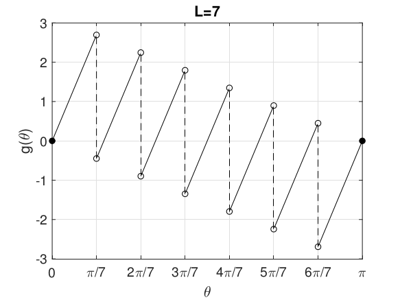
We also have by direct calculation. The function satisfies the property , see Figure 2.
From the above, we deduce that for all . Moreover,
Thus, the winding number around the point cannot exceed one, so at most one of the roots of can lie inside the unit disc. If there is indeed such a root , it must be real, since the conjugate of any root of is also a root. Moreover, it must satisfy , since for any . This implies
| (44) |
so the corresponding must also be negative. ∎
We have seen that the existence of depends on whether the constant is larger than 1. The following lemma shows that we indeed have .
Lemma 2.
Let . Then the constant , defined in (43), satisfies .
Proof.
We first transform the relation into a sequence of equivalent inequalities. Starting with the definition of , we have
where the last equivalence is obtained by multiplying both sides of the penultimate inequality by and then dividing it by . By the definition of and , the last inequality can be written as , where
with . Therefore, it suffices to show that is decreasing for . In other words, we need to show that
This is equivalent to showing
| (45) |
Using the fact that , we see that the left hand side is bounded above by
But for every and we have
| (46) |
see proof in the appendix. Therefore, (45) is satisfied by all and , so is in fact decreasing. It follows that , as required. ∎
Theorem 2.
Let be fixed, and let
| (47) |
Then the spectrum of has an eigenvalue outside the disc defined in (42) if and only if the number of subintervals satisfies , where is the regularization parameter.
Proof.
The isolated eigenvalue exists if and only if the winding number of about the origin is non-zero. Since only intersects the negative real axis at most once, we see that the winding number is non-zero when , i.e., when
Using the definition of , this leads to
hence the result. ∎
3.4. Spectral radius estimates
The next theorem now gives a more precise estimate on the isolated eigenvalue .
Theorem 3.
Suppose that the number of intervals satisfies , with defined in (47). Then the real negative eigenvalue outside the disc is bounded below by
Proof.
Suppose is a real root of inside the unit disc. We have seen at the end of the proof of Theorem 1 (page 3.3, immediately before Equation (44)) that ; moreover, since is assumed to be inside the unit circle, we must have . Therefore, satisfies . This implies
Therefore, satisfies
which means
Therefore,
where the last inequality is obtained by dropping the term containing inside the square root, which makes the square root larger since . ∎
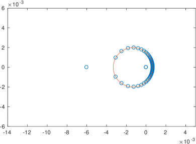
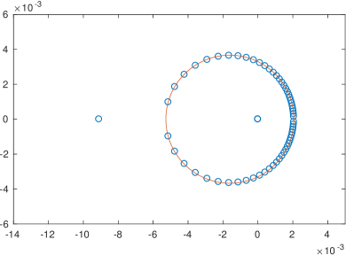
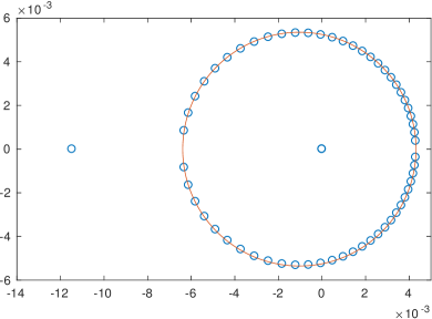
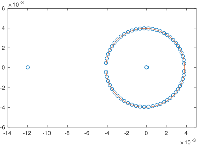
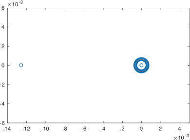
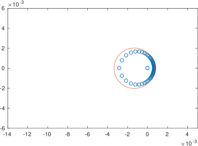
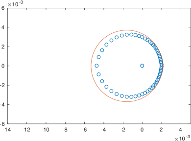
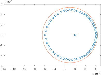
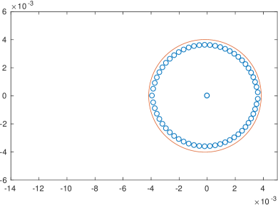
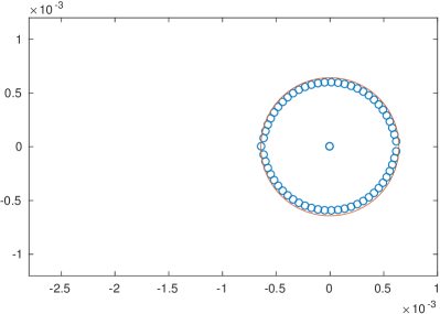
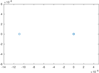
To illustrate the above theorems, we show in Figures 3 and 4 the spectrum of the iteration matrix for different values of and for and 1000. Here, the time interval is subdivided into subintervals, and each subinterval contains 50 coarse time steps and 5000 fine time steps. Table 1 shows the values of the relevant parameters. For , we see that there is always one isolated eigenvalue on the negative real axis, since in all cases, and its location is predicted rather accurately by the formula (48). The rest of the eigenvalues all lie within the disc defined in (42). For , the bounding disc is identical to the previous case; however, since we have for all cases except for , we observe no eigenvalue outside the disc, except for the very last case. In that very last case, we have , so (48) gives the lower bound , which again is quite accurate when compared with the bottom right panel of Figure 4.
| Radius of | bound () | |||||
| 0.6604 | 2.2462 | 0.8268 | 0.4280 | |||
| 0.4376 | 1.6037 | 0.6960 | 0.5300 | |||
| 0.1941 | 0.9466 | 0.4713 | 0.5539 | |||
| 0.0397 | 0.4831 | 0.1588 | 0.2930 | |||
| 0.0019 | 0.2344 | 0.0116 | 0.0417 | |||
| 0.0204 |

Corollary 1.
Let , , , , and be fixed. Then the spectral radius of the matrix satisfies
| (48) |
Note that the inequality (48) is valid for all , i.e., regardless of whether the isolated eigenvalue exists.
Proof.
When the number of sub-intervals satisfies , the spectral radius is determined by the isolated eigenvalue, which according to Theorem 3 is estimated by
Otherwise, when , all the eigenvalues lie within the bounding disc , so no eigenvalue can be farther away from the origin than
A straightforward calculation shows that
which is true by Lemma 2. Thus, the inequality (48) holds in both cases. ∎
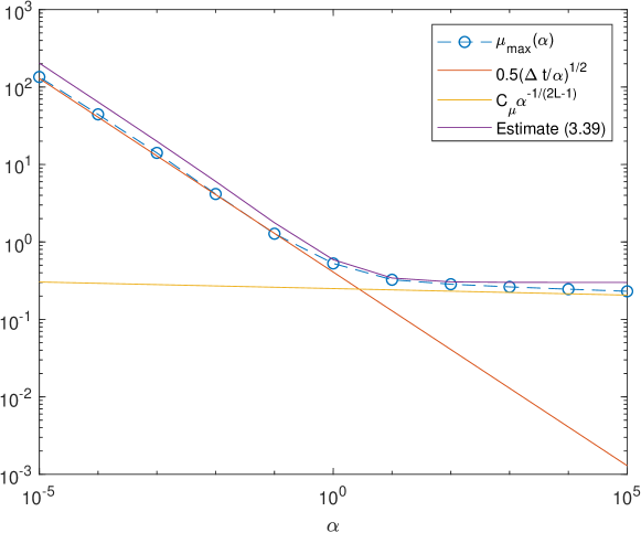
The above corollary is of interest when we apply our ParaOpt method to a large system of ODEs (arising from the spatial discretization of a PDE, for example), where the eigenvalues lie in the range , with when the spatial grid is refined. As we can see from Figure 5, the upper bound follows the actual spectral radius rather closely for most values of , and its maximum occurs roughly at the same value of as the one that maximizes the spectral radius. In the next two results, we will use the estimate (48) of the spectral radius of to derive a criterion for the convergence of the method.
Lemma 3.
Let , , , be fixed. Then for all , we have
| (49) |
Proof.
To bound , we start by bounding a scaled version of the quantity. We first use the definition of and (cf. (29)) to obtain
To estimate the terms and above, we define the mapping
so that , . Using the fact that for (see Lemma 5 in Appendix A), we see that
so is increasing. Therefore, we have
| (50) |
It then follows that
The last quotient is a function in only, whose maximum over all is approximately ; therefore, we have
For the second term, we use the mean value theorem and the fact that , to obtain
for some , with
Using the fact that for all , we deduce that
so that
Combining the estimates for and and multiplying by gives the first inequality in (49). For the second inequality, we use (50) to obtain
This is again a function in a single variable , whose maximum over all is approximately . ∎
Theorem 4.
Let , , and be fixed. Then for all , the spectral radius of satisfies
| (51) |
Thus, if , then the linear ParaOpt algorithm (31) converges.
Proof.
Starting with the spectral radius estimate (48), we divide the numerator and denominator by , then substitute its definition in (29) to obtain
Now, by Lemma 3, the first term is bounded above by
whose maximum occurs at with
Together with the estimate on in Lemma 3, this proves (51). Thus, a sufficient condition for the method (31) to converge can be obtained by solving the inequality
This is a quadratic equation in ; solving it leads to , as required. ∎
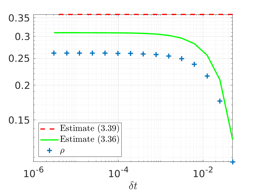
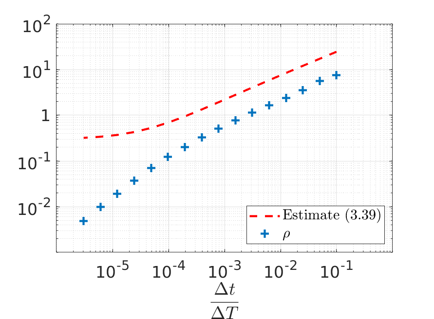
In Figure 6, we show the maximum spectral radius of over all negative for different values of for a model decomposition with
, 30 subintervals, one coarse time step per sub-interval, and a refinement ratio of
between the coarse and fine grid. We see in this case that the estimate (51) is indeed
quite accurate.
Remarks.
-
(1)
(Dependence on ) Theorem 4 states that in order to guarantee convergence, one should make sure that the coarse time step is sufficiently small relative to . In that case, the method converges.
-
(2)
(Weak scalability) Note that the estimate (51) depends on the coarse time step , but not explicitly on the number of sub-intervals . One may then consider weak scalability, i.e. cases where the problem size per processor is fixed333On the contrary, strong scalability deals with cases where the total problem size is fixed., under two different regimes: (i) keeping the sub-interval length and refinement ratios , fixed, such that adding subintervals increases the overall time horizon ; and (ii) keeping the time horizon fixed and refinement ratios , fixed, such that adding sub-intervals decreases their length . In the first case, remains fixed, so the bound (51) remains bounded as . In the second case, as , so in fact (51) decreases to as . Therefore, the method is weakly scalable under both regimes.
-
(3)
(Contraction rate for high and low frequencies) Let be fixed, and let be the spectral radius of as a function of given by (48). Then for , an asymptotic expansion shows that we have
In other words, the method reduces high and low frequency error modes very quickly, and the overall contraction rate is dominated by mid frequencies (where “mid” depends on , , etc). This is also visible in Figure 5, where attains its maximum at and decays quickly for both large and small .
Finally, we note that for the linear problem, it is possible to use Krylov acceleration to solve for the fixed point of (31), even when the spectral radius is greater than 1. However, the goal of this linear analysis is to use it as a tool for studying the asymptotic behaviour of the nonlinear method (11); since a contractive fixed point map must have a Jacobian with spectral radius less than 1 at the fixed point, Theorem 4 shows which conditions are sufficient to ensure asymptotic convergence of the nonlinear ParaOpt method.
4. Numerical results
In the previous section, we have presented numerical examples related to the efficiency of our bounds with respect to and . We now study in more detail the quality of our bounds with respect to the discretization parameters. We complete these experiments with a nonlinear example and a PDE example.
4.1. Linear scalar ODE: sensitivity with respect to the discretization parameters
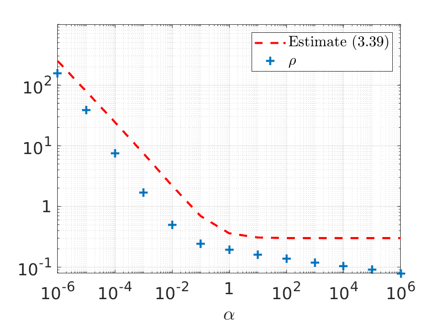
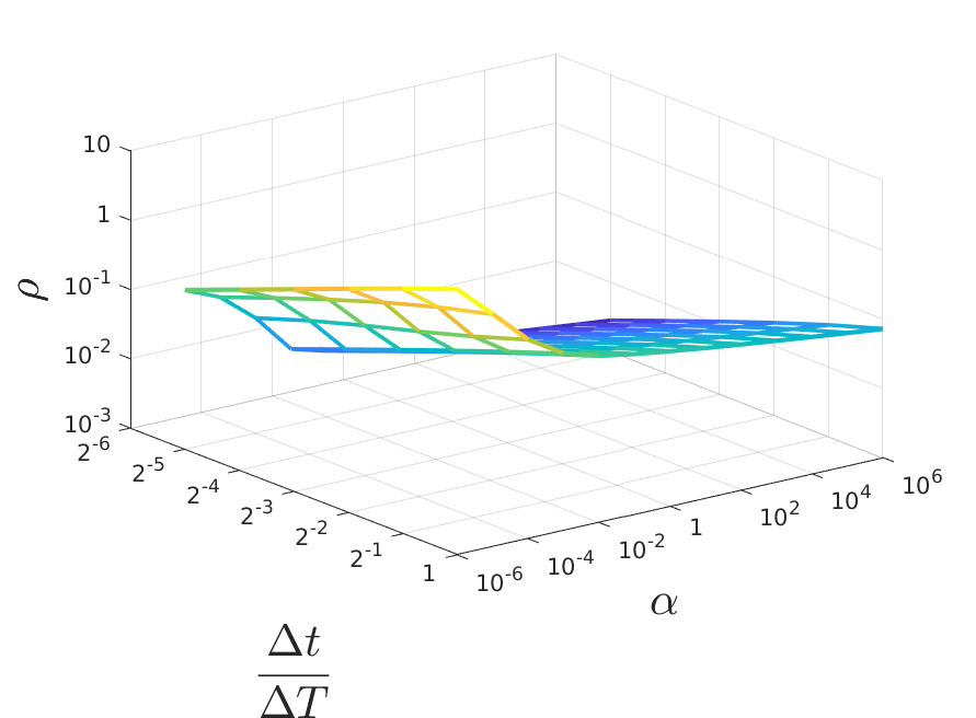
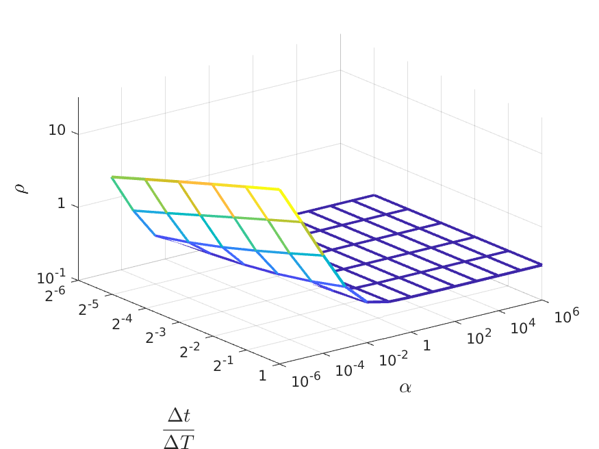
In this part, we consider the case where , and and investigate the dependence of the spectral radius of when , , vary.
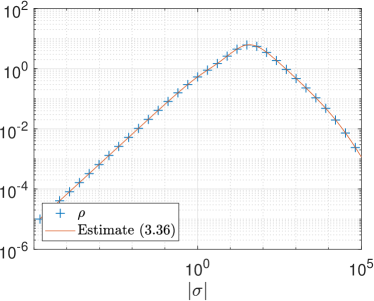
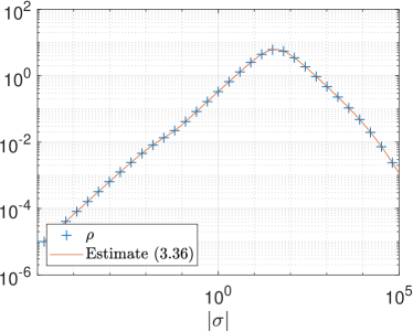
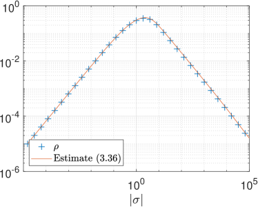
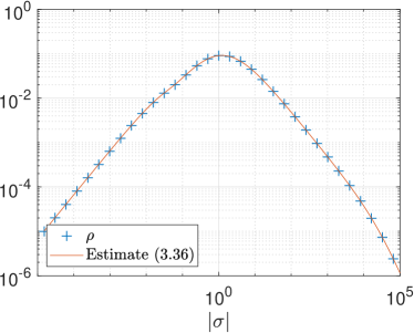
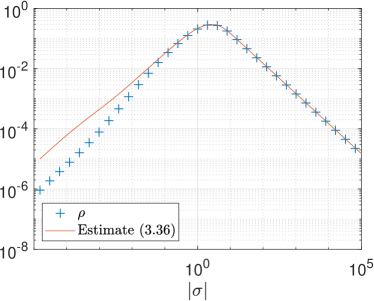
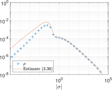
We start with variations in and , and a fixed number of sub-intervals . In this way, we compute the spectral radius of for three cases: first with a fixed and , ; then with a fixed and , ; and finally with a fixed ratio with , . The results are shown in Figure 7.
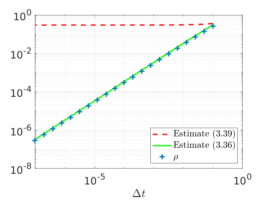
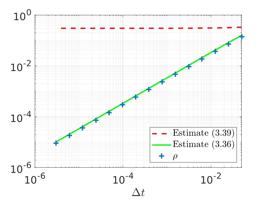
In all cases, we observe a very good agreement between the estimate obtained in (48) and the true spectral radius. Note that the largest possible for this problem is when equals the length of the sub-interval, i.e., when . For this , the estimates (3.36) and (3.39) are very close to each other, because (3.39) is obtained from (3.36) by making as large as possible, i.e., by letting .
We next study the scalability properties of ParaOpt. More precisely, we examine the behaviour of the spectral radius of the preconditioned matrix when the number of subintervals varies. In order to fit with the paradigm of numerical efficiency, we set which corresponds somehow to a coarsening limit. We consider two cases: the first case uses a fixed value of , namely , and the second case uses for the fixed value of . The results are shown in Figure 8.
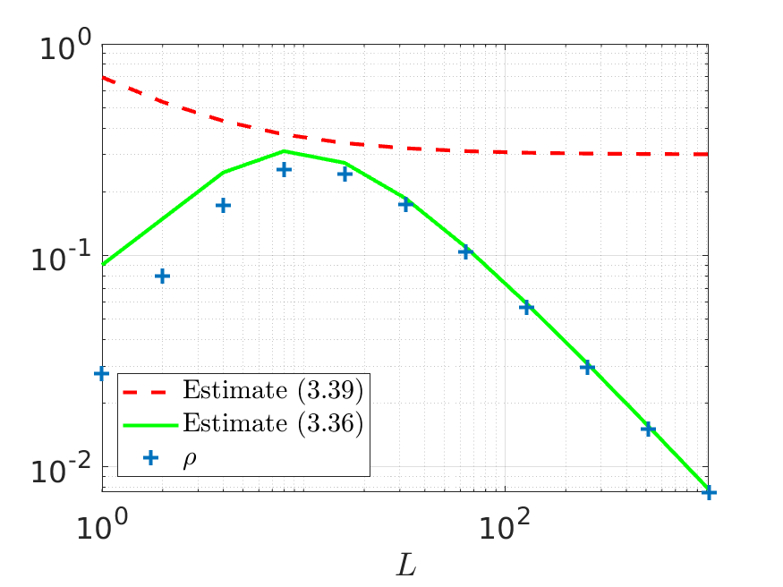
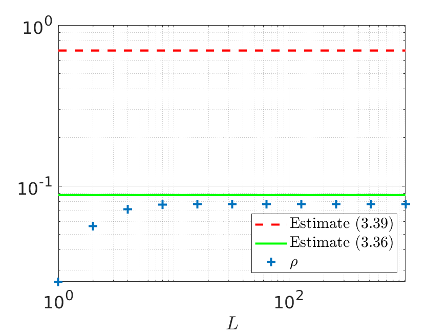
In both cases, we observe perfect scalability of ParaOpt, in the sense that the spectral radius is uniformly bounded with respect to the number of subintervals considered in the time parallelization.
4.2. A nonlinear example
We now consider a control problem associated with a nonlinear vectorial dynamics, namely the Lotka-Volterra system. The problem consists of minimizing the cost functional
with , subject to the Lotka-Volterra equations
| (52) | ||||
with , and initial conditions . In this nonlinear setting, the computation of each component of for given and requires a series of independent iterative inner loops. In our test, these computations are carried out using a Newton method. As in Section 3, the time discretization of (2) is performed with an implicit Euler scheme.
In a first test, we set and and fix the fine time discretization step to , with . In Figure 9, we show the rate of convergence of ParaOpt for and various values of the ratio . Here, the error is defined as the maximum difference between the interface state and adjoint values obtained from a converged fine-grid solution, and the interface values obtained at each inexact Newton iteration by ParaOpt.
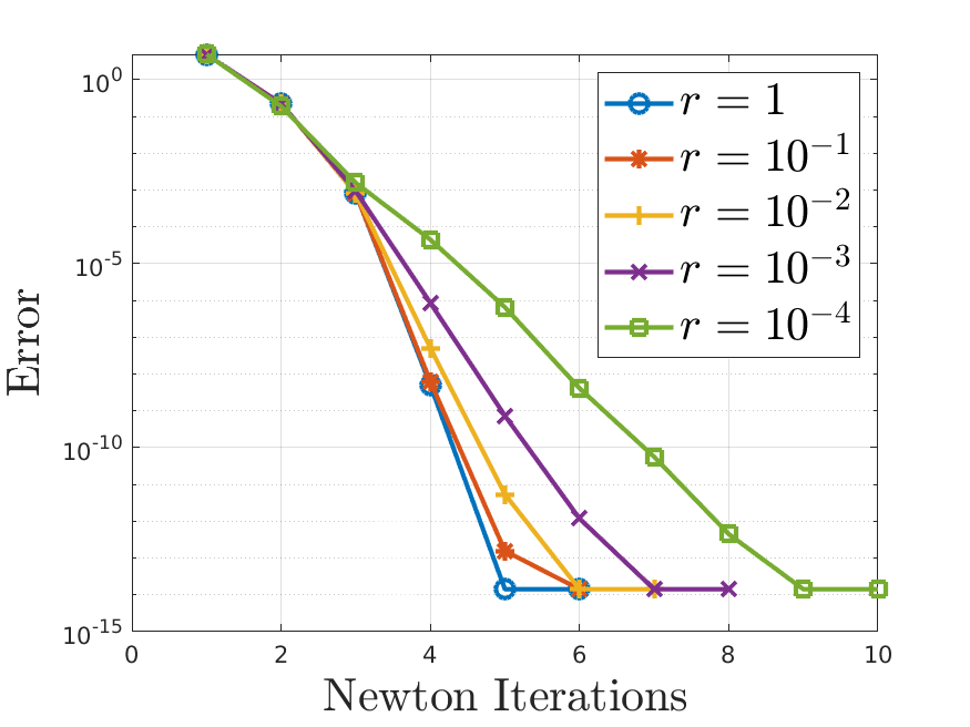
As can be expected when using a Newton method, we observe that quadratic convergence is obtained in the case . When becomes smaller, the preconditioning becomes a coarser approximation of the exact Jacobian, and thus convergence becomes a bit slower.
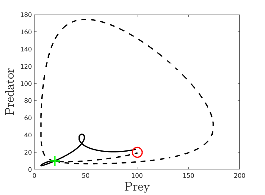
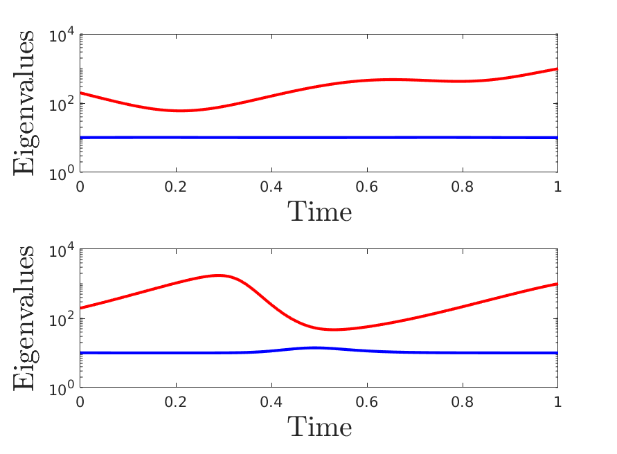
In our experiments, we observed that the initial guess plays a significant role in the convergence of the method. This follows from the fact that ParaOpt is an exact (if ) or approximate (otherwise) Newton method. The initial guess we consider is , , and . While for we observe convergence for all , if we increase to , we do not observe convergence any more for ; in fact, without decomposing the time domain, the sequential version of our solver with does not converge, even if we use the exact Jacobian without the coarse approximation. This shows that using a time-domain decomposition actually helps in solving the nonlinear problem, a phenomenon already observed for a different time-parallelization method in [48]. These convergence problems we observed are also related to the existence of multiple solutions. Indeed, if we coarsen the outer iteration by replacing the Newton iteration with a Gauss-Newton iteration, i.e., by removing the second order derivatives of and in Newton’s iterative formula, we obtain another solution, as illustrated in Figure 10 on the left for and . For both solutions, we observe that the eigenvalues associated with the linearized dynamics
in a neighborhood of the local minima remain strictly positive along the trajectories, in contrast to the situation analyzed in Section 3. Their values are presented in Figure 10 on the right.
We next test the numerical efficiency of our algorithm. The example we consider corresponds to the last curve of Figure 9, i.e. and , except that we use various values of using the corresponding number of processors. We execute our code in parallel on workers of a parallel pool, using Matlab’s Parallel Processing Toolbox on a 24-core machine that is part of the SciBlade cluster at Hong Kong Baptist University. The results are presented in Table 2, where we also indicate the total parallel computing time without communication, as well as the number of outer Newton iterations required for convergence to a tolerance of .
| Newton Its. | Parallel computing time | speedup | ||
|---|---|---|---|---|
| 1 | 14 | 777.53 | 777.42 | 1.00 |
| 3 | 10 | 172.13 | 167.36 | 4.52 |
| 6 | 9 | 82.10 | 79.67 | 9.47 |
| 12 | 9 | 43.31 | 42.49 | 17.95 |
| 24 | 9 | 25.75 | 24.74 | 30.20 |
We observe that our cluster enables us to get very good scalability, the total computing time is roughly divided by two when the number of processors is doubled. Though not reported in the table, we have observed that even in the case , i.e., without parallelization, ParaOpt outperforms the Newton method ( vs. in our test).
To see how this compares with speedup ratios that can be expected from more classical approaches, we run parareal on the initial value problem (52) with the same initial conditions and no control, i.e., . For and 24 sub-intervals and a tolerance of , parareal requires and 13 iterations to converge. (For a more generous tolerance of , parareal requires and 7 iterations.) Since the speedup obtained by parareal cannot exceed , the maximum speedup that can be obtained if parareal is used as a subroutine for forward and backward sweeps does not exceed 4 for our problem. Note that this result is specific to the non-diffusive character of the considered equation. This speedup would change if the constraint type changed to parabolic, see [44, chap. 5].
4.3. A PDE example
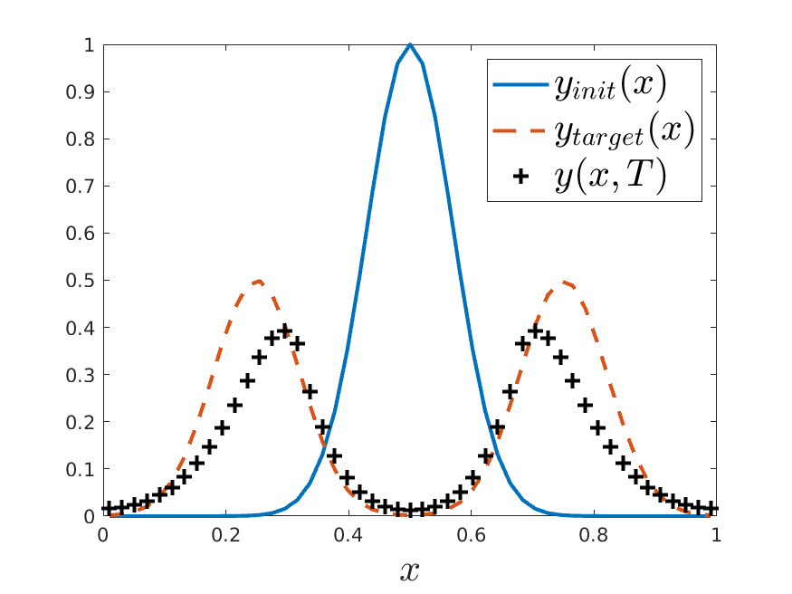
We finally consider a control problem involving the heat equation. More precisely, Eq. (1) is replaced by
where the unknown is defined on with periodic boundary conditions, and on with . Initial and target states are
The operator is the indicator function of a sub-interval of ; in our case, . We also set . The corresponding solution is shown in Figure 11.
We use a finite difference scheme with grid points for the spatial discretization. As in the previous subsection, an implicit Euler scheme is used for the time discretization, and we consider a parallelization involving subintervals, with and so that the rate of convergence of the method can be tested for various values of . For , the evolution of the error along the iterations is shown in Figure 12. Here, the error is defined as the maximum difference between the iterates and the reference discrete solution, evaluated at sub-interval interfaces.
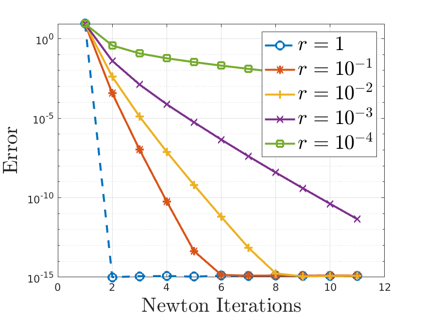
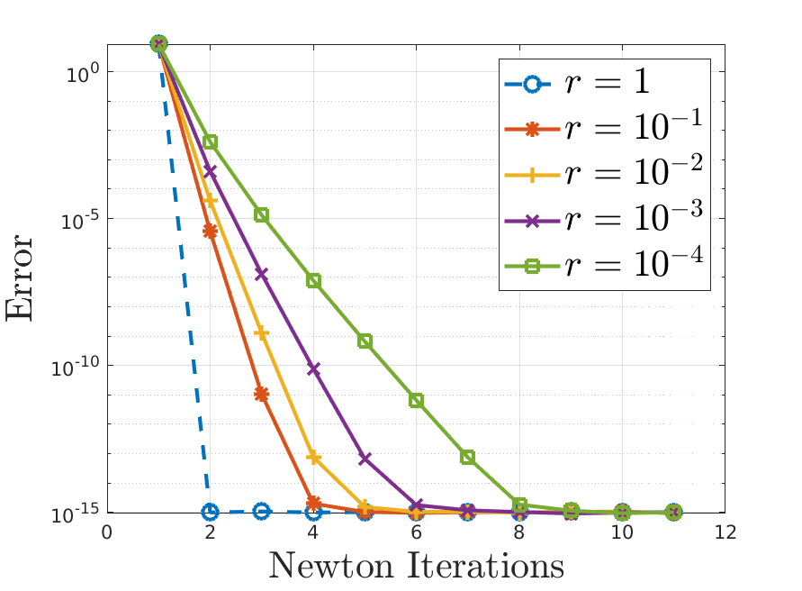
Observe also that the convergence curves corresponding to and on the left panel look nearly identical to the curves for and on the right panel. This is because they correspond to the same values of , namely and . This behavior is consistent with Theorem 4, where the convergence estimate depends only on , rather than on the ratio . Cases of divergence can also be observed, in particular for and small values of and , as shown in Figure 13.
Of course, one can envisage using different spatial discretizations for the coarse and fine propagators; this may provide additional speedup, provided suitable restriction and prologation operators are used to communicate between the two discretizations. This will be the subject of investigation in a future paper.
5. Conclusions
We introduced a new time-parallel algorithm we call ParaOpt for time-dependent optimal control problems. Instead of applying Parareal to solve separately the forward and backward equations as they appear in an optimization loop, we propose in ParaOpt to partition the coupled forward-backward problem directly in time, and to use a Parareal-like iteration to incorporate a coarse correction when solving this coupled problem. We analyzed the convergence properties of ParaOpt, and proved in the linear diffusive case that its convergence is independent of the number of sub-intervals in time, and thus scalable. We also tested ParaOpt on scalar linear optimal control problems, a nonlinear non-diffusive optimal control problem involving the Lotka-Volterra system, and also on a control problem governed by the heat equation. A small scale parallel implementation of the Lotka-Volterra case also showed scalability of ParaOpt for this nonlinear problem.
Our ongoing work consists of analyzing the algorithm for non-diffusive problems. Also, for problems with large state spaces, e.g., for discretized PDEs in three spatial dimensions, the approximate Jacobian in (12) may become too large to solve by direct methods. Thus, we are currently working on designing efficient preconditioners for solving such systems iteratively. Finally, we are currently studying ParaOpt by applying it to realistic problems from applications, in order to better understand its behaviour in such complex cases.
Acknowledgments
The authors acknowledge support from ANR Ciné-Para (ANR-15-CE23-0019), ANR/RGC ALLOWAPP (ANR-19-CE46-0013/A-HKBU203/19), the Swiss National Science Foundation grant no. 200020_178752, and the Hong Kong Research Grants Council (ECS 22300115 and GRF 12301817). We also thank the anonymous referees for their valuable suggestions, which greatly improved our paper.
Appendix A Proof of Inequality (46)
Our goal is to prove the following lemma, which is needed for the proof of Lemma 2.
Lemma 4.
For every and , we have
| (53) |
First, we need the following property of logarithmic functions.
Lemma 5.
For any , we have
Proof.
Let . Then
The conclusion now follows. ∎
Proof.
(Lemma 4) Let and denote the left and right hand sides of (53) respectively. We consider two cases, namely when and when . When , we have
For the case , we will show that and for , which together imply that for all . The first assertion follows from the fact that
To prove the second part, we note that
Therefore, we have
Thus, for all , as required. ∎
References
- [1] M. D. Al-Khaleel, M. J. Gander, and A. E. Ruehli, Optimization of transmission conditions in waveform relaxation techniques for RC circuits, SIAM Journal on Numerical Analysis, 52 (2014), pp. 1076–1101.
- [2] A. Bellen and M. Zennaro, Parallel algorithms for initial-value problems for difference and differential equations, J. Comput. Appl. Math., 25 (1989), pp. 341–350.
- [3] H. Bock and K. Plitt, A multiple shooting algorithm for direct solution of optimal control problems*, IFAC Proceedings Volumes, 17 (1984), pp. 1603 – 1608. 9th IFAC World Congress: A Bridge Between Control Science and Technology, Budapest, Hungary, 2-6 July 1984.
- [4] V. Dobrev, T. Kolev, N. A. Petersson, and J. B. Schroder, Two-level convergence theory for multigrid reduction in time (MGRIT), SIAM Journal on Scientific Computing, 39 (2017), pp. S501–S527.
- [5] J. Dongarra, P. Beckman, T. Moore, P. Aerts, G. Aloisio, J.-C. Andre, D. Barkai, J.-Y. Berthou, T. Boku, B. Braunschweig, F. Cappello, B. Chapman, X. Chi, A. Choudhary, S. Dosanjh, T. Dunning, S. Fiore, A. Geist, B. Gropp, R. Harrison, M. Hereld, M. Heroux, A. Hoisie, K. Hotta, Z. Jin, Y. Ishikawa, F. Johnson, S. Kale, R. Kenway, D. Keyes, B. Kramer, J. Labarta, A. Lichnewsky, T. Lippert, B. Lucas, B. Maccabe, S. Matsuoka, P. Messina, P. Michielse, B. Mohr, M. S. Mueller, W. E. Nagel, H. Nakashima, M. E. Papka, D. Reed, M. Sato, E. Seidel, J. Shalf, D. Skinner, M. Snir, T. Sterling, R. Stevens, F. Streitz, B. Sugar, S. Sumimoto, W. Tang, J. Taylor, R. Thakur, A. Trefethen, M. Valero, A. van der Steen, J. Vetter, P. Williams, R. Wisniewski, and K. Yelick, The international exascale software project roadmap, International Journal of High Performance Computing Applications, 25 (2011), pp. 3–60.
- [6] M. Emmett and M. L. Minion, Toward an efficient parallel in time method for partial differential equations, Comm. App. Math. and Comp. Sci, 7 (2012), pp. 105–132.
- [7] R. Falgout, S. Friedhoff, T. V. Kolev, S. MacLachlan, and J. B. Schroder, Parallel time integration with multigrid, SIAM Journal on Scientific Computing, 36 (2014), pp. C635–C661.
- [8] M. J. Gander, Overlapping Schwarz for linear and nonlinear parabolic problems, in Proceedings of the 9th International Conference on Domain Decomposition, ddm.org, 1996, pp. 97–104.
- [9] M. J. Gander, 50 years of time parallel time integration, in Multiple Shooting and Time Domain Decomposition Methods, Springer, 2015, pp. 69–113.
- [10] M. J. Gander and S. Güttel, Paraexp: A parallel integrator for linear initial-value problems, SIAM Journal on Scientific Computing, 35 (2013), pp. C123–C142.
- [11] M. J. Gander and E. Hairer, Nonlinear convergence analysis for the parareal algorithm, in Domain Decomposition Methods in Science and Engineering XVII, O. B. Widlund and D. E. Keyes, eds., vol. 60 of Lecture Notes in Computational Science and Engineering, Springer, 2008, pp. 45–56.
- [12] M. J. Gander and E. Hairer, Analysis for parareal algorithms applied to Hamiltonian differential equations, Journal of Computational and Applied Mathematics, 259 (2014), pp. 2–13.
- [13] M. J. Gander and L. Halpern, Absorbing boundary conditions for the wave equation and parallel computing, Math. of Comp., 74 (2004), pp. 153–176.
- [14] , Optimized Schwarz waveform relaxation methods for advection reaction diffusion problems, SIAM Journal on Numerical Analysis, 45 (2007), pp. 666–697.
- [15] M. J. Gander, F. Kwok, and B. Mandal, Dirichlet-Neumann and Neumann-Neumann waveform relaxation algorithms for parabolic problems, ETNA, 45 (2016), pp. 424–456.
- [16] M. J. Gander, F. Kwok, and G. Wanner, Constrained optimization: From lagrangian mechanics to optimal control and pde constraints, in Optimization with PDE Constraints, Springer, 2014, pp. 151–202.
- [17] M. J. Gander and M. Neumüller, Analysis of a new space-time parallel multigrid algorithm for parabolic problems, SIAM Journal on Scientific Computing, 38 (2016), pp. A2173–A2208.
- [18] M. J. Gander and M. Petcu, Analysis of a Krylov subspace enhanced parareal algorithm for linear problems, in ESAIM: Proceedings, vol. 25, EDP Sciences, 2008, pp. 114–129.
- [19] M. J. Gander and A. M. Stuart, Space-time continuous analysis of waveform relaxation for the heat equation, SIAM Journal on Scientific Computing, 19 (1998), pp. 2014–2031.
- [20] M. J. Gander and S. Vandewalle, Analysis of the parareal time-parallel time-integration method, SIAM Journal on Scientific Computing, 29 (2007), pp. 556–578.
- [21] E. Giladi and H. B. Keller, Space time domain decomposition for parabolic problems, Numerische Mathematik, 93 (2002), pp. 279–313.
- [22] R. Glowinski and J. Lions, Exact and approximate controllability for distributed parameter systems, Acta numerica, 3 (1994), pp. 269–378.
- [23] S. Götschel and M. L. Minion, Parallel-in-time for parabolic optimal control problems using PFASST, in Domain Decomposition Methods in Science and Engineering XXIV, Springer, 2018, pp. 363–371.
- [24] S. Götschel and M. L. Minion, An efficient parallel-in-time method for optimization with parabolic PDEs, SIAM Journal on Scientific Computing, 41 (2019), pp. C603–C626.
- [25] S. Günther, N. R. Gauger, and J. B. Schroder, A non-intrusive parallel-in-time adjoint solver with the XBraid library, Computing and Visualization in Science, 19 (2018), pp. 85–95.
- [26] , A non-intrusive parallel-in-time approach for simultaneous optimization with unsteady PDEs, Optimization Methods and Software, 34 (2019), pp. 1306–1321.
- [27] W. Hackbusch, Parabolic multi-grid methods, in Computing Methods in Applied Sciences and Engineering, VI, R. Glowinski and J.-L. Lions, eds., North-Holland, 1984, pp. 189–197.
- [28] G. Horton and S. Vandewalle, A space-time multigrid method for parabolic partial differential equations, SIAM Journal on Scientific Computing, 16 (1995), pp. 848–864.
- [29] K. Ito and K. Kunisch, Lagrange multiplier approach to variational problems and applications, vol. 15, Siam, 2008.
- [30] M. Kiehl, Parallel multiple shooting for the solution of initial value problems, Parallel computing, 20 (1994), pp. 275–295.
- [31] F. Kwok, Neumann-Neumann waveform relaxation for the time-dependent heat equation, in Domain decomposition methods in science and engineering, DD21, Springer, 2014.
- [32] E. Lelarasmee, A. E. Ruehli, and A. L. Sangiovanni-Vincentelli, The waveform relaxation method for time-domain analysis of large scale integrated circuits, IEEE Trans. on CAD of IC and Syst., 1 (1982), pp. 131–145.
- [33] J.-L. Lions, Y. Maday, and G. Turinici, Résolution d’edp par un schéma en temps ’pararéel’, Comptes Rendus de l’Académie des Sciences-Series I-Mathematics, 332 (2001), pp. 661–668.
- [34] C. Lubich and A. Ostermann, Multi-grid dynamic iteration for parabolic equations, BIT, 27 (1987), pp. 216–234.
- [35] Y. Maday and E. M. Rønquist, Parallelization in time through tensor-product space–time solvers, Comptes Rendus Mathematique, 346 (2008), pp. 113–118.
- [36] Y. Maday, J. Salomon, and G. Turinici, Monotonic parareal control for quantum systems, SIAM Journal on Numerical Analysis, 45 (2007), pp. 2468–2482.
- [37] Y. Maday and G. Turinici, A parareal in time procedure for the control of partial differential equations, Comptes Rendus Mathematique, 335 (2002), pp. 387 – 392.
- [38] Y. Maday and G. Turinici, Parallel in time algorithms for quantum control: Parareal time discretization scheme, International Journal of Quantum Chemistry, 93 (2003), pp. 223–228.
- [39] B. Mandal, A time-dependent Dirichlet-Neumann method for the heat equation, in Domain decomposition methods in science and engineering, DD21, Springer, 2014.
- [40] M. L. Minion, A hybrid parareal spectral deferred corrections method, Communications in Applied Mathematics and Computational Science, 5 (2010), pp. 265–301.
- [41] M. L. Minion, R. Speck, M. Bolten, M. Emmett, and D. Ruprecht, Interweaving PFASST and parallel multigrid, SIAM journal on scientific computing, 37 (2015), pp. S244–S263.
- [42] W. L. Miranker and W. Liniger, Parallel methods for the numerical integration of ordinary differential equations, Math. Comp., 91 (1967), pp. 303–320.
- [43] D. D. Morrison, J. D. Riley, and J. F. Zancanaro, Multiple shooting method for two-point boundary value problems, Commun. ACM, 5 (1962), p. 613–614.
- [44] A. S. Nielsen, Feasibility study of the parareal algorithm, Master’s thesis, Technical Universityof Denmark, Kongens Lyngby, 2012.
- [45] J. Nievergelt, Parallel methods for integrating ordinary differential equations, Comm. ACM, 7 (1964), pp. 731–733.
- [46] B. W. Ong and J. B. Schroder, Applications of time parallelization, Computing and Visualization in Science, submitted, (2019).
- [47] J. W. Pearson, M. Stoll, and A. J. Wathen, Regularization-robust preconditioners for time-dependent pde-constrained optimization problems, SIAM Journal on Matrix Analysis and Applications, 33 (2012), pp. 1126–1152.
- [48] M. K. Riahi, J. Salomon, S. J. Glaser, and D. Sugny, Fully efficient time-parallelized quantum optimal control algorithm, Phys. Rev A, 93 (2016).
- [49] D. Sheen, I. H. Sloan, and V. Thomée, A parallel method for time discretization of parabolic equations based on Laplace transformation and quadrature, IMA Journal of Numerical Analysis, 23 (2003), pp. 269–299.
- [50] V. Thomée, A high order parallel method for time discretization of parabolic type equations based on Laplace transformation and quadrature, Int. J. Numer. Anal. Model, 2 (2005), pp. 121–139.
- [51] F. Tröltzsch, Optimal control of partial differential equations: theory, methods, and applications, vol. 112, American Mathematical Soc., 2010.
- [52] S. Ulbrich, Preconditioners based on “parareal” time-domain decomposition for time-dependent PDE-constrained optimization, in Multiple Shooting and Time Domain Decomposition Methods, Springer, 2015, pp. 203–232.
- [53] S. Vandewalle and E. Van de Velde, Space-time concurrent multigrid waveform relaxation, Annals of Numer. Math, 1 (1994), pp. 347–363.