Joint Ranking SVM and Binary Relevance with Robust Low-Rank Learning for Multi-Label Classification

Guoqiang Wu wuguoqiang16@mails.ucas.ac.cn Ruobing Zheng zhengruobing@cnic.cn Yingjie Tian tyj@ucas.ac.cn Dalian Liu ldtdalian@buu.edu.cn School of Computer Science and Technology, University of Chinese Academy of Sciences, Beijing 100049, China Research Center on Fictitious Economy and Data Science, Chinese Academy of Sciences, Beijing 100190, China Computer Network Information Center, Chinese Academy of Sciences, Beijing 100190, China School of Economics and Management, University of Chinese Academy of Sciences, Beijing 100190, China Key Laboratory of Big Data Mining and Knowledge management, Chinese Academy of Sciences, Beijing 100190, China Department of Basic Course Teaching, Beijing Union University, Beijing 100101, China
Abstract

Multi-label classification studies the task where each example belongs to multiple labels simultaneously. As a representative method, Ranking Support Vector Machine (Rank-SVM) aims to minimize the Ranking Loss and can also mitigate the negative influence of the class-imbalance issue. However, due to its stacking-style way for thresholding, it may suffer error accumulation and thus reduces the final classification performance. Binary Relevance (BR) is another typical method, which aims to minimize the Hamming Loss and only needs one-step learning. Nevertheless, it might have the class-imbalance issue and doesn’t take into account label correlations. To address the above issues, we propose a novel multi-label classification model, which joints Ranking support vector machine and Binary Relevance with robust Low-rank learning (RBRL). RBRL inherits the ranking loss minimization advantages of Rank-SVM, and thus overcomes the disadvantages of BR suffering the class-imbalance issue and ignoring the label correlations. Meanwhile, it utilizes the hamming loss minimization and one-step learning advantages of BR, and thus tackles the disadvantages of Rank-SVM including another thresholding learning step. Besides, a low-rank constraint is utilized to further exploit high-order label correlations under the assumption of low dimensional label space. Furthermore, to achieve nonlinear multi-label classifiers, we derive the kernelization RBRL. Two accelerated proximal gradient methods (APG) are used to solve the optimization problems efficiently. Extensive comparative experiments with several state-of-the-art methods illustrate a highly competitive or superior performance of our method RBRL.

keywords:
Multi-Label Classification , Rank-SVM , Binary Relevance , Robust Low-Rank Learning , Kernel Methods

1 Introduction

Traditional supervised single-label classification handles the task where each example is assigned to one class label. However, in many real-world classification applications, an example is often associated with a set of class labels. For instance, in text categorization, a document may belong to many labels such as “religion” and “politics”. This brings the hot research interests of multi-label classification (MLC), which investigates the task where each example may be assigned to multiple class labels simultaneously. So far, MLC has witnessed its success in a wide range of research fields, such as function genomics [5, 9, 55], multimedia contents annotation [2, 29, 34], and NLP (e.g., text categorization [27, 31, 39], and information retrieval [52, 61, 16]).

As a representative method for MLC, Ranking Support Vector Machine (Rank-SVM) [9] aims to minimize the empirical Ranking Loss while having a large margin and is enabled to cope with nonlinear cases with the kernel trick [25]. The class-imbalance issue usually occurs in MLC, which mainly includes two aspects [53, 46]. On one hand, for a specific class label, the number of positive instances is greatly less than that of negative instances. On the other hand, for a specific instance, the number of relevant labels is usually less than that of irrelevant labels. Generally, the pairwise loss, which can be used to optimize imbalance-specific evaluation metrics such as the area under the ROC curve (AUC) and F-measure [6, 45], is more able to deal with the class-imbalance issue than the pointwise loss. Thus, Rank-SVM can tackle the second aspect of the class-imbalance issue in MLC by the minimization of the pairwise approximate ranking loss. Therefore, it can mitigate the negative influence of the class-imbalance issue in MLC. Nevertheless, apart from the first ranking learning step, it needs another thresholding learning step, which is a stacking-style way to set the thresholding function. Inevitably, each step has the estimation error. As a result, it may cause error accumulation and eventually reduce the final classification performance for MLC. Therefore, it’s better to find a way to train the model in only one step. Although there are some methods proposed to tackle this issue, such as calibrated Rank-SVM [23] and Rank-SVMz [48], the basic idea of these methods is to introduce a virtual zero label for thresholding, which increases the number of the hypothesis parameter variables to raise the complexity of the model (i.e., the hypothesis set). Besides, while calibrated Rank-SVM [23] makes the optimization problem more computationally complex, Rank-SVMz [48] makes it train more efficiently. Moreover, there is little work to combine with Binary Relevance to address this issue.

Binary Relevance (BR) [2] is another typical method, which transforms the MLC task into many independent binary classification problems. It aims to optimize the Hamming Loss and only needs one-step learning. Despite the intuitiveness of BR, it might have the class-imbalance issue, especially when the label cardinality (i.e. the average number of labels per example) is low and the label space is large. Besides, it doesn’t take into account label correlations, which plays an important role to boost the performance for MLC. Recently, to facilitate the performance of BR, many regularization-based approaches [50, 51, 24, 47] impose a low-rank constraint on the parameter matrix to exploit the label correlations. However, little work has been done to consider the minimization of the Ranking Loss to mitigate the negative influence of the class-imbalance issue and exploit the label correlations simultaneously. Moreover, these low-rank approaches are mostly linear models, which can’t capture complex nonlinear relationships between the input and output.

To address the above issues, in this paper we propose a novel multi-label classification model, which joints Ranking support vector machine and Binary Relevance with robust Low-rank learning (RBRL). Specifically, we incorporate the thresholding step into the ranking learning step of Rank-SVM via Binary Relevance, which makes it train the model in only one step. It can also be viewed as an extension of BR, which aims to additionally consider the minimization of the Ranking Loss to boost the performance. Hence, it can enjoy the advantages of Rank-SVM and BR, and tackle the disadvantages of both. Besides, the low-rank constraint on the parameter matrix is employed to further exploit the label correlations. Moreover, to achieve nonlinear multi-label classifier, we derive the kernelization of the linear RBRL. What’s more, to solve the objective functions for the linear and kernel RBRL efficiently, we use the accelerated proximal gradient methods (APG) with a fast convergence rate 𝒪(1/t2)𝒪1superscript𝑡2\mathcal{O}(1/t^{2}), where t𝑡t is the number of iterations.

The contributions of this work are mainly summarized as follows:

  1. (1)

    We present a novel multi-label classification model, which joints Rank-SVM and BR with robust low-rank learning.

  2. (2)

    Different from existing low-rank approaches which are mostly linear models, we derive the kernelization RBRL to capture nonlinear relationships between the input and output.

  3. (3)

    For the linear and kernel RBRL, we use two accelerated proximal gradient methods (APG) to efficiently solve the optimization problems with fast convergence.

  4. (4)

    Extensive experiments have confirmed the effectiveness of our approach RBRL over several state-of-the-art methods for MLC.

The rest of this paper is organized as follows. In Section 2, the related work about MLC is mainly reviewed. In Section 3, the problem of formulation and the model RBRL are presented in detail. The corresponding optimization algorithms are proposed in Section 4. In Section 5, experimental results are presented. Finally, Section 6 concludes this paper.

2 Related Work

For multi-label classification (MLC), each example may belong to multiple class labels simultaneously. During the past decade, a variety of approaches have been presented to deal with multi-label data in diverse domains. According to the popular taxonomy proposed in [35, 36], the MLC approaches can be roughly grouped into two categories: algorithm adaption approaches and problem transformation approaches.

Algorithm adaption approaches aim to modify traditional single-label classification algorithms to solve the MLC task directly. All single-label classification algorithms almost have been adapted to the MLC task. Rank-SVM [9] adapts a maximum margin strategy to MLC, which aims to minimize the Ranking Loss while having a large margin and copes with nonlinear cases via the kernel trick. Multi-label Decision Tree (ML-DT) [5] derives from decision tree to solve the MLC task. CML [14] adapts the maximum entropy principle to deal with the MLC task. BP-MLL [55] is an adaptation of neural networks for MLC. ML-kNN [56] derives from the lazy learning technique kNN classifier. CNN-RNN [41] adapts deep convolutional neural networks (CNNs) and recurrent neural networks (RNNs) for multi-label image classification. ML-FOREST [44] is an adaption of the tree ensemble method for MLC. ML2superscriptML2\text{ML}^{2} [17] adapts manifold learning to construct and exploit the label manifold for MLC. Linear discriminant analysis (LDA) is adapted by wMLDA [49] for multi-label feature extraction.

Problem transformation approaches aim to convert the MLC task to other well-established learning problems such as single-label classification and label ranking. BR [2] transforms MLC into many independent binary classification problems. Calibrated Label Ranking (CLR) [13] converts MLC task into the task of label ranking. Classifier Chain (CC) [30] converts MLC task into a chain of binary classification problems, which encodes the label correlations into feature representation and builds the classifiers based on a chaining order specified over the labels. Nevertheless, owing to the difficulty of the chain order determination, the ensemble learning [60] technique can be used to construct the approach Ensemble of Classifier Chains (ECC) [30]. Label Powerset (LP) converts MLC task into a multi-class classification problem which views the subsets of label space as new classes. In view of the huge class space issue that LP may suffer, Random k-Labelsets (RAKEL) [37] proposes to combine ensemble learning with LP to boost the performance.

For MLC, labels may have inter-correlations between each other. As is well accepted, exploitation of label correlations plays an important role to boost the performance of MLC. Based on the order of label correlations that approaches consider [57], the existing MLC approaches can be roughly categorized into three families: first-order, second-order and high-order. First-order approaches don’t take into account the label correlations, of which the typical approaches mainly include ML-DT [5], BR [2], and ML-kNN [56]. Second-order approaches consider the correlations between label pairs, of which the typical approaches mainly include Rank-SVM [9], CLR [13], BP-MLL [55], and CML [14]. High-order approaches take into account label correlations higher than second-order, of which the typical approaches mainly include RAKEL [37] and ECC [30]. It may boost the performance more when an approach takes into account higher-order label correlations. Nevertheless, it would lead to greater computational cost and less scalability.

Although Rank-SVM [9] has a good ability to minimize the Ranking Loss, it may suffer the error accumulation issue because of its stacking-style way to set the thresholding function, which also occurs in other ranking-based methods, such as BP-MLL [55]. There are some approaches proposed to tackle this issue, such as calibrated Rank-SVM [23] and Rank-SVMz [48]. The core idea of these approaches is to introduce a virtual zero label for thresholding and train the model in one step. However, little work has been done to combine with Binary Relevance to address this issue. Besides, the mostly used Frank–-Wolfe method [11, 21] to solve the optimization problems has a convergence rate 𝒪(1/t)𝒪1𝑡\mathcal{O}(1/t), which is not efficient.

Recently, some regularization-based approaches are proposed for MLC. To exploit the label correlations, many approaches [50, 51, 24, 47] often impose a low-rank constraint on the parameter matrix. Besides, the manifold regularization is employed by many approaches [40, 19, 20, 62] to exploit the label correlations. However, little work has been done to take into account the minimization of the Ranking Loss to boost the performance. In addition, these methods are mostly linear models, which can’t capture nonlinear relationships between the input and output.

Besides, there are some other approaches for MLC. A strategy, called cross-coupling aggregation, is proposed by COCOA [53] to mitigate the class-imbalance issue and exploit the label correlations simultaneously. The label-specific features are employed by LIFT [54] and JFSC [20] to boost the performance of MLC. The structural information of the feature space is employed by MLFE [58] to enrich the labeling information. CPNL [42] presents a cost-sensitive loss to address the class-imbalance issue and boosts the performance by exploitations of negative and positive label correlations.

3 Problem Formulation

In this section, we first provide the basic linear Rank-SVM model. Then, we incorporate the thresholding step into the ranking learning problem via Binary Relevance. Next, the low-rank constraint is utilized to further exploit the label correlations. Afterward, we present the kernelization of the linear model. Finally, we compare the proposed method RBRL with other variant methods of Rank-SVM.

3.1 Preliminary

For a matrix 𝐀𝐀\mathbf{A}, 𝐀superscript𝐀top\mathbf{A}^{\top} is its transpose, 𝐚isubscript𝐚𝑖\mathbf{a}_{i} and 𝐚jsuperscript𝐚𝑗\mathbf{a}^{j} are the i𝑖ith row and j𝑗jth column of 𝐀𝐀\mathbf{A}, 𝐚inormsubscript𝐚𝑖\|\mathbf{a}_{i}\| (or 𝐚i2subscriptnormsubscript𝐚𝑖2\|\mathbf{a}_{i}\|_{2}) is the vector l2subscript𝑙2l_{2}-norm, 𝐀1subscriptnorm𝐀1\|\mathbf{A}\|_{1} is the matrix l1subscript𝑙1l_{1}-norm and 𝐀Fsubscriptnorm𝐀𝐹\|\mathbf{A}\|_{F} (or 𝐀norm𝐀\|\mathbf{A}\|) denotes the Frobenius norm. Tr()𝑇𝑟Tr(\cdot) is the trace operator for a matrix. Rank()𝑅𝑎𝑛𝑘Rank(\cdot) denotes the rank of a matrix. 𝐀=Tr(𝐀𝐀)=iσi(𝐀)subscriptnorm𝐀𝑇𝑟superscript𝐀top𝐀subscript𝑖subscript𝜎𝑖𝐀\|\mathbf{A}\|_{*}=Tr(\sqrt{\mathbf{A}^{\top}\mathbf{A}})=\sum_{i}\sigma_{i}(\mathbf{A}) is the trace norm (or nuclear norm), where σi(𝐀)subscript𝜎𝑖𝐀\sigma_{i}(\mathbf{A}) is the i𝑖ith largest singular value of 𝐀𝐀\mathbf{A}. For two matrices 𝐀𝐀\mathbf{A} and 𝐁𝐁\mathbf{B}, 𝐀𝐁𝐀𝐁\mathbf{A}\circ\mathbf{B} denotes the Hadamard (element-wise) product. [[π]]delimited-[]delimited-[]𝜋[\![\pi]\!] equals 1 when the proposition π𝜋\pi holds, and 0 otherwise. Denote a function g::𝑔g:\mathbb{R}\rightarrow\mathbb{R}, 𝐀n×mfor-all𝐀superscript𝑛𝑚\forall\ \mathbf{A}\in\mathbb{R}^{n\times m}, define g(𝐀):n×mn×m:𝑔𝐀superscript𝑛𝑚superscript𝑛𝑚g(\mathbf{A}):\mathbb{R}^{n\times m}\rightarrow\mathbb{R}^{n\times m}, where (g(𝐀))ij=g(𝐀ij)subscript𝑔𝐀𝑖𝑗𝑔subscript𝐀𝑖𝑗(g(\mathbf{A}))_{ij}=g(\mathbf{A}_{ij}).

Given a training set 𝒟=(𝐗,𝐘)𝒟𝐗𝐘\mathcal{D}=(\mathbf{X},\mathbf{Y}), where 𝐗=[𝐱1;;𝐱n]n×m𝐗subscript𝐱1subscript𝐱𝑛superscript𝑛𝑚\mathbf{X}=[\mathbf{x}_{1};...;\mathbf{x}_{n}]\in\mathbb{R}^{n\times m} is the input matrix, 𝐘=[𝐲1;;𝐲n]{1,1}n×l𝐘subscript𝐲1subscript𝐲𝑛superscript11𝑛𝑙\mathbf{Y}=[\mathbf{y}_{1};...;\mathbf{y}_{n}]\in{\{-1,1\}}^{n\times l} is the label matrix, 𝐱imsubscript𝐱𝑖superscript𝑚\mathbf{x}_{i}\in\mathbb{R}^{m} is an m𝑚m-dimensional real-valued instance vector, 𝐲i{1,1}lsubscript𝐲𝑖superscript11𝑙\mathbf{y}_{i}\in\{-1,1\}^{l} is the label vector of 𝐱isubscript𝐱𝑖\mathbf{x}_{i}, n𝑛n is the number of the training samples, and l𝑙l is the number of potential labels. Besides, yij=1subscript𝑦𝑖𝑗1y_{ij}=1 (or 11-1) indicates the j𝑗jth label of the i𝑖ith instance is relevant (or irrelevant). The goal of MLC is to learn a multi-label classifier H:m{1,1}l:𝐻superscript𝑚superscript11𝑙H:\mathbb{R}^{m}\rightarrow{\{-1,1\}}^{l}.

3.2 Rank-SVM

We begin with the basic linear Rank-SVM [9] for MLC. For an instance 𝐱m𝐱superscript𝑚\mathbf{x}\in\mathbb{R}^{m}, its real-valued prediction is obtained by 𝐟=𝐱𝐖+𝐛𝐟𝐱𝐖𝐛\mathbf{f}=\mathbf{x}\mathbf{W}+\mathbf{b}, where 𝐛=[b1,b2,,bl]l𝐛subscript𝑏1subscript𝑏2subscript𝑏𝑙superscript𝑙\mathbf{b}=[b_{1},b_{2},...,b_{l}]\in\mathbb{R}^{l} is the bias and 𝐖=[𝐰1,𝐰2,,𝐰l]m×l𝐖superscript𝐰1superscript𝐰2superscript𝐰𝑙superscript𝑚𝑙\mathbf{W}=[\mathbf{w}^{1},\mathbf{w}^{2},...,\mathbf{w}^{l}]\in\mathbb{R}^{m\times l} is the parameter matrix. For simplicity, bjsubscript𝑏𝑗b_{j} can be absorbed into 𝐰jsuperscript𝐰𝑗\mathbf{w}^{j} when appending 111 to each instance 𝐱𝐱\mathbf{x} as an additional feature. Rank-SVM aims to minimize the Ranking Loss while having a large margin, where the ranking learning step can be formulated as follows.

min𝐖12j=1l𝐰j2+λ2i=1n1|Yi+||Yi|pYi+qYiξpqisubscript𝐖12superscriptsubscript𝑗1𝑙superscriptnormsuperscript𝐰𝑗2subscript𝜆2superscriptsubscript𝑖1𝑛1superscriptsubscript𝑌𝑖superscriptsubscript𝑌𝑖subscript𝑝superscriptsubscript𝑌𝑖subscript𝑞superscriptsubscript𝑌𝑖superscriptsubscript𝜉𝑝𝑞𝑖\displaystyle\min\limits_{\mathbf{W}}\ \frac{1}{2}\sum_{j=1}^{l}\|\mathbf{w}^{j}\|^{2}+\lambda_{2}\sum_{i=1}^{n}\frac{1}{|Y_{i}^{+}||Y_{i}^{-}|}\sum_{p\in Y_{i}^{+}}\sum_{q\in Y_{i}^{-}}\xi_{pq}^{i} (1)
s.t.𝐰p,𝐱i𝐰q,𝐱i1ξpqi,(p,q)Yi+×Yiformulae-sequence𝑠𝑡formulae-sequencesuperscript𝐰𝑝subscript𝐱𝑖superscript𝐰𝑞subscript𝐱𝑖1superscriptsubscript𝜉𝑝𝑞𝑖𝑝𝑞superscriptsubscript𝑌𝑖superscriptsubscript𝑌𝑖\displaystyle s.t.\ \langle\mathbf{w}^{p},\mathbf{x}_{i}\rangle-\langle\mathbf{w}^{q},\mathbf{x}_{i}\rangle\geq 1-\xi_{pq}^{i},\ (p,q)\in Y_{i}^{+}\times Y_{i}^{-}
ξpqi0,i=1,,nformulae-sequencesuperscriptsubscript𝜉𝑝𝑞𝑖0𝑖1𝑛\displaystyle\qquad\xi_{pq}^{i}\geq 0,\ i=1,...,n

where Yi+superscriptsubscript𝑌𝑖Y_{i}^{+} (or Yisuperscriptsubscript𝑌𝑖Y_{i}^{-}) denotes the index set of relevant (or irrelevant) labels associated with the instance 𝐱isubscript𝐱𝑖\mathbf{x}_{i}, |||\ | denotes the cardinality of a set, and λ2subscript𝜆2\lambda_{2} is a tradeoff hyper-parameter which controls the model complexity. Note that it will additionally regularize the bias term bjsubscript𝑏𝑗b_{j} when absorbing bjsubscript𝑏𝑗b_{j} into 𝐰jsuperscript𝐰𝑗\mathbf{w}^{j}, which is different from the original optimization problem that doesn’t regularize bjsubscript𝑏𝑗b_{j}. However, regularizing the bias usually does not make a significant difference to the sample complexity [33]. Besides, it has good performance in practice [20, 43, 42].

Besides, Rank-SVM needs another thresholding learning step. First, based on the learned 𝐟i=[fi1,fi2,,fil]lsubscript𝐟𝑖subscript𝑓𝑖1subscript𝑓𝑖2subscript𝑓𝑖𝑙superscript𝑙\mathbf{f}_{i}=[f_{i1},f_{i2},...,f_{il}]\in\mathbb{R}^{l} for each instance 𝐱isubscript𝐱𝑖\mathbf{x}_{i} in the training set, it finds the ideal thresholding value t(𝐱i)𝑡subscript𝐱𝑖t(\mathbf{x}_{i}) according to the following rule.

t(𝐱i)=argmintj=1l{[[jYi+]][[fijt]]+[[jYi]][[fijt]]}𝑡subscript𝐱𝑖subscriptargmin𝑡superscriptsubscript𝑗1𝑙delimited-[]delimited-[]𝑗superscriptsubscript𝑌𝑖delimited-[]delimited-[]subscript𝑓𝑖𝑗𝑡delimited-[]delimited-[]𝑗superscriptsubscript𝑌𝑖delimited-[]delimited-[]subscript𝑓𝑖𝑗𝑡t(\mathbf{x}_{i})=\operatorname*{arg\,min}_{t}\sum_{j=1}^{l}\Big{\{}[\![j\in Y_{i}^{+}]\!][\![f_{ij}\leq t]\!]+[\![j\in Y_{i}^{-}]\!][\![f_{ij}\geq t]\!]\Big{\}} (2)

When the obtained threshold is not unique and the optimal values are a segment, Rank-SVM chooses the middle of this segment. Then, the threshold based method [9] can be formalized as a regression problem T:l:𝑇superscript𝑙T:\mathbb{R}^{l}\rightarrow\mathbb{R}, where a linear least square method is used.

When in prediction for each test instance 𝐱𝐱\mathbf{x}, we first achieve 𝐟=𝐱𝐖𝐟𝐱𝐖\mathbf{f}=\mathbf{x}\mathbf{W}, then get the threshold value t(𝐱)=T(𝐟)𝑡𝐱𝑇𝐟t(\mathbf{x})=T(\mathbf{f}) and finally obtain the multi-label classifier result h(𝐱)=sign([[𝐟>t(𝐱)]])𝐱𝑠𝑖𝑔𝑛delimited-[]delimited-[]𝐟𝑡𝐱h(\mathbf{x})=sign([\![\mathbf{f}>t(\mathbf{x})]\!]), where sign(x)𝑠𝑖𝑔𝑛𝑥sign(x) returns 111 when x>0𝑥0x>0 and 11-1 otherwise. Notably, the second thresholding step has an implicit presumption that when in training and test, its input has the same data distribution, especially for the label ranking order [23]. It’s obvious that this assumption probably doesn’t hold. Specifically, when in prediction, the output of the first ranking step naturally has the test error bias relative to the training error, especially for the ranking loss. Besides, in the following thresholding step, the regression model inevitably has the test error and its input also has the bias because of the first step. Thus, the obtained thresholding value would have a large error. Since the first step has the ranking loss error bias and the thresholding value also has the error bias, the final multi-label classifier would suffer the error accumulation issue.

3.3 Thresholding via Binary Relevance

To tackle the above issue, we aim to incorporate the thresholding step into the ranking learning optimization problem, which can be formulated as follows.

min𝐖i=1nj=1l{[[jYi+]][[𝐰j,𝐱it(𝐱i)]]+[[jYi]][[𝐰j,𝐱it(𝐱i)]]}+λ12j=1l𝐰j2+λ2i=1n1|Yi+||Yi|pYi+qYiξpqis.t.𝐰p,𝐱i𝐰q,𝐱i1ξpqi,(p,q)Yi+×Yiξpqi0,i=1,,nformulae-sequencesubscript𝐖superscriptsubscript𝑖1𝑛superscriptsubscript𝑗1𝑙delimited-[]delimited-[]𝑗superscriptsubscript𝑌𝑖delimited-[]delimited-[]superscript𝐰𝑗subscript𝐱𝑖𝑡subscript𝐱𝑖delimited-[]delimited-[]𝑗superscriptsubscript𝑌𝑖delimited-[]delimited-[]superscript𝐰𝑗subscript𝐱𝑖𝑡subscript𝐱𝑖subscript𝜆12superscriptsubscript𝑗1𝑙superscriptdelimited-∥∥superscript𝐰𝑗2subscript𝜆2superscriptsubscript𝑖1𝑛1superscriptsubscript𝑌𝑖superscriptsubscript𝑌𝑖subscript𝑝superscriptsubscript𝑌𝑖subscript𝑞superscriptsubscript𝑌𝑖superscriptsubscript𝜉𝑝𝑞𝑖𝑠𝑡formulae-sequencesuperscript𝐰𝑝subscript𝐱𝑖superscript𝐰𝑞subscript𝐱𝑖1superscriptsubscript𝜉𝑝𝑞𝑖𝑝𝑞superscriptsubscript𝑌𝑖superscriptsubscript𝑌𝑖superscriptsubscript𝜉𝑝𝑞𝑖0𝑖1𝑛\begin{split}&\min\limits_{\mathbf{W}}\ \sum_{i=1}^{n}\sum_{j=1}^{l}\Big{\{}[\![j\in Y_{i}^{+}]\!][\![\langle\mathbf{w}^{j},\mathbf{x}_{i}\rangle\leq t(\mathbf{x}_{i})]\!]+[\![j\in Y_{i}^{-}]\!][\![\langle\mathbf{w}^{j},\mathbf{x}_{i}\rangle\geq t(\mathbf{x}_{i})]\!]\Big{\}}\\ &\qquad+\frac{\lambda_{1}}{2}\sum_{j=1}^{l}\|\mathbf{w}^{j}\|^{2}+\lambda_{2}\sum_{i=1}^{n}\frac{1}{|Y_{i}^{+}||Y_{i}^{-}|}\sum_{p\in Y_{i}^{+}}\sum_{q\in Y_{i}^{-}}\xi_{pq}^{i}\\ &s.t.\ \langle\mathbf{w}^{p},\mathbf{x}_{i}\rangle-\langle\mathbf{w}^{q},\mathbf{x}_{i}\rangle\geq 1-\xi_{pq}^{i},\ (p,q)\in Y_{i}^{+}\times Y_{i}^{-}\\ &\qquad\xi_{pq}^{i}\geq 0,\ i=1,...,n\\ \end{split} (3)

However, the t(𝐱i)𝑡subscript𝐱𝑖t(\mathbf{x}_{i}) depends on the learned parameter 𝐖𝐖\mathbf{W} and the corresponding instance 𝐱isubscript𝐱𝑖\mathbf{x}_{i}, which makes it difficult to optimize. Thus, we aim to fix the threshold value and set t(𝐱i)=0,i=1,,nformulae-sequence𝑡subscript𝐱𝑖0𝑖1𝑛t(\mathbf{x}_{i})=0,i=1,...,n for all the instances for simplicity. Besides, the surrogate least squared hinge loss loss(y,f(𝐱))=max(0,1yf(𝐱))2=(|1yf(𝐱)|+)2𝑙𝑜𝑠𝑠𝑦𝑓𝐱𝑚𝑎𝑥superscript01𝑦𝑓𝐱2superscriptsubscript1𝑦𝑓𝐱2loss(y,f(\mathbf{x}))=max(0,1-yf(\mathbf{x}))^{2}=(|1-yf(\mathbf{x})|_{+})^{2} is employed to approximate the thresholding 01010-1 loss. Moreover, we change the hinge-like ranking loss to least squared hinge-like ranking loss to make it smooth for efficient optimization. Furthermore, we replace the value 1 to 2 in the first constraint condition of the optimization problem, which makes it compatible with the label tags (i.e., -1 or 1) and the first term of Eq.(3). Therefore, the problem becomes as follows.

min𝐖12i=1nj=1lmax(0,1yij𝐰j,𝐱i)2+λ12j=1l𝐰j2+λ22i=1n1|Yi+||Yi|pYi+qYiξpqi2s.t.𝐰p,𝐱i𝐰q,𝐱i2ξpqi,(p,q)Yi+×Yiξpqi0,i=1,,nformulae-sequencesubscript𝐖12superscriptsubscript𝑖1𝑛superscriptsubscript𝑗1𝑙𝑚𝑎𝑥superscript01subscript𝑦𝑖𝑗superscript𝐰𝑗subscript𝐱𝑖2subscript𝜆12superscriptsubscript𝑗1𝑙superscriptdelimited-∥∥superscript𝐰𝑗2subscript𝜆22superscriptsubscript𝑖1𝑛1superscriptsubscript𝑌𝑖superscriptsubscript𝑌𝑖subscript𝑝superscriptsubscript𝑌𝑖subscript𝑞superscriptsubscript𝑌𝑖superscriptsuperscriptsubscript𝜉𝑝𝑞𝑖2𝑠𝑡formulae-sequencesuperscript𝐰𝑝subscript𝐱𝑖superscript𝐰𝑞subscript𝐱𝑖2superscriptsubscript𝜉𝑝𝑞𝑖𝑝𝑞superscriptsubscript𝑌𝑖superscriptsubscript𝑌𝑖superscriptsubscript𝜉𝑝𝑞𝑖0𝑖1𝑛\begin{split}&\min\limits_{\mathbf{W}}\ \frac{1}{2}\sum_{i=1}^{n}\sum_{j=1}^{l}max(0,1-y_{ij}\langle\mathbf{w}^{j},\mathbf{x}_{i}\rangle)^{2}+\frac{\lambda_{1}}{2}\sum_{j=1}^{l}\|\mathbf{w}^{j}\|^{2}\\ &\qquad+\frac{\lambda_{2}}{2}\sum_{i=1}^{n}\frac{1}{|Y_{i}^{+}||Y_{i}^{-}|}\sum_{p\in Y_{i}^{+}}\sum_{q\in Y_{i}^{-}}{\xi_{pq}^{i}}^{2}\\ &s.t.\ \langle\mathbf{w}^{p},\mathbf{x}_{i}\rangle-\langle\mathbf{w}^{q},\mathbf{x}_{i}\rangle\geq 2-\xi_{pq}^{i},\ (p,q)\in Y_{i}^{+}\times Y_{i}^{-}\\ &\qquad\xi_{pq}^{i}\geq 0,\ i=1,...,n\\ \end{split} (4)

Obviously, the constrained optimization problem Eq.(4) can be equivalently transformed into the following unconstrained optimization problem.

min𝐖12(|𝐄𝐘(𝐗𝐖)|+)21+λ12𝐖F2+λ22i=1n1|Yi+||Yi|pYi+qYimax(0,2𝐰p𝐰q,𝐱i)2subscript𝐖12subscriptdelimited-∥∥superscriptsubscript𝐄𝐘𝐗𝐖21subscript𝜆12superscriptsubscriptdelimited-∥∥𝐖𝐹2subscript𝜆22superscriptsubscript𝑖1𝑛1superscriptsubscript𝑌𝑖superscriptsubscript𝑌𝑖subscript𝑝superscriptsubscript𝑌𝑖subscript𝑞superscriptsubscript𝑌𝑖𝑚𝑎𝑥superscript02superscript𝐰𝑝superscript𝐰𝑞subscript𝐱𝑖2\begin{split}&\min\limits_{\mathbf{W}}\ \frac{1}{2}\|(|\mathbf{E}-\mathbf{Y}\circ(\mathbf{XW})|_{+})^{2}\|_{1}+\frac{\lambda_{1}}{2}\|\mathbf{W}\|_{F}^{2}+\\ &\qquad\frac{\lambda_{2}}{2}\sum_{i=1}^{n}\frac{1}{|Y_{i}^{+}||Y_{i}^{-}|}\sum_{p\in Y_{i}^{+}}\sum_{q\in Y_{i}^{-}}max(0,2-\langle\mathbf{w}^{p}-\mathbf{w}^{q},\mathbf{x}_{i}\rangle)^{2}\end{split} (5)

where 𝐄={1}n×l𝐄superscript1𝑛𝑙\mathbf{E}=\{1\}^{n\times l} denotes the matrix with each element equal to 111, and \circ denotes the Hadamard (element-wise) product of matrices.

It can be easily observed that the first two items of Eq.(5) (i.e., λ2=0subscript𝜆20\lambda_{2}=0) actually construct the linear Binary Relevance (BR) [2, 43], where the base learner is the least squared hinge Support Vector Machine. Thus, the model can also be viewed as an extension of BR, which aims to additionally consider the minimization of the Ranking Loss to boost the performance.

Note that the loss function of the first and third term of Eq.(5) can be other forms of surrogate loss functions, such as exponential(-like) loss function. Here we adopt least squared hinge(-like) loss because it’s not only convex and smooth for efficient optimization but also has good performance in practice [43, 42].

3.4 Robust Low-Rank Learning

Recently, to exploit the high-order label correlations, many approaches [50, 51, 24, 47] have imposed a low-rank constraint on the parameter matrix under the assumption of low dimensional label space, which has shown good performance. Therefore, we also impose the low-rank constraint on 𝐖𝐖\mathbf{W} as follows.

min𝐖12(|𝐄𝐘(𝐗𝐖)|+)21+λ12𝐖F2+λ22i=1n1|Yi+||Yi|pYi+qYimax(0,2𝐰p𝐰q,𝐱i)2s.t.Rank(𝐖)kformulae-sequencesubscript𝐖12subscriptdelimited-∥∥superscriptsubscript𝐄𝐘𝐗𝐖21subscript𝜆12superscriptsubscriptdelimited-∥∥𝐖𝐹2subscript𝜆22superscriptsubscript𝑖1𝑛1superscriptsubscript𝑌𝑖superscriptsubscript𝑌𝑖subscript𝑝superscriptsubscript𝑌𝑖subscript𝑞superscriptsubscript𝑌𝑖𝑚𝑎𝑥superscript02superscript𝐰𝑝superscript𝐰𝑞subscript𝐱𝑖2𝑠𝑡𝑅𝑎𝑛𝑘𝐖𝑘\begin{split}&\min\limits_{\mathbf{W}}\ \frac{1}{2}\|(|\mathbf{E}-\mathbf{Y}\circ(\mathbf{XW})|_{+})^{2}\|_{1}+\frac{\lambda_{1}}{2}\|\mathbf{W}\|_{F}^{2}+\\ &\qquad\frac{\lambda_{2}}{2}\sum_{i=1}^{n}\frac{1}{|Y_{i}^{+}||Y_{i}^{-}|}\sum_{p\in Y_{i}^{+}}\sum_{q\in Y_{i}^{-}}max(0,2-\langle\mathbf{w}^{p}-\mathbf{w}^{q},\mathbf{x}_{i}\rangle)^{2}\\ &s.t.\ Rank(\mathbf{W})\leq k\end{split} (6)

Obviously, the constrained optimization problem Eq.(6) can be equivalently transformed into the following unconstrained optimization problem.

min𝐖12(|𝐄𝐘(𝐗𝐖)|+)21+λ12𝐖F2+λ3Rank(𝐖)λ22i=1n1|Yi+||Yi|pYi+qYimax(0,2𝐰p𝐰q,𝐱i)2subscript𝐖12subscriptdelimited-∥∥superscriptsubscript𝐄𝐘𝐗𝐖21subscript𝜆12superscriptsubscriptdelimited-∥∥𝐖𝐹2subscript𝜆3𝑅𝑎𝑛𝑘𝐖subscript𝜆22superscriptsubscript𝑖1𝑛1superscriptsubscript𝑌𝑖superscriptsubscript𝑌𝑖subscript𝑝superscriptsubscript𝑌𝑖subscript𝑞superscriptsubscript𝑌𝑖𝑚𝑎𝑥superscript02superscript𝐰𝑝superscript𝐰𝑞subscript𝐱𝑖2\begin{split}&\min\limits_{\mathbf{W}}\ \frac{1}{2}\|(|\mathbf{E}-\mathbf{Y}\circ(\mathbf{XW})|_{+})^{2}\|_{1}+\frac{\lambda_{1}}{2}\|\mathbf{W}\|_{F}^{2}+\lambda_{3}Rank(\mathbf{W})\\ &\qquad\frac{\lambda_{2}}{2}\sum_{i=1}^{n}\frac{1}{|Y_{i}^{+}||Y_{i}^{-}|}\sum_{p\in Y_{i}^{+}}\sum_{q\in Y_{i}^{-}}max(0,2-\langle\mathbf{w}^{p}-\mathbf{w}^{q},\mathbf{x}_{i}\rangle)^{2}\end{split} (7)

Due to the noncontinuity and nonconvexity of the matrix rank function, the above optimization problem is NP-hard. Similar to previous work, we employ the convex trace norm to approximate the matrix rank as follows.

min𝐖12(|𝐄𝐘(𝐗𝐖)|+)21+λ12𝐖F2+λ3𝐖λ22i=1n1|Yi+||Yi|pYi+qYimax(0,2𝐰p𝐰q,𝐱i)2subscript𝐖12subscriptdelimited-∥∥superscriptsubscript𝐄𝐘𝐗𝐖21subscript𝜆12superscriptsubscriptdelimited-∥∥𝐖𝐹2subscript𝜆3subscriptdelimited-∥∥𝐖subscript𝜆22superscriptsubscript𝑖1𝑛1superscriptsubscript𝑌𝑖superscriptsubscript𝑌𝑖subscript𝑝superscriptsubscript𝑌𝑖subscript𝑞superscriptsubscript𝑌𝑖𝑚𝑎𝑥superscript02superscript𝐰𝑝superscript𝐰𝑞subscript𝐱𝑖2\begin{split}&\min\limits_{\mathbf{W}}\ \frac{1}{2}\|(|\mathbf{E}-\mathbf{Y}\circ(\mathbf{XW})|_{+})^{2}\|_{1}+\frac{\lambda_{1}}{2}\|\mathbf{W}\|_{F}^{2}+\lambda_{3}\|\mathbf{W}\|_{*}\\ &\qquad\frac{\lambda_{2}}{2}\sum_{i=1}^{n}\frac{1}{|Y_{i}^{+}||Y_{i}^{-}|}\sum_{p\in Y_{i}^{+}}\sum_{q\in Y_{i}^{-}}max(0,2-\langle\mathbf{w}^{p}-\mathbf{w}^{q},\mathbf{x}_{i}\rangle)^{2}\end{split} (8)

Note that the combination of the Frobenius norm and the trace norm leads to the matrix elastic net (MEN) [26] regularizer, which has shown good performance for exploring inter-target correlations [59] in multi-target regression.

3.5 Kernelization

The model in Eq.(6) (or Eq.(8)) remains a linear multi-label classifier and thus is less able to handle nonlinear relationships between the input and output effectively. Here we aim to utilize kernel methods to achieve nonlinear multi-label classifiers. However, it’s not easy to apply the classical linear representer theorem [32, 8] to get the kernelization due to the low-rank constraint. Thus, we derive a specific linear representer theorem as shown in Theorem 1 for the kernelization of the linear model in Eq.(6).

Suppose that ϕ()italic-ϕ\phi(\cdot) is a feature mapping function, which maps 𝐱𝐱\mathbf{x} from msuperscript𝑚\mathbb{R}^{m} to a Hilbert space \mathcal{H}. Thus, the optimization problem (6) becomes

min𝐖12(|𝐄𝐘(Φ(𝐗)𝐖)|+)21+λ12𝐖F2+λ22i=1n1|Yi+||Yi|pYi+qYimax(0,2𝐰p𝐰q,ϕ(𝐱i))2s.t.Rank(𝐖)kformulae-sequencesubscript𝐖12subscriptdelimited-∥∥superscriptsubscript𝐄𝐘Φ𝐗𝐖21subscript𝜆12superscriptsubscriptdelimited-∥∥𝐖𝐹2subscript𝜆22superscriptsubscript𝑖1𝑛1superscriptsubscript𝑌𝑖superscriptsubscript𝑌𝑖subscript𝑝superscriptsubscript𝑌𝑖subscript𝑞superscriptsubscript𝑌𝑖𝑚𝑎𝑥superscript02superscript𝐰𝑝superscript𝐰𝑞italic-ϕsubscript𝐱𝑖2𝑠𝑡𝑅𝑎𝑛𝑘𝐖𝑘\begin{split}&\min\limits_{\mathbf{W}}\ \frac{1}{2}\|(|\mathbf{E}-\mathbf{Y}\circ(\Phi(\mathbf{X})\mathbf{W})|_{+})^{2}\|_{1}+\frac{\lambda_{1}}{2}\|\mathbf{W}\|_{F}^{2}+\\ &\qquad\frac{\lambda_{2}}{2}\sum_{i=1}^{n}\frac{1}{|Y_{i}^{+}||Y_{i}^{-}|}\sum_{p\in Y_{i}^{+}}\sum_{q\in Y_{i}^{-}}max(0,2-\langle\mathbf{w}^{p}-\mathbf{w}^{q},\phi(\mathbf{x}_{i})\rangle)^{2}\\ &s.t.\ Rank(\mathbf{W})\leq k\end{split} (9)

where Φ(𝐗)=[ϕ(𝐱1);;ϕ(𝐱n)]Φ𝐗italic-ϕsubscript𝐱1italic-ϕsubscript𝐱𝑛\Phi(\mathbf{X})=[\phi(\mathbf{x}_{1});...;\phi(\mathbf{x}_{n})] denotes the input data matrix in the Hilbert space.

Theorem 1

Suppose that ϕ()italic-ϕ\phi(\cdot) is a mapping from msuperscript𝑚\mathbb{R}^{m} to a Hilbert space \mathcal{H}. If Eq.(9) has a minimizer, there exsits an optimal 𝐖𝐖\mathbf{W} that admits a linear representer theorem of the form

𝐖=Φ(𝐗)𝐀,s.t.Rank(𝐀)kformulae-sequence𝐖Φsuperscript𝐗top𝐀𝑠𝑡𝑅𝑎𝑛𝑘𝐀𝑘\mathbf{W}=\Phi(\mathbf{X})^{\top}\mathbf{A},\ s.t.\ Rank(\mathbf{A})\leq k (10)

where 𝐀=[α1,,αl]n×l,αinformulae-sequence𝐀subscript𝛼1subscript𝛼𝑙superscript𝑛𝑙subscript𝛼𝑖superscript𝑛\mathbf{A}=[\alpha_{1},...,\alpha_{l}]\in\mathbb{R}^{n\times l},\ \alpha_{i}\in\mathbb{R}^{n}.

Please see the proof in A for details.

Remark. Important theoretical guarantees are provided by Theorem 1 to obtain nonlinear multi-label classifiers. Through specifying the kernel matrix, the RBRL can flexibly handle linear or nonlinear relationships between the input and output.

The linear representer theorem will show great power when the feature mapping space \mathcal{H} is a reproducing kernel Hilbert space (RKHS). Thus, we further suppose ϕ()italic-ϕ\phi(\cdot) maps 𝐱𝐱\mathbf{x} to some high or even infinite dimensional RKHS, where the corresponding kernel function k(,)𝑘k(\cdot,\cdot) satisfies k(𝐱i,𝐱j)=ϕ(𝐱i),ϕ(𝐱j)𝑘subscript𝐱𝑖subscript𝐱𝑗italic-ϕsubscript𝐱𝑖italic-ϕsubscript𝐱𝑗k(\mathbf{x}_{i},\mathbf{x}_{j})=\langle\phi(\mathbf{x}_{i}),\phi(\mathbf{x}_{j})\rangle.

Since 𝐖F2=Tr(𝐖𝐖)superscriptsubscriptnorm𝐖𝐹2𝑇𝑟superscript𝐖top𝐖\|\mathbf{W}\|_{F}^{2}=Tr(\mathbf{W}^{\top}\mathbf{W}), plugging (10) into (9) gives rise to the following optimization problem.

min𝐀12(|𝐄𝐘(Φ(𝐗)Φ(𝐗)𝐀)|+)21+λ12Tr(𝐀Φ(𝐗)Φ(𝐗)𝐀)+λ22i=1n1|Yi+||Yi|pYi+qYimax(0,2Φ(𝐗)αpΦ(𝐗)αq,ϕ(𝐱i))2s.t.Rank(𝐀)kformulae-sequencesubscript𝐀12subscriptdelimited-∥∥superscriptsubscript𝐄𝐘Φ𝐗Φsuperscript𝐗top𝐀21subscript𝜆12𝑇𝑟superscript𝐀topΦ𝐗Φsuperscript𝐗top𝐀subscript𝜆22superscriptsubscript𝑖1𝑛1superscriptsubscript𝑌𝑖superscriptsubscript𝑌𝑖subscript𝑝superscriptsubscript𝑌𝑖subscript𝑞superscriptsubscript𝑌𝑖𝑚𝑎𝑥superscript02Φsuperscript𝐗topsubscript𝛼𝑝Φsuperscript𝐗topsubscript𝛼𝑞italic-ϕsubscript𝐱𝑖2𝑠𝑡𝑅𝑎𝑛𝑘𝐀𝑘\begin{split}&\min\limits_{\mathbf{A}}\ \frac{1}{2}\|(|\mathbf{E}-\mathbf{Y}\circ(\Phi(\mathbf{X})\Phi(\mathbf{X})^{\top}\mathbf{A})|_{+})^{2}\|_{1}+\frac{\lambda_{1}}{2}Tr(\mathbf{A}^{\top}\Phi(\mathbf{X})\Phi(\mathbf{X})^{\top}\mathbf{A})+\\ &\qquad\frac{\lambda_{2}}{2}\sum_{i=1}^{n}\frac{1}{|Y_{i}^{+}||Y_{i}^{-}|}\sum_{p\in Y_{i}^{+}}\sum_{q\in Y_{i}^{-}}max(0,2-\langle\Phi(\mathbf{X})^{\top}\alpha_{p}-\Phi(\mathbf{X})^{\top}\alpha_{q},\phi(\mathbf{x}_{i})\rangle)^{2}\\ &s.t.\ Rank(\mathbf{A})\leq k\end{split} (11)

Define 𝐊=Φ(𝐗)Φ(𝐗)n×n𝐊Φ𝐗Φsuperscript𝐗topsuperscript𝑛𝑛\mathbf{K}=\Phi(\mathbf{X})\Phi(\mathbf{X})^{\top}\in\mathbb{R}^{n\times n} to be the kernel matrix (or Gram matrix) in the RKHS. Similarly, we first transform the above problem to the unconstrained problem and then replace the rank regularization with the trace norm. Consequently, the kernel RBRL is established as follows.

min𝐀12(|𝐄𝐘(𝐊𝐀)|+)21+λ12Tr(𝐀𝐊𝐀)+λ3𝐀+λ22i=1n1|Yi+||Yi|pYi+qYimax(0,2αpαq,𝐊i)2subscript𝐀12subscriptdelimited-∥∥superscriptsubscript𝐄𝐘𝐊𝐀21subscript𝜆12𝑇𝑟superscript𝐀top𝐊𝐀subscript𝜆3subscriptdelimited-∥∥𝐀subscript𝜆22superscriptsubscript𝑖1𝑛1superscriptsubscript𝑌𝑖superscriptsubscript𝑌𝑖subscript𝑝superscriptsubscript𝑌𝑖subscript𝑞superscriptsubscript𝑌𝑖𝑚𝑎𝑥superscript02subscript𝛼𝑝subscript𝛼𝑞superscript𝐊𝑖2\begin{split}&\min\limits_{\mathbf{A}}\ \frac{1}{2}\|(|\mathbf{E}-\mathbf{Y}\circ(\mathbf{KA})|_{+})^{2}\|_{1}+\frac{\lambda_{1}}{2}Tr(\mathbf{A}^{\top}\mathbf{KA})+\lambda_{3}\|\mathbf{A}\|_{*}+\\ &\qquad\frac{\lambda_{2}}{2}\sum_{i=1}^{n}\frac{1}{|Y_{i}^{+}||Y_{i}^{-}|}\sum_{p\in Y_{i}^{+}}\sum_{q\in Y_{i}^{-}}max(0,2-\langle\alpha_{p}-\alpha_{q},\mathbf{K}^{i}\rangle)^{2}\end{split} (12)

where 𝐊i=[k(𝐱1,𝐱i),,k(𝐱n,𝐱i)]nsuperscript𝐊𝑖𝑘subscript𝐱1subscript𝐱𝑖𝑘subscript𝐱𝑛subscript𝐱𝑖superscript𝑛\mathbf{K}^{i}=[k(\mathbf{x}_{1},\mathbf{x}_{i}),...,k(\mathbf{x}_{n},\mathbf{x}_{i})]\in\mathbb{R}^{n}, which is the i𝑖i-th column of the kernel matrix 𝐊𝐊\mathbf{K}. Note that we can also derive the linear representer theorem as the Theorem 4 in [1] to directly transform the problem Eq.(8) to Eq.(12). Nevertheless, we don’t derive the kernelization in this way because the trace norm is only one way to approximate the matrix rank and there are also other ways to approximate it, such as factorization based approaches [51].

Based on the learned parameter 𝐀𝐀\mathbf{A}, for an unseen instance 𝐱tsubscript𝐱𝑡\mathbf{x}_{t}, its real-valued prediction is obtained by 𝐟t=𝐊t𝐀subscript𝐟𝑡superscriptsubscript𝐊𝑡top𝐀\mathbf{f}_{t}=\mathbf{K}_{t}^{\top}\mathbf{A}, where 𝐊t=[k(𝐱1,𝐱t),,k(𝐱n,𝐱t)]nsubscript𝐊𝑡𝑘subscript𝐱1subscript𝐱𝑡𝑘subscript𝐱𝑛subscript𝐱𝑡superscript𝑛\mathbf{K}_{t}=[k(\mathbf{x}_{1},\mathbf{x}_{t}),...,k(\mathbf{x}_{n},\mathbf{x}_{t})]\in\mathbb{R}^{n}.

3.6 Comparison with other variant approaches of Rank-SVM

Here we aim to compare our proposed method RBRL with other classical variant approaches of Rank-SVM. Besides, we focus on two representative methods, i.e., calibrated Rank-SVM [23] and Rank-SVMz [48], which both introduce a virtual zero label for thresholding to tackle the error accumulation issue of Rank-SVM. Note that, for the convenience of discussion, the bias terms are both incorporated into the weight parameters due to the little difference between models as mentioned before. Besides, linear models are given for comparison and analysis because the classical linear representer theorem [25, 8] can be directly applied to achieve kernel models although the original literature derives the kernel models by use of the dual optimization problems.

To incorporate another virtual zero label into the original ranking learning stage, calibrated Rank-SVM [23] is formulated as follows.

min𝐰j,j=0,1,,l12j=0l𝐰j2+Ci=1n1|Yi+||Yi|{pYi+qYiξpqi+pYi+ξp0i+qYiξ0qi}subscriptformulae-sequencesuperscript𝐰𝑗𝑗01𝑙12superscriptsubscript𝑗0𝑙superscriptnormsuperscript𝐰𝑗2𝐶superscriptsubscript𝑖1𝑛1superscriptsubscript𝑌𝑖superscriptsubscript𝑌𝑖subscript𝑝superscriptsubscript𝑌𝑖subscript𝑞superscriptsubscript𝑌𝑖superscriptsubscript𝜉𝑝𝑞𝑖subscript𝑝superscriptsubscript𝑌𝑖superscriptsubscript𝜉𝑝0𝑖subscript𝑞superscriptsubscript𝑌𝑖superscriptsubscript𝜉0𝑞𝑖\displaystyle\min\limits_{\mathbf{w}^{j},j=0,1,...,l}\frac{1}{2}\sum_{j=0}^{l}\|\mathbf{w}^{j}\|^{2}+C\sum_{i=1}^{n}\frac{1}{|Y_{i}^{+}||Y_{i}^{-}|}\Big{\{}\sum_{p\in Y_{i}^{+}}\sum_{q\in Y_{i}^{-}}\xi_{pq}^{i}+\sum_{p\in Y_{i}^{+}}\xi_{p0}^{i}+\sum_{q\in Y_{i}^{-}}\xi_{0q}^{i}\Big{\}} (13)
s.t.𝐰p,𝐱i𝐰q,𝐱i2ξpqi,(p,q)Yi+×Yi\displaystyle\qquad s.t.\quad\langle\mathbf{w}^{p},\mathbf{x}_{i}\rangle-\langle\mathbf{w}^{q},\mathbf{x}_{i}\rangle\geq 2-\xi_{pq}^{i},\ (p,q)\in Y_{i}^{+}\times Y_{i}^{-}
𝐰p,𝐱i𝐰0,𝐱i1ξp0i,pYi+formulae-sequencesuperscript𝐰𝑝subscript𝐱𝑖superscript𝐰0subscript𝐱𝑖1superscriptsubscript𝜉𝑝0𝑖𝑝superscriptsubscript𝑌𝑖\displaystyle\qquad\qquad\ \langle\mathbf{w}^{p},\mathbf{x}_{i}\rangle-\langle\mathbf{w}^{0},\mathbf{x}_{i}\rangle\geq 1-\xi_{p0}^{i},\ p\in Y_{i}^{+}
𝐰0,𝐱i𝐰q,𝐱i1ξ0qi,qYiformulae-sequencesuperscript𝐰0subscript𝐱𝑖superscript𝐰𝑞subscript𝐱𝑖1superscriptsubscript𝜉0𝑞𝑖𝑞superscriptsubscript𝑌𝑖\displaystyle\qquad\qquad\ \langle\mathbf{w}^{0},\mathbf{x}_{i}\rangle-\langle\mathbf{w}^{q},\mathbf{x}_{i}\rangle\geq 1-\xi_{0q}^{i},\ q\in Y_{i}^{-}
ξpqi0,ξp0i0,ξ0qi0formulae-sequencesuperscriptsubscript𝜉𝑝𝑞𝑖0formulae-sequencesuperscriptsubscript𝜉𝑝0𝑖0superscriptsubscript𝜉0𝑞𝑖0\displaystyle\qquad\qquad\ \xi_{pq}^{i}\geq 0,\ \xi_{p0}^{i}\geq 0,\ \xi_{0q}^{i}\geq 0

where the first term in the braces aims to minimize the ranking loss, and the last two terms in the braces corresponds to the minimization of the hamming loss.

To address high computational complexity and error accumulation issue of Rank-SVM, Rank-SVMz [48] also introduces a zero label, which is formulated as follows.

min𝐰j,j=0,1,,l12j=0l𝐰j2+Ci=1n{1|Yi+|pYi+ξip+1|Yi|qYiξiq}subscriptformulae-sequencesuperscript𝐰𝑗𝑗01𝑙12superscriptsubscript𝑗0𝑙superscriptnormsuperscript𝐰𝑗2𝐶superscriptsubscript𝑖1𝑛1superscriptsubscript𝑌𝑖subscript𝑝superscriptsubscript𝑌𝑖subscript𝜉𝑖𝑝1superscriptsubscript𝑌𝑖subscript𝑞superscriptsubscript𝑌𝑖subscript𝜉𝑖𝑞\displaystyle\min\limits_{\mathbf{w}^{j},j=0,1,...,l}\frac{1}{2}\sum_{j=0}^{l}\|\mathbf{w}^{j}\|^{2}+C\sum_{i=1}^{n}\Big{\{}\frac{1}{|Y_{i}^{+}|}\sum_{p\in Y_{i}^{+}}\xi_{ip}+\frac{1}{|Y_{i}^{-}|}\sum_{q\in Y_{i}^{-}}\xi_{iq}\Big{\}} (14)
s.t.yik(𝐰k,𝐱i𝐰0,𝐱i)1ξik\displaystyle\qquad s.t.\quad y_{ik}(\langle\mathbf{w}^{k},\mathbf{x}_{i}\rangle-\langle\mathbf{w}^{0},\mathbf{x}_{i}\rangle)\geq 1-\xi_{ik}
ξik0,k=1,,l,i=1,,nformulae-sequencesubscript𝜉𝑖𝑘0formulae-sequence𝑘1𝑙𝑖1𝑛\displaystyle\qquad\qquad\ \xi_{ik}\geq 0,\ k=1,...,l,\ i=1,...,n

where the second term in the objective function aims to minimize the ranking loss.

From the above discussions, it can be observed that, compared with our method RBRL, the main difference is that calibrated Rank-SVM and Rank-SVMz both introduce another zero label parameter (i.e., 𝐰0superscript𝐰0\mathbf{w}^{0}) and thus increases the complexity of the model (i.e., the hypothesis set), which generally makes it harder to control the generalization error. Specifically, the hypothesis set of RBRL can be expressed as ={𝐖=[𝐰1,,𝐰l]m×l:𝐱sign(𝐱𝐖)}conditional-set𝐖superscript𝐰1superscript𝐰𝑙superscript𝑚𝑙𝐱𝑠𝑖𝑔𝑛𝐱𝐖\mathcal{H}=\{\mathbf{W}=[\mathbf{w}^{1},...,\mathbf{w}^{l}]\in\mathbb{R}^{m\times l}:\mathbf{x}\rightarrow sign(\mathbf{xW})\}, whereas for calibrated Rank-SVM and Rank-SVMz, the hypothesis sets are both ={𝐖=[𝐰0,,𝐰l]m×(l+1):𝐱sign(𝐱[𝐰1𝐰0,,𝐰l𝐰0]}\mathcal{H}=\{\mathbf{W}=[\mathbf{w}^{0},...,\mathbf{w}^{l}]\in\mathbb{R}^{m\times(l+1)}:\mathbf{x}\rightarrow sign(\mathbf{x}[\mathbf{w}^{1}-\mathbf{w}^{0},...,\mathbf{w}^{l}-\mathbf{w}^{0}]\}. Besides, Rank-SVMz doesn’t explicitly minimize the hamming loss. Furthermore, RBRL additionally utilizes low-rank learning to further exploit the label correlations.

4 Optimization

In this section, we concentrate on the optimization algorithms for the RBRL. We use two accelerated proximal gradient methods (APG) to solve the linear and kernel RBRL respectively. Then, the convergence and computational time complexity of the algorithms are analyzed.

4.1 Algorithms

The problems Eq.(8) and Eq.(12) are both convex but nonsmooth due to the trace norm. We seek to solve them by the accelerated proximal gradient methods (APG) [28, 22] which have a fast convergence rate 𝒪(1/t2)𝒪1superscript𝑡2\mathcal{O}(1/t^{2}). Specifically, a general APG aims to solve the following nonsmooth convex problem.

min𝐖(𝐖)=f(𝐖)+g(𝐖)subscript𝐖𝐖𝑓𝐖𝑔𝐖\min\limits_{\mathbf{W}\in\mathcal{H}}\ \mathcal{F}(\mathbf{W})=f(\mathbf{W})+g(\mathbf{W}) (15)

where f::𝑓f:\mathcal{H}\rightarrow\mathbb{R} is a convex and smooth function, g::𝑔g:\mathcal{H}\rightarrow\mathbb{R} is a convex and typically nonsmooth function, and the gradient function f()𝑓\nabla{f(\cdot)} is Lipschitz continuous, i.e., 𝐖1,𝐖2,f(𝐖1)f(𝐖2)LfΔ𝐖formulae-sequencefor-allsubscript𝐖1subscript𝐖2norm𝑓subscript𝐖1𝑓subscript𝐖2subscript𝐿𝑓normΔ𝐖\forall\ \mathbf{W}_{1},\mathbf{W}_{2}\in\mathcal{H},\|\nabla{f(\mathbf{W}_{1})}-\nabla{f(\mathbf{W}_{2})}\|\leq L_{f}\|\Delta\mathbf{W}\|, where Δ𝐖=𝐖1𝐖2Δ𝐖subscript𝐖1subscript𝐖2\Delta\mathbf{W}=\mathbf{W}_{1}-\mathbf{W}_{2} and Lfsubscript𝐿𝑓L_{f} is the Lipschitz constant.

4.1.1 Linear Model

Here we solve the problem Eq.(8) for the linear RBRL via the APG. For the convenience of discussion, the objective function in Eq.(8) (or Eq.(12)) is denoted as ()\mathcal{F}(\cdot). In addition, we denote the last term in Eq.(8) corresponding to the minimization of ranking loss as follows.

fr(𝐖)=12i=1n1|Yi+||Yi|pYi+qYimax(0,2𝐰p𝐰q,𝐱i)2subscript𝑓𝑟𝐖12superscriptsubscript𝑖1𝑛1superscriptsubscript𝑌𝑖superscriptsubscript𝑌𝑖subscript𝑝superscriptsubscript𝑌𝑖subscript𝑞superscriptsubscript𝑌𝑖𝑚𝑎𝑥superscript02superscript𝐰𝑝superscript𝐰𝑞subscript𝐱𝑖2f_{r}(\mathbf{W})=\frac{1}{2}\sum_{i=1}^{n}\frac{1}{|Y_{i}^{+}||Y_{i}^{-}|}\sum_{p\in Y_{i}^{+}}\sum_{q\in Y_{i}^{-}}max(0,2-\langle\mathbf{w}^{p}-\mathbf{w}^{q},\mathbf{x}_{i}\rangle)^{2} (16)

Thus, the objective function of Eq.(8) is split as follows.

f(𝐖)=12(|𝐄𝐘(𝐗𝐖)|+)21+λ12𝐖F2+λ2fr(𝐖)g(𝐖)=λ3𝐖𝑓𝐖12subscriptdelimited-∥∥superscriptsubscript𝐄𝐘𝐗𝐖21subscript𝜆12superscriptsubscriptdelimited-∥∥𝐖𝐹2subscript𝜆2subscript𝑓𝑟𝐖𝑔𝐖subscript𝜆3subscriptdelimited-∥∥𝐖\begin{split}&f(\mathbf{W})=\frac{1}{2}\|(|\mathbf{E}-\mathbf{Y}\circ(\mathbf{XW})|_{+})^{2}\|_{1}+\frac{\lambda_{1}}{2}\|\mathbf{W}\|_{F}^{2}+\lambda_{2}f_{r}(\mathbf{W})\\ &g(\mathbf{W})=\lambda_{3}\|\mathbf{W}\|_{*}\end{split} (17)

In what follows, we first compute the gradient function of f(𝐖)𝑓𝐖f(\mathbf{W}) and then compute its Lipschitz constant.

Firstly, we can obtain the gradient of f(𝐖)𝑓𝐖f(\mathbf{W}) w.r.t. 𝐖𝐖\mathbf{W} as follows.

𝐖f(𝐖)=𝐗(|𝐄𝐘(𝐗𝐖)|+(𝐘))+λ1𝐖+λ2𝐖fr(𝐖)subscript𝐖𝑓𝐖superscript𝐗topsubscript𝐄𝐘𝐗𝐖𝐘subscript𝜆1𝐖subscript𝜆2subscript𝐖subscript𝑓𝑟𝐖\begin{split}&\nabla_{\mathbf{W}}{f(\mathbf{W})}=\mathbf{X}^{\top}(|\mathbf{E}-\mathbf{Y}\circ(\mathbf{XW})|_{+}\circ(-\mathbf{Y}))+\lambda_{1}\mathbf{W}+\lambda_{2}\nabla_{\mathbf{W}}{f_{r}(\mathbf{W})}\end{split} (18)

where 𝐖fr(𝐖)=[fr𝐰1,fr𝐰2,,fr𝐰l]subscript𝐖subscript𝑓𝑟𝐖subscript𝑓𝑟superscript𝐰1subscript𝑓𝑟superscript𝐰2subscript𝑓𝑟superscript𝐰𝑙\nabla_{\mathbf{W}}{f_{r}(\mathbf{W})}=[\frac{\partial f_{r}}{\partial{\mathbf{w}^{1}}},\frac{\partial f_{r}}{\partial{\mathbf{w}^{2}}},...,\frac{\partial f_{r}}{\partial{\mathbf{w}^{l}}}] and forj=1,,l𝑓𝑜𝑟𝑗1𝑙for\ j=1,...,l

fr𝐰j=i=1n1|Yi+||Yi|{[[jYi+]]qYimax(0,2𝐰j𝐰q,𝐱i)(𝐱i)\displaystyle\frac{\partial f_{r}}{\partial{\mathbf{w}^{j}}}=\sum_{i=1}^{n}\frac{1}{|Y_{i}^{+}||Y_{i}^{-}|}\Big{\{}[\![j\in Y_{i}^{+}]\!]\sum_{q\in Y_{i}^{-}}max(0,2-\langle{\mathbf{w}^{j}}-\mathbf{w}^{q},\mathbf{x}_{i}\rangle)(-\mathbf{x}_{i}) (19)
+[[jYi]]pYi+max(0,2𝐰p𝐰j,𝐱i)𝐱i}\displaystyle\qquad\qquad\qquad\qquad\ +[\![j\in Y_{i}^{-}]\!]\sum_{p\in Y_{i}^{+}}max(0,2-\langle\mathbf{w}^{p}-{\mathbf{w}^{j}},\mathbf{x}_{i}\rangle)\mathbf{x}_{i}\Big{\}}

From the above discussion, it can be observed that the main difficulties of the computation of the Lipschitz constant for 𝐖f(𝐖)subscript𝐖𝑓𝐖\nabla_{\mathbf{W}}{f(\mathbf{W})} in Eq.(18) lie in the third term 𝐖fr(𝐖)subscript𝐖subscript𝑓𝑟𝐖\nabla_{\mathbf{W}}{f_{r}(\mathbf{W})}. Consequently, in what follows, we first deal with the term 𝐖fr(𝐖)subscript𝐖subscript𝑓𝑟𝐖\nabla_{\mathbf{W}}{f_{r}(\mathbf{W})} and compute its Lipschitz constant.

We first provide a lemma and then a proposition for the computation of the Lipschitz constant for 𝐖fr(𝐖)subscript𝐖subscript𝑓𝑟𝐖\nabla_{\mathbf{W}}{f_{r}(\mathbf{W})}.

Lemma 1

a,bfor-all𝑎𝑏\forall\ a,b\in\mathbb{R}, the following inequality always holds.

||a|+|b|+||ab|subscript𝑎subscript𝑏𝑎𝑏||a|_{+}-|b|_{+}|\leq|a-b| (20)

where |x|+=max(0,x)subscript𝑥𝑚𝑎𝑥0𝑥|x|_{+}=max(0,x).

Lemma 2

a1,a2,,anmfor-allsubscript𝑎1subscript𝑎2subscript𝑎𝑛superscript𝑚\forall\ a_{1},a_{2},...,a_{n}\in\mathbb{R}^{m}, the following inequality always holds.

a1+a2++an2ni=1nai2superscriptnormsubscript𝑎1subscript𝑎2subscript𝑎𝑛2𝑛superscriptsubscript𝑖1𝑛superscriptnormsubscript𝑎𝑖2\|a_{1}+a_{2}+...+a_{n}\|^{2}\leq n\sum_{i=1}^{n}\|a_{i}\|^{2} (21)

Please see the proof in B.1 for details.

Proposition 1

The Lipschitz constant of 𝐖fr(𝐖)subscript𝐖subscript𝑓𝑟𝐖\nabla_{\mathbf{W}}{f_{r}(\mathbf{W})} w.r.t. 𝐖𝐖\mathbf{W} in Eq.(16) is

Lfr=max{AjBj}j=1,,lsubscript𝐿subscript𝑓𝑟𝑚𝑎𝑥subscriptsubscript𝐴𝑗subscript𝐵𝑗𝑗1𝑙L_{f_{r}}=\sqrt{max\{A_{j}B_{j}\}_{j=1,...,l}} (22)

where l𝑙l is the number of the labels, Bj=i=1n([[jYi+]]|Yi|+[[jYi]]|Yi+|)𝐱i4|Yi+|2|Yi|2subscript𝐵𝑗superscriptsubscript𝑖1𝑛delimited-[]delimited-[]𝑗superscriptsubscript𝑌𝑖superscriptsubscript𝑌𝑖delimited-[]delimited-[]𝑗superscriptsubscript𝑌𝑖superscriptsubscript𝑌𝑖superscriptnormsubscript𝐱𝑖4superscriptsuperscriptsubscript𝑌𝑖2superscriptsuperscriptsubscript𝑌𝑖2B_{j}=\sum_{i=1}^{n}\frac{([\![j\in Y_{i}^{+}]\!]|Y_{i}^{-}|+[\![j\in Y_{i}^{-}]\!]|Y_{i}^{+}|)\|\mathbf{x}_{i}\|^{4}}{|Y_{i}^{+}|^{2}|Y_{i}^{-}|^{2}}, and Aj=i=1n([[jYi+]]|Yi|+[[jYi]]|Yi+|),j=1,,lformulae-sequencesubscript𝐴𝑗superscriptsubscript𝑖1𝑛delimited-[]delimited-[]𝑗superscriptsubscript𝑌𝑖superscriptsubscript𝑌𝑖delimited-[]delimited-[]𝑗superscriptsubscript𝑌𝑖superscriptsubscript𝑌𝑖𝑗1𝑙A_{j}=\sum_{i=1}^{n}([\![j\in Y_{i}^{+}]\!]|Y_{i}^{-}|+[\![j\in Y_{i}^{-}]\!]|Y_{i}^{+}|),j=1,...,l.

Please see the proof in B.2 for details.

Finally, a theorem is given to compute the Lipschitz constant of 𝐖f(𝐖)subscript𝐖𝑓𝐖\nabla_{\mathbf{W}}{f(\mathbf{W})} in Eq.(18).

Theorem 2

The Lipschitz constant of 𝐖f(𝐖)subscript𝐖𝑓𝐖\nabla_{\mathbf{W}}{f(\mathbf{W})} w.r.t. 𝐖𝐖\mathbf{W} in Eq.(18) is

Lf=3(𝐗F2)2+3λ12+3(λ2Lfr)2subscript𝐿𝑓3superscriptsuperscriptsubscriptnorm𝐗𝐹223superscriptsubscript𝜆123superscriptsubscript𝜆2subscript𝐿subscript𝑓𝑟2L_{f}=\sqrt{3(\|\mathbf{X}\|_{F}^{2})^{2}+3\lambda_{1}^{2}+3(\lambda_{2}L_{f_{r}})^{2}} (23)

Please see the proof in B.3 for details.

Besides, the singular value thresholding (SVT) operator [3] is as follows.

progϵ(𝐖)=𝐔𝚺ϵ𝐕subscriptprogitalic-ϵ𝐖𝐔subscript𝚺italic-ϵsuperscript𝐕top\textbf{prog}_{\epsilon}(\mathbf{W})=\mathbf{U}\mathbf{\Sigma}_{\epsilon}\mathbf{V}^{\top} (24)

where 𝐖𝐖\mathbf{W} has the singular value decomposition (SVD) 𝐖=𝐔𝚺𝐕𝐖𝐔𝚺superscript𝐕top\mathbf{W}=\mathbf{U\Sigma V}^{\top} in which 𝐔𝐔\mathbf{U} and 𝐕𝐕\mathbf{V} are unitary matrices and 𝚺𝚺\mathbf{\Sigma} is the diagonal matrix with real numbers on the diagonal, and 𝚺ϵsubscript𝚺italic-ϵ\mathbf{\Sigma}_{\epsilon} is a diagonal matrix with (𝚺ϵ)ii=max(0,𝚺iiϵ)subscriptsubscript𝚺italic-ϵ𝑖𝑖𝑚𝑎𝑥0subscript𝚺𝑖𝑖italic-ϵ(\mathbf{\Sigma}_{\epsilon})_{ii}=max(0,\mathbf{\Sigma}_{ii}-\epsilon).

In addition, the main iterations in the APG are as follows.

𝐖tsubscript𝐖𝑡\displaystyle\mathbf{W}_{t} \displaystyle\longleftarrow prox(λ3/Lf)(𝐆t1Lf𝐆tf(𝐆t))subscriptproxsubscript𝜆3subscript𝐿𝑓subscript𝐆𝑡1subscript𝐿𝑓subscriptsubscript𝐆𝑡𝑓subscript𝐆𝑡\displaystyle\textbf{prox}_{(\lambda_{3}/L_{f})}(\mathbf{G}_{t}-\frac{1}{L_{f}}\nabla_{\mathbf{G}_{t}}{f(\mathbf{G}_{t}))} (25)
bt+1subscript𝑏𝑡1\displaystyle b_{t+1} \displaystyle\longleftarrow 1+1+4bt22114superscriptsubscript𝑏𝑡22\displaystyle\frac{1+\sqrt{1+4b_{t}^{2}}}{2} (26)
𝐆t+1subscript𝐆𝑡1\displaystyle\mathbf{G}_{t+1} \displaystyle\longleftarrow 𝐖t+bt1bt+1(𝐖t𝐖t1)subscript𝐖𝑡subscript𝑏𝑡1subscript𝑏𝑡1subscript𝐖𝑡subscript𝐖𝑡1\displaystyle\mathbf{W}_{t}+\frac{b_{t}-1}{b_{t+1}}(\mathbf{W}_{t}-\mathbf{W}_{t-1}) (27)

Moreover, Algorithm 1 summarizes the detailed APG to solve Eq.(8).

Input: 𝐗n×m,𝐘{1,1}n×lformulae-sequence𝐗superscript𝑛𝑚𝐘superscript11𝑛𝑙\mathbf{X}\in\mathbb{R}^{n\times m},\mathbf{Y}\in\{-1,1\}^{n\times l}, tradeoff hyperparameter λ1,λ2,λ3subscript𝜆1subscript𝜆2subscript𝜆3\lambda_{1},\lambda_{2},\lambda_{3}
Output: 𝐖m×lsuperscript𝐖superscript𝑚𝑙\mathbf{W}^{*}\in\mathbb{R}^{m\times l}
1 Initialize t=1𝑡1t=1, b1=1subscript𝑏11b_{1}=1;
2 Initialize 𝐆1=𝐖0m×lsubscript𝐆1subscript𝐖0superscript𝑚𝑙\mathbf{G}_{1}=\mathbf{W}_{0}\in\mathbb{R}^{m\times l} as zero matrix;
3 Compute Lfsubscript𝐿𝑓L_{f} according to Eq.(23);
4 while (8) not converge do
5       Compute the gradient of 𝐆tf(𝐆t)subscriptsubscript𝐆𝑡𝑓subscript𝐆𝑡\nabla_{\mathbf{G}_{t}}{f(\mathbf{G}_{t})} via Eq.(18);
6       𝐖tprox(λ3/Lf)(𝐆t1Lf𝐆tf(𝐆t))subscript𝐖𝑡subscriptproxsubscript𝜆3subscript𝐿𝑓subscript𝐆𝑡1subscript𝐿𝑓subscriptsubscript𝐆𝑡𝑓subscript𝐆𝑡\mathbf{W}_{t}\longleftarrow\textbf{prox}_{(\lambda_{3}/L_{f})}(\mathbf{G}_{t}-\frac{1}{L_{f}}\nabla_{\mathbf{G}_{t}}{f(\mathbf{G}_{t})});
7       bt+11+1+4bt22subscript𝑏𝑡1114superscriptsubscript𝑏𝑡22b_{t+1}\longleftarrow\frac{1+\sqrt{1+4b_{t}^{2}}}{2};
8       𝐆t+1𝐖t+bt1bt+1(𝐖t𝐖t1)subscript𝐆𝑡1subscript𝐖𝑡subscript𝑏𝑡1subscript𝑏𝑡1subscript𝐖𝑡subscript𝐖𝑡1\mathbf{G}_{t+1}\longleftarrow\mathbf{W}_{t}+\frac{b_{t}-1}{b_{t+1}}(\mathbf{W}_{t}-\mathbf{W}_{t-1});
9       t=t+1𝑡𝑡1t=t+1;
10 end while
𝐖=𝐖t1superscript𝐖subscript𝐖𝑡1\mathbf{W}^{*}=\mathbf{W}_{t-1};
Algorithm 1 Accelerated Proximal Gradient method for Eq.(8)

4.1.2 Kernel Model

Here we solve the problem Eq.(12) for the kernel RBRL via the APG. For the convenience of discussion, we denote the last term in Eq.(12) as follows.

fr(𝐀)=12i=1n1|Yi+||Yi|pYi+qYimax(0,2αpαq,𝐊i)2subscript𝑓𝑟𝐀12superscriptsubscript𝑖1𝑛1superscriptsubscript𝑌𝑖superscriptsubscript𝑌𝑖subscript𝑝superscriptsubscript𝑌𝑖subscript𝑞superscriptsubscript𝑌𝑖𝑚𝑎𝑥superscript02subscript𝛼𝑝subscript𝛼𝑞superscript𝐊𝑖2f_{r}(\mathbf{A})=\frac{1}{2}\sum_{i=1}^{n}\frac{1}{|Y_{i}^{+}||Y_{i}^{-}|}\sum_{p\in Y_{i}^{+}}\sum_{q\in Y_{i}^{-}}max(0,2-\langle\alpha_{p}-\alpha_{q},\mathbf{K}^{i}\rangle)^{2} (28)

Similarly, we split the objective function of Eq.(12) as follows.

f(𝐀)=12(|𝐄𝐘(𝐊𝐀)|+)21+λ12Tr(𝐀𝐊𝐀)+λ2fr(𝐀)g(𝐀)=λ3𝐀𝑓𝐀12subscriptdelimited-∥∥superscriptsubscript𝐄𝐘𝐊𝐀21subscript𝜆12𝑇𝑟superscript𝐀top𝐊𝐀subscript𝜆2subscript𝑓𝑟𝐀𝑔𝐀subscript𝜆3subscriptdelimited-∥∥𝐀\begin{split}&f(\mathbf{A})=\frac{1}{2}\|(|\mathbf{E}-\mathbf{Y}\circ(\mathbf{KA})|_{+})^{2}\|_{1}+\frac{\lambda_{1}}{2}Tr(\mathbf{A}^{\top}\mathbf{K}\mathbf{A})+\lambda_{2}f_{r}(\mathbf{A})\\ &g(\mathbf{A})=\lambda_{3}\|\mathbf{A}\|_{*}\end{split} (29)

In what follows, we first provide the gradient of f(𝐀)𝑓𝐀f(\mathbf{A}) and then compute its Lipschitz constant.

Firstly, we can obtain the gradient of f(𝐀)𝑓𝐀f(\mathbf{A}) w.r.t. 𝐀𝐀\mathbf{A} as follows.

𝐀f(𝐀)=𝐊(|𝐄𝐘(𝐊𝐀)|+(𝐘))+λ1𝐊𝐀+λ2𝐀fr(𝐀)subscript𝐀𝑓𝐀superscript𝐊topsubscript𝐄𝐘𝐊𝐀𝐘subscript𝜆1𝐊𝐀subscript𝜆2subscript𝐀subscript𝑓𝑟𝐀\begin{split}&\nabla_{\mathbf{A}}{f(\mathbf{A})}=\mathbf{K}^{\top}(|\mathbf{E}-\mathbf{Y}\circ(\mathbf{KA})|_{+}\circ(-\mathbf{Y}))+\lambda_{1}\mathbf{KA}+\lambda_{2}\nabla_{\mathbf{A}}{f_{r}(\mathbf{A})}\end{split} (30)

where 𝐀fr(𝐀)=[frα1,frα2,,frαl]subscript𝐀subscript𝑓𝑟𝐀subscript𝑓𝑟subscript𝛼1subscript𝑓𝑟subscript𝛼2subscript𝑓𝑟subscript𝛼𝑙\nabla_{\mathbf{A}}{f_{r}(\mathbf{A})}=[\frac{\partial f_{r}}{\partial{\alpha_{1}}},\frac{\partial f_{r}}{\partial{\alpha_{2}}},...,\frac{\partial f_{r}}{\partial{\alpha_{l}}}] and forj=1,,l𝑓𝑜𝑟𝑗1𝑙for\ j=1,...,l

frαj=i=1n1|Yi+||Yi|{[[jYi+]]qYimax(0,2αjαq,𝐊i)(𝐊i)\displaystyle\frac{\partial f_{r}}{\partial{\alpha_{j}}}=\sum_{i=1}^{n}\frac{1}{|Y_{i}^{+}||Y_{i}^{-}|}\Big{\{}[\![j\in Y_{i}^{+}]\!]\sum_{q\in Y_{i}^{-}}max(0,2-\langle\alpha_{j}-\alpha_{q},\mathbf{K}^{i}\rangle)(-\mathbf{K}^{i}) (31)
+[[jYi]]pYi+max(0,2αpαj,𝐊i)𝐊i}\displaystyle\qquad\qquad\qquad\qquad\ +[\![j\in Y_{i}^{-}]\!]\sum_{p\in Y_{i}^{+}}max(0,2-\langle\alpha_{p}-\alpha_{j},\mathbf{K}^{i}\rangle)\mathbf{K}^{i}\Big{\}}

Then, similar to Section 4.1.1 for the optimization of the linear RBRL, we provide a proposition and a theorem to compute the Lipschitz constant of 𝐀f(𝐀)subscript𝐀𝑓𝐀\nabla_{\mathbf{A}}{f(\mathbf{A})} in Eq.(30) and leave out the proof here owing to lack of space.

Proposition 2

The Lipschitz constant of 𝐀fr(𝐀)subscript𝐀subscript𝑓𝑟𝐀\nabla_{\mathbf{A}}{f_{r}(\mathbf{A})} w.r.t. 𝐀𝐀\mathbf{A} in Eq.(28) is

Lfr=max{AjBj}j=1,,lsubscript𝐿subscript𝑓𝑟𝑚𝑎𝑥subscriptsubscript𝐴𝑗subscript𝐵𝑗𝑗1𝑙L_{f_{r}}=\sqrt{max\{A_{j}B_{j}\}_{j=1,...,l}} (32)

where l𝑙l is the number of the labels, Bj=i=1n([[jYi+]]|Yi|+[[jYi]]|Yi+|)𝐊i4|Yi+|2|Yi|2subscript𝐵𝑗superscriptsubscript𝑖1𝑛delimited-[]delimited-[]𝑗superscriptsubscript𝑌𝑖superscriptsubscript𝑌𝑖delimited-[]delimited-[]𝑗superscriptsubscript𝑌𝑖superscriptsubscript𝑌𝑖superscriptnormsuperscript𝐊𝑖4superscriptsuperscriptsubscript𝑌𝑖2superscriptsuperscriptsubscript𝑌𝑖2B_{j}=\sum_{i=1}^{n}\frac{([\![j\in Y_{i}^{+}]\!]|Y_{i}^{-}|+[\![j\in Y_{i}^{-}]\!]|Y_{i}^{+}|)\|\mathbf{K}^{i}\|^{4}}{|Y_{i}^{+}|^{2}|Y_{i}^{-}|^{2}}, and Aj=i=1n([[jYi+]]|Yi|+[[jYi]]|Yi+|),j=1,,lformulae-sequencesubscript𝐴𝑗superscriptsubscript𝑖1𝑛delimited-[]delimited-[]𝑗superscriptsubscript𝑌𝑖superscriptsubscript𝑌𝑖delimited-[]delimited-[]𝑗superscriptsubscript𝑌𝑖superscriptsubscript𝑌𝑖𝑗1𝑙A_{j}=\sum_{i=1}^{n}([\![j\in Y_{i}^{+}]\!]|Y_{i}^{-}|+[\![j\in Y_{i}^{-}]\!]|Y_{i}^{+}|),j=1,...,l.

Theorem 3

The Lipschitz constant of 𝐀f(𝐀)subscript𝐀𝑓𝐀\nabla_{\mathbf{A}}{f(\mathbf{A})} w.r.t. 𝐀𝐀\mathbf{A} in Eq.(30) is

Lf=3(𝐊F2)2+3λ1𝐊F2+3(λ2Lfr)2subscript𝐿𝑓3superscriptsuperscriptsubscriptnorm𝐊𝐹223superscriptsubscriptnormsubscript𝜆1𝐊𝐹23superscriptsubscript𝜆2subscript𝐿subscript𝑓𝑟2L_{f}=\sqrt{3(\|\mathbf{K}\|_{F}^{2})^{2}+3\|\lambda_{1}\mathbf{K}\|_{F}^{2}+3(\lambda_{2}L_{f_{r}})^{2}} (33)

Moreover, Algorithm 2 summarizes the detailed APG to solve Eq.(12).

Input: 𝐗n×m,𝐘{1,1}n×lformulae-sequence𝐗superscript𝑛𝑚𝐘superscript11𝑛𝑙\mathbf{X}\in\mathbb{R}^{n\times m},\mathbf{Y}\in\{-1,1\}^{n\times l}, the kernel matrix 𝐊n×n𝐊superscript𝑛𝑛\mathbf{K}\in\mathbb{R}^{n\times n}, tradeoff hyper-parameters λ1,λ2,λ3subscript𝜆1subscript𝜆2subscript𝜆3\lambda_{1},\lambda_{2},\lambda_{3}
Output: 𝐀n×lsuperscript𝐀superscript𝑛𝑙\mathbf{A}^{*}\in\mathbb{R}^{n\times l}
1 Initialize t=1𝑡1t=1, b1=1subscript𝑏11b_{1}=1;
2 Initialize 𝐆1=𝐀0n×lsubscript𝐆1subscript𝐀0superscript𝑛𝑙\mathbf{G}_{1}=\mathbf{A}_{0}\in\mathbb{R}^{n\times l} as zero matrix;
3 Compute Lfsubscript𝐿𝑓L_{f} according to Eq.(33);
4 while (12) not converge do
5       Compute the gradient of 𝐆tf(𝐆t)subscriptsubscript𝐆𝑡𝑓subscript𝐆𝑡\nabla_{\mathbf{G}_{t}}{f(\mathbf{G}_{t})} via Eq.(30);
6       𝐀tprox(λ3/Lf)(𝐆t1Lf𝐆tf(𝐆t))subscript𝐀𝑡subscriptproxsubscript𝜆3subscript𝐿𝑓subscript𝐆𝑡1subscript𝐿𝑓subscriptsubscript𝐆𝑡𝑓subscript𝐆𝑡\mathbf{A}_{t}\longleftarrow\textbf{prox}_{(\lambda_{3}/L_{f})}(\mathbf{G}_{t}-\frac{1}{L_{f}}\nabla_{\mathbf{G}_{t}}{f(\mathbf{G}_{t})});
7       bt+11+1+4bt22subscript𝑏𝑡1114superscriptsubscript𝑏𝑡22b_{t+1}\longleftarrow\frac{1+\sqrt{1+4b_{t}^{2}}}{2};
8       𝐆t+1𝐀t+bt1bt+1(𝐀t𝐀t1)subscript𝐆𝑡1subscript𝐀𝑡subscript𝑏𝑡1subscript𝑏𝑡1subscript𝐀𝑡subscript𝐀𝑡1\mathbf{G}_{t+1}\longleftarrow\mathbf{A}_{t}+\frac{b_{t}-1}{b_{t+1}}(\mathbf{A}_{t}-\mathbf{A}_{t-1});
9       t=t+1𝑡𝑡1t=t+1;
10 end while
𝐀=𝐀t1superscript𝐀subscript𝐀𝑡1\mathbf{A}^{*}=\mathbf{A}_{t-1};
Algorithm 2 Accelerated Proximal Gradient method for Eq.(12)

4.2 Convergence and Computational Complexity Analysis

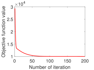
First we analyze the convergence property of the optimization parts in Algorithm 1 (or Algorithm 2). Thanks to the superiority of the APG, it can guarantee Eq.(8) (or Eq.(12)) to converge to a global optimum and have the convergence rate such that (𝐖t)(𝐖)𝒪(1/t2)subscript𝐖𝑡superscript𝐖𝒪1superscript𝑡2\mathcal{F}(\mathbf{W}_{t})-\mathcal{F}(\mathbf{W}^{*})\leq\mathcal{O}(1/t^{2}) (or (𝐀t)(𝐀)𝒪(1/t2)subscript𝐀𝑡superscript𝐀𝒪1superscript𝑡2\mathcal{F}(\mathbf{A}_{t})-\mathcal{F}(\mathbf{A}^{*})\leq\mathcal{O}(1/t^{2})), where 𝐖superscript𝐖\mathbf{W}^{*} (or 𝐀superscript𝐀\mathbf{A}^{*}) is an optimal solution of Eq.(8) (or Eq.(12)). In other words, to get an ϵitalic-ϵ\epsilon tolerance accurate solution, it needs 𝒪(1/ϵ)𝒪1italic-ϵ\mathcal{O}(1/\sqrt{\epsilon}) iteration rounds.

Then, the computational time complexity of Algorithm 1 is analyzed as follows. In step 3, the computation of the Lipschitz constant needs 𝒪(nm2+nl2)𝒪𝑛superscript𝑚2𝑛superscript𝑙2\mathcal{O}(nm^{2}+nl^{2}). In each iteration, step 5, which needs 𝒪(nm2+m2l+nml2)𝒪𝑛superscript𝑚2superscript𝑚2𝑙𝑛𝑚superscript𝑙2\mathcal{O}(nm^{2}+m^{2}l+nml^{2}), is the most expensive. Regularly, for an m×l𝑚𝑙m\times l matrix, the computation of the singular value decomposition (SVD) requires 𝒪(mlmin(m,l))𝒪𝑚𝑙min𝑚𝑙\mathcal{O}(ml{\rm min}(m,l)) [15]. Since it usually meets mlmuch-greater-than𝑚𝑙m\gg l in multi-label classification, step 6 requires 𝒪(ml2)𝒪𝑚superscript𝑙2\mathcal{O}(ml^{2}). Besides, it needs 𝒪(ml)𝒪𝑚𝑙\mathcal{O}(ml) in step 8. Consequently, for Algorithm 1, the overall computational time complexity is 𝒪((nm2+m2l+nml2)/ϵ)𝒪𝑛superscript𝑚2superscript𝑚2𝑙𝑛𝑚superscript𝑙2italic-ϵ\mathcal{O}((nm^{2}+m^{2}l+nml^{2})/\sqrt{\epsilon}) to get an ϵitalic-ϵ\epsilon tolerance accurate solution.

Here the computational time complexity of Algorithm 2 is analyzed. In step 3, the computation of the Lipschitz constant leads to 𝒪(n3+nl2)𝒪superscript𝑛3𝑛superscript𝑙2\mathcal{O}(n^{3}+nl^{2}). In each iteration, step 5, which needs 𝒪(n3+n2l2)𝒪superscript𝑛3superscript𝑛2superscript𝑙2\mathcal{O}(n^{3}+n^{2}l^{2}), is the most expensive. It leads to 𝒪(nl2)𝒪𝑛superscript𝑙2\mathcal{O}(nl^{2}) in step 6. Besides, it needs 𝒪(nl)𝒪𝑛𝑙\mathcal{O}(nl) in step 8. Hence, for Algorithm 2, the overall computational time complexity is 𝒪((n3+n2l2)/ϵ)𝒪superscript𝑛3superscript𝑛2superscript𝑙2italic-ϵ\mathcal{O}((n^{3}+n^{2}l^{2})/\sqrt{\epsilon}) to get an ϵitalic-ϵ\epsilon tolerance accurate solution.

Furthermore, based on the computational complexity analysis, it can be observed that when the number of instances (i.e. n𝑛n) or labels (i.e. l𝑙l) is large, a stochastic variant of our method might be a better choice for efficient training.

5 Experiments

5.1 Datasets and settings

In our experiments, we conduct comparative experiments on 10 widely-used multi-label benchmark datasets, which covers a broad range of sizes and domains. Different datasets might demonstrate diverse label correlations and input-output relationships, which poses great challenges for multi-label classification (MLC) approaches. The statistics of the experimental datasets are summarized in Table 1. For each dataset, 60% is randomly split for training, and the rest 40% is for testing. Besides, ten independent experiments are repeated for the reduction of statistical variability.

Table 1: Statistics of the experimental datasets. (“Cardinality” indicates the average number of labels per example. “Density” normalizes the “Cardinality” by the number of possible labels. “URL” indicates the source URL of the dataset.)
Dataset #Instance #Feature #Label Cardinality Density Domain URL111URL 1: http://mulan.sourceforge.net/datasets-mlc.html
emotions 593 72 6 1.869 0.311 music URL 1
image 2000 294 5 1.240 0.248 image URL 2
scene 2407 294 6 1.074 0.179 image URL 1
yeast 2417 103 14 4.237 0.303 biology URL 1
enron 1702 1001 53 3.378 0.064 text URL 1
arts 5000 462 26 1.636 0.063 text URL 1
education 5000 550 33 1.461 0.044 text URL 1
recreation 5000 606 22 1.423 0.065 text URL 1
science 5000 743 40 1.451 0.036 text URL 1
business 5000 438 30 1.588 0.053 text URL 1
11footnotetext: URL 2: http://palm.seu.edu.cn/zhangml/

We compare the proposed approach RBRL with the following state-of-the-art baseline approaches for MLC. For each baseline approach, the setting and search range of the hyper-parameters are employed by recommendations of the original literature.

  1. (1)

    RBRL222source code: https://github.com/GuoqiangWoodrowWu/RBRL. It is our proposed approach, where the hyper-parameters λ1,λ2,λ3subscript𝜆1subscript𝜆2subscript𝜆3\lambda_{1},\lambda_{2},\lambda_{3} are tuned in {104,103,,102}superscript104superscript103superscript102\{10^{-4},10^{-3},...,10^{2}\}.

  2. (2)

    Rank-SVM333source code: http://palm.seu.edu.cn/zhangml/ [9]. It is an adaption of the maximum margin strategy for MLC.

  3. (3)

    Rank-SVMz444source code: http://computer.njnu.edu.cn/Lab/LABIC/LABIC_Software.html [48]. It is a variant method of Rank-SVM for MLC.

  4. (4)

    BR [2]. It converts MLC task into many independent binary classification problems.

  5. (5)

    ML-kNN [56]. It is an adaption of the lazy learning kNN classifier for MLC.

  6. (6)

    CLR [13]. It converts MLC task into the pairwise label ranking problem.

  7. (7)

    RAKEL [37]. It converts MLC task into an ensemble of multi-class classification problems.

  8. (8)

    CPNL [42]. It is a recent approach which presents a cost-sensitive loss to address the class-imbalance issue and boosts the performance by exploitations of negative and positive label correlations.

  9. (9)

    MLFE555source code: http://palm.seu.edu.cn/zhangml/ [58]. It is also a recent approach that leverages the structural information of the feature space to enrich the labeling information.

Motivated by [18, 42], which concludes that the linear model is good enough for high dimensional feature problems, we test the performance of the linear model on the last six datasets and evaluate the kernel model on the first four datasets (i.e., emotions, image, scene and yeast).

For the last six datasets, LIBLINEAR [10] is employed as the base learner for BR, CLR and RAKEL, where the hyper-parameter C𝐶C is tuned in {104,103,,104}superscript104superscript103superscript104\{10^{-4},10^{-3},...,10^{4}\}. The commonly-used MULAN [38] implementations are adopted for BR, ML-kNN, CLR, and RAKEL. Besides, thanks to the publicly available, other approaches employ the original implementations from the corresponding source code website. Moreover, for the sake of fairness, Rank-SVM and Rank-SVMz adopt the linear kernel, and we employ the linear RBRL.

For the first four datasets, LIBSVM [4] is employed as the base learner for BR, CLR and RAKEL, where the hyper-parameter C𝐶C is tuned in {104,103,,104}superscript104superscript103superscript104\{10^{-4},10^{-3},...,10^{4}\}. Although other kernel functions (such as polynomial kernel function) can be used, we adopt the RBF kernel k(𝐱i,𝐱j)=exp(γ𝐱i𝐱j2)𝑘subscript𝐱𝑖subscript𝐱𝑗𝑒𝑥𝑝𝛾superscriptnormsubscript𝐱𝑖subscript𝐱𝑗2k(\mathbf{x}_{i},\mathbf{x}_{j})=exp(-\gamma\|\mathbf{x}_{i}-\mathbf{x}_{j}\|^{2}) due to its wide applications in practice, and the kernel parameter γ𝛾\gamma is set to be 1/m1𝑚1/m (m𝑚m is the feature number). Besides, Rank-SVM, Rank-SVMz and our proposed approach RBRL also use the RBF kernel for a fair comparison.

Furthermore, for each compared approach, its hyper-parameters are selected via fivefold cross-validation on the training set. For convenience, Table 2 summarizes the hyper-parameters setup for each compared approach in detail.

Table 2: Summary of the hyper-parameters setup for each compared approach
Approach Hyper-parameters setup Citation
RBRL λ1,λ2,λ3={104,103,,102}subscript𝜆1subscript𝜆2subscript𝜆3superscript104superscript103superscript102\lambda_{1},\lambda_{2},\lambda_{3}=\{10^{-4},10^{-3},...,10^{2}\} N/A
Rank-SVM C={104,103,,104}𝐶superscript104superscript103superscript104C=\{10^{-4},10^{-3},...,10^{4}\} [9]
Rank-SVMz C={104,103,,104}𝐶superscript104superscript103superscript104C=\{10^{-4},10^{-3},...,10^{4}\} [48]
BR C={104,103,,104}𝐶superscript104superscript103superscript104C=\{10^{-4},10^{-3},...,10^{4}\} [2]
ML-kNN k={4,6,,16}𝑘4616k=\{4,6,...,16\} [56]
CLR C={104,103,,104}𝐶superscript104superscript103superscript104C=\{10^{-4},10^{-3},...,10^{4}\} [13]
RAKEL (1) m=10,k=l/2formulae-sequence𝑚10𝑘𝑙2m=10,k=l/2 (2) m=2l,k=3formulae-sequence𝑚2𝑙𝑘3m=2l,k=3 [37]
C={104,103,,104}𝐶superscript104superscript103superscript104C=\{10^{-4},10^{-3},...,10^{4}\}
CPNL β=0.5𝛽0.5\beta=0.5, k=3𝑘3k=3 [42]
λ1,λ2,λ3={104,103,,102}subscript𝜆1subscript𝜆2subscript𝜆3superscript104superscript103superscript102\lambda_{1},\lambda_{2},\lambda_{3}=\{10^{-4},10^{-3},...,10^{2}\}
MLFE β1={1,2,,10}subscript𝛽11210\beta_{1}=\{1,2,...,10\}, β2={1,10,15}subscript𝛽211015\beta_{2}=\{1,10,15\} [58]
β3={1,10}subscript𝛽3110\beta_{3}=\{1,10\}

5.2 Evaluation metrics

Given a testing set 𝒟t={𝐱i,𝐲i}i=1ntsubscript𝒟𝑡superscriptsubscriptsubscript𝐱𝑖subscript𝐲𝑖𝑖1subscript𝑛𝑡\mathcal{D}_{t}=\{\mathbf{x}_{i},\mathbf{y}_{i}\}_{i=1}^{n_{t}} and the family of l𝑙l learned functions F={f1,f2,,fl}𝐹subscript𝑓1subscript𝑓2subscript𝑓𝑙F=\{f_{1},f_{2},...,f_{l}\}, where 𝐲i{1,+1}lsubscript𝐲𝑖superscript11𝑙\mathbf{y}_{i}\in\{-1,+1\}^{l} is the ground-truth labels of 𝐱isubscript𝐱𝑖\mathbf{x}_{i}. Besides, H={h1,h2,,hl}𝐻subscript1subscript2subscript𝑙H=\{h_{1},h_{2},...,h_{l}\} denotes the multi-label classifier. In this paper, we employ the following six commonly evaluation metrics [57, 45], which includes three classification-based metrics (i.e., Hamming Loss, Subset Accuracy and F1-Example) and three ranking-based metrics (i.e., Ranking Loss, Coverage and Average Precision).

  1. (1)

    Hamming Loss (Hal): It measures the fraction of misclassified example-label pairs.

    Hal=1ntli=1ntj=1l[[hj(𝐱i)yij]]Hal1subscript𝑛𝑡𝑙superscriptsubscript𝑖1subscript𝑛𝑡superscriptsubscript𝑗1𝑙delimited-[]delimited-[]subscript𝑗subscript𝐱𝑖subscript𝑦𝑖𝑗{\rm Hal}=\frac{1}{n_{t}l}\sum_{i=1}^{n_{t}}\sum_{j=1}^{l}[\![h_{j}(\mathbf{x}_{i})\neq y_{ij}]\!] (34)
  2. (2)

    Subset Accuracy (Sa): It measures the fraction that the predicted label subset and the ground-truth label subset are the same.

    Sa=1nti=1nt[[H(𝐱i)=𝐲i]]Sa1subscript𝑛𝑡superscriptsubscript𝑖1subscript𝑛𝑡delimited-[]delimited-[]𝐻subscript𝐱𝑖subscript𝐲𝑖{\rm Sa}=\frac{1}{n_{t}}\sum_{i=1}^{n_{t}}[\![H(\mathbf{x}_{i})=\mathbf{y}_{i}]\!] (35)
  3. (3)

    F1-Example (F1e): It is the average F1 measure that is the harmonic mean of recall and precision over each instance.

    F1e=1nti=1nt2|Pi+Yi+||Pi+|+|Yi+|F1e1subscript𝑛𝑡superscriptsubscript𝑖1subscript𝑛𝑡2superscriptsubscript𝑃𝑖superscriptsubscript𝑌𝑖superscriptsubscript𝑃𝑖superscriptsubscript𝑌𝑖{\rm F1e}=\frac{1}{n_{t}}\sum_{i=1}^{n_{t}}\frac{2|P_{i}^{+}\cap Y_{i}^{+}|}{|P_{i}^{+}|+|Y_{i}^{+}|} (36)

    where Yi+superscriptsubscript𝑌𝑖Y_{i}^{+} (or Yisuperscriptsubscript𝑌𝑖Y_{i}^{-}) denotes the index set of the ground-truth relevant (or irrelevant) labels associated with 𝐱isubscript𝐱𝑖\mathbf{x}_{i}, and Pi+superscriptsubscript𝑃𝑖P_{i}^{+} (or Pisuperscriptsubscript𝑃𝑖P_{i}^{-}) denotes the index set of the predicted relevant (or irrelevant) labels associated with 𝐱isubscript𝐱𝑖\mathbf{x}_{i}.

  4. (4)

    Ranking Loss (Ral): It measures the average fraction of the label pairs that an irrelevant label ranks higher than a relevant label over each instance.

    Ral=1nti=1nt|SetRi||Yi+||Yi|Ral1subscript𝑛𝑡superscriptsubscript𝑖1subscript𝑛𝑡𝑆𝑒𝑡subscript𝑅𝑖superscriptsubscript𝑌𝑖superscriptsubscript𝑌𝑖{\rm Ral}=\frac{1}{n_{t}}\sum_{i=1}^{n_{t}}\frac{|SetR_{i}|}{|Y_{i}^{+}||Y_{i}^{-}|} (37)

    where SetRi={(p,q)|fp(𝐱i)fq(𝐱i),(p,q)Yi+×Yi}𝑆𝑒𝑡subscript𝑅𝑖conditional-set𝑝𝑞formulae-sequencesubscript𝑓𝑝subscript𝐱𝑖subscript𝑓𝑞subscript𝐱𝑖𝑝𝑞superscriptsubscript𝑌𝑖superscriptsubscript𝑌𝑖SetR_{i}=\{(p,q)|f_{p}(\mathbf{x}_{i})\leq f_{q}(\mathbf{x}_{i}),(p,q)\in Y_{i}^{+}\times Y_{i}^{-}\}.

  5. (5)

    Coverage (Cov): It measures how many steps are needed to cover all relevant labels averagely based on the predicted ranking label list. Besides, this metric is normalized in [0,1]01[0,1] by the number of possible labels here.

    Cov=1l(1nti=1ntmaxjYi+rankF(𝐱i,j)1)Cov1𝑙1subscript𝑛𝑡superscriptsubscript𝑖1subscript𝑛𝑡subscript𝑗superscriptsubscript𝑌𝑖𝑟𝑎𝑛subscript𝑘𝐹subscript𝐱𝑖𝑗1{\rm Cov}=\frac{1}{l}(\frac{1}{n_{t}}\sum_{i=1}^{n_{t}}\mathop{\max}_{j\in Y_{i}^{+}}rank_{F}(\mathbf{x}_{i},j)-1) (38)

    where rankF(𝐱i,j)𝑟𝑎𝑛subscript𝑘𝐹subscript𝐱𝑖𝑗rank_{F}(\mathbf{x}_{i},j) stands for the rank of label j𝑗j in the ranking list based on F(𝐱i)𝐹subscript𝐱𝑖F(\mathbf{x}_{i}) which is sorted in descending order.

  6. (6)

    Average Precision (Ap): It measures the average fraction of relevant labels ranked higher than a specific relevant label.

    Ap=1nti=1nt1|Yi+|jYi+|SetPij|rankF(𝐱i,j)Ap1subscript𝑛𝑡superscriptsubscript𝑖1subscript𝑛𝑡1superscriptsubscript𝑌𝑖subscript𝑗superscriptsubscript𝑌𝑖𝑆𝑒𝑡subscript𝑃𝑖𝑗𝑟𝑎𝑛subscript𝑘𝐹subscript𝐱𝑖𝑗{\rm Ap}=\frac{1}{n_{t}}\sum_{i=1}^{n_{t}}\frac{1}{|Y_{i}^{+}|}\sum_{j\in Y_{i}^{+}}\frac{|SetP_{ij}|}{rank_{F}(\mathbf{x}_{i},j)} (39)

    where SetPij={kYi+|rankF(𝐱i,k)rankF(𝐱i,j)}𝑆𝑒𝑡subscript𝑃𝑖𝑗conditional-set𝑘superscriptsubscript𝑌𝑖𝑟𝑎𝑛subscript𝑘𝐹subscript𝐱𝑖𝑘𝑟𝑎𝑛subscript𝑘𝐹subscript𝐱𝑖𝑗SetP_{ij}=\{k\in Y_{i}^{+}|rank_{F}(\mathbf{x}_{i},k)\leq rank_{F}(\mathbf{x}_{i},j)\}.

For Sa, F1e and Ap, the larger the value, the better performance of the multi-label classifier; while for the others, the smaller the value, the better performance of the multi-label classifier.

5.3 Experiments Results

5.3.1 Performance Comparison

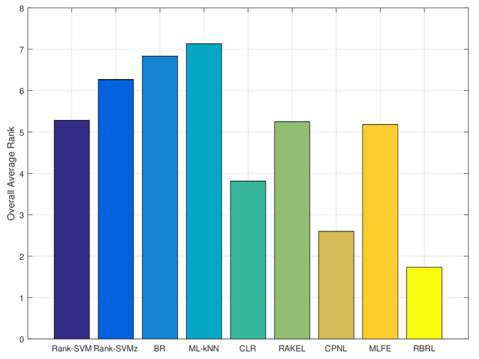
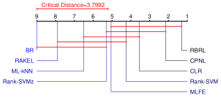
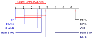
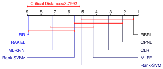
The multi-label prediction results of the proposed RBRL and the comparison with several state-of-the-art approaches are summarized in Table 3. Besides, the average ranks of these compared approaches in terms of each metric on all the datasets are summarized in Table 4. Intuitively, Figure 1 shows the overall average ranks of these compared approaches over all the metrics.

Table 3: Experimental results of each benchmark approach (mean ±plus-or-minus\pm std) on 10 multi-label datasets. ()absent\downarrow(\uparrow) indicates the smaller(larger) the better. Best results are highlighted in bold.
Metric Rank-SVM Rank-SVMz BR ML-kNN CLR RAKEL CPNL MLFE RBRL
emotions Hal (\downarrow) 0.189±0.008plus-or-minus0.1890.0080.189\pm 0.008 0.201±0.008plus-or-minus0.2010.0080.201\pm 0.008 0.183±0.009plus-or-minus0.1830.0090.183\pm 0.009 0.200±0.013plus-or-minus0.2000.0130.200\pm 0.013 0.182±0.008plus-or-minus0.1820.0080.182\pm 0.008 0.177±0.008plus-or-minus0.1770.008\bf 0.177\pm 0.008 0.183±0.009plus-or-minus0.1830.0090.183\pm 0.009 0.186±0.009plus-or-minus0.1860.0090.186\pm 0.009 0.181±0.012plus-or-minus0.1810.0120.181\pm 0.012
Sa (\uparrow) 0.291±0.025plus-or-minus0.2910.0250.291\pm 0.025 0.292±0.024plus-or-minus0.2920.0240.292\pm 0.024 0.313±0.015plus-or-minus0.3130.0150.313\pm 0.015 0.285±0.028plus-or-minus0.2850.0280.285\pm 0.028 0.318±0.013plus-or-minus0.3180.0130.318\pm 0.013 0.356±0.028plus-or-minus0.3560.028\bf 0.356\pm 0.028 0.324±0.035plus-or-minus0.3240.0350.324\pm 0.035 0.291±0.035plus-or-minus0.2910.0350.291\pm 0.035 0.334±0.032plus-or-minus0.3340.0320.334\pm 0.032
F1e (\uparrow) 0.645±0.020plus-or-minus0.6450.0200.645\pm 0.020 0.675±0.012plus-or-minus0.6750.0120.675\pm 0.012 0.620±0.020plus-or-minus0.6200.0200.620\pm 0.020 0.605±0.039plus-or-minus0.6050.0390.605\pm 0.039 0.624±0.019plus-or-minus0.6240.0190.624\pm 0.019 0.679±0.019plus-or-minus0.6790.0190.679\pm 0.019 0.684±0.019plus-or-minus0.6840.019\bf 0.684\pm 0.019 0.621±0.021plus-or-minus0.6210.0210.621\pm 0.021 0.666±0.022plus-or-minus0.6660.0220.666\pm 0.022
Ral (\downarrow) 0.155±0.009plus-or-minus0.1550.0090.155\pm 0.009 0.149±0.008plus-or-minus0.1490.0080.149\pm 0.008 0.246±0.015plus-or-minus0.2460.0150.246\pm 0.015 0.169±0.016plus-or-minus0.1690.0160.169\pm 0.016 0.149±0.014plus-or-minus0.1490.0140.149\pm 0.014 0.192±0.017plus-or-minus0.1920.0170.192\pm 0.017 0.139±0.010plus-or-minus0.1390.0100.139\pm 0.010 0.142±0.011plus-or-minus0.1420.0110.142\pm 0.011 0.138±0.011plus-or-minus0.1380.011\bf 0.138\pm 0.011
Cov (\downarrow) 0.294±0.011plus-or-minus0.2940.0110.294\pm 0.011 0.291±0.008plus-or-minus0.2910.0080.291\pm 0.008 0.386±0.017plus-or-minus0.3860.0170.386\pm 0.017 0.306±0.016plus-or-minus0.3060.0160.306\pm 0.016 0.283±0.012plus-or-minus0.2830.0120.283\pm 0.012 0.338±0.014plus-or-minus0.3380.0140.338\pm 0.014 0.277±0.010plus-or-minus0.2770.010\bf 0.277\pm 0.010 0.282±0.013plus-or-minus0.2820.0130.282\pm 0.013 0.277±0.010plus-or-minus0.2770.010\bf 0.277\pm 0.010
Ap (\uparrow) 0.808±0.010plus-or-minus0.8080.0100.808\pm 0.010 0.819±0.012plus-or-minus0.8190.0120.819\pm 0.012 0.760±0.015plus-or-minus0.7600.0150.760\pm 0.015 0.796±0.016plus-or-minus0.7960.0160.796\pm 0.016 0.813±0.014plus-or-minus0.8130.0140.813\pm 0.014 0.801±0.015plus-or-minus0.8010.0150.801\pm 0.015 0.828±0.010plus-or-minus0.8280.010\bf 0.828\pm 0.010 0.822±0.012plus-or-minus0.8220.0120.822\pm 0.012 0.828±0.014plus-or-minus0.8280.014\bf 0.828\pm 0.014
image Hal (\downarrow) 0.161±0.005plus-or-minus0.1610.0050.161\pm 0.005 0.177±0.010plus-or-minus0.1770.0100.177\pm 0.010 0.156±0.006plus-or-minus0.1560.0060.156\pm 0.006 0.175±0.007plus-or-minus0.1750.0070.175\pm 0.007 0.157±0.006plus-or-minus0.1570.0060.157\pm 0.006 0.154±0.006plus-or-minus0.1540.0060.154\pm 0.006 0.150±0.006plus-or-minus0.1500.0060.150\pm 0.006 0.156±0.007plus-or-minus0.1560.0070.156\pm 0.007 0.149±0.005plus-or-minus0.1490.005\bf 0.149\pm 0.005
Sa (\uparrow) 0.451±0.018plus-or-minus0.4510.0180.451\pm 0.018 0.411±0.025plus-or-minus0.4110.0250.411\pm 0.025 0.482±0.018plus-or-minus0.4820.0180.482\pm 0.018 0.393±0.024plus-or-minus0.3930.0240.393\pm 0.024 0.477±0.016plus-or-minus0.4770.0160.477\pm 0.016 0.527±0.013plus-or-minus0.5270.0130.527\pm 0.013 0.533±0.017plus-or-minus0.5330.0170.533\pm 0.017 0.463±0.015plus-or-minus0.4630.0150.463\pm 0.015 0.552±0.011plus-or-minus0.5520.011\bf 0.552\pm 0.011
F1e (\uparrow) 0.631±0.016plus-or-minus0.6310.0160.631\pm 0.016 0.670±0.022plus-or-minus0.6700.0220.670\pm 0.022 0.623±0.014plus-or-minus0.6230.0140.623\pm 0.014 0.503±0.026plus-or-minus0.5030.0260.503\pm 0.026 0.627±0.014plus-or-minus0.6270.0140.627\pm 0.014 0.680±0.012plus-or-minus0.6800.0120.680\pm 0.012 0.698±0.012plus-or-minus0.6980.012\bf 0.698\pm 0.012 0.593±0.014plus-or-minus0.5930.0140.593\pm 0.014 0.688±0.012plus-or-minus0.6880.0120.688\pm 0.012
Ral (\downarrow) 0.143±0.008plus-or-minus0.1430.0080.143\pm 0.008 0.142±0.014plus-or-minus0.1420.0140.142\pm 0.014 0.220±0.012plus-or-minus0.2200.0120.220\pm 0.012 0.180±0.010plus-or-minus0.1800.0100.180\pm 0.010 0.144±0.006plus-or-minus0.1440.0060.144\pm 0.006 0.173±0.009plus-or-minus0.1730.0090.173\pm 0.009 0.132±0.006plus-or-minus0.1320.006\bf 0.132\pm 0.006 0.142±0.007plus-or-minus0.1420.0070.142\pm 0.007 0.133±0.007plus-or-minus0.1330.0070.133\pm 0.007
Cov (\downarrow) 0.171±0.008plus-or-minus0.1710.0080.171\pm 0.008 0.170±0.012plus-or-minus0.1700.0120.170\pm 0.012 0.227±0.008plus-or-minus0.2270.0080.227\pm 0.008 0.198±0.009plus-or-minus0.1980.0090.198\pm 0.009 0.168±0.007plus-or-minus0.1680.0070.168\pm 0.007 0.191±0.007plus-or-minus0.1910.0070.191\pm 0.007 0.157±0.006plus-or-minus0.1570.006\bf 0.157\pm 0.006 0.165±0.006plus-or-minus0.1650.0060.165\pm 0.006 0.160±0.006plus-or-minus0.1600.0060.160\pm 0.006
Ap (\uparrow) 0.823±0.010plus-or-minus0.8230.0100.823\pm 0.010 0.826±0.016plus-or-minus0.8260.0160.826\pm 0.016 0.772±0.011plus-or-minus0.7720.0110.772\pm 0.011 0.786±0.009plus-or-minus0.7860.0090.786\pm 0.009 0.826±0.006plus-or-minus0.8260.0060.826\pm 0.006 0.813±0.008plus-or-minus0.8130.0080.813\pm 0.008 0.839±0.007plus-or-minus0.8390.007\bf 0.839\pm 0.007 0.826±0.008plus-or-minus0.8260.0080.826\pm 0.008 0.836±0.008plus-or-minus0.8360.0080.836\pm 0.008
scene Hal (\downarrow) 0.092±0.005plus-or-minus0.0920.0050.092\pm 0.005 0.113±0.004plus-or-minus0.1130.0040.113\pm 0.004 0.077±0.002plus-or-minus0.0770.0020.077\pm 0.002 0.091±0.003plus-or-minus0.0910.0030.091\pm 0.003 0.078±0.002plus-or-minus0.0780.0020.078\pm 0.002 0.075±0.004plus-or-minus0.0750.0040.075\pm 0.004 0.077±0.003plus-or-minus0.0770.0030.077\pm 0.003 0.083±0.003plus-or-minus0.0830.0030.083\pm 0.003 0.073±0.004plus-or-minus0.0730.004\bf 0.073\pm 0.004
Sa (\uparrow) 0.563±0.018plus-or-minus0.5630.0180.563\pm 0.018 0.500±0.015plus-or-minus0.5000.0150.500\pm 0.015 0.655±0.009plus-or-minus0.6550.0090.655\pm 0.009 0.615±0.019plus-or-minus0.6150.0190.615\pm 0.019 0.650±0.010plus-or-minus0.6500.0100.650\pm 0.010 0.696±0.014plus-or-minus0.6960.0140.696\pm 0.014 0.699±0.014plus-or-minus0.6990.0140.699\pm 0.014 0.617±0.009plus-or-minus0.6170.0090.617\pm 0.009 0.735±0.013plus-or-minus0.7350.013\bf 0.735\pm 0.013
F1e (\uparrow) 0.664±0.015plus-or-minus0.6640.0150.664\pm 0.015 0.756±0.005plus-or-minus0.7560.0050.756\pm 0.005 0.717±0.010plus-or-minus0.7170.0100.717\pm 0.010 0.678±0.022plus-or-minus0.6780.0220.678\pm 0.022 0.718±0.011plus-or-minus0.7180.0110.718\pm 0.011 0.756±0.012plus-or-minus0.7560.0120.756\pm 0.012 0.802±0.009plus-or-minus0.8020.0090.802\pm 0.009 0.685±0.010plus-or-minus0.6850.0100.685\pm 0.010 0.803±0.010plus-or-minus0.8030.010\bf 0.803\pm 0.010
Ral (\downarrow) 0.065±0.005plus-or-minus0.0650.0050.065\pm 0.005 0.072±0.005plus-or-minus0.0720.0050.072\pm 0.005 0.128±0.006plus-or-minus0.1280.0060.128\pm 0.006 0.083±0.006plus-or-minus0.0830.0060.083\pm 0.006 0.061±0.003plus-or-minus0.0610.0030.061\pm 0.003 0.087±0.005plus-or-minus0.0870.0050.087\pm 0.005 0.059±0.003plus-or-minus0.0590.0030.059\pm 0.003 0.063±0.003plus-or-minus0.0630.0030.063\pm 0.003 0.058±0.004plus-or-minus0.0580.004\bf 0.058\pm 0.004
Cov (\downarrow) 0.068±0.004plus-or-minus0.0680.0040.068\pm 0.004 0.075±0.004plus-or-minus0.0750.0040.075\pm 0.004 0.119±0.004plus-or-minus0.1190.0040.119\pm 0.004 0.084±0.005plus-or-minus0.0840.0050.084\pm 0.005 0.064±0.003plus-or-minus0.0640.0030.064\pm 0.003 0.089±0.005plus-or-minus0.0890.0050.089\pm 0.005 0.064±0.002plus-or-minus0.0640.0020.064\pm 0.002 0.067±0.003plus-or-minus0.0670.0030.067\pm 0.003 0.062±0.003plus-or-minus0.0620.003\bf 0.062\pm 0.003
Ap (\uparrow) 0.882±0.008plus-or-minus0.8820.0080.882\pm 0.008 0.874±0.007plus-or-minus0.8740.0070.874\pm 0.007 0.834±0.006plus-or-minus0.8340.0060.834\pm 0.006 0.858±0.007plus-or-minus0.8580.0070.858\pm 0.007 0.887±0.004plus-or-minus0.8870.0040.887\pm 0.004 0.875±0.006plus-or-minus0.8750.0060.875\pm 0.006 0.893±0.006plus-or-minus0.8930.0060.893\pm 0.006 0.885±0.005plus-or-minus0.8850.0050.885\pm 0.005 0.895±0.006plus-or-minus0.8950.006\bf 0.895\pm 0.006
yeast Hal (\downarrow) 0.203±0.004plus-or-minus0.2030.0040.203\pm 0.004 0.207±0.007plus-or-minus0.2070.0070.207\pm 0.007 0.188±0.003plus-or-minus0.1880.0030.188\pm 0.003 0.195±0.003plus-or-minus0.1950.0030.195\pm 0.003 0.188±0.003plus-or-minus0.1880.0030.188\pm 0.003 0.195±0.003plus-or-minus0.1950.0030.195\pm 0.003 0.192±0.004plus-or-minus0.1920.0040.192\pm 0.004 0.194±0.004plus-or-minus0.1940.0040.194\pm 0.004 0.187±0.004plus-or-minus0.1870.004\bf 0.187\pm 0.004
Sa (\uparrow) 0.156±0.012plus-or-minus0.1560.0120.156\pm 0.012 0.179±0.009plus-or-minus0.1790.0090.179\pm 0.009 0.190±0.009plus-or-minus0.1900.0090.190\pm 0.009 0.177±0.013plus-or-minus0.1770.0130.177\pm 0.013 0.194±0.009plus-or-minus0.1940.0090.194\pm 0.009 0.248±0.006plus-or-minus0.2480.006\bf 0.248\pm 0.006 0.179±0.006plus-or-minus0.1790.0060.179\pm 0.006 0.172±0.014plus-or-minus0.1720.0140.172\pm 0.014 0.192±0.009plus-or-minus0.1920.0090.192\pm 0.009
F1e (\uparrow) 0.632±0.007plus-or-minus0.6320.0070.632\pm 0.007 0.643±0.009plus-or-minus0.6430.0090.643\pm 0.009 0.623±0.006plus-or-minus0.6230.0060.623\pm 0.006 0.615±0.012plus-or-minus0.6150.0120.615\pm 0.012 0.625±0.006plus-or-minus0.6250.0060.625\pm 0.006 0.647±0.005plus-or-minus0.6470.005\bf 0.647\pm 0.005 0.630±0.007plus-or-minus0.6300.0070.630\pm 0.007 0.607±0.011plus-or-minus0.6070.0110.607\pm 0.011 0.628±0.007plus-or-minus0.6280.0070.628\pm 0.007
Ral (\downarrow) 0.170±0.005plus-or-minus0.1700.0050.170\pm 0.005 0.172±0.005plus-or-minus0.1720.0050.172\pm 0.005 0.308±0.008plus-or-minus0.3080.0080.308\pm 0.008 0.170±0.005plus-or-minus0.1700.0050.170\pm 0.005 0.158±0.005plus-or-minus0.1580.0050.158\pm 0.005 0.244±0.008plus-or-minus0.2440.0080.244\pm 0.008 0.158±0.006plus-or-minus0.1580.0060.158\pm 0.006 0.166±0.005plus-or-minus0.1660.0050.166\pm 0.005 0.157±0.005plus-or-minus0.1570.005\bf 0.157\pm 0.005
Cov (\downarrow) 0.446±0.006plus-or-minus0.4460.0060.446\pm 0.006 0.458±0.006plus-or-minus0.4580.0060.458\pm 0.006 0.627±0.007plus-or-minus0.6270.0070.627\pm 0.007 0.451±0.009plus-or-minus0.4510.0090.451\pm 0.009 0.436±0.006plus-or-minus0.4360.006\bf 0.436\pm 0.006 0.543±0.005plus-or-minus0.5430.0050.543\pm 0.005 0.445±0.006plus-or-minus0.4450.0060.445\pm 0.006 0.452±0.006plus-or-minus0.4520.0060.452\pm 0.006 0.436±0.007plus-or-minus0.4360.007\bf 0.436\pm 0.007
Ap (\uparrow) 0.755±0.005plus-or-minus0.7550.0050.755\pm 0.005 0.765±0.006plus-or-minus0.7650.0060.765\pm 0.006 0.680±0.007plus-or-minus0.6800.0070.680\pm 0.007 0.762±0.005plus-or-minus0.7620.0050.762\pm 0.005 0.773±0.008plus-or-minus0.7730.0080.773\pm 0.008 0.727±0.004plus-or-minus0.7270.0040.727\pm 0.004 0.775±0.009plus-or-minus0.7750.0090.775\pm 0.009 0.769±0.008plus-or-minus0.7690.0080.769\pm 0.008 0.777±0.005plus-or-minus0.7770.005\bf 0.777\pm 0.005
enron Hal (\downarrow) 0.051±0.003plus-or-minus0.0510.0030.051\pm 0.003 0.061±0.002plus-or-minus0.0610.0020.061\pm 0.002 0.052±0.001plus-or-minus0.0520.0010.052\pm 0.001 0.054±0.001plus-or-minus0.0540.0010.054\pm 0.001 0.050±0.001plus-or-minus0.0500.0010.050\pm 0.001 0.052±0.001plus-or-minus0.0520.0010.052\pm 0.001 0.049±0.001plus-or-minus0.0490.0010.049\pm 0.001 0.046±0.001plus-or-minus0.0460.001\bf 0.046\pm 0.001 0.046±0.001plus-or-minus0.0460.001\bf 0.046\pm 0.001
Sa (\uparrow) 0.119±0.033plus-or-minus0.1190.0330.119\pm 0.033 0.060±0.007plus-or-minus0.0600.0070.060\pm 0.007 0.128±0.013plus-or-minus0.1280.0130.128\pm 0.013 0.057±0.015plus-or-minus0.0570.0150.057\pm 0.015 0.131±0.014plus-or-minus0.1310.0140.131\pm 0.014 0.154±0.010plus-or-minus0.1540.010\bf 0.154\pm 0.010 0.128±0.006plus-or-minus0.1280.0060.128\pm 0.006 0.124±0.014plus-or-minus0.1240.0140.124\pm 0.014 0.137±0.014plus-or-minus0.1370.0140.137\pm 0.014
F1e (\uparrow) 0.563±0.026plus-or-minus0.5630.0260.563\pm 0.026 0.463±0.022plus-or-minus0.4630.0220.463\pm 0.022 0.529±0.010plus-or-minus0.5290.0100.529\pm 0.010 0.401±0.029plus-or-minus0.4010.0290.401\pm 0.029 0.552±0.011plus-or-minus0.5520.0110.552\pm 0.011 0.551±0.009plus-or-minus0.5510.0090.551\pm 0.009 0.585±0.007plus-or-minus0.5850.007\bf 0.585\pm 0.007 0.538±0.012plus-or-minus0.5380.0120.538\pm 0.012 0.569±0.009plus-or-minus0.5690.0090.569\pm 0.009
Ral (\downarrow) 0.081±0.008plus-or-minus0.0810.0080.081\pm 0.008 0.098±0.005plus-or-minus0.0980.0050.098\pm 0.005 0.298±0.007plus-or-minus0.2980.0070.298\pm 0.007 0.096±0.003plus-or-minus0.0960.0030.096\pm 0.003 0.071±0.003plus-or-minus0.0710.003\bf 0.071\pm 0.003 0.208±0.006plus-or-minus0.2080.0060.208\pm 0.006 0.078±0.003plus-or-minus0.0780.0030.078\pm 0.003 0.076±0.004plus-or-minus0.0760.0040.076\pm 0.004 0.072±0.003plus-or-minus0.0720.0030.072\pm 0.003
Cov (\downarrow) 0.235±0.021plus-or-minus0.2350.0210.235\pm 0.021 0.267±0.014plus-or-minus0.2670.0140.267\pm 0.014 0.580±0.012plus-or-minus0.5800.0120.580\pm 0.012 0.260±0.006plus-or-minus0.2600.0060.260\pm 0.006 0.210±0.007plus-or-minus0.2100.007\bf 0.210\pm 0.007 0.472±0.012plus-or-minus0.4720.0120.472\pm 0.012 0.232±0.006plus-or-minus0.2320.0060.232\pm 0.006 0.228±0.010plus-or-minus0.2280.0100.228\pm 0.010 0.214±0.008plus-or-minus0.2140.0080.214\pm 0.008
Ap (\uparrow) 0.672±0.025plus-or-minus0.6720.0250.672\pm 0.025 0.630±0.011plus-or-minus0.6300.0110.630\pm 0.011 0.482±0.010plus-or-minus0.4820.0100.482\pm 0.010 0.614±0.010plus-or-minus0.6140.0100.614\pm 0.010 0.705±0.010plus-or-minus0.7050.0100.705\pm 0.010 0.592±0.008plus-or-minus0.5920.0080.592\pm 0.008 0.702±0.010plus-or-minus0.7020.0100.702\pm 0.010 0.705±0.008plus-or-minus0.7050.0080.705\pm 0.008 0.709±0.007plus-or-minus0.7090.007\bf 0.709\pm 0.007
arts Hal (\downarrow) 0.061±0.001plus-or-minus0.0610.0010.061\pm 0.001 0.106±0.008plus-or-minus0.1060.0080.106\pm 0.008 0.054±0.008plus-or-minus0.0540.008\bf 0.054\pm 0.008 0.061±0.001plus-or-minus0.0610.0010.061\pm 0.001 0.055±0.001plus-or-minus0.0550.0010.055\pm 0.001 0.057±0.001plus-or-minus0.0570.0010.057\pm 0.001 0.059±0.001plus-or-minus0.0590.0010.059\pm 0.001 0.058±0.001plus-or-minus0.0580.0010.058\pm 0.001 0.059±0.001plus-or-minus0.0590.0010.059\pm 0.001
Sa (\uparrow) 0.274±0.006plus-or-minus0.2740.0060.274\pm 0.006 0.098±0.030plus-or-minus0.0980.0300.098\pm 0.030 0.241±0.009plus-or-minus0.2410.0090.241\pm 0.009 0.051±0.008plus-or-minus0.0510.0080.051\pm 0.008 0.237±0.008plus-or-minus0.2370.0080.237\pm 0.008 0.319±0.008plus-or-minus0.3190.0080.319\pm 0.008 0.339±0.010plus-or-minus0.3390.0100.339\pm 0.010 0.242±0.008plus-or-minus0.2420.0080.242\pm 0.008 0.348±0.007plus-or-minus0.3480.007\bf 0.348\pm 0.007
F1e (\uparrow) 0.411±0.006plus-or-minus0.4110.0060.411\pm 0.006 0.438±0.009plus-or-minus0.4380.0090.438\pm 0.009 0.333±0.009plus-or-minus0.3330.0090.333\pm 0.009 0.073±0.009plus-or-minus0.0730.0090.073\pm 0.009 0.335±0.006plus-or-minus0.3350.0060.335\pm 0.006 0.427±0.006plus-or-minus0.4270.0060.427\pm 0.006 0.462±0.009plus-or-minus0.4620.0090.462\pm 0.009 0.361±0.008plus-or-minus0.3610.0080.361\pm 0.008 0.465±0.008plus-or-minus0.4650.008\bf 0.465\pm 0.008
Ral (\downarrow) 0.109±0.002plus-or-minus0.1090.0020.109\pm 0.002 0.116±0.004plus-or-minus0.1160.0040.116\pm 0.004 0.344±0.006plus-or-minus0.3440.0060.344\pm 0.006 0.154±0.004plus-or-minus0.1540.0040.154\pm 0.004 0.112±0.002plus-or-minus0.1120.0020.112\pm 0.002 0.261±0.007plus-or-minus0.2610.0070.261\pm 0.007 0.108±0.003plus-or-minus0.1080.0030.108\pm 0.003 0.141±0.004plus-or-minus0.1410.0040.141\pm 0.004 0.106±0.002plus-or-minus0.1060.002\bf 0.106\pm 0.002
Cov (\downarrow) 0.166±0.004plus-or-minus0.1660.0040.166\pm 0.004 0.181±0.006plus-or-minus0.1810.0060.181\pm 0.006 0.432±0.007plus-or-minus0.4320.0070.432\pm 0.007 0.211±0.006plus-or-minus0.2110.0060.211\pm 0.006 0.170±0.005plus-or-minus0.1700.0050.170\pm 0.005 0.352±0.007plus-or-minus0.3520.0070.352\pm 0.007 0.165±0.004plus-or-minus0.1650.0040.165\pm 0.004 0.211±0.006plus-or-minus0.2110.0060.211\pm 0.006 0.164±0.004plus-or-minus0.1640.004\bf 0.164\pm 0.004
Ap (\uparrow) 0.617±0.003plus-or-minus0.6170.0030.617\pm 0.003 0.616±0.007plus-or-minus0.6160.0070.616\pm 0.007 0.445±0.006plus-or-minus0.4450.0060.445\pm 0.006 0.505±0.008plus-or-minus0.5050.0080.505\pm 0.008 0.618±0.004plus-or-minus0.6180.0040.618\pm 0.004 0.557±0.007plus-or-minus0.5570.0070.557\pm 0.007 0.629±0.008plus-or-minus0.6290.0080.629\pm 0.008 0.597±0.007plus-or-minus0.5970.0070.597\pm 0.007 0.635±0.005plus-or-minus0.6350.005\bf 0.635\pm 0.005
education Hal (\downarrow) 0.046±0.001plus-or-minus0.0460.0010.046\pm 0.001 0.079±0.016plus-or-minus0.0790.0160.079\pm 0.016 0.038±0.000plus-or-minus0.0380.000\bf 0.038\pm 0.000 0.040±0.001plus-or-minus0.0400.0010.040\pm 0.001 0.039±0.001plus-or-minus0.0390.0010.039\pm 0.001 0.040±0.000plus-or-minus0.0400.0000.040\pm 0.000 0.043±0.001plus-or-minus0.0430.0010.043\pm 0.001 0.041±0.001plus-or-minus0.0410.0010.041\pm 0.001 0.042±0.001plus-or-minus0.0420.0010.042\pm 0.001
Sa (\uparrow) 0.249±0.007plus-or-minus0.2490.0070.249\pm 0.007 0.096±0.052plus-or-minus0.0960.0520.096\pm 0.052 0.250±0.005plus-or-minus0.2500.0050.250\pm 0.005 0.153±0.010plus-or-minus0.1530.0100.153\pm 0.010 0.227±0.037plus-or-minus0.2270.0370.227\pm 0.037 0.315±0.008plus-or-minus0.3150.0080.315\pm 0.008 0.340±0.005plus-or-minus0.3400.0050.340\pm 0.005 0.249±0.010plus-or-minus0.2490.0100.249\pm 0.010 0.349±0.011plus-or-minus0.3490.011\bf 0.349\pm 0.011
F1e (\uparrow) 0.412±0.007plus-or-minus0.4120.0070.412\pm 0.007 0.430±0.020plus-or-minus0.4300.0200.430\pm 0.020 0.335±0.005plus-or-minus0.3350.0050.335\pm 0.005 0.192±0.013plus-or-minus0.1920.0130.192\pm 0.013 0.303±0.059plus-or-minus0.3030.0590.303\pm 0.059 0.404±0.005plus-or-minus0.4040.0050.404\pm 0.005 0.451±0.008plus-or-minus0.4510.0080.451\pm 0.008 0.360±0.009plus-or-minus0.3600.0090.360\pm 0.009 0.461±0.010plus-or-minus0.4610.010\bf 0.461\pm 0.010
Ral (\downarrow) 0.072±0.002plus-or-minus0.0720.0020.072\pm 0.002 0.081±0.001plus-or-minus0.0810.0010.081\pm 0.001 0.458±0.005plus-or-minus0.4580.0050.458\pm 0.005 0.083±0.002plus-or-minus0.0830.0020.083\pm 0.002 0.081±0.019plus-or-minus0.0810.0190.081\pm 0.019 0.358±0.006plus-or-minus0.3580.0060.358\pm 0.006 0.070±0.002plus-or-minus0.0700.002\bf 0.070\pm 0.002 0.105±0.003plus-or-minus0.1050.0030.105\pm 0.003 0.070±0.001plus-or-minus0.0700.001\bf 0.070\pm 0.001
Cov (\downarrow) 0.100±0.002plus-or-minus0.1000.0020.100\pm 0.002 0.148±0.003plus-or-minus0.1480.0030.148\pm 0.003 0.518±0.005plus-or-minus0.5180.0050.518\pm 0.005 0.110±0.001plus-or-minus0.1100.0010.110\pm 0.001 0.110±0.019plus-or-minus0.1100.0190.110\pm 0.019 0.424±0.003plus-or-minus0.4240.0030.424\pm 0.003 0.101±0.003plus-or-minus0.1010.0030.101\pm 0.003 0.148±0.006plus-or-minus0.1480.0060.148\pm 0.006 0.099±0.002plus-or-minus0.0990.002\bf 0.099\pm 0.002
Ap (\uparrow) 0.613±0.006plus-or-minus0.6130.0060.613\pm 0.006 0.578±0.015plus-or-minus0.5780.0150.578\pm 0.015 0.376±0.004plus-or-minus0.3760.0040.376\pm 0.004 0.587±0.006plus-or-minus0.5870.0060.587\pm 0.006 0.605±0.055plus-or-minus0.6050.0550.605\pm 0.055 0.503±0.007plus-or-minus0.5030.0070.503\pm 0.007 0.635±0.006plus-or-minus0.6350.0060.635\pm 0.006 0.612±0.006plus-or-minus0.6120.0060.612\pm 0.006 0.643±0.005plus-or-minus0.6430.005\bf 0.643\pm 0.005
recreation Hal (\downarrow) 0.062±0.001plus-or-minus0.0620.0010.062\pm 0.001 0.093±0.020plus-or-minus0.0930.0200.093\pm 0.020 0.054±0.001plus-or-minus0.0540.001\bf 0.054\pm 0.001 0.062±0.000plus-or-minus0.0620.0000.062\pm 0.000 0.055±0.001plus-or-minus0.0550.0010.055\pm 0.001 0.057±0.001plus-or-minus0.0570.0010.057\pm 0.001 0.063±0.001plus-or-minus0.0630.0010.063\pm 0.001 0.058±0.001plus-or-minus0.0580.0010.058\pm 0.001 0.061±0.001plus-or-minus0.0610.0010.061\pm 0.001
Sa (\uparrow) 0.280±0.009plus-or-minus0.2800.0090.280\pm 0.009 0.195±0.019plus-or-minus0.1950.0190.195\pm 0.019 0.274±0.009plus-or-minus0.2740.0090.274\pm 0.009 0.062±0.005plus-or-minus0.0620.0050.062\pm 0.005 0.272±0.009plus-or-minus0.2720.0090.272\pm 0.009 0.365±0.010plus-or-minus0.3650.0100.365\pm 0.010 0.381±0.010plus-or-minus0.3810.0100.381\pm 0.010 0.270±0.005plus-or-minus0.2700.0050.270\pm 0.005 0.397±0.008plus-or-minus0.3970.008\bf 0.397\pm 0.008
F1e (\uparrow) 0.394±0.008plus-or-minus0.3940.0080.394\pm 0.008 0.410±0.076plus-or-minus0.4100.0760.410\pm 0.076 0.342±0.011plus-or-minus0.3420.0110.342\pm 0.011 0.070±0.006plus-or-minus0.0700.0060.070\pm 0.006 0.345±0.009plus-or-minus0.3450.0090.345\pm 0.009 0.438±0.009plus-or-minus0.4380.0090.438\pm 0.009 0.466±0.012plus-or-minus0.4660.0120.466\pm 0.012 0.352±0.008plus-or-minus0.3520.0080.352\pm 0.008 0.483±0.007plus-or-minus0.4830.007\bf 0.483\pm 0.007
Ral (\downarrow) 0.122±0.004plus-or-minus0.1220.0040.122\pm 0.004 0.135±0.011plus-or-minus0.1350.0110.135\pm 0.011 0.393±0.008plus-or-minus0.3930.0080.393\pm 0.008 0.194±0.004plus-or-minus0.1940.0040.194\pm 0.004 0.125±0.002plus-or-minus0.1250.0020.125\pm 0.002 0.293±0.007plus-or-minus0.2930.0070.293\pm 0.007 0.123±0.005plus-or-minus0.1230.0050.123\pm 0.005 0.151±0.003plus-or-minus0.1510.0030.151\pm 0.003 0.120±0.003plus-or-minus0.1200.003\bf 0.120\pm 0.003
Cov (\downarrow) 0.162±0.005plus-or-minus0.1620.005\bf 0.162\pm 0.005 0.181±0.014plus-or-minus0.1810.0140.181\pm 0.014 0.452±0.007plus-or-minus0.4520.0070.452\pm 0.007 0.231±0.005plus-or-minus0.2310.0050.231\pm 0.005 0.167±0.003plus-or-minus0.1670.0030.167\pm 0.003 0.357±0.008plus-or-minus0.3570.0080.357\pm 0.008 0.167±0.004plus-or-minus0.1670.0040.167\pm 0.004 0.198±0.004plus-or-minus0.1980.0040.198\pm 0.004 0.164±0.004plus-or-minus0.1640.0040.164\pm 0.004
Ap (\uparrow) 0.619±0.007plus-or-minus0.6190.0070.619\pm 0.007 0.610±0.018plus-or-minus0.6100.0180.610\pm 0.018 0.451±0.009plus-or-minus0.4510.0090.451\pm 0.009 0.450±0.010plus-or-minus0.4500.0100.450\pm 0.010 0.627±0.008plus-or-minus0.6270.0080.627\pm 0.008 0.565±0.006plus-or-minus0.5650.0060.565\pm 0.006 0.629±0.009plus-or-minus0.6290.0090.629\pm 0.009 0.611±0.004plus-or-minus0.6110.0040.611\pm 0.004 0.642±0.005plus-or-minus0.6420.005\bf 0.642\pm 0.005
science Hal (\downarrow) 0.036±0.001plus-or-minus0.0360.0010.036\pm 0.001 0.113±0.004plus-or-minus0.1130.0040.113\pm 0.004 0.032±0.000plus-or-minus0.0320.000\bf 0.032\pm 0.000 0.034±0.000plus-or-minus0.0340.0000.034\pm 0.000 0.032±0.000plus-or-minus0.0320.000\bf 0.032\pm 0.000 0.033±0.000plus-or-minus0.0330.0000.033\pm 0.000 0.037±0.001plus-or-minus0.0370.0010.037\pm 0.001 0.032±0.000plus-or-minus0.0320.000\bf 0.032\pm 0.000 0.036±0.001plus-or-minus0.0360.0010.036\pm 0.001
Sa (\uparrow) 0.244±0.007plus-or-minus0.2440.0070.244\pm 0.007 0.011±0.005plus-or-minus0.0110.0050.011\pm 0.005 0.244±0.008plus-or-minus0.2440.0080.244\pm 0.008 0.112±0.010plus-or-minus0.1120.0100.112\pm 0.010 0.236±0.007plus-or-minus0.2360.0070.236\pm 0.007 0.323±0.005plus-or-minus0.3230.0050.323\pm 0.005 0.336±0.010plus-or-minus0.3360.0100.336\pm 0.010 0.235±0.007plus-or-minus0.2350.0070.235\pm 0.007 0.351±0.010plus-or-minus0.3510.010\bf 0.351\pm 0.010
F1e (\uparrow) 0.372±0.011plus-or-minus0.3720.0110.372\pm 0.011 0.327±0.004plus-or-minus0.3270.0040.327\pm 0.004 0.314±0.086plus-or-minus0.3140.0860.314\pm 0.086 0.138±0.012plus-or-minus0.1380.0120.138\pm 0.012 0.313±0.007plus-or-minus0.3130.0070.313\pm 0.007 0.401±0.004plus-or-minus0.4010.0040.401\pm 0.004 0.425±0.011plus-or-minus0.4250.0110.425\pm 0.011 0.311±0.010plus-or-minus0.3110.0100.311\pm 0.010 0.443±0.011plus-or-minus0.4430.011\bf 0.443\pm 0.011
Ral (\downarrow) 0.095±0.004plus-or-minus0.0950.0040.095\pm 0.004 0.102±0.002plus-or-minus0.1020.0020.102\pm 0.002 0.402±0.008plus-or-minus0.4020.0080.402\pm 0.008 0.124±0.004plus-or-minus0.1240.0040.124\pm 0.004 0.092±0.003plus-or-minus0.0920.0030.092\pm 0.003 0.291±0.004plus-or-minus0.2910.0040.291\pm 0.004 0.091±0.002plus-or-minus0.0910.0020.091\pm 0.002 0.129±0.002plus-or-minus0.1290.0020.129\pm 0.002 0.090±0.003plus-or-minus0.0900.003\bf 0.090\pm 0.003
Cov (\downarrow) 0.132±0.005plus-or-minus0.1320.0050.132\pm 0.005 0.137±0.003plus-or-minus0.1370.0030.137\pm 0.003 0.456±0.008plus-or-minus0.4560.0080.456\pm 0.008 0.159±0.004plus-or-minus0.1590.0040.159\pm 0.004 0.128±0.003plus-or-minus0.1280.0030.128\pm 0.003 0.349±0.006plus-or-minus0.3490.0060.349\pm 0.006 0.129±0.003plus-or-minus0.1290.0030.129\pm 0.003 0.176±0.002plus-or-minus0.1760.0020.176\pm 0.002 0.127±0.004plus-or-minus0.1270.004\bf 0.127\pm 0.004
Ap (\uparrow) 0.583±0.019plus-or-minus0.5830.0190.583\pm 0.019 0.542±0.005plus-or-minus0.5420.0050.542\pm 0.005 0.359±0.009plus-or-minus0.3590.0090.359\pm 0.009 0.506±0.009plus-or-minus0.5060.0090.506\pm 0.009 0.601±0.007plus-or-minus0.6010.0070.601\pm 0.007 0.509±0.005plus-or-minus0.5090.0050.509\pm 0.005 0.593±0.009plus-or-minus0.5930.0090.593\pm 0.009 0.578±0.003plus-or-minus0.5780.0030.578\pm 0.003 0.605±0.008plus-or-minus0.6050.008\bf 0.605\pm 0.008
business Hal (\downarrow) 0.030±0.004plus-or-minus0.0300.0040.030\pm 0.004 0.045±0.001plus-or-minus0.0450.0010.045\pm 0.001 0.026±0.001plus-or-minus0.0260.0010.026\pm 0.001 0.026±0.001plus-or-minus0.0260.0010.026\pm 0.001 0.025±0.000plus-or-minus0.0250.000\bf 0.025\pm 0.000 0.025±0.000plus-or-minus0.0250.000\bf 0.025\pm 0.000 0.025±0.001plus-or-minus0.0250.001\bf 0.025\pm 0.001 0.025±0.001plus-or-minus0.0250.001\bf 0.025\pm 0.001 0.025±0.001plus-or-minus0.0250.001\bf 0.025\pm 0.001
Sa (\uparrow) 0.454±0.085plus-or-minus0.4540.0850.454\pm 0.085 0.160±0.003plus-or-minus0.1600.0030.160\pm 0.003 0.565±0.010plus-or-minus0.5650.0100.565\pm 0.010 0.552±0.011plus-or-minus0.5520.0110.552\pm 0.011 0.557±0.010plus-or-minus0.5570.0100.557\pm 0.010 0.578±0.011plus-or-minus0.5780.011\bf 0.578\pm 0.011 0.557±0.008plus-or-minus0.5570.0080.557\pm 0.008 0.538±0.006plus-or-minus0.5380.0060.538\pm 0.006 0.563±0.007plus-or-minus0.5630.0070.563\pm 0.007
F1e (\uparrow) 0.734±0.036plus-or-minus0.7340.0360.734\pm 0.036 0.658±0.002plus-or-minus0.6580.0020.658\pm 0.002 0.763±0.005plus-or-minus0.7630.0050.763\pm 0.005 0.760±0.007plus-or-minus0.7600.0070.760\pm 0.007 0.768±0.005plus-or-minus0.7680.0050.768\pm 0.005 0.783±0.005plus-or-minus0.7830.005\bf 0.783\pm 0.005 0.770±0.006plus-or-minus0.7700.0060.770\pm 0.006 0.765±0.005plus-or-minus0.7650.0050.765\pm 0.005 0.769±0.005plus-or-minus0.7690.0050.769\pm 0.005
Ral (\downarrow) 0.034±0.005plus-or-minus0.0340.0050.034\pm 0.005 0.036±0.001plus-or-minus0.0360.0010.036\pm 0.001 0.205±0.005plus-or-minus0.2050.0050.205\pm 0.005 0.036±0.002plus-or-minus0.0360.0020.036\pm 0.002 0.032±0.004plus-or-minus0.0320.0040.032\pm 0.004 0.151±0.006plus-or-minus0.1510.0060.151\pm 0.006 0.030±0.002plus-or-minus0.0300.002\bf 0.030\pm 0.002 0.041±0.002plus-or-minus0.0410.0020.041\pm 0.002 0.030±0.002plus-or-minus0.0300.002\bf 0.030\pm 0.002
Cov (\downarrow) 0.068±0.005plus-or-minus0.0680.0050.068\pm 0.005 0.074±0.001plus-or-minus0.0740.0010.074\pm 0.001 0.338±0.009plus-or-minus0.3380.0090.338\pm 0.009 0.070±0.002plus-or-minus0.0700.0020.070\pm 0.002 0.066±0.005plus-or-minus0.0660.0050.066\pm 0.005 0.269±0.007plus-or-minus0.2690.0070.269\pm 0.007 0.065±0.002plus-or-minus0.0650.002\bf 0.065\pm 0.002 0.082±0.004plus-or-minus0.0820.0040.082\pm 0.004 0.065±0.003plus-or-minus0.0650.003\bf 0.065\pm 0.003
Ap (\uparrow) 0.860±0.036plus-or-minus0.8600.0360.860\pm 0.036 0.884±0.005plus-or-minus0.8840.0050.884\pm 0.005 0.742±0.005plus-or-minus0.7420.0050.742\pm 0.005 0.887±0.004plus-or-minus0.8870.0040.887\pm 0.004 0.895±0.006plus-or-minus0.8950.006\bf 0.895\pm 0.006 0.790±0.005plus-or-minus0.7900.0050.790\pm 0.005 0.891±0.005plus-or-minus0.8910.0050.891\pm 0.005 0.885±0.004plus-or-minus0.8850.0040.885\pm 0.004 0.890±0.004plus-or-minus0.8900.0040.890\pm 0.004
Table 4: Average ranks of the compared approaches on all datasets in terms of each evaluation metric. Best results are highlighted in bold. (“Overall” denotes the average rank for all the metrics.)
Evaluation Average Rank
Metrics Rank-SVM Rank-SVMz BR ML-kNN CLR RAKEL CPNL MLFE RBRL
Hamming Loss 7.007.007.00 9.009.009.00 2.902.902.90 6.406.406.40 2.802.80\bf 2.80 3.203.203.20 4.504.504.50 3.703.703.70 2.902.902.90
Suset Accuracy 6.306.306.30 7.907.907.90 4.204.204.20 8.108.108.10 4.904.904.90 2.202.202.20 2.802.802.80 6.406.406.40 1.601.60\bf 1.60
F1-Example 5.105.105.10 4.404.404.40 7.007.007.00 8.608.608.60 6.006.006.00 3.003.003.00 1.901.90\bf 1.90 6.806.806.80 2.102.102.10
Ranking Loss 4.204.204.20 5.105.105.10 9.009.009.00 6.406.406.40 3.403.403.40 7.907.907.90 2.002.002.00 5.005.005.00 1.201.20\bf 1.20
Coverage 4.004.004.00 5.705.705.70 9.009.009.00 6.106.106.10 2.802.802.80 7.907.907.90 2.302.302.30 5.105.105.10 1.301.30\bf 1.30
Average Precision 5.105.105.10 5.505.505.50 8.908.908.90 7.207.207.20 3.003.003.00 7.307.307.30 2.102.102.10 4.104.104.10 1.301.30\bf 1.30
Overall 5.285.285.28 6.276.276.27 6.836.836.83 7.137.137.13 3.823.823.82 5.255.255.25 2.602.602.60 5.185.185.18 1.731.73\bf 1.73
Refer to caption
Figure 1: Overall average ranks of the compared approaches on all the metrics.

Furthermore, to systematically conduct a performance analysis among different compared approaches, Friedman test [12, 7] is utilized to carry out a nonparametric statistical analysis. The results of the Friedman test on each evaluation metric are summarized in Table 5. As shown in Table 5, at significance level α=0.05𝛼0.05\alpha=0.05, the null hypothesis that each compared approach has “equal” performance is clearly rejected on each evaluation metric. Therefore, we can continue on a certain post-hoc test [7] to further analyze the relative performance among the compared approaches.

Nemenyi test [7], which makes pairwise performance tests, is utilized to test whether one approach obtains a competitive performance against the other compared approaches. If the average ranks of pairwise approaches differ by at least one critical distance (CD) value, they are viewed to have significantly different performance. For Nemenyi test, at significance level α=0.05𝛼0.05\alpha=0.05, we have qα=3.102subscript𝑞𝛼3.102q_{\alpha}=3.102, and thus CD=qαk(k+1)/6N=3.7992(k=9,N=10)CDsubscript𝑞𝛼𝑘𝑘16𝑁3.7992formulae-sequence𝑘9𝑁10{\rm CD}=q_{\alpha}\sqrt{k(k+1)/6N}=3.7992\ (k=9,N=10). To visually illustrate the relative performance of the compared approaches, Figure 2 shows the CD diagrams on each evaluation metric. In each subfigure, each pairwise approaches are interconnected with a red line when their average ranks are within one CD. Otherwise, any approaches not interconnected are believed to have significantly different performance among them.

Table 5: Summary of Friedman Statistics FF(k=9,N=10)subscript𝐹𝐹formulae-sequence𝑘9𝑁10F_{F}(k=9,N=10) and the Critical Value in terms of each metric (k:#(k:\# Compared Approaches; N:#:𝑁#N:\# Data sets)
Metric FFsubscript𝐹𝐹F_{F} critical value(α=0.05)𝛼0.05(\alpha=0.05)
HammingLoss 13.181213.181213.1812 2.06982.06982.0698
SubsetAccuracy 31.788531.788531.7885
F1-Example 23.403223.403223.4032
RankingLoss 52.573652.573652.5736
Coverage 46.698846.698846.6988
AveragePrecision 51.948151.948151.9481
Refer to caption
(a) HammingLoss
Refer to caption
(b) SubsetAccuracy
Refer to caption
(c) F1-Example
Refer to caption
(d) RankingLoss
Refer to caption
(e) Coverage
Refer to caption
(f) AveragePrecision
Figure 2: Comparison of pairwise approaches with the Nemenyi test on each evaluation metric.

Our proposed method RBRL can be viewed to minimize the Hamming Loss and Ranking Loss simultaneously. According to these experimental results, we can achieve the following observations.

  1. (1)

    In comparison with Rank-SVM, RBRL achieves better performance in terms of classification-based metrics (i.e., Hamming Loss, Subset Accuracy and F1-Example) mainly because RBRL explicitly minimizes the (approximate) Hamming Loss and is learned in only one step which doesn’t have the error accumulation issue. Besides, RBRL experimentally outperforms Rank-SVM in terms of ranking-based metrics (i.e., Ranking Loss, Coverage and Average Precision), which is interesting. We argue this is because the first term of minimization of the (approximate) Hamming Loss and the low-rank constraint term can be viewed as regularizers to prune the hypothesis set to improve the generalization performance in Ranking Loss.

  2. (2)

    In comparison with Rank-SVMz, RBRL achieves better performance in terms of all the metrics, especially in Hamming Loss and Subset Accuracy. It’s mainly because RBRL explicitly minimizes the (approximate) Hamming Loss and has smaller complexity of the model (i.e., the hypothesis set), which generally makes it easy to control the generalization error.

  3. (3)

    For ranking-based metrics (i.e., Ranking Loss, Coverage and Average Precision), RBRL obtains better performance over other approaches, especially BR. It’s because, in comparison with BR, RBRL explicitly minimizes the (approximate) ranking loss and further exploits label correlations under the low-rank constraint.

  4. (4)

    RBRL obtains comparable performance on Subset Accuracy against RAKEL which is a high-order approach and tries to optimize Subset Accuracy. Besides, RBRL statistically outperforms CLR on Subset Accuracy.

  5. (5)

    RBRL statistically outperforms the recent approach MLFE on five evaluation metrics (i.e., Subset Accuracy, F1-Example, Ranking Loss, Coverage and Average Precision).

  6. (6)

    RBRL obtains highly competitive or superior performance on five evaluation metrics (i.e., Hamming Loss, Subset Accuracy, Ranking Loss, Coverage and Average Precision) over CPNL which is an extension of BR. Besides, our proposed method RBRL can also be viewed as an extension of BR, which additionally considers the minimization of the Ranking Loss and further explores the label correlations under the low-rank constraint. The better performance of RBRL confirms the effectiveness of minimization of the ranking loss and low-rank label correlations.

  7. (7)

    As Table 4 and Figure 1 shown, RBRL obtains better performance than other approaches on the overall metrics.

All in all, RBRL obtains highly comparable or superior performance over several state-of-the-art approaches for MLC.

5.3.2 Validation of the Ranking Loss Term

Since previous work [50, 51, 24, 47] has shown the effectiveness of the low-rank constraint for MLC, here we focus on validating the effectiveness of the (approximate) ranking loss minimization term. For the sake of fairness, we consider a degenerative version of the model RBRL without the ranking loss minimization term (i.e., λ2=0subscript𝜆20\lambda_{2}=0), which is named BRL. Besides, for simplicity, we evaluate the performance of BRL and RBRL on two representative datasets (i.e., emotions and arts), and the kernel models are evaluated on the emotions dataset and the linear models are evaluated on the arts dataset. From Table 6, we can observe that RBRL is clearly superior to BRL, which confirms the effectiveness of the ranking loss minimization term.

Table 6: Experimental results of two models (i.e., BRL and RBRL) on the emotions (for the kernel model) and arts datasets (for the linear model). ()absent\downarrow(\uparrow) indicates the smaller (larger) the better. Best results are highlighted in bold.
Metric BRL RBRL
emotions Hal (\downarrow) 0.185±0.010plus-or-minus0.1850.0100.185\pm 0.010 0.181±0.012plus-or-minus0.1810.012\bf 0.181\pm 0.012
Sa (\uparrow) 0.319±0.029plus-or-minus0.3190.0290.319\pm 0.029 0.334±0.032plus-or-minus0.3340.032\bf 0.334\pm 0.032
F1e (\uparrow) 0.658±0.019plus-or-minus0.6580.0190.658\pm 0.019 0.666±0.022plus-or-minus0.6660.022\bf 0.666\pm 0.022
Ral (\downarrow) 0.146±0.010plus-or-minus0.1460.0100.146\pm 0.010 0.138±0.011plus-or-minus0.1380.011\bf 0.138\pm 0.011
Cov (\downarrow) 0.289±0.010plus-or-minus0.2890.0100.289\pm 0.010 0.277±0.010plus-or-minus0.2770.010\bf 0.277\pm 0.010
Ap (\uparrow) 0.819±0.012plus-or-minus0.8190.0120.819\pm 0.012 0.828±0.014plus-or-minus0.8280.014\bf 0.828\pm 0.014
arts Hal (\downarrow) 0.059±0.001plus-or-minus0.0590.001\bf 0.059\pm 0.001 0.059±0.001plus-or-minus0.0590.001\bf 0.059\pm 0.001
Sa (\uparrow) 0.335±0.006plus-or-minus0.3350.0060.335\pm 0.006 0.348±0.007plus-or-minus0.3480.007\bf 0.348\pm 0.007
F1e (\uparrow) 0.457±0.006plus-or-minus0.4570.0060.457\pm 0.006 0.465±0.008plus-or-minus0.4650.008\bf 0.465\pm 0.008
Ral (\downarrow) 0.112±0.002plus-or-minus0.1120.0020.112\pm 0.002 0.106±0.002plus-or-minus0.1060.002\bf 0.106\pm 0.002
Cov (\downarrow) 0.173±0.004plus-or-minus0.1730.0040.173\pm 0.004 0.164±0.004plus-or-minus0.1640.004\bf 0.164\pm 0.004
Ap (\uparrow) 0.629±0.003plus-or-minus0.6290.0030.629\pm 0.003 0.635±0.005plus-or-minus0.6350.005\bf 0.635\pm 0.005

5.3.3 Convergence Analysis

To illustrate the quick convergence efficiency of the proposed accelerated proximal gradient methods (APG) for the linear and kernel RBRL, we further plot the convergence curves of the objective function in the case of the number of iteration in Figure 3. We only show the convergence curves on two representative datasets (i.e., emotions for the kernel RBRL and arts for the linear RBRL) owing to lack of space. From Figure 3, it can be observed that the APG for the linear RBRL converges quickly within a few (50absent50\approx 50) iterations on the arts dataset. In comparison, the APG for the kernel RBRL converges within more (500absent500\approx 500) iterations on the emotions dataset.

Refer to caption
(a) The convergence curve of the APG for the kernel RBRL on the emotions dataset.
Refer to caption
(b) The convergence curve of the APG for the linear RBRL on the arts dataset.
Figure 3: The convergence curves of the accelerated proximal gradient methods (APG) for the linear and kernel RBRL.

5.3.4 Sensitivity to Hyper-parameters

First, we aim to validate the default setting effectiveness of the RBF kernel hyper-parameter γ𝛾\gamma (i.e., 1/m1𝑚1/m). We evaluate the performance effect of γ𝛾\gamma with other hyper-parameters fixed for two representative methods (i.e., RBRL and Rank-SVM) on the image dataset. The search range of γ𝛾\gamma is {103/m,102/m,,103/m}superscript103𝑚superscript102𝑚superscript103𝑚\{10^{-3}/m,10^{-2}/m,...,10^{3}/m\}. As shown in Figure 4, RBRL and Rank-SVM both achieves good performance at the default value 1/m1𝑚1/m although it can improve the performance by fine-tuning the hyper-parameter γ𝛾\gamma. Similar phenomena can also be found on the remaining datasets for other methods.
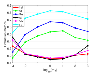
Refer to caption
(a) RBRL
Refer to caption
(b) Rank-SVM
Figure 4: Sensitivity analysis to the RBF hyper-parameter γ𝛾\gamma of RBRL and Rank-SVM on the image dataset. (m𝑚m is the feature size of the dataset.)

To conduct sensitivity analysis to the hyper-parameters {λ1,λ2,λ3}subscript𝜆1subscript𝜆2subscript𝜆3\{\lambda_{1},\lambda_{2},\lambda_{3}\} of RBRL, we evaluate the linear RBRL on the arts dataset. We first obtain the best hyper-parameters via fivefold cross-validation on the training set and then evaluate the performance effect of the other two with one hyper-parameter fixed. Figure 5 shows the results of the sensitivity analysis in terms of each evaluation metric. From Figure 5, it can be observed that RBRL is sensitive to the hyper-parameters. Besides, the best performance is obtained at some intermediate values of λ1subscript𝜆1\lambda_{1}, λ2subscript𝜆2\lambda_{2}, and λ3subscript𝜆3\lambda_{3}. Moreover, with the change of hyper-parameters, there are similar variations for all the evaluation metrics, especially ranking-based metrics (i.e., Ranking Loss, Coverage and Average Precision).
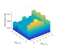
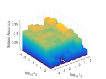
Refer to caption
Refer to caption
Refer to caption
Refer to caption
Refer to caption
Refer to caption
Refer to caption
Refer to caption
Refer to caption
Refer to caption
Refer to caption
Refer to caption
Refer to caption
Refer to caption
Refer to caption
Refer to caption
Refer to caption
Refer to caption
Figure 5: Sensitivity analysis to the hyper-parameters of the linear RBRL on the arts dataset. (a)-(f) The sensitivity of each evaluation metric with λ1subscript𝜆1\lambda_{1} fixed. (g)-(l) The sensitivity of each evaluation metric with λ2subscript𝜆2\lambda_{2} fixed. (m)-(r) The sensitivity of each evaluation metric with λ3subscript𝜆3\lambda_{3} fixed.

5.3.5 Computational Time Cost

We compare the one partition computational time cost for all the comparing methods on all the datasets. All the experiments are conducted on a laptop machine with 4×\times2.5GHz CPUs and 8GB RAM. Table 7 reports the average CPU time to train and test various methods. Generally, C++ or Java runs faster than Matlab, thus it’s unfair to compare methods with different language implementations. Compared with two recent methods (i.e., CPNL and MLFE), RBRL achieves a comparable time cost. For the last six datasets (corresponding to the linear model), RBRL is more efficient than Rank-SVM because our linear RBRL implementation can be viewed as an acceleration of kernel RBRL with linear kernel while Rank-SVM implementation doesn’t employ this linear acceleration. Besides, in the first four datasets (corresponding to the RBF kernel model), RBRL is slower than Rank-SVM, and better algorithms can be considered to improve the training efficiency of RBRL.

Table 7: The computational time cost (in seconds) for the various compared methods. The second row shows the programming language used to implement the corresponding methods. (“tr” indicates the training time cost. “te” indicates the test time cost.)
Rank-SVM Rank-SVMz BR ML-kNN CLR RAKEL CPNL MLFE RBRL
Matlab C++ Java Java Java Java Matlab Matlab Matlab
tr te tr te tr te tr te tr te tr te tr te tr te tr te
emotions 27 0.2 9 0.1 1 0.5 0.2 0.1 2 1 3 1 38 0.2 13 0.2 199 0.2
image 60 4 47 2 21 7 5 3 30 14 70 16 3919 11 1174 1 2118 11
scene 102 7 91 3 22 7 6 4 32 19 86 23 6433 15 2253 0.4 3525 16
yeast 1584 5 402 2 31 15 3 2 70 49 64 14 2480 4 353 0.8 5158 5
enron 12217 12 2394 5 7 3 2 1 38 28 26 1 713 0 1883 2 9998 0
arts 7794 35 5153 13 75 1 37 24 144 7 1103 2 280 0 1717 4 1495 0
education 11390 57 7663 18 78 1 53 35 130 12 1294 2 285 0 1960 5 1788 0
recreation 4733 58 3700 10 59 1 46 31 145 8 1348 2 168 0 1794 4 1252 0
science 16435 80 11271 27 107 2 76 51 182 25 2467 2 398 0 2434 5 2759 0
business 3109 30 3650 15 53 1 47 30 136 9 621 1 295 0 1588 4 1585 0

6 Conclusions

In this paper, we have presented a novel multi-label classification model, which joints Rank-SVM and Binary Relevance with robust Low-rank learning (RBRL). It incorporates the thresholding step into the ranking learning step of Rank-SVM via BR to train the model in only one step. Besides, the low-rank constraint is utilized to further exploit the label correlations. In addition, the kernelization RBRL is presented to obtain nonlinear multi-label classifiers. Moreover, two accelerated proximal gradient methods (APG) are employed to solve the linear and kernel RBRL efficiently. Extensive experiments against several state-of-the-art approaches have confirmed the effectiveness of our approach RBRL.

In the future, it’s interesting to combine the linear RBRL with deep neural networks (such as CNN) to learn from the raw multi-label data.

Acknowledgements

This work has been partially supported by grants from: Science and Technology Service Network Program of Chinese Academy of Sciences (STS Program, No. KFJ-STS-ZDTP-060), and National Natural Science Foundation of China (No. 71731009, 61472390, 71331005, 91546201).

Conflict of interest

Declarations of interest: none.

Appendix A Proof of Theorem 1

Proof.  The problem (9) can be rewritten as

min𝐖12i=1nj=1lmax(0,1yij𝐰j,ϕ(𝐱i))2+λ12𝐖F2+λ22i=1n1|Yi+||Yi|pYi+qYimax(0,2𝐰p𝐰q,ϕ(𝐱i))2s.t.Rank(𝐖)kformulae-sequencesubscript𝐖12superscriptsubscript𝑖1𝑛superscriptsubscript𝑗1𝑙𝑚𝑎𝑥superscript01subscript𝑦𝑖𝑗superscript𝐰𝑗italic-ϕsubscript𝐱𝑖2subscript𝜆12superscriptsubscriptdelimited-∥∥𝐖𝐹2subscript𝜆22superscriptsubscript𝑖1𝑛1superscriptsubscript𝑌𝑖superscriptsubscript𝑌𝑖subscript𝑝superscriptsubscript𝑌𝑖subscript𝑞superscriptsubscript𝑌𝑖𝑚𝑎𝑥superscript02superscript𝐰𝑝superscript𝐰𝑞italic-ϕsubscript𝐱𝑖2𝑠𝑡𝑅𝑎𝑛𝑘𝐖𝑘\begin{split}&\min\limits_{\mathbf{W}}\ \frac{1}{2}\sum_{i=1}^{n}\sum_{j=1}^{l}max(0,1-y_{ij}\langle\mathbf{w}^{j},\phi(\mathbf{x}_{i})\rangle)^{2}+\frac{\lambda_{1}}{2}\|\mathbf{W}\|_{F}^{2}+\\ &\qquad\frac{\lambda_{2}}{2}\sum_{i=1}^{n}\frac{1}{|Y_{i}^{+}||Y_{i}^{-}|}\sum_{p\in Y_{i}^{+}}\sum_{q\in Y_{i}^{-}}max(0,2-\langle\mathbf{w}^{p}-\mathbf{w}^{q},\phi(\mathbf{x}_{i})\rangle)^{2}\\ &s.t.\ Rank(\mathbf{W})\leq k\end{split} (40)

Denote the objective function in (40) except the second term as f(𝐖,Φ(𝐗),𝐘)𝑓𝐖Φ𝐗𝐘f(\mathbf{W},\Phi(\mathbf{X}),\mathbf{Y}). Hence, the optimization problem becomes minRank(𝐖)kf(𝐖,Φ(𝐗),𝐘)+λ12𝐖F2subscript𝑅𝑎𝑛𝑘𝐖𝑘𝑓𝐖Φ𝐗𝐘subscript𝜆12superscriptsubscriptnorm𝐖𝐹2\min\limits_{Rank(\mathbf{W})\leq k}f(\mathbf{W},\Phi(\mathbf{X}),\mathbf{Y})+\frac{\lambda_{1}}{2}\|\mathbf{W}\|_{F}^{2}.

Let 𝐖=[𝐰1,𝐰2,,𝐰l]subscript𝐖superscriptsubscript𝐰1superscriptsubscript𝐰2superscriptsubscript𝐰𝑙\mathbf{W}_{*}=[\mathbf{w}_{*}^{1},\mathbf{w}_{*}^{2},...,\mathbf{w}_{*}^{l}] be an optimal solution of (40). Because 𝐰jsuperscriptsubscript𝐰𝑗\mathbf{w}_{*}^{j} is an element of a Hilbert space for all j𝑗j, we can rewrite 𝐖subscript𝐖\mathbf{W}_{*} as

𝐰j=i=1nαijϕ(𝐱i)+𝐮j=Φ(𝐗)αj+𝐮j,j=1,,lformulae-sequencesuperscriptsubscript𝐰𝑗superscriptsubscript𝑖1𝑛subscript𝛼𝑖𝑗italic-ϕsubscript𝐱𝑖superscript𝐮𝑗Φsuperscript𝐗topsuperscript𝛼𝑗superscript𝐮𝑗𝑗1𝑙\mathbf{w}_{*}^{j}=\sum_{i=1}^{n}\alpha_{ij}\phi(\mathbf{x}_{i})+\mathbf{u}^{j}=\Phi(\mathbf{X})^{\top}\alpha^{j}+\mathbf{u}^{j},\ j=1,...,l (41)

or equivalently

𝐖=Φ(𝐗)𝐀+𝐔subscript𝐖Φsuperscript𝐗top𝐀𝐔\mathbf{W}_{*}=\Phi(\mathbf{X})^{\top}\mathbf{A}+\mathbf{U} (42)

where 𝐔=[𝐮1,𝐮2,,𝐮l]𝐔superscript𝐮1superscript𝐮2superscript𝐮𝑙\mathbf{U}=[\mathbf{u}^{1},\mathbf{u}^{2},...,\mathbf{u}^{l}], 𝐀=[α1,,αl]𝐀subscript𝛼1subscript𝛼𝑙\mathbf{A}=[\alpha_{1},...,\alpha_{l}] and 𝐮j,ϕ(𝐱i)=0superscript𝐮𝑗italic-ϕsubscript𝐱𝑖0\langle\mathbf{u}^{j},\phi(\mathbf{x}_{i})\rangle=0 for all i,j𝑖𝑗i,j. Set 𝐖=𝐖𝐔𝐖subscript𝐖𝐔\mathbf{W}=\mathbf{W}_{*}-\mathbf{U}. Clearly, 𝐖F2=𝐖F2+𝐔F2superscriptsubscriptnormsubscript𝐖𝐹2superscriptsubscriptnorm𝐖𝐹2superscriptsubscriptnorm𝐔𝐹2\|\mathbf{W}_{*}\|_{F}^{2}=\|\mathbf{W}\|_{F}^{2}+\|\mathbf{U}\|_{F}^{2}, and λ1>0subscript𝜆10\lambda_{1}>0, thus λ12𝐖F2λ12𝐖F2subscript𝜆12superscriptsubscriptnorm𝐖𝐹2subscript𝜆12superscriptsubscriptnormsubscript𝐖𝐹2\frac{\lambda_{1}}{2}\|\mathbf{W}\|_{F}^{2}\leq\frac{\lambda_{1}}{2}\|\mathbf{W}_{*}\|_{F}^{2}. Assume that there exsits 𝐀𝐀\mathbf{A} such that Rank(𝐀)k𝑅𝑎𝑛𝑘𝐀𝑘Rank(\mathbf{A})\leq k, thus Rank(𝐖)k𝑅𝑎𝑛𝑘𝐖𝑘Rank(\mathbf{W})\leq k. Additionally, for all i,j𝑖𝑗i,j we have that

𝐰j,ϕ(𝐱i)=𝐰j𝐮j,ϕ(𝐱i)=𝐰j,ϕ(𝐱i)superscript𝐰𝑗italic-ϕsubscript𝐱𝑖superscriptsubscript𝐰𝑗superscript𝐮𝑗italic-ϕsubscript𝐱𝑖superscriptsubscript𝐰𝑗italic-ϕsubscript𝐱𝑖\langle\mathbf{w}^{j},\phi(\mathbf{x}_{i})\rangle=\langle\mathbf{w}_{*}^{j}-\mathbf{u}^{j},\phi(\mathbf{x}_{i})\rangle=\langle\mathbf{w}_{*}^{j},\phi(\mathbf{x}_{i})\rangle (43)

hence

f(𝐖,Φ(𝐗),𝐘)=f(𝐖,Φ(𝐗),𝐘)𝑓𝐖Φ𝐗𝐘𝑓subscript𝐖Φ𝐗𝐘f(\mathbf{W},\Phi(\mathbf{X}),\mathbf{Y})=f(\mathbf{W}_{*},\Phi(\mathbf{X}),\mathbf{Y}) (44)

It can be observed that the objective function of (40) at 𝐖𝐖\mathbf{W} cannot be larger than the objective function at 𝐖subscript𝐖\mathbf{W}_{*}. Besides, 𝐖𝐖\mathbf{W} is also in the feasible region (i.e., Rank(𝐖)k𝑅𝑎𝑛𝑘𝐖𝑘Rank(\mathbf{W})\leq k). Thus, 𝐖=Φ(𝐗)𝐀,s.t.Rank(𝐀)kformulae-sequence𝐖Φsuperscript𝐗top𝐀𝑠𝑡𝑅𝑎𝑛𝑘𝐀𝑘\mathbf{W}=\Phi(\mathbf{X})^{\top}\mathbf{A},\ s.t.\ Rank(\mathbf{A})\leq k is also an optimal solution. \square

Appendix B Proof of Theorem 2

B.1 Proof of the Lemma 2

Proof.ai,ajmfor-allsubscript𝑎𝑖subscript𝑎𝑗superscript𝑚\forall\ a_{i},a_{j}\in\mathbb{R}^{m}, it always holds

2ai,ajai2+aj22subscript𝑎𝑖subscript𝑎𝑗superscriptnormsubscript𝑎𝑖2superscriptnormsubscript𝑎𝑗22\langle a_{i},a_{j}\rangle\leq\|a_{i}\|^{2}+\|a_{j}\|^{2} (45)

Thus, a1,a2,,anmfor-allsubscript𝑎1subscript𝑎2subscript𝑎𝑛superscript𝑚\forall\ a_{1},a_{2},...,a_{n}\in\mathbb{R}^{m}, we have

a1+a2++an2=i=1nai2+iji2ai,aji=1nai2+iji(ai2+aj2)=ni=1nai2superscriptdelimited-∥∥subscript𝑎1subscript𝑎2subscript𝑎𝑛2superscriptsubscript𝑖1𝑛superscriptdelimited-∥∥subscript𝑎𝑖2subscript𝑖subscript𝑗𝑖2subscript𝑎𝑖subscript𝑎𝑗superscriptsubscript𝑖1𝑛superscriptdelimited-∥∥subscript𝑎𝑖2subscript𝑖subscript𝑗𝑖superscriptdelimited-∥∥subscript𝑎𝑖2superscriptdelimited-∥∥subscript𝑎𝑗2𝑛superscriptsubscript𝑖1𝑛superscriptdelimited-∥∥subscript𝑎𝑖2\begin{split}&\|a_{1}+a_{2}+...+a_{n}\|^{2}\\ &=\sum_{i=1}^{n}\|a_{i}\|^{2}+\sum_{i}\sum_{j\neq i}2\langle a_{i},a_{j}\rangle\\ &\leq\sum_{i=1}^{n}\|a_{i}\|^{2}+\sum_{i}\sum_{j\neq i}(\|a_{i}\|^{2}+\|a_{j}\|^{2})\\ &=n\sum_{i=1}^{n}\|a_{i}\|^{2}\end{split} (46)

\square

B.2 Proof of the Proposition 1

Proof.  Firstly, we compute the Lipschitz constant for fr𝐰j,j=1,2,,lformulae-sequencesubscript𝑓𝑟superscript𝐰𝑗𝑗12𝑙\frac{\partial f_{r}}{\partial{\mathbf{w}^{j}}},j=1,2,...,l. 𝐮1,𝐮2mfor-allsubscript𝐮1subscript𝐮2superscript𝑚\forall\ \mathbf{u}_{1},\mathbf{u}_{2}\in\mathbb{R}^{m}, we have

fr(𝐮1)𝐰jfr(𝐮2)𝐰j2=i=1n1|Yi+||Yi|{[[jYi+]]qYi(|2𝐮1𝐰q,𝐱i|+|2𝐮2𝐰q,𝐱i|+)(𝐱i)+[[jYi]]pYi+(|2𝐰p𝐮1,𝐱i|+|2𝐰p𝐮2,𝐱i|+)𝐱i}2{i=1n([[jYi+]]|Yi|+[[jYi]]|Yi+|)}i=1n1|Yi+|2|Yi|2{[[jYi+]]qYi(|2𝐮1𝐰q,𝐱i|+|2𝐮2𝐰q,𝐱i|+)(𝐱i)2+[[jYi]]pYi+(|2𝐰p𝐮1,𝐱i|+|2𝐰p𝐮2,𝐱i|+)𝐱i2}{i=1n([[jYi+]]|Yi|+[[jYi]]|Yi+|)}i=1n1|Yi+|2|Yi|2{[[jYi+]]qYi𝐮2𝐮1,𝐱i2+[[jYi]]pYi+𝐮1𝐮2,𝐱i2}𝐱i2{i=1n([[jYi+]]|Yi|+[[jYi]]|Yi+|)}i=1n[[jYi+]]|Yi|+[[jYi]]|Yi+||Yi+|2|Yi|2𝐱i2𝐱i2𝐮1𝐮22={i=1n([[jYi+]]|Yi|+[[jYi]]|Yi+|)}{i=1n([[jYi+]]|Yi|+[[jYi]]|Yi+|)𝐱i4|Yi+|2|Yi|2}Δ𝐮2superscriptdelimited-∥∥subscript𝑓𝑟subscript𝐮1superscript𝐰𝑗subscript𝑓𝑟subscript𝐮2superscript𝐰𝑗2superscriptdelimited-∥∥superscriptsubscript𝑖1𝑛1superscriptsubscript𝑌𝑖superscriptsubscript𝑌𝑖delimited-[]delimited-[]𝑗superscriptsubscript𝑌𝑖subscript𝑞superscriptsubscript𝑌𝑖subscript2subscript𝐮1superscript𝐰𝑞subscript𝐱𝑖subscript2subscript𝐮2superscript𝐰𝑞subscript𝐱𝑖subscript𝐱𝑖delimited-[]delimited-[]𝑗superscriptsubscript𝑌𝑖subscript𝑝superscriptsubscript𝑌𝑖subscript2superscript𝐰𝑝subscript𝐮1subscript𝐱𝑖subscript2superscript𝐰𝑝subscript𝐮2subscript𝐱𝑖subscript𝐱𝑖2superscriptsubscript𝑖1𝑛delimited-[]delimited-[]𝑗superscriptsubscript𝑌𝑖superscriptsubscript𝑌𝑖delimited-[]delimited-[]𝑗superscriptsubscript𝑌𝑖superscriptsubscript𝑌𝑖superscriptsubscript𝑖1𝑛1superscriptsuperscriptsubscript𝑌𝑖2superscriptsuperscriptsubscript𝑌𝑖2delimited-[]delimited-[]𝑗superscriptsubscript𝑌𝑖subscript𝑞superscriptsubscript𝑌𝑖superscriptdelimited-∥∥subscript2subscript𝐮1superscript𝐰𝑞subscript𝐱𝑖subscript2subscript𝐮2superscript𝐰𝑞subscript𝐱𝑖subscript𝐱𝑖2delimited-[]delimited-[]𝑗superscriptsubscript𝑌𝑖subscript𝑝superscriptsubscript𝑌𝑖superscriptdelimited-∥∥subscript2superscript𝐰𝑝subscript𝐮1subscript𝐱𝑖subscript2superscript𝐰𝑝subscript𝐮2subscript𝐱𝑖subscript𝐱𝑖2superscriptsubscript𝑖1𝑛delimited-[]delimited-[]𝑗superscriptsubscript𝑌𝑖superscriptsubscript𝑌𝑖delimited-[]delimited-[]𝑗superscriptsubscript𝑌𝑖superscriptsubscript𝑌𝑖superscriptsubscript𝑖1𝑛1superscriptsuperscriptsubscript𝑌𝑖2superscriptsuperscriptsubscript𝑌𝑖2delimited-[]delimited-[]𝑗superscriptsubscript𝑌𝑖subscript𝑞superscriptsubscript𝑌𝑖superscriptdelimited-∥∥subscript𝐮2subscript𝐮1subscript𝐱𝑖2delimited-[]delimited-[]𝑗superscriptsubscript𝑌𝑖subscript𝑝superscriptsubscript𝑌𝑖superscriptdelimited-∥∥subscript𝐮1subscript𝐮2subscript𝐱𝑖2superscriptdelimited-∥∥subscript𝐱𝑖2superscriptsubscript𝑖1𝑛delimited-[]delimited-[]𝑗superscriptsubscript𝑌𝑖superscriptsubscript𝑌𝑖delimited-[]delimited-[]𝑗superscriptsubscript𝑌𝑖superscriptsubscript𝑌𝑖superscriptsubscript𝑖1𝑛delimited-[]delimited-[]𝑗superscriptsubscript𝑌𝑖superscriptsubscript𝑌𝑖delimited-[]delimited-[]𝑗superscriptsubscript𝑌𝑖superscriptsubscript𝑌𝑖superscriptsuperscriptsubscript𝑌𝑖2superscriptsuperscriptsubscript𝑌𝑖2superscriptdelimited-∥∥subscript𝐱𝑖2superscriptdelimited-∥∥subscript𝐱𝑖2superscriptdelimited-∥∥subscript𝐮1subscript𝐮22superscriptsubscript𝑖1𝑛delimited-[]delimited-[]𝑗superscriptsubscript𝑌𝑖superscriptsubscript𝑌𝑖delimited-[]delimited-[]𝑗superscriptsubscript𝑌𝑖superscriptsubscript𝑌𝑖superscriptsubscript𝑖1𝑛delimited-[]delimited-[]𝑗superscriptsubscript𝑌𝑖superscriptsubscript𝑌𝑖delimited-[]delimited-[]𝑗superscriptsubscript𝑌𝑖superscriptsubscript𝑌𝑖superscriptnormsubscript𝐱𝑖4superscriptsuperscriptsubscript𝑌𝑖2superscriptsuperscriptsubscript𝑌𝑖2superscriptdelimited-∥∥Δ𝐮2\begin{split}&\|\frac{\partial f_{r}(\mathbf{u}_{1})}{\partial{\mathbf{w}^{j}}}-\frac{\partial f_{r}(\mathbf{u}_{2})}{\partial{\mathbf{w}^{j}}}\|^{2}\\ &=\|\sum_{i=1}^{n}\frac{1}{|Y_{i}^{+}||Y_{i}^{-}|}\Big{\{}[\![j\in Y_{i}^{+}]\!]\sum_{q\in Y_{i}^{-}}(|2-\langle\mathbf{u}_{1}-\mathbf{w}^{q},\mathbf{x}_{i}\rangle|_{+}-|2-\langle\mathbf{u}_{2}-\mathbf{w}^{q},\mathbf{x}_{i}\rangle|_{+})(-\mathbf{x}_{i})\\ &\quad+[\![j\in Y_{i}^{-}]\!]\sum_{p\in Y_{i}^{+}}(|2-\langle\mathbf{w}^{p}-\mathbf{u}_{1},\mathbf{x}_{i}\rangle|_{+}-|2-\langle\mathbf{w}^{p}-\mathbf{u}_{2},\mathbf{x}_{i}\rangle|_{+})\mathbf{x}_{i}\Big{\}}\|^{2}\\ &\leq\Big{\{}\sum_{i=1}^{n}([\![j\in Y_{i}^{+}]\!]|Y_{i}^{-}|+[\![j\in Y_{i}^{-}]\!]|Y_{i}^{+}|)\Big{\}}\sum_{i=1}^{n}\frac{1}{|Y_{i}^{+}|^{2}|Y_{i}^{-}|^{2}}\Big{\{}[\![j\in Y_{i}^{+}]\!]\sum_{q\in Y_{i}^{-}}\|(|2-\langle\mathbf{u}_{1}-\mathbf{w}^{q},\mathbf{x}_{i}\rangle|_{+}\\ &\quad-|2-\langle\mathbf{u}_{2}-\mathbf{w}^{q},\mathbf{x}_{i}\rangle|_{+})(-\mathbf{x}_{i})\|^{2}+[\![j\in Y_{i}^{-}]\!]\sum_{p\in Y_{i}^{+}}\|(|2-\langle\mathbf{w}^{p}-\mathbf{u}_{1},\mathbf{x}_{i}\rangle|_{+}\\ &\quad-|2-\langle\mathbf{w}^{p}-\mathbf{u}_{2},\mathbf{x}_{i}\rangle|_{+})\mathbf{x}_{i}\|^{2}\Big{\}}\\ &\leq\Big{\{}\sum_{i=1}^{n}([\![j\in Y_{i}^{+}]\!]|Y_{i}^{-}|+[\![j\in Y_{i}^{-}]\!]|Y_{i}^{+}|)\Big{\}}\sum_{i=1}^{n}\frac{1}{|Y_{i}^{+}|^{2}|Y_{i}^{-}|^{2}}\Big{\{}[\![j\in Y_{i}^{+}]\!]\sum_{q\in Y_{i}^{-}}\|\langle\mathbf{u}_{2}-\mathbf{u}_{1},\mathbf{x}_{i}\rangle\|^{2}\\ &\quad+[\![j\in Y_{i}^{-}]\!]\sum_{p\in Y_{i}^{+}}\|\langle\mathbf{u}_{1}-\mathbf{u}_{2},\mathbf{x}_{i}\rangle\|^{2}\Big{\}}\|\mathbf{x}_{i}\|^{2}\\ &\leq\Big{\{}\sum_{i=1}^{n}([\![j\in Y_{i}^{+}]\!]|Y_{i}^{-}|+[\![j\in Y_{i}^{-}]\!]|Y_{i}^{+}|)\Big{\}}\sum_{i=1}^{n}\frac{[\![j\in Y_{i}^{+}]\!]|Y_{i}^{-}|+[\![j\in Y_{i}^{-}]\!]|Y_{i}^{+}|}{|Y_{i}^{+}|^{2}|Y_{i}^{-}|^{2}}\|\mathbf{x}_{i}\|^{2}\|\mathbf{x}_{i}\|^{2}\|\mathbf{u}_{1}-\mathbf{u}_{2}\|^{2}\\ &=\Big{\{}\sum_{i=1}^{n}([\![j\in Y_{i}^{+}]\!]|Y_{i}^{-}|+[\![j\in Y_{i}^{-}]\!]|Y_{i}^{+}|)\Big{\}}\Big{\{}\sum_{i=1}^{n}\frac{([\![j\in Y_{i}^{+}]\!]|Y_{i}^{-}|+[\![j\in Y_{i}^{-}]\!]|Y_{i}^{+}|)\|\mathbf{x}_{i}\|^{4}}{|Y_{i}^{+}|^{2}|Y_{i}^{-}|^{2}}\Big{\}}\|\Delta\mathbf{u}\|^{2}\end{split} (47)

where Δ𝐮=𝐮1𝐮2Δ𝐮subscript𝐮1subscript𝐮2\Delta\mathbf{u}=\mathbf{u}_{1}-\mathbf{u}_{2}. Thus, the Lipschitz constant for fr𝐰j,j=1,2,,lformulae-sequencesubscript𝑓𝑟superscript𝐰𝑗𝑗12𝑙\frac{\partial f_{r}}{\partial{\mathbf{w}^{j}}},j=1,2,...,l is as follows.

Lfrj=AjBjsuperscriptsubscript𝐿subscript𝑓𝑟𝑗subscript𝐴𝑗subscript𝐵𝑗L_{f_{r}}^{j}=\sqrt{A_{j}*B_{j}} (48)

where Bj=i=1n([[jYi+]]|Yi|+[[jYi]]|Yi+|)𝐱i4|Yi+|2|Yi|2subscript𝐵𝑗superscriptsubscript𝑖1𝑛delimited-[]delimited-[]𝑗superscriptsubscript𝑌𝑖superscriptsubscript𝑌𝑖delimited-[]delimited-[]𝑗superscriptsubscript𝑌𝑖superscriptsubscript𝑌𝑖superscriptnormsubscript𝐱𝑖4superscriptsuperscriptsubscript𝑌𝑖2superscriptsuperscriptsubscript𝑌𝑖2B_{j}=\sum_{i=1}^{n}\frac{([\![j\in Y_{i}^{+}]\!]|Y_{i}^{-}|+[\![j\in Y_{i}^{-}]\!]|Y_{i}^{+}|)\|\mathbf{x}_{i}\|^{4}}{|Y_{i}^{+}|^{2}|Y_{i}^{-}|^{2}}, and Aj=i=1n([[jYi+]]|Yi|+[[jYi]]|Yi+|),j=1,,lformulae-sequencesubscript𝐴𝑗superscriptsubscript𝑖1𝑛delimited-[]delimited-[]𝑗superscriptsubscript𝑌𝑖superscriptsubscript𝑌𝑖delimited-[]delimited-[]𝑗superscriptsubscript𝑌𝑖superscriptsubscript𝑌𝑖𝑗1𝑙A_{j}=\sum_{i=1}^{n}([\![j\in Y_{i}^{+}]\!]|Y_{i}^{-}|+[\![j\in Y_{i}^{-}]\!]|Y_{i}^{+}|),j=1,...,l.

Then, for 𝐖fr(𝐖)=[fr𝐰1,fr𝐰2,,fr𝐰l]subscript𝐖subscript𝑓𝑟𝐖subscript𝑓𝑟superscript𝐰1subscript𝑓𝑟superscript𝐰2subscript𝑓𝑟superscript𝐰𝑙\nabla_{\mathbf{W}}{f_{r}(\mathbf{W})}=[\frac{\partial f_{r}}{\partial{\mathbf{w}^{1}}},\frac{\partial f_{r}}{\partial{\mathbf{w}^{2}}},...,\frac{\partial f_{r}}{\partial{\mathbf{w}^{l}}}], 𝐔1,𝐔2m×lfor-allsubscript𝐔1subscript𝐔2superscript𝑚𝑙\forall\ \mathbf{U}_{1},\mathbf{U}_{2}\in\mathbb{R}^{m\times l}, we have

fr(𝐔1)fr(𝐔2)F2=j=1lfr(𝐮1j)𝐰jfr(𝐮2j)𝐰j2i=1l(Lfj)2Δ𝐮j2=i=1lAjBjΔ𝐮j2max{AjBj}j=1,,l(i=1lΔ𝐮j2)=max{AjBj}j=1,,lΔ𝐔F2superscriptsubscriptdelimited-∥∥subscript𝑓𝑟subscript𝐔1subscript𝑓𝑟subscript𝐔2𝐹2superscriptsubscript𝑗1𝑙superscriptdelimited-∥∥subscript𝑓𝑟superscriptsubscript𝐮1𝑗superscript𝐰𝑗subscript𝑓𝑟superscriptsubscript𝐮2𝑗superscript𝐰𝑗2superscriptsubscript𝑖1𝑙superscriptsuperscriptsubscript𝐿𝑓𝑗2superscriptdelimited-∥∥Δsuperscript𝐮𝑗2superscriptsubscript𝑖1𝑙subscript𝐴𝑗subscript𝐵𝑗superscriptdelimited-∥∥Δsuperscript𝐮𝑗2𝑚𝑎𝑥subscriptsubscript𝐴𝑗subscript𝐵𝑗𝑗1𝑙superscriptsubscript𝑖1𝑙superscriptdelimited-∥∥Δsuperscript𝐮𝑗2𝑚𝑎𝑥subscriptsubscript𝐴𝑗subscript𝐵𝑗𝑗1𝑙superscriptsubscriptdelimited-∥∥Δ𝐔𝐹2\begin{split}&\|\nabla{f_{r}(\mathbf{U}_{1})}-\nabla{f_{r}(\mathbf{U}_{2})}\|_{F}^{2}\\ &=\sum_{j=1}^{l}\|\frac{\partial f_{r}(\mathbf{u}_{1}^{j})}{\partial{\mathbf{w}^{j}}}-\frac{\partial f_{r}(\mathbf{u}_{2}^{j})}{\partial{\mathbf{w}^{j}}}\|^{2}\\ &\leq\sum_{i=1}^{l}(L_{f}^{j})^{2}\|\Delta\mathbf{u}^{j}\|^{2}\\ &=\sum_{i=1}^{l}A_{j}B_{j}\|\Delta\mathbf{u}^{j}\|^{2}\\ &\leq max\{A_{j}B_{j}\}_{j=1,...,l}(\sum_{i=1}^{l}\|\Delta\mathbf{u}^{j}\|^{2})\\ &=max\{A_{j}B_{j}\}_{j=1,...,l}\|\Delta\mathbf{U}\|_{F}^{2}\end{split} (49)

where Δ𝐔=𝐔1𝐔2Δ𝐔subscript𝐔1subscript𝐔2\Delta\mathbf{U}=\mathbf{U}_{1}-\mathbf{U}_{2}, l𝑙l is the number of the labels, Bj=i=1n([[jYi+]]|Yi|+[[jYi]]|Yi+|)𝐱i4|Yi+|2|Yi|2subscript𝐵𝑗superscriptsubscript𝑖1𝑛delimited-[]delimited-[]𝑗superscriptsubscript𝑌𝑖superscriptsubscript𝑌𝑖delimited-[]delimited-[]𝑗superscriptsubscript𝑌𝑖superscriptsubscript𝑌𝑖superscriptnormsubscript𝐱𝑖4superscriptsuperscriptsubscript𝑌𝑖2superscriptsuperscriptsubscript𝑌𝑖2B_{j}=\sum_{i=1}^{n}\frac{([\![j\in Y_{i}^{+}]\!]|Y_{i}^{-}|+[\![j\in Y_{i}^{-}]\!]|Y_{i}^{+}|)\|\mathbf{x}_{i}\|^{4}}{|Y_{i}^{+}|^{2}|Y_{i}^{-}|^{2}}, and Aj=i=1n([[jYi+]]|Yi|+[[jYi]]|Yi+|),j=1,,lformulae-sequencesubscript𝐴𝑗superscriptsubscript𝑖1𝑛delimited-[]delimited-[]𝑗superscriptsubscript𝑌𝑖superscriptsubscript𝑌𝑖delimited-[]delimited-[]𝑗superscriptsubscript𝑌𝑖superscriptsubscript𝑌𝑖𝑗1𝑙A_{j}=\sum_{i=1}^{n}([\![j\in Y_{i}^{+}]\!]|Y_{i}^{-}|+[\![j\in Y_{i}^{-}]\!]|Y_{i}^{+}|),j=1,...,l. \square

B.3 Proof of the Theorem 2

Proof.𝐖1,𝐖2m×lfor-allsubscript𝐖1subscript𝐖2superscript𝑚𝑙\forall\ \mathbf{W}_{1},\mathbf{W}_{2}\in\mathbb{R}^{m\times l}, we have

f(𝐖1)f(𝐖2)F2=𝐗((|𝐄𝐘(𝐗𝐖1)|+|𝐄𝐘(𝐗𝐖2)|+)(𝐘))+λ1Δ𝐖+λ2(fr(𝐖1)fr(𝐖2))F23𝐗((|𝐄𝐘(𝐗𝐖1)|+|𝐄𝐘(𝐗𝐖2)|+)(𝐘))F2+3λ1Δ𝐖F2+3λ2(fr(𝐖1)fr(𝐖2))F23𝐗F2|𝐄𝐘(𝐗𝐖1)|+|𝐄𝐘(𝐗𝐖2)|+F2+3λ12Δ𝐖F2+3(λ2Lfr)2Δ𝐖F23𝐗F2𝐘(𝐗Δ𝐖)F2+3λ12Δ𝐖F2+3(λ2Lfr)2Δ𝐖F23𝐗F2𝐗F2Δ𝐖F2+3λ12Δ𝐖F2+3(λ2Lfr)2Δ𝐖F2=(3(𝐗F2)2+3λ12+3(λ2Lfr)2)Δ𝐖F2superscriptsubscriptdelimited-∥∥𝑓subscript𝐖1𝑓subscript𝐖2𝐹2superscriptsubscriptdelimited-∥∥superscript𝐗topsubscript𝐄𝐘subscript𝐗𝐖1subscript𝐄𝐘subscript𝐗𝐖2𝐘subscript𝜆1Δ𝐖subscript𝜆2subscript𝑓𝑟subscript𝐖1subscript𝑓𝑟subscript𝐖2𝐹23superscriptsubscriptdelimited-∥∥superscript𝐗topsubscript𝐄𝐘subscript𝐗𝐖1subscript𝐄𝐘subscript𝐗𝐖2𝐘𝐹23superscriptsubscriptdelimited-∥∥subscript𝜆1Δ𝐖𝐹23superscriptsubscriptdelimited-∥∥subscript𝜆2subscript𝑓𝑟subscript𝐖1subscript𝑓𝑟subscript𝐖2𝐹23superscriptsubscriptdelimited-∥∥superscript𝐗top𝐹2superscriptsubscriptdelimited-∥∥subscript𝐄𝐘subscript𝐗𝐖1subscript𝐄𝐘subscript𝐗𝐖2𝐹23superscriptsubscript𝜆12superscriptsubscriptdelimited-∥∥Δ𝐖𝐹23superscriptsubscript𝜆2subscript𝐿subscript𝑓𝑟2superscriptsubscriptdelimited-∥∥Δ𝐖𝐹23superscriptsubscriptdelimited-∥∥𝐗𝐹2superscriptsubscriptdelimited-∥∥𝐘𝐗Δ𝐖𝐹23superscriptsubscript𝜆12superscriptsubscriptdelimited-∥∥Δ𝐖𝐹23superscriptsubscript𝜆2subscript𝐿subscript𝑓𝑟2superscriptsubscriptdelimited-∥∥Δ𝐖𝐹23superscriptsubscriptdelimited-∥∥𝐗𝐹2superscriptsubscriptdelimited-∥∥𝐗𝐹2superscriptsubscriptdelimited-∥∥Δ𝐖𝐹23superscriptsubscript𝜆12superscriptsubscriptdelimited-∥∥Δ𝐖𝐹23superscriptsubscript𝜆2subscript𝐿subscript𝑓𝑟2superscriptsubscriptdelimited-∥∥Δ𝐖𝐹23superscriptsuperscriptsubscriptdelimited-∥∥𝐗𝐹223superscriptsubscript𝜆123superscriptsubscript𝜆2subscript𝐿subscript𝑓𝑟2superscriptsubscriptdelimited-∥∥Δ𝐖𝐹2\begin{split}&\|\nabla{f(\mathbf{W}_{1})}-\nabla{f(\mathbf{W}_{2})}\|_{F}^{2}\\ &=\|\mathbf{X}^{\top}((|\mathbf{E}-\mathbf{Y}\circ(\mathbf{XW}_{1})|_{+}-|\mathbf{E}-\mathbf{Y}\circ(\mathbf{XW}_{2})|_{+})\circ(-\mathbf{Y}))\\ &\quad+\lambda_{1}\Delta\mathbf{W}+\lambda_{2}(\nabla{f_{r}(\mathbf{W}_{1})}-\nabla{f_{r}(\mathbf{W}_{2})})\|_{F}^{2}\\ &\leq 3\|\mathbf{X}^{\top}((|\mathbf{E}-\mathbf{Y}\circ(\mathbf{XW}_{1})|_{+}-|\mathbf{E}-\mathbf{Y}\circ(\mathbf{XW}_{2})|_{+})\circ(-\mathbf{Y}))\|_{F}^{2}\\ &\quad+3\|\lambda_{1}\Delta\mathbf{W}\|_{F}^{2}+3\|\lambda_{2}(\nabla{f_{r}(\mathbf{W}_{1})}-\nabla{f_{r}(\mathbf{W}_{2})})\|_{F}^{2}\\ &\leq 3\|\mathbf{X}^{\top}\|_{F}^{2}\||\mathbf{E}-\mathbf{Y}\circ(\mathbf{XW}_{1})|_{+}-|\mathbf{E}-\mathbf{Y}\circ(\mathbf{XW}_{2})|_{+}\|_{F}^{2}\\ &\quad+3\lambda_{1}^{2}\|\Delta\mathbf{W}\|_{F}^{2}+3(\lambda_{2}L_{f_{r}})^{2}\|\Delta\mathbf{W}\|_{F}^{2}\\ &\leq 3\|\mathbf{X}\|_{F}^{2}\|-\mathbf{Y}\circ(\mathbf{X}\Delta\mathbf{W})\|_{F}^{2}+3\lambda_{1}^{2}\|\Delta\mathbf{W}\|_{F}^{2}+3(\lambda_{2}L_{f_{r}})^{2}\|\Delta\mathbf{W}\|_{F}^{2}\\ &\leq 3\|\mathbf{X}\|_{F}^{2}\|\mathbf{X}\|_{F}^{2}\|\Delta\mathbf{W}\|_{F}^{2}+3\lambda_{1}^{2}\|\Delta\mathbf{W}\|_{F}^{2}+3(\lambda_{2}L_{f_{r}})^{2}\|\Delta\mathbf{W}\|_{F}^{2}\\ &=(3(\|\mathbf{X}\|_{F}^{2})^{2}+3\lambda_{1}^{2}+3(\lambda_{2}L_{f_{r}})^{2})\|\Delta\mathbf{W}\|_{F}^{2}\end{split} (50)

where Δ𝐖=𝐖1𝐖2Δ𝐖subscript𝐖1subscript𝐖2\Delta\mathbf{W}=\mathbf{W}_{1}-\mathbf{W}_{2}. \square

References

References

  • Argyriou et al. [2008] Argyriou, A., Evgeniou, T., Pontil, M., 2008. Convex multi-task feature learning. Machine Learning 73 (3), 243–272.
  • Boutell et al. [2004] Boutell, M. R., Luo, J., Shen, X., Brown, C. M., 2004. Learning multi-label scene classification. Pattern Recognition 37 (9), 1757–1771.
  • Cai et al. [2010] Cai, J.-F., Candès, E. J., Shen, Z., 2010. A singular value thresholding algorithm for matrix completion. SIAM Journal on Optimization 20 (4), 1956–1982.
  • Chang and Lin [2011] Chang, C.-C., Lin, C.-J., 2011. LIBSVM: A library for support vector machines. ACM Transactions on Intelligent Systems and Technology 2, 27:1–27:27.
  • Clare and King [2001] Clare, A., King, R. D., 2001. Knowledge discovery in multi-label phenotype data. In: European Conference on Principles of Data Mining and Knowledge Discovery. Springer, pp. 42–53.
  • Cortes and Mohri [2004] Cortes, C., Mohri, M., 2004. Auc optimization vs. error rate minimization. In: Advances in Neural Information Processing Systems 16. pp. 313–320.
  • Demšar [2006] Demšar, J., 2006. Statistical comparisons of classifiers over multiple data sets. Journal of Machine Learning Research 7, 1–30.
  • Dinuzzo [2012] Dinuzzo, F., 2012. The representer theorem for hilbert spaces: a necessary and sufficient condition. In: Advances in Neural Information Processing Systems 25. pp. 189–196.
  • Elisseeff et al. [2001] Elisseeff, A., Weston, J., et al., 2001. A kernel method for multi-labelled classification. In: Advances in Neural Information Processing Systems 14. pp. 681–687.
  • Fan et al. [2008] Fan, R.-E., Chang, K.-W., Hsieh, C.-J., Wang, X.-R., Lin, C.-J., 2008. Liblinear: A library for large linear classification. Journal of Machine Learning Research 9, 1871–1874.
  • Frank and Wolfe [1956] Frank, M., Wolfe, P., 1956. An algorithm for quadratic programming. Naval Research Logistics Quarterly 3 (1-2), 95–110.
  • Friedman [1937] Friedman, M., 1937. The use of ranks to avoid the assumption of normality implicit in the analysis of variance. Journal of the American Statistical Association 32 (200), 675–701.
  • Fürnkranz et al. [2008] Fürnkranz, J., Hüllermeier, E., Loza Mencía, E., Brinker, K., 2008. Multilabel classification via calibrated label ranking. Machine Learning 73 (2), 133–153.
  • Ghamrawi and McCallum [2005] Ghamrawi, N., McCallum, A., 2005. Collective multi-label classification. In: Proceedings of the 14th ACM International Conference on Information and Knowledge Management. pp. 195–200.
  • Golub and Van Loan [1996] Golub, G. H., Van Loan, C. F., 1996. Matrix computations (3rd ed.). Johns Hopkins University, Press, Baltimore, MD, USA.
  • Gopal and Yang [2010] Gopal, S., Yang, Y., 2010. Multilabel classification with meta-level features. In: Proceedings of the 33rd international ACM SIGIR Conference on Research and Development in Information Retrieval. ACM, pp. 315–322.
  • Hou et al. [2016] Hou, P., Geng, X., Zhang, M.-L., 2016. Multi-label manifold learning. In: Proceedings of the 30th AAAI Conference on Artificial Intelligence. AAAI Press, pp. 1680–1686.
  • Hsu et al. [2003] Hsu, C.-W., Chang, C.-C., Lin, C.-J., et al., 2003. A practical guide to support vector classification.
  • Huang et al. [2015] Huang, J., Li, G., Huang, Q., Wu, X., 2015. Learning label specific features for multi-label classification. In: 2015 IEEE International Conference on Data Mining. pp. 181–190.
  • Huang et al. [2018] Huang, J., Li, G., Huang, Q., Wu, X., 2018. Joint feature selection and classification for multilabel learning. IEEE Transactions on Cybernetics 48 (3), 876–889.
  • Jaggi [2013] Jaggi, M., 2013. Revisiting frank-wolfe: Projection-free sparse convex optimization. In: Proceedings of the 30th International Conference on Machine Learning. pp. 427–435.
  • Ji and Ye [2009] Ji, S., Ye, J., 2009. An accelerated gradient method for trace norm minimization. In: Proceedings of the 26th International Conference on Machine Learning. pp. 457–464.
  • Jiang et al. [2008] Jiang, A., Wang, C., Zhu, Y., 2008. Calibrated rank-svm for multi-label image categorization. In: IEEE International Joint Conference on Neural Networks. pp. 1450–1455.
  • Jing et al. [2015] Jing, L., Yang, L., Yu, J., Ng, M. K., 2015. Semi-supervised low-rank mapping learning for multi-label classification. In: Proceedings of the IEEE Conference on Computer Vision and Pattern Recognition. pp. 1483–1491.
  • Kivinen et al. [2002] Kivinen, J., Smola, A., Williamson, R., 2002. Learning with kernels. MIT Press.
  • Li et al. [2012] Li, H., Chen, N., Li, L., 2012. Error analysis for matrix elastic-net regularization algorithms. IEEE Transactions on Neural Networks and Learning Systems 23 (5), 737–748.
  • McCallum [1999] McCallum, A., 1999. Multi-label text classification with a mixture model trained by em. In: AAAI’99 workshop on text learning. pp. 1–7.
  • Nesterov [2005] Nesterov, Y., 2005. Smooth minimization of non-smooth functions. Mathematical Programming 103 (1), 127–152.
  • Qi et al. [2007] Qi, G.-J., Hua, X.-S., Rui, Y., Tang, J., Mei, T., Zhang, H.-J., 2007. Correlative multi-label video annotation. In: Proceedings of the 15th International Conference on Multimedia. pp. 17–26.
  • Read et al. [2011] Read, J., Pfahringer, B., Holmes, G., Frank, E., 2011. Classifier chains for multi-label classification. Machine Learning 85 (3), 333–359.
  • Schapire and Singer [2000] Schapire, R. E., Singer, Y., 2000. Boostexter: A boosting-based system for text categorization. Machine Learning 39 (2-3), 135–168.
  • Schölkopf and Smola [2002] Schölkopf, B., Smola, A. J., 2002. Learning with kernels: support vector machines, regularization, optimization, and beyond. MIT Press.
  • Shalev-Shwartz and Ben-David [2014] Shalev-Shwartz, S., Ben-David, S., 2014. Understanding machine learning: From theory to algorithms. Cambridge University Press.
  • Trohidis et al. [2008] Trohidis, K., Tsoumakas, G., Kalliris, G., Vlahavas, I. P., 2008. Multi-label classification of music into emotions. In: ISMIR 2008, 9th International Conference on Music Information Retrieval. Vol. 8. pp. 325–330.
  • Tsoumakas and Katakis [2006] Tsoumakas, G., Katakis, I., 2006. Multi-label classification: An overview. International Journal of Data Warehousing and Mining 3 (3).
  • Tsoumakas et al. [2009] Tsoumakas, G., Katakis, I., Vlahavas, I., 2009. Mining multi-label data. In: Data mining and knowledge discovery handbook. Springer, pp. 667–685.
  • Tsoumakas et al. [2011a] Tsoumakas, G., Katakis, I., Vlahavas, I., 2011a. Random k-labelsets for multilabel classification. IEEE Transactions on Knowledge and Data Engineering 23 (7), 1079–1089.
  • Tsoumakas et al. [2011b] Tsoumakas, G., Spyromitros-Xioufis, E., Vilcek, J., Vlahavas, I., 2011b. Mulan: A java library for multi-label learning. Journal of Machine Learning Research 12, 2411–2414.
  • Ueda and Saito [2002] Ueda, N., Saito, K., 2002. Parametric mixture models for multi-labeled text. In: Advances in Neural Information Processing Systems 15. pp. 721–728.
  • Wang et al. [2009] Wang, H., Huang, H., Ding, C., 2009. Image annotation using multi-label correlated green’s function. In: IEEE 12th International Conference on Computer Vision. pp. 2029–2034.
  • Wang et al. [2016] Wang, J., Yang, Y., Mao, J., Huang, Z., Huang, C., Xu, W., 2016. Cnn-rnn: A unified framework for multi-label image classification. In: Proceedings of the IEEE Conference on Computer Vision and Pattern Recognition. pp. 2285–2294.
  • Wu et al. [2018a] Wu, G., Tian, Y., Liu, D., 2018a. Cost-sensitive multi-label learning with positive and negative label pairwise correlations. Neural Networks 108, 411–423.
  • Wu et al. [2018b] Wu, G., Tian, Y., Zhang, C., 2018b. A unified framework implementing linear binary relevance for multi-label learning. Neurocomputing 289, 86–100.
  • Wu et al. [2016] Wu, Q., Tan, M., Song, H., Chen, J., Ng, M. K., 2016. Ml-forest: A multi-label tree ensemble method for multi-label classification. IEEE Transactions on Knowledge and Data Engineering 28 (10), 2665–2680.
  • Wu and Zhou [2017] Wu, X.-Z., Zhou, Z.-H., 2017. A unified view of multi-label performance measures. In: Proceedings of the 34th International Conference on Machine Learning. pp. 3780–3788.
  • Xing et al. [2018] Xing, Y., Yu, G., Domeniconi, C., Wang, J., Zhang, Z., 2018. Multi-label co-training. In: Proceedings of the 27th International Joint Conference on Artificial Intelligence. AAAI Press, pp. 2882–2888.
  • Xu et al. [2016] Xu, C., Liu, T., Tao, D., Xu, C., 2016. Local rademacher complexity for multi-label learning. IEEE Transactions on Image Processing 25 (3), 1495–1507.
  • Xu [2012] Xu, J., 2012. An efficient multi-label support vector machine with a zero label. Expert Systems with Applications 39 (5), 4796–4804.
  • Xu [2018] Xu, J., 2018. A weighted linear discriminant analysis framework for multi-label feature extraction. Neurocomputing 275, 107–120.
  • Xu et al. [2014] Xu, L., Wang, Z., Shen, Z., Wang, Y., Chen, E., 2014. Learning low-rank label correlations for multi-label classification with missing labels. In: 2014 IEEE International Conference on Data Mining. pp. 1067–1072.
  • Yu et al. [2014] Yu, H.-F., Jain, P., Kar, P., Dhillon, I., 2014. Large-scale multi-label learning with missing labels. In: Proceedings of the 31th International Conference on Machine Learning. pp. 593–601.
  • Yu et al. [2005] Yu, K., Yu, S., Tresp, V., 2005. Multi-label informed latent semantic indexing. In: Proceedings of the 28th annual international ACM SIGIR Conference on Research and Development in Information Retrieval. ACM, pp. 258–265.
  • Zhang et al. [2015] Zhang, M.-L., Li, Y.-K., Liu, X.-Y., 2015. Towards class-imbalance aware multi-label learning. In: Proceedings of the 24th International Joint Conference on Artificial Intelligence. pp. 4041–4047.
  • Zhang and Wu [2015] Zhang, M.-L., Wu, L., 2015. Lift: Multi-label learning with label-specific features. IEEE Transactions on Pattern Analysis and Machine Intelligence 37 (1), 107–120.
  • Zhang and Zhou [2006] Zhang, M.-L., Zhou, Z.-H., 2006. Multilabel neural networks with applications to functional genomics and text categorization. IEEE Transactions on Knowledge and Data Engineering 18 (10), 1338–1351.
  • Zhang and Zhou [2007] Zhang, M.-L., Zhou, Z.-H., 2007. Ml-knn: A lazy learning approach to multi-label learning. Pattern Recognition 40 (7), 2038–2048.
  • Zhang and Zhou [2014] Zhang, M.-L., Zhou, Z.-H., 2014. A review on multi-label learning algorithms. IEEE Transactions on Knowledge and Data Engineering 26 (8), 1819–1837.
  • Zhang et al. [2018] Zhang, Q., Zhong, Y., Zhang, M., 2018. Feature-induced labeling information enrichment for multi-label learning. In: Proceedings of the 32nd AAAI Conference on Artificial Intelligence. AAAI Press, pp. 4446–4453.
  • Zhen et al. [2018] Zhen, X., Yu, M., He, X., Li, S., 2018. Multi-target regression via robust low-rank learning. IEEE Transactions on Pattern Analysis and Machine Intelligence 40 (2), 497–504.
  • Zhou [2012] Zhou, Z.-H., 2012. Ensemble methods: foundations and algorithms. CRC Press.
  • Zhu et al. [2005] Zhu, S., Ji, X., Xu, W., Gong, Y., 2005. Multi-labelled classification using maximum entropy method. In: Proceedings of the 28th annual international ACM SIGIR Conference on Research and Development in Information Retrieval. ACM, pp. 274–281.
  • Zhu et al. [2018] Zhu, Y., Kwok, J. T., Zhou, Z.-H., 2018. Multi-label learning with global and local label correlation. IEEE Transactions on Knowledge and Data Engineering 30 (6), 1081–1094.