Spin-selective transmission through a single-stranded magnetic helix

Abstract

Magnetic helix (MH) structure can be a role model for future spintronic devices. Utilizing the advantage of constructing possible magnetic configurations, in the present work first time we investigate spintronic behavior, to the best of our knowledge, in a helical geometry with finite magnetic ordering. The interplay between short-range and long-range hopping of electrons yields many non-trivial features which are thoroughly studied. Quite interestingly we see that the MH exhibits the strong chiral-induced spin selectivity effect, like what is observed in chiral molecules. Finally, to make the model more realistic we also examine the effect of helical dynamics. All the results are valid for a wide range of physical parameters, which prove the robustness of our analysis.

I Introduction

Proper development of reliable methods to manipulate spin of an electron rather than its charge has been the subject of intense research in last few decades wolf . One of the key reasons is that electron’s spin allows us to do more works providing much less effort, compared to the conventional electronic devices that are usually charge based. Remarkable progress has already been made in downsizing the functional elements, and considering the versatility of spintronic devices s1 ; s2 ; s3 ; s4 , which are usually faster, efficient and smaller in sizes than conventional electronic systems, we may think that within few years all these electronic devices might be replaced by spintronic ones s1 ; s2 ; s3 ; s4 ; s5 ; s6 .

Now in order to substantiate these facts the first and foremost thing is the generation of polarized spin current and its proper regulation. The use of ferromagnetic materials is one of the possible routes for it xie ; wang . But whenever we need to tune spin current, generated by a ferromagnetic material, we think about the application of magnetic field though it is usually not so suitable especially for the small regions because of the difficulty in confining the magnetic field. To circumvent this issue, people were trying to design a spin filter using intrinsic properties int1 ; int2 ; int3 of the materials, for instance, spin-orbit (SO) couplings rashba ; dressel ; winkler . Two types of SO couplings, namely, Rashba rashba and Dresselhaus dressel , are commonly used out of which Rashba SO coupling draws significant attention, specially due to the fact that it can be tuned externally ex1 ; ex2 ; ex3 ; ex4 which yields selective spin transmission, while the other one cannot be regulated as it is material dependent. Several proposals were put forward pr1 ; pr2 ; pr3 ; pr4 ; pr5 ; pr6 ; pr7 ; pr8 to get a polarized beam from a completely unpolarized one, employing the role of SO couplings, considering different tailor made geometries, molecular systems, etc. Among them, Göhler et al. have shown in their experimental work ghl that a very high degree of spin polarization can be achieved even at room temperature with the help of self-assembled monolayers of double-stranded DNA (dsDNA) molecules deposited on gold substrate. A light is incident on the substrate which emits photoelectrons with both the two spin components, and when they get transmitted through the other end of the dsDNA, they become highly polarized. This experiment ghl essentially opens up a new possibility to design efficient spin filters using helical molecules, and the phenomenon is referred as chiral-induced spin selectivity (CISS) ciss1 ; ciss2 ; ciss3 ; ciss4 ; ciss5 .

Soon after this experiment, enormous attention has been paid in analyzing CISS effect both experimentally as well as theoretically considering different chiral systems ciss1 ; ciss2 ; ciss3 ; ciss4 ; ciss5 ; qfs1 . So far, to the best of our our concern, three research groups, viz, Gutiérrez et al. ciss4 , Medina and co-workers ciss5 and Guo et al. qfs1 have essentially explored theoretically the phenomenon of CISS effect in helix-shaped geometries and DNA molecules. Considering a simple helical geometry, instead of using a DNA molecule or $\alpha$-helical peptide, Gutiérrez et al. have shown that reasonably large spin polarization can be achieved near the energy band edges for a wide parameter range of electron coupling and SO interaction. For this geometry the spin polarization is obtained due to the interaction of the spin with the magnetic field, and this field is generated as a result of the motion of electrons in helical electrostatic potential ciss4 . In another theoretical prescription, Medina and co-workers have shown ciss5 spin polarization in a simple chiral molecule composed of six carbon atoms. Here also the SO coupling plays the central role for getting spin selectivity, though the degree of spin polarization is quite less as observed in DNA experiments. It has been claimed that the spin polarization efficiency can be enhanced with increasing the density of carbon atoms ciss5 . Lastly, in the other proposal made by Guo and Sun, it has been shown that CISS effect can be observed in a ds-DNA molecule. Their work has been based on a special ansatz that along with Rashba SO coupling and helical symmetry, dissipation effect is also required. If any one among these factors is absent, then no spin polarization will be visible, as suggested by Guo and Sun qfs1 , though the underlying physical mechanism behind this is not fully clear. Although the above three prescriptions are quite different, they have a common signature which is the chirality of the geometry.

Very recently another proposition was made where CISS effect has been predicted in single stranded helical molecule with longer range hopping integrals qfs2 ; qfs3 . It is the protein-like $\alpha$-helical molecule. It has been suggested that while a single-stranded DNA (ssDNA) is too poor in spin selectivity, the $\alpha$-helical protein on the other hand provides reasonably large spin polarization qfs2 . The basic mechanism is hidden within the hopping of electrons, in one case (ssDNA) it is restricted within almost nearest-neighbors, while for the protein molecule longer-range hoppings are allowed that lead to the significant difference between these look-wise identical molecular systems. Thus, chiral system with longer-range hopping integrals might be a role model for designing efficient spintronic devices qfs2 ; qfs3 .

For all the above mentioned studies the key factor that is involved to have CISS effect is the SO coupling. Now, it is well-known that the SO coupling is too weak for the helical molecular systems smSO , especially for DNA ones, and the other fact is that for all these cases the polarization is achieved only at energy resonances. Thus, a questions naturally arises that can we think about any other alternative helical geometry that may exhibit favorable spin separation in presence of any other kind of spin-dependent scattering, and useful for CISS effect. Mimicking the structure of single-stranded helical biological molecules, in the present work we consider such a tailor made magnetic helical geometry, called as magnetic helix (MH), to explore spin selective electron transmission and CISS effect. Considering a MH structure, no analysis has been made so far along these lines, to the best of our knowledge. We explore a strong CISS effect, analogous to previous analysis, and most importantly, a high degree of spin polarization is obtained for a wide range of physical parameters. Here it is important to note that, we do not need to consider a double-stranded system as well as environmental dephasing. The interplay between short-range and long-range hopping of electrons is also critically discussed, and we find several interesting patterns in spin selectivity. In addition to spin separation, it is always beneficial if we can tune spin selectivity by some external means. We do it with the help of gate voltage by placing the functional element, MH, within the suitable gate electrodes. The gate controlled transport properties in different geometrical structures have been reported in several other contemporary works gc1 ; gc2 ; gc3 ; gc4 ; gc5 . Finally, to make the model more realistic we include the effect of helical dynamics. It has been clearly explained by Gutiérrez et al. hd1 , Ratner et al. hd2 ; hd3 ; hd4 and some other groups hd5 ; hd6 ; hd7 that the static picture do not give the complete scenario for physical phenomena, and thus, one needs to go beyond that i.e., dynamics of the system needs to be incorporated for the sake of completeness.

The remaining part of the work is arranged as follows. The model of magnetic helix along with the theoretical prescription for the calculations of spin dependent transport are described in Sec. II. All the essentials results are critically explained in Sec. III, and finally in Sec. IV we conclude our findings.

II Magnetic helix, TB Hamiltonian and theoretical framework

II.1 Magnetic helix and the TB Hamiltonian

Let us begin with the junction setup shown in the left panel of Fig. 1, where a right-handed magnetic helix is coupled to source (S) and drain (D) electrodes. Each site of the helix, labeled as 1, 2, 3 $\ldots$, is subjected to a finite magnetic moment. The incoming electron interacts with these local magnetic sites through the usual spin-spin exchange coupling $J$.

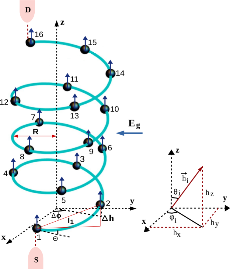
Figure 1: (Color online). Left panel: schematic diagram of a right-handed helical geometry, coupled to source and drain electrodes, having radius $R$, stacking distance $\Delta h$, twisting angle $\Delta\phi$, helix angle $\Theta$ and nearest-neighbor distance $l_{1}$. Each site $i$ of the system contains a finite magnetic moment which is responsible for spin dependent scattering through the interaction of the injected electron spin with the net spin $\langle\vec{S}_{i}\rangle$ located at $i$th site. We define this scattering parameter as $\vec{h}_{i}$. An external electric field $E_{g}$ is applied to the system, along the perpendicular direction of the helix axis, by placing it within suitable gate electrodes. Right panel: general arrangement of $\vec{h}_{i}$ associated with the net spin at $i$th site, where $\theta_{i}$ and $\varphi_{i}$ are the polar and azimuthal angles, respectively.

If $\langle\vec{S}_{i}\rangle$ be the net spin at the magnetic site $i$, then we can define the spin-dependent scattering parameter at $i$th site as $\vec{h}_{i}=J\langle\vec{S}_{i}\rangle$ spsp . The orientation of $\vec{h}_{i}$, associated with the orientation of $\langle\vec{S}_{i}\rangle$ is described by the polar angle $\theta_{i}$ and azimuthal angle $\varphi_{i}$ (right panel), as used in conventional spherical polar co-ordinate system. These magnetic sites are responsible for spin dependent scattering. The parameters $\Delta h$ and $\Delta\phi$, describing the stacking distance and twisting angle respectively, play important roles to characterize whether the long-range or short-range hopping is important, and at the same time determines the structure of the magnetic helix. When $\Delta h$ is too small i.e., the atoms are closely spaced, electrons can hop to different sites of the geometry yielding a long-range hopping (LRH) helix, while for the other situation when $\Delta h$ is reasonably large the system maps to the short-range hopping (SRH) helix. As already stated, depending on $\Delta h$ and $\Delta\phi$, the hopping of electrons as well as the helical structure get modified which can be more clearly understood from our forthcoming analysis. We will examine the effects of all these factors on spin selective transmission in detail for the comprehensive analysis.

In order to describe the Hamiltonian of the magnetic helix sandwiched between S and D (left panel of Fig. 1), a tight-binding (TB) framework is given. In presence of magnetic interaction mh1 ; mh2 ; mh3 ; mh4 , the TB Hamiltonian of a right-handed magnetic helix having $N$ sites reads as,

$$H_{\mbox{\tiny mh}} = \sum_{i}\mbox{\boldmath{$c$}}_{i}^{\dagger}\left(\mbox{\boldmath{$\epsilon$}}_{i}-\mbox{\boldmath{$h$}}_{i}.\mbox{\boldmath{$\sigma$}}\right)\mbox{\boldmath{$c$}}_{i}$$ (1)

$$+ \sum_{i=1}^{N-1}\sum_{j=1}^{N-i}\left(\mbox{\boldmath{$c$}}_{i}^{\dagger}\mbox{\boldmath{$t$}}_{j}\mbox{\boldmath{$c$}}_{i+j}+\mbox{\boldmath{$c$}}_{i+j}^{\dagger}\mbox{\boldmath{$t$}}_{j}^{\dagger}\mbox{\boldmath{$c$}}_{i}\right)$$

where, $\mbox{\boldmath{$c$}}_{i}=\begin{pmatrix}c_{i\uparrow}\\ c_{i\downarrow}\end{pmatrix}$, $\mbox{\boldmath{$c$}}_{i}^{\dagger}=\begin{pmatrix}c_{i\uparrow}^{\dagger}&c_{i\downarrow}^{\dagger}\end{pmatrix}$, $\mbox{\boldmath{$\epsilon$}}_{i}=\begin{pmatrix}\epsilon_{i}&0\\ 0&\epsilon_{i}\end{pmatrix}$, $\mbox{\boldmath{$t$}}_{j}=\begin{pmatrix}t_{j}&0\\ 0&t_{j}\end{pmatrix}$, and $\mbox{\boldmath{$h$}}_{i}.\mbox{\boldmath{$\sigma$}}=h_{i}\begin{pmatrix}\cos\theta_{i}&\sin\theta_{i}e^{-k\varphi_{i}}\\ \sin\theta_{i}e^{k\varphi_{i}}&-\cos\theta_{i}\end{pmatrix}$. The term ($\mbox{\boldmath{$\epsilon$}}_{i}-\mbox{\boldmath{$h$}}_{i}.\boldsymbol{\sigma}$) represents the effective site energy matrix, where $\epsilon_{i}$ is the on-site energy in absence of any magnetic interaction, and $\mbox{\boldmath{$h$}}_{i}.\mbox{\boldmath{$\sigma$}}$ is the spin dependent scattering factor which appears due to the presence of magnetic moments at each lattice sites of the geometry. $\mbox{\boldmath{$\sigma$}}=(\sigma_{x},\sigma_{y},\sigma_{z})$ is the Pauli spin vector with the component $\sigma_{z}$ in diagonal representation. $c_{i\sigma}^{\dagger}$ and $c_{i\sigma}$ are the usual fermionic creation and annihilation operators, respectively, at $i$th site of spin $\sigma$ ($\uparrow,\downarrow$). The meanings of $\theta_{i}$ and $\varphi_{i}$ are already described above, and here $k$ corresponds to $\sqrt{-1}$. The parameter $t_{j}$ is associated with the electron hopping between the sites $i$ and ($i+j$), and it is expressed as qfs3 $t_{j}=t_{1}e^{-(l_{j}-l_{1})/l_{c}}$, where $t_{1}$ gives the nearest-neighbor hopping (NNH) integral, $l_{1}$ represents the nearest-neighbor distance (see Fig. 1), and $l_{c}$ denotes the decay constant. The distance $l_{j}$ between the sites $i$ and ($i+j$) is written in terms of the radius $R$, twisting angle $\Delta\phi$, and stacking distance $\Delta h$ as qfs3 $l_{j}=\sqrt{[2R\sin(j\Delta\phi/2)]^{2}+(j\Delta h)^{2}}$.

Now, in presence of an external electric field $E_{g}$, perpendicular to the helix axis, the site energy of the helical geometry gets modified efl and it becomes

$$\epsilon_{i}=\epsilon_{i}^{0}+eV_{g}\cos\left(i\Delta\phi-\beta\right)$$ (2)

where $\epsilon_{i}^{0}$ is the site energy in absence of $E_{g}$, and $V_{g}$ is the gate voltage which is related to $E_{g}$ as $2V_{g}=2E_{g}R$ ($R$ being the radius, see Fig. 1). The phase factor $\beta$ is associated with the electric field direction. It measures the angle between the incident electric field and the positive $X$ axis. This phase can be changed quite easily either by rotating the helical geometry or by changing the positions of the gate electrodes (for schematic illustration of this kind of electric field, see Ref. efl ).

This is all about the TB Hamiltonian of the magnetic helix. Now we describe the TB Hamiltonians of the other parts of the junction i.e., the contact electrodes S and D and their coupling with the MH. The electrodes are assumed to be perfect, reflection-less, non-magnetic and semi-infinite. Considering the site energy and NNH integrals (long-range hopping is not considered in the electrodes) as $\epsilon_{0}$ and $t_{0}$, respectively, we can express the TB Hamiltonians as

$$H_{\mbox{\tiny S}}=\sum_{m<1}\mbox{\boldmath{$a$}}_{m}^{\dagger}\mbox{\boldmath{$\epsilon$}}_{0}\mbox{\boldmath{$a$}}_{m}+\sum_{m<1}(\mbox{\boldmath{$a$}}_{m}^{\dagger}\mbox{\boldmath{$t$}}_{0}\mbox{\boldmath{$a$}}_{m-1}+h.c.)$$ (3)

and

$$H_{\mbox{\tiny D}}=\sum_{m>N}\mbox{\boldmath{$b$}}_{m}^{\dagger}\mbox{\boldmath{$\epsilon$}}_{0}\mbox{\boldmath{$b$}}_{m}+\sum_{m>N}(\mbox{\boldmath{$b$}}_{m}^{\dagger}\mbox{\boldmath{$t$}}_{0}\mbox{\boldmath{$b$}}_{m+1}+h.c.)$$ (4)

where $\mbox{\boldmath{$\epsilon$}}_{0}$ and $\mbox{\boldmath{$t$}}_{0}$ are the ($2\times 2$) diagonal matrices, and the forms of $\mbox{\boldmath{$a$}}_{m}$ and $\mbox{\boldmath{$b$}}_{m}$ are similar to what is described above for $\mbox{\boldmath{$c$}}_{i}$. The operators ($a_{m\sigma}^{\dagger}$, $a_{m\sigma}$) and ($b_{m\sigma}^{\dagger}$, $b_{m\sigma}$) are the usual fermionic operators used for source and drain electrodes.

These electrodes are directly coupled at the two extreme points of the helical geometry as shown in Fig. 1. In terms of the coupling strengths $t_{S}$ and $t_{D}$ due to source and drain, respectively, the TB coupling Hamiltonian looks like

$$H_{\mbox{\tiny cpl}}=\mbox{\boldmath{$a$}}_{0}^{\dagger}\mbox{\boldmath{$t$}}_{S}\mbox{\boldmath{$c$}}_{1}+\mbox{\boldmath{$c$}}_{N}^{\dagger}\mbox{\boldmath{$t$}}_{D}\mbox{\boldmath{$b$}}_{N+1}+h.c.$$ (5)

where $\mbox{\boldmath{$t$}}_{S}$ and $\mbox{\boldmath{$t$}}_{D}$ are the ($2\times 2$) diagonal matrices.

II.2 Theoretical prescription

To compute spin dependent transport quantities we use Green’s function formalism, a standard and suitable technique for such calculations gf1 . The fundamental quantity that is first required to determine is the two-terminal transmission function. In terms of coupling matrices $\mbox{\boldmath{$\Gamma$}}_{S}^{\sigma}$ and $\mbox{\boldmath{$\Gamma$}}_{D}^{\sigma^{\prime}}$, the transmission function becomes gf1 ; gf2 ; gf3

$$T_{\sigma\sigma^{\prime}}=\mbox{Tr}\left[\mbox{\boldmath{$\Gamma$}}_{S}^{\sigma}\mbox{\boldmath{$G$}}^{r}\mbox{\boldmath{$\Gamma$}}_{D}^{\sigma^{\prime}}\mbox{\boldmath{$G$}}^{a}\right]$$ (6)

where $\mbox{\boldmath{$\Gamma$}}_{S(D)}^{\sigma(\sigma^{\prime})}=-2\mbox{Im}\left[\mbox{\boldmath{$\Sigma$}}_{S(D)}^{\sigma(\sigma^{\prime})}\right]$. $\mbox{\boldmath{$\Sigma$}}_{S(D)}^{\sigma}$ is the contact self-energy due to source (drain) electrode, which incorporates the effect of contact electrode. The factors $\mbox{\boldmath{$G$}}^{r}$ and $\mbox{\boldmath{$G$}}^{a}$ are the retarded and advanced Green’s functions, respectively, and they are determined via the relations gf1 $\mbox{\boldmath{$G$}}^{r}=(\mbox{\boldmath{$G$}}^{a})^{\dagger}=\left[E\mbox{\boldmath{$I$}}-H_{\mbox{\tiny mh}}-\boldsymbol{\Sigma}_{S}^{\sigma}-\boldsymbol{\Sigma}_{D}^{\sigma}\right]^{-1}$, where $I$ is the identity matrix having dimension ($2N\times 2N$). $T_{\sigma\sigma^{\prime}}$ describes the probability of a transmitted electron with spin $\sigma^{\prime}$ that is injected with spin $\sigma$. Thus, for $\sigma=\sigma^{\prime}$, we get pure spin transmission, while for the other case ($\sigma\neq\sigma^{\prime}$) spin-flip transmission is obtained. We define the net up and down spin transmission probabilities as: $T_{\uparrow}=T_{\uparrow\uparrow}+T_{\downarrow\uparrow}$ and $T_{\downarrow}=T_{\downarrow\downarrow}+T_{\uparrow\downarrow}$.

Determining spin dependent transmission probabilities, we can easily calculate different spin dependent currents by integration procedure of the transmission function over a suitable energy window associated with bias voltage $V$. At zero temperature, the current expression becomes gf1

$$I_{\sigma\sigma^{\prime}}=\displaystyle\frac{e}{h}\int\limits_{E_{F}-\frac{eV}{2}}^{E_{F}+\frac{eV}{2}}T_{\sigma\sigma^{\prime}}(E)\,dE$$ (7)

where $e$ and $h$ are the fundamental constants, and $E_{F}$ is the equilibrium Fermi energy. Since the broadening of energy levels due to the coupling of the MH with the contact electrodes is too large compared to the thermal broadening gf1 , we can safely ignore the effect of temperature in our present analysis.

Using spin dependent currents, we eventually compute spin polarization coefficient from the relation mh4 ; pola1

$$P=\frac{I_{\uparrow}-I_{\downarrow}}{I_{\uparrow}+I_{\downarrow}}$$ (8)

where $I_{\uparrow}=I_{\uparrow\uparrow}+I_{\downarrow\uparrow}$ and $I_{\downarrow}=I_{\downarrow\downarrow}+I_{\uparrow\downarrow}$. $P=0$ means no polarization, whereas $P=\pm 1$ corresponds to $100\%$ spin polarization.

Finally, to include the effect of helical dynamics within the framework of TB approximation, we follow the prescription as originally put forward by Ratner and co-workers hd2 , an elegant and simple idea to incorporate the dynamics of a system. The site energy of a particular site of the magnetic helix, where the drain electrode is coupled, gets modified by adding an imaginary part $-k\hbar/\tau$ (i.e., $\epsilon_{i}\rightarrow\epsilon_{i}-k\hbar/\tau$, $k=\sqrt{-1}$). The parameter $\tau$ represents the decay time, and its value should be chosen in such a way that the electron vanishes immediately when it will reach to the drain end, and at the same time emphasis should be given that it cannot be so small that wave function gets reflected from the end site hd2 .

III Numerical Results and discussion

In what follows we present our essential results of spin dependent transport. The key aspects that we want to explore are: (i) the interplay between SRH and LRH interactions on transport phenomena, (ii) the CISS effect and (iii) the helical dynamics on spin selective transmission. Unless stated, we select the physical parameters in such a way that we can have two different magnetic helix systems: one associated with the long-range hopping and the other associated with the short-range one. If not specified, we choose the parameters for the right-handed LRH MH as $R=2.5\,$Å, $\Delta h=1.5$Å and $\Delta\phi=5\pi/9$, while these parameters for the right-handed SRH MH are: $R=7$Å, $\Delta h=3.4$Å and $\Delta\phi=\pi/5$. The decay exponent is fixed as $l_{c}=0.9$Å. These parameters are equivalent to the DNA and $\alpha$-helical protein molecules, the suitable examples of SRH and LRH models as already established in literature rps . Along with the interplay between two kinds of hopping of electrons, in the present work we also consider both the right- and left-handed magnetic helices to explore the strong CISS effect. As it is already stated earlier that depending on $\Delta h$ and $\Delta\phi$, the structure of the MH also gets changed together with the hopping. To reveal this fact look into the spectra given in Fig. 2.

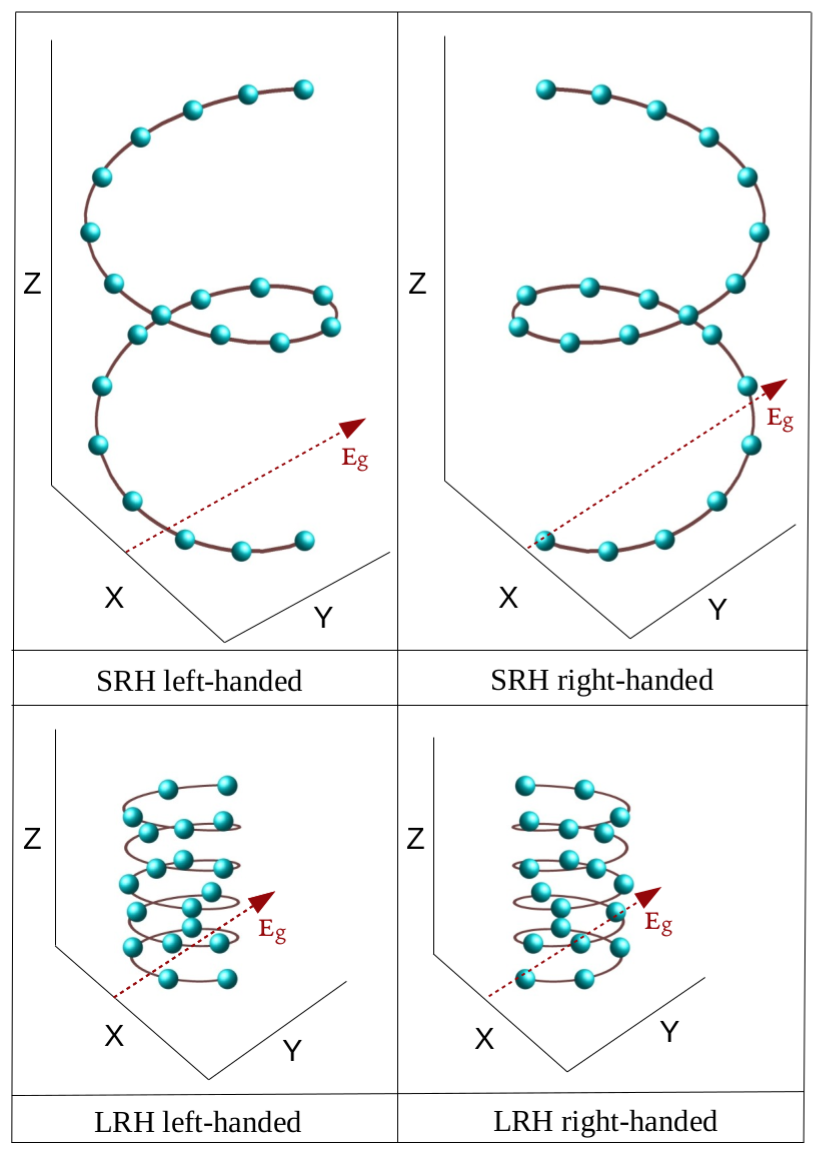
Figure 2: (Color online). Both right-handed and left-handed magnetic helices under two different hopping conditions.

What we see is that, for the chosen set of parameter values, the short-range hopping takes place along the MH with about two turn when $N=21$, while about five turns occurs in the case of long-range hopping if we set $N=19$. It clearly demonstrates the structural change of the helical geometry, and we explore these issues in spin selective electron transmission.

The other common parameters that we use throughout the analysis are as follows. The on-site energy and NNH integrals, $\epsilon_{0}$ and $t_{0}$, in the contact electrodes are fixed at zero and $4$ respectively, and these electrodes are connected to the MH with the strength $t_{S}=t_{D}=0.8$. The field-independent site energy $\epsilon_{i}^{0}$ in the MH is set at zero, without loss of any generality, and we fix $t_{1}=1$. Unless specified, we fix the system size $N=20$. For the sake of simplification, we set the polar and azimuthal angles to zero, and under this condition no spin-flip transmission is available. In our numerical calculations, the left-handed helix is obtained by changing $\Delta\phi$ to $-\Delta\phi$ gc5 , and if not mentioned we present the results of right-handed magnetic helices. Finally, we consider the magnitude of spin-dependent interaction parameter $h_{i}=1\,$eV $\forall\,i$. All the other energies are also measured in unit of electron volt (eV). Here it is important to note that the magnitude of $\vec{h}_{i}$ ($=J\langle\vec{S}_{i}\rangle$) cab be even much higher than $1\,$eV due to the strong coupling spsp (defined by the strength $J$) between the spin of an incoming electron with the net spin $\langle\vec{S}_{i}\rangle$ of the local magnetic sites in the magnetic helix. This is one of the key advantage of getting strong spin-dependent scattering in a magnetic material compared to the spin-orbit coupled systems spsp .

III.1 Interplay between SRH and LRH interactions on transport phenomena

To unravel the basic mechanism of electron transport through any conducting junction, it is always helpful to start with analyzing the nature of transmission function for the junction setup. The results shown in Fig. 3 describe the spin dependent transmission probabilities for the LRH and SRH magnetic helices. For the time being we fix the external electric field to zero, and its effect will be considered in the subsequent sections. Several notable features are observed from Fig. 3 which we describe one by one as follows. A distinct feature in the arrangements of resonant transmission peaks, associated with the energy eigenvalues of the MH, can be observed in the short-range and long-range hopping helical geometries. For the SRH MH, the resonant peaks are almost uniformly arranged and their widths are nearly identical. This behavior is quite analogous to the conventional NNH model. On the other hand, for the other MH with LRH integrals, the resonant peaks are densely packed in one side (left one), whereas they are widely separated in the other side of the $T_{\sigma}$-$E$ spectrum (upper row of Fig. 3). This is

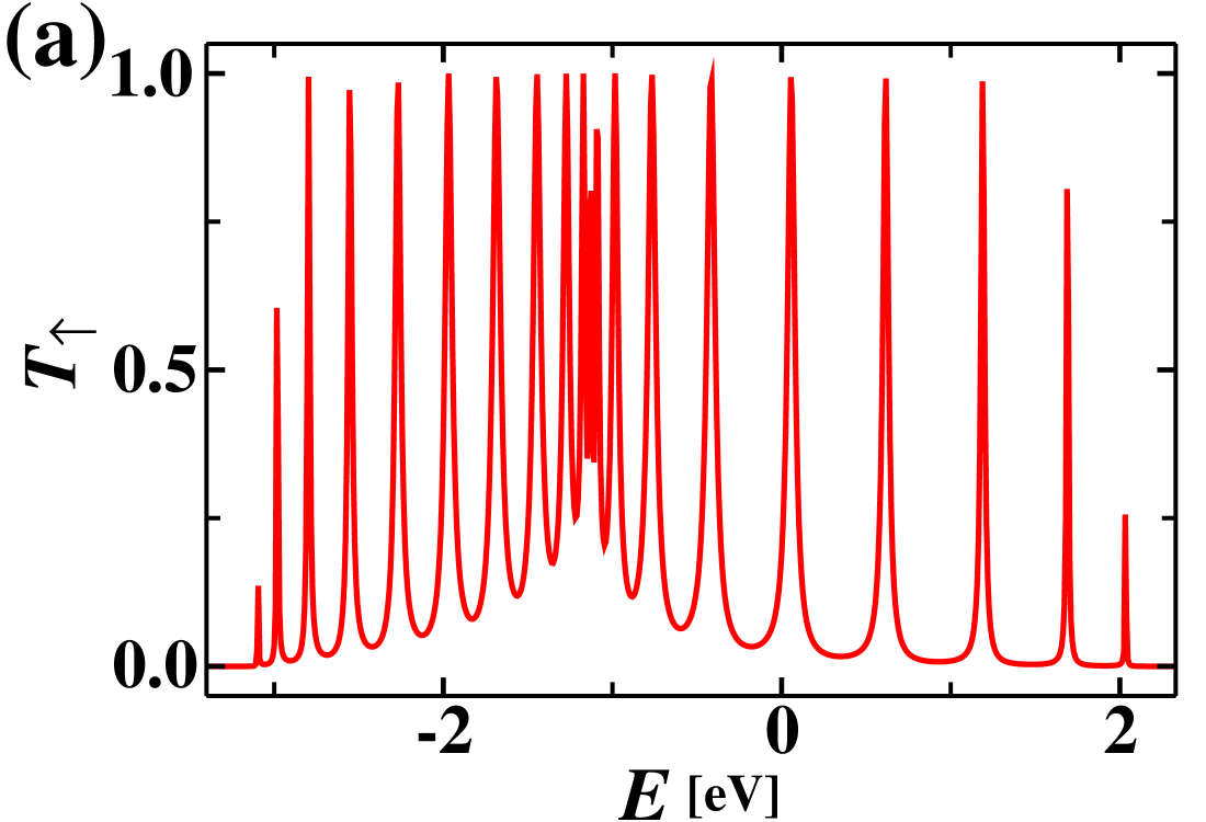
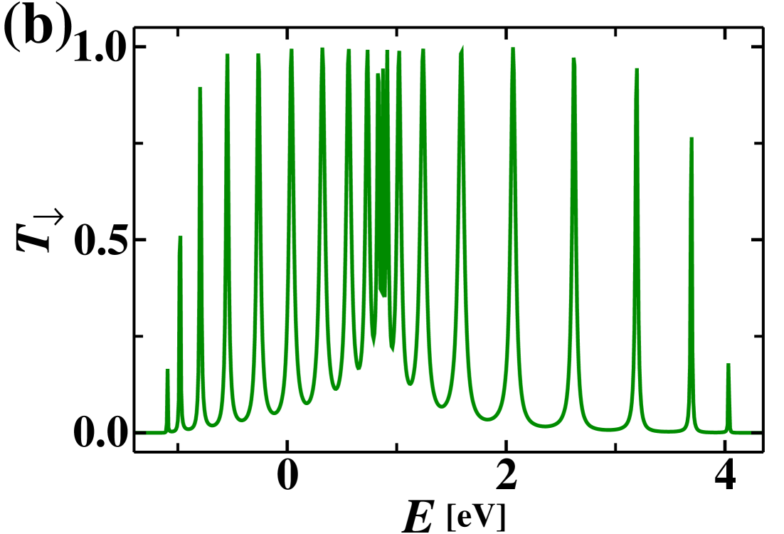
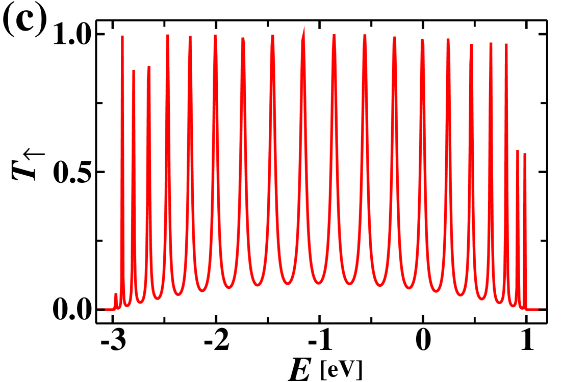
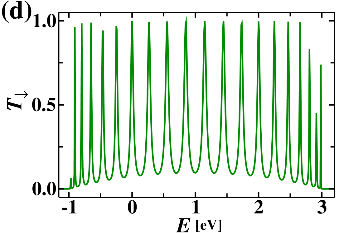
Figure 3: (Color online). Up and down spin transmission probabilities as a function of injecting electron energy $E$ for a MH in absence of any electric field where the top and bottom rows correspond to the LRH and SRH magnetic helices, respectively.

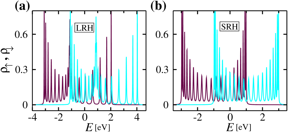
Figure 4: (Color online). Density of states of up (maroon color) and down (cyan color) spin electrons for the identical magnetic helix systems as taken in Fig. 3.

the generic feature of LRH model emphasizing the breaking of particle-hole symmetry, unlike the NNH case where such symmetry is no longer violated. The nature of short or long-range hopping of electrons can be visualized by noting the distances between different neighbor sites. For the chosen set of parameter values if we calculate the distances between first few neighbors then they will look like (in unit of $\AA$) for the LRH MH as: $l_{1}=4.113$, $l_{2}=5.766$, $l_{3}=5.148$, $l_{4}=6.239$, $l_{5}=8.850$, $\dots$, while for the SRH one they are: $l_{1}=5.502$, $l_{2}=10.675$, $l_{3}=15.242$, $l_{4}=19.033$, $l_{5}=22.023$, $\dots$, etc. As the neighboring distances increase so rapidly for the SRH helix, electrons are no longer able to hop into far away sites, and the contributions essentially restricted within the too few neighboring sites.

Now, due to the existence of spin dependent scattering term in the MH, as prescribed in Eq. 1, a finite shift in energy scale between the up and down spin transmission spectra takes place, associated with the two spin channels. Thus, naturally when the Fermi energy is fixed anywhere within the region where only up or down spin transmission probability is finite, we can get pure up or down spin propagation through the junction yielding $100\%$ polarized spin current. This fact is quite well-known in literature in the context of spin polarization considering a magnetic material. But, the interesting thing is that due to non-uniform distribution of $T_{\sigma}$-$E$ spectrum across its center for the case of LRH MH (upper row of Fig. 3), a significantly large spin polarization will be achieved even when the Fermi energy is placed within the overlap region between the two spin channels. This phenomenon, viz high degree of polarization, cannot be observed for the case of SRH helix, due to regular distribution of transmission functions where both up and down spin electrons contribute almost in equal amounts. The other key advantage of getting large spin polarization towards the band center is that experimentally it will be quite

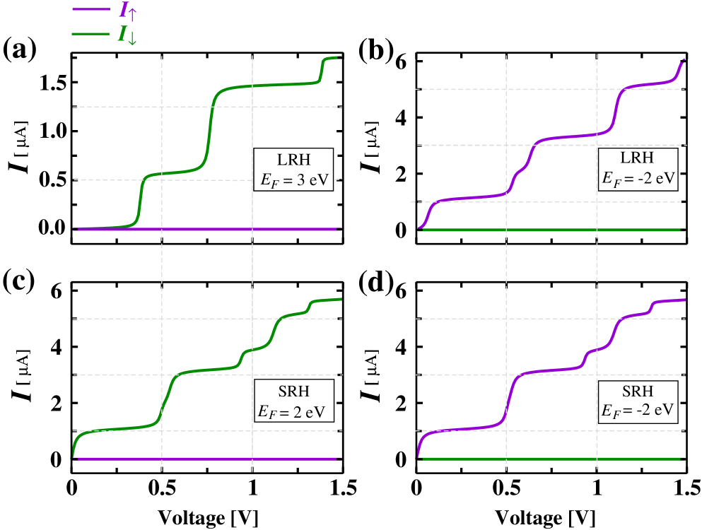
Figure 5: (Color online). Current-voltage characteristics for the LRH and SRH magnetic helix structures at some typical values of $E_{F}$, in the absence of external electric field.

easier to place the Fermi energy and it can be tuned as well in these energy regions, rather than the placing of $E_{F}$ near the band edge. Thus, the LRH MH is relatively superior than the SRH one, and more favorable justification for this statement can be found from our forthcoming analysis.

The origin of the finite shift of up and down spin transmission spectra along with the overlap of these two spin bands, and the position of different transmission peaks in the LRH and SRH magnetic helices can be understood in a more transparent way by noting the density of states (DOS) spectra of different spin electrons for these magnetic helix structures. This is due to the fact that the transmission function is directly related to the energy spectrum and thus DOS. We compute DOS following the well-known relation $\rho_{\sigma}(E)=-(1/N\pi)\mbox{Im}[\mbox{Tr}(\mbox{\boldmath{$G$}}_{\sigma}^{r})]$. Figure 4 shows the DOS profiles for the up and down spin electrons for the identical magnetic helix structures as considered in Fig. 3. From the spectra it is noticed that a finite shift in energy scale takes place between the two spin bands with a suitable overlap among them. At the same time the alignments of different peaks along with their separations for the two different hopping cases are also nicely emerged. These features are exactly evolved in the transmission spectra (Fig. 3).

The above nature of transmission function is directly reflected in current-voltage characteristics. As illustrative examples, in Fig. 5 we show the variation of spin dependent currents as a function of bias voltage $V$ at some typical Fermi energies. Here we also consider the zero-field case

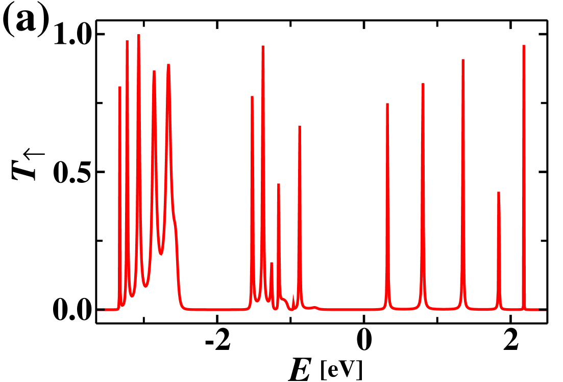
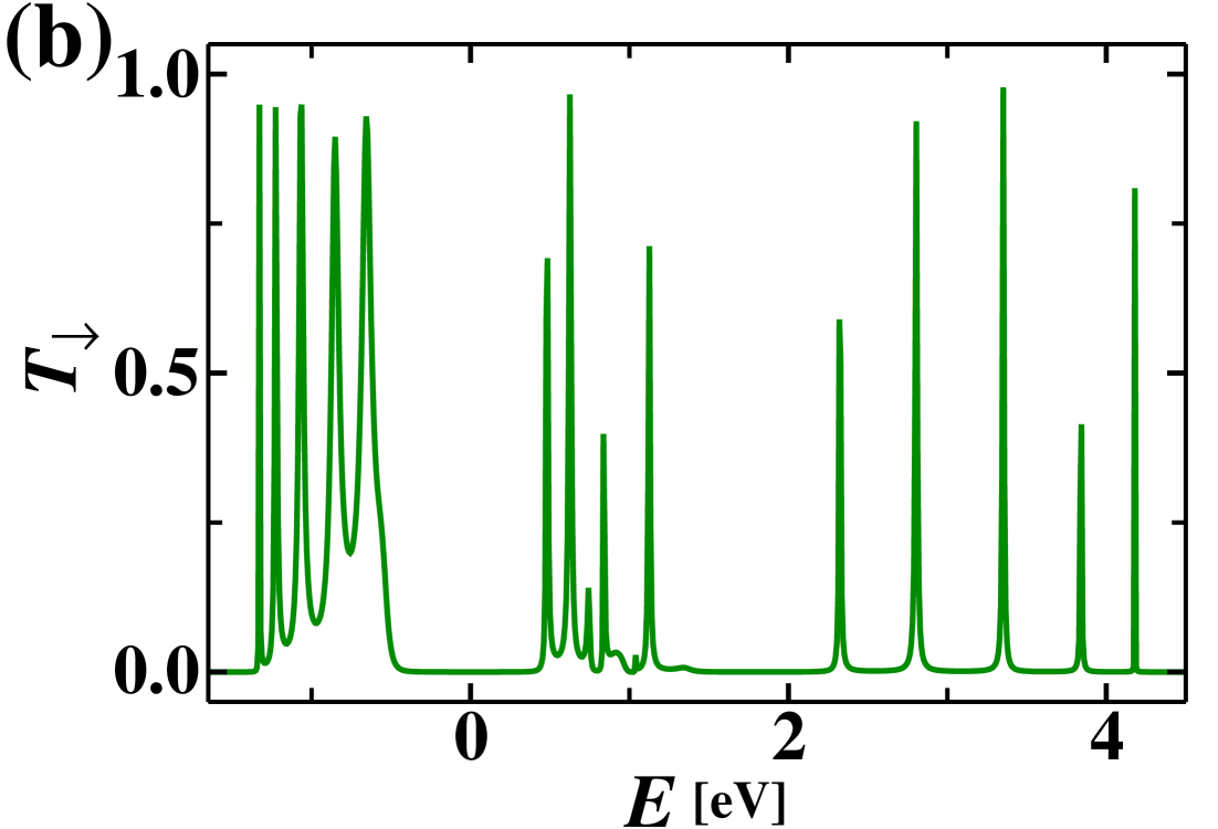
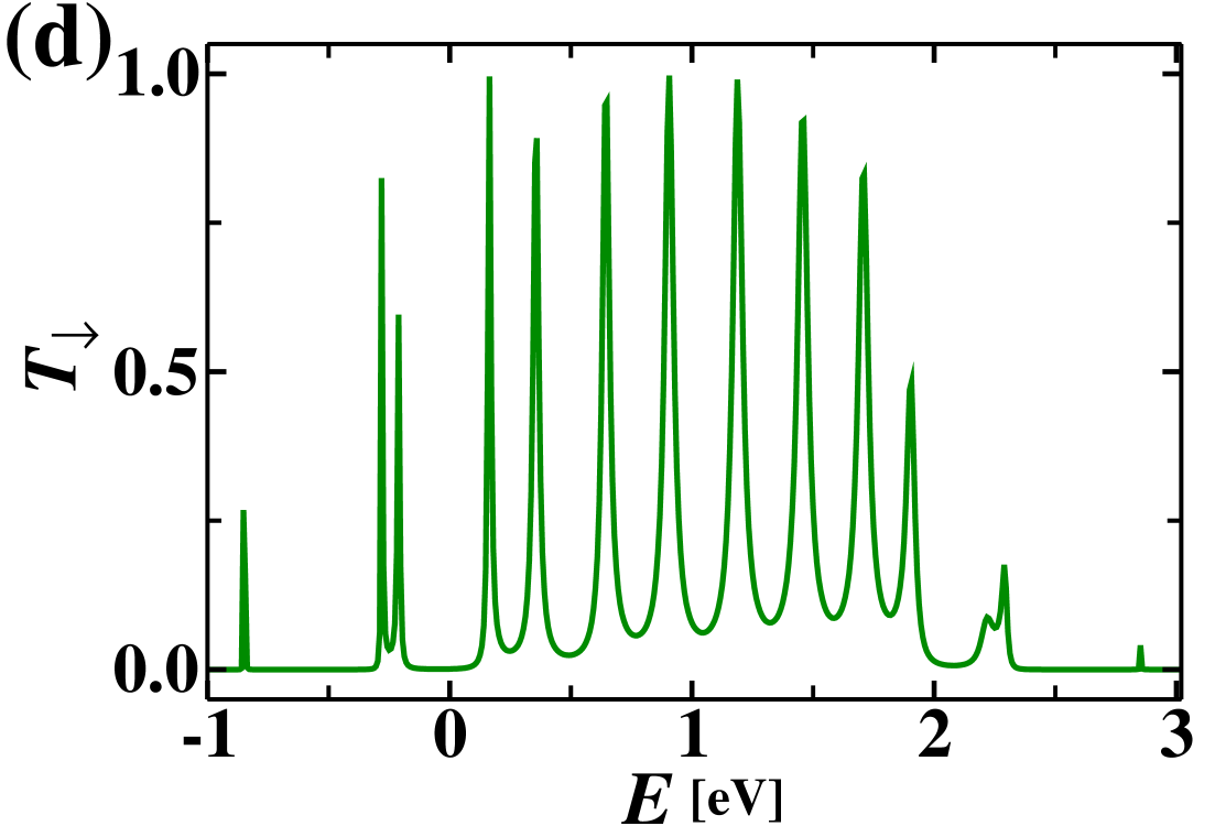
Figure 6: (Color online). Up and down spin transmission probabilities in presence of external gate voltage $V_{g}$ that produces the electric field $E_{g}$ where the top and bottom rows correspond to the LRH and SRH helices, respectively. Here we set $V_{g}=1\,$V.

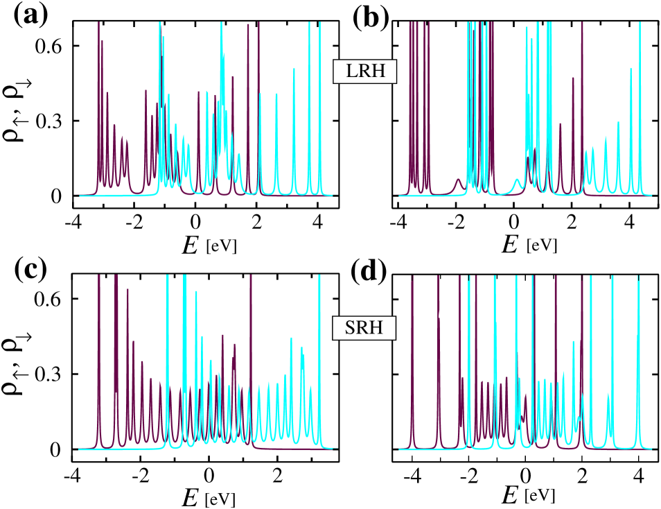
Figure 7: (Color online). Density of states for up (maroon color) and down (cyan color) spin electrons in presence of external gate voltage where the first column corresponds to $V_{g}=0.5\,$V and $\beta=0$, and the second column represents $V_{g}=1.5\,$V and $\beta=\pi/2$.

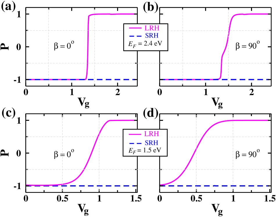
Figure 8: (Color online). Spin polarization $P$ as a function of gate voltage $V_{g}$ at some typical values of $\beta$ for two different Fermi energies considering the bias voltage $V=0.2\,$V.

like Fig. 3, to visualize the reflectance of $T_{\sigma}$-$E$ spectra on $I_{\sigma}$-$V$ characteristics. The voltage window and the Fermi energies are chosen selectively so that only one spin electrons can propagate through the junction. Thus, for this entire bias window ($0<V<1.5\,$V), which is reasonably large, only up or down spin electrons propagates yielding a $\pm 100\%$ spin polarized current. For the LRH MH, a distinct feature in current steps is observed for the two different choices of Fermi energies, $E_{F}=-2\,$eV and $E_{F}=3\,$eV. And the other notable thing is that the magnitudes of the currents are largely different, that can be visualized by comparing the results shown by the green line in Fig. 5(a) and magenta line in Fig. 5(b). These features are solely associated with the transmission spectra (see the upper row of Fig. 3), as the current is evaluated by the integration procedure of the transmission function. On the other hand, for the SRH MH, the currents are almost comparable to each other (green curve in Fig. 5(c) and magenta curve in Fig. 5(d)), following the uniform distribution of transmission peaks.

From the zero-field spin dependent transmission probabilities (Fig. 3) and currents (Fig. 5) we already get some suitable hints about the interplay between the two kinds of hopping integrals on spin selective transmission. Now, in the remaining parts we include the effects of external electric field to explore several more interesting features in the magnetic helix geometry. Like above, here also we start with the variation of transmission function with energy $E$. The results are shown in Fig. 6. In the presence of electric field, the system behaves like a correlated disordered one cor1 ; cor2 and therefore the transmission spectrum is no longer symmetric even for the short-range hopping magnetic helix. The key feature is that, the transmission spectrum is gapped cor1 ; cor2 ; fra1 ; fra2 associated with the energy spectrum of the MH, and it is more prominent when we consider longer-range hopping of electrons. Due to this gapped spectrum, there is a finite probability to have non-zero transmission of one spin electrons at multiple energy zones, even not far away from the band center, while completely vanishing transmission for the other spin electrons. Under this situation we can get $100\%$ polarized spin current. The width of these gaps and at the same time swapping of contributing channel can also be tuned with the help of $V_{g}$ as well as phase factor $\beta$ that we confirm through our exhaustive calculations.

The gapped nature of the transmission functions and their possible tuning by means of $V_{g}$ and $\beta$ can be understood easily by noting the density of states (DOS) profiles under different input conditions of these

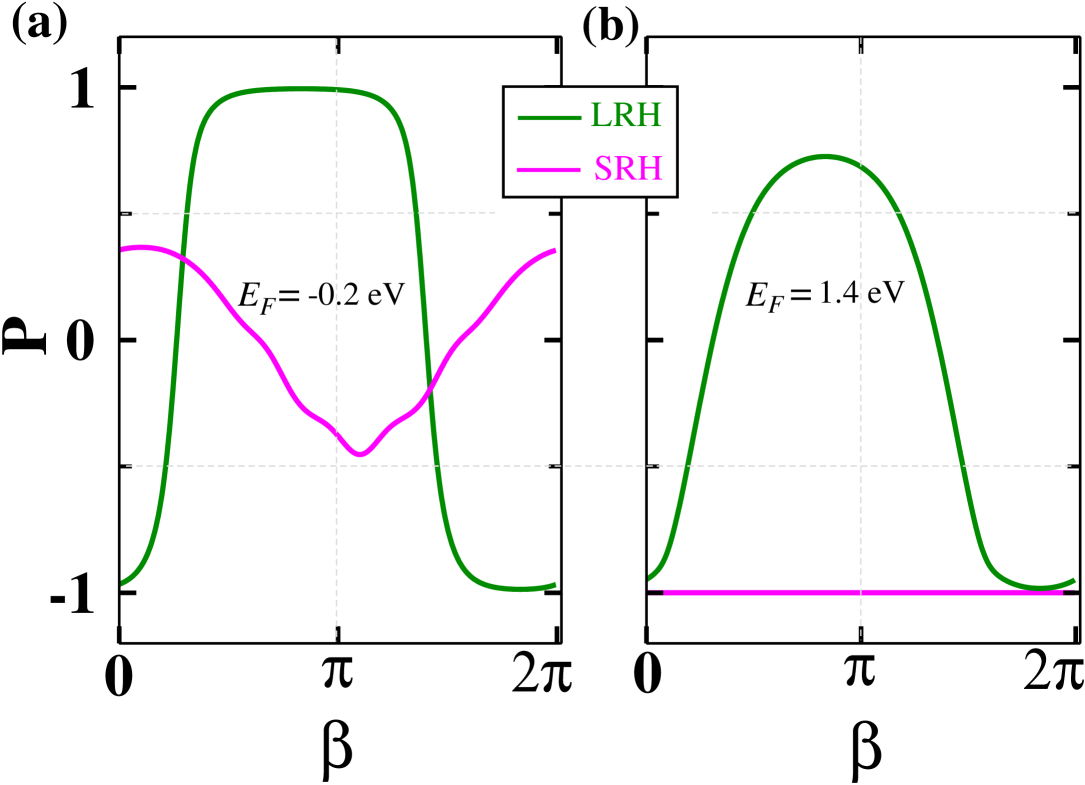
Figure 9: (Color online). Dependence of spin polarization $P$ with phase factor $\beta$ at two different Fermi energies. Here we fix $V_{g}=0.5\,$V and $V=0.2\,$V.

physical parameters, as the transmission spectrum is directly related to the energy spectrum and thus the DOS. Figure 7 displays the DOS spectra for up and down spin electrons at some typical values of $V_{g}$ and $\beta$. Prominent bands, separated by sharp gaps, are obtained for the LRH MH, whereas the effects are

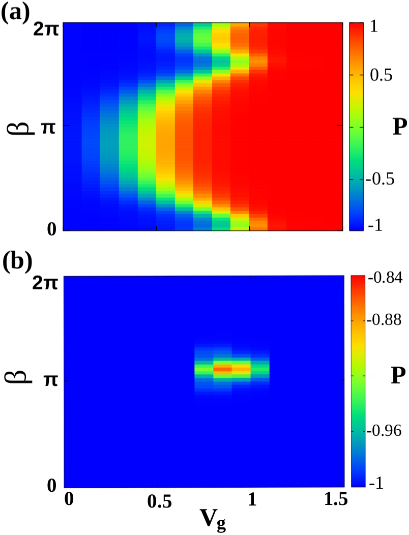
Figure 10: (Color online). Simultaneous variation of $P$ with $V_{g}$ and $\beta$ for the (a) LRH and (b) SRH helices, considering $V=0.2\,$V and $E_{F}=1.5\,$eV.

comparatively less for the SRH helix. The shifting of different peaks with the inclusion of $\beta$ is clearly visible. The transmission functions corroborate these behaviors what are shown in Fig. 6.

These facts can be validated further from the results presented in Fig. 8, where the dependence of spin polarization $P$ is shown as a function of gate voltage for some typical values of phase factor $\beta$ at two Fermi energies. The bias voltage $V$ is fixed at $0.2\,$V. From all the spectra it is clearly seen that much higher spin polarization can be obtained, and in some cases it reaches to $100\%$, by varying $V_{g}$. The notable feature is that a perfect phase reversal of spin polarization i.e., $-100\%$ to $+100\%$ can be done by regulating the gate voltage. This is a clear signature of externally tuning selective spin transmission using a magnetic helix structure.

The above discussion raises an obvious question that as the change of site energy, due to the variation of $V_{g}$, leads to a significant change in

Figure 11: (Color online). Effect of system size $N$ on spin polarization $P$. Here we choose $V=0.2\,$V.

transmission spectra, and thus, spin polarization, can we also expect any non-trivial signature of selective spin transmission by tuning the phase factor $\beta$ for a constant $V_{g}$, as it is directly involved in site energy (see Eq. 2). To explore it, let us focus on the spectra given in Fig. 9, where the variation of $P$ as a function of $\beta$ is shown for two typical Fermi energies. The results are computed setting $V_{g}=0.5\,$V and $V=0.2\,$V. For the SRH MH a minor variation of $P$ is noticed with $\beta$, whereas a significantly large change in $P$ is possible for the LRH MH, which again proves the superiority of LRH MH compared to the other one. The underlying mechanism is same as noted earlier that the contributing spin channels are modified with the modulation of site energy. Thus, for a fixed gate voltage, selective spin polarization can be achieved simply by changing the orientation of incident electric field. This is a more suitable way of tuning spin transport compared to the other proposals where usually magnetic field plays this role.

To test the sensitivity of $P$ on both the gate voltage and phase factor, in Fig. 10 we plot the simultaneous variation of $P$ with $V_{g}$ and $\beta$, considering $V=0.2\,$V and $E_{F}=1.5\,$eV. A drastic change is clearly visible between the LRH and SRH helices. The spin polarization $P$ is almost insensitive for a wide range of both $V_{g}$ and $\beta$ in the case of SRH MH, where it varies very close to $-1$. On the other hand, for the other situation, a complete phase reversal of $P$ is possible, and each of these two phases ($P=+1$ or $P=-1$) persists over a wide range of parameter values, which thus gives us a confidence to examine the results in laboratory.

In this context it is also relevant to examine the role of system size $N$. The results are presented in Fig. 11 for two specific values of $V_{g}$ setting the voltage bias at $0.2\,$V. In the case of long-range hopping magnetic helix, large oscillation is observed for smaller $N$, and it is gradually dying out with $N$. While, a finite oscillation with almost constant amplitude is exhibited for the case of short-range hopping helix. The strong modulation of spin polarization with helix size $N$ appears due to the quantum interference of electronic waves, and this effect is again directly related to the incomplete helix nature with the change of $N$.

III.2 CISS effect

It is well known that a simple ferromagnetic material exhibits spin filtration effect. This is quite trivial and extensively studied in

Figure 12: (Color online). Spin polarization coefficient $P$ as function of gate voltage $V_{g}$ for the left- and right-handed helical geometries. We set $N=19$ and $21$, respectively, for the LRH and SRH magnetic helices, to have the full turns. The other physical parameters are: bias voltage $V=0.2\,$V and the phase factor $\beta=\pi/2$.

literature. But, the magnetic helix geometry which we consider here in our work is completely a new configuration, as it exhibits strong CISS effect, analogous to what was discussed by some pioneering groups in their works ghl ; ciss1 ; ciss2 ; ciss3 ; ciss4 ; ciss5 . To the best of our knowledge, no one has explored the CISS effect in any MH geometry so far.

To reveal the helicity effect on spin polarization, let us look into the spectra given in Fig. 12 where we show the variation of $P$ on gate voltage $V_{g}$, for the left-handed (LH) and right-handed (RH) helical geometries. The results are computed for exactly two opposite helcities, keeping all the other parameters unchanged, where (a) and (b) correspond to the LRH and SRH helices, respectively. To get the magnetic helix with full number of turns (which is extremely important to examine the CISS effect and compare the results between two different handed helical geometries), here we take $N=19$ for the long-range hopping MH, while it ($N$) becomes $21$ for the short-range MH. The spin polarization changes drastically with the handedness, as clearly seen by comparing the two colored curves. It becomes more prominent for the SRH model compared to the LRH one. Almost a complete phase reversal of $P$ takes place upon the alteration of the helical sense. The nature of polarization with the change of handedness is solely associated with the contributing up and down spin channels within the selected energy window around $E_{F}$, associated with the bias voltage. For the short-range helix, almost perfect swapping takes place between the up and down spin transmission probabilities upon the inversion of handedness, which results nearly full inversion of spin polarization. On the other hand, for the long-range hopping helix, the transmission probabilities are largely asymmetric and perfect swapping is no longer possible, and thus, we do not get the complete phase reversal of $P$ for the opposite handed helix geometry, like what we see in the case of short-range helix system.

Keeping the handedness (right- or left-handed) of the MH fixed, we can

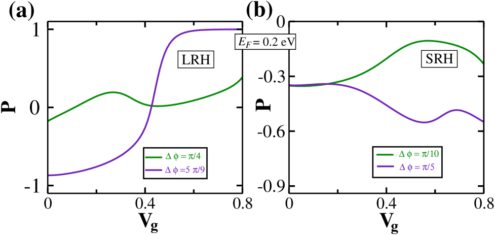
Figure 13: (Color online). Dependence of spin polarization $P$ on $V_{g}$ at two different values of $\Delta\phi$, where (a) $N=19$ and (b) $N=21$. Here we choose $V=0.2\,$V and $\beta=\pi/2$.

further investigate the role of helicity by changing the geometrical conformation associated with the twisting. With the reduction of the twisting angle $\Delta\phi$, the helical shape gradually transforms into the linear-like geometry, and eventually becomes a magnetic chain when $\Delta\phi=0$. This conformational effect should be directly reflected in spin selective electron transmission. This is exactly what we see from Fig. 13, where two typical values of $\Delta\phi$ are taken into account. Both for the LRH and SRH magnetic helices, we find a strong dependence of spin polarization on the twisting angle. For a fixed hopping helix, be it a LRH or SRH one, the degree of polarization sharply decreases with reducing the twisting angle, and the gate voltage $V_{g}$ does not have such an important role under this situation. So, undoubtedly, helicity has an important role in spin polarization.

III.3 Effect of helical dynamics on spin selective transmission

As already noted, for the complete scenario and to have the model more

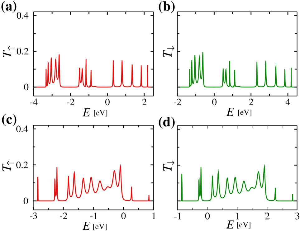
Figure 14: (Color online). Up and down spin transmission probabilities in presence of external gate voltage $V_{g}$, where the top and bottom rows correspond to the LRH and SRH helices, respectively. Here we set $V_{g}=1\,$V, $\beta=0$ and the decay time $\tau=1\,$fs.

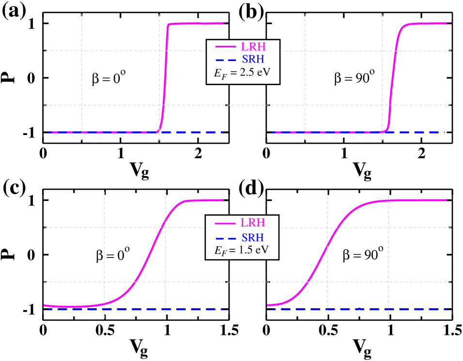
Figure 15: (Color online). $P$-$V_{g}$ characteristics at some typical values of $\beta$ for two different Fermi energies. Here we set $V=0.2\,$V and $\tau=1\,$fs.

realistic we need to include the effect of helical dynamics. In this sub-section we critically examine this issue, where the dynamical effect is included following the prescription given by Ratner and co-workers hd2 .

Let us begin with Fig. 14, where spin dependent transmission probabilities are shown for the LRH helix (upper panel) and the SRH helix (lower panel), considering the decay time $\tau=1\,$fs, keeping all the other parameters unchanged as considered in Fig. 6, to have a better comparison of the spectra obtained for the static (Fig. 6) and dynamic (Fig. 14) cases. At a

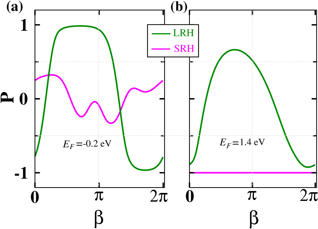
Figure 16: (Color online). Dependence of spin polarization $P$ with phase factor $\beta$ for the two helical geometries. Here we fix $V_{g}=0.5\,$V, $V=0.2\,$V and $\tau=1\,$fs.

first glance we see that the gapped nature of the spectra remains almost identical in the presence of the dynamical effect, like what we notice in the absence of this effect (see Fig. 6). The significant change occurs in transmission amplitudes at the resonances. The amplitude reduces drastically with the helical dynamics. These features can be explained as follows. Due to the addition of a complex part at the acceptor

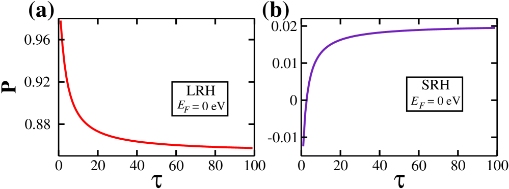
Figure 17: (Color online). Polarization $P$ as a function of decay time $\tau$ (in unit of fs) for the LRH and SRH helices. Here we set $V_{g}=0.5\,$V, $V=0.2\,$V and $\beta=\pi/2$.

site (viz, the site of the MH where the drain electrode is coupled), the effective coupling gets reduced. This coupling significantly influences the electron transfer across the nanojunction, yielding lesser transmission amplitudes.

Though the transmission amplitudes get reasonably hampered due to the dynamical effect, it does not have any considerable influence on spin polarization. It is clearly reflected from the spectra presented in Fig. 15, where the results are computed for $\tau=1\,$fs, setting all the other physical parameters constant as considered in Fig. 8. The underlying physics is that, the spin polarization depends on the ratios of two spin dependent currents. Thus, the reduction of both these two spin currents results almost same degree of spin polarization like what we get in the absence of dynamical effect. It essentially gives a strong confidence that the magnetic helix can be utilized for efficient spin filtration as the spin polarization has not been largely perturbed even in the presence of dynamical effects.

This claim can be justified further by looking into the spectra given in Fig. 16, where the dependence of spin polarization with phase factor $\beta$ is shown, like what are presented earlier in the absence of helical dynamics (see Fig. 9). Almost identical scenario is noticed in both these two cases i.e., in the absence and presence of helical dynamics.

Finally, to have the more comprehensive picture of the effect of helical dynamics, in Fig. 17 we show the dependence of spin polarization on the decay time $\tau$, by varying it in a wide range setting the Fermi energy at zero. Both for the LRH and SRH magnetic helices, we find that the change of $P$ is too small, and remains almost constant for a wide range of $\tau$. This behavior strengthens the robustness of our analysis in the magnetic helix geometry.

IV Summary and Outlook

To conclude, in the present work first time we have addressed the issues of spin selective transmission through a single-stranded magnetic helix, and thoroughly discussed the interplay between the short- and long-range hopping integrals, CISS effect and the role of helical dynamics. We have also explored how to regulate transport properties externally by applying a suitable electric field and changing its orientation, instead of applying a magnetic field as conventionally considered to regulate electron transfer through magnetic materials. All the characteristic features have been studied using the standard Green’s function formalism within the tight-binding framework. The key findings and the important aspects are summarized as follows.
$\bullet$ High degree of spin polarization can be achieved in a magnetic helix, and the performance becomes more superior in the long-range hopping helix rather than the short-range hopping helical geometry.
$\bullet$ A single-stranded MH is capable to yield spin selective transmission, and most importantly, we do not need to include the effects of environmental dephasing.
$\bullet$ The degree of spin polarization along with its phase (positive or negative) can be regulated externally by applying an electric field. Thus, our proposal can be utilized to design externally controlled selective spin transmission.
$\bullet$ The proposed magnetic helix structure exhibits pronounced CISS effect, similar to what is observed in chiral molecules like DNA and others.
$\bullet$ The degree of spin polarization has not been perturbed reasonably even in the presence of helical dynamics. This phenomenon certainly strengthens the robustness of our analysis.
$\bullet$ All the results are valid for a wide range of physical parameters, which prove the robustness of our analysis, and give us a confidence to examine our results in a suitable laboratory setup.
$\bullet$ Our prescription can be implemented in any other magnetic helical geometry having LRH or SRH integrals.

V Acknowledgments

SS is grateful to CSIR, India (File number: 09/093(0183)/2017-EMR-I) for providing her research fellowship. The research of SKM is supported by DST-SERB, India, under Grant number EMR/2017/000504. SKM thanks very much Prof. Shreekantha Sil and Mrs. Moumita Patra for useful discussions. We thank all the reviewers for their valuable comments and suggestions to enhance the quality of the paper.

References

- (1) S. A. Wolf, D. D. Awschalom, R. A. Buhrman, J. M. Daughton, S. von Molnár, M. L. Roukes, A. Y. Chtchelkanova, and D. M. Treger, Science 294, 1488 (2001).
- (2) D. E. Nikonov, G. I. Bourianoff, and P. A. Gargini, J. Supercond. Novel Magn. 19, 497 (2006).
- (3) M. Johnson and R. H. Silsbee, Phys. Rev. Lett. 55, 1790 (1985).
- (4) M. N. Baibich, J. M. Broto, A. Fert, F. Nguyen Van Dau, F. Petroff, P. Etienne, G. Creuzet, A. Friederich, and J. Chazelas, Phys. Rev. Lett. 61, 2472 (1988).
- (5) I. Zutić, J. Fabian, and S. Das Sarma, Rev. Mod. Phys. 76, 323 (2004).
- (6) S. Datta and B. Das, Appl. Phys. Lett. 56, 665 (1990).
- (7) J. P. Lu, J. B. Yau, S. P. Shukla, M. Shayegan, L. Wissinger, U. Rössler, and R. Winkler, Phys. Rev. Lett. 81, 1282 (1998).
- (8) P. Zhang, Q. K. Xue, and X. C. Xie, Phys. Rev. Lett. 91, 196602 (2003).
- (9) W. Long, Q. F. Sun, H. Guo, and J. Wang, Appl. Phys. Lett. 83, 1397 (2003).
- (10) T. P. Pareek, Phys. Rev. Lett. 92, 076601 (2004).
- (11) Q. F. Sun and X. C. Xie, Phys. Rev. B 73, 235301 (2006).
- (12) F. Chi, J. Zheng, and L. L. Sun, Appl. Phys. Lett. 92, 172104 (2008).
- (13) Y. A. Bychkov and E. I. Rashba, Pis’Ma Zh. Eksp. Teor. Fiz. 39, 66 (1984); [JETP Lett. 39, 78 (1984)].
- (14) G. Dresselhaus, Phys. Rev. 100, 580 (1955).
- (15) R. Winkler, Spin-orbit coupling effects in two-dimensional electron and hole Systems, Springer Tracts in Modern Physics, Springer, New York, Vol. 191, (2003).
- (16) J. Nitta, T. Akazaki, H. Takayanagi, and T. Enoki, Phys. Rev. Lett. 78, 1335 (1997).
- (17) J. P. Heida, B. J. van Wees, J. J. Kuipers, T. M. Klapwijk, and G. Borghs, Phys. Rev. B 57, 11911 (1998).
- (18) D. Grundler, Phys. Rev. Lett. 84, 6074 (2000).
- (19) T. Matsuyama, R. Kürsten, C. Meiner, and U. Merkt, Phys. Rev. B 61, 15588 (2000).
- (20) A. A. Kislev and K. W. Kim, J. App. Phys. 94, 4001 (2003).
- (21) I. A. Shelykh, N. G. Galkin, and N. T. Bagraev, Phys. Rev. B 72, 235316 (2005).
- (22) P. Földi, O. Kálmán, M. G. Benedict, and F. M. Peeters, Phys. Rev. B 73, 155325 (2006).
- (23) G. Cohen, O. Hod, and E. Rabani, Phys. Rev. B 76, 235120 (2007).
- (24) S. Ganguly, S. Basu, and S. K. Maiti, Europhys. Lett. 124, 17005 (2018).
- (25) S. Ganguly, S. Basu, and S. K. Maiti, Superlattices Microstruct. 120, 650 (2018).
- (26) W. J. M. Naber, S. Faez, and W. G. van der Wiel, J. Phys. D: Appl. Phys. 40, R205 (2007).
- (27) I. Bergenti, V. Dediu, M. Prezioso, and A. Riminucci, Philos. Trans. R. Soc. London, Ser. A 369, 3054 (2011).
- (28) B. Göhler, V. Hamelbeck, T. Z. Markus, M. Kettner, G. F. Hanne, Z. Vager, R. Naaman, and H. Zacharias, Science 331, 894 (2011).
- (29) Z. Xie, T. Z. Markus, S. R. Cohen, Z. Vager, R. Gutierrez, and R. Naaman, Nano Lett. 11, 4652 (2011).
- (30) R. Naaman and D. H. Waldeck, J. Phys. Chem. Lett. 3, 2178 (2012).
- (31) K. Senthil Kumar, N. Kantor-Uriel, S. P. Mathew, R. Guliamov, and R. Naaman, Phys. Chem. Chem. Phys. 15, 18357 (2013).
- (32) R. Gutiérrez, E. Díaz, R. Naaman, and G. Cuniberti, Phys. Rev. B 85, 081404(R) (2012).
- (33) E. Medina, F. López, M. A. Ratner, and V. Mujica, Europhys. Lett. 99, 17006 (2012).
- (34) A.-M. Guo and Q.-F. Sun, Phys. Rev. Lett. 108, 218102 (2012).
- (35) A.-M. Guo and Q.-F. Sun, Proc. Natl. Acad. Sci. U.S.A. 111, 11658 (2014).
- (36) T.-R. Pan, A.-M. Guo, and Q.-F. Sun, Phys. Rev. B 92, 115418 (2015).
- (37) F. Kuemmeth, S. Ilani, D. C. Ralph, and P. L. McEuen, Nature (London) 452, 448 (2008).
- (38) K.-H. Yoo, D. H. Ha, J.-O. Lee, J. W. Park, J. Kim, J. J. Kim, H.-Y. Lee, T. Kawai, and H. Y. Choi, Phys. Rev. Lett. 87, 198102 (2001).
- (39) G. Maruccio, A. Biasco, P. Visconti, A. Bramanti, P. P. Pompa, F. Calabi, R. Cingolani, R. Rinaldi, S. Corni, R. Di Felice, E. Molinari, M. P. Verbeet, and G. W. Canters, Adv. Mater. 17, 816 (2005).
- (40) K. Bradley, M. Briman, A. Star, and G. Grüner, Nano Lett. 4, 253 (2004).
- (41) A. V. Malyshev, Phys. Rev. Lett. 98, 096801 (2007).
- (42) A.-M. Guo and Q.-F. Sun, Phys. Rev. B 86, 035424 (2012).
- (43) R. Gutiérrez, R. Caetano, P. B. Woiczikowski, T. Kubar, M. Elstner, and G. Cuniberti, New. J. Phys. 12, 023022 (2010).
- (44) F. C. Grozema, Y. A. Berlin, L. D. A. Siebbeles, and M. A. Ratner, J. Phys. Chem. B 114, 14564 (2010).
- (45) F. C. Grozema, S. Tonzani, Y. A. Berlin, G. C. Schatz, L. D. A. Siebbeles, and M. A. Ratner, J. Am. Chem. Soc. 130, 5157 (2008).
- (46) K. Senthilkumar, F. C. Grozema, C. F. Guerra, F. M. Bickelhaupt, F. D. Lewis, Y. A. Berlin, M. A. Ratner, and L. D. A. Siebbeles, J. Am. Chem. Soc. 127, 14894 (2005).
- (47) F. C. Grozema, Y. A. Berlin, and L. D. A. Siebbeles, J. Am. Chem. Soc. 122, 10903 (2000).
- (48) A. Troisi and G. Orlandi, J. Phys. Chem. B 106, 2093 (2002).
- (49) R. N. Barnett, C. L. Cleveland, A. Joy, U. Landman, and G. B. Schuster, Science 294, 567 (2001).
- (50) Y.-H.Su, S.-H. Chen, C. D. Hu, and C.-R. Chang, J. Phys. D: Appl. Phys. 49, 015305 (2016).
- (51) A. A. Shokri, M. Mardaani, and K. Esfarjani, Physica E 27, 325 (2005).
- (52) A. A. Shokri and M. Mardaani, Solid State Commun. 137, 53 (2006).
- (53) M. Dey, S. K. Maiti, and S. N. Karmakar, Phys. Lett. A 374, 1522 (2010).
- (54) M. Patra and S. K. Maiti, Sci. Rep. 7, 14313 (2017).
- (55) A.-M. Guo and Q.-F. Sun, Phys. Rev. B 95, 155411 (2017).
- (56) S. Datta, Electronic Transport in Mesoscopic Systems, Cambridge University Press, Cambridge (1997).
- (57) D. S. Fisher and P. A. Lee, Phys. Rev. B 23, 6851 (1981).
- (58) M. Dey, S. K. Maiti, and S. N. Karmakar, Org. Electron. 12, 1017 (2011).
- (59) D. Rai and M. Galperin, Phys. Rev. B 86, 045420 (2012).
- (60) R. G. Endres, D. L. Cox, and R. R. P. Singh, Rev. Mod. Phys. 76, 195 (2004).
- (61) S. Ganeshan, K. San, and S. Das Sarma, Phys. Rev. Lett. 110, 180403 (2013).
- (62) Y. E. Kraus, Y. Lahini, Z. Ringel, M. Verbin, and O. Zilberberg, Phys. Rev. Lett. 109, 106402 (2012).
- (63) M. Kohmoto, B. Sutherland, and C. Tang, Phys. Rev. B 35, 1020 (1987).
- (64) G. J. Jin, Z. D. Wang, A. Hu, and S. S. Jiang, Phys. Rev. B 55, 9302 (1997).